On the complexity of meander-like diagrams of knots

Abstract.

It is known that each knot has a semimeander diagram (i. e. a diagram composed of two smooth simple arcs), however the number of crossings in such a diagram can only be roughly estimated. In the present paper we provide a new estimate of the complexity of the semimeander diagrams. We prove that for each knot $K$ with more than 10 crossings, there exists a semimeander diagram with no more than $0.31\cdot 1.558^{\operatorname{cr}(K)}$ crossings, where $\operatorname{cr}(K)$ is the crossing number of $K$. As a corollary, we provide new estimates of the complexity of other meander-like types of knot diagrams, such as meander diagrams and potholders. We also describe an efficient algorithm for constructing a semimeander diagram from a given one.

1. Introduction

The diagrams of knots which are composed of two smooth simple arcs (see examples on Fig. 1) were studied under different names by many authors. Apparently, the fact that each knot has such a diagram was first proved by G. Hots in 1960 in [VH60] (for a detailed historical background on this subject see [BM20]). We call such diagrams semimeander diagrams.

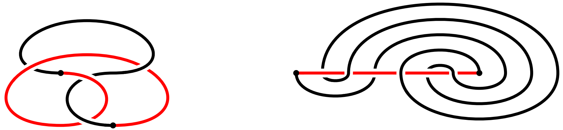
Figure 1. Examples of semimeander diagrams.

In the present paper we study the following question: for a fixed knot $K$ how much a semimeander diagram differs from the minimal diagram of $K$? To be precise, let $K$ be a knot, $\operatorname{cr}(K)$ be its crossing number, and let $\operatorname{cr}_{2}(K)$ be the minimal number of crossings among all semimeander diagrams of $K$. We are interested in finding estimates on $\operatorname{cr}_{2}(K)$ in terms of $\operatorname{cr}(K)$. The first estimates of this kind were given in the works [BM17a] and [Owa18], where it was proved that ${\operatorname{cr}_{2}(K)\leq\sqrt{3}^{\operatorname{cr}(K)}}$. Later, the estimate was improved in [Bel20], where it was claimed that ${\operatorname{cr}_{2}(K)\leq\sqrt[4]{6}^{\operatorname{cr}(K)}}$. However, the proof contained an error, and in fact it was proved that $\operatorname{cr}_{2}(K)\leq\sqrt[4]{8}^{\operatorname{cr}(K)}$. In this paper we improve these estimates and prove the following theorem:

Theorem 1.

Let $K$ be a knot with $\operatorname{cr}(K)>10$, where $\operatorname{cr}(K)$ is the crossing number of $K$, and let $\operatorname{cr}_{2}(K)$ be the minimal number of crossings among all semimeander diagrams of $K$. Then

$$\operatorname{cr}_{2}(K)\leq\frac{208}{431}\sqrt[9]{\frac{8}{431}}\cdot\left(\sqrt[9]{53\frac{7}{8}}\right)^{\operatorname{cr}(K)}\approx 0.31\cdot 1.557^{\operatorname{cr}(K)}.$$

For all knots $K$ with $\operatorname{cr}(K)\leq 10$ the value of $\operatorname{cr}_{2}(K)$ were found explicitly in [Owa18].

Theorem 1 can be used to obtain estimates of the complexity of other classes of meander-like diagrams. For instance, a knot diagram is called meander diagram if it is composed of two smooth simple arcs whose common endpoints lie on the boundary of the convex hull of the diagram (see examples on Fig. 2).

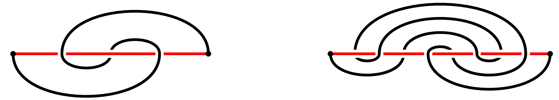
Figure 2. Examples of meander diagrams.

Corollary 1.

Let $K$ be a knot with $\operatorname{cr}(K)>10$, where $\operatorname{cr}(K)$ is the crossing number of $K$, and let $\operatorname{cr}^{mnd}(K)$ be the minimal number of crossings among all meander diagrams of $K$. Then

$$\operatorname{cr}^{mnd}(K)\leq\frac{832}{431}\sqrt[9]{\frac{8}{431}}\cdot\left(\sqrt[9]{53\frac{7}{8}}\right)^{\operatorname{cr}(K)}\approx 1.24\cdot 1.557^{\operatorname{cr}(K)}.$$

Proof.

Let $D$ be a semimeander diagram of $K$ with precisely $\operatorname{cr}_{2}(K)$ crossings. Then there exists a meander diagram of the same knot with at most $4\operatorname{cr}_{2}(K)$ crossings ([BKM⁺22, Lemma 1]). ∎

There is an interesting subclass of meander diagrams, called potholder diagrams, see examples of such diagrams on Fig. 3. The fact that each knot has a potholder diagram was proved in [EZHLN19].

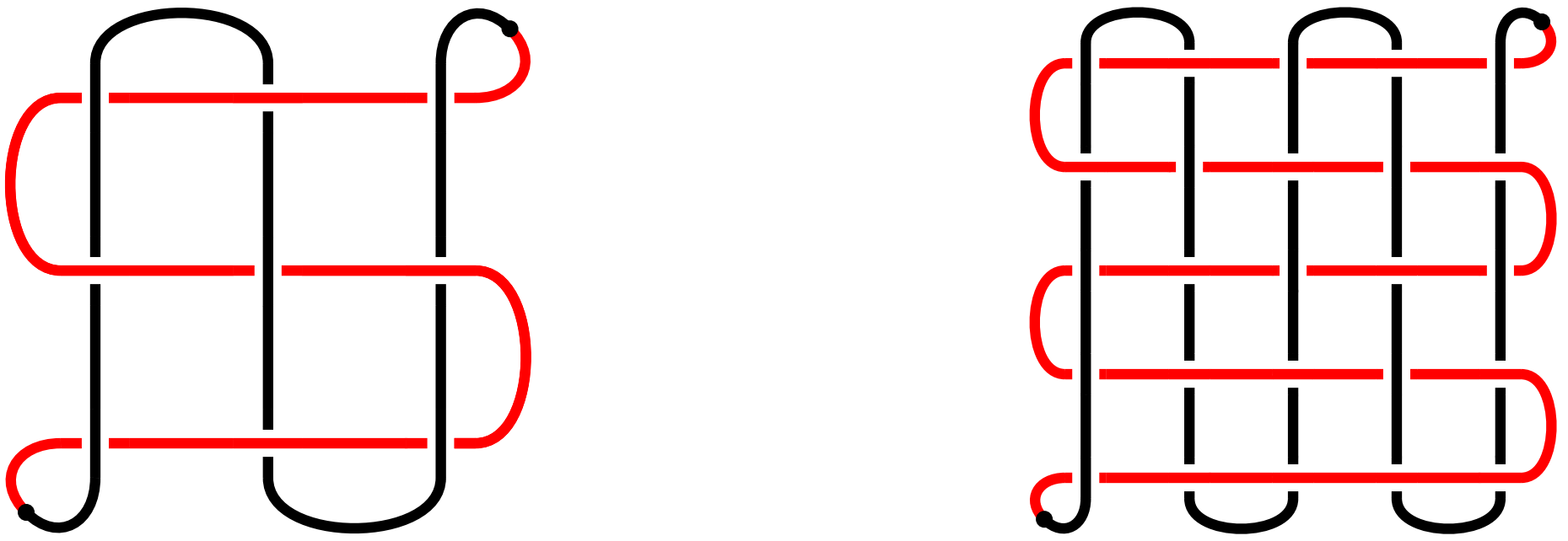
Figure 3. Examples of potholder diagrams.

Corollary 2.

Let $K$ be a knot with $\operatorname{cr}(K)>10$, where $\operatorname{cr}(K)$ is the crossing number of $K$, and let $\operatorname{cr}^{pot}(K)$ be the minimal number of crossings among all potholder diagrams of $K$. Then

$$\operatorname{cr}^{pot}(K)\leq\left(\frac{1664}{431}\sqrt[9]{\frac{8}{431}}\cdot\left(\sqrt[9]{53\frac{7}{8}}\right)^{\operatorname{cr}(K)}-1\right)^{2}\approx\left(2.48\cdot 1.557^{\operatorname{cr}(K)}-1\right)^{2}.$$

Proof.

Let $D$ be a meander diagram of $K$ with precisely $\operatorname{cr}^{mnd}(K)$ crossings. Then there exists a potholder diagram of the same knot with at most $(2\operatorname{cr}^{mnd}(K)-1)^{2}$ crossings ([EZHLN19, Proof of Theorem 1.1]). ∎

In Section 2 the proof of Theorem 1 is presented. The proof is constructive, it involves an analysis of a specific algorithm for constructing a semimeander diagram from a minimal one. In Section 3, a more efficient algorithm for this task is presented.

Acknowledgment

The author expresses gratitude to M. Prasolov for discovering an inaccuracy in author’s work [Bel20], the correction of which led to the proof of the main result of this paper.

2. Proof of Theorem 1

Let $K$ be a knot, let $D$ be its diagram with precisely $n$ crossings, and suppose there is a smooth simple arc $J$ in $D$ such that no endpoint of $J$ is a crossing of $D$. Let $m$ be the number of crossings lying on $J$. We assume $m<n$, otherwise $D$ is already semimeander. The main idea is to successively transform $D$ in such a way that the number of crossings that do not lie on $J$ is reduced (the total number of crossings may increase during these transformations).

Description of transformations

We will consider two types of such transformations: Transformation I ("pulling" the crossing along a simple arc, see Fig. 4) — this is a sequence of so-called $\mathfrak{X}$-moves (see Fig. 5), and Transformation II ("unroll" a simple loop, see Fig. 6). We will consider different sequences of such transformations, and choose the one that increases the total number of crossings the least.

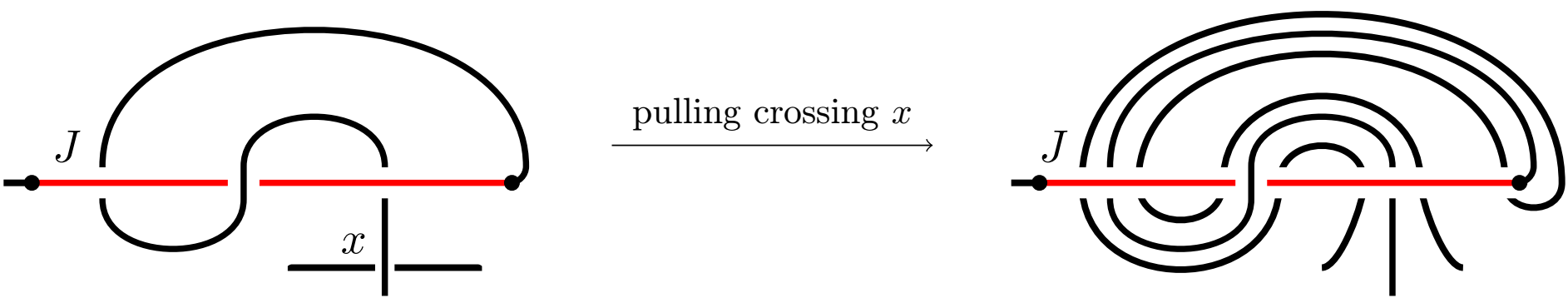
Figure 4. An example of applying Transformation I.

Formally, Transformation I can be described as follows. Let $s_{1}$ and $s_{2}$ be two endpoints of $J$. We can choose an orientation on $D$ in such a way that $J$ is oriented from $s_{1}$ to $s_{2}$. Let’s start moving from $s_{2}$, according to the chosen orientation, to the first crossing $x$ that is not lying on $J$. Since the arc connecting $s_{2}$ and $x$ is simple and contains only crossings that lie on $J$, we can make an $\mathfrak{X}$-move (Fig. 5) with each of them, thus moving $x$ to $J$.

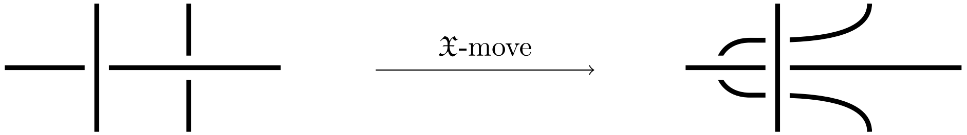
Figure 5. An example of applying $\mathfrak{X}$-move.

Note that if there were precisely $r$ crossings between $x$ and $s_{2}$, the total number of crossings in the diagram will increase by $2r$ after applying Transformation I.

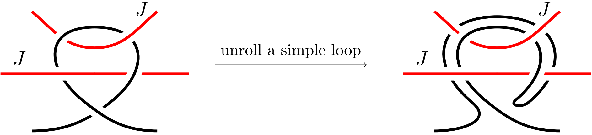
Figure 6. An example of applying Transformation II.

Formally, Transformation II can be described as follows. Let $A$ be a simple loop in $D$ which satisfies the following conditions: (1) the interior of $A$ contains no crossings lying on $D\setminus J$, (2) $J$ is not a subset of $A$, and (3) the crossing $x$ corresponding to the endpoints of $A$ does not lie on $J$. Let $B_{\varepsilon}(A)$ be such a small open neighbourhood of $A$ that the only crossings of $D$ that are contained in $B_{\varepsilon}(A)$ lie on $A$. Now, let $S$ be an arc in $D$ such that (1) $S$ contains the only crossing $x$, (2) $S$ lies in $B_{\varepsilon}(A)$. We can replace $S$ with an arc $S^{\prime}$ with the following properties (1) $S^{\prime}$ has the same endpoints as $S$, (2) $S^{\prime}$ is contained in $B_{\varepsilon}(A)$, and (3) the interior of $S^{\prime}$ does not intersect $D\setminus J$ (over/undercrossings in the new crossings should be set in the obvious way).

Note that if there were precisely $r$ crossings lying on $A$, the total number of crossings in the diagram increases by $r-1$ after applying Transformation II.

Definitions of ACD and preACD

It will be convenient for us to use chord diagrams to study the described Transformations. Let us introduce the necessary technical definitions.

Definition 1.

Let $C$ be a chord diagram with a selected point (we call this point the basepoint). The basepoint and the ends of the chords divide the circle of $C$ into connected components. If each of these connected components and the basepoint are assigned with a positive real number (called weight), then $C$ is called annotated chord diagram, or ACD for short. The length of ACD is the number of chords in it. The complexity of ACD is the weight of the basepoint.

If we label the chords in ACD, we can represent it using Gauss code, additionally placing the weights in square brackets and marking the weight of the basepoint with an over-line (see an example on Fig. 7). The symbols corresponding to the labels of the chords are called non-special.

Definition 2.

A non-cyclic substring of the Gauss code of an ACD is called preACD if it contains the basepoint and the same number of non-special symbols before and after the basepoint. The length of preACD is the number of non-special symbols in it divided by two. The complexity of preACD is the weight of the basepoint.

Let $\mathcal{C}_{k,m}$ be the set of all ACD of length $k$ and of complexity $m$, and let $\mathcal{D}_{k,m}$ be the set of all preACD of length $k$ and of complexity $m$.

To each knot diagram with a selected simple arc one can associate an ACD as follows. Let $D$ be a knot diagram with a selected smooth simple arc $J$ (no endpoint of $J$ are crossings). Let $C$ be a chord diagram corresponding to $D$. Remove from $C$ all chords that have an endpoint on $J$, and contract the arc in $C$ that corresponds to $J$ to a point (this point will be the basepoint in corresponding ACD, and its weight will be equal to the number of crossings lying on $J$). This point and the ends of the remaining chords divide the circle of $C$ into connected components. To each component we assign a number that is equal to the number of chord ends that were removed from that component. See example on Fig. 7. Notice that an ACD $X$ of length zero corresponds to semimeander diagram with number of crossings equals to the complexity of $X$.

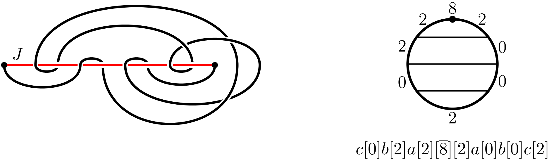
Figure 7. An example of the ACD constructed from a knot diagram.

Transformations I and II in terms of ACD

Transformation I for ACD can be defined as follows. Let $X$ be an ACD of length greater than zero, and let

$$x_{2n}[w_{2n+1}][\overline{m}][w_{1}]x_{1}[w_{2}]x_{2}\dots x_{2n-1}[w_{2n}]$$

be its Gauss code. Transformation I can be performed to eliminate either $x_{1}$ or $x_{2n}$. Let us consider the first case, the second one is similar. Let $x_{1}=x_{i}$ for some $i$ ($2\leq i\leq 2n$). Then after performing Transformation I we obtain an ACD with Gauss code

$$x_{2n}[w_{2n+1}][\overline{m+2w_{1}+1}][w_{1}+w_{2}]x_{2}\dots x_{i-1}[w_{i}+2w_{1}+1+w_{i+1}]x_{i+1}\dots x_{2n-1}[w_{2n}].$$

Transformation II can be described in similar way, but before doing this we need to make two observations.

Observation 1

Let $X$ be an ACD associated to a knot diagram with a selected smooth simple curve, and suppose the Gauss code of $X$ contains a subword of the form

$$\dots x_{1}[w_{1}]x_{2}[w_{2}]x_{2}[w_{3}]x_{1}\dots\ .$$

In this case, Transformation II can be applied twice in such a way that the total number of crossings on a knot diagram does not increase by more than ${w_{1}+2w_{2}+w_{3}-2}$ (see Fig. 8).

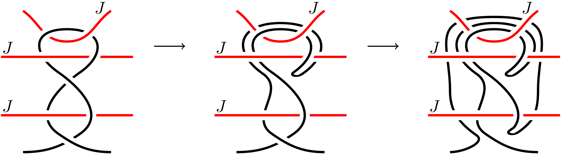
Figure 8. An example of sequential application of Transformation II.

Observation 2

Let $X$ be an ACD associated to a knot diagram with a selected smooth simple curve, and suppose the Gauss code of $X$ contains a subword of the form

$$\dots[\overline{m}][w_{1}]x_{1}[w_{2}]x_{1}[w_{3}]x_{2}\dots\ .$$

In this case, Transformation I can be applied after Transformation II in such a way that the total number of crossings on a knot diagram does not increase by more than $2(w_{1}+2w_{2}+w_{3})-1$ (see Fig. 9).

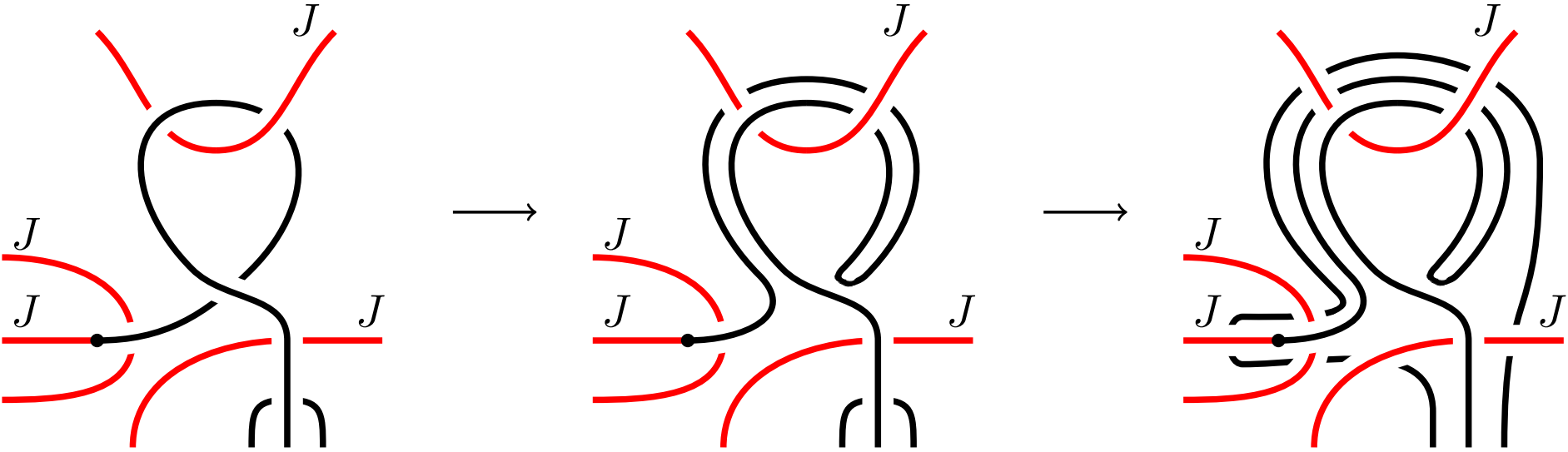
Figure 9. An example of an application of Transformation I after Transformation II.

Based on these two observations, Transformation II for ACD can be defined as follows. Let $X$ be an ACD of length greater than zero, and let

$$x_{2n}[w_{2n+1}][\overline{m}][w_{1}]x_{1}[w_{2}]x_{2}\dots x_{2n-1}[w_{2n}]$$

be its Gauss code. Suppose $x_{i-1}=x_{i}$ for some $i$. After performing Transformation II at $x_{i}$ we obtain an ACD with Gauss code

$$x_{2n}[w_{2n+1}][\overline{m+w_{i}}][w_{1}]x_{1}\dots x_{i-2}[w_{i-1}+w_{i}+w_{i+1}]x_{i+1}\dots x_{2n-1}[w_{2n}].$$

If $X$ is an ACD that was constructed from a knot diagram $D$, each Transformation applied to $X$ corresponds to a analogous Transformation applied to $D$. It is therefore convenient to follow the changes in the number of crossings in the process of constructing a semimeander diagram in terms of ACD. Transformations I and II are transferred verbatim to preACD as well.

Reduce the task to a linear programming problem.

Let $D$ be a diagram of a knot $K$ with a selected smooth simple arc, and let $X\in\mathcal{C}_{k,m}$ be the corresponding ACD with weights $w_{1},w_{2},\dots,w_{2k+1}$. Consider all possible sequences of Transformations I and II eliminating all chords from $X$ (we assume that all of such sequences are numbered from 1 to $r$). A sequence with number $i$ (for $1\leq i\leq r$) gives an ACD of length zero and of complexity $f_{i}(w_{1},\dots,w_{2k+1})$, where

$$f_{i}(w_{1},\dots,w_{2k+1})=\sum_{j=1}^{2k+1}a_{i,j}w_{j}+a_{i,0}$$

is some linear function. Thus starting from $D$ and applying Transformations I and II we can obtain a semimeander diagram of a knot $K$ with no more than $\min\limits_{i=1,\dots,r}f_{i}(w_{1},\dots,w_{2k+1})$ crossings (see example below).

Example 1.

Let $K$ be a knot, let $D$ be its diagram with a selected smooth simple arc on which all but one crossing lie, and let $X$ be the corresponding ACD. $X$ has Gauss code $[\overline{m}][w_{1}]1[w_{2}]1[w_{3}]$ (here we label the only chords with a number 1). There are three possible ways to eliminate the chord (see Fig. 10). So we can obtain a semimeander diagram of $K$ with no more than

$$\min\{m+2w_{1}+1,m+2w_{3}+1,m+w_{2}\}=m+2\frac{m-1}{4}+1=\frac{3m+1}{2}$$

crossings (here we used the fact that $w_{1}+w_{2}+w_{3}=m$).

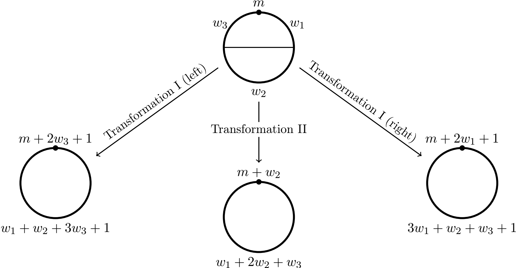
Figure 10. All possible eliminations of a single chord

In general case, if $X$ is an ACD of length $k$ we have the following maximization problem:
Maximize

$$\min_{i=1,2,\dots,r}\left(\sum_{j=1}^{2k+1}a_{i,j}w_{j}+a_{i,0}\right)$$

Subject to

$$\sum_{j=1}^{2k+1}w_{j}\leq m,$$

$$0\leq w_{j}\leq m, 1\leq j\leq 2k+1.$$

This is a standard linear programming problem. Let us rewrite it in the following form:
Maximize

(1) $$t$$

Subject to

(2) $$\sum_{j=1}^{2k+1}w^{\prime}_{j}\leq 1,$$

(3) $$0\leq w^{\prime}_{j}\leq 1, 1\leq j\leq 2k+1,$$

(4) $$t\leq\sum_{j=1}^{2k+1}a_{i,j}w^{\prime}_{j}+\frac{a_{i,0}}{m}, 1\leq i\leq r.$$

Let $\hat{t}(X)$ be the solution of equation (1) for $X$, and let $C_{k,m}=\max\limits_{X\in\mathcal{C}_{k,m}}\hat{t}(X)$. Note that $C_{k,m_{1}}\geq C_{k,m_{2}}$ if $m_{1}\leq m_{2}$, and there exists a limit ${C_{k,\infty}=\lim\limits_{m\to\infty}C_{k,m}}$.

Now let $K$ be a knot with $\operatorname{cr}(K)=n$, and let $D$ be its minimal diagram with a smooth simple arc passing through $m$ crossings. Then there exist a semimeander diagram of $K$ with no more than $mC_{n-m,m}$ crossings. From [BM17b, Theorem 1] it follows that if $\operatorname{cr}(K)>10$ than there exists a minimal diagram of $K$ with a smooth simple arc passing through $m\geq 8$ crossings. Thus for an arbitrary knot $K$ with $n>10$ crossings we get:

$$\operatorname{cr}_{2}(K)\leq 8C_{n-8,8}.$$

The estimation of $C_{k,m}$ using preACD

If $C_{n-8,8}$ is unknown, we can estimate it using preACD. For each preACD $X$ of length $k$, we can consider all possible sequences of Transformation I and II that eliminate $k$ chords, and thus obtain a similar linear problem as (1). Let $X\in\mathcal{D}_{k,m}$, let $\hat{t}(X)$ be a solution of the corresponding linear problem, and let $D_{k,m}=\max\limits_{X\in\mathcal{D}_{k,m}}\hat{t}(X)$.

Now let $K$ be a knot with $\operatorname{cr}(K)=n>10$, let $D$ be its minimal diagram with a smooth simple arc passing through $8$ crossings, and let $d=n-8\ \mathrm{mod}\ k$. Than

$$\operatorname{cr}_{2}(K)\leq 8\left(D_{k,8}\right)^{\left\lfloor\frac{n-8}{k}\right\rfloor}C_{d,8}.$$

$k$	0	1	2	3	4	5	6	7	8	9
$C_{k,8}$	1	$1\frac{9}{16}$	$3\frac{1}{4}$	$4\frac{3}{8}$	$6\frac{2}{5}$	$11\frac{1}{8}$	$14\frac{1}{2}$	$20\frac{1}{8}$	$34\frac{3}{4}$	$44\frac{7}{8}$
$C_{k,\infty}$	1	$1\frac{1}{2}$	3	4	$5\frac{4}{5}$	10	13	18	31	40
$D_{k,8}$	1	$2\frac{1}{8}$	$3\frac{1}{4}$	$4\frac{15}{16}$	$7\frac{3}{4}$	$11\frac{1}{8}$	$16\frac{3}{4}$	$24\frac{5}{8}$	37	$53\frac{7}{8}$
$D_{k,\infty}$	1	2	3	$4\frac{1}{2}$	7	10	15	22	33	48

Table 1. Values of $C_{k,8}$, $C_{k,\infty}$, $D_{k,8}$ and $D_{k,\infty}$ for small $k$.

We found $C_{k,8}$, $C_{k,\infty}$, $D_{k,8}$ and $D_{k,\infty}$ for $k=1,\dots,9$ (see Table 1). The calculation was done with a C++ program that uses the ALGLIB library [Boc] to solve the linear programming problems (the code of the program is available at [Bel]). Thus we get the final estimate:

$$\operatorname{cr}_{2}(K) \leq 8\left(D_{9,8}\right)^{\left\lfloor\frac{\operatorname{cr}(K)-8}{9}\right\rfloor}C_{d,8}\leq\sqrt[9]{D_{9,8}}^{\operatorname{cr}(K)}\frac{8C_{d,8}}{\sqrt[9]{D_{9,8}}^{d+8}}\leq$$

$$\leq\frac{208}{431}\sqrt[9]{\frac{8}{431}}\cdot\left(\sqrt[9]{53\frac{7}{8}}\right)^{\operatorname{cr}(K)}\approx 0.31\cdot 1.557^{\operatorname{cr}(K)}.$$

Remark 1.

$\log(D_{k,8})$, $\log(D_{k,\infty})$, $\log(C_{k,8})$ and $\log(C_{k,\infty})$ grow almost perfectly linearly with increasing $k$ (see Fig. 11). Therefore, we believe that even if values of $C_{k,m}$ will be explicitly determined for all $m$ and $k$, this would not result in an improved estimate beyond $\mathcal{O}\left(1.49^{\operatorname{cr}(K)}\right)$.

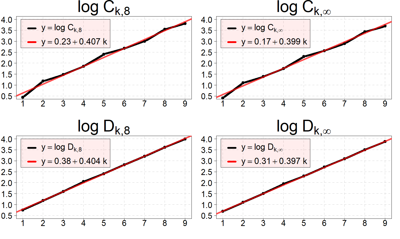
Figure 11. Growth rate of $D_{k,m}$ and $C_{k,m}$.

3. An efficient algorithm for constructing a semimeander diagram

It’s not hard to generalize Transformations I and II. In this section we will explore one approach to achieve this, resulting in an efficient algorithm for constructing a semimeander diagram from a given one.

Let $D$ be a diagram of a knot $K$, and let $J$ be a smooth simple arc in $D$ such that no endpoint of $J$ is a crossing of $D$. For each crossing $x$ in $D$ we can choose two small simple arcs $A_{1}(x)$ and $A_{2}(x)$ with the following properties: (1) both $A_{1}(x)$ and $A_{2}(x)$ contain no crossings other than $x$, (2) their interiors intersect at $x$, (3) $A_{1}(x)$ corresponds to the undercrossing part of $x$. We denote the endpoint of $A_{1}(x)$ by $p_{1}(x)$ and $q_{1}(x)$, and the endpoints of $A_{2}(x)$ by $p_{2}(x)$ and $q_{2}(x)$ (see Fig. 12). A crossing $x$ in $D$ is said to be reducible if there exists a simple curve $\gamma$ with endpoints at $p_{i}(x)$ and $q_{i}(x)$ for some $i\in\{1,2\}$ such that (1) the interior of $\gamma$ intersects $D$ transversally in finite number of double points, and (2) all intersection point between the interior of $\gamma$ and $D$ lie on $J$. Such $\gamma$ is called reduction curve. For each reducible crossing $x$ we define reduction cost to be $\min_{\gamma}|J\cap\gamma|$, where the minimum is taken among all reduction curves $\gamma$.

Figure 12. A neighborhood of a crossing.

Now, for a given diagram $D$ of a knot $K$ we can obtain a semimeander diagram using the following algorithm.

1. Choose a simple arc $J$ in $D$ such that no endpoint of $J$ is a crossing of $D$.

2. If $J$ contains all crossings of $D$ then $D$ is semimeander. Otherwise, we find a reducible crossing $x$ with the smallest reduction cost (denote this reduction cost by $c$).

3. Choose any reduction curve $\gamma$ for $x$ such that the number of intersection points between $\gamma$ and $J$ is equal to $c$.

4. Let the endpoints of $\gamma$ be $p_{i}(x)$ and $q_{i}(x)$ for some $i\in\{1,2\}$. Replace the arc $A_{i}(x)$ with $\gamma$ (over/undercrossings in the new crossings should be set in the obvious way).

5. Repeat steps 2–4 until the diagram becomes a semimeander one.

In practice, this algorithm can be rewritten in terms of the dual graph for a knot diagram. This makes it simple to find reduction costs for all crossings and also to find corresponding reduction curves (for example, using Dijkstra’s algorithm).

References

- [Bel] Yu. Belousov. Semimeander crossing number estimation. https://github.com/YuryBelousov/cr2_estimation.
- [Bel20] Yu. Belousov. Semimeander crossing number of knots and related invariants. Journal of Mathematical Sciences, 251(4):444–452, 2020.
- [BKM+22] Yu. Belousov, M. Karev, A. Malyutin, A. Miller, and E. Fominykh. Lernaean knots and band surgery. St. Petersburg Mathematical Journal, 33(1):23–46, 2022.
- [BM17a] Yu. Belousov and A. Malyutin. Estimates on the semi-meandric crossing number of classical knots. In Polynomial Computer Algebra, pages 21–23, 2017.
- [BM17b] Yu. Belousov and A. Malyutin. Simple arcs in plane curves and knot diagrams. Trudy Instituta Matematiki i Mekhaniki UrO RAN, 23(4):63–76, 2017.
- [BM20] Yu. Belousov and A. Malyutin. Meander diagrams of knots and spatial graphs: Proofs of generalized Jablan–Radović conjectures. Topology and its Applications, 274:107–122, 2020.
- [Boc] S. Bochkanov. ALGLIB. www.alglib.net. Accessed: 2023-11-20.
- [CDM12] S. Chmutov, S. Duzhin, and J. Mostovoy. Introduction to Vassiliev knot invariants. Cambridge University Press, 2012.
- [DFGG97] Ph. Di Francesco, O. Golinelli, and E. Guitter. Meander, folding, and arch statistics. Mathematical and Computer Modelling, 26(8-10):97–147, 1997.
- [EZHLN19] C. Even-Zohar, J. Hass, N. Linial, and T. Nowik. Universal knot diagrams. Journal of Knot Theory and Its Ramifications, 28(07):1950031, 2019.
- [Owa18] N. Owad. Straight knots. arXiv preprint arXiv:1801.10428, 2018.
- [VH60] G. Von Hotz. Arkadenfadendarstellung von knoten und eine neue darstellung der knotengruppe. In Abhandlungen aus dem Mathematischen Seminar der Universität Hamburg, volume 24, pages 132–148. Springer, 1960.