Geometric Thickness of Multigraphs is $\exists\mathbb{R}$-Complete

Abstract

We say that a (multi)graph $G=(V,E)$ has geometric thickness $t$ if there exists a straight-line drawing $\varphi:V\rightarrow\mathbb{R}^{2}$ and a $t$-coloring of its edges where no two edges sharing a point in their relative interior have the same color. The Geometric Thickness problem asks whether a given multigraph has geometric thickness at most $t$. This problem was shown to be NP-hard for $t=2$ [Durocher, Gethner, and Mondal, CG 2016]. In this paper, we settle the computational complexity of Geometric Thickness by showing that it is $\exists\mathbb{R}$-complete already for thickness $57$. Moreover, our reduction shows that the problem is $\exists\mathbb{R}$-complete for $8280$-planar graphs, where a graph is $k$-planar if it admits a topological drawing with at most $k$ crossings per edge. In the course of our paper we answer previous questions on geometric thickness and on other related problems, in particular that simultaneous graph embeddings of $58$ edge-disjoint graphs and pseudo-segment stretchability with chromatic number $57$ are $\exists\mathbb{R}$-complete.

Acknowledgments.

All authors would like to express their gratitude towards the 18th European Research Week on Geometric Graphs which was held in Alcalá de Henares, Spain, in September 2023. The workshop participants, the city, and the university provided a unique experience that made this research possible. T. M. is generously supported by the Netherlands Organisation for Scientific Research (NWO) under project no. VI.Vidi.213.150. I. P. is a Serra Húnter Fellow. S. T. has been funded by the Vienna Science and Technology Fund (WWTF) [10.47379/ICT19035]. We thank Tony Huynh for pointing us at relevant literature about graphs with common edges.

1 Introduction

This paper shows that Geometric Thickness is $\exists\mathbb{R}$-complete, for multi graphs and geometric thickness at least $57$. We start with a tangible example, historic background, and motivation. Then we state our results formally, followed by an in-depth discussion. We round of the introduction by giving an introduction to the existential theory of the reals.

Tangible Examples.

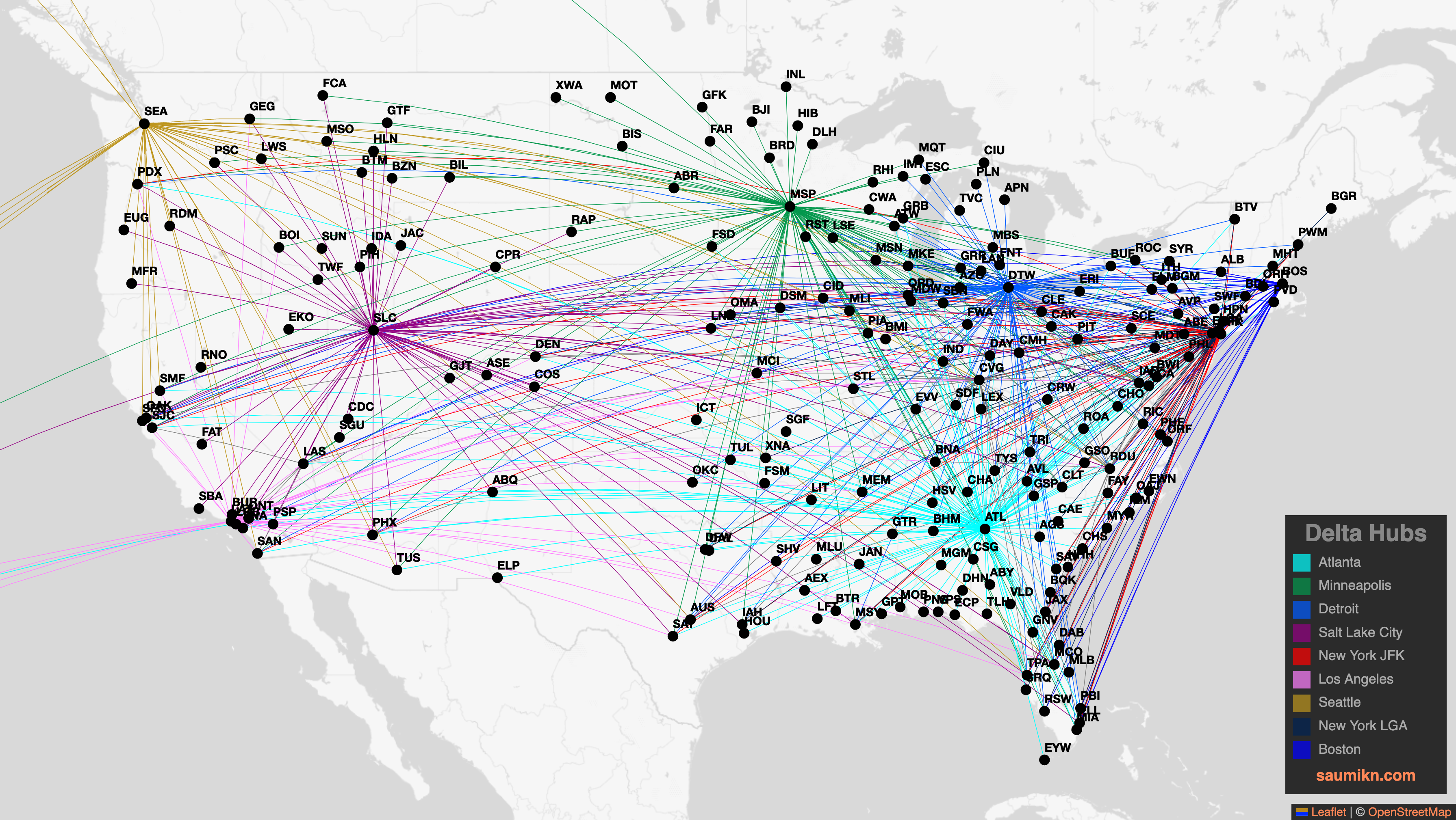
Figure 1: Illustration of Delta airline connections within the continental United States. Connections from different hubs are colored differently. Source: https://saumikn.com/blog/airlinemaps/, used with permission.

Assume you want to visualize the flight network of the continental United States of America, see Figure 1. A natural way to do so is to find a drawing with cities as points and connections by straight lines. Now, if the edges are not crossing this often gives an insightful illustration revealing patterns that are not easily determined by looking at the adjacency matrix. Unfortunately, often networks, like that one, have many edges and it is not possible to attain a planar drawing. In this case, we can color the edges in the drawing. In case that there is no monochromatic crossing and few colors, it is still relatively easy for humans to process the graph in a way that we can extract useful information from it.

In this work, we study the algorithmic question of finding such a drawing together with a correct coloring.

Historic Background.

The thickness of a graph $G$ is the minimum number of planar subgraphs whose union is $G$. It is an old concept; it was formally introduced by Tutte [76] in 1963, but the concept of biplanarity (i.e., geometric thickness 2) had already appeared before, most relevantly, in connection with two open problems: First, Ringel’s Earth–Moon problem on the chromatic number of biplanar graphs [62] and second, a question by Selfridge, formulated by Harary, asking whether $K_{9}$ is biplanar [44, 11, 75]. In 1983, Mansfield [51] showed that deciding whether a graph is biplanar is NP-complete.

In this article we study the geometric or straight-line version of thickness, which requires that all planar subgraphs are embedded simultaneously with straight-line edges. More precisely, a multigraph $G=(V,E)$ has geometric thickness $t$ if there exists a straight-line drawing $\varphi:V\rightarrow\mathbb{R}^{2}$ of $G$ and a $t$-coloring of all the edges such that no two edges of the same color share a point other than a common endpoint. Figure 2 shows an illustration. Note that by definition, two edges connecting the same two endpoints must be assigned distinct colors in the $t$-coloring.

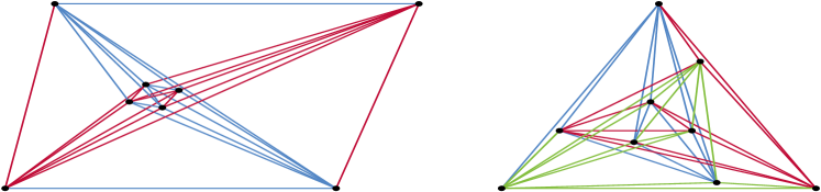
Figure 2: The (geometric) thickness of $K_{8}$ is 2 and of $K_{9}$ is 3.

The concept of geometric thickness was introduced by Dillencourt, Eppstein, and Hirschberg [26], who studied the geometric thickness of complete and complete bipartite graphs. They already asked about the computational complexity of Geometric Thickness, the problem of deciding whether given a graph $G$ and a value $t$, $G$ has geometric thickness at most $t$. Durocher, Gethner, and Mondal [35] partially answered this question by showing that Geometric Thickness is NP-hard even for geometric thickness 2.

Relation Between Geometric Thickness and Other Parameters.

Figure 2 shows straight-line drawings of $K_{8}$ and $K_{9}$ decomposed into two and three plane subgraphs, respectively; these bounds are tight for both the thickness and the geometric thickness. For $n>10$ the thickness of $K_{n}$ is $\lfloor\frac{n+2}{6}\rfloor$ [8, 12] while the geometric thickness, for which no closed formula is known, is lower bounded by $\frac{n}{5.646}$ [26].

In general, the geometric thickness of a graph is not bounded by any function of its thickness. Eppstein [36] proved that for every $t$, there exists a graph with thickness 3 and geometric thickness at least $t$.

The geometric thickness of graphs has also been studied in connection with the degree. The geometric thickness of graphs with maximum degree four is 2 [34]. This result does not generalize: based on counting techniques, Barát, Matoušek and Wood [10] showed that there exist bounded degree graphs with arbitrarily large geometric thickness. A graph is 2-degenerate if every subgraph contains a vertex of degree at most 2. It was recently shown [46] that 2-degenerate graphs have geometric thickness at most 4 and some of them have geometric thickness at least 3.

Regarding the density, Dujmović and Wood [33] showed that every graph with $n\geq 3$ vertices and geometric thickness $k\leq n/2$ has at most $k(3n-k-5)$ edges and there are arbitrarily large graphs with geometric thickness $k$ and $k(3n-4k-3)$ edges.

Motivation.

The Geometric Thickness problem consists of a combination of two computationally hard problems: splitting the edges into color classes and positioning the vertices. The first problem, where we are given the straight-line drawing and the goal is to decompose it into the minimum number of plane subgraphs, corresponds to a graph coloring problem for the corresponding segment intersection graph of the drawing. The 2022 Computational Geometry Challenge focused on this problem [41].

The second problem, when we are given the color classes and the goal is to position the vertices such that no two edges of the same color class intersect in their relative interior, is the Simultaneous Graph Embedding problem, which we will formally define later. Both Simultaneous Graph Embedding and Geometric Thickness connect to applications.

In network visualization, in particular of infrastructure, social, and transportation networks, one often has to deal with intersecting systems of connections belonging to different subnetworks. To represent them simultaneously, different visual variables such as colors are used to indicate edge classes. Drawing the edges with straight-line segments and removing/minimizing same-class crossings is often desirable for readability.

In some settings, the vertex positions can be freely chosen, while the edges classes are given. An example would be visualizing a system of communication channels (phone, email, messenger services) between a set of persons. This case corresponds to the Simultaneous Graph Embedding problem. In other settings, both the positions and the edge classes can be freely chosen, which corresponds to the Geometric Thickness problem. It appears in applications such as VLSI design, where a circuit using uninsulated wires requires crossing wires to be placed on different layers [57].

Since its introduction as a natural measure of approximate planarity [26], geometric thickness keeps receiving attention in Computational Geometry. However, some fundamental questions remain open, including determining the geometric thickness of $K_{n}$ and the complexity of Geometric Thickness. Moreover, the computational methods currently available are not able to provide straight-line drawings of low geometric thickness for graphs with more than a few vertices.

Our results show that, even for small constant values of geometric thickness, computing such drawings is, under widely-believed computational complexity assumptions, harder than any NP-complete problem.

1.1 Results and Related Problems

In this section we state all our results, starting with our main result. To this end, we first need to introduce the complexity class $\exists\mathbb{R}$. The class $\exists\mathbb{R}$ can be defined as the set of problems that are at most as difficult as finding a real root of a multivariate polynomial with integer coefficients. A problem in $\exists\mathbb{R}$ is $\exists\mathbb{R}$-complete if it is as difficult as this problem. We give a more detailed introduction to $\exists\mathbb{R}$ in Section 1.3. We are now ready to state our main result.

Theorem 1.

Geometric Thickness is $\exists\mathbb{R}$-complete for multigraphs already for any fixed thickness $t\geq 57$.

Assuming $\exists\mathbb{R}\neq$ NP, Theorem 1 shows that Geometric Thickness is even more difficult than any problem in NP. This implies that even SAT solvers should not be able to solve Geometric Thickness in full generality. Even more, while a planar graph on $n$ vertices can be drawn on an $n\times n$ grid, there are graphs with geometric thickness $\geq 57$ that will need more than exponentially large integer coordinates for any drawing.

We prove Theorem 1 in Section 2 via a reduction from the problem Pseudo-Segment Stretchability, which we discuss next.

Pseudo-Segment Stretchability.

Schaefer showed that the problem Pseudo-Segment Stretchability (see below for a definition) is $\exists\mathbb{R}$-complete [66]. We closely inspected the proof by Schaefer and observed some small extra properties that we use for our bound in Theorem 1. To state them we first introduce the corresponding definitions.

A pseudo-segment arrangement in $\mathbb{R}^{2}$ is an arrangement of Jordan arcs such that any two arcs intersect at most once. (A Jordan arc is a continuous injective curve from a closed interval to the plane.) A pseudo-segment arrangement $\mathcal{A}$ is called stretchable if there exists a segment arrangement $\mathcal{S}$ such that $\mathcal{A}$ and $\mathcal{S}$ are isomorphic. The curves can be encoded using a planar graph, as it completely determines the isomorphism type which describes the order in which each pseudo-segment intersects all other pseudo-segments. However, in contrast to (bi-infinite) pseudolines, this information is not enough. For example the pseudo-segment arrangement in Figure 3 (left) cannot be stretched, although there exists a segment arrangement with the same intersection pattern (right). Additionally, we require the cyclic order around each intersection point to be maintained.

Figure 3: A stretchable (right) and a non-stretchable (left) pseudo-segment arrangement with the same intersection pattern but different cyclic order around the intersections.

Pseudo-Segment Stretchability asks whether a given pseudo-segment arrangement is stretchable. Schaefer [66] showed that Pseudo-Segment Stretchability is be $\exists\mathbb{R}$-hard, even if each pseudo-segment intersects at most $72$ other pseudo-segments. We consider the intersection graph $G$ of all the pseudo-segments, and we say a pseudo-segment arrangement has chromatic number $\chi$ if and only if the underlying intersection graph $G$ has this chromatic number. We prove the following corollary based on and strengthening a result of Schaefer [66] in Section 5.

Corollary 2 ($\star$$\star$).

Pseudo-Segment Stretchability is $\exists\mathbb{R}$-hard even for pseudo-segment arrangements of chromatic number $57$.

Simultaneous Graph Embedding.

Our main result happens to also resolve a question by Schaefer about simultaneous graph embeddings in the sunflower setting [66]. Before stating the result, we need further definitions. Given simple graphs $G_{1},\ldots,G_{k}$ on the same vertex set $V$, we say $\varphi:V\rightarrow\mathbb{R}^{2}$ is a simultaneous graph embedding, if the straight-line drawing of each $G_{i}$, $i=1,\ldots,k$, on this vertex set is crossing-free. We say $G_{1},\ldots,G_{k}$ form a sunflower if every edge is either in all graphs or in exactly one of the graphs. An edge that is present in all graphs is in the center of the sunflower or a public edge. Edges that are only in one graph are private edges or belonging to a petal of the sunflower. If all edges are private, we say that $G_{1},\ldots,G_{k}$ form an empty sunflower. We define Simultaneous Graph Embedding as the algorithmic problem with $k$ graphs as input that asks if there exists a simultaneous graph embedding.

Corollary 3.

Simultaneous Graph Embedding is $\exists\mathbb{R}$-complete already with $k=58$ and $G_{1},\ldots,G_{k}$ forming an empty sunflower.

The proof can be found in Section 3. In a series of papers it was shown that Simultaneous Graph Embedding is $\exists\mathbb{R}$-complete [23, 39, 65, 66], already for $k=240$. We contribute to this line of research by lowering the bound to $58$ and by restricting it to families of graphs that form an empty sunflower. Lowering the number of graphs from $240$ to $58$ is not so significant as $58$ is still relatively high. The significance lies in the fact that we show $\exists\mathbb{R}$-hardness also for the case that the input graphs form an empty sunflower, which answers a question of Schaefer [66].

Similarly to Geometric Thickness, we would expect that Simultaneous Graph Embedding is $\exists\mathbb{R}$-complete already for two graphs.

Relation Between Geometric Thickness and $k$-Planarity.

In a $k$-planar drawing of a graph each edge can be crossed at most $k$ times. A $k$-planar graph is a graph admitting such a drawing. For the class of $1$-planar graphs, $2$ is a tight upper bound for both the thickness and the geometric thickness. The upper bound for the thickness follows immediately from the degree of the intersection graph. The upper bound of $2$ for the geometric thickness is non-trivial since not every 1-planar graph has a straight-line 1-planar drawing and was only recently shown [18]. This in particular means that the (geometric) thickness of $1$-planar graphs can be decided in polynomial time. In contrast, we show at the end of Section 2 that determining the geometric thickness of $8280$-planar multigraphs is $\exists\mathbb{R}$-complete.

Corollary 4.

Geometric Thickness is $\exists\mathbb{R}$-complete for $8280$-planar multigraphs.

Brandenburg [18] explicitly asked about the geometric thickness of $k$-planar graphs. A combination of previous results [30] shows that simple $k$-planar graphs have bounded geometric thickness: A queue layout of a graph $G$ is a total vertex ordering and a partition of the edges into queues such that no queue contains two nested edges $ad$, $bc$ such that $a<b<c<d$. The queue number $\operatorname{qn}(G)$ of $G$ is the minimum number of queues in such a queue layout. First, geometric thickness is known to be bounded by queue number: any graph $G$ with queue number $\operatorname{qn}(G)$ has geometric thickness $\theta(G)\leq 8\operatorname{qn}(G)^{3}$ [32, Corollary 9]. Second, it was recently shown that any $k$-planar graph $G$ has bounded queue number [29, 31], more precisely $\operatorname{qn}(G)\leq 2\cdot 490^{k+2}$. Together, this yields:

Corollary 5.

Any $k$-planar graph has geometric thickness at most $64\cdot 490^{3(k+2)}$.

Towards Simple Graphs.

Our aim is to resolve the complexity also for simple graphs and in particular for geometric thickness two. For that, it might be desirable to construct a graph in a way that we have some control both about the geometric embedding as well as how the edges are colored. Ideally, we would like to construct a graph in a way that any coloring realizing its geometric thickness leads to the vertices being connected in all colors.

Question 1.

Given $t\in\mathbb{N}$, does there always exist a graph with geometric thickness $t$ such that any $t$-colored drawing of $G$ realizing its geometric thickness is connected in all $t$ colors?

Such a connected construction seems elusive and might not even be possible. It might be worth noting that the minimum number of common edges between any two triangulations is known to be five and eight [45].

Another intriguing question related to our reduction is about the chromatic number of the considered pseudo-segment arrangements, we used in our reduction.

Question 2.

Is Pseudo-Segment Stretchability $\exists\mathbb{R}$-hard even for pseudo-segment arrangements of chromatic number two?

In this direction, we showed that some modifications of Schaefer’s reduction lower the current best bound on the chromatic number for $\exists\mathbb{R}$-hardness from 73 to $57$ in Section 5. However, we believe that considerably new ideas are needed in order to show Question 2. The significance of resolving Question 2 is that it could be a major step to show $\exists\mathbb{R}$-hardness of many graph drawing problems with bounded parameter.

Assuming a positive answer to Question 2, our proof in Section 2 implies directly that Geometric Thickness is $\exists\mathbb{R}$-complete already for geometric thickness two, and Simultaneous Graph Embedding is $\exists\mathbb{R}$-complete for three graphs forming an empty sunflower.

More significantly, we can show the following corollary.

Corollary 6.

Assuming positive answers to Questions 1 and 2, it holds that Geometric Thickness is $\exists\mathbb{R}$-complete already for simple input graphs and thickness 2; see Section 4.

The proof can be found in Section 4. The theorem gives a concrete applications of Questions 2 and 1 and Theorem 1.

1.2 Discussion.

In this section, we discus our results from perspectives not mentioned yet.

Simple Geometric Thickness.

We consider the main weakness of our result that we study multigraphs, instead of simple graphs. Simple graphs are more widely studied in the graph drawing literature and are also arguably more natural as mathematical objects. Furthermore, all previous work consider simple graphs instead of multigraphs. At last, one might also consider that simple graphs may naturally appear in applications, so it would be interesting to know the precise complexity for simple graphs as well. Our motivation to study multigraphs is a precursor to understand simple graphs.

Comparison to Simultaneous Graph Embedding.

Next to Geometric Thickness researchers also studied Simultaneous Graph Embedding. The difference between the two algorithmic problems is that in Geometric Thickness we need to find the embedding and the partition of the edges, whereas in Simultaneous Graph Embedding the partition of the edges is already given. While those problems are formally unrelated, to show $\exists\mathbb{R}$-hardness we need to argue about finding an embedding. This argument gets typically more involved in a reduction for the following reason. An adversary may choose a partition that we did not expect for which it might be much easier to find an embedding. Thus in an $\exists\mathbb{R}$-hardness reduction, we have to argue for correctness for all possible partitions and that is very difficult. On the other hand, as the partition is combinatorial, it is not the part that makes Geometric Thickness $\exists\mathbb{R}$-hard.

Practical Difficulty.

It seems that we know very little about the geometric thickness of even very simple graph classes. For instance, we do not know the geometric thickness of the complete graph $K_{n}$, for all values of $n$ [26]. Given any specific graph or graph class one may always be able to find some arguments tailored to the specific setting. For example, if the max degree is four, we know that the graph has geometric thickness two [34]. We are only aware of two “all purpose” approaches to check the geometric thickness of a graph.

The first one is to encode the problem into an ETR sentence. We know it is possible due to the $\exists\mathbb{R}$-membership, but there is no immediate way how to do this. Furthermore, algorithms to decide an ETR sentence are very slow and might not be feasible for more than 5 or 6 vertices. Note that as $K_{8}$ has geometric thickness two, we can determine the geometric thickness of every graph on up to eight vertices, by checking planarity. Thus, although theoretically possible, this direction seems not very fruitful.

A second approach would be to go through all possible order types of the graph size. Given an order type, we are able with SAT-solvers to decide if the graph can be embedded onto this specific order type using $k$ colors and without monochromatic crossings. This approach could be feasible up to $n=11$, for which there is a database of all order types [7, 59]. Note that feasible does not mean easy, as there are over 2 000 million different order types with 11 points and one would need to check for feasible colorings. In summary, using order types might be feasible but is still very challenging and only possible for graphs of very small order.

1.3 Existential Theory of the Reals

The complexity class $\exists\mathbb{R}$ (pronounced as “ER”) has gained a lot of interest in recent years. It is defined via its canonical complete problem ETR (short for Existential Theory of the Reals) and contains all problems that are polynomial-time many-one reducible to it. In an ETR instance we are given an integer $n$ and a sentence of the form

$$\exists X_{1},\ldots,X_{n}\in\mathbb{R}:\varphi(X_{1},\ldots,X_{n}),$$

where $\varphi$ is a well-formed and quantifier-free formula consisting of polynomial equations and inequalities in the variables and the logical operators $\{\land,\lor,\lnot\}$. The goal is to decide whether this sentence is true. As an example consider the formula $\varphi(X,Y):\equiv X^{2}+Y^{2}\leq 1\land Y^{2}\geq 2X^{2}-1$; among (infinitely many) other solutions, $\varphi(0,0)$ evaluates to true, witnessing that this is a yes-instance of ETR. We find it worth noting that one can define $\exists\mathbb{R}$ with a real witness and a real verification algorithm, similar to the way that NP is defined. The difference is that the witness is allowed to have real number input and the verification runs on the real RAM instead of the word RAM [38]. It is known that

$$\textrm{NP}\subseteq\exists\mathbb{R}\subseteq\textrm{PSPACE}\text{.}$$

Here the first inclusion follows because a SAT instance can trivially be written as an equivalent ETR instance. The second inclusion is highly non-trivial and was first shown by Canny [21].

Note that the complexity of problems involving real numbers was studied in various contexts. To avoid confusion, let us make some remarks on the underlying machine model. As already noted above, the underlying machine model for $\exists\mathbb{R}$ (over which sentences need to be decided and where reductions are performed in) is the word RAM (or equivalently, a Turing machine) and not the real RAM [38] or the Blum-Shub-Smale model [16].

The complexity class $\exists\mathbb{R}$ gains its importance by numerous important algorithmic problems that have been shown to be complete for this class in recent years. The name $\exists\mathbb{R}$ was introduced by Schaefer in [63] who also pointed out that several NP-hardness reductions from the literature actually implied $\exists\mathbb{R}$-hardness. For this reason, several important $\exists\mathbb{R}$-completeness results were obtained before the need for a dedicated complexity class became apparent.

Common features of $\exists\mathbb{R}$-complete problems are their continuous solution space and the nonlinear relations between their variables. Important $\exists\mathbb{R}$-completeness results include the realizability of abstract order types [56, 73] and geometric linkages [64], as well as the recognition of geometric segment [48, 52], unit-disk [53], and ray intersection graphs [22]. More results appeared in the graph drawing community [65, 28, 37, 50], regarding polytopes [4, 6, 27, 60, 61, 78]. Furthermore, other important areas are the study of Nash-equilibria [9, 14, 19, 24, 40, 42, 43, 67], machine learning [3, 13, 17, 54] matrix factorization [49, 68, 70, 71, 72], or continuous constraint satisfaction problems [55]. In computational geometry, we would like to mention the art gallery problem [2, 74], geometric packing [5] and covering polygons with convex polygons [1].

Recently, the community started to pay more attention to higher levels of the “real polynomial hierarchy”, which also capture several interesting algorithmic problems [15, 20, 25, 28, 47, 69].

2 Geometric Thickness is $\exists\mathbb{R}$-Complete

In this section, we first show $\exists\mathbb{R}$-membership. Then we show $\exists\mathbb{R}$-hardness, splitting the proof into construction, completeness, and soundness.

$\exists\mathbb{R}$-membership.

To prove that Geometric Thickness is in $\exists\mathbb{R}$, we follow the characterization provided by Erickson, Hoog, and Miltzow [38]. According to this characterization, a problem $P$ is in $\exists\mathbb{R}$ if and only if there exists a real verification algorithm $A$ for $P$ that runs in polynomial time on the real RAM. Moreover, for every yes-instance $I$ of $P$, there should be a polynomial-size witness $w$ for which $A(I,w)$ returns “yes”. For every no-instance $I$ and any witness $w$, $A(I,w)$ should return “no”.

We now describe a real verification algorithm $A$ for Geometric Thickness. Given an instance $I=(G,t)$, the witness $w$ consists of the coordinates of the vertices of $G$ and a $t$-coloring of the edges $\chi:E\rightarrow{[t]}$.

$A$ then verifies that there are no monochromatic crossings in the induced drawing by examining every pair of edges $e$ and $e^{\prime}$ that cross. Furthermore, $A$ checks that all edges with higher multiplicity receive distinct colors. This verification can be done on a real RAM in $O(|E|^{2})$ time.

Hence, $A$ runs in polynomial time on the real RAM, confirming that Geometric Thickness is in $\exists\mathbb{R}$.

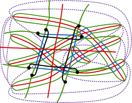
Figure 4: Left: The pseudo-segment arrangement is drawn in red. The tunnel paths are drawn in green. The crossing boxes are drawn in blue and the blockers are not drawn. The connectors are drawn in purple (dotted). Right: Depiction for adding the blockers.

Construction.

We reduce Pseudo-Segment Stretchability to Geometric Thickness. For an illustration of this reduction, we refer to Figure 4. Let $\mathcal{A}$ be a given pseudo-segment arrangement with $n$ pseudo-segments and let $t\geq 57$ be the geometric thickness we are aiming for. We construct a graph $G$ as follows.

• For each pseudo-segment in $\mathcal{A}$, we add one long edge (just a single edge) with multiplicity 1.

• For each crossing, we add a crossing box ($4$-cycle) with multiplicity $t-1$.

• We connect the endpoints of each long edge with the corresponding crossing boxes by tunnel boundaries (paths of length $n$) Tunnel boundaries also connect consecutive crossing boxes.

• We add four blockers (single edges with multiplicity 1) to each crossing box, s.t. they connect corresponding tunnel paths around each crossing box and two blockers cross each pair of opposite crossing box edges.

• We add connectors (paths of length $n$) of multiplicity $t$ between the endpoints of the long edges and the crossing boxes. First, we add a cycle of them between the endpoints of the long edges on the outer face. Then, we “triangulate” the faces that are bounded by tunnel boundaries and connectors by adding connectors such that each such face is incident to three vertices of degree larger than 2. In other words, each such face becomes a triangle after contracting edges incident to degree-2 vertices. Furthermore, we add the paths in such a way that no triangle contains both endpoints of a long segment.

This finishes the construction. Clearly, it can be done in polynomial time. Note that the illustrations of the graph $G$ in Figure 4 are meant to help to understand the definition of $G$. However, we do not know (yet) that the graph $G$ needs to be embedded in the way depicted in the figures.

Completeness.

Let $\mathcal{S}$ be an arrangement of (straight-line segments) such that $\mathcal{S}$ is isomorphic to $\mathcal{A}$. We need to show that there is a drawing of $G$ such that we can color it with $t$ colors avoiding monochromatic crossings.

We start by adding all the edges described in the construction. Note that all added parts are very long, thus, it is easy to see that they offer enough flexibility to realize each edge as a straight-line segment. Next we need to describe a coloring of all edges. The tunnel edges have multiplicity $t$, but they cross no other edges so this is fine. We know that we can color the long edges with $t$ colors due to Corollary 2. Each crossing box edge has multiplicity $t-1$. We use the $t-1$ colors different from the color of the long edge crossing it. Each crossing box has four edges. The two opposite edges receive the same set of colors. The blockers receive the colors of the corresponding long edge that crosses the same crossing box edges. It can be checked that no two edges that cross or overlap have the same color.

Soundness.

We now argue that if $G$ has geometric thickness $t$ then $\mathcal{A}$ is stretchable. Let $\Gamma$ be a straight-line drawing of $G$ with a $t$-coloring of $E$.

Frame.

Let the frame $H$ of $G$ be the subgraph of $G$ that consists only of the crossing boxes, tunnel boundaries, and connectors. Since all edges in $H$ have multiplicity at least $t-1$, no two edges may cross, so $H$ has to be drawn planar. As a first step, we will argue that the frame of $G$ has a unique combinatorial embedding. It is well-known that a planar graph has a unique combinatorial embedding if and only if it is the subdivision of a planar 3-connected graph [58].

Lemma 7.

The frame $H$ of $G$ has a unique combinatorial embedding.

Proof.

First, consider the contracted frame $H^{*}$ obtained as follows; see Figure 5(a). First, contract each tunnel boundary and each connector to a single edge. Then, contract each crossing box to a single vertex and remove multi-edges that appear by the contraction. By construction of the connectors, the resulting graph $H^{*}$ is a planar triangulated graph where each vertex $v^{*}$ corresponds to either the endpoint of a long edge or to a crossing box in $H$, and each edge $e^{*}$ corresponds to either a connector or to two boundary paths in $H$. Since $H^{*}$ is a planar triangulated graph, it has a unique embedding.

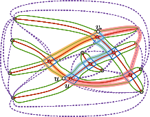
(a) The contracted frame $H^{*}$

(b) Three vertex-disjoint paths in $H$

Figure 5: Illustration for the proof of Lemma 7.

We now argue that $H$ also has a unique embedding by proving that it is the subdivision of a planar 3-connected graph. Obviously, $H$ has no vertices of degree 1. Hence, we only have to prove that there are three vertex-disjoint simple paths between any two vertices of degree at least 3. Let $u,v$ be two such vertices of $H$.

First, assume that $u$ and $v$ belong to the same crossing box. If $u$ and $v$ are adjacent, then they share two common faces. One of the two faces is the interior of the crossing box, the other face is bounded by two tunnel boundaries and the endpoint of a long edge or an edge of a different crossing box. We obtain the three paths from the edge $(u,v)$ and from following the boundaries of the common faces. If $u$ and $v$ are not adjacent, we find two paths following the edges of the crossing box. For the third path, let $w^{*}$ be the corresponding vertex in $H^{*}$, let $e_{u}$ and $e_{v}$ be tunnel paths incident to $u$ and $v$, respectively, and let $e^{*}_{u}$ and $e^{*}_{v}$ be the edges of $H^{*}$ that correspond to $e_{u}$ and $e_{v}$, respectively. Since $H^{*}$ is 3-connected, there exists a cycle $C^{*}=\langle w^{*},e^{*}_{0},w_{1}^{*},e_{1}^{*},\ldots,e_{k-1}^{*},w_{k}^{*},e_{k}^{*},w^{*}\rangle$ in $H^{*}$ through $e_{u}^{*}=e_{0}^{*}$ and $e_{v}^{*}=e_{k}^{*}$. We find a path $P$ from $u$ to $v$ in $H$ by replacing each edge $e_{i}^{*}$ of $C^{*}$ by the corresponding tunnel path or connector in $H$, and each vertex $w_{k}^{*}$ by the corresponding vertex or a path through the corresponding crossing box.

Now, assume that $u$ and $v$ do not belong to the same crossing box. Let $u^{*}$ and $v^{*}$ be the vertices of $H^{*}$ corresponding to $u$ and $v$, respectively. Let $P_{1}^{*},P_{2}^{*},P_{3}^{*}$ be three vertex-disjoint paths between $u^{*}$ and $v^{*}$ in $H^{*}$. Similar to the previous case, we aim to find three paths $P_{1},P_{2},P_{3}$ by replacing the edges of $P_{1}^{*},P_{2}^{*},P_{3}^{*}$ by corresponding tunnel paths or connectors and interior vertices by paths through corresponding crossing boxes, if necessary. Since the paths are vertex-disjoint, we do not visit any crossing boxes more than once, except those of $u$ and $v$. In fact, if $u$ is a vertex of a crossing box, it might happen that the tunnel paths that correspond to the first edges of $P_{1},P_{2},P_{3}$ do not start in $u$, but in different vertices of the crossing box of $u$.

To get rid of this problem, we now prove a slightly stronger version of Menger’s theorem. (We believe that this statement might have been proven before. We include a proof here for completeness.) Let $G$ be a 3-connected graph with vertices $u$ and $v$ and edges $e_{u}=(u,u^{\prime})$ and $e_{v}=(v,v^{\prime})$. Then there exist three interior-vertex-disjoint paths $P_{1},P_{2},P_{3}$ from $u$ to $v$ such that $e_{u},e_{v}\in P_{1}\cup P_{2}\cup P_{3}$. First, find three interior-vertex-disjoint paths $P_{1}^{\prime},P_{2}^{\prime},P_{3}^{\prime}$ from $u$ to $v$. If these paths contain $e_{u}$ and $e_{v}$, we are done. Otherwise, assume that they do not contain $e_{u}$. By 3-connectivity, there are three vertex-disjoint paths from $u^{\prime}$ to $v$, so at least one of them does not visit $u$. Let $Q$ be this path. If $Q$ is interior-vertex-disjoint from two of $P^{\prime}_{1},P^{\prime}_{2},P^{\prime}_{3}$, say $P^{\prime}_{2}$ and $P^{\prime}_{3}$, then $P_{1}=\langle u,e_{u},Q\rangle,P^{\prime}_{2},P^{\prime}_{3}$ are three interior-vertex-disjoint paths from $u$ to $v$ with $e_{u}\in P_{1}$. Otherwise, follow $Q$ until it reaches an interior vertex of $P^{\prime}_{1},P^{\prime}_{2},P^{\prime}_{3}$ for the first time, say vertex $w$ on $P^{\prime}_{1}$. Create a path $P_{1}$ from $u$ to $v$ by following $e_{u}$, then $Q$ until reaching $w$, then $P^{\prime}_{1}$ until reaching $v$. Then $P_{1},P^{\prime}_{2},P^{\prime}_{3}$ are three interior-vertex-disjoint paths from $u$ to $v$ with $e_{u}\in P_{1}$. We can force $e_{v}$ to be part of one of the paths analogously.

Hence, we can assume that at least one of $P_{1},P_{2},P_{3}$ starts with a tunnel path at $u$ and at least one of $P_{1},P_{2},P_{3}$ ends with a tunnel path at $v$. For the other two paths at $u$, we can reach the endpoint of the first tunnel path by following the crossing box, if necessary. An analogous argument works for that last edges to reach $v$. ∎

As a next step, we will define tunnels precisely.

Tunnels.

In Figure 6, we illustrate the regions in the plane that we refer to as middle tunnel segments, end tunnel segments, and crossing boxes. We believe that those notions are very easy to understand for the reader from the figure and thus we avoid a formal definition. (End or middle) tunnel segments incident to the same crossing box are called consecutive.

Figure 6: Each tunnel consists of two end tunnel segments and various middle tunnel segments, separated by crossing boxes.

We say that a tunnel segment has color $c$, if it contains a long segment with color $c$. We will show that each tunnel segment has exactly one color.

Claim 1.

Each end tunnel segment contains at least one long segment.

Consider any long edge $\ell$ and the frame $H^{\prime}$ without the blockers, and any embedding of $H^{\prime}\cup\{\ell\}$. Since the frame has a unique combinatorial embedding and a long edge cannot cross a tunnel boundary or connector (as they have multiplicity $t$), this embedding must be plane and coincide with the unique combinatorial embedding of $H$ on $H^{\prime}$. The only way to add $\ell$ into the embedding of $H^{\prime}$ is through its end tunnel segment.

Claim 2.

Each tunnel segment has at most one color $c$ and its bounding crossing box edges have all the remaining colors.

Note that each tunnel segment can only be entered or left by a long segment using the multiedges of the crossing box. As those have multiplicity $t-1$, it follows that the edges of the crossing box are colored with all colors except the color of the long segment. Now, we see that each tunnel segment is completely surrounded by edges of all but one colors, which implies the claim.

Figure 7: Consecutive tunnel segments must have the same color.

Claim 3.

Consecutive tunnel segments have the same color.

See Figure 7, for an illustration. Denote by $S,T$ the two consecutive tunnel segments and by $C=[t]$ the set of all colors. Say tunnel $S$ has color $c$. We show that tunnel $T$ has the same color. Due to the unique embedding there is a blocker that intersects both tunnels. As the blocker is in a tunnel with color $c$, the bounding crossing box edges have colors $C\setminus c$. Thus, the blocker must have color $c$ as well. Hence, also $T$ must have color $c$ as all bounding crossing box edges must have colors $C\setminus c$ (unless they are uncrossed). This proves the claim and also immediately the following:

Claim 4.

All tunnel segments of a tunnel have the same color.

We are now ready to show our central claim:

Claim 5.

Each long segment stays in its respective tunnel.

First, we note that all the blockers of a tunnel have the same color as the long edge. Furthermore, due to the combinatorial embedding, the tunnel paths together with the blockers form a cycle surrounding the long segment. It remains to show that the blockers cannot leave the tunnel, to show that the long segments cannot leave the tunnel. To this end, notice that a blocker cannot cross a crossing box edge twice, because they are both line segments and two line segments can cross at most once.

Claim 6.

The arrangement $\mathcal{S}$ formed by the long segments is combinatorially equivalent to the arrangement $\mathcal{A}$ of pseudo-segments.

This follows from the tunnels crossing combinatorially as in arrangement $\mathcal{A}$ and the long segments staying within their respective tunnels.

Claim 6 concludes the proof of Theorem 1. Notice that in our construction, for every crossing, we add $2t$ more crossings ($2(t-1)$ from the parallel crossing box edges and two from the blockers). Since the pseudo-segment graph from Schaefer’s construction has maximum degree 72 [63], the graph in our reduction is $8280$-planar, which proves Corollary 4.

3 Sunflower Simultaneous Graph Embedding

This section is devoted to proving Corollary 3 by slightly modifying our construction in the proof of Theorem 1. We reduce Pseudo-Segment Stretchability to Simultaneous Graph Embedding with the additional restriction that the input graphs of the Simultaneous Graph Embedding instance form an empty sunflower. To this end, let $\mathcal{A}$ denote a pseudo-segment arrangement with $n$ pseudo-segments. Further, let $c$ be the chromatic number of the pseudo-segment intersection graph induced by $\mathcal{A}$ and let $\chi:\mathcal{A}\rightarrow[c]$ denote a corresponding $c$-coloring.

We construct an instance of Simultaneous Graph Embedding consisting of $k:=c+1$ simple graphs $H,G_{1},\ldots,G_{c}$ on a shared vertex set as follows. The graph $H$ contains exactly the edges belonging to the frame graph as defined above, i.e., the crossing boxes, the tunnel boundaries and the connectors. Moreover, for $i\in[c]$, the graph $G_{i}$ contains the long edges corresponding to each pseudo-segment $S\in\mathcal{A}$ for which $\chi(S)=i$ and a $1$-subdivision of the edges of $H$ aside from the crossing box edges bounding tunnel segments corresponding to pseudo-segments $S\in\mathcal{A}$ for which $\chi(S)=i$. More precisely, in the $1$-subdivision of the subgraph of $H$ belonging to $G_{i}$, each edge $e=(u,v)$ of $H$ is replaced by a path $(u,x_{i}(e),v)$ of length $2$ where $x_{i}(e)$ does not belong to $H$, i.e., $x_{i}(e)$ is an isolated vertex in all graphs except for $G_{i}$. Since $\chi$ is a proper $c$-coloring, the graphs $G_{1},\ldots,G_{c}$ do not share any long edges, while their $1$-subdivisions of $H$ are edge-disjoint by construction. As also $H$ is edge-disjoint from any of the $1$-subdivisions, we observe that $H,G_{1},\ldots,G_{c}$ form an empty sunflower. Note that the construction here does not require any blockers.

It remains to discuss that $\mathcal{A}$ is stretchable if and only if $H,G_{1},\ldots,G_{c}$ admit a simultaneous geometric embedding. First, completeness can be easily shown following the argumentation in the corresponding paragraph in Section 2. In particular, we need to discuss how to place the subdivision vertices of edges of $H$. Namely, for an edge $e=(u,v)$ of $H$, we can place all subdivision vertices $x_{i}(e)$ arbitrarily close to the straight-line segment representing $(u,v)$. Completeness now immediately follows by observing that $G_{i}$ contains no subdivisions of crossing-box edges that bound tunnel segments corresponding to a pseudo-segment $S\in\mathcal{A}$ for which $\chi(S)=i$, i.e., the tunnel of a segment $S\in\mathcal{A}$ with $\chi(S)=i$ is a single face in $G_{i}$ minus the long edge representing $S$.

Figure 8: In our construction for proving Corollary 3, subdivided tunnels do not contain subdivisions of crossing box edges shared by consecutive segments. While subdivided tunnels may cover not all of the tunnel and also additional parts of the plane, each curve connecting between both end segments traverses all segments in order.

Finally, we show soundness. Let $\varphi$ be a simultaneous geometric embedding of $H,G_{1},\ldots,G_{c}$. For a pseudo-segment $S\in\mathcal{A}$, we define the subdivided tunnel as the $1$-subdivision of the outer cycle of its tunnel belonging to $G_{\chi(S)}$; see Figure 8. Note that $G_{\chi(S)}$ does not contain a subdivision of the crossing box edges shared by consecutive segments of a subdivided tunnel; see dotted edges in Figure 8. We now prove the equivalent of Claim 5:

Claim 7.

Each long segment traverses all segments and crossing boxes of its respective tunnel in order.

First note that by Lemma 7, we know that $H$ has a unique combinatorial embedding. Now consider a pseudo-segment $S$ with $\chi(S)=i$. Since $G_{i}$ contains subdivisions of all tunnel boundaries and all connectors, the corresponding long edge $\ell$ must be drawn completely inside tunnels. By construction, the endpoints of $\ell$ are contained only on the boundary of the subdivided tunnel corresponding to $S$, i.e., it must start and end inside its respective subdivided tunnel. Moreover, by construction, the entire subdivided tunnel belongs to $G_{i}$. Thus, $\ell$ cannot enter other tunnels in between. While the subdivided tunnel may be covering a superset of the tunnel, $\ell$ must still traverse all of its segments as the crossing box edges between consecutive segments still separate subdivided segments.

The fact that each long edge still traverses each crossing box in order implies immediately Claim 6 in our reduction to Simultaneous Graph Embedding and the theorem follows.

4 Towards Simple Geometric Thickness

This section is devoted to showing the following implication to a positive answer to Questions 1 and 2.

Theorem 8.

Assuming positive answers to Questions 1 and 2, it holds that Geometric Thickness is $\exists\mathbb{R}$-complete already for simple input graphs and thickness 2.

Proof.

The proof goes by some small modifications of the proof of Theorem 1. In order to avoid reiterating all the arguments again, which are almost identical to the previous proof, we only highlight the modifications. We first observe that a positive answer to Question 2 implies that we can reduce from 2-colorable Pseudo-Segment Stretchability. Thus, we would only need edges of multiplicity 2 in the reduction. Edges of multiplicity $t-1$ are now just normal edges and we do not need to worry about them. Furthermore, our geometric thickness parameter would also drop to 2 by just following the reduction and replacing $57$ by 2 everywhere.

As a next step, we use the answer to Question 1 for the case of geometric thickness 2. That is, we may assume that there is a graph $F$ of geometric thickness equal to 2 that is connected in every color in any possible realization. We replace every edge of multiplicity 2 by a copy of $F$, with two vertices of $F$ being identified with the endpoints that $F$ replaces.

This step takes constant time per edge, as $F$ is a fixed graph. Furthermore, if the graph had geometric thickness 2 before, it has still geometric thickness 2 after the modification. To see this, take a drawing of the original multiedge $e$ and replace it by a very thin drawing of $F$ using two colors. Furthermore, the arguments about the edges with higher multiplicity never used straightness of the edges, only topological connectedness. Those arguments equally apply to $F$ instead of the original edge $e$. This finishes the proof. ∎

5 Chromatic Number of Pseudo-Segment Arrangements

In this section, we will show that the pseudo-segment arrangement from Schaefer’s construction has chromatic number $\leq 57$.

See 2

Proof.

The pseudo-segment graph $G$ from Schaefer’s construction has maximum degree 72, so it trivially has chromatic number at most 73. We will observe that the chromatic number is significantly lower.

Schaefer first constructs a pseudo-segment arrangement that is not uniform, i.e., it can happen that three or more segments cross in a single point. The underlying intersection graph $G^{\prime}$ has maximum degree 18, so it has chromatic number at most 19. However, the machinery only works with uniform pseudo-segment arrangements, so he shows that his construction yields a so-called constructible arrangement and uses the dual of a technique by Las Vergnas [77] to make the arrangement uniform. To this end, some pseudo-segments are replaced by 2 or 4 other pseudo-segments as shown in Figure 9, which increases the number of crossings per segments (and thus the maximum degree of $G^{\prime}$) by a factor 4 to 72. However, it is straight-forward to see that these replacements increase the chromatic number by at most factor 3 to $57$:

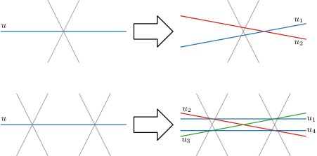
Figure 9: Making a pseudo-segment arrangement uniform while increasing the chromatic number by factor 3.

Let $\chi^{\prime}$ be a 19-coloring of $G^{\prime}$ where every vertex $u$ has a color $c^{\prime}(u)\in\{c_{1},\ldots,c_{19}\}$. We obtain a $57$-coloring $\chi$ of $G$ where every vertex $v$ has a color $c(v)\in\{c_{1}^{1},c_{1}^{2},c_{1}^{3},\ldots,c_{19}^{1},c_{19}^{2},c_{19}^{3}\}$ as follows. Let $u$ be a vertex in $G^{\prime}$ with color $c^{\prime}(u)=c_{i}$. If $u$ is not replaced in the construction, we set $c(u)=c_{i}^{1}$. If $u$ is replaced by two vertices $u_{1},u_{2}$, we set $c(u_{1})=c_{i}^{1}$ and $c(u_{2})=c_{i}^{2}$. If $u$ is replaced by four vertices $u_{1},u_{2},u_{3},u_{4}$, observe that $u_{1}$ and $u_{2}$ are not adjacent; see Figure 9(bottom). Hence, we can set $c(u_{1})=c(u_{4})=c_{i}^{1}$, $c(u_{2})=c_{i}^{2}$, and $c(u_{3})=c_{i}^{3}$. ∎

References

- [1] Mikkel Abrahamsen. Covering polygons is even harder. In 2021 IEEE 62nd Annual Symposium on Foundations of Computer Science—FOCS 2021, pages 375–386. IEEE Computer Soc., 2022. doi:10.1109/FOCS52979.2021.00045.
- [2] Mikkel Abrahamsen, Anna Adamaszek, and Tillmann Miltzow. The art gallery problem is -complete. In STOC’18—Proceedings of the 50th Annual ACM SIGACT Symposium on Theory of Computing, pages 65–73. ACM, New York, 2018. doi:10.1145/3188745.3188868.
- [3] Mikkel Abrahamsen, Linda Kleist, and Tillmann Miltzow. Training neural networks is ER-complete. In Advances in Neural Information Processing Systems 34: Annual Conference on Neural Information Processing Systems 2021, NeurIPS 2021, pages 18293–18306, 2021. URL: https://proceedings.neurips.cc/paper/2021/hash/9813b270ed0288e7c0388f0fd4ec68f5-Abstract.html.
- [4] Mikkel Abrahamsen, Linda Kleist, and Tillmann Miltzow. Geometric embeddability of complexes is -complete. In 39th International Symposium on Computational Geometry, volume 258 of LIPIcs, pages Art. No. 1, 19. Schloss Dagstuhl. Leibniz-Zent. Inform., Wadern, 2023. doi:10.4230/lipics.socg.2023.1.
- [5] Mikkel Abrahamsen, Tillmann Miltzow, and Nadja Seiferth. Framework for ER-completeness of two-dimensional packing problems. In 2020 IEEE 61st Annual Symposium on Foundations of Computer Science, pages 1014–1021. IEEE Computer Soc., 2020. doi:10.1109/FOCS46700.2020.00098.
- [6] Karim A. Adiprasito, Arnau Padrol, and Louis Theran. Universality theorems for inscribed polytopes and Delaunay triangulations. Discrete Comput. Geom., 54(2):412–431, 2015. doi:10.1007/s00454-015-9714-x.
- [7] Oswin Aichholzer, Franz Aurenhammer, and Hannes Krasser. Enumerating order types for small point sets with applications. Order, 19(3):265–281, 2002. doi:10.1023/A:1021231927255.
- [8] V. B. Alekseev and V. S. Gončakov. The thickness of an arbitrary complete graph. Mathematics of the USSR-Sbornik, 30(2):187, 1976. doi:10.1070/SM1976v030n02ABEH002267.
- [9] Luc Attia and Miquel Oliu-Barton. Stationary equilibria in discounted stochastic games. Dynamic Games and Applications, pages 1–14, 2023. doi:10.1007/s13235-023-00495-x.
- [10] János Barát, Jirí Matousek, and David R. Wood. Bounded-degree graphs have arbitrarily large geometric thickness. Electron. J. Comb., 13(1), 2006. doi:10.37236/1029.
- [11] Joseph Battle, Frank Harary, and Yukihiro Kodama. Every planar graph with nine vertices has a nonplanar complement. Bull. Am. Math. Soc., 68:569–571, 1962. doi:10.1090/S0002-9904-1962-10850-7.
- [12] Lowell W. Beineke and Frank Harary. The thickness of the complete graph. Canadian J. Math., 17:850–859, 1965. doi:10.4153/CJM-1965-084-2.
- [13] Daniel Bertschinger, Christoph Hertrich, Paul Jungeblut, Tillmann Miltzow, and Simon Weber. Training fully connected neural networks is -complete. CoRR, abs/2204.01368, 2022. arXiv:2204.01368, doi:10.48550/arXiv.2204.01368.
- [14] Vittorio Bilò, Kristoffer Arnsfelt Hansen, and Marios Mavronicolas. Computational complexity of decision problems about nash equilibria in win-lose multi-player games. In Argyrios Deligkas and Aris Filos-Ratsikas, editors, Algorithmic Game Theory, pages 40–57, Cham, 2023. Springer Nature Switzerland. doi:10.1007/978-3-031-43254-5\_3.
- [15] Manon Blanc and Kristoffer Arnsfelt Hansen. Computational complexity of multi-player evolutionarily stable strategies. In Computer science—theory and applications, volume 12730 of Lecture Notes in Comput. Sci., pages 1–17. Springer, Cham, 2021. doi:10.1007/978-3-030-79416-3\_1.
- [16] Lenore Blum, Mike Shub, and Steve Smale. On a theory of computation and complexity over the real numbers: NP-completeness, recursive functions and universal machines. Bulletin of the American Mathematical Society, 21(1):1–46, 1989. doi:10.1090/S0273-0979-1989-15750-9.
- [17] Tobias Boege. The Gaussian conditional independence inference problem. PhD thesis, Universität Magdeburg, 2022.
- [18] Franz J. Brandenburg. Straight-line drawings of 1-planar graphs. CoRR, abs/2109.01692, 2021. URL: https://arxiv.org/abs/2109.01692, arXiv:2109.01692.
- [19] Romain Brenguier. Robust equilibria in mean-payoff games. In Foundations of software science and computation structures, volume 9634 of Lecture Notes in Comput. Sci., pages 217–233. Springer, Berlin, 2016. doi:10.1007/978-3-662-49630-5\_13.
- [20] Peter Bürgisser and Felipe Cucker. Exotic quantifiers, complexity classes, and complete problems. Found. Comput. Math., 9(2):135–170, 2009. doi:10.1007/s10208-007-9006-9.
- [21] John Canny. Some Algebraic and Geometric Computations in PSPACE. In Proceedings of the Twentieth Annual ACM Symposium on Theory of Computing (STOC ’88), pages 460–467, 1988. doi:10.1145/62212.62257.
- [22] Jean Cardinal, Stefan Felsner, Tillmann Miltzow, Casey Tompkins, and Birgit Vogtenhuber. Intersection graphs of rays and grounded segments. J. Graph Algorithms Appl., 22(2):273–295, 2018. doi:10.7155/jgaa.00470.
- [23] Jean Cardinal and Vincent Kusters. The complexity of simultaneous geometric graph embedding. J. Graph Algorithms Appl., 19(1):259–272, 2015. doi:10.7155/jgaa.00356.
- [24] Krishnendu Chatterjee and Rasmus Ibsen-Jensen. The complexity of ergodic mean-payoff games. In Automata, languages, and programming. Part II, volume 8573 of Lecture Notes in Comput. Sci., pages 122–133. Springer, Heidelberg, 2014. doi:10.1007/978-3-662-43951-7\_11.
- [25] Julian D’Costa, Engel Lefaucheux, Eike Neumann, Joël Ouaknine, and James Worrell. On the complexity of the escape problem for linear dynamical systems over compact semialgebraic sets. In 46th International Symposium on Mathematical Foundations of Computer Science, volume 202 of LIPIcs, pages Art. No. 33, 21. Schloss Dagstuhl. Leibniz-Zent. Inform., Wadern, 2021. doi:10.4230/LIPIcs.MFCS.2021.33.
- [26] Michael B. Dillencourt, David Eppstein, and Daniel S. Hirschberg. Geometric thickness of complete graphs. J. Graph Algorithms Appl., 4(3):5–17, 2000. doi:10.7155/jgaa.00023.
- [27] Michael Gene Dobbins, Andreas F. Holmsen, and Tillmann Miltzow. A universality theorem for nested polytopes. CoRR, abs/1908.02213, 2019. URL: http://arxiv.org/abs/1908.02213, arXiv:1908.02213.
- [28] Michael Gene Dobbins, Linda Kleist, Tillmann Miltzow, and PawełRzażewski. -completeness and area-universality. In Graph-theoretic concepts in computer science, volume 11159 of Lecture Notes in Comput. Sci., pages 164–175. Springer, Cham, 2018. doi:10.1007/978-3-030-00256-5\_14.
- [29] Vida Dujmovic, Gwenaël Joret, Piotr Micek, Pat Morin, Torsten Ueckerdt, and David R. Wood. Planar graphs have bounded queue-number. J. ACM, 67(4):22:1–22:38, 2020. doi:10.1145/3385731.
- [30] Vida Dujmovic and Pat Morin. Personal communication, 2022.
- [31] Vida Dujmovic, Pat Morin, and David R. Wood. Graph product structure for non-minor-closed classes. J. Comb. Theory, Ser. B, 162:34–67, 2023. doi:10.1016/j.jctb.2023.03.004.
- [32] Vida Dujmovic, Attila Pór, and David R. Wood. Track layouts of graphs. Discret. Math. Theor. Comput. Sci., 6(2):497–522, 2004. doi:10.46298/dmtcs.315.
- [33] Vida Dujmovic and David R. Wood. Thickness and antithickness of graphs. J. Comput. Geom., 9(1):356–386, 2018. doi:10.20382/jocg.v9i1a12.
- [34] Christian A. Duncan, David Eppstein, and Stephen G. Kobourov. The geometric thickness of low degree graphs. In Proc. 20th ACM Symposium on Computational Geometry (SCG), pages 340–346, 2004. doi:10.1145/997817.997868.
- [35] Stephane Durocher, Ellen Gethner, and Debajyoti Mondal. Thickness and colorability of geometric graphs. Comput. Geom., 56:1–18, 2016. doi:10.1016/j.comgeo.2016.03.003.
- [36] David Eppstein. Separating thickness from geometric thickness. In Towards a theory of geometric graphs, volume 342 of Contemp. Math., pages 75–86. Amer. Math. Soc., 2004. doi:10.1090/conm/342/06132.
- [37] Jeff Erickson. Optimal curve straightening is -complete. CoRR, abs/1908.09400, 2019. URL: http://arxiv.org/abs/1908.09400, arXiv:1908.09400.
- [38] Jeff Erickson, Ivor van der Hoog, and Tillmann Miltzow. Smoothing the gap between NP and ER. In Proc. 61st IEEE Symposium on Foundations of Computer Science (FOCS), pages 1022–1033. ACM, 2020. doi:10.1109/FOCS46700.2020.00099.
- [39] Alejandro Estrella-Balderrama, Elisabeth Gassner, Michael Jünger, Merijam Percan, Marcus Schaefer, and Michael Schulz. Simultaneous geometric graph embeddings. In Graph drawing, volume 4875 of LNCS, pages 280–290. Springer, Berlin, 2008. doi:10.1007/978-3-540-77537-9\_28.
- [40] Kousha Etessami and Mihalis Yannakakis. Recursive concurrent stochastic games. Log. Methods Comput. Sci., 4(4):4:7, 21, 2008. doi:10.2168/LMCS-4(4:7)2008.
- [41] Sándor Fekete, Phillip Keldenich, Dominik Krupke, and Stefan Schirra. Cg:shop 2022 – minimum partition into plane subgraphs. URL: https://cgshop.ibr.cs.tu-bs.de/competition/cg-shop-2022.
- [42] Kristoffer Arnsfelt Hansen. The real computational complexity of minmax value and equilibrium refinements in multi-player games. Theory Comput. Syst., 63(7):1554–1571, 2019. doi:10.1007/s00224-018-9887-9.
- [43] Kristoffer Arnsfelt Hansen and Steffan Christ Sølvsten. Existential theory of the reals completeness of stationary nash equilibria in perfect information stochastic games. CoRR, abs/2006.08314, 2020. URL: https://arxiv.org/abs/2006.08314, arXiv:2006.08314.
- [44] Frank Harary. Research problem. Bull. Am. Math. Soc., 67:542, 1961. doi:10.1090/S0002-9904-1961-10677-0.
- [45] Joan Hutchinson, Thomas Shermer, and Andrew Vince. On representations of some thickness-two graphs. Comput. Geom., 13(3):161–171, 1999.
- [46] Rahul Jain, Marco Ricci, Jonathan Rollin, and André Schulz. On the geometric thickness of 2-degenerate graphs. In 39th International Symposium on Computational Geometry (SoCG), volume 258 of LIPIcs, pages 44:1–44:15, 2023. doi:10.4230/LIPIcs.SoCG.2023.44.
- [47] Paul Jungeblut, Linda Kleist, and Tillmann Miltzow. The complexity of the Hausdorff distance. In 38th International Symposium on Computational Geometry, volume 224 of LIPIcs. Leibniz Int. Proc. Inform., pages Art. No. 48, 17. Schloss Dagstuhl. Leibniz-Zent. Inform., Wadern, 2022. doi:10.4230/lipics.socg.2022.48.
- [48] Jan Kratochvíl and Jiří Matoušek. Intersection graphs of segments. J. Combin. Theory Ser. B, 62(2):289–315, 1994. doi:10.1006/jctb.1994.1071.
- [49] Monique Laurent. Matrix Completion Problems, pages 1967–1975. Springer US, Boston, MA, 2009. doi:10.1007/978-0-387-74759-0\_355.
- [50] Anna Lubiw and Debajyoti Mondal. On compatible triangulations with a minimum number of Steiner points. Theoret. Comput. Sci., 835:97–107, 2020. doi:10.1016/j.tcs.2020.06.014.
- [51] Anthony Mansfield. Determining the thickness of graphs is NP-hard. Math. Proc. Cambridge Philos. Soc., 93(1):9–23, 1983. doi:10.1017/S030500410006028X.
- [52] Jiří Matoušek. Intersection graphs of segments and . CoRR, abs/1406.2636, 2014. URL: http://arxiv.org/abs/1406.2636, arXiv:1406.2636.
- [53] Colin McDiarmid and Tobias Müller. The number of bits needed to represent a unit disk graph. In Graph-theoretic concepts in computer science, volume 6410 of Lecture Notes in Comput. Sci., pages 315–323. Springer, Berlin, 2010. doi:10.1007/978-3-642-16926-7\_29.
- [54] Mossé. Milan, Duligur Ibeling, and Thomas Icard. Is causal reasoning harder than probabilistic reasoning? CoRR, abs/2111.13936, 2021. URL: https://arxiv.org/abs/2111.13936, arXiv:2111.13936.
- [55] Tillmann Miltzow and Reinier F. Schmiermann. On classifying continuous constraint satisfaction problems. In 2021 IEEE 62nd Annual Symposium on Foundations of Computer Science—FOCS 2021, pages 781–791. IEEE Computer Soc., Los Alamitos, CA, 2022. doi:10.1109/FOCS52979.2021.00081.
- [56] N. E. Mnëv. The universality theorems on the classification problem of configuration varieties and convex polytopes varieties. In Topology and geometry—Rohlin Seminar, volume 1346 of Lecture Notes in Math., pages 527–543. Springer, Berlin, 1988. doi:10.1007/BFb0082792.
- [57] Petra Mutzel, Thomas Odenthal, and Mark Scharbrodt. The thickness of graphs: A survey. Graphs Comb., 14(1):59–73, 1998. doi:10.1007/PL00007219.
- [58] Takao Nishizeki and Norishige Chiba. Planar Graphs: Theory and Algorithms. Elsevier, 1988. doi:10.1016/s0304-0208(08)x7180-4.
- [59] OEIS. Number of simple arrangements of pseudolines in the projective plane with a marked cell. Number of Euclidean pseudo-order types: nondegenerate abstract order types of configurations of points in the plane, 2023. [Online; accessed on 2023-09-15]. URL: https://oeis.org/A006247.
- [60] Jürgen Richter-Gebert. Realization spaces of polytopes, volume 1643 of Lecture Notes in Math. Springer-Verlag, Berlin, 1996. doi:10.1007/BFb0093761.
- [61] Jürgen Richter-Gebert and Günter M. Ziegler. Realization spaces of -polytopes are universal. Bull. Amer. Math. Soc. (N.S.), 32(4):403–412, 1995. doi:10.1090/S0273-0979-1995-00604-X.
- [62] Gerhard Ringel. Färbungsprobleme auf Flächen und Graphen, volume 2 of Mathematische Monographien [Mathematical Monographs]. VEB Deutscher Verlag der Wissenschaften, Berlin, 1959.
- [63] Marcus Schaefer. Complexity of some geometric and topological problems. In Graph drawing, volume 5849 of Lecture Notes in Comput. Sci., pages 334–344. Springer, Berlin, 2010. doi:10.1007/978-3-642-11805-0\_32.
- [64] Marcus Schaefer. Realizability of graphs and linkages. In Thirty essays on geometric graph theory, pages 461–482. Springer, New York, 2013. doi:10.1007/978-1-4614-0110-0\_24.
- [65] Marcus Schaefer. Complexity of geometric -planarity for fixed . J. Graph Algorithms Appl., 25(1):29–41, 2021. doi:10.7155/jgaa.00548.
- [66] Marcus Schaefer. On the complexity of some geometric problems with fixed parameters. J. Graph Algorithms Appl., 25(1):195–218, 2021. doi:10.7155/jgaa.00557.
- [67] Marcus Schaefer and Daniel Štefankovič. Fixed points, Nash equilibria, and the existential theory of the reals. Theory Comput. Syst., 60(2):172–193, 2017. doi:10.1007/s00224-015-9662-0.
- [68] Marcus Schaefer and Daniel Štefankovič. The complexity of tensor rank. Theory Comput. Syst., 62(5):1161–1174, 2018. doi:10.1007/s00224-017-9800-y.
- [69] Marcus Schaefer and Daniel Štefankovič. Beyond the existential theory of the reals. CoRR, abs/2210.00571, 2022. URL: http://arxiv.org/abs/2210.00571, arXiv:2210.00571.
- [70] Yaroslav Shitov. A universality theorem for nonnegative matrix factorizations. CoRR, abs/1606.09068, June 29 2016. arXiv:1606.09068, doi:10.48550/arXiv.1606.09068.
- [71] Yaroslav Shitov. The complexity of positive semidefinite matrix factorization. SIAM J. Optim., 27(3):1898–1909, 2017. doi:10.1137/16M1080616.
- [72] Yaroslav Shitov. Further -complete problems with PSD matrix factorizations. Found. Comput. Math., 23(4), 2023. doi:10.1007/s10208-023-09610-1.
- [73] Peter W. Shor. Stretchability of pseudolines is NP-hard. In Applied geometry and discrete mathematics, volume 4 of DIMACS Ser. Discrete Math. Theoret. Comput. Sci., pages 531–554. Amer. Math. Soc., Providence, RI, 1991. doi:10.1090/dimacs/004/41.
- [74] Jack Stade. Complexity of the boundary-guarding art gallery problem. CoRR, abs/2210.12817, 2022. arXiv:2210.12817, doi:10.48550/arXiv.2210.12817.
- [75] William T Tutte. The non-biplanar character of the complete 9-graph. Canadian Mathematical Bulletin, 6(3):319–330, 1963.
- [76] William T. Tutte. The thickness of a graph. Indagationes Mathematicae (Proceedings), 66:567–577, 1963. doi:10.1016/S1385-7258(63)50055-9.
- [77] Michel Las Vergnas. Order properties of lines in the plane and a conjecture of G. Ringel. J. Comb. Theory, Ser. B, 41(2):246–249, 1986. doi:10.1016/0095-8956(86)90048-1.
- [78] Emil Verkama. Repairing the universality theorem for 4-polytopes. Master’s thesis, Aalto University School of Science, 2023.