Gas-to-soliton transition of attractive bosons on a spherical surface

Abstract

We investigate the ground state properties of $N$ bosons with attractive zero-range interactions characterized by the scattering length $a>0$ and confined to the surface of a sphere of radius $R$. We present the analytic solution of the problem for $N=2$, mean-field analysis for $N\rightarrow\infty$, and exact diffusion Monte-Carlo results for intermediate $N$. For finite $N$ we observe a smooth crossover from the uniform state in the limit $a/R\gg 1$ (weak attraction) to a localized state at small $a/R$ (strong attraction). With increasing $N$ this crossover narrows down to a discontinuous transition from the uniform state to a soliton of size $\sim R/\sqrt{N}$. The two states are separated by an energy barrier, tunneling under which is exponentially suppressed at large $N$. The system behavior is marked by a peculiar competition between space-curvature effects and beyond-mean-field terms, both breaking the scaling invariance of a two-dimensional mean-field theory.

I Introduction

In two dimensions, $N$ bosonic atoms with attractive point-like interactions form bound states with very peculiar properties. Addressing this problem by using the mean-field (MF) density functional theory characterized by the coupling constant $g$ and normalization $N$ leads to a solution called Townes soliton, first studied in nonlinear optics [chiao1964, ] and recently observed in cold-atom experiments [bakkalihassani2021, ,chen2021, ]. This state exists only for a specific value of $g=g_{c}=-4\pi\hbar^{2}/(mN\ln r)$, with $r=8.567$; a stronger (weaker) attraction yields a collapsing (expanding) state [chiao1964, ]. For $g=g_{c}$ the shape of the soliton is defined only up to an arbitrary scaling factor and the total MF energy vanishes independent of the soliton size [Vlasov, ; Pitaevskii, ; PitaevskiiRosch, ; Dalibard2022, ].

Hammer and Son [hammer2004, ] have argued that the two-dimensional coupling constant depends logarithmically on the typical length, which breaks the MF degeneracy and fixes a specific soliton size. They predict that in the limit of large $N$, the soliton shrinks by $\sqrt{r}=2.927$ every time one adds another atom while the energy $B_{N}$ scales as $B_{N}/B_{2}\propto r^{N}$. Here $B_{2}=-4\hbar^{2}e^{-2\gamma}/(ma^{2})$ is the dimer energy and $\gamma$ is the Euler constant. These predictions complement the exact few-body numerics performed over a few decades for $N\leq 4$ [bruch1979, ; adhikari1988, ; nielsen1997, ; nielsen1999, ; brodsky2006, ; kartavtsev2006, ]. Bazak and Petrov [bazak2018, ] have calculated $B_{N}$ for $N$ up to 26.

In this paper we consider the problem of $N$ bosons confined on a spherical surface and interacting via zero-range attraction. In the MF approximation on a flat surface there is a critical coupling constant $g_{c}$, which separates the collapsed ($g<g_{c}$) and uniform ($g>g_{c}$) ground states. However, the curved geometry breaks the MF scaling invariance. As a result, the uniform state remains metastable in a finite interval $g_{d}<g<g_{c}$, where the uniform and collapsed states are separated by an energy barrier. These are characteristics of a first-order phase transition, the system size taken as the order parameter and the point $g=g_{d}=-2\hbar^{2}\pi/(mN)$ being the spinodal on the uniform phase side. Here, the barrier and the frequency of the lowest (dipole) excitation of the uniform condensate vanish. These results are obtained in the $N\to\infty$ limit, for which the classical Gross-Pitaevskii description is exact. However, due to the singular behavior of the collapsed state the problem becomes essentially quantum as soon as one passes from $N=\infty$ to finite $N$. We argue that in this case the discontinuous gas-collapse transition turns into an avoided crossing between the uniform state and the Townes soliton of size $\sim R/\sqrt{N}$, the tunneling between these states being exponentially suppressed at large $N$. To confirm these predictions we solve the two-body problem analytically and perform diffusion Monte-Carlo (DMC) and variational Monte-Carlo analysis (VMC) up to $N=128$.

Our results indicate that the change from the smooth crossover to discontinuous transition (for all practical purposes) happens approximately at $N\sim 10$, which is quantitatively large. We attribute this effect to the relatively weak breaking of the scaling invariance, which results in a quantitatively low energy barrier between the phases. This means that linear superpositions of the uniform and soliton states and macroscopic tunneling dynamics could be observable in this system for rather large atom numbers $10\lesssim N\lesssim 20$.

Note that the uniform-to-soliton transition for bosons on a sphere is very different from what happens with their one-dimensional counterpart. Indeed, for attractive one-dimensional bosons on a ring this transition is continuous in both infinite-$N$ and finite-$N$ cases [Lincoln, ,kanamoto2003, ].

Our study is inspired by the growing experimental interest in shell-shaped bosonic gases [carollo2022, ,jia2022, ,guo2022, ] and by the goal of producing low-dimensional atomic devices whose curved geometry acts as a tunable degree of freedom for quantum simulation [tononi2023, ,amico2022, ].

II Mean-field analysis in the large-$N$ limit

We start our discussion with the MF analysis. Setting $\hbar=m=R=1$ the Hamiltonian of the system reads

$$\hat{H}=\frac{1}{2}\int d\Omega(\hat{\psi}_{\Omega}^{\dagger}\hat{L}^{2}\hat{\psi}_{\Omega}+g\hat{\psi}_{\Omega}^{\dagger}\hat{\psi}_{\Omega}^{\dagger}\hat{\psi}_{\Omega}\hat{\psi}_{\Omega}),$$ (1)

where $\hat{\psi}_{\Omega}^{\dagger}$ is the operator creating a boson at position $\Omega=(\theta,\varphi)$ on the sphere, $g$ is the coupling constant, and $\hat{L}^{2}=-[\partial_{\theta}^{2}+\cot\theta\,\partial_{\theta}+(1/\sin^{2}\theta)\partial^{2}_{\varphi}]$. To regularize the local interaction term in Eq. (1) we use a cut-off for the interaction at an angular momentum $l_{c}\gg 1$ (equivalent to the momentum cut-off at $\kappa=l_{c}$). The coupling constant is then taken as $g=4\pi/\ln(|B_{2}|/\kappa^{2})=2\pi/\ln[2e^{-\gamma}/(\kappa a)]$.

On the MF level we approximate $\hat{\psi}_{\Omega}^{\dagger}=\hat{\psi}_{\Omega}=\Phi(\Omega)$ and minimize Eq. (1) with the normalization constraint $\int d\Omega|\Phi(\Omega)|^{2}=N$. In this manner, if we also assume the cylindrical symmetry (no dependence on the azimuthal angle $\varphi$), we arrive at the Gross-Pitaevskii equation

$$\left[-\frac{1}{2}(\partial_{\theta}^{2}+\cot\theta\,\partial_{\theta})+g|\Phi(\theta)|^{2}-\mu\right]\Phi(\theta)=0.$$ (2)

The first obvious solution of Eq. (2) is the uniform condensate $\Phi=\sqrt{N/(4\pi)}$ corresponding to the energy $E_{N}=gN^{2}/(8\pi)$. The spectrum of the Bogoliubov modes in this case reads $\epsilon_{l,m}=\sqrt{l(l+1)[l(l+1)+gN/\pi]}/2$ [tononi2019, ]. The uniform solution is thus stable with respect to small amplitude modulations for $g$ larger than $g_{d}=-2\pi/N$. Just below this point the lowest-lying dipole mode ($l=1$) becomes unstable. On the other hand, since $g_{d}<g_{c}$, in the interval $g_{d}<g<g_{c}$ the uniform state can only be metastable. Indeed, one can consider the Townes soliton solution with the angular width $\delta\theta$ and show that its variational energy diverges as $\sim(g-g_{c})/\delta\theta^{2}$ in the asymptotic limit $\delta\theta\rightarrow 0$.

The conclusion that the ground state is, respectively, the collapsed state for $g<g_{c}$ and the uniform (gas) state for $g>g_{c}$, is confirmed by our numerical analysis of Eq. (2) based on imaginary-time propagation. In practice, we see the collapsed state as a solution localized on a few sites of our spatial grid. This solution is nonuniversal as it shrinks with decreasing the grid spacing. The imaginary-time propagation method does not predict other nonuniform solutions. On the other hand, by using a shooting method we do observe a universal (independent of the grid) nonuniform nodeless solution in the interval $g_{d}<g<g_{c}$. We identify it as a saddle point separating the uniform state from the collapsed one. Its energy is always larger than the energy of the uniform state. The maximal energy barrier $\Delta E_{\rm max}\approx 0.0336N$ is attained at $g=g_{c}$. The gas-soliton transition at $g_{c}$ is thus discontinuous. The barrier decreases as $g$ approaches $g_{d}$ and disappears completely at $g_{d}$, which we identify as the spinodal point, consistent with the Bogoliubov analysis. We should note that the gas-soliton transition breaks the rotational symmetry on a sphere in the same manner as it breaks the translational symmetry in the flat case, and Eq. (2) explicitly takes this symmetry breaking into account.

The MF approximation applies for large $N$. Indeed, its validity criterion is $|g|\ll 1$, equivalent to $N\gg 1$ since we are interested in the region close to $g_{c}=-4\pi/(N\ln r)=-1.862\pi/N$. A conceptual problem when going from $N=\infty$ to finite $N$ is caused by the singular MF description of the soliton state. Its size vanishes and the binding energy diverges for $g<g_{c}$. This difficulty is resolved by the beyond-MF analysis of Hammer and Son [hammer2004, ] who argue that the soliton has a finite size proportional to $a$ (although with a prefactor exponentially small for large $N$) and finite energy $\propto 1/a^{2}$. Compared to the energy of the uniform state, proportional to $g$, the soliton energy varies exponentially fast, $\propto 1/a^{2}\propto e^{-4\pi/g}$. We thus conjecture that for large but finite $N$ the gas-soliton transition is a crossing of these two states. Although not directly applicable to describe the crossing, the MF theory allows us to make two important statements. First, the MF description suggests that the barrier separating the two phases grows linearly with $N$, the crossing narrows down exponentially with $N$. Second, the MF results also suggest that for sufficiently large $N$ the soliton at the crossing is small and can be described by the flat-limit approximation. This last point greatly simplifies the analysis since the flat-limit quantities $B_{N}$ are already available as functions of $a$ and $N$, and we can directly compare them with the energies of the uniform states.

III Renormalization of the interaction and the two-body problem

In contrast to the soliton state, the uniform solution profits from a well-behaved MF description. Therefore, the MF formula $E_{N}=gN^{2}/(8\pi)$ is sufficient for the asymptotic large-$N$ analysis. Nevertheless, we would like to renormalize $g$ and express it in a cut-off independent form. One way of performing this task is to note that the energy of a Bose gas in the weakly-interacting limit is the interaction energy shift for a single pair multiplied by the number of pairs. In this approach the renormalized $g/(4\pi)$ can be identified with the energy $E_{2}$ of a pair of atoms, which can be calculated directly from the two-body Schrödinger equation for the relative motion

$$\hat{L}^{2}\psi(\theta)=E_{2}\,\psi(\theta).$$ (3)

The relative wave function $\psi(\theta)$ is regular everywhere except $\theta\rightarrow 0$ where it satisfies the Bethe-Peierls boundary condition $\psi(\theta)\propto\ln(\theta/a)$. The suitable solution is the associated Legendre function $\psi(\theta)\propto P_{-1/2+s}[\cos(\pi-\theta)]$ and the parameter $s=\sqrt{E_{2}+1/4}$ satisfies

$$\ln(1/a)=[\Psi_{0}(1/2+s)+\Psi_{0}(1/2-s)]/2+\ln(e^{\gamma}/2),$$ (4)

where $\Psi_{0}$ is the digamma function. Equation (4) implicitly defines the function $E_{2}(a)$, which we find to smoothly connect the limits of strong ($a\ll 1$) and weak ($a\gg 1$) interactions (see Fig. 1). In the strongly interacting limit we reproduce the flat-surface asymptotics $E_{2}\approx B_{2}$. For discussing the weakly interacting limit $a\gg 1$ let us introduce

$$g_{r}=\frac{2\pi}{\ln(2e^{-1/2}/a)}$$ (5)

and expand Eq. (4) for small $|E_{2}|$. In this manner we obtain the series

$$E_{2}=\frac{g_{r}}{4\pi}-\left(\frac{g_{r}}{4\pi}\right)^{3}+O(g_{r}^{4}).$$ (6)

Thus, $g_{r}$ can be identified as the renormalized coupling constant suitable for describing the two-dimensional scattering in our particular geometry. Note that in the MF limit $g$ and $g_{r}$ are equivalent since their difference $\sim g^{2}\ln l_{c}\ll|g|$. We also note that the second-order term in Eq. (6) vanishes because of our choice of the constant under the logarithm in Eq. (5).

Equation (6) is the energy of two atoms calculated up to terms $\propto g^{3}\sim g_{r}^{3}$. One can also generalize it to arbitrary $N$ by using the standard perturbation expansion of the Hamiltonian (1) at small $g$. Up to the third order this procedure gives (see the derivation in the Appendix A, based on Ref. [PricoupenkoPetrov2021, ])

$$E_{N}=\left[\frac{g_{r}}{4\pi}-\left(\frac{g_{r}}{4\pi}\right)^{3}\right]\frac{N(N-1)}{2}+\left(\frac{g_{r}}{4\pi}\right)^{3}N(N-1)(N-2).$$ (7)

As expected, Eq. (7) reproduces the perturbative two-body result Eq. (6) and also predicts the leading nonpairwise contribution to the energy in the weakly interacting limit. Note that the three-body and, more generally, other beyond-MF terms, are suppressed by at least one additional power of $g\propto 1/N$ compared to the leading two-body term $E_{N}=g_{r}N^{2}/(8\pi)$.

IV Crossover for $N>2$

Assume that the gas-soliton transition is located at a value of the renormalized coupling constant $g_{r}$ for which the energy of the uniform state crosses the flat-surface soliton result $B_{N}$. Using the large-$N$ asymptote $B_{N}\sim-a^{-2}r^{N}$ and expressing $a$ through $g_{r}$ from Eq. (5) one can check that the critical $g_{r}$ indeed approaches $g_{c}$ when $N\rightarrow\infty$. Moreover, since the energy at the transition point equals $g_{r}N^{2}/2=-2\pi N/\ln r$, the soliton size there scales as $1/\sqrt{N}\ll 1$ suggesting that our flat-surface approximation for the soliton holds.

In Fig. 1 we illustrate what happens with the energy of the system for various $N$ as one changes the interaction strength. We choose to plot the quantity $y=(N-1)/(8\pi E_{N})$ as a function of $x=1/(g_{r}N)=\ln(2e^{-1/2}/a)/(2\pi N)$. With this choice of coordinates, in the weakly interacting limit ($x\rightarrow-\infty$), the curves $y(x)$ for different $N$ should all tend to the straight black solid $y=x$ line, equivalent to $E_{N}=g_{r}N(N-1)/2$. We note that the convergence of the finite-$N$ results to this line with increasing $N$ is not monotonic and is relatively slow, which is very well explained by the cubic terms in Eq. (7). We do not show the corresponding curves to avoid cluttering.

In the opposite strongly interacting limit ($x\rightarrow+\infty$) we should recover the flat-surface result $E_{N}=B_{N}$, which is the exponential function

$$y=-\frac{N-1}{8\pi}\frac{e^{-4\pi Nx-1+2\gamma}}{B_{N}/B_{2}}.$$ (8)

In the limit of large number of bosons, $N\rightarrow\infty$, Eq. (8) tends to a vertical line at $x=-\ln r/(4\pi)=-0.171$ (equivalent to $g_{r}=g_{c}$) and then continues as $y=0$ for larger $x$. For large but finite $N$ we expect to see the gas-soliton transition at the crossing of the line $y=x$ with the exponential Eq. (8). The $N=2$ result Eq. (4) is plotted as the black dash-dotted curve.

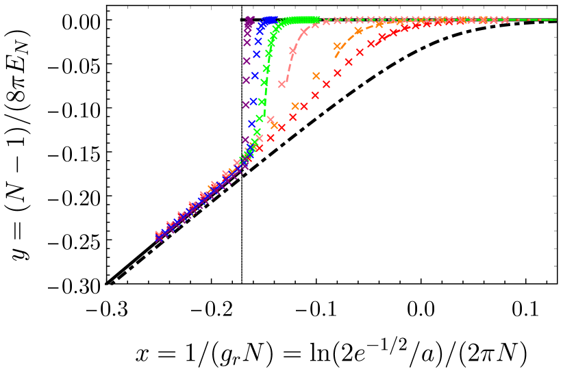
Figure 1: Inverse of the energy along the crossover from the weakly attractive (large negative $x$) to strongly attractive (large positive $x$) regimes. The cases of $N=2$ and $N=\infty$ are shown as the black dash-dotted curve and the piecewise linear black solid curve, respectively. The transition in the thermodynamic limit takes place at $x=-0.171$. The red, orange, pink, green, blue, and purple crosses are the Monte Carlo results, respectively, for $N=3,4,8,16,32$, and 128 bosons. The dashed curves show the flat-limit approximation Eq. (8).

In Fig. 1 we also show the energy obtained by solving the $N$-boson problem on a sphere by means of the diffusion and variational Monte Carlo methods which will be discussed in Sec. V. The dots in Fig. 1 stand for the DMC results for $N=3$ (red), $N=4$ (orange), $N=8$ (pink), $N=16$ (green), $N=32$ (blue), and $N=128$ (purple). The dashed curves correspond to Eq. (8) where the ratios $B_{N}/B_{2}$ are taken from Ref. [bazak2018, ]. These curves are valid when the soliton size $\sim 1/\sqrt{E_{N}}$ is much smaller than 1. Note that for large $N$ they become exact down to the transition point.

Let us now discuss how the cloud size changes as we vary the interaction strength. In Fig. 2 we show the root mean square (rms) separation between atoms as a function of the scattering length $a$ (rescaled by an $N$-dependent coefficient). The rms separation is calculated from the distribution of the three-dimensional (chord) distances between pairs of atoms. In the strongly interacting limit we are dealing with a localized and almost flat soliton, the size of which is proportional to $a$ [hammer2004, ]. Accordingly, we fit this linear dependence and rescale the horizontal axis to make the curves for different $N$ collapse to a single line. In the opposite weakly-interacting limit the distribution of atoms on our unit sphere is uniform and the rms size tends to $\sqrt{2}$. The way these two asymptotes are approached depends on $N$. We find that for $N\lesssim 10$ the derivatives of the curves are monotonic (within our precision) and for larger $N$ we start seeing a nonmonotonic structure, which eventually transforms into an abrupt change at a certain critical $a$. Our calculations are consistent with the scenario that there is a (narrow) crossing region where the exact ground state is a linear superposition of the soliton state and the uniform gas state. However, beginning with $N\sim 20$, our DMC scheme does not account for these effects. For $N=32$ and $128$ the DMC scheme predicts the energies and rms sizes of the two phases, but due to the importance sampling (necessary for these large $N$) the system gets stuck in one of the phases and cannot tunnel to the other. Neglecting this macroscopic tunneling one can say that the system undergoes a first-order phase transition (see the discussion in Sec. V). Comparing the data for $N=32$ and $N=128$ we observe that the rms size of the soliton at the transition indeed scales as $1/\sqrt{N}$.

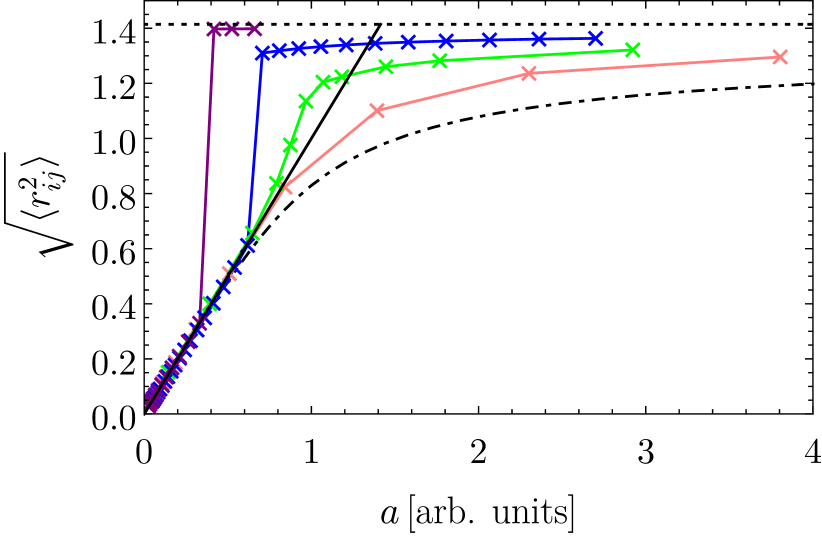
Figure 2: The rms separation versus $a$ for different values of $N$ as in Fig. 1 (we use the same color code). The interatomic distance is defined as the three-dimensional chord length. The horizontal axis is proportional to the scattering length $a$ rescaled by an $N$-dependent coefficient to make all curves tend to a unique line at small $a$. The nonmonotonic behavior of the slope of the curves for $N\geq 16$ signals the abruptly changing size in the vicinity of the gas-soliton transition.

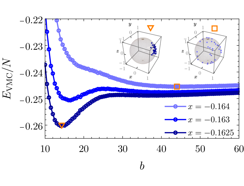
Figure 3: The variational energy per particle $E_{\text{VMC}}/N$ as a function of the localization parameter $b$ for $N=32$ and three close values of $x$ near the transition: for weak attraction (upper curve) there is a single minimum at large $b\gg 1$ physically corresponding to a uniform gas state, for strong attraction (bottom curve) the minimum is located at significantly smaller $b$ and describes a localized state, the middle curve shows the double minimum structure, typical for a first-order phase transition. The left and right insets show snapshots of particles’ coordinates in VMC simulation in the minumum of the lower curve (marked by triangle, $b=14$) and in the minimum of the upper curve (square, $b=44$), respectively.

V Monte Carlo for bosons on a sphere

To find the ground state of the $N$-boson problem numerically, we employ the variational (VMC) and diffusion (DMC) Monte Carlo methods, general details of which can be found, for instance, in Ref. [BoronatCasulleras1994, ]. The standard method has to be adapted to solving the Schrödinger equation on a sphere. As the variational (for VMC) and guiding (for DMC) wave function we take the Jastrow product

$$\Psi_{0}(\Omega_{1},\cdots,\Omega_{N})=\prod_{i<j}\chi(r_{ij}),$$ (9)

where $r_{ij}=|{\bf r}_{i}-{\bf r}_{j}|$ is the chord distance and ${\bf r}_{i}$ is the three-dimensional coordinate corresponding to the point $\Omega_{i}$ on the sphere. Expressing $\Psi$ in terms of chord distances regularizes the wave function and automatically takes care of the boundary condition when two atoms are on the opposite poles of the sphere ($\theta_{ij}=\pi$). For the Jastrow factor we choose $\chi(r)=K_{0}(2e^{-\gamma}r/a)e^{-r/b}$. With this choice $\Psi_{0}$ satisfies the Bethe-Peierls condition at short interparticle distances ($\theta_{ij}\approx r_{ij}\rightarrow 0$) as in the two-body case (see Sec. III) and we control the system size by tuning the variational parameter $b$.

In projection Monte Carlo methods, a first-order phase transition can be captured by imposing appropriate symmetry on the guiding wave functions. Probably, the most famous example of a zero-temperature quantum phase transition is that of the liquid-solid phase transition in ⁴He for which Monte Carlo calculations provide very good agreement with experiments [WhitlockCeperleyChesterKalos79, ]. The distinguishing feature between the two phases is the order parameter, with the liquid phase having translational invariance, which is instead broken in the solid phase, where particles get localized near the lattice sites. On the variational level, close to the phase transition point, the variational energy has two minima as a function of the localization size. One corresponds to a solid (localization size smaller than the mean inteparticle distance), while the other to a liquid (infinite localization size). The variational energy increases by going away from the minimum, so that each phase is stable against a weak perturbation, the phase with the lower energy being the ground state and the one with the higher energy being metastable. In contrast, in a second-order phase transition, only a single variational minimum exists, so that only one phase is stable at a time.

In our case, the variational parameter $b$ describes the degree of localization of the state and allows one to discriminate between the two phases. For a sufficiently large number of particles ($N\gtrsim 20$), indeed, we observe the double-minimum structure, characteristic of a first-order phase transition, see Fig. 3. The two minima are characterized by different values of $b$ and correspond, respectively, to the gas phase and to the localized soliton phase. The double minimum is observed in the variation energy in a narrow region of $x$ and the critical $x$ (when the two minima are degenerate) approaches the MF prediction $x\to-0.171$ as the number of particles is increased.

DMC method is based on solving the Schrödinger equation in imaginary time and it allows one to find the ground-state properties in the limit of long projection time. The convergence is significantly improved by using a guiding wave function (9) with values of optimal $b$ obtained by minimizing the variational energy. The procedure is in principle exact and is independent of the choice of the guiding function, as long as all relevant configurations are allowed. We find that for $N=32$ and 128 Eq. (9) with the variationally optimal values of $b$ well describes both the gas and soliton solutions, and for these particle numbers we do profit from importance sampling. However, since in the many-body configurational space the “gas” guiding function to a large extent excludes the “soliton” region and vice versa, in practice the diffusion process cannot account for the tunneling between the two phases. Quantitative description of the tunneling process in this case is an interesting future project going beyond the scope of this paper.

To mention a few technical details of our DMC scheme specific to the spherical geometry we find it convenient to work with particles’ three-dimensional coordinates ${\bf r}_{i}$ rather than with their polar angles and azimuths. In particular, the chord distance evaluation in this case is much more straightforward. The drift for particle $i$ is governed by the gradient of $\Psi_{0}$ with respect to ${\bf r}_{i}$ projected to the sphere surface. For the Jastrow product (9) this task reduces to calculating the projected gradient of $\chi$

$$\bar{\nabla}_{{\bf r}_{i}}\chi(|{\bf r}_{i}-{\bf r}_{j}|)=\chi^{\prime}(r_{ij})\frac{({\bf r}_{i}{\bf r}_{j}){\bf r}_{i}-{\bf r}_{j}}{r_{ij}}.$$ (10)

Neglecting finite time step corrections, we realize the diffusion and drift in a three-dimensional manner (as if the atoms were not confined), then projecting back to the sphere surface. The local energy can be expressed in terms of derivatives of $\chi$ by using

$$\hat{L}^{2}_{{\bf r}_{i}}\chi(|{\bf r}_{i}-{\bf r}_{j}|)=-\frac{1+{\bf r}_{i}{\bf r}_{j}}{2}\chi^{\prime\prime}(r_{ij})+\left(\frac{r_{ij}}{4}-\frac{{\bf r}_{i}{\bf r}_{j}}{r_{ij}}\right)\chi^{\prime}(r_{ij}).$$ (11)

Finally, we mention that another Monte Carlo method, path integral Monte Carlo, has recently been employed to study supersolidity of bosons on a sphere with soft-core and dipolar interactions at finite temperature [ciardi2023, ].

VI Conclusions

In this paper we address the problem of $N$ bosons on a spherical surface interacting via attractive zero-range potential and investigate how this system crosses over from the uniform gas state to the localized soliton state as one increases the attraction. Our main finding is that for sufficiently large $N$ we are essentially dealing with a first-order transition or, more precisely, a narrow avoided crossing between two states, which are significantly different in size and separated from each other by an energy barrier. On the other hand, for low values of $N$ the energy and rms size are smooth functions of the scattering length.

Our exact Monte Carlo calculations show that the change between these two regimes occurs when $N$ is roughly between $10$ and $20$. These relatively high values may be explained by a quantitatively weak geometry-induced breaking of the two-dimensional MF scaling invariance and, therefore, by a numerically small barrier. Indeed, in the MF approximation at $g=g_{c}$ the barrier equals $\Delta E_{\rm max}=0.0336N$ and we can compare it with the dipole mode frequency in the uniform phase $\epsilon_{1,1}=\sqrt{1-g_{c}/g_{d}}=0.262$. Here we have in mind that the dipole mode marks the initial “direction” for the system to tunnel towards the soliton side [Arovas, ]. We see that for large $N$ the barrier is indeed much higher than the dipole frequency, the tunneling is suppressed, and the gas-soliton transition looks discontinuos (from the practical viewpoint). By contrast, when $\Delta E_{\rm max}\lesssim\epsilon_{1,1}$ the role of the barrier is not very important and the crossover is smooth. Accordingly, the condition $\Delta E_{\rm max}=\epsilon_{1,1}$ leads to a characteristic atom number $N\approx 8$ where the crossover physics changes. This estimate is consistent with our Monte Carlo results.

We mention that the crossover scenario on a sphere is different from the previously solved model of attractive one-dimensional bosons on a ring where the gas-soliton transition is always continuous (no barrier), independent of $N$ [Lincoln, ,kanamoto2003, ]. In perspective it would therefore be interesting to study other geometries where the confinement can be used as a knob for controlling the crossover type and for elucidating the relative role of the space curvature, finite size, manifold topology, MF and beyond-MF terms. Being able to control the barrier and $N$ gives a way to prepare and probe superpositions of different macroscopic or mesoscopic quantum states.

Data Availability Statement

The data that support the findings of this study are available from the authors upon reasonable request.

Appendix A Derivation of Eq. (7)

A complementary manner of renormalizing the interaction is to expand the $N$-body energy in powers of $|g|\ll 1$ starting from the kinetic energy term in Eq. (1) as the unperturbed Hamiltonian. This standard perturbation theory works for finite $N$ and also predicts the nonpairwise energy contribution. For $N$ bosons on a unit sphere we obtain the ground-state energy up to terms of order $g^{3}$ in the form (see [PricoupenkoPetrov2021, ])

$$E_{N}=[g^{(1)}+g^{(2)}+g^{(3)}]\frac{N(N-1)}{2}+g_{3}\frac{N(N-1)(N-2)}{6},$$ (12)

where

$$g^{(1)}=V_{00}^{00}=\frac{g}{4\pi},$$ (13)

$$g^{(2)}=-\sum_{\nu}\frac{|V_{0\nu}^{0{\bar{\nu}}}|^{2}}{2\xi_{\nu}}=\left(\frac{g}{4\pi}\right)^{2}\left[\ln\frac{e^{1-2\gamma}}{l_{c}^{2}}+O(l_{c}^{-1})\right],$$ (14)

$$g^{(3)}= \sum_{\nu}\sum_{\nu^{\prime}}\frac{V_{0\nu^{\prime}}^{0\bar{\nu}^{\prime}}V_{\nu^{\prime}\nu}^{\bar{\nu}^{\prime}\bar{\nu}}V_{\nu 0}^{\bar{\nu}0}}{4\xi_{\nu}\xi_{\nu^{\prime}}}-V_{00}^{00}\sum_{\nu}\frac{|V_{0\nu}^{0{\bar{\nu}}}|^{2}}{4\xi_{\nu}^{2}}$$ (15)

$$= \left(\frac{g}{4\pi}\right)^{3}\left[\ln^{2}\frac{e^{1-2\gamma}}{l_{c}^{2}}-1+O(l_{c}^{-1})\right],$$

and

$$g_{3}=6\sum_{\nu}\frac{V_{0\nu}^{0\bar{\nu}}V_{\bar{\nu}0}^{0\bar{\nu}}V_{\nu 0}^{\bar{\nu}0}}{4\xi_{\nu}^{2}}=6\left(\frac{g}{4\pi}\right)^{3}[1+O(l_{c}^{-2})].$$ (16)

In Eqs. (14)-(16) $\nu=\{l,m\}$, $\nu^{\prime}=\{l^{\prime},m^{\prime}\}$, $\bar{\nu}=\{l,-m\}$, $\bar{\nu}^{\prime}=\{l^{\prime},-m^{\prime}\}$, $\sum_{\nu}=\sum_{l=1}^{l_{c}}\sum_{m=-l}^{l}$, and $\xi_{\nu}=l(l+1)/2$, where $l$ and $m$ correspond to the angular momentum and its projection for spherical harmonics. The quantities

$$V_{{\bm{\mu}}{\bm{\nu}}}^{{\bm{\zeta}}{\bm{\eta}}}=g\int\!d\Omega\psi^{*}_{{\bm{\zeta}}}(\Omega)\psi^{*}_{{\bm{\mu}}}(\Omega)\psi_{{\bm{\eta}}}(\Omega)\psi_{{\bm{\nu}}}(\Omega),$$ (17)

are the interaction matrix elements for two-body transitions from single-particle states $\mu$ and $\zeta$ to $\nu$ and $\eta$ and the corresponding wave functions are spherical harmonics. The last terms in Eqs. (14)-(16) are the final results obtained by summing over $\nu$ and $\nu^{\prime}$. The summation is facilitated by the fact that $V_{0\nu}^{0\bar{\nu}}=V_{\bar{\nu}0}^{0\bar{\nu}}=V_{\nu 0}^{\bar{\nu}0}=g/(4\pi)$. The more general matrix element $V_{\nu^{\prime}\nu}^{\bar{\nu}^{\prime}\bar{\nu}}$ in the first sum in Eq. (15) is not necessary to calculate explicitly. The result in this case is obtained by summing over the projections $m$ and $m^{\prime}$ and using the addition theorem for spherical harmonics. Finally, to arrive at Eq. (7) of the main text we rewrite the expansion (12) in powers of $g_{r}$ by using the relation $1/g=1/g_{r}+\ln(e^{-\gamma+1/2}/l_{c})/(2\pi)$ which follows from the definitions of $g$ and $g_{r}$ [see Eq. (5)]. Note that the cut-off dependence drops out.

References

- (1) R. Y. Chiao, E. Garmire, and C. H. Townes, Self-Trapping of Optical Beams, Phys. Rev. Lett. 13, 479 (1964).
- (2) B. Bakkali-Hassani, C. Maury, Y.-Q. Zou, É. Le Cerf, R. Saint-Jalm, P. C. M. Castilho, S. Nascimbene, J. Dalibard, and J. Beugnon, Realization of a Townes Soliton in a Two-Component Planar Bose Gas, Phys. Rev. Lett. 127, 023603 (2021).
- (3) C.-A. Chen and C.-L. Hung, Observation of Scale Invariance in Two-Dimensional Matter-Wave Townes Solitons, Phys. Rev. Lett. 127, 023604 (2021).
- (4) S. N. Vlasov, V. A. Petrishchev, and V. I. Talanov, Averaged description of wave beams in linear and nonlinear media, Izv. Vyssh. Uchebn. Zaved. Radiofiz. 14, 1353 (1971).
- (5) L. P. Pitaevskii, Dynamics of collapse of a confined Bose gas, Phys. Lett. A 221, 14 (1996).
- (6) L. P. Pitaevskii and A. Rosch, Breathing modes and hidden symmetry of trapped atoms in two dimensions, Phys. Rev. A 55, R853 (1997).
- (7) B. Bakkali-Hassani and J. Dalibard, Townes soliton and beyond: Non-miscible Bose mixtures in 2D, Proceedings of the International School of Physics "Enrico Fermi", Course 211 - Quantum Mixtures with Ultra-cold Atoms, July 2022, directors: Rudolf Grimm, Massimo Inguscio, Sandro Stringari.
- (8) H.-W. Hammer and D. T. Son, Universal properties of two-dimensional boson droplets, Phys. Rev. Lett. 93, 250408 (2004).
- (9) L. W. Bruch and J. A. Tjon, Binding of three identical bosons in two dimensions, Phys. Rev. A 19, 425 (1979).
- (10) S. K. Adhikari, A. Delfino, T. Frederico, I. D. Goldman, and L. Tomio, Efimov and Thomas effects and the model dependence of three-particle observables in two and three dimensions, Phys. Rev. A 37, 3666 (1988).
- (11) E. Nielsen, D. V. Fedorov, and A. S. Jensen, Three-body halos in two dimensions, Phys. Rev. A 56, 3287 (1997).
- (12) E. Nielsen, D. V. Fedorov, and A. S. Jensen, Structure and Occurrence of Three-Body Halos in Two Dimensions, Few-Body Systems 27, 15 (1999).
- (13) I. V. Brodsky, M. Yu. Kagan, A. V. Klaptsov, R. Combescot, and X. Leyronas, Exact diagrammatic approach for dimer-dimer scattering and bound states of three and four resonantly interacting particles, Phys. Rev. A 73, 032724 (2006).
- (14) O. I. Kartavtsev and A. V. Malykh, Universal low-energy properties of three two-dimensional bosons, Phys. Rev. A 74, 042506 (2006).
- (15) B. Bazak and D. S. Petrov, Energy of N two-dimensional bosons with zero-range interactions, New J. Phys. 20, 023045 (2018).
- (16) L. D. Carr, C. W. Clark, and W. P. Reinhardt, Stationary solutions of the one-dimensional nonlinear Schrödinger equation. II. Case of attractive nonlinearity, Phys. Rev. A 62, 063611 (2000).
- (17) R. Kanamoto, H. Saito, and M. Ueda, Quantum phase transition in one-dimensional Bose-Einstein condensates with attractive interactions, Phys. Rev. A 67, 013608 (2003).
- (18) R. A. Carollo, D. C. Aveline, B. Rhyno, S. Vishveshwara, C. Lannert, J. D. Murphree, E. R. Elliott, J. R. Williams, R. J. Thompson, and N. Lundblad, Observation of ultracold atomic bubbles in orbital microgravity, Nature 606, 281 (2022).
- (19) F. Jia, Z. Huang, L. Qiu, R. Zhou, Y. Yan, and D. Wang, Expansion Dynamics of a Shell-Shaped Bose-Einstein Condensate, Phys. Rev. Lett. 129, 243402 (2022).
- (20) Y. Guo, E. Mercado Gutierrez, D. Rey, T. Badr, A. Perrin, L. Longchambon, V. S. Bagnato, H. Perrin and R. Dubessy, Expansion of a quantum gas in a shell trap, New J. Phys. 24 093040 (2022).
- (21) A. Tononi and L. Salasnich, Low-dimensional quantum gases in curved geometries, Nat. Rev. Phys. 5, 398 (2023).
- (22) L. Amico, D. Anderson, M. Boshier, J.-P. Brantut, L.-C. Kwek, A. Minguzzi, and W. von Klitzing, Colloquium: Atomtronic circuits: From many-body physics to quantum technologies, Rev. Mod. Phys. 94, 041001 (2022).
- (23) A. Tononi, and L. Salasnich, Bose-Einstein Condensation on the Surface of a Sphere, Phys. Rev. Lett. 123, 160403 (2019).
- (24) A. Pricoupenko and D. S. Petrov, Higher-order effective interactions for bosons near a two-body zero crossing, Phys. Rev. A 103, 033326 (2021).
- (25) J. Boronat, and J. Casulleras, Monte Carlo analysis of an interatomic potential for He, Phys. Rev. B 49, 8920 (1994).
- (26) P. A. Whitlock, D. M. Ceperley, G. V. Chester, and M. H. Kalos, Properties of liquid and solid , Phys. Rev. B 19, 5598 (1979).
- (27) M. Ciardi, F. Cinti, G. Pellicane, S. Prestipino, Supersolid phases of bosonic particles in a bubble trap, arXiv:2303.06113 (2023).
- (28) A possible way of solving this tunneling problem is by using the instanton approach, see J. A. Freire and D. P. Arovas, Collapse of a Bose condensate with attractive interactions, Phys. Rev. A 59, 1461 (1999).