Ex-post Individually Rational Bayesian Persuasion

Abstract

The success of Bayesian persuasion relies on the key assumption that the sender will commit to a predetermined information disclosure policy (signaling scheme). However, in practice, it is usually difficult for the receiver to monitor whether the sender sticks to the disclosure policy, which makes the credibility of the sender’s disclosure policy questionable. The sender’s credibility is particularly tenuous when there are obvious deviations that benefit the sender. In this work, we identify such a deviation: the sender may be unwilling to send a signal that will lead to a less desirable outcome compared to no information disclosure. We thus propose the notion of ex-post individually rational (ex-post IR) Bayesian persuasion: after observing the state, the sender is never required to send a signal that will make the outcome worse off (compared to no information disclosure). An ex-post IR Bayesian persuasion policy is more likely to be truthfully followed by the sender, and thus more credible for the receiver. Our contribution is threefold. Firstly, we demonstrate that the optimal ex-post IR Bayesian persuasion policy can be efficiently computed through a linear program, while also offering geometric characterizations of this optimal policy. Second, we show that surprisingly, for non-trivial classes of games, the imposition of ex-post IR constraints does not affect the sender’s expected utility. Finally, we compare ex-post IR Bayesian persuasion to other information disclosure models that ensure different notions of credibility.

1 introduction

In the wake of the seminal works by [Rayo and Segal(2010)] and [Kamenica and Gentzkow(2011)], there has been a significant surge in research interest over the past decade concerning the design of optimal information disclosure policies, or Bayesian persuasion. In the most common formulation, Bayesian persuasion allows the sender to commit to sending any distribution of messages as a function of the state of the world. The assumption of a full commitment power, however, is not reasonable in many real-world scenarios. It is often impossible for the receiver to monitor whether the sender will stick to its signaling scheme, which makes the credibility of the sender’s signaling scheme questionable ([Nguyen and Tan(2021), Lipnowski et al.(2022), Lin and Liu(2022)]).

The sender’s credibility is particularly tenuous when there are obvious deviations that benefit the sender. Consider the following scenario. There is a credit reporting agency (the sender) recommending borrowers to a lender (the receiver). The lender makes loaning decisions based on the borrowers’ trustworthiness, i.e., whether the loan will be repaid. Suppose that the lender will reject the loan application if the probability of repayment is below $0.3$. The lender will issue a small loan if the probability is in $[0.3,1)$ and grant a huge loan if the probability is $1$. Suppose the lender’s prior about a borrower’s repayment probability is $0.5$, which means that without any recommendation from the sender, the lender will issue a small loan. Suppose the sender knows whether a borrower will repay the loan based on their credit history, and the sender can send a signal to the lender. The sender’s goal is to persuade the lender to approve loans. The sender’s utility is $0$ if the loan is rejected, $1$ if a small loan is approved, and $10$ if a huge loan is approved. Then the optimal Bayesian persuasion policy that maximizes the sender’s expected utility is to fully reveal whether the borrower will repay the loan, which gives an expected utility of $5$ supposing the prior probability of repayment is $0.5$. However, this optimal policy has its Achilles’ heel: the sender may hesitate to truthfully reveal low-credit borrowers who will not repay the loans. Because it will yield an outcome that is even worse than no information disclosure: the borrower will lose the small loan that is guaranteed when no information is disclosed. Consequently, the receiver might cast doubt on the credibility of the entire protocol: Why should I have faith that the sender will truthfully send a signal that will obviously hurt herself? In the absence of credibility, this policy may fail to effectively persuade the receiver.

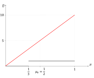
Figure 1: the utility curve of the sender. The red line is the concave closure of the utility curve. The optimal disclosure is truthfully reporting whether the receiver can repay ($\mu=1$) or not ($\mu=0$) and gives the sender a utility of $5$.

We thus consider the notion of ex-post individually rational (ex-post IR) Bayesian persuasion: after observing the state (the borrower’s trustworthiness), the sender is never required to send a signal that will make the outcome worse off (compared to no information disclosure). By mitigating the possibility of obvious deviations, an ex-post IR Bayesian persuasion policy is more likely to be truthfully followed by the sender, and thus more credible for the receiver. We provide three types of results about ex-post IR Bayesian persuasion.

First, we answer the question of how hard it is to compute the optimal signaling scheme in the ex-post IR Bayesian persuasion. We show that the optimal signaling scheme can still be solved by linear programming even if we add the ex-post IR constraints. In the original paper ([Kamenica and Gentzkow(2011)]) of Bayesian persuasion, they show the optimal signaling scheme can be characterized by the concave closure of the expected sender utility. Especially in the binary state case, the optimal signaling scheme can be read from the graph. Similarly, we provide the geometric characterization of the optimal ex-post IR signaling scheme and show how to read the optimal ex-post IR signaling scheme from the graph in the binary state cases.

Second, we explore when the ex-post IR constraints impose no cost to the sender. Not surprisingly, the ex-post IR constraints will decrease the optimal sender utility. A natural question is when the optimal sender utility in ex-post IR Bayesian persuasion is the same as the optimal sender utility in Bayesian persuasion. Inspired by the aforementioned geometric result, we give a complete geometric characterization in the binary state case (Theorem 4.1) of when there is no utility gap for sender between Bayesian persuasion and ex-post IR Bayesian persuasion. Our result links the optimal ex-post IR signaling scheme with the quasiconcave closure of the sender’s utility function. As a corollary of this, We show that our geometric result provides a more computationally efficient algorithm than simply running linear programming to determine whether there is no utility gap for the sender between Bayesian persuasion and ex-post IR Bayesian persuasion.

However, the geometric method doesn’t work in higher state dimensions. In general cases, our results are driven by real-world applications. We first consider the Bayesian persuasion in bilateral trade. We point out that the optimal signaling scheme is ex-post IR in the bilateral trade. Then we extend the bilateral trade to a general class of games we called trade-like games (Definition 4.2) and prove that the optimal signaling schemes of all trade-like games are ex-post IR. The bilateral trade is a special case of trade-like games. Besides, we show that the Bayesian persuasion in the first-price auction with reserve price is a special case of trade-like games. The other application we find is the Bayesian persuasion in the credence goods market, which is also widely studied in economic literature. We show when the optimal signaling scheme is ex-post IR in the credence goods market (Theorem 4.3). To prove this result, we introduce the notion of greedy signaling scheme. We show that in the credence goods market, the greedy signaling scheme is ex-post IR. Then the question of when there is no gap between the optimal signaling scheme and the optimal ex-post IR signaling scheme can be converted into the question of when there is no gap between the optimal signaling scheme and the optimal greedy signaling scheme. The latter question is answered by Theorem 4.3. Then we extend the credence goods market to a general class of games that satisfy two conditions called cyclical monotonicity and weak logarithmic supermodularity. We show that the greedy signaling schemes of this class of games are ex-post IR. Therefore, the gap between the optimal signaling scheme and the optimal ex-post IR signaling scheme can be controlled by the gap between the optimal signaling scheme and the optimal greedy signaling scheme.

Third, one may think that the ex-post IR Bayesian persuasion is also a Bayesian persuasion model with partial commitment. However, we show that this is not true if the sender’s preference over actions is not ordered (see 2.1), i.e. the sender utility of the optimal ex-post IR signaling scheme can even be worse than the utility of the cheap talk. Then with 2.1, we prove that the ex-post IR Bayesian persuasion is indeed a Bayesian persuasion model with partial commitment and we compare our model with a model called credible persuasion in [Lin and Liu(2022)], which also considers the credibility of the sender. We show that when the utility of the optimal ex-post IR signaling scheme is higher or lower than the utility of optimal credible persuasion. It deepens our understanding of the commitment power of the ex-post IR Bayesian persuasion.

The rest of the paper is organized as follows: Section 2 introduces the model of Bayesian persuasion and the definition of ex-post IR Bayesian persuasion. Section 3 provides results about the optimality of ex-post IR Bayesian persuasion in both algebraic and geometric views, which is similar to [Kamenica and Gentzkow(2011)]. Section 4 provides results of when there is no sender utility gap between the Bayesian persuasion and the ex-post IR Bayesian persuasion. Section 5 discusses the commitment power of the ex-post IR signaling scheme. All omitted proofs are in the appendix. The remainder of this introduction places the related literature.

1.1 Related literature

A substantial body of previous research has studied the credibility of the sender in Bayesian persuasion. They consider the notion of credibility in different ways, which are all different from ours. In the work of [Nguyen and Tan(2021)], the sender sends a signal to the receiver at some cost that depends on the signal and the realized world state, which makes the sender more credible. [Lipnowski et al.(2022)] considers the sender to communicate with the receiver through an intermediary which can be influenced by the sender with some probability. [Lin and Liu(2022)] characterize the notion of credibility by restricting the sender to only consider a marginal distribution of signals rather than the whole signaling scheme. There are more works about the limitation of the commitment power via repeated interactions ([Best and Quigley(2016), Mathevet et al.(2022)]), verifiable information ([Hart et al.(2017), Ben-Porath et al.(2019)]), information control ([Luo and Rozenas(2018)]), or mediation ([Salamanca(2021)]).

Our paper considers two applications of Bayesian persuasion: bilateral trade and credence goods market. The information transmission about these two applications has also been extensively studied in previous works. For the bilateral trade, [Ali et al.(2020)] considers the welfare of the sender (consumer) in both monopolistic and competitive markets, and [Glode et al.(2018)] considers the voluntary disclosure in the bilateral trade rather than the Bayesian persuasion. For the credence goods market, [Fong et al.(2014)] compares the market outcome with and without commitment and their model is extended by [Hu and Lei(2023)].

Technically, our work relies on two classical methods, which have also been successfully used in previous works. The first is quasiconcave closure. For example, [Lipnowski and Ravid(2020)] shows that in cheap talk, when the sender’s utility is state-independent, the optimal sender utility can be characterized by the quasiconcave closure of the sender’s utility function. The second is the greedy algorithm. For example, [Lucier and Syrgkanis(2015)] study mechanisms that use greedy allocation rules and show that all such mechanisms obtain a constant fraction of the optimal welfare.

2 Model

We introduce the standard Bayesian persuasion problem with finite actions and states, where a sender chooses a signal to reveal information to a receiver who then takes an action. The sender’s utility $v(a,\theta)$ and the receiver’s utility $u(a,\theta)$ depend on the receiver’s action $a\in A$ and the state of world $\theta\in\Theta$. Throughout this paper, we impose two assumptions. First, the sender has a preference over the actions regardless of the state. See 2.1 for the formal description. Second, there is no dominated action for the receiver, i.e. for any action $a$, there exists a posterior belief $\mu$ that $a$ is the best action for the receiver under $\mu$.

Assumption 2.1.

Let ${\mathchoice{\left|A\right|}{|A|}{|A|}{|A|}}=n$. The sender’s preference over action is $a_{1}\geq a_{2}\geq...\geq a_{n}$. In other words, for any $\theta\in\Theta$ and any $i,j\in[n]$ that $i\leq j$,

$$v(a_{i},\theta)\geq v(a_{j},\theta).$$

The sender and receiver share a common prior $\mu_{0}\in\Delta(\Theta)$ about the state. The sender commits to a signaling scheme $\phi$, which is a randomized mapping from the state to signals. Formally, the signaling scheme is defined as $\phi:\Theta\mapsto\Delta(S)$, where $S$ is the set of all possible signals. For convenience, let $\phi_{\theta}\in\Delta(S)$ be the conditional signal distribution when the state is $\theta\in\Theta$ and we denote by $\phi_{\theta}(s)$ the probability of sending signal $s\in S$ when the state is $\theta$. For ease of notation, we use $\phi$ to also denote the distribution over signals induced by the signaling scheme $\phi$ and the prior $\mu_{0}$ and denote $\phi(s)$ the probability of sending signal $s\in S$.

The interaction between the sender and the receiver goes on as follows:

1. the sender commits to a signaling scheme $\phi$ and the receiver observes it;

2. the sender observes a realized state of nature $\theta\sim\mu_{0}$;

3. the sender draws a signal $s\in S$ according to the distribution $\phi_{\theta}$ and sends it to the receiver;

4. the receiver observes the signal $s$ and updates her belief about the state according to the Bayes rule;

5. the receiver chooses an action that maximizes her expected utility.

The receiver’s posterior belief after seeing $s\in S$ is denoted by $\mu_{s}$. We have

$$\mu_{s}(\theta)=\frac{\mu_{0}(\theta)\phi_{\theta}(s)}{\phi(s)}.$$

For any posterior belief $\mu_{s}$, denote the receiver’s best response $a^{*}(\mu_{s})\in\operatorname*{arg\,max}_{a\in A}\sum_{\theta\in\Theta}u(a,\theta)\mu_{s}(\theta)$. For convenience, let the index of the best response under prior $a^{*}(\mu_{0})$ be $k^{*}$, i.e. $a^{*}(\mu_{0})=a_{k^{*}}$. As is customary in the literature, we assume that the receiver breaks ties in favor of the sender. The sender’s expected utility when sending $s$ will be equal to $\hat{v}(\mu_{s}):=\sum_{\theta\in\Theta}v\big{(}a^{*}(\mu_{s}),\theta\big{)}\mu_{s}(\theta)$. An outcome is a pair of the realized world state and the receiver’s action. Denote $\pi\in\Delta(A\times\Theta)$ the probability distribution of outcomes given the signaling scheme is $\phi$ and the prior $\mu_{0}$. We have

$$\pi(a,\theta)=\sum_{s\in S:a^{*}(\mu_{s})=a}\sum_{\theta\in\Theta}\phi_{\theta}(s)\mu_{0}(\theta).$$

.

Then, we introduce the definition of the ex-post individually rational (IR) signaling scheme.

Definition 2.1 (Ex-post individual rationality).

A signaling scheme $\phi$ is ex-post IR for the sender if for any state $\theta\in\Theta$ and any signal $s\in S$,

$$v(a^{*}(\mu_{s}),\theta)\geq v(a^{*}(\mu_{0}),\theta).$$ (1)

The definition of ex-post IR requires that compared to no communication, the sender will not regret sending the signal $s$ in any case. It can also mean that after the sender sees the state and draws a signal in Step 3, he will not hesitate to send the signal.

3 Warmup: optimal ex-post IR signaling schemes

It is well known that the optimal signaling scheme of a standard Bayesian persuasion problem with a finite number of actions and states can be solved by linear programming. In addition, the optimal expected Sender utility can be characterized by the concave closure of the expected Sender utility function $\hat{v}:\Delta(\theta)\mapsto\mathbb{R}$, which maps a posterior belief to the expected Sender utility.

In this section, we extend these two standard results to the setting of ex-post IR Bayesian persuasion. We first show that the ex-post IR constraints are linear, which implies that the optimal ex-post IR signaling scheme can also be solved by linear programming. Then we provide a concavefication characterization of the optimal ex-post IR signaling scheme.

3.1 Linear programming

The linear programming for Bayesian persuasion is

$$\max_{\pi}\sum_{a\in A}\sum_{\theta\in\Theta}v(a,\theta)\pi(a,\theta)$$

subject to

$$\sum_{\theta\in\Theta}(u(a,\theta)-u(a^{\prime},\theta))\pi(a,\theta)\leq 0\quad\forall a,a^{\prime}\in A$$ (2)

$$\sum_{a\in A}\pi(a,\theta)=\mu_{0}(\theta)\quad\forall\theta\in\Theta,$$ (3)

where Eq. 2 is the incentive compatible constraints for the Receiver and Eq. 3 is to make sure the signaling scheme is Bayes-plausible. To solve the optimal ex-post IR signaling scheme, we only need to add the following ex-post IR constraints

$$\pi(a,\theta)=0\quad\forall a\in A,\theta\in\Theta,u(a,\theta_{k})<u(a^{*}(\mu_{0}),\theta_{k}).$$ (4)

3.2 Concave closure

Let $V$ be the concave closure of the expected utility function $\hat{v}$.

Fact 3.1.

The value of the optimal signaling scheme is $V(\mu_{0})$. Sender benefits from persuasion if and only if $V(\mu_{0})>\hat{v}(\mu_{0})$

Now we consider Bayesian persuasion with ex-post IR constraints. Rather than compute the concave closure on the whole domain of posterior belief, we define a closure only on the posterior belief $\mu$ that $a^{*}(\mu)\geq a^{*}(\mu_{0})$. Let $A^{+}$ be the set of actions that Sender prefers them to $a^{*}(\mu_{0})$. Formally we have

$$\tilde{V}_{\textsc{ex-post}}(\mu_{0})=\max_{\tau\in\Delta\Delta(\Theta)}\{\sum_{\mu\in\mathrm{supp}(\tau)}\tau(\mu)\hat{v}(\mu):\sum_{\mu\in\mathrm{supp}(\tau)}\tau(\mu)\mu=\mu_{0},\quad a^{*}(\mu)\in A^{+},\forall\mu\in\mathrm{supp}(\tau)\}.$$ (5)

Theorem 3.1.

The value of the optimal ex-post IR signaling scheme is $V_{\textsc{ex-post}}(\mu_{0})$. Sender benefits from ex-post IR persuasion if and only if $V_{\textsc{ex-post}}(\mu_{0})>\hat{v}(\mu_{0})$.

The proof directly follows from the Eq. 5 and [Kamenica and Gentzkow(2011)], which is simple and omitted. Recall the example we mentioned in the introduction, Fig. 2 shows what the concave closure $V$ and the concave closure with ex-post IR constraints $V_{\textsc{ex-post}}$ looks like in this example.

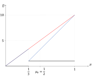
Figure 2: The black line is the piecewise function of expected Sender utility $\hat{v}$. The red line is the concave closure $V$. The blue line is the concave closure with ex-post IR constraints $V_{\textsc{ex-post}}$.

4 The effect of ex-post IR constraints

We have now understood how to compute the optimal ex-post IR signaling scheme and its concave closure representation. However, the impact of imposing the ex-post IR constraint is still not obvious. To compare the sender’s optimal signaling schemes with and without the ex-post IR constraints, we will need to solve two linear programs or find two concave closures. In this section, we examine how the ex-post IR requirement affects the sender’s expected utility and provide more explicit results. We zoom into the following question: when does the sender incur no cost due to the ex-post IR constraints? In other words, when will the optimal expected utility without ex-post IR constraints equal the optimal expected utility with ex-post IR constraints for the sender?

Firstly, in Section 4.1, we characterize the impact of the ex-post IR constraints by a simple function: smoothed quasiconcave closure. We show that the ex-post IR constraints impose no costs if and only smoothed quasiconcave closure is concave. This function is simple: it is built on connecting the left or right adjacent endpoints of the pieces of the quasiconcave closure of the sender’s expected utility function. See Theorem 4.1 for details. For the general cases, our results are driven by applications. We identify two non-trivial classes of games with real-world applications, demonstrating that ex-post IR constraints incur no costs in these games.

4.1 Geometric characterization in the binary state case

In this section, we consider a binary state set $\Theta=\{\theta_{1},\theta_{2}\}$ and a finite action set $A=\{a_{1},a_{2},...a_{n}\}$. In this case, It’s known that the optimal signaling scheme can be read from the concave closure of the sender’s expected utility function. In our paper, instead of considering the concave closure, we show how to determine whether there is a gap between the optimal signaling scheme and optimal ex-post IR signaling scheme through the quasiconcave closure of the sender’s expected utility function. In the binary state case, the sender’s expected utility function is a piecewise linear function, where each piece corresponds to an action representing the receiver’s best response. Formally, given ${\mathchoice{\left|\Theta\right|}{|\Theta|}{|\Theta|}{|\Theta|}}=2$ and ${\mathchoice{\left|A\right|}{|A|}{|A|}{|A|}}=n$, $\hat{v}$ is a one-dimensional piecewise function with $n$ pieces(segments) $S_{1},S_{2},...S_{n}$. Say $\mu(\theta_{1})$ is the independent variable of the function $\hat{v}$. The left endpoint and right endpoint of the segment $S_{i}$ are $L_{i}$ and $R_{i}$ respectively. The segment corresponding to the sender’s favorite action $a_{1}$ is $S_{i^{*}}$. And we use $a^{*}(S_{i})$ to represent the corresponding action of segment $S_{i}$. The threshold between segment $S_{i}$ and $S_{i+1}$ is $\alpha_{i}$ for $i=1,2,\cdots,n-1$. In other words, when $\mu(\theta_{1})\in(\alpha_{i-1},\alpha_{i})$, the best response for the receiver is $a^{*}(S_{i})$. When $\mu(\theta_{1})=\alpha_{i}$ for some $i$, the receiver breaks the tie in favor of the sender.

We first give two useful lemmas about the quasiconcave closure and the concave closure of the piecewise linear function. The first lemma says the quasiconcave closure of $\hat{v}$ is also a piecewise linear function and shows the monotonicity of the quasiconcave closure. We formally define the monotonicity of the piecewise function with respect to pieces.

Definition 4.1.

(monotone with respect to pieces) Consider a one-dimensional piecewise function $f$ with $n$ pieces $S_{1},S_{2},\cdots,S_{n}$. $f$ is increasing (decreasing) w.r.t pieces if for any function value in $S_{i}$ is smaller (larger) than any function value in $S_{j}$ for all $i,j\in[n]$ where $i<j$.

Then we formally present our lemma as follows.

Lemma 4.1.

Let $\overline{V}$ be the quasiconcave closure of the sender utility function $\hat{v}$. Then we have

1. The quasiconcave closure $\overline{V}$ is a piecewise linear function that $S_{i^{*}}$ is one segment of it.

2. The quasiconcave closure $\overline{V}$ is increasing w.r.t the pieces left to $S_{i^{*}}$ and decreasing w.r.t the pieces right to $S_{i^{*}}$.

The second lemma characterized the geometric property of the concave closure.

Lemma 4.2.

The concave closure V is a connecting segment

$$L_{i_{1}}L_{i_{2}}...L_{i_{k-1}}L_{i^{*}}R_{i^{*}}R_{i_{k}}...R_{i_{m}}$$

where $i_{1}<i_{2},..<i_{k-1}<i^{*}<i_{k}<...<i_{m}$.

Next, we present our main theorem in this section. It shows how to construct a smoothed quasiconcave closure directly from the quasiconcave closure and there is no gap between the optimal signaling scheme and optimal ex-post IR signaling scheme if and only if such a smoothed quasiconcave closure is concave.

Theorem 4.1.

Define a smoothed quasiconcave closure $\Gamma$ of $\hat{v}$ as follows:

1. $S_{i^{*}}$ is part of the closure.

2. On the left(right) of $S_{i^{*}}$, connect the left(right) endpoints of adjacent segments of $\overline{V}$ pairwise.

Then, the optimal signaling scheme is ex-post IR if and only if $\Gamma$ is concave.

Remark 4.1.

Given ${\mathchoice{\left|A\right|}{|A|}{|A|}{|A|}}=n$, Theorem 4.1 provides an algorithm to determine if the optimal signaling scheme is ex-post IR with the $O(n\log n)$ complexity, which is better than simply running a linear program to solve the optimal signaling scheme and check whether it is ex-post IR. In detail, we can sort each row of the receiver’s utility matrix according to the first entry of each row $u(a_{i},\theta_{1})$ for all $i\in[n]$ with complexity $O(nlogn)$. Then we can solve the sender’s expected utility function $\hat{v}$ with complexity $O(n)$. Because when the row of the receiver’s utility matrix is sorted, we can compute the threshold of each piece of $\hat{v}$ by inequality $\mu(\theta_{1})u(a_{i},\theta_{1})+\mu(\theta_{2})u(a_{i},\theta_{2})\leq\mu(\theta_{1})u(a_{i+1},\theta_{1})+\mu(\theta_{2})u(a_{i+1},\theta_{2})$ for all $1\leq i<n$. At last, we can construct $\Gamma$ and check whether it is concave in $O(n)$ complexity according to Theorem 4.1.

Intuitionally, to see why the concavity of the smoothed quasiconcave closure $\Gamma$ is crucial to whether the optimal signaling scheme is ex-post IR, let us first consider the part of concave disclosure $V$ that is on the left of the segment $S_{i^{*}}$. For some $1\leq j<k$, segment $L_{i_{j}}L_{i_{j+1}}$ connecting the left endpoint of $S_{i_{j}}$ and $S_{i_{j+1}}$. If there exists an index $i^{\prime}$ that $i_{j}<i^{\prime}<i_{j+1}$ and $a^{*}(S_{i_{j+1}})\geq a^{*}(S_{i^{\prime}})\geq a^{*}(S_{i_{j}})$, for any posterior belief $\mu$ that $a^{*}(\mu)=a^{*}(S_{i^{\prime}})$, the sender will send a signal that the receiver’s best response is a worse action $a^{*}(S_{i_{j}})$, which is not ex-post IR. That is if we connect one left endpoint of some segment $S_{i}$ to the left endpoints of its right closet segment $S_{n_{i}}$ whose corresponding action is better than $a^{*}(S_{i})$, $L_{i}L_{n_{i}}$ must be part of the concave closure $V$. Note that according to Lemma 4.1, the left pieces left to $S_{i^{*}}$ are increasing, we actually can prove when connecting the left endpoints of adjacent segments of $\overline{V}$, we are connecting one left endpoint of some segment $S_{i}$ to its right closet segment $S_{n_{i}}$. As for the part of concave disclosure $v$ that is on the right of the segment $L_{i^{*}}R_{i^{*}}$, we have a similar argument. Therefore, if the smoothed quasiconcave closure $\Gamma$ is not concave, there exists some $i$ that $L_{i}L_{n_{i}}$ or $R_{i}R_{n_{i}}$ is not part of the concave closure $V$, which means the optimal signaling scheme is not ex-post IR.

Finally, we provide a toy example for Theorem 4.1. Let one sender’s utility matrix and two receiver’s utility matrices be as follows.

$v$	$\theta=0$	$\theta=1$
$a=0$	$2$	$2$
$a=1$	$1$	$1$
$a=2$	$0$	$0$

$u$	$\theta=0$	$\theta=1$
$a=0$	$4$	$0$
$a=1$	$3$	$3$
$a=2$	$0$	$6$

$u$	$\theta=0$	$\theta=1$
$a=0$	$8$	$0$
$a=1$	$4$	$4$
$a=2$	$0$	$5$

Table 1: From left to right: the utility of the sender, the utility of the first receiver, the utility of the second receiver.

The sender faces two different receivers. The first receiver takes action $a=0$ when the posterior probability of $\theta$ being zero $\mu_{s}(0)\leq\frac{1}{2}$, takes action $a=1$ when $\frac{1}{2}\leq\mu_{s}(0)\leq\frac{3}{4}$ and takes action $a=2$ otherwise. The second receiver is slightly different in that its threshold of changing best response is $\frac{1}{5}$ (from $a=0$ to $a=1$) and $\frac{1}{2}$ (from $a=1$ to $a=2$). The figure of the sender’s expected utility function is as follows. In both cases, the sender’s expected utility function is a monotone function with respect to the posterior belief’s probability of being $\theta_{1}$. Therefore, the quasiconcave closure of the sender’s expected utility function is itself. In the first case, when the prior is $\frac{1}{2}\leq\mu_{0}(0)\leq\frac{3}{4}$, the optimal disclosure policy is divided the prior into two posterior $s_{1},s_{2}$, $\mu_{s_{1}}(0)=0$ and $\mu_{s_{2}}(0)=\frac{3}{4}$ with the best response being $a=2$ and $a=0$ respectively. So the sender is worse off under $s_{2}$. In contrast, the sender is never worse off under any signal of the optimal disclosure policy. The difference is that the smoothed quasiconcave closure $\Gamma$ is not concave in the first case but is concave in the second case.

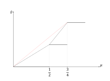
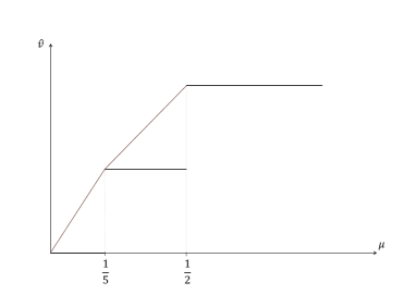
Figure 3: Left: the expected utility curve of the sender when facing the first receiver, the smoothed quasiconcave closure $\Gamma$ (black, dotted) is not concave and not same as the concave closure (red, solid). right: the expected utility curve of the sender when facing the second receiver, the smoothed quasiconcave closure $\Gamma$ (black, dotted) is concave and the same as the concave closure (red, solid).

4.2 No gap in the bilateral trade market

In this section, we introduce the Bayesian persuasion model between a monopolistic seller and a consumer that was studied in [Bergemann et al.(2015), Glode et al.(2018)]. We point out that the optimal signaling scheme is ex-post IR in this setting.

Bilateral trade A monopolist sells to a consumer, who has $n$ possible values $\theta\in\Theta$: $0<\theta_{1}<\theta_{2}<...<\theta_{n}$. The monopolist sets a price $a\in A$ and the trade only happens when the consumer’s value is higher than the price. The monopolist will not set a price between any two closest values $\theta_{i}$ and $\theta_{i+1}$ for some $i$ because the monopolist can increase the price to $\theta_{i+1}$ without decreasing the probability of making a deal. Therefore, we can let $A=\Theta$ without loss of generality. The monopolist doesn’t know the consumer’s value but shares a prior $\mu_{0}$ of the value with the consumer. Before the trade, the consumer commits to a signaling scheme. Then the monopolist sets the price according to the posterior belief. The utility of the consumer is $v(a,\theta)=(\theta-a)\cdot\mathbbm{1}_{\theta\geq a}$ and the utility of the monopolist is $u(a,\theta)=a\cdot\mathbbm{1}_{\theta\geq a}$.

Fact 4.1.

[Bergemann et al.(2015)] In the persuasion model of bilateral trade, the optimal signaling scheme of the consumer is ex-post IR.

$v$	$\theta_{1}$	$\theta_{2}$	$\cdots$	$\theta_{n}$
$a_{1}(=\theta_{1})$	$\theta_{1}$	$\theta_{1}$	$\cdots$	$\theta_{1}$
$a_{2}$	$0$	$\theta_{2}$	$\cdots$	$\theta_{2}$
$\cdots$	$\cdots$	$\cdots$	$\cdots$	$\theta_{n-1}$
$a_{n}$	$0$	$0$	$\cdots$	$\theta_{n}$

Table 2: The utility of receiver in the bilateral trade

Since a Bayesian persuasion instance is determined and only determined by the sender’s and the receiver’s utility function $v,u$. We use a pair $(v,u)$ to denote a Bayesian persuasion instance, also called game for short. The bilateral trade game satisfies the following properties: (1) the utility of the receiver is upper-triangular (2)the non-zero part corresponding columns of the receiver utility is increasing from top to bottom (3) the sum of the non-zero part corresponding columns of the sender utility and the receiver utility is a constant. We extend the bilateral trade game to a general class of games called trade-like games. As long as a game satisfies the aforementioned properties, it is a trade-like game (see Definition 4.2). We show that the optimal signaling scheme of any trade-like game is ex-post IR.

Definition 4.2.

(trade-like game) A game (v, u) is a trade-like game if the following conditions hold

1. u is upper-triangular and non-negative: $u(a_{i},\theta_{k})\geq 0$ for all $i,k\in[n]$ and $u(a_{i},\theta_{k})=0$ if $i>k$.

2. the non-zero part corresponding columns of the receiver utility is increasing: $u(a_{i},\theta_{k})\leq u(a_{j},\theta_{k})$ for all $i,j,k\in[n]$ that $i<j\leq k$.

3. $v(a_{i},\theta_{k})+u(a_{i},\theta_{k})=c_{k}$ where $c_{k}$ is a positive constant for all $i,k\in[n]$ that $i\leq k$.

These three conditions generally hold in a trade-like setting, where there is a seller and a buyer. When the seller sets a price that is higher than the buyer’s value, the buyer will not buy. Therefore, the first and the second condition holds. And when the trade happens, the total utility of the buyer and the seller should be the buyer’s value. Then the third condition holds. We have that as long as the game is a trade-like game, the optimal signaling scheme is ex-post IR.

Theorem 4.2.

For all trade-like games, there exists an optimal signaling scheme that is ex-post IR.

To illustrate the idea of the proof, we first provide a lemma about the property of the receiver’s best response.

Lemma 4.3.

Assume the utility matrix $u$ is upper-triangular and non-negative, for any subset $S\subset[n]$, there exists a posterior belief $\mu_{S}$ that

• the support of $\mu_{S}$ is $\mu_{S}(\theta_{k})$ for all $k\in S$.

• the best response set of the receiver under $\mu_{S}$ is $a_{k}$ for all $k\in S$.

Based on how the receiver best responds, we show that there is a specific structure of ex-post IR signaling schemes. The specific structure is as follows. We start from the prior $\mu_{0}$ and let $S_{0}=\{1,2,...,n\}$. In the first step, we compute a posterior belief $\mu_{S_{0}}$ that is indifferent among $\theta_{i}$ for all $i\in S_{0}$, namely, all the states. Then we subtract certain proportions of $\mu_{S_{0}}$ from $\mu$ until some supports of $\mu_{0}$ become zero. Slightly abusing the notation, we still use $\mu_{0}$ to be the vector after the subtraction and let $S_{1}$ be the set of indexes that $\mu_{0}$ has support on their corresponding state. In the following step t=2,3,…, we repeat this process. That is, we compute a posterior belief $\mu_{t}$ that is indifferent among $\theta_{i}$ for all $i\in S_{t-1}$ and subtract it from $\mu_{0}$. This procedure will stop in finite steps because at least one component of $\mu_{0}$ becomes zero in each step and there are finite $n$ components. We will show that the last component becoming zero is $\theta_{i^{*}}$ under which the best response $a_{i^{*}}$ is also the best response under the prior $\mu_{0}$. Therefore, we divide the prior into several posterior beliefs that $a_{i^{*}}$ is one of the best responses under each of them. The sender hence always enjoys a utility better than the utility under the prior, which means the signaling scheme is ex-post IR. We then complete the proof by showing that such a signaling scheme is optimal. The detailed proof is in Section A.2. At last, we show that Theorem 4.2 allows us to include more applications where the optimal signaling scheme is ex-post IR. The following example is about the Bayesian persuasion problem in the first price auction (FPA) with a reserve price. We show that this game is a trade-like game and hence the optimal signaling scheme is ex-post IR.

Example 4.1.

Consider the first-price auction with multiple bidders, when we set reserve prices, we only care about the maximum bid. It is useful to abstract bidders in the auction as a single ”mega-bidder” whose value is the maximum of values and who always bids the maximum of all bids (see [Feng et al.(2020)]). Now we can consider the pricing problem between the seller(receiver) and the representative winning bidder(sender). The state is the value of the bidder $\theta_{1}\leq\theta_{2}\leq...\leq\theta_{n}$. The action is the reserve price set by the seller. Notice that the seller will never set a reserve price between some $\theta_{i-1}$ and $\theta_{i}$ because he has the incentive to increase the reserve price to exact $\theta_{i}$. Then the receiver has exactly n actions $a_{1},...,a_{n}$ which $a_{i}$ is setting the reserve price at $\theta_{i}$. The bidder’s bidding function $b(r,v)$, which is determined by the reserve price $r$ and the bidder’s value $v$, is increasing w.r.t to the reserve price $r$. The payoff matrix of the sender and receiver are Table 3 and Table 4.

$v$	$\theta_{1}$	$\theta_{2}$	$\cdots$	$\theta_{n}$
$a_{1}(=\theta_{1})$	0	$\theta_{2}-b(\theta_{1},\theta_{2})$	$\cdots$	$\theta_{n}-b(\theta_{1},\theta_{n})$
$a_{2}$	$0$	$0$	$\cdots$	$\theta_{n}-b(\theta_{2},\theta_{n})$
$\cdots$	$\cdots$	$\cdots$	$\cdots$	$\theta_{n}-b(\theta_{n-1},\theta_{n})$
$a_{n}$	$0$	$0$	$\cdots$	$0$

Table 3: The utility of sender in the FPA

$v$	$\theta_{1}$	$\theta_{2}$	$\cdots$	$\theta_{n}$
$a_{1}(=\theta_{1})$	$b(\theta_{1},\theta_{1})$	$b(\theta_{1},\theta_{2})$	$\cdots$	$b(\theta_{1},\theta_{n})$
$a_{2}$	$0$	$b(\theta_{2},\theta_{2})$	$\cdots$	$b(\theta_{2},\theta_{n})$
$\cdots$	$\cdots$	$\cdots$	$\cdots$	$b(\theta_{n-1},\theta_{n})$
$a_{n}$	$0$	$0$	$\cdots$	$b(\theta_{n},\theta_{n})$

Table 4: The utility of receiver in the FPA

4.3 No gap in the credence goods market

In this section, we prove when there is no gap led by ex-post IR constraints in the credence goods market. In the credence goods market, the gap is controlled by the gap between the optimal signaling scheme and an optimal greedy signaling scheme. We extend the credence goods market to a general class of games in which the gap led by ex-post IR constraints can be controlled in the same way.

First, we give a brief introduction to the credence goods market. A credence good is a product or service whose qualities or appropriateness are hard to evaluate for clients even after consumption. A credence good is a product or service whose qualities or appropriateness are hard to evaluate for consumers even after consumption. Common examples of credence goods include medical services, automobile repairs, and financial advice. For instance, patients who receive expensive medical treatments may struggle to know their value post-recovery. Car owners may question the necessity of replacing expensive parts of cars during repairs. Additionally, investors with limited financial know-how may remain unsure about the suitability of a financial product even after realizing returns. On the flip side, expert sellers frequently possess superior insights into the appropriateness of credence goods and can use this knowledge to their advantage.

The persuasion model The client has a problem with an uncertain type which is drawn from a set $\Theta=\{\theta_{1},...,\theta_{n}\}$ according to the common prior $\mu_{0}$. The expert provides n different treatments $A=\{a_{1},a_{2},...,a_{n}\}$. A treatment $a_{i}$ can solve the problem of $\theta_{j}$ if and only if $i\geq j$. $a_{n}$ is a panacea that fully resolves all problems. The cost of each treatment $a_{i}$ for the expert is $c_{i}$. For each treatment $a_{i}$, the client needs to pay the price $p_{i}$ to the expert. We assume that the price of more effective action is higher: $p_{1}\leq p_{2}\leq\cdots p_{n}$. If the problem remains unsolved, the client will suffer an extra disutility $l$. The utility of the receiver, namely client is $u(a_{i},\theta_{j})=-p_{i}-l\cdot\mathbbm{1}_{i<j}$. Without loss of generality, we add a sufficiently large constant $c$ on the utility of the receiver to keep it positive, let $r_{i}=c-p_{i}$. The receiver’s utility is $u(a_{i},\theta_{j})=r_{i}-l\cdot\mathbbm{1}_{i<j}$. We assume the expert is altruistic, which means his utility doesn’t contradict the client’s utility. This assumption is plausible according to [Farukh et al.(2020)]. Formally, we denote the cost of each treatment as $c_{i}$ for all $i\in[n]$ and the sender utility is $v(a_{i},\theta_{j})=p_{i}-c_{i}\triangleq s_{i}$. We have $p_{1}-c_{1}\geq p_{2}-c_{2}\cdots\geq p_{n}-c_{n}$.

Theorem 4.3.

In the persuasion model of the credence goods market, the optimal signaling scheme is ex-post IR if

$$(1-\frac{l}{l-(r_{i+1}-r_{n})})s_{i}\geq s_{i+1}$$

for all i that $1\leq i<n$.

Technically, our result relies on a notion of greedy algorithm. In detail, when the sender’s preference over actions is $a_{1}\geq a_{2}\geq...\geq a_{n}$. A natural greedy idea to compute the signaling scheme goes as follows. Given the prior $\mu_{0}$, we compute a posterior belief $\mu_{1}$ that maximizes the probability of taking action $a_{1}$ and subtract it from the prior. Note that this can be computed by simply running linear programming. Then compute the posterior belief that maximizes the probability of taking action $a_{2},...,a_{n}$ respectively. Formally, we provide the algorithm (see Algorithm 1) to solve the greedy signaling scheme. We can prove that in the credence market, the greedy signaling scheme is ex-post IR. Furthermore, our condition in Theorem 4.3 characterizes when the greedy signaling scheme is optimal.Combining two results together, we know such an optimal signaling scheme is ex-post IR.

The game of credence market satisfies two properties we term as cyclically monotonicity and weak logarithmic supermodularity for the receiver’s utility. The word ”weak” means that the logarithmic supermodularity doesn’t need to hold for the diagonal elements. Formally, we have

Definition 4.3.

(cyclical monotonicity) A utility function u is cyclically monotone if for all $i,j,k\in[n]$ that $i<j$

$$u(a_{k-1+i},\theta_{k})\geq u(a_{k-1+j},\theta_{k})$$

where $a_{k-1+i}\equiv a_{(k-1+i)\mathrm{mod}n}$.

Definition 4.4.

(weak logarithmic supermodularity) A utility function u is weakly supermodular in logarithmic form if $\frac{u(a_{i},\theta_{k})}{u(a_{j},\theta_{k})}\geq\frac{u(a_{i},\theta_{k+1})}{u(a_{j},\theta_{k+1})}\quad\forall 1\leq i<j,k<n,j\neq k$.

Then we extend the game of credence market to a general class of games. Our extension says that as long as a game satisfies cyclical monotonicity and weak supermodularity in logarithmic form, the greedy signaling scheme is ex-post IR. Therefore, the greedy signaling scheme is ex-post IR for any game in this class. As a corollary, the gap between the gap between the optimal signaling scheme and the optimal ex-post IR signaling scheme can be upper bound by the gap between the optimal signaling scheme and the greedy signaling scheme.

Theorem 4.4.

The greedy signaling scheme is ex-post IR if $u$ is cyclically monotone and weakly supermodular in logarithmic form.

The proof idea is as follows. To prove the greedy signaling scheme is ex-post IR is equivalent to proving GS will stop in $k^{*}$ steps. Now suppose the algorithm is in the first step. Let us consider the linear programming $LP_{1}$. Denote the jth constraint of Eq. 6 that means incentive compatibility as $\mathrm{IC}_{j}$ and the jth constraint of Eq. 7 as $\mathrm{Budget}_{j}$. We will prove that for any $j>k^{*}$, at least one of $\mathrm{IC}_{j}$ and $\mathrm{Budget}_{i}$. If $\mathrm{Budget}_{j}$ holds, after running $LP_{i}$ and updating $\mu$, we have $\mu(\theta_{j})=0$. If $\mathrm{IC}_{j}$ holds, $a_{1}$ and $a_{j}$ are both best response under $\pi(a_{1},\cdot)$. In both cases, we will show $a_{k^{*}}$ is a better action than $a_{j}$ under $\mu-\pi_{1}$. As the Algorithm 1 goes, the best response of $\mu$ will not get worse for the sender. At some time, when running $LP_{i}$ for some $i\leq k^{*}$, we will have the best response of $\mu$ is $a_{i}$. The algorithm will use up all the ”budget” (see Remark 4.2) due to greediness and the algorithm stops.

Corollary 4.1.

If a game $(v,u)$ satisfies that $u$ is cyclically monotone and weakly supermodular in logarithmic form, for any prior $\mu_{0}$, we have

$$V(\mu_{0})-V_{\textsc{ex-post}}(\mu_{0})\leq V(\mu_{0})-V_{\textsc{greedy}}(\mu_{0})$$

where $V_{\textsc{greedy}}(\mu_{0})$ is the sender’s utility under the optimal greedy signaling scheme.

In algorithm analysis, the greedy algorithm by nature has a close link with the optimal solution. We believe that Corollary 4.1 will be useful in finding more games where there is no gap between the optimal signaling schemes with and without ex-post IR constraints.

Algorithm 1 GS: greedy signaling scheme

0:  prior $\mu_{0}=(\mu_{0}(\theta_{1}),...,\mu_{0}(\theta_{n}))$

  $\pi\leftarrow 0$

  $\mu\leftarrow\mu_{0}$

  while $\mu\neq 0$ do

     solve $\pi(a_{i},\cdot)$ by $LP_{i}$ so that the probability of taking action $a_{i}$ is maximized

     $\mu\leftarrow\mu-\pi(a_{i},\cdot)$

  end while

  a feasible outcome $\pi(a,\theta)$

where $LP_{i}$ is

$$\max\sum_{k}\pi(a_{i},\theta_{k})$$

subject to

$$\sum_{k}(u(a_{j},\theta_{k})-u(a_{i},\theta_{k}))\pi(a_{i},\theta_{k})\leq 0\quad\forall j\in[n]$$ (6)

$$\pi(a_{i},\theta_{k})\leq\mu(\theta_{k})\quad\forall k\in[n]$$ (7)

Remark 4.2.

For convenience, we slightly abuse notation by using $\mu$ as the belief that is not normalized to 1. In this section, it will be better to treat the prior $\mu_{0}$ as an initial multidimensional ”budget” and after each step of the greedy algorithm, each dimension of the budget decreases. The algorithm stops until all the budget is used up.

5 Comparison of commitment power

The power of commitment is reflected by the optimal sender utility that can be achieved. Typically, the stronger the commitment power is, the higher optimal sender utility can be achieved. In many previous works about Bayesian persuasion with partial commitment, such as [Min(2021), Lin and Liu(2022)], the optimal sender utility achieved by their model is between the Bayesian persuasion and cheap talk. Therefore, it is natural to compare the commitment power of our ex-post IR Bayesian persuasion with the commitment power of Bayesian persuasion and cheap talk. Besides, since our model considers the credibility of the sender, we compare the ex-post IR Bayesian persuasion to another model called credible persuasion in the paper by [Lin and Liu(2022)], which also considers the credibility of the sender.

Totally we will compare four information transmission models: Bayesian persuasion, ex-post IR Bayesian persuasion, credible persuasion, and cheap talk. Given the sender’s utility $v$, receiver’s utility $u$, and prior $\mu_{0}$, we denote the optimal sender utility gained in these four models as $V_{\textsc{BP}}$, $V_{\textsc{expost}}$, $V_{\textsc{credible}}$, $V_{\textsc{cheap}}$. We formally give the definition that the optimal sender utility achieved in one information transmission model is better than the optimal sender utility achieved in another information transmission model.

Definition 5.1.

Consider two information transmission model $X,Y$. If for any $v,u,\mu_{0}$, we have $V_{X}(\mu_{0})\geq V_{Y}(\mu_{0})$, we say the optimal sender utility achieved in $X$ is better than the optimal sender utility achieved in $Y$, which is denoted by $V_{X}\succeq V_{Y}$.

At first glance, the reader may think ex-post IR Bayesian persuasion is also between Bayesian persuasion and cheap talk. However, we can give an example that if 2.1 doesn’t hold, the optimal sender utility achieved by the ex-post IR Bayesian can be worse than the utility achieved by the cheap talk. In other words, there exists $v,u,\mu_{0}$ such that $V^{\mathrm{cheaptalk}}(\mu_{0})>V^{\mathrm{expostBP}}(\mu_{0})$. Our example is based on the following Lemma 5.1 that shows when there is no sender utility gap between the Bayesian persuasion and cheap talk.

Lemma 5.1.

[Lipnowski(2020)] If the expected sender utility $\hat{v}$ is continuous, for any $\mu_{0}$, $V^{\mathrm{BP}}(\mu_{0})=V^{\mathrm{Cheaptalk}}(\mu_{0})$.

Then we can construct an example that the optimal sender utility gained by cheap talk is the same as the optimal sender utility gained by the Bayesian persuasion while the optimal sender utility gained by ex-post IR Bayesian persuasion is strictly smaller than the optimal sender utility gained by the Bayesian persuasion.

Example 5.1.

Consider $A=\{a_{1},a_{2},a_{3},a_{4},a_{5}\}$ and $\theta=\{\theta_{1},\theta_{2}\}$, the sender utility $v$ and the receiver utility $u$ is as follows.

	$\theta_{1}$	$\theta_{2}$
$a_{1}$	10	0
$a_{2}$	-2	3
$a_{3}$	1	1
$a_{4}$	3	-2
$a_{5}$	0	10

	$\theta_{1}$	$\theta_{2}$
$a_{1}$	-4	21
$a_{2}$	0	20
$a_{3}$	12	12
$a_{4}$	20	0
$a_{5}$	21	-4

Table 5: the utility of sender and receiver

For any $\mu_{0}$ that $\mu_{0}(\theta_{1})\in(\frac{2}{5},\frac{3}{5})$, $a^{*}(\mu_{0})=a_{3}$. The optimal ex-post IR signaling scheme is no communication and $V^{\mathrm{expostBP}}(\mu_{0})=1$. $\hat{v}$ is continuous so the optimal sender utility of cheap talk is equal to the optimal sender utility of Bayesian persuasion. We have $V^{\mathrm{Cheaptalk}}(\mu_{0})=2$. Therefore, $V^{\mathrm{Cheaptalk}}(\mu_{0})>V^{\mathrm{expostBP}}(\mu_{0})$ for any $\mu_{0}\in(\frac{2}{5},\frac{3}{5})$.

Next we assume 2.1 hold and we will show that $V^{\mathrm{expostBP}}\succeq V^{\mathrm{Cheaptalk}}$. Therefore, we can also put our model in the scope of Bayesian persuasion with partial commitment and compare it to credible persuasion. We give a brief introduction to the credible persuasion.

Credible persuasion The interaction between the sender and the receiver goes on as follows:

1. sender chooses a signaling scheme $\phi$. Different from the Bayesian persuasion, the receiver can not observe the signaling scheme;

2. sender observes a realized state of nature $\theta\sim\mu_{0}$;

3. sender draws a signal $s\in S$ according to the distribution $\phi_{\theta}$ and sends it to the receiver;

4. receiver observes the signal $s$. Different from the Bayesian persuasion, the receiver can also observe the distribution of signals induced by $\phi$.

5. The receiver chooses an action based on both the signal $s$ and the distribution of signals.

Their notion of credibility is captured by the restriction that the receiver can only see the distribution of the signal induced by a signaling scheme $\phi$ instead of the whole signaling scheme. The receiver can not distinguish the signaling schemes that induce the same distribution of signals as $\phi$. Denote the set of such signaling schemes $D(\phi)$. They require when the sender chooses a signaling scheme $\phi$, it has no profitable deviation in $D(\phi)$.

We show that both ex-post IR Bayesian persuasion and credible persuasion are partial commitment models between Bayesian persuasion and cheap talk. Then we show that in some games, the commitment power of ex-post IR Bayesian persuasion is stronger than the commitment power of credible persuasion. While in some other games, the commitment power of credible persuasion is stronger than the commitment power of ex-post IR Bayesian persuasion. The results are summarized in Theorem 5.1.

Theorem 5.1.

The rank of the optimal sender’s utility is as follows:

1. $V^{\mathrm{BP}}\succeq V^{\mathrm{credible}},V^{\mathrm{expostBP}}\succeq V^{\mathrm{cheaptalk}}$.

2. There exists $v,u$ such that for any $\mu_{0}$,

   $$V^{\mathrm{credible}}(\mu_{0})\geq V^{\mathrm{expostBP}}(\mu_{0}).$$

3. There exists $v,u$ such that for any $\mu_{0}$,

   $$V^{\mathrm{expostBP}}(\mu_{0})\geq V^{\mathrm{credible}}(\mu_{0}).$$

The first part of Theorem 5.1 that ex-post IR Bayesian persuasion and credible persuasion are partial commitment models based on the solution concept of cheap talk. The second part of Theorem 5.1 that the commitment power of ex-post IR Bayesian persuasion and credible persuasion differs in different cases based on a series of lemma that show when the optimal sender utility of ex-post IR Bayesian persuasion or credible persuasion is the same as the optimal sender utility of Bayesian persuasion. Then we can construct examples when one model’s optimal sender utility is equal to the optimal sender utility of Bayesian persuasion and the other model’s optimal sender utility is strictly smaller than the optimal sender utility of Bayesian persuasion.

Appendix A Missing proofs from Section 4

A.1 Missing Proofs from Section 4.1

Proof of Lemma 4.1

Proof.

In the binary state case, we slightly abuse notation by using $\mu$ to represent $\mu(\theta_{1})$. Consider any possible linear combination $\mu=\lambda\mu_{1}+(1-\lambda)\mu_{2}$ that $\lambda$ is a real number in $[0,1]$. According to the definition of quasiconcave closure, we have

$$\overline{V}(\mu)\geq\min\{\overline{V}(\mu_{1}),\overline{V}(\mu_{2})\}\geq\min\{\hat{v}(\mu_{1}),\hat{v}(\mu_{2})\}.$$

On one hand, we can assume $\mu_{1}\leq\mu\leq\mu_{2}$ without loss of generality. Combining the inequalities led by all linear combinations, we have $\overline{V}(\mu)\geq\min\{\max_{\mu_{1}:\mu_{1}\leq\mu}\hat{v}(\mu_{1}),\max_{\mu_{2}:\mu_{2}>\mu}\hat{v}(\mu_{2})\}$ On the other hand, if a closure of $\hat{v}$ satisfies its value of $\mu$ is $\min\{\max_{\mu_{1}:\mu_{1}\leq\mu}\hat{v}(\mu_{1}),\max_{\mu_{2}:\mu_{2}>\mu}\hat{v}(\mu_{2})\}$ for all $\mu\in[0,1]$, it is indeed quasiconcave. Therefore, we have

$$\overline{V}(\mu)=\min\{\max_{\mu_{1}:\mu_{1}\leq\mu}\hat{v}(\mu_{1}),\max_{\mu_{2}:\mu_{2}>\mu}\hat{v}(\mu_{2})\}.$$ (8)

Then $\overline{V}$ is a linear piecewise function because $\hat{v}$ is a linear piecewise function.

Now let us prove that $S_{i^{*}}$ is one piece of $\overline{V}$. According to $a^{*}(S_{i^{*}})=a_{1}$ and 2.1, we have $\hat{v}(\mu)>\hat{v}(\mu^{\prime})$ for all $\mu\in[\alpha_{i^{*}-1},\alpha_{i^{*}}]$ and $\mu^{\prime}\notin[\alpha_{i^{*}-1},\alpha_{i^{*}}].$ Then $\overline{V}(\mu)=\hat{v}(\mu)$ for all $\mu\in[\alpha_{i^{*}-1},\alpha_{i^{*}}]$, which means $S_{i^{*}}$ is one segment of $\overline{V}$. Next, consider the part of $\overline{V}$ left to segment $S_{i^{*}}$, i.e. say $\mu<\alpha_{i^{*}-1}$. We have $\max_{\mu_{2}:\mu_{2}>\mu}\hat{v}(\mu_{2})=\max\{\hat{v}(\alpha_{i^{*}-1}),\hat{v}(\alpha_{i^{*}})\}$, which depends on $\hat{v}$ is increasing or decreasing on $[\alpha_{i^{*}-1},\alpha_{i^{*}}]$. Because $\max\{\hat{v}(\alpha_{i^{*}-1}),\hat{v}(\alpha_{i^{*}})\}>\max\limits_{\mu_{1}:\mu_{1}\leq\mu}\hat{v}(\mu_{1})$ and Eq. 8, we have $\overline{V}(\mu)=\max\limits_{\mu_{1}:\mu_{1}\leq\mu}\hat{v}(\mu_{1})$ for all $\mu<\alpha_{i^{*}-1}$. Now it is not hard to see from the above equation that $\overline{V}$ is increasing on $[0,\alpha_{i^{*}-1})$. So the quasiconcave closure $\overline{V}$ is increasing w.r.t the pieces left to $S_{i^{*}}$. As for the part right to the $S_{i^{*}}$, we can similarly have $\overline{V}=\max\limits_{\mu_{2}:\mu_{2}\geq\mu}\hat{v}(\mu_{2})$ for all $\mu>\alpha_{i^{*}}$. Then $\overline{V}$ is decreasing on $(\alpha_{i^{*}},1]$. We have the quasiconcave closure $\overline{V}$ is decreasing w.r.t the pieces right to $S_{i^{*}}$. ∎

Proof of Lemma 4.2

Proof.

In the binary state case, we slightly abuse notation by using $\mu$ to represent $\mu(\theta_{1})$. Consider any possible linear combination $\mu=\lambda\mu_{1}+(1-\lambda)\mu_{2}$ that $\lambda$ is a real number in $[0,1]$. According to the definition of concave closure, we have

$$V(\mu)=\max_{\lambda,\mu_{1},\mu_{2}\in[0,1]:\mu=\lambda\mu_{1}+(1-\lambda)\mu_{2}}\lambda\hat{v}(\mu_{1})+(1-\lambda)\hat{v}(\mu_{2}).$$

So $V(\mu)=\hat{v}(\mu)$ for all $\mu\in[\alpha_{i^{*}-1},\alpha_{i^{*}}]$, which means $S_{i}^{*}$ is one segment of the concave closure $V$. According to the definition of concave closure, $V$ is a connecting segment whose vertexes are in the set of $\{L_{i}\}_{i=1}^{n}\cup\{R_{i}\}_{i=1}^{n}$. Next, we use the induction method to prove that the vertexes left to the $L_{i^{*}}$ must be some left endpoints of the segments of the sender’s expected utility function $\hat{v}$. Because of the concavity, the slope of the segments that are left to $S_{i}^{*}$ must be positive. Say there are $k-1$ vertexes left to $L_{i^{*}}$ and we start our induction from the left adjacent vertex of $L_{i^{*}}$, which is chosen from some segment $S_{i_{k-1}}$. Now we only need to prove that This vertex is $L_{i_{k-1}}$ rather than $R_{i_{k-1}}$. This is equal to prove that the slope of $L_{i_{k-1}}L_{i^{*}}$ is smaller than the slope of $R_{i_{k-1}}L_{i^{*}}$.

The ordinates of $L_{i_{k-1}},R_{i_{k-1}},L_{i^{*}}$ are $(\alpha_{i_{k-1}-1},\hat{v}(\alpha_{i_{k-1}-1}))$, $(\alpha_{i_{k-1}},\hat{v}(\alpha_{i_{k-1}}))$, $(\alpha_{i^{*}-1},\hat{v}(\alpha_{i^{*}-1}))$ respectively. For ease of notation, denote $a^{*}(S_{i_{k-1}})$ as $a_{x}$ and recall that $a^{*}(S_{i^{*}})=a_{1}$. We have $a_{1}>a_{x}$. The slope of $L_{i_{k-1}}L_{i^{*}}$ is

$$k_{1}=\frac{\hat{v}(\alpha_{i^{*}-1})-\hat{v}(\alpha_{i_{k-1}-1})}{\alpha_{i^{*}-1}-\alpha_{i_{k-1}-1}}.$$

The slope of $R_{i_{k-1}}L_{i^{*}}$ is

$$k_{2}=\frac{\hat{v}(\alpha_{i^{*}-1})-\hat{v}(\alpha_{i_{k-1}})}{\alpha_{i^{*}-1}-\alpha_{i_{k-1}}}.$$

We have

$$k_{2}-k_{1} =\frac{\hat{v}(\alpha_{i^{*}-1})-\hat{v}(\alpha_{i_{k-1}})}{\alpha_{i^{*}-1}-\alpha_{i_{k-1}}}-\frac{\hat{v}(\alpha_{i^{*}-1})-\hat{v}(\alpha_{i_{k-1}-1})}{\alpha_{i^{*}-1}-\alpha_{i_{k-1}-1}}$$

$$=\frac{\alpha_{i_{k-1}}-\alpha_{i_{k-1}-1}}{\alpha_{i^{*}}-\alpha_{i_{k-1}-1}}{\mathchoice{\left[\frac{\hat{v}(\alpha_{i^{*}})-\hat{v}(\alpha_{i_{k-1}})}{\alpha_{i^{*}}-\alpha_{i_{k-1}}}-\frac{\hat{v}(\alpha_{i_{k-1}})-\hat{v}(\alpha_{i_{k-1}-1})}{\alpha_{i_{k-1}}-\alpha_{i_{k-1}-1}}\right]}{[\frac{\hat{v}(\alpha_{i^{*}})-\hat{v}(\alpha_{i_{k-1}})}{\alpha_{i^{*}}-\alpha_{i_{k-1}}}-\frac{\hat{v}(\alpha_{i_{k-1}})-\hat{v}(\alpha_{i_{k-1}-1})}{\alpha_{i_{k-1}}-\alpha_{i_{k-1}-1}}]}{[\frac{\hat{v}(\alpha_{i^{*}})-\hat{v}(\alpha_{i_{k-1}})}{\alpha_{i^{*}}-\alpha_{i_{k-1}}}-\frac{\hat{v}(\alpha_{i_{k-1}})-\hat{v}(\alpha_{i_{k-1}-1})}{\alpha_{i_{k-1}}-\alpha_{i_{k-1}-1}}]}{[\frac{\hat{v}(\alpha_{i^{*}})-\hat{v}(\alpha_{i_{k-1}})}{\alpha_{i^{*}}-\alpha_{i_{k-1}}}-\frac{\hat{v}(\alpha_{i_{k-1}})-\hat{v}(\alpha_{i_{k-1}-1})}{\alpha_{i_{k-1}}-\alpha_{i_{k-1}-1}}]}}$$

$$=\frac{\alpha_{i_{k-1}}-\alpha_{i_{k-1}-1}}{\alpha_{i^{*}}-\alpha_{i_{k-1}-1}}{\mathchoice{\left[\frac{v(a_{1},\theta_{1})\alpha_{i^{*}}+v(a_{1},\theta_{2})(1-\alpha_{i^{*}})-v(a_{x},\theta_{1})\alpha_{i_{k-1}}-v(a_{x},\theta_{2})(1-\alpha_{i_{k-1}})}{\alpha_{i^{*}}-\alpha_{i_{k-1}}}-(v(a_{x},\theta_{1})-v(a_{x},\theta_{2}))\right]}{[\frac{v(a_{1},\theta_{1})\alpha_{i^{*}}+v(a_{1},\theta_{2})(1-\alpha_{i^{*}})-v(a_{x},\theta_{1})\alpha_{i_{k-1}}-v(a_{x},\theta_{2})(1-\alpha_{i_{k-1}})}{\alpha_{i^{*}}-\alpha_{i_{k-1}}}-(v(a_{x},\theta_{1})-v(a_{x},\theta_{2}))]}{[\frac{v(a_{1},\theta_{1})\alpha_{i^{*}}+v(a_{1},\theta_{2})(1-\alpha_{i^{*}})-v(a_{x},\theta_{1})\alpha_{i_{k-1}}-v(a_{x},\theta_{2})(1-\alpha_{i_{k-1}})}{\alpha_{i^{*}}-\alpha_{i_{k-1}}}-(v(a_{x},\theta_{1})-v(a_{x},\theta_{2}))]}{[\frac{v(a_{1},\theta_{1})\alpha_{i^{*}}+v(a_{1},\theta_{2})(1-\alpha_{i^{*}})-v(a_{x},\theta_{1})\alpha_{i_{k-1}}-v(a_{x},\theta_{2})(1-\alpha_{i_{k-1}})}{\alpha_{i^{*}}-\alpha_{i_{k-1}}}-(v(a_{x},\theta_{1})-v(a_{x},\theta_{2}))]}}$$

$$=\frac{\alpha_{i_{k-1}}-\alpha_{i_{k-1}-1}}{\alpha_{i^{*}}-\alpha_{i_{k-1}-1}}\cdot\frac{(v(a_{1},\theta_{1})-v(a_{x},\theta_{1}))\alpha_{i^{*}}+(v(a_{1},\theta_{2})-v(a_{x},\theta_{2}))(1-\alpha_{i^{*}})}{\alpha_{i^{*}}-\alpha_{i_{k-1}}}\geq 0$$

where the inequality holds because $\alpha_{i^{*}}>\alpha_{i_{k-1}}>\alpha_{i_{k-1}-1}$ and 2.1.

Then consider the left adjacent vertex of $L_{k-1}$, which is chosen from some segment $S_{i_{k-1}-1}$. We can similarly prove that this vertex is $L_{i_{k-1}-1}$ rather than $R_{i_{k-1}-1}$. By induction, we know that the part of concave closure left to the segment $S_{i^{*}}$ is a connecting segment $L_{i_{1}}L_{i_{2}}\cdots L_{i_{k-1}}$. As for the part right to the segment $S_{i^{*}}$, we can similarly use the induction method to prove that the vertexes right to $R_{i^{*}}$ are the right endpoints of some segments of the sender’s expected utility function $\hat{v}$. Combine two directions together, we have the concave closure $V$ is a connecting segment $L_{i_{1}}L_{i_{2}}...L_{i_{k-1}}L_{i^{*}}R_{i^{*}}R_{i_{k}}...R_{i_{m}}$ where $i_{1}<i_{2},..<i_{k-1}<i^{*}<i_{k}<...<i_{m}$. ∎

Proof of Theorem 4.1

Proof.

According to Lemma 4.2, consider one segment $L_{i_{j}}L_{i_{j+1}}$ of the concave closure on the left of $S_{i^{*}}$ for some $j\in\{1,2,\cdots,k-1\}$. Because the slope of $L_{i_{j}}L_{i_{j+1}}$ is positive, we have $a^{*}(S_{i_{j+1}})>a^{*}(S_{i_{j}})$. If there exists an index $i^{\prime}$ that $i_{j}<i^{\prime}<i_{j+1}$ and $a^{*}(S_{i_{j+1}})\geq a^{*}(S_{i^{\prime}})\geq a^{*}(S_{i_{j}})$, for any posterior belief $\mu$ that $a^{*}(\mu)=a^{*}(S_{i^{\prime}})$, the sender will send a signal that the receiver’s best response is a worse action $a^{*}(S_{i_{j}})$, which is not ex-post IR. In other words, for any prior $\mu_{0}$ that $\mu_{0}(\theta_{1})<\alpha_{i^{*}-1}$, the optimal signal scheme is ex-post IR if and only if for any $j\in\{1,2,\cdots,k-1\}$, $L_{i_{j+1}}$ is the left endpoint of its right closet segment whose corresponding action is better than $a*(S_{i_{j}})$ (for the sender). Similarly, for any prior $\mu_{0}$ that $\mu_{0}(\theta_{1})>\alpha_{i^{*}}$, the optimal signal scheme is ex-post IR if and only if for any $j\in\{k,k+1,\cdots,m\}$, $R_{i_{j}}$ is the right endpoint of its right closet segment whose corresponding action is worse than $a^{*}(S_{i_{j-1}})$ (for the sender).

In other words, when the optimal signaling scheme is ex-post IR, $L_{i_{1}}L_{i_{2}}\cdots L_{i_{k-1}}$ can be formed in the following way. We start from $L_{i_{1}}=L_{1}$ and find the left endpoints $L_{i_{2}}$ that is the closest left endpoint to $L_{i_{1}}$ which satisfies $a^{*}(S_{i_{2}})>a^{*}(S_{i_{1}})$. Then we start from $L_{i_{2}}$ and find $L_{i_{3}}$ in a similar way and so on. Now we prove that the $L_{i_{1}},L_{i_{2}},\cdots,L_{i_{k-1}}$ formed in this way are exactly all the left endpoints of the segments of the quasiconcave closure $\overline{V}$ which are on the left of $S_{i^{*}}$. We use the induction method. For the base case, $L_{i_{1}}=L_{1}$ is certainly the first left endpoint of $\overline{V}$. Now consider the left endpoint $L_{i_{2}}=(\alpha_{i_{2}-1},\hat{v}(\alpha_{i_{2}-1}))$. According to Lemma 4.1, for the left part, i.e. $\mu<\alpha_{i^{*}-1}$, we have

$$\overline{V}(\mu)=\max\limits_{\mu_{1}:\mu_{1}\leq\mu}\hat{v}(\mu_{1}).$$

Because $L_{i_{2}}$ is the closest left endpoints that $a^{*}(S_{i_{2}})>a^{*}(S_{i_{1}})$. We have for any $\mu\in(\alpha_{i_{1}},\alpha_{i_{2}-1})$, $a^{*}(\mu)<a^{*}(S_{i_{1}})$. Then $\hat{v}(\mu)\leq\max\{\hat{v}(0),\hat{v}(\alpha_{i_{1}})\}$. So $\overline{V}(\mu)=\max\{\hat{v}(0),\hat{v}(\alpha_{i_{1}})\}$ for all $\mu\in(\alpha_{i_{1}},\alpha_{i_{2}-1})$ and $\overline{V}(\alpha_{i_{2}-1})=\hat{v}(\alpha_{i_{2}-1})>\max\{\hat{v}(0),\hat{v}(\alpha_{i_{1}})\}$. Therefore, no matter $\overline{V}(\mu)=\hat{v}(0)$ or $\overline{V}(\mu)=\hat{v}(\alpha_{i_{1}})$, we always have $\overline{V}$ is continuous on $[0,\alpha_{i_{2}-1})$ and $\mu=\alpha_{i_{2}-1}$ is a discontinuity point. So $L_{i_{2}}$ is the second left endpoint of the segments of the quasiconcave closure $\overline{V}$. Because $a^{*}(S_{i_{2}})>a^{*}(\mu)$ for all $\mu\in[0,\alpha_{i_{2}-1})$, we have $\overline{V(\mu})=\max\limits_{\mu_{1}:\alpha_{i_{2}-1}\leq\mu_{1}\leq\mu}\hat{v}(\mu_{1})$ for all $\mu\in[\alpha_{i_{2}-1},\alpha_{i^{*}-1})$, we can consider $L_{i_{2}}$ as the new start point and use the same argument to prove that $L_{i_{3}}$ is the next left endpoint of the segments of the quasiconcave closure $\overline{V}$. By induction, we know $L_{i_{1}},L_{i_{2}},\cdots,L_{i_{k-1}}$ have the desired property. As for the right part of $S_{i^{*}}$, we can similarly prove that $R_{i_{k}},\cdots,R_{i_{m}}$ are exactly the right endpoints of the segments of $\overline{V}$ that are on the right of $S_{i^{*}}$.

Now conclude all the arguments together, on one side we know that if the optimal signaling scheme is ex-post IR for any prior, the left endpoints of the concave closure $V$ on the left of $L_{i^{*}}$ match the left endpoints of the quasiconcave closure $\overline{V}$ on the left of $L_{i^{*}}$. The right part is similar. According to the definition of concave closure $V$ and continuous closure $\Gamma$, we know that $\Gamma$ is concave and $\Gamma=V$. On the other side, if $\Gamma$ is concave, according to Lemma 4.2, it is easy to see that $\Gamma$ is actually the concave closure of the sender’s expected utility $\hat{v}$. ∎

A.2 Missing Proofs from Section 4.2

Proof of Lemma 4.3

Proof.

Let’s use induction on the number of the support ${\mathchoice{\left|S\right|}{|S|}{|S|}{|S|}}$. First, consider ${\mathchoice{\left|S\right|}{|S|}{|S|}{|S|}}=1$ and $S=\{k\}$ for some $k$. Let $\mu_{S}=\delta(\theta_{k})$ where $\delta(\theta_{k})$ means a measure put all mass on $\theta_{k}$ (Dirac delta). Then the receiver’s best response is $a_{k}$ because $u(a_{k},\theta_{k})\geq u(a_{i},\theta_{k})$ for all $i\in[n]$.

Next, assume the lemma holds for ${\mathchoice{\left|S\right|}{|S|}{|S|}{|S|}}=m$. Consider the case that ${\mathchoice{\left|S\right|}{|S|}{|S|}{|S|}}=m+1$. Let $S=\{i_{1},i_{2},\cdots,i_{m+1}\}$ and $S^{\prime}=S\setminus\{i_{1}\}$. By inductive assumption, there exists a posterior belief $\mu_{S^{\prime}}$ that $\sum_{i\in S^{\prime}}\mu_{S^{\prime}}(\theta_{i})=1$ and the receiver is indifferent from $a_{i_{2}},\cdots,a_{i_{m}},a_{i_{m+1}}$. In other words, for all $i_{j}\in S^{\prime}$, there exists a constant c that $\sum_{k=1}^{n}u(a_{i_{j}},\theta_{k})\mu_{S^{\prime}}(\theta_{k})=c.$

Consider a posterior belief $\mu_{t}=t\delta(\theta_{i_{1}})+(1-t)\mu_{S^{\prime}}$. We have for all $i_{j}\in S^{\prime}$, $\sum_{k=1}^{n}u(a_{i_{j},\theta_{k}})\mu_{t}(\theta_{k})=t\cdot u(a_{i_{j}},\theta_{i_{1}})+(1-t)c=(1-t)c.$ because $i_{j}>i_{1}$ and $u$ is upper-triangular. Therefore, for any $t\in[0,1]$, under posterior belief $\mu_{t}$, the receiver is still indifferent from $a_{i_{2}},\cdots,a_{i_{m}},a_{i_{m}+1}$. And the utility gap of taking action $a_{i_{1}}$ and $a_{i_{j}}$ is

$$g(t)=\sum_{k=1}^{n}(u(a_{i_{1},\theta_{k}})-u(a_{i_{j},\theta_{k}}))\mu_{t}(\theta_{k})=t\cdot u(a_{i_{1}},\theta_{i_{1}})+(1-t)(\sum_{l=2}^{m+1}(u(a_{i_{1}},\theta_{i_{l}})-(a_{i_{j}},\theta_{i_{l}}))).$$

We have $g(1)=u(a_{i_{1}},\theta_{i_{1}})>0$ and $g(0)=-\sum_{l=2}^{m+1}(u(a_{i_{1}},\theta_{i_{l}})-(a_{i_{j}},\theta_{i_{l}}))<0$. Because g(t) is a linear function w.r.t $t$, there exist some $t_{0}$ that $g(t_{0})=0$, which means under posterior $\mu_{S}=\mu_{t_{0}}$, the receiver is indifferent from action $a_{i_{1}},a_{i_{2}},\cdots,a_{i_{m+1}}$. At last, notice that $u$ is upper-triangular and the non-zero part of each column is increasing, if there is a belief $\mu$ doesn’t have support on some $\theta_{k}$, $a_{k}$ is dominated by $a_{k+1}$ under $\mu$. So action $a_{k}$ must not be the best response. Now $\mu_{S}$ only have support on $\theta_{i_{1}},\theta_{i_{2}},\cdots,\theta_{i_{m+1}}$, $a_{k}$ can be the best response if $k\notin S$. Therefore under belief $\mu_{S}$, the receiver’s best response is $a_{k}$ that $k\in S$. This completes the induction. ∎

Proof of Theorem 4.2

Proof.

According to the original Bayesian persuasion paper by [Kamenica and Gentzkow(2011)], a signaling scheme $\phi$ is equal to a Bayes-plausible distribution $\tau$ of posteriors. The Bayes-plausibility means that the prior $\mu_{0}=\sum_{\mu\in\mathrm{supp}(\tau)}\tau(\mu)\mu$. In other words, the prior is a linear combination of the posteriors. In order to prove that the optimal signaling scheme is ex-post IR for all trade-like games, we will construct a linear combination of posteriors for the prior step-by-step and prove that such a signaling scheme is ex-post IR and optimal.

At step 0, let $S_{0}=\{1,2,\cdots,n\}$. According to Lemma 4.3, there is a posterior $\mu_{S_{0}}$ that the receiver’s best response under it is $a_{k}$ for all $k\in S_{0}$. We let the probability of $\mu_{S_{0}}$ be $p_{0}=\min_{k=1}^{n}\frac{\mu_{0}(\theta_{k})}{\mu_{S_{0}}(\theta_{k})}$. In other words, we subtract a certain proportion of $\mu_{S_{0}}$ from $\mu_{0}$ until some supports of $\mu_{0}$ become zero. Let $\mu_{1}=\mu_{0}-p_{0}\mu_{S_{0}}$. Now suppose $\mu_{t}$ is computed after step $t-1$ for some $t\geq 1$. Consider the step $t$, let $S_{t}=\{k:\theta_{k}\in\mathrm{supp}(\mu_{t})\}$. We still have a posterior $\mu_{S_{t}}$ that the receiver’s best response under it is $a_{k}$ for all $k\in S_{t}$. Let the probability of $\mu_{S_{t}}$ be $p_{t}=\min_{k=1}^{n}\frac{\mu_{t}(\theta_{k})}{\mu_{S_{t}}(\theta_{k})}$. And we have $\mu_{t+1}=\mu_{0}-p_{t}\mu_{S_{t}}$. The whole process stops if $\mu_{t+1}$ is a zero vector. Note that the process will stop in at most $n$ steps because, after each step, at least one component of the vector will become zero. Assume the process stops at some step $m$, we have

$$\mu_{0}=\sum_{t=0}^{m}p_{t}\mu_{S_{t}}.$$ (9)

Recall $a^{*}(\mu_{0})=a_{k^{*}}$. Next, we will prove that $k^{*}\in S_{t}$ for all $t\in[m]$. Consider some index $i\in S_{m}$. For any $t\in[m]$, we have $i\in S_{m}$. Therefore, for any $t\in[m]$, $a_{i}$ is one best response under posterior $\mu_{S_{t}}$. We have $a_{i}$ is one best response under $\mu_{0}$ according to Eq. 9. This means $k^{*}\in S_{m}$ and hence $k^{*}\in S_{t}$ for all $t\in[m]$. In other words, $a_{k^{*}}$ is one best action under $\mu_{S_{t}}$ for all $t\in[m]$

So far we have constructed a linear combination of the prior, i.e. we have constructed a signaling scheme. Next, we will prove such a signaling scheme is ex-post IR and optimal. Because we have proved that $a_{k^{*}}$ is one best action for all the posteriors in this signaling scheme and the receiver breaks ties in favor of the sender, the receiver will always choose an action that is better than the best response when no communication. In other words, this signaling scheme is ex-post IR. Now the last thing is to prove that this signaling scheme is optimal. On one side, because the sum of the non-zero part corresponding columns of the sender utility and the receiver utility is a constant $c_{k}$ for all $k\in[n]$, we have the maximum total utility of the sender and receiver is $\sum_{k=1}^{n}c_{k}\mu_{0}(\theta_{k})$. In our signaling scheme, for any $k\in n$, as long as $k\in S_{t}$ for some $t\in[m]$, we have the best response under $\mu_{S_{t}}$ is $a_{\min S_{t}}<a_{k}$. Therefore, the trade always happens in our signaling scheme and hence the total utility is the optimal utility $\sum_{k=1}^{n}c_{k}\mu_{0}(\theta_{k})$. On the other side, the receiver’s utility in our signaling scheme equals the utility when there is no communication because $k^{*}\in S_{t}$ for all $t\in[m]$. It is well known that such a utility is the worst utility the receiver can obtain in any signaling scheme. Combining two results together, our signaling scheme is optimal for the sender. ∎

A.3 Missing Proofs from Section 4.3

Proof of Theorem 4.3

Proof.

Let us first prove the the optimal signaling scheme is a greedy signaling scheme. We formalize our proof through the use of mathematical induction. First, let us consider the binary action case. Then the expected sender utility can be represented as $p_{1}s_{1}+p_{2}s_{2}$ where $p_{i}$ is the probability of taking action i given some signaling scheme for $i=1,2$. Because $p_{1}+p_{2}=1$ and the greedy signaling scheme will maximize $p_{1}$, the greedy signaling scheme is optimal.

Next, assume the greedy signaling scheme is optimal when the number of actions is $n-1$. Consider the case that the number of states and actions is $n$. We first provide a lemma that bounds the probability of taking some action $a_{i}$ in the optimal signaling scheme.

Lemma A.1.

Given any prior $\mu_{0}$, in the optimal signaling scheme, let $p_{i}$ be the probability of taking action $a_{i}$, then

$$p_{i}\leq\min_{i<j\leq n}\frac{\sum_{k=1}^{i}\mu_{0}(\theta_{k})+\sum_{k=j+1}^{n}\mu_{0}(\theta_{k})}{1-\frac{r_{i}-r_{j}}{l}}.$$

Proof.

Let the signaling scheme be $\pi$. We have $p_{i}=\sum_{k=1}^{n}\pi(a_{i},\theta_{k})$. Consider any action $a_{j}$ that $i<j\leq n$. According to Eq. 2, we have

$$(r_{i}-r_{j})(\sum_{k=1}^{i}\pi(a_{i},\theta_{k})+\sum_{k=j+1}^{n}\pi(a_{i},\theta_{k})\geq(l-(r_{i}-r_{j}))\sum_{k=i+1}^{j}\pi(a_{i},\theta_{k}).$$

Then we have $l(\sum_{k=1}^{i}\pi(a_{i},\theta_{k})+\sum_{k=j+1}^{n}\pi(a_{i},\theta_{k}))\geq(l-(r_{i}-r_{j}))p_{i}$, which implies the desired inequality because $\pi(a_{i},\theta_{k})\leq\mu_{0}(\theta_{k})$ for all $k\in[n]$. ∎

Next, we will prove that $p_{1}$ equals the probability of taking $a_{1}$ computed by the greedy algorithm. If $p_{2},...,p_{n-1}$ are all zero, this is actually the binary action case and we know that the optimal signaling scheme is a greedy signaling scheme. Otherwise, if $p_{1}$ is smaller than the probability of taking $a_{1}$ computed by the greedy algorithm, we move some mass $\epsilon$ from $p_{2},...,p_{n-1}$ while keeping the signaling scheme feasible. The utility gained by this perturbation is $s_{1}\epsilon$. The utility lost by this perturbation is at most $\max_{2\leq j\leq{n-1}}\frac{1}{1-\frac{r_{j}-r_{j+1}}{l}}\epsilon$ because of Lemma A.1. We know such perturbation is profitable because of the condition in Theorem 4.3. Therefore, we know that for the optimal signaling scheme $\pi$, $\pi(a_{1},\cdot)$ is computed by the greedy signaling scheme. The left signaling scheme is the case of $n-1$ actions and we know it should be greedy by inductive assumption.

Now we know that in the credence goods market, the optimal signaling scheme is a greedy signaling scheme. We also know that the receiver satisfies cyclical monotonicity and weak logarithmic supermodularity. According to Theorem 4.4, we know the greedy signaling scheme is ex-post IR. Combining two things together, we know if the condition in Theorem 4.3 holds, the optimal signaling scheme is ex-post IR. ∎

Proof of Theorem 4.4

Proof.

Let the left ”budget” after $LP_{i}$ be $u_{i}\in\mathbb{R}^{n}$. Suppose Algorithm 1 stops in $m$ rounds,i.e. after running $LP_{1},LP_{2},...,LP_{m}$, the prior $\mu_{0}$ becomes zero. The solution for $LP_{i}$ is $\pi_{i}\in\mathbb{R}^{n}$. We have for all $i\in[m]$,

$$\mu_{0}=\sum_{j=1}^{i}\pi_{j}+\mu_{i}.$$ (10)

We will prove that after any round $i$ of Algorithm 1, the best action under $\mu_{i}$ is always better than $a_{k^{*}}$ for the sender. This is equal to prove for any $k>k^{*}$, $a_{k}$ is not a bets action under $\mu_{i}$. Then Algorithm 1 must stop at some $LP_{m},m\geq k^{*}$, which means the outcome of GS is ex-post IR. In order to prove this, let us prove two following lemmas about linear programming $LP_{i}$. Denote the jth constraints of Eq. 6 in $LP_{i}$ as $IC_{ij}$ and the jth constraints of Eq. 7 in $LP_{i}$ as $\mathrm{budget}_{ij}$.

Lemma A.2.

For any $i\in[m]$, $\mu_{i}(\theta_{i})=0$.

Proof.

Otherwise, we can increase $\pi_{i}(a_{i},\theta_{i})$ and have a higher objective value for $LP_{i}$ without breaking any constraints in $LP_{i}$ because of the cyclical monotonicity. ∎

Lemma A.3.

For any $i\in[m]$, linear programming $LP_{i}$ satisfies that at least one of $IC_{ij}$ and $\mathrm{budget}_{ij}$ holds with equality for all $j\in[n]$.

Proof.

According to Lemma A.2, let $(0,\cdots,0,\pi_{i}(\theta_{i}),\cdots,\pi_{i}(\theta_{n}))$ be the optimal solution of $LP_{i}$ and for $j\leq i$, $\mathrm{budget}_{ij}$ binds. And for $j=n$, if $IC_{in}$ and $\mathrm{budget}_{in}$ both don’t bind. We can simply increase $\pi_{i}(a_{i},\theta_{n})$ with a sufficiently small $\epsilon$ and have a higher objective value for $LP_{i}$ without breaking any constraints in $LP_{i}$ because of the cyclical monotonicity.

Next consider a fixed $j$ that $i<j<n$, $IC_{ij}$ and $\mathrm{budget}_{ij}$ both don’t bind. Consider the following perturbation $0,\cdots,\pi_{i}(\theta_{k})+\frac{u(a_{i},\theta_{k+1})}{u(a_{i},\theta_{k})}\epsilon,\pi_{i}(\theta_{k+1})-\epsilon,...,\pi_{i}(\theta_{n}))$. We will when $IC_{k}$ and $budget_{k}$ both holds with inequality, there exists $\epsilon$ such that this perturbation is feasible and profitable.

• profitable Note that if we add a constant on some column of the receiver’s utility matrix $\mu$, the constraints will not change. Therefore, it is without loss of generality to assume that $u(a_{i},\theta_{k})\leq u(a_{i},\theta_{k+1})$ for all $k<n$. Otherwise, we can have $u^{\prime}(a_{i},\theta_{k})=u(a_{i},\theta_{k})+c_{k}$ and let $c_{k}\ll c_{k+1}$ for all $k<n$ and replace $u$ by $u^{\prime}$. Then we have $\frac{u(a_{i},\theta_{k+1})}{u(a_{i},\theta_{k})}\geq 1$, $\sum_{j=1}^{n}\pi_{i}(a_{i},\theta_{j})$ will increase. The perturbation is profitable.

• feasible For sufficiently small $\epsilon$, $\mathrm{budget}_{ik}$ and $IC_{ik}$ hold. For any $j\neq k$, $IC_{ij}$ is

  $$\sum_{k}(u(a_{j},\theta_{k})-u(a_{i},\theta_{k}))\pi(a_{i},\theta_{k})\leq 0$$

  The perturbation will lead to a change $\Delta$ on the left side:

  $$\Delta =-(u(a_{j},\theta_{k+1})-u(a_{i},\theta_{k+1}))\epsilon+(u(a_{j},\theta_{k})-u(a_{i},\theta_{k}))\frac{u(a_{i},\theta_{k+1})}{u(a_{i},\theta_{k})}\epsilon$$

  $$=\frac{\epsilon}{u(a_{i},\theta_{k})}(u(a_{j},\theta_{k})u(a_{i},\theta_{k+1})-u(a_{j},\theta_{k+1})u(a_{i},\theta_{k}))\leq 0$$

  The above inequality holds because of the weak logarithmic supermodularity.

∎

Next, we will use induction to prove that the best response under $\mu_{i}$ is always better than $a_{k^{*}}$. Consider the base case $i=1$. Let $A=\{k|k>k^{*},\mu_{1}(\theta_{k})>0\},B=\{k|k>k^{*},\mu_{1}(\theta_{k})=0\}$. Because at least one of $IC_{1j}$ and $budget_{1j}$ holds with equality, for any $k\in A$, $u_{1}(\theta_{k})>0$ implies that under $\pi_{1}$, $a_{k}$ is also a best action. Let $u_{i}$ be the ith row of the receiver’s utility matrix. Then we have

$$(u_{k^{*}}-u_{k})\cdot\pi_{1}=(u_{k^{*}}-u_{1})\cdot\pi_{1}\leq 0.$$

Recall that the best response under $\mu_{0}$ is $a_{k^{*}}$,

$$(u_{k^{*}}-u_{k})\cdot\mu_{0}\geq 0.$$

Combining the above two inequalities together, we have

$$(u_{k^{*}}-u_{k})\cdot(\mu-\pi_{1})=(u_{k^{*}}-u_{k})\cdot\mu_{1}\geq 0,$$

which means under $\mu_{1}$, $a_{k^{*}}$ is a better action than $a_{k}$ for receiver.

Next, consider $k\in B$. For such a fixed $k$, $\mu_{k}\cdot\mu_{1}\leq\mu_{k-1}\cdot\mu_{1}$ because $u$ is cyclically monotone. Therefore, $a_{k}$ is not the best response under $\mu_{1}$. Combining the results for $k\in A$ and $k\in B$ together, we know that for any $k>k^{*}$, $a_{k}$ is not the best response under $\mu_{1}$.

Now suppose that for some $i$, $a_{k}$ is not the best response under $\mu_{i}$. Consider $\mu_{i+1}$. We have $\mu_{i}(\theta_{j})=0$ for all $j\leq i$ according to Lemma A.2 and Eq. 10. Since $\mu_{i}$ is the input for $LP_{i+1}$, it is sufficient to consider $a_{i+1},...a_{n}$ and $\theta_{i+1},...,\theta_{n}$ in $LP_{i+1}$. That is equal to considering submatrix $u[i+1:n;i+1:n]$. We can similarly prove that at least one of $IC_{i+1,j}$ and $\mathrm{budget}_{i+1,j}$ binds. Then the left budget $\mu_{i+1}$ will also lead to a best response that is no worse than $a^{k^{*}}$ for the sender. ∎

Appendix B Missing Proofs from Section 5

Proof of Theorem 5.1

Proof.

Let us first prove that ex-post IR Bayesian persuasion and credible persuasion are indeed between the Bayesian persuasion and cheap talk. Assume that in cheap talk, the signal/message set is $M$. The sender’s strategy set is $\Sigma^{S}:\Theta\rightarrow\Delta(M)$ and the receiver’s strategy set is $\Sigma^{R}:M\rightarrow\Delta(A)$.

By definition $V_{\textsc{BP}}\succeq V_{\textsc{credible}}$. To see why $V_{\textsc{credible}}\succeq V_{\textsc{cheap}}$, consider any nash equilibrium of cheap talk $(\Sigma^{S*},\Sigma^{R*})$. It induces a distribution $p^{*}$ of message: $p^{*}(m)=\sum_{\theta}u_{0}(\theta)\Sigma^{S*}(m|\theta)$. The sender can partially commit $p^{*}$ and the credibility guarantees that the optimal sender utility is better than the sender utility of cheap talk equilibrium.

By definition $V_{\textsc{BP}}\succeq V_{\textsc{cheap}}$. Now suppose actions are ordered, we will prove $V_{\textsc{expost}}\succeq V_{\textsc{cheap}}$. If for every message $m$, the receiver responds to a (mixed) action $a<a^{*}(\mu_{0})$, then the sender’s payoff is worse than no communication, let alone ex-post IR Bayesian persuasion. If there exists message $m$, the receiver response is a (mixed) action $a\geq a^{*}(\mu_{0})$, then any cheap talk equilibrium is ex-post IR. This implies any payoff achieved by cheap talk can be achieved by ex-post IR Bayesian persuasion.

To prove the rest part of Theorem 5.1, we need the following lemmas. Through these lemmas, we can construct examples showing that $V_{\textsc{credible}}$ and $V_{\textsc{expost}}$ have no dominant relationship.

Lemma B.1.

([Lin and Liu(2022)]) If $v(\theta,a)=f(\theta)+g(a)$(additively separable), for any prior $\mu_{0}$, $V_{\textsc{BP}}(\mu_{0})=V_{\textbf{credible}}(\mu_{0})$.

Lemma B.2.

([Lin and Liu(2022)]) When $v$ is supermodular and $u$ is submodular, for any prior $\mu_{0}$, $V_{\textbf{credible}}(\mu_{0})$ equals the sender’s utility when there is no communication between the sender and the receiver.

Lemma B.3.

When $|A|=2$, for any prior $\mu_{0}$, $V_{\textsc{BP}}(\mu_{0})=V_{\textsc{expost}}(\mu_{0})$.

The proof of the last lemma is straightforward: $A=\{a_{1},a_{2}\},a_{1}>a_{2}$. If $a_{0}=a_{2}$, then any signaling scheme is ex-post IR. If $a_{0}=a_{1}$, no disclosure is optimal and ex-post IR. Next, we present one example that the optimal sender utility of credible persuasion is higher than the optimal sender utility of ex-post IR Bayesian persuasion and another example that is the opposite.

Example B.1.

$V_{\textsc{credible}}(\mu_{0})\geq V_{\textsc{expost}}(\mu_{0})$

	$\theta_{1}$	$\theta_{2}$
$a_{1}$	0	0
$a_{2}$	1/2	1/2
$a_{3}$	4	4

	$\theta_{1}$	$\theta_{2}$
$a_{1}$	0	-16
$a_{2}$	-4	-4
$a_{3}$	-16	0

$v$ is additively separable, for any prior $\mu_{0}$, $V_{\textsc{BP}}=V_{\textsc{credible}}$. By simple computation, we have $V_{\textsc{BP}}\geq V_{\textsc{expost}}$. Therefore $V_{\textsc{credible}}(\mu_{0})\geq V_{\textsc{expost}}(\mu_{0})$.

Example B.2.

$V_{\textsc{expost}}(\mu_{0})\geq V_{\textsc{credible}}(\mu_{0})$

	$\theta_{1}$	$\theta_{2}$
$a_{1}$	1	1
$a_{2}$	2	3

	$\theta_{1}$	$\theta_{2}$
$a_{1}$	1	1
$a_{2}$	2	-1

$v$ is supermodular, $u$ is submodular and $|A|=2$. Ex-post IR Bayesian persuasion has no gap to Bayesian persuasion, but credible persuasion equals to no communication. So for any $\mu_{0}$, $V_{\textsc{expost}}=V_{\textsc{BP}}>V_{\textsc{credible}}$.

∎

References

- [1]
- [Ali et al.(2020)] S Nageeb Ali, Greg Lewis, and Shoshana Vasserman. 2020. Voluntary disclosure and personalized pricing. In Proceedings of the 21st ACM Conference on Economics and Computation. 537–538.
- [Ben-Porath et al.(2019)] Elchanan Ben-Porath, Eddie Dekel, and Barton L Lipman. 2019. Mechanisms with evidence: Commitment and robustness. Econometrica 87, 2 (2019), 529–566.
- [Bergemann et al.(2015)] Dirk Bergemann, Benjamin Brooks, and Stephen Morris. 2015. The limits of price discrimination. American Economic Review 105, 3 (2015), 921–957.
- [Best and Quigley(2016)] JW Best and DP Quigley. 2016. Honestly dishonest: A solution to the commitment problem in bayesian persuasion. Technical Report. Mimeo.
- [Farukh et al.(2020)] Razi Farukh, Anna Kerkhof, Jonas Loebbing, et al. 2020. Inefficiency and Regulation in Credence Goods Markets with Altruistic Experts. In VfS Annual Conference 2020 (Virtual Conference): Gender Economics. Verein für Socialpolitik/German Economic Association.
- [Feng et al.(2020)] Zhe Feng, Sébastien Lahaie, Jon Schneider, and Jinchao Ye. 2020. Reserve price optimization for first price auctions. arXiv preprint arXiv:2006.06519 (2020).
- [Fong et al.(2014)] Yuk-fai Fong, Ting Liu, and Donald J Wright. 2014. On the role of verifiability and commitment in credence goods markets. International Journal of Industrial Organization 37 (2014), 118–129.
- [Glode et al.(2018)] Vincent Glode, Christian C Opp, and Xingtan Zhang. 2018. Voluntary disclosure in bilateral transactions. Journal of Economic Theory 175 (2018), 652–688.
- [Hart et al.(2017)] Sergiu Hart, Ilan Kremer, and Motty Perry. 2017. Evidence games: Truth and commitment. American Economic Review 107, 3 (2017), 690–713.
- [Hu and Lei(2023)] Xiaoxiao Hu and Haoran Lei. 2023. Information transmission in monopolistic credence goods markets. arXiv preprint arXiv:2303.13295 (2023). https://arxiv.org/abs/2303.13295
- [Kamenica and Gentzkow(2011)] Emir Kamenica and Matthew Gentzkow. 2011. Bayesian persuasion. American Economic Review 101, 6 (2011), 2590–2615.
- [Lin and Liu(2022)] Xiao Lin and Ce Liu. 2022. Credible persuasion. arXiv preprint arXiv:2205.03495 (2022).
- [Lipnowski(2020)] Elliot Lipnowski. 2020. Equivalence of Cheap Talk and Bayesian Persuasion in a Finite Continuous Model.
- [Lipnowski and Ravid(2020)] Elliot Lipnowski and Doron Ravid. 2020. Cheap talk with transparent motives. Econometrica 88, 4 (2020), 1631–1660.
- [Lipnowski et al.(2022)] Elliot Lipnowski, Doron Ravid, and Denis Shishkin. 2022. Persuasion via weak institutions. Journal of Political Economy 130, 10 (2022), 2705–2730.
- [Lucier and Syrgkanis(2015)] Brendan Lucier and Vasilis Syrgkanis. 2015. Greedy algorithms make efficient mechanisms. In Proceedings of the Sixteenth ACM Conference on Economics and Computation. 221–238.
- [Luo and Rozenas(2018)] Zhaotian Luo and Arturas Rozenas. 2018. Strategies of election rigging: trade-offs, determinants, and consequences. Quarterly Journal of Political Science 13, 1 (2018), 1–28.
- [Mathevet et al.(2022)] Laurent Mathevet, David Pearce, and Ennio Stacchetti. 2022. Reputation for a Degree of Honesty. Technical Report. Working paper.
- [Min(2021)] Daehong Min. 2021. Bayesian persuasion under partial commitment. Economic Theory 72, 3 (2021), 743–764.
- [Nguyen and Tan(2021)] Anh Nguyen and Teck Yong Tan. 2021. Bayesian persuasion with costly messages. Journal of Economic Theory 193 (2021), 105212.
- [Rayo and Segal(2010)] Luis Rayo and Ilya Segal. 2010. Optimal information disclosure. Journal of political Economy 118, 5 (2010), 949–987.
- [Salamanca(2021)] Andrés Salamanca. 2021. The value of mediated communication. Journal of Economic Theory 192 (2021), 105191.