MIMIR: Masked Image Modeling for Mutual Information-based Adversarial Robustness

Abstract

Vision Transformers (ViTs) achieve superior performance on various tasks compared to convolutional neural networks (CNNs), but ViTs are also vulnerable to adversarial attacks. Adversarial training is one of the most successful methods to build robust CNN models. Thus, recent works explored new methodologies for adversarial training of ViTs based on the differences between ViTs and CNNs, such as better training strategies, preventing attention from focusing on a single block, or discarding low-attention embeddings. However, these methods still follow the design of traditional supervised adversarial training, limiting the potential of adversarial training on ViTs. This paper proposes a novel defense method, MIMIR, which aims to build a different adversarial training methodology by utilizing Masked Image Modeling at pre-training. We create an autoencoder that accepts adversarial examples as input but takes the clean examples as the modeling target. Then, we create a mutual information (MI) penalty following the idea of the Information Bottleneck. Among the two information source inputs and corresponding adversarial perturbation, the perturbation information is eliminated due to the constraint of the modeling target. Next, we provide a theoretical analysis of MIMIR using the bounds of the MI penalty. We also design two adaptive attacks when the adversary is aware of the MIMIR defense and show that MIMIR still performs well. The experimental results show that MIMIR improves (natural and adversarial) accuracy on average by 4.19% on CIFAR-10 and 4.64% on ImageNet-1K, compared to baselines. On Tiny-ImageNet, we obtained improved natural accuracy of 2.99% on average and comparable adversarial accuracy. Our code and trained models are publicly available.

1 Introduction

While Vision Transformers [28] and the variants [51, 24] have achieved great advances, these attention-based technologies fail in being more robust than CNNs against evasion attacks in common threat models [6, 1, 57, 87, 35]. Evasion attacks [11, 71] (also known as adversarial attacks) refer to fooling well-trained deep models by adding human-imperceptible perturbations to inputs. To build robust transformer models, adversarial training is considered one of the most successful methods [87, 57, 25], in which the general idea is to use adversarial examples for training. However, adversarial training has limitations due to its expensive computational cost to generate adversarial examples. Significant efforts have been made to decrease the adversarial training cost [67, 86, 80, 69], but the nature of attention-based transformer introduces new challenges for accelerating adversarial training. For example, transformers lack inductive biases [28], including locality, two-dimensional neighborhood structure, and translation equivariance. These biases are inherent to CNNs as prior knowledge but not applicable to ViTs [28]. The lack of such prior knowledge makes ViTs require a large amount of training data to generalize well, which means generating more adversarial perturbations for adversarial training.

Due to the differences between CNN and ViTs, previous works try to design new methodologies for adversarial training when considering the robustness of ViTs. Gu et al. [35] proposed Smoothed Attention to improve the robustness against patch-wise attacks by blocking attention to individual patches. Attention-Guided Adversarial Training (AGAT) [87] can efficiently drop image embeddings with lower attention and keep the higher ones after each layer of self-attention, accelerating adversarial training. Mo et al. [57] found that the robustness of ViTs can be improved by randomly masking perturbations or masking gradients from some attention blocks. In addition to new methodologies, some work has also tried to find better training strategies for the robustness of ViTs. The authors of [57] observed beneficial behaviors for adversarial training of ViTs, including fine-tuning on clean pre-trained models, using gradient clipping, and combining SGD optimizer and piecewise learning rate scheduler. Bai et al. [6] discussed that adversarial examples can be too difficult for ViTs to learn when combined with strong data augmentation, such as Randaugment [21], CutMix [95], and MixUp [97]. Then, they proposed a warmup strategy for augmentations to alleviate this issue. They progressively increase the distortion magnitudes of Randaugment and the probability of applying MixUp or CutMix. Debenedetti et al. [25] also found that strong data augmentations harm adversarial training. They proposed to use basic data augmentations (random-resize-and-crop + horizontal-flipping + color-jitter) and high weight decay for better performance.

However, previous research focuses on adversarial training at the fine-tuning stage or lacks rigorous explanations, limiting the potential for improving adversarial training. For example, AGAT [87] accelerates adversarial training by dropping a constant ratio of low-attention image embeddings after every layer. Overall, they reduce 40% computation of the entire model. Designing a method that discards more image embeddings is challenging because the accuracy of clean inputs also decreases when a larger number of embeddings are dropped. We investigate a novel approach where we conduct adversarial training at the pre-training stage. Our motivation is to discard a much larger ratio of image embeddings at the pre-training stage, further accelerating adversarial training. In addition, we show a very intuitive analysis of the training process (i.e., decreasing MI between adversarial inputs and latent representation) with theoretical proof, which ensures a good performance. The above motivations yield a self-supervised learning task suitable for Masked Image Modeling (MIM). MIM refers to learning from unlabeled data through masked inputs to recover the original information, such as recovering the original visual tokens [7] or original image pixels [36] based on the masked image patches, masking out a portion of the input sequence and then predicting the feature of the masked regions [85]. Usually, MIM methods can mask out a much larger ratio of inputs by self-supervised pre-training. For example, MAE [36] masks out 75% of image patches at the beginning of the forward pass. The reason is that MIM intends to learn more discriminative information, so masking out the discriminative part of images and recovering it gives a more difficult reconstructing task [81]. The reconstructing task is more difficult when applying an adversarial perturbation to the original image, as the perturbation corrupts the natural features in clean images. In this way, the model learns more discriminative information, which is also robust to adversarial perturbation. Consequently, adversarial training can be both efficient and effective.

Specifically, we propose Masked Image Modeling for Mutual Information-based Adversarial Robustness (MIMIR) as a pre-training method, where we use adversarial examples as inputs and clean examples as reconstructing objectives. As illustrated in Figure 1, MIMIR consists of an encoder and a decoder following the design of MAE [36]. The encoder is a ViT, which has the same architecture as the model to be fine-tuned but without the final classification layer. The decoder consists of a few lightweight ViT blocks that reconstruct the original clean image from the latent features generated by the encoder. At pre-training, adversarial examples are separated into image patches. A large ratio of image patches is masked, so the encoder only processes a small part of adversarial patches. At fine-tuning, the decoder is discarded. The encoder is combined with the initialized classification layer and applied to complete images for classification tasks. As we use latent representation from adversarial examples to reconstruct clean images, this represents a more difficult reconstruction task. In addition, we theoretically analyze the behaviors of our encoder and decoder following the idea of Information Bottleneck [72]. The MI between adversarial inputs and latent representation will decrease concerning the accuracy of adversarial examples while pre-training. This motivates us to directly add an MI penalty (between adversarial inputs and latent representation) into the loss function of MIMIR at pre-training. This new pre-training loss further improves performance at the fine-tuning stage (see Table VII). We perform comprehensive experiments on CIFAR-10 [46], Tiny-ImageNet [47], and ImageNet-1K [26] and compare to state-of-the-art results. The results demonstrate that MIMIR significantly improves the performance on both natural and adversarial accuracy. Finally, previous works [25, 57, 6] claim that strong data augmentations (Randaugment [21], CutMix [95], and MixUp [97]) are unsuccessful in adversarial training. However, we show in Table VI that strong augmentations actually improve the natural and adversarial accuracy with the longer training schedule. Our key contributions are summarized as follows:

• We propose a novel and efficient defense against adversarial attacks on ViTs - MIMIR, which discards 75% of image patches and then reconstructs the complete clean image under a self-supervised framework.

• We provide a theoretical analysis on using adversarial examples and MI penalty in MIMIR. We show that MI between adversarial examples and learned latent representation should be decreased.

• We systematically evaluate MIMIR using three datasets and three transformer architectures with multiple model scales under various adversarial attacks.

• We show MIMIR is resistant to two adaptive attacks when the adversary is aware of MIMIR. First, we build a PGD-feature attack inspired by [65], which directly increases the distance between features extracted from clean and adversarial examples. Then, we build a PGD MI attack that uses cross entropy and the MI penalty as learning objectives to find adversarial examples.

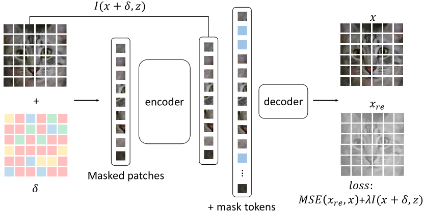
Figure 1: The structure of MIMIR. First, we generate adversarial perturbation $\delta$ and apply it to the input image. Then, following the original ViT, we use separated image patches as input for the autoencoder. We use the decoder output, i.e., $x_{re}$, and the clean input image, i.e., $x$, to calculate the loss. Finally, we use MI ($I(x+\delta,z)$) as an additional penalty in the pre-training loss. After pre-training, the encoder plus a classification layer is fine-tuned for classification tasks.

2 Background

2.1 Adversarial Attack

An adversarial attack [23, 11, 71] refers to applying imperceptible perturbations to the original input of the target machine learning model (in this work, neural network), which generates adversarial examples to fool the victim model. Given an $L$-layer neural network $F_{\theta}$ for classification in $d_{Y}$-dimensional space, and a training dataset $D=\{\setargs{(x_{i},y_{i})}\}_{i=1}^{n}$ in $d_{X}$-dimensional space, the two primary goals of adversarial attacks are:

1. The generated perturbation $\delta$ can successfully mislead the network by maximizing (e.g., PGD attack [55]):

   $$\mathop{\max}\limits_{\delta\in S}\mathcal{L}_{CE}(\theta,x_{i}+\delta,y_{i}),$$ (1)

   where $x_{i}\in\mathbb{R}^{d_{X}}$ and $y_{i}\in\{\setargs{0,1}\}^{d_{Y}}$, $\theta$ are the parameters of the current network and $\mathcal{L}_{CE}$ is the standard CE loss. The perturbation aims to decrease confidence in the ground truth labels while increasing confidence in wrong labels. Thus, the loss between the misleading outputs and the ground truth labels increases.

2. The generated adversarial examples are as similar as possible to the original clean examples by limiting $\delta$ to a relatively small domain:

   $$S=B(x_{i},r)=\{\setargs{\delta\in\mathbb{R}^{d_{X}}:\left\|\delta\right\|_{\infty}\leq r}\},$$ (2)

   where $S$ is the $l_{\infty}$-ball of radius $r$ at a position $x_{i}$ in $\mathbb{R}^{d_{X}}$. The distance between $x_{i}$ and $x_{i}+\delta$ can be evaluated by norms such as $l_{0},l_{2},$ and $l_{\infty}$.

When using the above attacks to generate adversarial examples for training, the learning objective is:

$$\mathop{\min}\limits_{\theta}\mathop{\max}\limits_{\delta\in S}\mathcal{L}_{CE}(\theta,x_{i}+\delta,y_{i}).$$ (3)

2.2 Masked Image Modeling - MIM

MIM refers to a self-supervised pre-training framework that aims to reconstruct pre-defined targets, such as discrete tokens [7], raw RGB pixels [36, 49], or features [85]. The final goal is to use the pre-trained model as a starting point for downstream fine-tuning. The downstream tasks include, for instance, classification and object detection. More specifically, to build a high-performance ViT $f_{e}$ without a classification layer, we consider $f_{e}$ as an encoder to extract discriminative input features. Then, we design a lightweight decoder $f_{d}$, which uses the output of $f_{e}$ as its input. The goal of $f_{d}$ is to reconstruct the original inputs (let us consider MAE [36] as an example). The aim is to decrease the distance between the input $x$ and $x_{re}=f_{d}\circ f_{e}(x)$. After the encoder $f_{e}$ and decoder $f_{d}$ are trained, we use $f_{e}$ plus a manually initialized classification layer as the starting point of fine-tuning.

2.3 Mutual Information - MI

MI measures the mutual dependence between two random variables, $X$ and $Y$. It quantifies the amount of information contained in one random variable about another random variable or the reduced uncertainty of a random variable when another random variable is known. It can be written as:

$$I(X,Y)=\int_{\mathcal{Y}}\int_{\mathcal{X}}P_{(X,Y)}(x,y)\log\left(\frac{P_{(X,Y)}(x,y)}{P_{(X)}(x)P_{(Y)}(y)}\right),$$ (4)

where $P_{(X,Y)}$ is the joint probability density function of $X$ and $Y$. $P_{(X)}$ and $P_{(Y)}$ are the marginal probability density function of $X$ and $Y$. In addition, MI can be equivalently expressed as:

$$I(X,Y) =H(X)-H(X|Y).$$ (5)

However, quantifying MI is difficult in practice, as it is difficult to precisely estimate $P_{X,Y}$ or $P_{X}$ and $P_{Y}$ in high dimensional space [31]. DIB [94] suggested using the matrix-based Renyi’s $\alpha$-order entropy $I_{\alpha}$ [66, 93] to estimate MI, which avoids density estimation and variational approximation. An alternative way is the Hilbert-Schmidt Independence Criterion (HSIC) [34], which is a kernel-based dependence measure defined in a reproducing kernel Hilbert space (RKHS) and usually used as a surrogate of MI. Details about definitions and empirical estimators of $I_{\alpha}$ and HSIC are provided in Appendix G. In this paper, we use both $I_{\alpha}$ and HSIC as our MI measurements.

2.4 Information Bottleneck - IB

The IB concepts were first proposed in [72] and further developed for deep learning in [73, 68]. It has been widely used to improve adversarial robustness [90, 2, 94, 84]. IB describes the generalization of a deep network in two phases: 1) empirical error minimization (ERM) and 2) representation compression [68]. For a network with input $x$ and label $y$, there is an intermediate representation $t_{l}$ for each layer $l$, i.e., the output of $l$-th layer. The IB principle aims to keep more relevant information in $t_{l}$ about target $y$ while decreasing the irrelevant information about input $x$. The information between intermediate representation $t_{l}$ and input $x$ or label $y$ is quantified by MI, denoted by $I(\cdot)$. During neural network training, in the ERM phase, the model increases shared information between $t_{l}$ with respect to both $x$ and $y$. Afterward, in the compression phase, the model decreases information contained in $t_{l}$ about $x$ but preserves (or even increases) information about $y$. The reduction of $I(x,t_{l})$ can be interpreted as a way of reducing noise or compressing irrelevant or redundant features in $x$. At the end of the training, the model strikes a trade-off that maximizes $I(y,t_{l})$ and minimizes $I(x,t_{l})$. Formally, the IB minimizes the following Lagrangian:

$$\mathcal{L}=I(x,t_{l})-\beta I(y,t_{l}),$$ (6)

where $\beta$ is a Lagrange multiplier that controls the trade-off between predicting $y$ and compressing $x$.

3 MIMIR

3.1 Threat Model

We assume the adversary intends to create adversarial examples from clean images. The adversary has the strongest ability, i.e., the white box, to access the target model. Then, adversarial examples can be created according to model architectures, parameters, the gradients of loss function, and datasets. In addition, the adversary is also aware of potential defenses. An adversary can design new attacks for a specific model according to the details of our defense method.

From the defender’s perspective, the main goal is to train a robust model against potential adversarial attacks. The defender considers the following four objectives:

• The performance on clean data should not decrease significantly. We allow a small drop of clean accuracy for a trade-off in robustness.

• The accuracy of models trained by MIMIR should be significantly higher than for models without defenses under various adversarial attacks.

• Deploying MIMIR should be efficient and scalable to large datasets such as ImageNet-1K [26].

• MIMIR should be robust against adaptive attacks.

3.2 Design Intuition

MIM has been proved useful as a pre-training method for ViTs on various tasks [79, 36, 85, 7]. To train a powerful model by MIM, one can mask out a part of the foreground of inputs and reconstruct it using the model. Masking out the foreground instead of the background reduces discriminative information in visible information to the model. Reconstructing foreground parts is harder than background and helps the model learn more discriminative information [81]. Inspired by this phenomenon, we aim to build a more difficult task by adding adversarial perturbation to clean inputs. The adversarial perturbation increases the distance between the input and reconstruction target. If we can reconstruct clean inputs from adversarial examples, it means the features learned by the model are robust against adversarial attacks. In other words, we want the encoder to learn a latent representation that does not carry information concerning adversarial inputs while enabling the decoder to reconstruct the clean image. Note that simply masking out all foreground does not make sense, as it would not be possible to reconstruct meaningful content. From the perspective of IB, there is a bottleneck between the encoder and decoder. Our adversarial pre-training task contains two information sources: the clean data $x$ and the adversarial perturbation $\delta$. As the information flows through the bottleneck, adversarial information from $\delta$ is eliminated. The natural information from $x$ is maintained because of the constraint when reconstructing the target $x$.

3.3 Design Details

Autoencoder. MIMIR follows the general design of MAE [36], which consists of an encoder $f_{e}$ and a decoder $f_{d}$. Like all other autoencoders, the encoder extracts discriminative features $z$ from inputs $x$. The decoder reconstructs original inputs according to the discriminative features. Following ViT [28], the input $x$ is separated into non-overlapping image patches. Then, we randomly mask out a part of the patches and use the remaining patches as inputs for the following process in the encoder. This random masking process uses uniform distribution to prevent potential sampling bias, such as all foreground information being masked, as it is not possible to find the reconstruction target then. Therefore, we hope to keep a part of the foreground as a hint for reconstruction. The information of masked content is recorded as mask tokens $m$, which are not used by the encoder but will be used later by the decoder. Each token is a learned vector that indicates the presence of a masked patch to be predicted. The mask token is shared by all inputs of the decoder. Like unmasked patches, mask tokens are also assigned corresponding positional embeddings to be in the correct location in the reconstructed image. We emphasize that mask tokens are not used in the encoder part.

To train a ViT, we use the same transformer blocks as ViT to build the encoder. The encoder only processes the visible patches, making training much more efficient. When converting to other architectures, such as ConVit [24], we use corresponding transformer blocks to build the encoder. The decoder accepts the encoded visible image patches and mask tokens as inputs. The decoder is built using the same transformer blocks as the encoder instead of using ViT [28] transformer blocks for all. Then, the decoder is followed by a fully connected layer, which outputs the same number of patches as the original image.

Adversarial pre-training target. The training target is to extract discriminative features from visible image patches by the encoder and then reconstruct the invisible patches by the decoder. Therefore, we need a differentiable measurement to quantify the distance between the original image and the reconstructed results. Following the original MAE [36], this distance is measured by Mean Squared Error (MSE). To create a more difficult reconstruction task, we apply adversarial perturbation $\delta$ on the inputs of the encoder. Thus, the adversarial perturbation is also masked along with the image when inputted into the encoder. The decoder reconstructs the original clean inputs by using the latent features $z$ extracted from adversarial examples. The outputs of decoder $x_{re}$ and $x$ are used to calculate the MSE loss, which is further used to optimize the model. Note that the reconstruction differs from the original MAE; we do not use the encoder inputs as reconstruction targets. Formally, the pre-training process (described in Algorithm 1) can be written as follows:

$$z =f_{e}(x+\delta),$$ (7)

$$x_{re}=f_{d}(z),$$

$$loss_{\text{mse}} =\mathcal{L}_{\text{mse}}(x,x_{re}).$$

MI as penalty. Inspired by IB, we show in Section 3.4 that MI between latent representation and adversarial examples decreases with respect to the accuracy on adversarial example, i.e., $I(x+\delta,z)$ is decreasing while training. Motivated by this finding, we directly use $I(x+\delta,z)$ as a penalty in our final loss function:

$$loss_{\text{mi}} =\mathcal{L}_{\text{mse}}(x,x_{re})+\lambda I(x+\delta,z),$$ (8)

where $\lambda$ is a regularizer for the MI penalty. We use $I(x+\delta,z)$ instead of $I(x,z)$ as a penalty. This is because $x\to x+\delta\to z$ follows the Markov chain since $z$ is extracted from $x+\delta$. According to Data Processing Inequality (DPI) [8], $I(x,z)\leq I(x+\delta,z)$. Minimizing $I(x,z)$ in loss equals minimizing a lower bound of $I(x+\delta,z)$.

Algorithm 1 Masked Adversarial Pre-Training

0:  training data $D$, number of epochs $E$, encoder $f_{e}$, decoder $f_{d}$, network parameters $\theta$, $\mathcal{L}_{\text{mse}}$, $\lambda$.

0:  optimized weights $\theta$

1:  for $e=0\to E-1$ do

2:     $x\leftarrow$ sample_batch($D$)

3:     $\delta\leftarrow$ random_initialization

4:     $x_{re}\leftarrow f_{d}\circ f_{e}(x+\delta)$

5:     $\delta\leftarrow\mathop{max}\limits_{\delta\in S}\mathcal{L}_{\text{mse}}(x+\delta,x_{re})$

6:     Forward:

7:     $z\leftarrow f_{e}(x+\delta)$

8:     $x_{re}\leftarrow f_{d}(z)$

9:     $loss\leftarrow\mathcal{L}_{\text{mse}}(x,x_{re})+\lambda I(x+\delta,z)$

10:     Backward:

11:     $\theta\leftarrow\theta-\alpha\nabla loss$

12:  end for

Generating adversarial examples. To conduct the adversarial pre-training, we need an attack that finds proper adversarial perturbation $\delta$. As the autoencoder does not provide classification outputs, it is not possible to directly use existing adversarial attacks, such as PGD [55]. Still, we can easily design a new algorithm to find $\delta$ by maximizing $loss_{\text{mse}}$ in Eq. (7). As the feature $z$ is extracted from only visible image patches, we only attack the visible patches. We do not add any perturbation to mask tokens since the outputs of the autoencoder are only impacted by visible patches. Then, the adversarial pre-training learning objective can be written as:

$$\begin{split}\mathcal{L}_{\text{adv}}=\mathop{\max}\limits_{\delta\in S}&\mathcal{L}_{\text{mse}}(f_{d}\circ f_{e}(x+\delta),x),\\ \mathop{\min}\limits_{\theta}\mathcal{L}_{\text{adv}}&+\lambda I(x+\delta,z),\end{split}$$ (9)

where $\theta$ are the parameters of the autoencoder.

Adversarial fine-tuning. After the autoencoder is trained, we discard the decoder and initialize a classification layer for the encoder to build a complete model. We use simple adversarial training, PGD [55], to fine-tune our pre-trained models so that we can ensure the improvements come from the MIMIR pre-training. The complete model is trained at the fine-tuning stage.

3.4 Theoretical Justification

In this section, we provide theoretical justification showing that the MI between the adversarial example and its latent representation, i.e., $I(x+\delta,z)$, should be constrained. Let $F$ be any classifier trained on clean samples with desirable prediction accuracy, which may suffer from adversarial attacks. We begin our analysis by first presenting Lemma 3.1.

Lemma 3.1

Given an arbitrary classifier $F$, let $F(x+\delta)$ and $F(x_{re})$ denote, respectively, the predicted labels of adversarial sample $x+\delta$ and reconstructed sample $x_{re}$. We have:

$$I(F(x+\delta),F(x_{re}))\leq I(F(x+\delta),x_{re})\leq I(x+\delta,z).$$ (10)

Proof:

There are two Markov chains:

$$x+\delta\rightarrow F(x+\delta),$$ (11)

$$z\rightarrow x_{re}\rightarrow F(x_{re}),$$

which indicate that $F(x+\delta)$ is an indirect observation of $x+\delta$, whereas both $F(x_{re})$ and $x_{re}$ are indirect observations of $z$.

By the data processing inequality (DPI), we have

$$I(x+\delta,z)\geq I(F(x+\delta),z),$$ (12)

and

$$I(F(x+\delta),z)\geq I(F(x+\delta),x_{re})\geq I(F(x+\delta),F(x_{re})).$$ (13)

∎

Now, we define $p_{e}$ as the probability that the predicted label of $x+\delta$ by $F$ is not equal to that of $x_{re}$, i.e., $p_{e}=\mathbb{P}(F(x+\delta)\neq F(x_{re}))$. Intuitively, our autoencoder is trained to only recover clean sample $x$ without any interference from $\delta$. Hence, a relatively large value of $p_{e}$ is expected. In the following, we establish the connection between $p_{e}$ and $I(x+\delta,z)$ with both lower and upper bounds, showing that minimizing $I(x+\delta,z)$ also encourages a large value of $p_{e}$.

Proposition 3.2

Let $H(\cdot)$ denote the information entropy and $H_{b}(p_{e})=-p_{e}\log_{2}p_{e}-(1-p_{e})\log_{2}(1-p_{e})$ be the binary entropy, we have:

$$H(F(x+\delta))-H_{b}(p_{e})-p_{e}\log(|F(x+\delta)|-1)\leq I(x+\delta,z),$$ (14)

where $|F(x+\delta)|$ is the total number of categories.

Proof:

By the chain rule of MI, we have

$$I(F(x+\delta),F(x_{re}))=H(F(x+\delta))-H(F(x+\delta)|F(x_{re})).$$ (15)

By applying Fano’s inequality [30, 58], we obtain:

$$H(F(x+\delta)|F(x_{re}))\leq H_{b}(p_{e})+p_{e}\log(|F(x+\delta)|-1).$$ (16)

Adding $I(F(x+\delta),F(x_{re}))$ to both sides of Eq. (16):

$$H(F(x+\delta)) -H_{b}(p_{e})-p_{e}\log(|F(x+\delta)|-1)$$ (17)

$$\leq I(F(x+\delta),F(x_{re}))$$

$$\leq I(x+\delta,z).$$

The last line of Eq. (17) is by Lemma 3.1. ∎

Therefore, we obtain a lower bound of $I(x+\delta,z)$. If we use CIFAR-10 ($|F(x+\delta)|=10$) and assume the predicted labels $F(x+\delta)$ follow a uniform distribution, we can visualize the lower bound as a function of $p_{e}$ as shown in Figure 2, from which we observe an obvious monotonic inverse relationship between $I(x+\delta)$ and $p_{e}$ in the range $p_{e}\in[0,0.9]$.

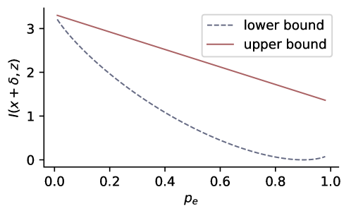
Figure 2: The example plots for the lower and upper bounds on the MI in Propositions 3.2 and 3.3. The entropy ($H(\cdot)$) is chosen uniformly at random from a set of 10 classes. The lower bound reaches its minimum at $p_{e}=0.9$.

In fact, we can also obtain an upper bound, under the assumption that $I(F(x+\delta),x_{re})\approx I(x+\delta,z)$, i.e., there is no information loss in the two Markov chains in Eq. (11).

Proposition 3.3

If $I(F(x+\delta),x_{re})\approx I(x+\delta,z)$, we have:

$$I(x+\delta,z)\lesssim H(F(x_{re}))-2p_{e},$$ (18)

in which the notation “$\lesssim$” refers to less than or similar to.

Proof:

By the Hellman-Raviv inequality [38, 13], we have:

$$2p_{e} \leq H(F(x+\delta)|x_{re})$$ (19)

$$=H(F(x+\delta))-I(F(x+\delta),x_{re})$$

$$\approx H(F(x+\delta))-I(x+\delta,z).$$

∎

Similar to the lower bound, the upper bound also indicates $I(x+\delta,z)$ is inversely proportional to $p_{e}$ as shown in Figure 2.

In fact, apart from the above-mentioned lower and upper bounds, there exists an alternative and intuitive way to understand the mechanism of minimizing $I(x+\delta,z)$. For simplicity, let us assume the clean data $x$ and adversarial perturbation $\delta$ are independent, then:

$$I(x+\delta,z)=I(x,z)+I(\delta,z).$$ (20)

According to [78], minimizing the expected reconstruction error between clean sample $x$ and corrupted input $x+\delta$ amounts to maximizing a lower bound of the mutual information $I(x,z)$, even though $z$ is a function of the corrupted input. Therefore, by minimizing $I(x+\delta,z)$, the network is forced to minimize $I(\delta,z)$ (since $I(x,z)$ is maximized). In other words, only the information about $\delta$ has been removed from $z$. This also explains the robustness of $z$.

TABLE I: Different learning rates. Fine-tuned for 50 epochs.

Dataset	Models	LR	Natural	PGD10
CIFAR-10	ViT-T	5.0e-4	76.30	47.60
		1.0e-3	80.69	49.56
		1.0e-2	85.62	48.78
		5.0e-2	85.12	50.30
		1.0e-1	84.51	50.40

TABLE II: Top 1 natural and adversarial accuracy on CIFAR-10 test set. The results of ARD+PRM [57] are taken from the original paper. As there is no ViT-T architecture, we use the same architecture as DeiT-T.

Dataset	Models	Pre-train	Fine-tune	Natural	PGD20	PGD100	AA
CIFAR-10 [46] ($l_{\infty},\epsilon=8/255$)	ViT-T (DeiT-T)	ImageNet-1K	PGD	75.46	48.10	47.96	43.62
		MAE [36]	PGD	79.89	48.64	48.43	44.27
		ImageNet-1K	ARD+PRM [57]	79.60	50.33	50.15	45.99
		MIMIR	PGD	84.82	57.51	57.38	52.96
	ViT-S	ImageNet-1K	PGD	79.59	50.86	50.73	46.37
		MAE [36]	PGD	85.97	54.19	53.94	50.49
		ImageNet-1K	ARD+PRM [57]	81.86	51.73	51.46	47.33
		MIMIR	PGD	88.11	56.63	56.34	53.18
	ViT-B	ImageNet-1K	PGD	83.16	52.98	52.71	49.06
		MAE [36]	PGD	88.86	57.03	56.86	52.42
		ImageNet-1K	ARD+PRM [57]	84.90	53.80	53.51	50.03
		MIMIR	PGD	89.30	58.07	57.87	54.55
	ConViT-T	ImageNet-1K	PGD	53.09	33.63	33.61	29.65
		MAE [36]	PGD	75.49	45.29	45.17	41.12
		ImageNet-1K	ARD+PRM [57]	80.28	49.86	49.55	45.42
		MIMIR	PGD	80.74	49.37	49.16	45.04
	ConViT-S	ImageNet-1K	PGD	54.03	34.61	34.60	30.60
		MAE [36]	PGD	86.43	54.76	54.59	51.13
		ImageNet-1K	ARD+PRM [57]	84.32	53.10	52.81	48.85
		MIMIR	PGD	87.49	56.35	56.20	52.54
	ConViT-B	ImageNet-1K	PGD	61.54	38.77	38.71	34.21
		MAE [36]	PGD	89.03	58.19	57.75	54.25
		ImageNet-1K	ARD+PRM [57]	85.80	53.36	53.05	49.33
		MIMIR	PGD	89.30	59.31	59.01	55.64

4 Experimental Evaluation

4.1 Experimental Setup

We use PyTorch [60] 2.1.0 for implementation, and mixed precision [56] to accelerate training. We use three datasets to comprehensively evaluate MIMIR: CIFAR-10 [46], Tiny-ImageNet [47], and ImageNet-1K [26], details of datasets are given in Appendix A. Appendix B provides details about decoder hyperparameters.

Model Architecture: We evaluate MIMIR with three commonly used architectures with multiple scales: ViT [28], ConViT [24], and XCiT [3].

Hardware. Experiments are performed on a single machine with 4 RTX A6000 (48GB) and 4 RTX A5000 (24GB) GPUs, CUDA 12.0.

Training hyperparameters. For all experiments, we train models from scratch (unless otherwise specified). Following MAE [36], we do pre-training by MIMIR for 800 epochs and then fine-tuning for 100 epochs. The number of warmup epochs is 40 and 10 for pre-training and fine-tuning, respectively. We use AdamW [53] as an optimizer for both pre-training and fine-tuning. We use cosine decay as the learning rate scheduler.

At pre-training, one-step FGSM with random initialization achieves better performance than using ten-step PGD in Table VII. Therefore, we use a one-step algorithm to generate adversarial examples for all three datasets. The perturbation budget is $\epsilon=8,\alpha=10$. At fine-tuning stage, we use a 10-step PGD algorithm to generate adversarial examples for training to be aligned with baselines. The perturbation limit is $\epsilon=8,\alpha=2$. When fine-tuning with ImageNet-1K, we use one-step FGSM with random initialization to align with baselines and for better efficiency. Following previous research [86, 87], we fine-tuned twice for two different perturbation limits, $\epsilon=2,\epsilon=4$.

As discussed in Section 4.3, strong data augmentation is harmful to adversarial training at a common training schedule (50 or 100 epochs for fine-tuning). We only use simple augmentations, including random resized crops and random horizontal flips.

Previous research used rather different fine-tuning learning rates, so we chose the learning rate by testing different values as given in Table I. We use the best, i.e., $5.0e-2$, as the base learning rate (blr) for CIFAR-10. The learning rate is calculated based on blr, i.e., $lr=blr\times\frac{batchsize}{256}$. For Tiny-ImageNet and ImageNet-1K, we use the same blr as MAE [36], i.e., $0.001$. At the pre-training stage, we use $1.5e-4$ as the learning rate for all datasets. In addition, we noticed that it is possible to get NaN (Not a Number) for loss in a few cases while adversarial training, i.e., the training fails. We solve this problem by using a learning rate that is ten times smaller. More details about hyperparameters can be found in the Appendix D.

TABLE III: Top 1 natural and adversarial accuracy on ImageNet-1K.

Dataset	Models	Pre-train	Fine-tune	$\epsilon=2/255$			$\epsilon=4/255$
				Natural	PGD20	PGD100	Natural	PGD20	PGD100
ImageNet-1K [26] ($l_{\infty}$)	ViT-S	-	FastAT [86]	71.37	49.49	49.41	66.92	34.07	33.82
		-	AGAT [87]	70.62	49.00	48.85	66.10	33.62	33.40
		MIMIR	FastAT [86]	74.60	54.56	54.55	71.29	40.98	40.63
	ViT-B	-	FastAT [86]	70.31	50.55	50.06	65.18	33.59	33.39
		-	AGAT [87]	70.41	51.23	51.11	67.93	34.94	34.78
		MIMIR	FastAT [86]	75.88	55.42	55.36	73.22	41.26	40.46
	CaiT-XXS24	-	FastAT [86]	72.84	54.31	54.26	68.77	32.14	32.09
		-	AGAT [87]	71.15	54.17	54.08	68.22	31.46	31.39
		MIMIR	FastAT [86]	73.39	53.39	53.37	69.90	40.53	40.22
	CaiT-S36	-	FastAT [86]	72.51	53.12	52.76	71.20	33.02	32.84
		-	AGAT [87]	72.69	53.66	53.48	71.06	33.46	33.17
		MIMIR	FastAT [86]	76.05	56.78	56.75	73.57	40.03	39.16

TABLE IV: Comparison of different architectures under 100-step PGD attack.

Dataset	Models	$\epsilon=2/255$		$\epsilon=4/255$
		Natural	PGD	Natural	PGD
ImageNet-1K ($l_{\infty}$)	ViT-S	74.60	54.56	71.29	40.63
	ConViT-S	74.72	55.65	72.08	42.62
	XCiT-S	74.39	55.21	71.77	40.97
	XCiT-M	73.63	53.04	72.01	42.39

TABLE V: The experimental results for natural accuracy of clean images and adversarial accuracy under AutoAttack on Tiny-ImageNet. ${\dagger}$ Note that Wang et at. [83] and Gowal et al. [33] utilize generated data based on ImageNet-1K as augmentation. This is achieved by directly generating images using ImageNet-1K images and the labels of Tiny-ImageNet.

Dataset	Architecture	Method	Generated	Batch	Epoch	Natural	PGD20	PGD100	AA
Tiny-ImageNet [47] ($l_{\infty},\epsilon=8/255$)	WRN-28-10	Gowal et al. [33]	$\times$	512	400	51.56	N/A	N/A	21.56
	WRN-28-10	Wang et at. [83]	1m	512	400	53.62	N/A	N/A	23.40
	WRN-28-10	Gowal et al. [33]${\dagger}$	1m (ImageNet-1K DDPM)	512	800	60.95	N/A	N/A	26.66
	WRN-28-10	Wang et at. [83]${\dagger}$	1m (ImageNet-1K EDM)	512	400	65.19	N/A	N/A	31.30
	ViT-S	MIMIR	1m	512/256	800/100	63.33	26.37	26.17	22.52
	ViT-B	MIMIR	1m	512/256	800/100	65.06	25.41	25.03	22.82
	ConViT-T	MIMIR	1m	512/256	800/100	52.61	24.61	24.58	19.42
	ConViT-S	MIMIR	1m	512/256	800/100	62.29	26.39	26.30	22.88

Evaluation metrics. We use natural accuracy and adversarial accuracy as evaluation metrics. Natural accuracy refers to the accuracy of a model on clean and unmodified inputs. The adversarial accuracy measures the accuracy of a model under a specific adversarial attack. To show that the improvement is not from obfuscated gradient [5], we use PGD [55] and AutoAttack [20] to evaluate the robustness of trained models. PGD is one of the most popular adversarial attacks used for generating adversarial examples. We evaluate MIMIR under 20 and 100 steps of PGD attack. AutoAttack is an ensemble of diverse parameter-free attacks, including white-box and black-box attacks. In our experiments, we use standard version of AutoAttack that contains four attacks, including APGD-ce [20], APGD-t [20], FAB-t [19], and Square [4].

We use the same perturbation budget for our experiments to compare with previous works. We apply the commonly-used $l_{\infty}$ norm for PGD [55] and AutoAttack (AA) [20]. We set the perturbation radius $\epsilon$ to $8/255$ for CIFAR-10 [46] and Tiny-ImageNet [47]. The step length is $\alpha=2/255$. As the image size of ImageNet-1K is much larger, we use different scales of $\epsilon$ for adversarial training and evaluation [26]. Following previous works [57, 87, 50], we use two perturbation radius $2/255,4/255$ for evaluation. The step length is $\alpha=1/255$.

4.2 Experimental Results

Overall performance. We apply MIMIR to CIFAR-10 [46], Tiny-ImageNet [47], and ImageNet-1K [26]. The results are shown in Tables II, III, and V, respectively. Overall, MIMIR significantly improves adversarial accuracy under PGD and AA attacks. While training with CIFAR-10 on ViTs (ViT-S and ViT-B), MIMIR improves the accuracy by an average of 5.50% compared to the baseline. On ConViTs (ConViT-T, ConViT-S, and ConViT-B), MIMIR improves the accuracy by an average of 2.87% compared to the baseline. While using ImageNet-1K on ViTs (ViT-S and ViT-B), MIMIR improves the accuracy by an average of 5.52% compared to the baseline. When fine-tuning with clean data, MIMIR also shows improved natural accuracy in Table XIV. In addition, we also evaluate the time consumption and memory usage of MIMIR in Table X. We compare MIMIR with FastAT [86] and 10-step PGD adversarial training. The results show that using MIMIR for pre-training is much more efficient than traditional adversarial training.

Standard deviation. Due to the high computation cost of training, we cannot report standard deviation for all experiments. To show that our method MIMIR has low variances, we train ViT-S on CIFAR-10 three times with different random seeds, running pre-training 400 epochs and fine-tuning 50 epochs. The natural accuracy is 86.07 $\pm$ 0.16 %. The adversarial accuracy under PGD₂₀ ($l_{\infty},\epsilon=8/255$) is 47.24 $\pm$ 0.12 %.

Comparison with related work. We present the performances of MIMIR compared with recent baseline methods in Tables II and III. In Table II, we perform experiments using CIFAR-10 [46]. The results are compared with three baselines, including pre-training on ImageNet-1K and fine-tuning with PGD, MAE [36], and ARD+PRM [57]. The “ImageNet-1K” under the Pre-train column refers to using models pre-trained on ImageNet-1K, then fine-tuned with PGD for 40 epochs, which is the first baseline in ARD+PRM [57]. The MAE [36] baseline is pre-trained using clean CIFAR-10 images and fine-tuned with 10-step PGD adversarial training. The training schedule of MAE [36] baseline is 800 epochs for pre-training and 100 epochs for fine-tuning. Our MIMIR uses the same training schedule as MAE [36]. We provide results on fine-tuning with clean images in Appendix E. The ARD+PRM [57] baseline refers to the best algorithm in [57], where we use the results from that work. Note that ARD+PRM [57] baseline uses models pre-trained on ImageNet-1K. Using models pre-trained on ImageNet-1K and then fine-tuning for CIFAR-10 can easily get accuracy higher than 95% [75].

As MIMIR only uses CIFAR-10 for training, it is more challenging to achieve good performance. For a more fair comparison, we use elucidating diffusion model (EDM) data as a data augmentation since the baselines also use EDM data (Wang et at. [83] and Rebuffi et al. [62]) or models pre-trained on ImageNet-1K (ARD+PRM [57]). Generative data is usually used to improve adversarial training [83, 61, 63, 33]. Specifically, we use 5 million generated CIFAR-10 data and 1 million Tiny-ImageNet data provided by [83]. Note that the EDM data is generated only based on CIFAR-10 or Tiny-ImageNet, and the MAE baseline uses EDM data as well. The EDM data is applied to experiments with CIFAR-10 and Tiny-ImageNet but not to ImageNet-1K.

According to results in Table II, MIMIR consistently improves adversarial robustness compared to all baselines. It also improves the natural accuracy compared to the MAE baseline. This is because self-supervised MIMIR does not suffer from inconsistency between the ground truth and adversarial example [59]. Let us consider a joint data distribution $p_{d}(x,y)$ (training data) and a discriminative model $p_{\theta}(y|x)$, where $x$ is the data with its label $y$. In standard training, we hope the model learns discriminative features by minimizing the distance between $p_{d}(y|x)$ and $p_{\theta}(y|x)$. In adversarial training, we hope the model is robust by minimizing the distance between $p_{d}(y|x)$ and $p_{\theta}(y|x+\delta)$, i.e., Eq. (3). This means $p_{\theta}(y|x+\delta)$, instead of $p_{\theta}(y|x)$, is encouraged to converge to $p_{d}(y|x)$. Supervised adversarial training builds a shortcut from $x+\delta$ to $y$. For the optimal $\theta^{*}$ of minimizing Eq. (3), $p_{\theta^{*}}(y|x)\neq p_{d}(y|x)$ [59]. Therefore, there is always a trade-off between natural and adversarial accuracy in supervised adversarial training. However, such inconsistency does not apply to self-supervised MIMIR, as there is no label for self-supervised training. MIMIR encourages $p_{\theta_{ae}}(x_{re}|x+\delta)$ to converge to $p_{d}(x)$, which does no affect convergence of $p_{\theta_{ae}}(x_{re}|x)$ to converge to $p_{d}(x)$. This implies that supervised pre-training is harmful to natural accuracy, which is also aligned with the findings of previous research [39].

Table III shows the results evaluated on the ImageNet-1K [26] dataset. The performance of MIMIR is compared with two baselines, including FastAT [86] and AGAT [87]. The FastAT [86] is designed for efficient adversarial training so that it can be applied to large models and large datasets, such as ImageNet-1K. The main idea of FastAT is to use a single-step adversarial attack to generate adversarial examples. The authors refined the standard FGSM [32] by applying a random start at the beginning of the algorithm and a much larger step size to reach the perturbation limit. According to empirical results, they used $\alpha=1.25\times\epsilon$ for step size, which provided comparable performance to the best-reported result from free adversarial training [25]. The results of FastAT [86] and AGAT [87] are taken from [87]. The baselines of FastAT [86] and AGAT [87] are trained for 300 epochs with a cosine decay learning rate schedule, and the first 20 epochs for learning rate warmup. As shown in Table III, the accuracy of AGAT [87] may decrease compared to FastAT [86]. This is because AGAT [87] discards low-attention image patches for efficiency. The image patches, even with the low-attention scores, are useful for classification. In Table IV, we compare the performance among three architectures with multiple scales. MIMIR shows similar performance on other architectures as on the original ViTs, which means MIMIR is well-generalized to different architectures.

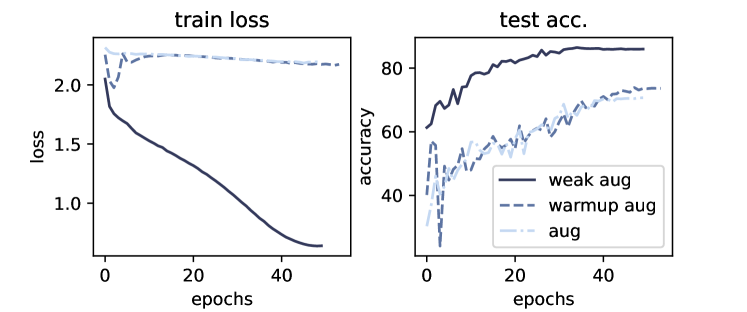
Figure 3: The loss and natural accuracy for three different augmentation strategies, using CIFAR-10 and ViT-small.

As CIFAR-10 is small compared to ImageNet-1K, we also provide experiments on Tiny-ImageNet for completeness. We use the same training schedule and hyperparameters for experiments on Tiny-ImageNet. As AGAT [87] and ARD+PRM [57] do not provide experiments on Tiny-ImageNet, we compare our results with the most recent adversarial robustness results from Wang et at. [83] and Rebuffi et al. [62]. They use generated data as augmentation for more robust adversarial training. Specifically, Gowal et al. [33] study four methods for generated data as augmentation, including Denoising Diffusion Probabilistic Model (DDPM) [41], Very Deep Variational Auto-Encoder (VDVAE) [18], StyleGAN [45], and BigGAN [12]. Wang et at. [83] demonstrated better diffusion models and further improved adversarial robustness compared to previous works. In Table V, we show our experimental results compared with previous works.

Our method provides competitive performance. Especially when the baselines only use generated data based on Tiny-ImageNet, MIMIR provides the best natural accuracy (65.06%). When the baselines use generated data based on ImageNet-1K, and we only use that based on Tiny-ImageNet, MIMIR still shows comparable performance. In addition, according to Table X, the MIMIR training schedule (800 pre-training + 100 fine-tuning) takes approximately 200 fine-tuning (10-step PGD) epochs of training time. Thus, MIMIR costs much less training time and gets comparable results to baselines.

TABLE VI: Data augmentation ablation with longer fine-tuning schedule.

Models	Epoch	Augmentation	Natural	PGD20
ViT-B	800	Weak Augmentation	89.90	60.26
		+ CutMix [95],MixUp [97]	91.01	60.62
		+ Randaugment [21]	90.19	62.75

4.3 Data Augmentation is Harmful

As mentioned in previous works [6, 25], strong data augmentation makes the training samples too difficult to be learned by ViTs while conducting adversarial training. The strong data augmentation refers to the combination of Randaugment [21], CutMix [95], and MixUp [97]. In this section, we evaluate two different solutions to ease this problem. First, we only use simple data augmentation for adversarial training, including random crop (or random resize crop for ImageNet-1K) and random horizontal flip (“weak aug”). Second, we use a 10-epoch warmup procedure for strong data augmentation. The warmup of Randaugment is implemented by progressively increasing the distortion magnitude from 1 to 9 (“warmup aug”). For CutMix and MixUp, we warm up by increasing the mixup probability from 0.5 to 1.0. As shown in Figure 3, “weak aug” provides the best accuracy. The “warmup aug” shows a slightly improved accuracy compared to fusing strong augmentation. Therefore, we provide a different result from [6] on the smaller dataset CIFAR-10, i.e., we show that weak augmentation is better than warmup augmentation. Even data augmentation with reduced amplitude is still difficult to learn at the beginning of adversarial training. Although strong augmentation is harmful to a normal training schedule, we show in Table VI that CutMix [95], MixUp [97], and Randaugment [21] increase the accuracy of adversarial training when training with a longer schedule, e.g., 800 epochs of fine-tuning. We conjecture that the data with strong augmentation is helpful but difficult for adversarial training to learn. Thus, it needs more epochs to learn meaningful representation. Loss and accuracy curves can be found in Appendix C. Due to the longer schedule, we use patch size 4 to reduce training time.

TABLE VII: Comparison between HSIC and $I_{\alpha}$. Models are pre-trained for 800 epochs. For fine-tuning, all models are adversarially trained with 10-step PGD for 50 epochs.

Pre-train	$\lambda$	Estimator	Natural	PGD
MIMIR	0.001	HSIC [34]	69.63	43.17
MIMIR	0.001	$I_{\alpha}$ [94]	75.00	46.11
MIMIR	1e-05	HSIC [34]	76.30	47.60
MIMIR	1e-05	$I_{\alpha}$ [94]	75.53	46.75
MIMIR	1e-06	HSIC [34]	74.90	46.19
MIMIR	1e-06	$I_{\alpha}$ [94]	74.60	45.66
Adv-MAE (1-step)	0.0	-	74.69	46.28
Adv-MAE (10-step)	0.0	-	73.96	45.77
MAE	0.0	-	69.02	42.31

4.4 MI Measures

In Section 3.4, we provide lower and upper bound (Eq. (14)) of $I(x+\delta,z)$. According to the two bounds, $I(x+\delta,z)$ is supposed to decrease while the autoencoder learns to reconstruct the clean image $x$. This motivates us to directly embed $I(x+\delta,z)$ as a minimizing learning objective. Before achieving the goal, we must choose a suitable and efficient MI estimator and a regularizer ($\lambda$ in Eq. (8)). In this paper, we use $I_{\alpha}$ [94] and HSIC [54] as estimators. In Table VII, we show the performance of $I_{\alpha}$ [94] and HSIC [54] with different values of $\lambda$. According to the results, using HSIC as an estimator with $\lambda=1e-05$ shows the best performance, which is used for other experiments.

We also show that MIMIR outperforms original MAE [36] and Adv-MAE [91]. To make it clearer, the MAE baseline in Table VII refers to using the original MAE for pre-training and then fine-tuning with 10-step PGD. Adv-MAE refers to using adversarial examples but not using $I(x+\delta,z)$ in loss. Adv-MAE (10-steps) refers to using the 10-step PGD algorithm ($\epsilon=8,\alpha=2$) to generate adversarial examples at pre-training. Adv-MAE provides better accuracy than MAE, which supports our statement that using adversarial examples in Masked Image Modeling creates a more difficult reconstruction task. This more difficult task further improves the performance of downstream models. We use the default learning rate (i.e., $5.0e-4$) of MAE [36] in experiments in Table VII. This is aligned with Adv-MAE [91].

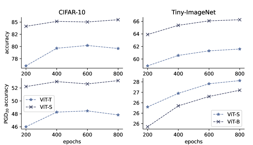
Figure 4: The fine-tuning results with different numbers of pre-train epochs. The left column is trained on CIFAR-10, and the right column is on Tiny-ImageNet. The above is natural accuracy, and the below is adversarial accuracy under a 20-step PGD attack.

4.5 Training Epochs Ablation Study

Our experiments so far are based on 800-epoch pre-training. In Figure 4, we show the influence of different numbers of epochs. We use ViT-T and ViT-S as our baseline models for CIFAR-10, ViT-S, and ViT-B for Tiny-ImageNet. We fine-tune each model 50 epochs after MIMIR pre-training. Both adversarial and natural accuracy are improved with a longer training schedule. On CIFAR-10, the improvement of ViT-T is more significant than that of ViT-S. On Tiny-ImageNet, the increase is more obvious.

4.6 Fine-tuning Using Advanced Methods

Our fine-tuning thus far is based on traditional 10-step PGD adversarial training for CIFAR-10. The reason is to compare with previous works that use a 10-step PGD algorithm. Next, we consider using TRADES [96] and MART [82] to study whether MIMIR can achieve better performance with better fine-tuning methods. TRADES [96] identify a trade-off between robustness and accuracy on clean data. The authors decompose the prediction error of adversarial examples as natural and boundary errors. According to these two kinds of errors, the authors find a differentiable upper bound based on the theory of classification-calibrated loss. MART [82] finds that misclassified and correctly classified natural examples have different influences on the final robustness after adversarial training. Therefore, the authors designed MART to explicitly differentiate the misclassified and correctly classified natural examples during adversarial training.

In Table VIII, the MIMIR performance could be further improved with the two advanced adversarial training methods. Specifically, TRADES slightly improves the accuracy on clean examples but shows worse robustness compared to PGD. MART improves the adversarial accuracy when using ViT-B, but we notice a significant drop in natural accuracy.

TABLE VIII: The experimental results with different fine-tuning methods.

Models	Method	Natural	PGD20	PGD100	AA
ViT-S	PGD	88.11	56.63	56.34	53.18
	TRADES	88.19	56.42	56.36	51.70
	MART	80.55	50.81	50.75	39.92
ViT-B	PGD	89.30	58.07	57.87	54.55
	TRADES	90.91	57.73	57.58	52.79
	MART	85.78	60.35	60.16	54.27

4.7 Adaptive Attack Evaluation

As the adversary is aware of the defense MIMIR, they can design adaptive attacks [76]. For example, the adversary may attack feature space [52, 65] since MIMIR trains backbone to extract features. Here, the backbone refers to the ViT model without the final classification layer, i.e., the encoder of MIMIR. In this section, we provide two adaptive attacks specifically designed against MIMIR. First, we introduce PGD-MI, which utilizes the MI $I(x+\delta,z)$ to generate adversarial examples, as $I(x+\delta,z)$ is used in MIMIR pre-training as a penalty in loss. Therefore, it is reasonable to attack the model by directly increasing the MI $I(x+\delta,z)$. Formally, we embed the following loss into the PGD algorithm:

$$\mathop{\max}\limits_{\delta\in S}\mathcal{L}_{CE}(x_{i}+\delta,y_{i})+\lambda I(x+\delta,z).$$ (21)

We use the same value of $\lambda$ as in MIMIR pre-training.

Second, we introduce PGD-feature that directly attacks the feature extracted by ViT backbones. As the backbones are trained by self-supervised MIMIR pre-training (the whole model is trained when fine-tuning), we hope to evaluate the feature extracted by the backbones. The PGD-feature increases the distance between features extracted from clean and adversarial examples. We implement it using the $L_{2}$ norm and the PGD algorithm:

$$\mathop{\max}\limits_{\delta\in S}l_{2} (f_{e}(x),f_{e}(x+\delta)).$$ (22)

Table IX shows the adaptive evaluation results for PGD-MI and PGD-feature. We use 100 steps for both to make sure the attacking algorithm converges. The perturbation budget is the same as the previous evaluation, i.e., $\epsilon=8/255$. For ImageNet-1K, we use $\epsilon=4/255$. According to the results in Table IX, MIMIR is still robust against adaptive attacks.

4.8 Evaluation of the Loss Surface

To show that the robustness of MIMIR-trained models does not stem from gradient masking, we plot loss surfaces [48] in Figure 5. The loss surface is the visualization of the loss function as parameters change. The basic idea is to plot the loss around the optimal parameters. Formally, we consider in the 2D case:

$$f_{l}(\alpha,\beta)=L(\theta^{*}+\alpha\theta_{1}+\beta\theta_{2}),$$ (23)

where $\theta_{1}$ and $\theta_{2}$ are two direction vectors, $\alpha$ and $\beta$ are two arguments of $f_{l}$. In practice, we use the parameters of trained models, i.e., $\theta^{*}$. In Figure 5, we provide the loss surfaces for models. The surfaces of all models are smooth, i.e., the gradient at a certain point is clear and can also be easily estimated by local average gradients, which means the gradient is masked.

Figure 5: The loss surfaces of the models. The four figures of each column are the loss information of one model. The first column is ConViT-S pre-trained with MIMIR and fine-tuned with adversarial examples. The second column is ConViT-S, pre-trained with clean data and fine-tuned with adversarial examples. The third is ViT-S, pre-trained with clean data and then fine-tuned with adversarial examples. The fourth one is ViT-S, pre-trained with MIMIR and fine-tuned with adversarial examples. The training dataset is CIFAR-10.

TABLE IX: The experimental results for adaptive attacks.

Dataset	Model	PGD20	PGD-MI100	PGD-fea100
CIFAR-10	ConViT-S	56.35	56.16	78.52
	ViT-S	56.63	56.31	78.41
	ViT-B	58.14	57.85	80.49
Tiny-ImageNet	ConViT-S	26.39	26.29	58.50
	ViT-S	26.37	26.18	57.36
	ViT-B	25.41	25.05	58.90
ImageNet-1K	ConViT-S	53.86	53.84	72.10
	ViT-S	54.56	54.55	72.27
	ViT-B	55.41	55.36	73.51

4.9 Efficiency

Table X provides the time consumption and memory usage of MIMIR and adversarial training at fine-tuning. The time consumption and memory usage are evaluated on 4 A6000 GPUs. Compared to 10-step PGD and FAST AT, MIMIR shows much less time consumption. At pre-training, MIMIR shows slightly higher time consumption than MAE, resulting from generating adversarial examples and calculating MI between $x+\delta$ and $z$. Still, as we use a one-step algorithm, generating adversarial examples does not cost too much time. We also consider using 10-step PGD at pre-training, Table VII shows that using a one-step algorithm with larger $\alpha=10$ provides better performance. In addition, pre-training with MIMIR also costs less memory. Note in Table X that the batch size for MIMIR pre-training is much larger than the batch size for adversarial fine-tuning. In Table X, a single epoch of MIMIR costs about $\frac{1}{8}$ time consumption compared to 10-step PGD adversarial training, and about $\frac{1}{2}$ compared to 1-step fast adversarial training [86]. Therefore, MIMIR is more promising concerning training costs when conducting adversarial training.

4.10 Discussion and Limitations

Across our experiments, we have observed the promising performance of MIMIR. This is because we build a different adversarial training paradigm. With MIMIR, the adversarial pre-training can be more efficient and effective. Following the idea of IB, we can intuitively consider a bottleneck between the encoder and decoder. As the reconstruction output is constrained by clean data $x$, the bottleneck will filter out information from adversarial perturbation $\delta$. We provide a theoretical guarantee of this bottleneck in Section 3.4. In Eq. (8), we embed this bottleneck as a learning object to further improve the performance. This improvement also confirms the correctness of our theoretical guarantee in Section 3.4. Table VII shows that our method works better than baseline even without embedding the bottleneck in Eq. (8). With the two information sources of $x$ and $\delta$, the model is trained to learn the robust features from $x$ and forget the information of $\delta$ under the constraint of the reconstruction target.

While MIMIR shows better performance, there are still certain limitations. MIMIR is a pre-training method. An adversarial fine-tuning is necessary to build the final model. Thus, the shortcomings of traditional adversarial training cannot be completely avoided. In our experiments, we utilize the simple PGD algorithm for fine-tuning, but one can further improve MIMIR pre-trained models with more advanced approaches. In addition, MIMIR follows the design of MAE, and we also utilize the characteristic that ViTs are capable of processing variable-length inputs. Therefore, currently, MIMIR cannot handle pyramid-based ViTs and CNNs. While it is not trivial to apply MIMIR to other pyramid-based ViTs and CNNs, this is feasible [89, 49, 81].

TABLE X: The average time consumption of a single epoch on 4 GPUs. The “mem.” refers to GPU memory usage.

			CIFAR-10 [46]		Tiny-ImageNet [47]		ImageNet-1K [26]
Models	#Parames (M)	Method	time[S]	mem.[GB]	time[S]	mem.[GB]	time[S]	mem.[GB]
ViT-S	21.34	PGD10 AT	149.3	2.54$\times$4	306.0	3.99$\times$4	2251.7	12.5$\times$4
		FastAT	43.3	2.54$\times$4	67.7	4.03$\times$4	555.5	10.4$\times$4
		MAE	16.1	3.24$\times$4	33.0	3.27$\times$4	269.6	11.1$\times$4
		MIMIR	18.4	3.12$\times$4	40.0	3.18$\times$4	275.5	11.1$\times$4
ViT-B	85.27	PGD10 AT	361.2	5.39$\times$4	1022.2	8.30$\times$4	5416.7	22.1$\times$4
		FastAT	122.8	5.36$\times$4	180.2	8.34$\times$4	1361.3	19.8$\times$4
		MAE	53.0	5.95$\times$4	106.5	5.95$\times$4	490.9	17.0$\times$4
		MIMIR	59.0	6.08$\times$4	122.0	6.11$\times$4	509.9	17.0$\times$4
ConViT-S	27.05	PGD10 AT	442.5	6.64$\times$4	897.0	12.19$\times$4	6626.5	32.5$\times$4
		FastAT	106.5	5.86$\times$4	183.2	10.62$\times$4	1431.2	26.4$\times$4
		MAE	33.0	10.6$\times$4	67.5	10.61$\times$4	609.7	27.5$\times$4
		MIMIR	45.0	10.4$\times$4	90.0	10.54$\times$4	611.1	28.3$\times$4

5 Related Work

5.1 Vision Transformer

The transformers [77] were first proposed in natural language processing (NLP). With the mechanism of global self-attention, transformers can effectively capture the non-local relationships among all text tokens [27, 14, 22]. The pioneering work, ViT [28], demonstrated that the pure transformer architecture can achieve competitive performance on various tasks. ViT also reveals that transformers lack inductive biases [28]. For example, locality, two-dimensional neighborhood structure, and translation equivariance are inherent to CNNs but not applicable to ViTs [28]. Due to this shortcoming, ViTs usually require large-scale training to get competitive performance, such as pre-training on ImageNet-21K [26] and JFT-300M [70]. To alleviate the ViT need for large datasets, DeiT [74] introduced a teacher-student strategy to distill knowledge from a teacher CNN for a student ViT. In the MIM field, MAE [36] uses a masked autoencoder with a lightweight decoder as a visual representation learner. Its learning objective is to reconstruct the original image by the decoder while using masked images as input to the autoencoder. The advantage is that MAE can randomly discard 75% image patches when pre-training under ImageNet-1K [26], which means more efficient training.

5.2 Adversarial Attacks on ViTs

The concept of adversarial attacks first appeared in [23], which proposed a formal framework and algorithms against the adversarial spam detection domain. Then, the adversarial attacks were popularized by Biggio et al. [11] and Szegedy et al. [71] in image classification. The generation of adversarial examples depends on the model’s gradient or estimated gradient in black box situation [43]. Therefore, adversarial attacks can be easily applied to transformers by using the gradient of attention blocks concerning inputs. This also raises a question: are transformers more robust than CNNs? Benz et al. [9] found that CNNs are less robust than ViTs due to their shift-invariant property. Bhojanapalli et al. [10] found that ResNet models are more robust than transformers at the same model size under FGSM attack, but under PGD [55] attack, transformer models show better robustness. As ViTs process the input image as a sequence of patches, Gu et al. [35] found that ViTs are more robust than CNNs to naturally corrupted patches because the attention mechanism is helpful in ignoring naturally corrupted image patches. The later work [6] revealed that CNNs could be as robust as ViTs against adversarial attacks if CNNs are trained with proper hyperparameters.

5.3 Adversarial Defense

Due to the difference between CNNs and ViTs, there have been some recent efforts to explore new adversarial training approaches for ViTs [57, 25, 87]. Mo et al. [57] presented a new adversarial training strategy based on the following observations: 1) pre-training with natural data can provide better robustness after adversarial fine-tuning, 2) gradient clipping is necessary for adversarial training, and 3) using SGD as the optimizer is better than Adam. Debenedetti et al. [25] also presented an improved training strategy for ViTs by evaluating different combinations of data augmentation policies. They found that weak data augmentation and large weight decay are better than previous canonical training approaches. As adversarial training is time-consuming, AGAT [87] leverages the attention score while training to discard non-critical image patches after every layer. Unlike previous works, we provide a different training paradigm by using MIM for adversarial pre-training. Our method is efficient as we discard 75% image patches while pre-training. Our method is effective as we eliminate the information of adversarial perturbation from two information sources of clean and adversarial inputs. We also provide theoretical proof that the information of adversarial perturbation is eliminated.

5.4 Self-Supervised Adversarial Pre-Training

Self-supervised learning [37, 17, 36, 16] refers to extracting meaningful representation from unlabeled data, which can be used for downstream recognition tasks. Self-supervised methods are beneficial for out-of-distribution detection on difficult, near-distribution outliers [40], which leads to using self-supervised training to improve adversarial robustness [15, 40, 44, 29, 88, 64]. The basic idea is to build a min-max learning object similar to traditional adversarial training in Eq. (3). With the development of self-supervision technologies, more advanced technologies, such as contrastive learning and MAE [36], are applied to adversarial pre-training. For example, Jiang et al. [44] considered using two adversarial samples or combining one adversarial sample and one natural sample to learn consistent representation in contrastive learning. In more recent work, You et al. [92] proposed NIM De³ to denoise adversarial perturbation. However, the motivation of these works relies on complex self-supervised pre-training technologies, making it more difficult to understand the inner mechanisms or provide theoretical results. MIMIR not only provides better performance but also provides intuitive insights with theoretical motivation.

6 Conclusions and Future Work

This paper investigates MIMIR as a pre-training method to improve adversarial robustness for ViTs under various benchmark datasets. MIMIR uses adversarial examples as inputs and clean data as the reconstruction target. In this way, the information from the adversarial perturbation is removed by the bottleneck, but the information from clean data is maintained due to the constraint while reconstructing the target. We also theoretically prove that MI between adversarial inputs and their latent representations, i.e., $I(x+\delta,z)$, should be decreased while training. Our experimental results show that MIMIR significantly improves adversarial robustness compared to recent state-of-the-art methods. In addition, a single epoch of MIMIR pre-training costs only about $\frac{1}{8}$ of training time compared to 10-step PGD adversarial training, and about $\frac{1}{2}$ compared to 1-step fast adversarial training [86] (see Table X). The aforesaid limitations of MIMIR represent a good starting point for future work. For example, we will investigate how to apply MIMIR to CNNs and pyramid-based ViTs and build new self-supervised tasks for adversarial training.

Appendix A Datasets

We use three commonly used datasets to evaluate MIMIR: CIFAR-10 [46], Tiny-ImageNet [47], and ImageNet-1K [26]. CIFAR-10 [46] comprises 50,000 images with size $3\times 32\times 32$ in 10 classes. ImageNet-1K [26] is the most commonly used dataset for the evaluation of ViTs and its variants, which is composed of more than 1.2 million high-resolution images in 1,000 classes. In our experiments, images from ImageNet-1K are resized to $3\times 224\times 224$. For completeness, we also include Tiny-ImageNet [47] as a medium size dataset between CIFAR-10 [46] and ImageNet-1K [26]. Tiny-ImageNet [47] contains 100,000 images with size $3\times 64\times 64$ in 200 classes.

Appendix B Decoder Hyperparameters

We use transformer blocks but fewer layers as the backbone of the decoder. For CIFAR-10, we use the patch size of 2, 4 for Tiny-ImageNet, and 16 for ImageNet-1K. Table XI shows the hyperparameters of decoder architectures. For different ViT architectures, we use the transformer blocks of the respective architectures to build the decoder.

TABLE XI: Model architectures of the encoder and decoder.

Model	Layers	Hidden size	MLP ratio	Heads
ViT-T (encoder)	12	192	4	3
decoder	2	128	4	16

Appendix C Data Augmentation Ablation Study

Figure 6 demonstrates the loss and accuracy while training with different augmentations. “no mix” refers to using only weak augmentation, including RandomResizedCrop and RandomHorizontalFlip. “+mix” refers to using MixUp (0.8) and CutMix (1.0). “+aug” refers to using MixUp (0.8), CutMix (1.0), and Randaugment (rand-m9-mstd0.5-inc1).

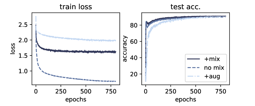
Figure 6: The training results of using different data augmentations with 800 epochs.

Appendix D Details of Training Hyperparameters

In Tables XII and XIII, we provide the default hyperparameters used in our experiments. In addition, we use different patch sizes for different datasets: patch size 2 for CIFAR-10, 4 for Tiny-ImageNet, and 16 for ImageNet-1K. Using smaller patch sizes increases the time consumption when calculating self-attention, but MIMIR pre-training discards 75% patches, making it still efficient. In addition, due to the depth and comparatively small embedding size of CaiT, we use different drop path and layer-wise decay at fine-tuning (for ImageNet-1K). For CaiT-XXS24, we use 0.95 and 0.15 as layer-wise decay and dropout, and 0.85 and 0.35 for CaiT-S36. We also apply stochastic depth decay rule [42] to CaiT. CaiT-S36 models are only fine-tuned 50 epochs due to time-consumption and it is sufficient to get superior results. The batch size to fine-tune CaiT is 512 due to limitation of GPU memory. Other hyperparameters are consistent with Tables XII and XIII.

TABLE XII: Pre-training hyperparameters.

Config	Value
optimizer	AdamW
base learning rate	1.5e-4
weight decay	0.05
optimizer momentum	$\beta_{1}=0.9,\beta_{2}=0.95$
batch size	512(CIFAR-10, Tiny), 2,048 (ImageNet-1K)
learning rate schedule	cosine decay
warmup epochs	40
training epochs	800
augmentation	RandomResizedCrop, RandomHorizontalFlip

TABLE XIII: Fine-tuning hyperparameters.

Config	Value
optimizer	AdamW
base learning rate	0.5e-2 (CIFAR-10), 1e-3 (ImageNet-1K, Tiny)
weight decay	0.05
optimizer momentum	$\beta_{1}=0.9,\beta_{2}=0.999$
layer-wise lr decay	0.65
batch size	128 (CIFAR-10), 256 (Tiny), 1,024 (ImageNet-1K)
learning rate schedule	cosine decay
warmup epochs	10
training epochs	100
augmentation	RandomResizedCrop, RandomHorizontalFlip
drop path	0.1

Appendix E Fine-tuning with Clean Images

In Table XIV, we show the results of MIMIR pre-training with adversarial data, and MAE [36] pre-training with clean data. MIMIR shows comparable and even better performance than MAE when fine-tuning with clean data. The results in Table XIV is reported with 800 pre-training epochs. The blr used in Table XIV is 0.001, and we fine-tune 50 epochs for CIFAR-10 and Tiny-ImageNet, 100 epochs for ImageNet-1K.

TABLE XIV: The experimental results for fine-tuning with clean images.

Model	Dataset	Pre-train	Natural Acc.
ViT-B	CIFAR-10	MIMIR	96.91
		MAE	96.79
	Tiny-ImageNet	MIMIR	75.43
		MAE	73.38
	ImageNet-1K	MIMIR	83.20
		MAE	82.92
ConViT-S	CIFAR-10	MIMIR	95.38
		MAE	94.95
	Tiny-ImageNet	MIMIR	70.40
		MAE	69.03
	ImageNet-1K	MIMIR	79.21
		MAE	78.37

Appendix F Dropout is Important for CaiT

We also consider applying our method to deeper ViTs (i.e., CaiT [75]). CaiT is designed for deeper high-capacity transformers that benefit from depth. Simply increasing the depth may cause training failure of ViTs [75]. The CaiT solves this problem by LayerScale and class-attention. In adversarial training, training deeper networks is even more difficult. The dropout has a great impact on robustness. In Table XV, we show the results using MIMIR with different dropout values.

TABLE XV: The experimental results on CaiT-S36. The “sdd” refers to stochastic depth decay rule [42].

Dropout	Layer Decay LR	$\epsilon=2/255$
		Natural	PGD
0.1	0.65	72.68	35.60
0.1+SDD	0.65	73.06	38.88
0.2	0.75	75.41	43.99
0.25	0.75	71.46	48.86
0.25	0.85	76.43	53.49
0.25+SDD	0.85	75.92	56.53
0.35+SDD	0.85	76.05	56.78

Appendix G Mutual Information and HSIC

MI measures the mutual dependence between two random variables, $X$ and $Y$. It can be decomposed as:

$$I(X,Y) =H(X)-H(X|Y),$$ (24)

$$=H(Y)-H(Y|X),$$

$$=H(X)+H(Y)-H(X,Y),$$

where $H(X)$ and $H(Y)$ are the information entropies, $H(X|Y)$ and $H(Y|X)$ are the conditional entropies, and $H(X,Y)$ is the joint entropy of $X$ and $Y$.

Unfortunately, estimating MI in high-dimensional space is a difficult task since it may involve a precise estimation of the underlying data distribution $P_{(X,Y)}$ or $P_{(X)}$ and $P_{(Y)}$. To address this issue, the deterministic information bottleneck (DIB) [94] uses the recently proposed matrix-based Rényi’s $\alpha$-entropy functional $I_{\alpha}$ [66, 93], which suggests similar quantities to $I(X,Y)$ in terms of the normalized eigenspectrum of the Hermitian matrix of the projected data in the reproducing kernel Hilbert space (RKHS), but avoids density estimation.

Specifically, given $N$ pairs of samples $(x_{i},y_{i})_{i=1}^{N}$ (in our setup, $N$ refers to the mini-batch size), we can obtain two Gram (or kernel) matrices $K_{x}$ and $K_{y}$, for variables $X$ and $Y$, respectively, with $(K_{x})_{i,j}=\kappa_{x}(x_{i},x_{j})$, $(K_{y})_{i,j}=\kappa_{y}(y_{i},y_{j})$, in which $\kappa_{x}$ and $\kappa_{y}$ are corresponding kernel functions. The information entropy of $X$ can be expressed as:

$$H_{\alpha}(X)=\frac{1}{1-\alpha}\log_{2}\left(\text{tr}(\tilde{K_{x}}^{\alpha})\right)=\frac{1}{1-\alpha}\log_{2}\left(\sum_{i=1}^{N}\lambda_{i}(\tilde{K_{x}})^{\alpha}\right),$$ (25)

where $\tilde{K}$ is the normalized version of $K$, i.e., $\tilde{K}=K/{\text{tr}(K)}$, and $\lambda_{i}(\tilde{K})$ denotes the $i$-th eigenvalue of $\tilde{K}$.

Further, the joint entropy for $X$ and $Y$ can be expressed as:

$$H_{\alpha}(X,Y)=H_{\alpha}\left(\frac{K_{x}\circ K_{y}}{\text{tr}(K_{x}\circ K_{y})}\right),$$ (26)

where $K_{x}\circ K_{y}$ denotes the Hadamard product between the matrices $K_{x}$ and $K_{y}$.

Given Eqs. (25) and (26), the matrix-based Rényi’s $\alpha$-order mutual information $I_{\alpha}(X;Y)$ in analogy of Shannon’s MI is given by:

$$I_{\alpha}(X;Y)=H_{\alpha}(X)+H_{\alpha}(Y)-H_{\alpha}(X,Y).$$ (27)

Throughout this paper, we use the radial basis function (RBF) kernel $\kappa(x_{i},x_{j})=\exp(-\frac{\|x_{i}-x_{j}\|^{2}}{2\sigma^{2}})$ with kernel width $\sigma$ to obtain the Gram matrices.

The Hilbert–Schmidt Independence Criterion (HSIC) [34] is also a kernel-based dependence measure and is usually used as a surrogate of MI. Formally, the HSIC is defined as the squared norm of the cross-covariance operator $||C_{XY}||^{2}$:

$$\begin{split}&\text{HSIC}_{P_{X,Y}}(X,Y)\\ &=||C_{XY}||^{2}\\ &=\mathbb{E}_{xyx^{\prime}y^{\prime}}[\kappa_{x}(x,x^{\prime})\kappa_{y^{\prime}}(y,y^{\prime})]\\ &+\mathbb{E}_{xx^{\prime}}[\kappa_{x}(x,x^{\prime})]E_{yy^{\prime}}[\kappa_{y}(y,y^{\prime})]\\ &-2\mathbb{E}_{xy}[\mathbb{E}_{x^{\prime}}[\kappa_{x}(x,x^{\prime})]\mathbb{E}_{y^{\prime}}[\kappa_{y}(y,y^{\prime})]],\end{split}$$ (28)

where $\kappa_{x}$ and $\kappa_{y}$ are kernel functions, $\mathbb{E}$ is the expectation, $x^{\prime}$ and $y^{\prime}$ are independent copies of $x$ and $y$, respectively.

Given $N$ pairs of samples $(x_{i},y_{i})_{i=1}^{N}$, the empirical estimator of HSIC is given by:

$$\widehat{\text{HSIC}}_{P_{X,Y}}(X,Y)=\frac{1}{N^{2}}\text{tr}\left(K_{x}HH_{y}H\right),$$ (29)

in which $(K_{x})_{i,j}=\kappa_{x}(x_{i},x_{j})$, $(K_{y})_{i,j}=\kappa_{y}(y_{i},y_{j})$, and $H=I-\frac{1}{N}\mathbbm{1}\mathbbm{1}^{T}$ is the centering matrix.

References

- [1] Ahmed Aldahdooh, Wassim Hamidouche, and Olivier Deforges. Reveal of vision transformers robustness against adversarial attacks. arXiv preprint arXiv:2106.03734, 2021.
- [2] Alexander A. Alemi, Ian Fischer, Joshua V. Dillon, and Kevin Murphy. Deep variational information bottleneck. In 5th International Conference on Learning Representations, ICLR 2017, Toulon, France, April 24-26, 2017, Conference Track Proceedings. OpenReview.net, 2017.
- [3] Alaaeldin Ali, Hugo Touvron, Mathilde Caron, Piotr Bojanowski, Matthijs Douze, Armand Joulin, Ivan Laptev, Natalia Neverova, Gabriel Synnaeve, Jakob Verbeek, and Herve Jegou. Xcit: Cross-covariance image transformers. In M. Ranzato, A. Beygelzimer, Y. Dauphin, P.S. Liang, and J. Wortman Vaughan, editors, Advances in Neural Information Processing Systems, volume 34, pages 20014–20027. Curran Associates, Inc., 2021.
- [4] Maksym Andriushchenko, Francesco Croce, Nicolas Flammarion, and Matthias Hein. Square attack: A query-efficient black-box adversarial attack via random search. In Andrea Vedaldi, Horst Bischof, Thomas Brox, and Jan-Michael Frahm, editors, Computer Vision – ECCV 2020, pages 484–501, Cham, 2020. Springer International Publishing.
- [5] Anish Athalye, Nicholas Carlini, and David Wagner. Obfuscated gradients give a false sense of security: Circumventing defenses to adversarial examples. In Jennifer Dy and Andreas Krause, editors, Proceedings of the 35th International Conference on Machine Learning, volume 80 of Proceedings of Machine Learning Research, pages 274–283. PMLR, 10–15 Jul 2018.
- [6] Yutong Bai, Jieru Mei, Alan L Yuille, and Cihang Xie. Are transformers more robust than cnns? In M. Ranzato, A. Beygelzimer, Y. Dauphin, P.S. Liang, and J. Wortman Vaughan, editors, Advances in Neural Information Processing Systems, volume 34, pages 26831–26843. Curran Associates, Inc., 2021.
- [7] Hangbo Bao, Li Dong, Songhao Piao, and Furu Wei. BEit: BERT pre-training of image transformers. In International Conference on Learning Representations, 2022.
- [8] Normand J Beaudry and Renato Renner. An intuitive proof of the data processing inequality. arXiv preprint arXiv:1107.0740, 2011.
- [9] Philipp Benz, Soomin Ham, Chaoning Zhang, Adil Karjauv, and In So Kweon. Adversarial robustness comparison of vision transformer and mlp-mixer to cnns. In 32nd British Machine Vision Conference 2021, BMVC 2021, Online, November 22-25, 2021, page 25. BMVA Press, 2021.
- [10] Srinadh Bhojanapalli, Ayan Chakrabarti, Daniel Glasner, Daliang Li, Thomas Unterthiner, and Andreas Veit. Understanding robustness of transformers for image classification. In Proceedings of the IEEE/CVF International Conference on Computer Vision (ICCV), pages 10231–10241, October 2021.
- [11] Battista Biggio, Igino Corona, Davide Maiorca, Blaine Nelson, Nedim Šrndić, Pavel Laskov, Giorgio Giacinto, and Fabio Roli. Evasion attacks against machine learning at test time. In Hendrik Blockeel, Kristian Kersting, Siegfried Nijssen, and Filip Železný, editors, Machine Learning and Knowledge Discovery in Databases, pages 387–402, Berlin, Heidelberg, 2013. Springer Berlin Heidelberg.
- [12] Andrew Brock, Jeff Donahue, and Karen Simonyan. Large scale GAN training for high fidelity natural image synthesis. In International Conference on Learning Representations, 2019.
- [13] Gavin Brown. An information theoretic perspective on multiple classifier systems. In International Workshop on Multiple Classifier Systems, pages 344–353. Springer, 2009.
- [14] Tom Brown, Benjamin Mann, Nick Ryder, Melanie Subbiah, Jared D Kaplan, Prafulla Dhariwal, Arvind Neelakantan, Pranav Shyam, Girish Sastry, Amanda Askell, Sandhini Agarwal, Ariel Herbert-Voss, Gretchen Krueger, Tom Henighan, Rewon Child, Aditya Ramesh, Daniel Ziegler, Jeffrey Wu, Clemens Winter, Chris Hesse, Mark Chen, Eric Sigler, Mateusz Litwin, Scott Gray, Benjamin Chess, Jack Clark, Christopher Berner, Sam McCandlish, Alec Radford, Ilya Sutskever, and Dario Amodei. Language models are few-shot learners. In H. Larochelle, M. Ranzato, R. Hadsell, M.F. Balcan, and H. Lin, editors, Advances in Neural Information Processing Systems, volume 33, pages 1877–1901. Curran Associates, Inc., 2020.
- [15] Tianlong Chen, Sijia Liu, Shiyu Chang, Yu Cheng, Lisa Amini, and Zhangyang Wang. Adversarial robustness: From self-supervised pre-training to fine-tuning. In Proceedings of the IEEE/CVF Conference on Computer Vision and Pattern Recognition (CVPR), June 2020.
- [16] Ting Chen, Simon Kornblith, Mohammad Norouzi, and Geoffrey Hinton. A simple framework for contrastive learning of visual representations. In Hal Daumé III and Aarti Singh, editors, Proceedings of the 37th International Conference on Machine Learning, volume 119 of Proceedings of Machine Learning Research, pages 1597–1607. PMLR, 13–18 Jul 2020.
- [17] Xinlei Chen and Kaiming He. Exploring simple siamese representation learning. In Proceedings of the IEEE/CVF Conference on Computer Vision and Pattern Recognition (CVPR), pages 15750–15758, June 2021.
- [18] Rewon Child. Very deep {vae}s generalize autoregressive models and can outperform them on images. In International Conference on Learning Representations, 2021.
- [19] Francesco Croce and Matthias Hein. Minimally distorted adversarial examples with a fast adaptive boundary attack. In Hal Daumé III and Aarti Singh, editors, Proceedings of the 37th International Conference on Machine Learning, volume 119 of Proceedings of Machine Learning Research, pages 2196–2205. PMLR, 13–18 Jul 2020.
- [20] Francesco Croce and Matthias Hein. Reliable evaluation of adversarial robustness with an ensemble of diverse parameter-free attacks. In Hal Daumé III and Aarti Singh, editors, Proceedings of the 37th International Conference on Machine Learning, volume 119 of Proceedings of Machine Learning Research, pages 2206–2216. PMLR, 13–18 Jul 2020.
- [21] Ekin D. Cubuk, Barret Zoph, Jonathon Shlens, and Quoc V. Le. Randaugment: Practical automated data augmentation with a reduced search space. In Proceedings of the IEEE/CVF Conference on Computer Vision and Pattern Recognition (CVPR) Workshops, June 2020.
- [22] Zihang Dai, Zhilin Yang, Yiming Yang, Jaime G. Carbonell, Quoc Viet Le, and Ruslan Salakhutdinov. Transformer-xl: Attentive language models beyond a fixed-length context. In Anna Korhonen, David R. Traum, and Lluís Màrquez, editors, Proceedings of the 57th Conference of the Association for Computational Linguistics, ACL 2019, Florence, Italy, July 28- August 2, 2019, Volume 1: Long Papers, pages 2978–2988, 2019.
- [23] Nilesh Dalvi, Pedro Domingos, Mausam, Sumit Sanghai, and Deepak Verma. Adversarial classification. In Proceedings of the Tenth ACM SIGKDD International Conference on Knowledge Discovery and Data Mining, KDD ’04, page 99–108, New York, NY, USA, 2004. Association for Computing Machinery.
- [24] Stéphane D’Ascoli, Hugo Touvron, Matthew L Leavitt, Ari S Morcos, Giulio Biroli, and Levent Sagun. Convit: Improving vision transformers with soft convolutional inductive biases. In Marina Meila and Tong Zhang, editors, Proceedings of the 38th International Conference on Machine Learning, volume 139 of Proceedings of Machine Learning Research, pages 2286–2296. PMLR, 18–24 Jul 2021.
- [25] Edoardo Debenedetti, Vikash Sehwag, and Prateek Mittal. A light recipe to train robust vision transformers. In 2023 IEEE Conference on Secure and Trustworthy Machine Learning (SaTML), pages 225–253, 2023.
- [26] Jia Deng, Wei Dong, Richard Socher, Li-Jia Li, Kai Li, and Li Fei-Fei. Imagenet: A large-scale hierarchical image database. In 2009 IEEE Conference on Computer Vision and Pattern Recognition, pages 248–255, 2009.
- [27] Jacob Devlin, Ming-Wei Chang, Kenton Lee, and Kristina Toutanova. BERT: pre-training of deep bidirectional transformers for language understanding. In Jill Burstein, Christy Doran, and Thamar Solorio, editors, Proceedings of the 2019 Conference of the North American Chapter of the Association for Computational Linguistics: Human Language Technologies, NAACL-HLT 2019, Minneapolis, MN, USA, June 2-7, 2019, Volume 1 (Long and Short Papers), pages 4171–4186. Association for Computational Linguistics, 2019.
- [28] Alexey Dosovitskiy, Lucas Beyer, Alexander Kolesnikov, Dirk Weissenborn, Xiaohua Zhai, Thomas Unterthiner, Mostafa Dehghani, Matthias Minderer, Georg Heigold, Sylvain Gelly, Jakob Uszkoreit, and Neil Houlsby. An image is worth 16x16 words: Transformers for image recognition at scale. In 9th International Conference on Learning Representations, ICLR 2021, Virtual Event, Austria, May 3-7, 2021. OpenReview.net, 2021.
- [29] Lijie Fan, Sijia Liu, Pin-Yu Chen, Gaoyuan Zhang, and Chuang Gan. When does contrastive learning preserve adversarial robustness from pretraining to finetuning? In M. Ranzato, A. Beygelzimer, Y. Dauphin, P.S. Liang, and J. Wortman Vaughan, editors, Advances in Neural Information Processing Systems, volume 34, pages 21480–21492. Curran Associates, Inc., 2021.
- [30] Robert M Fano. The transmission of information, volume 65. Massachusetts Institute of Technology, Research Laboratory of Electronics …, 1949.
- [31] Ziv Goldfeld and Yury Polyanskiy. The information bottleneck problem and its applications in machine learning. IEEE Journal on Selected Areas in Information Theory, 1(1):19–38, 2020.
- [32] Ian J. Goodfellow, Jonathon Shlens, and Christian Szegedy. Explaining and harnessing adversarial examples. In Yoshua Bengio and Yann LeCun, editors, 3rd International Conference on Learning Representations, ICLR 2015, San Diego, CA, USA, May 7-9, 2015, Conference Track Proceedings, 2015.
- [33] Sven Gowal, Sylvestre-Alvise Rebuffi, Olivia Wiles, Florian Stimberg, Dan Andrei Calian, and Timothy A Mann. Improving robustness using generated data. In M. Ranzato, A. Beygelzimer, Y. Dauphin, P.S. Liang, and J. Wortman Vaughan, editors, Advances in Neural Information Processing Systems, volume 34, pages 4218–4233. Curran Associates, Inc., 2021.
- [34] Arthur Gretton, Olivier Bousquet, Alex Smola, and Bernhard Schölkopf. Measuring statistical dependence with hilbert-schmidt norms. In Sanjay Jain, Hans Ulrich Simon, and Etsuji Tomita, editors, Algorithmic Learning Theory, pages 63–77, Berlin, Heidelberg, 2005. Springer Berlin Heidelberg.
- [35] Jindong Gu, Volker Tresp, and Yao Qin. Are vision transformers robust to patch perturbations? In Shai Avidan, Gabriel Brostow, Moustapha Cissé, Giovanni Maria Farinella, and Tal Hassner, editors, Computer Vision – ECCV 2022, pages 404–421, Cham, 2022. Springer Nature Switzerland.
- [36] Kaiming He, Xinlei Chen, Saining Xie, Yanghao Li, Piotr Dollár, and Ross Girshick. Masked autoencoders are scalable vision learners. In Proceedings of the IEEE/CVF Conference on Computer Vision and Pattern Recognition (CVPR), pages 16000–16009, June 2022.
- [37] Kaiming He, Haoqi Fan, Yuxin Wu, Saining Xie, and Ross Girshick. Momentum contrast for unsupervised visual representation learning. In Proceedings of the IEEE/CVF Conference on Computer Vision and Pattern Recognition (CVPR), June 2020.
- [38] M. Hellman and J. Raviv. Probability of error, equivocation, and the chernoff bound. IEEE Transactions on Information Theory, 16(4):368–372, 1970.
- [39] Dan Hendrycks, Kimin Lee, and Mantas Mazeika. Using pre-training can improve model robustness and uncertainty. In International conference on machine learning, pages 2712–2721. PMLR, 2019.
- [40] Dan Hendrycks, Mantas Mazeika, Saurav Kadavath, and Dawn Song. Using self-supervised learning can improve model robustness and uncertainty. In H. Wallach, H. Larochelle, A. Beygelzimer, F. d'Alché-Buc, E. Fox, and R. Garnett, editors, Advances in Neural Information Processing Systems, volume 32. Curran Associates, Inc., 2019.
- [41] Jonathan Ho, Ajay Jain, and Pieter Abbeel. Denoising diffusion probabilistic models. In H. Larochelle, M. Ranzato, R. Hadsell, M.F. Balcan, and H. Lin, editors, Advances in Neural Information Processing Systems, volume 33, pages 6840–6851. Curran Associates, Inc., 2020.
- [42] Gao Huang, Yu Sun, Zhuang Liu, Daniel Sedra, and Kilian Q. Weinberger. Deep networks with stochastic depth. In Bastian Leibe, Jiri Matas, Nicu Sebe, and Max Welling, editors, Computer Vision – ECCV 2016, pages 646–661, Cham, 2016. Springer International Publishing.
- [43] Andrew Ilyas, Logan Engstrom, Anish Athalye, and Jessy Lin. Black-box adversarial attacks with limited queries and information. In Jennifer Dy and Andreas Krause, editors, Proceedings of the 35th International Conference on Machine Learning, volume 80 of Proceedings of Machine Learning Research, pages 2137–2146. PMLR, 10–15 Jul 2018.
- [44] Ziyu Jiang, Tianlong Chen, Ting Chen, and Zhangyang Wang. Robust pre-training by adversarial contrastive learning. In H. Larochelle, M. Ranzato, R. Hadsell, M.F. Balcan, and H. Lin, editors, Advances in Neural Information Processing Systems, volume 33, pages 16199–16210. Curran Associates, Inc., 2020.
- [45] Tero Karras, Samuli Laine, Miika Aittala, Janne Hellsten, Jaakko Lehtinen, and Timo Aila. Analyzing and improving the image quality of stylegan. In Proceedings of the IEEE/CVF Conference on Computer Vision and Pattern Recognition (CVPR), June 2020.
- [46] Alex Krizhevsky, Geoffrey Hinton, et al. Learning multiple layers of features from tiny images. 2009.
- [47] Ya Le and Xuan Yang. Tiny imagenet visual recognition challenge. CS 231N, 7(7):3, 2015.
- [48] Hao Li, Zheng Xu, Gavin Taylor, Christoph Studer, and Tom Goldstein. Visualizing the loss landscape of neural nets. In S. Bengio, H. Wallach, H. Larochelle, K. Grauman, N. Cesa-Bianchi, and R. Garnett, editors, Advances in Neural Information Processing Systems, volume 31. Curran Associates, Inc., 2018.
- [49] Xiang Li, Wenhai Wang, Lingfeng Yang, and Jian Yang. Uniform masking: Enabling mae pre-training for pyramid-based vision transformers with locality. arXiv:2205.10063, 2022.
- [50] Yanxi Li and Chang Xu. Trade-off between robustness and accuracy of vision transformers. In Proceedings of the IEEE/CVF Conference on Computer Vision and Pattern Recognition (CVPR), pages 7558–7568, June 2023.
- [51] Ze Liu, Yutong Lin, Yue Cao, Han Hu, Yixuan Wei, Zheng Zhang, Stephen Lin, and Baining Guo. Swin transformer: Hierarchical vision transformer using shifted windows. In Proceedings of the IEEE/CVF International Conference on Computer Vision (ICCV), pages 10012–10022, October 2021.
- [52] Zhuoran Liu, Zhengyu Zhao, and Martha Larson. Who’s afraid of adversarial queries? the impact of image modifications on content-based image retrieval. In Proceedings of the 2019 on International Conference on Multimedia Retrieval, ICMR ’19, page 306–314, New York, NY, USA, 2019. Association for Computing Machinery.
- [53] Ilya Loshchilov and Frank Hutter. Decoupled weight decay regularization. In International Conference on Learning Representations, 2019.
- [54] Wan-Duo Kurt Ma, J. P. Lewis, and W. Bastiaan Kleijn. The hsic bottleneck: Deep learning without back-propagation. Proceedings of the AAAI Conference on Artificial Intelligence, 34(04):5085–5092, Apr. 2020.
- [55] Aleksander Madry, Aleksandar Makelov, Ludwig Schmidt, Dimitris Tsipras, and Adrian Vladu. Towards deep learning models resistant to adversarial attacks. In 6th International Conference on Learning Representations, ICLR 2018, Vancouver, BC, Canada, April 30 - May 3, 2018, Conference Track Proceedings. OpenReview.net, 2018.
- [56] Paulius Micikevicius, Sharan Narang, Jonah Alben, Gregory Diamos, Erich Elsen, David Garcia, Boris Ginsburg, Michael Houston, Oleksii Kuchaiev, Ganesh Venkatesh, et al. Mixed precision training. arXiv preprint arXiv:1710.03740, 2017.
- [57] Yichuan Mo, Dongxian Wu, Yifei Wang, Yiwen Guo, and Yisen Wang. When adversarial training meets vision transformers: Recipes from training to architecture. In S. Koyejo, S. Mohamed, A. Agarwal, D. Belgrave, K. Cho, and A. Oh, editors, Advances in Neural Information Processing Systems, volume 35, pages 18599–18611. Curran Associates, Inc., 2022.
- [58] Orhan Ocal, Oguz H. Elibol, Gokce Keskin, Cory Stephenson, Anil Thomas, and Kannan Ramchandran. Adversarially trained autoencoders for parallel-data-free voice conversion. In ICASSP 2019 - 2019 IEEE International Conference on Acoustics, Speech and Signal Processing (ICASSP), pages 2777–2781, 2019.
- [59] Tianyu Pang, Min Lin, Xiao Yang, Jun Zhu, and Shuicheng Yan. Robustness and accuracy could be reconcilable by (proper) definition. In International Conference on Machine Learning (ICML), 2022.
- [60] Adam Paszke, Sam Gross, Francisco Massa, Adam Lerer, James Bradbury, Gregory Chanan, Trevor Killeen, Zeming Lin, Natalia Gimelshein, Luca Antiga, Alban Desmaison, Andreas Kopf, Edward Yang, Zachary DeVito, Martin Raison, Alykhan Tejani, Sasank Chilamkurthy, Benoit Steiner, Lu Fang, Junjie Bai, and Soumith Chintala. Pytorch: An imperative style, high-performance deep learning library. In H. Wallach, H. Larochelle, A. Beygelzimer, F. d'Alché-Buc, E. Fox, and R. Garnett, editors, Advances in Neural Information Processing Systems, volume 32. Curran Associates, Inc., 2019.
- [61] ShengYun Peng, Weilin Xu, Cory Cornelius, Matthew Hull, Kevin Li, Rahul Duggal, Mansi Phute, Jason Martin, and Duen Horng Chau. Robust principles: Architectural design principles for adversarially robust cnns. arXiv preprint arXiv:2308.16258, 2023.
- [62] Sylvestre-Alvise Rebuffi, Sven Gowal, Dan A Calian, Florian Stimberg, Olivia Wiles, and Timothy Mann. Fixing data augmentation to improve adversarial robustness. arXiv preprint arXiv:2103.01946, 2021.
- [63] Sylvestre-Alvise Rebuffi, Sven Gowal, Dan Andrei Calian, Florian Stimberg, Olivia Wiles, and Timothy Mann. Data augmentation can improve robustness. In A. Beygelzimer, Y. Dauphin, P. Liang, and J. Wortman Vaughan, editors, Advances in Neural Information Processing Systems, 2021.
- [64] Sylvestre-Alvise Rebuffi, Olivia Wiles, Evan Shelhamer, and Sven Gowal. Adversarially self-supervised pre-training improves accuracy and robustness. ICLR 2023 Workshop DG Poster, 2023.
- [65] Sara Sabour, Yanshuai Cao, Fartash Faghri, and David J. Fleet. Adversarial manipulation of deep representations. In Yoshua Bengio and Yann LeCun, editors, 4th International Conference on Learning Representations, ICLR 2016, San Juan, Puerto Rico, May 2-4, 2016, Conference Track Proceedings, 2016.
- [66] Luis Gonzalo Sanchez Giraldo, Murali Rao, and Jose C. Principe. Measures of entropy from data using infinitely divisible kernels. IEEE Transactions on Information Theory, 61(1):535–548, 2015.
- [67] Ali Shafahi, Mahyar Najibi, Mohammad Amin Ghiasi, Zheng Xu, John Dickerson, Christoph Studer, Larry S Davis, Gavin Taylor, and Tom Goldstein. Adversarial training for free! In H. Wallach, H. Larochelle, A. Beygelzimer, F. d'Alché-Buc, E. Fox, and R. Garnett, editors, Advances in Neural Information Processing Systems, volume 32. Curran Associates, Inc., 2019.
- [68] Ravid Shwartz-Ziv and Naftali Tishby. Opening the black box of deep neural networks via information. CoRR, abs/1703.00810, 2017.
- [69] Gaurang Sriramanan, Sravanti Addepalli, Arya Baburaj, and Venkatesh Babu R. Towards efficient and effective adversarial training. In M. Ranzato, A. Beygelzimer, Y. Dauphin, P.S. Liang, and J. Wortman Vaughan, editors, Advances in Neural Information Processing Systems, volume 34, pages 11821–11833. Curran Associates, Inc., 2021.
- [70] Chen Sun, Abhinav Shrivastava, Saurabh Singh, and Abhinav Gupta. Revisiting unreasonable effectiveness of data in deep learning era. In Proceedings of the IEEE International Conference on Computer Vision (ICCV), Oct 2017.
- [71] Christian Szegedy, Wojciech Zaremba, Ilya Sutskever, Joan Bruna, Dumitru Erhan, Ian Goodfellow, and Rob Fergus. Intriguing properties of neural networks. arXiv preprint arXiv:1312.6199, 2013.
- [72] Naftali Tishby, Fernando C. N. Pereira, and William Bialek. The information bottleneck method. CoRR, physics/0004057, 2000.
- [73] Naftali Tishby and Noga Zaslavsky. Deep learning and the information bottleneck principle. In 2015 IEEE Information Theory Workshop (ITW), pages 1–5, 2015.
- [74] Hugo Touvron, Matthieu Cord, Matthijs Douze, Francisco Massa, Alexandre Sablayrolles, and Herve Jegou. Training data-efficient image transformers and distillation through attention. In Marina Meila and Tong Zhang, editors, Proceedings of the 38th International Conference on Machine Learning, volume 139 of Proceedings of Machine Learning Research, pages 10347–10357. PMLR, 18–24 Jul 2021.
- [75] Hugo Touvron, Matthieu Cord, Alexandre Sablayrolles, Gabriel Synnaeve, and Hervé Jégou. Going deeper with image transformers. In Proceedings of the IEEE/CVF International Conference on Computer Vision (ICCV), pages 32–42, October 2021.
- [76] Florian Tramer, Nicholas Carlini, Wieland Brendel, and Aleksander Madry. On adaptive attacks to adversarial example defenses. In H. Larochelle, M. Ranzato, R. Hadsell, M.F. Balcan, and H. Lin, editors, Advances in Neural Information Processing Systems, volume 33, pages 1633–1645. Curran Associates, Inc., 2020.
- [77] Ashish Vaswani, Noam Shazeer, Niki Parmar, Jakob Uszkoreit, Llion Jones, Aidan N Gomez, Ł ukasz Kaiser, and Illia Polosukhin. Attention is all you need. In I. Guyon, U. Von Luxburg, S. Bengio, H. Wallach, R. Fergus, S. Vishwanathan, and R. Garnett, editors, Advances in Neural Information Processing Systems, volume 30. Curran Associates, Inc., 2017.
- [78] Pascal Vincent, Hugo Larochelle, Yoshua Bengio, and Pierre-Antoine Manzagol. Extracting and composing robust features with denoising autoencoders. In Proceedings of the 25th international conference on Machine learning, pages 1096–1103, 2008.
- [79] Pascal Vincent, Hugo Larochelle, Isabelle Lajoie, Yoshua Bengio, Pierre-Antoine Manzagol, and Léon Bottou. Stacked denoising autoencoders: Learning useful representations in a deep network with a local denoising criterion. Journal of machine learning research, 11(12), 2010.
- [80] B. S. Vivek and R. Venkatesh Babu. Single-step adversarial training with dropout scheduling. In 2020 IEEE/CVF Conference on Computer Vision and Pattern Recognition (CVPR), pages 947–956, 2020.
- [81] Haochen Wang, Kaiyou Song, Junsong Fan, Yuxi Wang, Jin Xie, and Zhaoxiang Zhang. Hard patches mining for masked image modeling. In Proceedings of the IEEE/CVF Conference on Computer Vision and Pattern Recognition (CVPR), pages 10375–10385, June 2023.
- [82] Yisen Wang, Difan Zou, Jinfeng Yi, James Bailey, Xingjun Ma, and Quanquan Gu. Improving adversarial robustness requires revisiting misclassified examples. In International Conference on Learning Representations, 2019.
- [83] Zekai Wang, Tianyu Pang, Chao Du, Min Lin, Weiwei Liu, and Shuicheng Yan. Better diffusion models further improve adversarial training. In Andreas Krause, Emma Brunskill, Kyunghyun Cho, Barbara Engelhardt, Sivan Sabato, and Jonathan Scarlett, editors, Proceedings of the 40th International Conference on Machine Learning, volume 202 of Proceedings of Machine Learning Research, pages 36246–36263. PMLR, 23–29 Jul 2023.
- [84] Zifeng Wang, Tong Jian, Aria Masoomi, Stratis Ioannidis, and Jennifer Dy. Revisiting hilbert-schmidt information bottleneck for adversarial robustness. In M. Ranzato, A. Beygelzimer, Y. Dauphin, P.S. Liang, and J. Wortman Vaughan, editors, Advances in Neural Information Processing Systems, volume 34, pages 586–597. Curran Associates, Inc., 2021.
- [85] Chen Wei, Haoqi Fan, Saining Xie, Chao-Yuan Wu, Alan Yuille, and Christoph Feichtenhofer. Masked feature prediction for self-supervised visual pre-training. In Proceedings of the IEEE/CVF Conference on Computer Vision and Pattern Recognition (CVPR), pages 14668–14678, June 2022.
- [86] Eric Wong, Leslie Rice, and J. Zico Kolter. Fast is better than free: Revisiting adversarial training. In International Conference on Learning Representations, 2020.
- [87] Boxi Wu, Jindong Gu, Zhifeng Li, Deng Cai, Xiaofei He, and Wei Liu. Towards efficient adversarial training on vision transformers. In Shai Avidan, Gabriel Brostow, Moustapha Cissé, Giovanni Maria Farinella, and Tal Hassner, editors, Computer Vision – ECCV 2022, pages 307–325, Cham, 2022. Springer Nature Switzerland.
- [88] QuanLin Wu, Hang Ye, Yuntian Gu, Huishuai Zhang, Liwei Wang, and Di He. Denoising masked autoencoders help robust classification. In The Eleventh International Conference on Learning Representations, 2023.
- [89] Zhenda Xie, Zheng Zhang, Yue Cao, Yutong Lin, Jianmin Bao, Zhuliang Yao, Qi Dai, and Han Hu. Simmim: A simple framework for masked image modeling. In Proceedings of the IEEE/CVF Conference on Computer Vision and Pattern Recognition (CVPR), pages 9653–9663, June 2022.
- [90] Xiaoyun Xu, Guilherme Perin, and Stjepan Picek. Ib-rar: Information bottleneck as regularizer for adversarial robustness. In 2023 53rd Annual IEEE/IFIP International Conference on Dependable Systems and Networks Workshops (DSN-W), pages 129–135, 2023.
- [91] Xiaoyun Xu and Stjepan Picek. Poster: Boosting adversarial robustness by adversarial pre-training. In Proceedings of the 2023 ACM SIGSAC Conference on Computer and Communications Security, CCS ’23, page 3540–3542, New York, NY, USA, 2023. Association for Computing Machinery.
- [92] Zunzhi You, Daochang Liu, and Chang Xu. Beyond pretrained features: Noisy image modeling provides adversarial defense. arXiv preprint arXiv:2302.01056, 2023.
- [93] Shujian Yu, Luis Gonzalo Sanchez Giraldo, Robert Jenssen, and Jose C Principe. Multivariate extension of matrix-based renyi’s alpha-order entropy functional. IEEE transactions on pattern analysis and machine intelligence, 42(11):2960–2966, 2019.
- [94] Xi Yu, Shujian Yu, and José C. Príncipe. Deep deterministic information bottleneck with matrix-based entropy functional. In ICASSP 2021 - 2021 IEEE International Conference on Acoustics, Speech and Signal Processing (ICASSP), pages 3160–3164, 2021.
- [95] Sangdoo Yun, Dongyoon Han, Seong Joon Oh, Sanghyuk Chun, Junsuk Choe, and Youngjoon Yoo. Cutmix: Regularization strategy to train strong classifiers with localizable features. In Proceedings of the IEEE/CVF International Conference on Computer Vision (ICCV), October 2019.
- [96] Hongyang Zhang, Yaodong Yu, Jiantao Jiao, Eric Xing, Laurent El Ghaoui, and Michael Jordan. Theoretically principled trade-off between robustness and accuracy. In Kamalika Chaudhuri and Ruslan Salakhutdinov, editors, Proceedings of the 36th International Conference on Machine Learning, volume 97 of Proceedings of Machine Learning Research, pages 7472–7482. PMLR, 09–15 Jun 2019.
- [97] Hongyi Zhang, Moustapha Cissé, Yann N. Dauphin, and David Lopez-Paz. mixup: Beyond empirical risk minimization. In 6th International Conference on Learning Representations, ICLR 2018, Vancouver, BC, Canada, April 30 - May 3, 2018, Conference Track Proceedings. OpenReview.net, 2018.