Sequential inductive prediction intervals

Abstract.

In this paper we explore the concept of sequential inductive prediction intervals using theory from sequential testing. We furthermore introduce a 3-parameter PAC definition of prediction intervals that allows us via simulation to achieve almost sharp bounds with high probability.

1. Coverage and prediction intervals

If we let $X$ correspond to a prediction, then a $1-\alpha$ prediction interval is in the simplest case nothing other than a set $C$ such that the measure of that set is exactly $1-\alpha$, i.e.

$$\mathbb{P}(X\in C)=1-\alpha.$$

The set $C$ is unknown, and we would like to construct it based on observations. Lets us consider a sequence of i.i.d. random variables $X_{1},\ldots,X_{n}$ then say we have a way to determine $C(X_{1},\ldots,X_{n-1})$ as a function of the first $n-1$ observations, then the requirement of being a prediction interval is usually

$$\mathbb{P}(X_{n}\in C(X_{1},\ldots,X_{n-1}))=1-\alpha.$$ (1.1)

In this simple setting we could guarantee exactly the $1-\alpha$ level if we take $C=[\widehat{q}_{\alpha/2},\widehat{q}_{1-\alpha/2}]$, where $\widehat{q}_{\delta}$ is the empirical $\delta$ quantile, with this choice and if $(n-1)\alpha/2\in\mathbb{N}$ then 1.1 holds. This is called a marginal coverage guarantee.

In the context of regression the prediction interval statement becomes for a sequence of i.i.d. observations $(X_{1},Y_{1}),\ldots,(X_{n},Y_{n})$

$$\mathbb{P}(Y_{n}\in C((X_{1},Y_{1}),\ldots,(X_{n-1},Y_{n-1}),X_{n}))=1-\alpha.$$

To achieve this, assume we have been given some data and say that we have found a function $f(X)$ approximating the regression function $\mathbb{E}[Y\mid X]$, then if we define the residual $Z_{i}=Y-f(X_{i})$ we can form the prediction interval as $f(X_{n})+C$ where $C$ is the same quantile based interval as in the previous example, but this time based on $Z_{1},\ldots,Z_{n-1}$.

In the framework of conformal prediction [7, 4, 3], one would construct a well-designed non-conformity score. The non-conformity score is in the formal mathematical sense a function from the bag of previous observations and the new observation to a real number. A simple example would be to take what empirical quantile the new observation belongs to if we add it to the bag of previous observations.

An extension of the idea of marginal guarantee is that of a sequential guarantee. Consider again a sequence of random variables $Z_{1},\ldots,Z_{n}$ and let’s say we have a sequence of prediction intervals $C_{i}=C(Z_{1},\ldots,Z_{i})$, the transductive prediction problem ([1]) is to guarantee that

$$\mathbb{P}(Z_{i}\in C_{i-1})=\alpha$$

for all $i$ and that the sequence of errors

$$E_{i}=\mathbb{I}_{Z_{i}\in C_{i-1}}$$

is an i.i.d. sequence of random variables. With a simple randomization trick (to avoid the discreteness of the problem) we can essentially use the empirical quantiles here, see [6].

The interesting thing with respect to this paper, is that we can make this guarantee, but only for the next sample. If we instead would like to guarantee that

$$\mathbb{P}(\mathbb{P}(Z_{i}\in C(Z_{1},\ldots,Z_{i-1})\mid Z_{1},\ldots,Z_{i-1})\geq 1-\alpha)\geq 1-\delta$$ (1.2)

this is denoted as the conditional coverage and is phrased as a 2-parameter PAC (Probably Approximately Correct, [5]) problem, essentially introduced in [6]. What is interesting here, is that if we fix the value of $i$ then this denotes that with probability greater than $1-\delta$ we can, given the calibration data $Z_{1},\ldots,Z_{i-1}$, construct an interval that has at least the correct coverage probability. We interpret this to mean that the prediction interval holds for an arbitrary number of future observations, which is the so-called inductive setting (see [6]). That is, we want to construct an interval which with high probability can be trusted.

Let us consider a scenario that highlights the differences between the transductive and the inductive form of prediction intervals. In the first we create a sequence of intervals for which the next sample will land with a guaranteed probability, which is only true for one observation. This would be useful in the online setting when you are trying to bet on the next upcoming value in the context of say finance. This might seem subtle, but the fact that the consecutive errors $E_{i}$ are i.i.d. does not guarantee that the probability of the next sample being in the interval given the previous observations is anything exact or above $1-\alpha$, if we have many samples it will however be close with high probability.

In the second setting, i.e. when we talk about the inductive form, we are trying to create an interval that we can trust for all eternity, or at least for a fixed number of new samples which was considered in [6]. This is different because we have instead phrased it as a decision problem. Namely, if the procedure we design produces a prediction interval, then if we say that this interval has a coverage of at least $1-\alpha$ we would be right $1-\delta$ of the time. This is very similar to producing a confidence interval, where the procedure of computing the interval and deciding that the true parameter lies in the computed interval, we would be right $1-\delta$ of the time.

In terms of selling a product where we either train the model once and sell it or are intermittently updating the model with new data, we cannot control how many times the customer will use the model for predictions. This means that the transductive setting is not useful and this second style of producing inductive intervals makes more sense.

The statement in 1.2 considers that we have chosen a sample size $i$ and construct our prediction interval based on that sample size. This does not leverage the fact that as you see more testing points you could tighten the prediction interval to be closer to the true quantiles of the distribution. This is intimately close to the idea of sequential testing, and by the duality of tests and confidence intervals, the construction of confidence sequences for parameters.

A confidence sequence is something that satisfies

$$\mathbb{P}(\forall n:\text{parameter in set defined by }(X_{1},\ldots,X_{n}))\geq 1-\delta.$$

For confidence intervals this would be a sequence of confidence intervals constructed such that the probability that our parameter is in the set is at least $1-\delta$ for all $n$ uniformly. This means that we are allowed to peek at our test at all times, the price we pay for this peeking is that the intervals are necessarily bigger.

The same idea can be phrased for prediction, in this case we call $C_{n}$ the prediction intervals and $X$ is then the true value

$$\mathbb{P}\left(\forall n:\mathbb{P}(X\in C_{n})\geq 1-\alpha\right)\geq 1-\delta.$$

That is, our sequence of prediction intervals will have coverage at least $1-\alpha$ with probability greater than $1-\delta$. This statement would be moot if we did not require $C_{n}$ to get tighter as $n\to\infty$, specifically we would like $\mathbb{P}(X\in C_{n})\to 1-\alpha$ as $n\to\infty$ with the best possible rate.

1.1. Confidence sequence for the quantile and prediction intervals

We will base our discussion on a recent result [2].

Let $X$ be a real valued random variable. Write $F(x):=\mathbb{P}(X\leq x)$ as the distribution function, define the empirical distribution of an i.i.d. sequence $X_{1},\ldots,X_{n}$ sampled from $F$ as $\widehat{F}_{n}(x)=\frac{1}{n}\sum_{i=1}^{n}\mathbb{I}_{X_{i}\leq x}$. Define the upper and lower quantile functions for $p\in[0,1]$,

$$Q(p) :=\sup\{x:F(x)\leq p\}$$

$$Q^{-}(p) :=\sup\{x:F(x)<p\},$$

respectively. Denote $\widehat{Q}_{n}(p)$ and $\widehat{Q}_{n}^{-}(p)$ the upper and lower quantile functions w.r.t. $\widehat{F}_{n}$.

Let $Q$ be the upper quantile function, let $\widehat{F}$ be the empirical distribution function and $\widehat{Q}$ be the empirical quantile function. Superscript $-$ denotes the corresponding lower quantile functions.

Theorem 1 ([2]).

Let $Z_{1},\ldots\overset{IID}{\sim}F$, and let $Q$ be the corresponding quantile function. Then, for a fixed $\delta\in(0,1)$ the following holds

$$\mathbb{P}(\forall i\in\mathbb{N},\forall p\in(0,1):Q(p)\in[\widehat{Q}_{i}(p-g_{i}),\widehat{Q}_{i}^{-}(p+g_{i})])\geq 1-\delta,$$

where

$$g_{i}=0.85\sqrt{\frac{1}{i}[\log(\log(ei))+0.8\log(1612/\delta)]}$$

The good thing about the above is that the probability is over all $i$ and over all $p$-quantiles simultaneously (this is because it is a consequence of a DKW style inequality, i.e. a bound on the $L^{\infty}$ norm of $F-\widehat{F}$). We can leverage this fact to get stronger control and obtain also an upper bound on the coverage in 1.2. We will start with the lower bound as it is easier. Choose a confidence level $\alpha$ and a failure rate $\delta$ and note that Theorem 1 implies

$$\mathbb{P}\left(\forall i,\alpha\in(0,1):\widehat{Q}_{i}\left(\frac{\alpha}{2}-g_{i}\right)\leq Q\left(\frac{\alpha}{2}\right);Q\left(1-\frac{\alpha}{2}\right)\leq\widehat{Q}_{i}^{-}\left(1-\frac{\alpha}{2}+g_{i}\right)\right)\geq 1-\delta,$$ (1.3)

which implies that if we define the two intervals

$$C^{l,\alpha}_{i} =[\widehat{Q}_{i}(\alpha/2-g_{i}),\widehat{Q}_{i}^{-}(1-\alpha/2+g_{i})]$$

$$C^{u,\alpha}_{i} =[\widehat{Q}_{i}^{-}(\alpha/2+g_{i}),\widehat{Q}_{i}(1-\alpha/2-g_{i})]$$

then

$$\mathbb{P}(\forall i,\alpha\in(0,1):\mathbb{P}(Z\in C^{l,\alpha}_{i})\geq 1-\alpha)\geq 1-\delta,$$ (1.4)

the upper bound can be obtained similarly, saying that

$$\mathbb{P}(\forall i,\alpha\in(0,1):\mathbb{P}(Z\in C^{u,\alpha}_{i})\leq 1-\alpha)\geq 1-\delta.$$

Note that from 1.3 tells us that the upper and lower bound holds simultaneously with probability greater than $1-\delta$, so we don’t have to use the union bound to combine them. This provides good control over the coverage probability, the issue is that we obtain two sets, one bigger with the lower bound and one smaller with the upper bound. We can rephrase this for a single interval, where we get an upper and lower bound, however we have to choose if we want a deterministic lower bound and a random upper bound, or we can choose a deterministic upper bound and a random lower bound.

Let us show how we do this, we begin by defining

$$\alpha^{l}_{i}:=\sup\{\widetilde{\alpha}\in[0,1]:\widehat{Q}^{-}_{i}(\widetilde{\alpha}/2+g_{i})<\widehat{Q}_{i}(\alpha/2-g_{i})\}$$

where the supremum is $0$ if the set is empty. We also define

$$\alpha^{u}_{i}:=\sup\{\widetilde{\alpha}\in[0,1]:\widehat{Q}_{i}(1-\widetilde{\alpha}/2-g_{i})>\widehat{Q}_{i}(1-\alpha/2+g_{i})\}$$

where the supremum is $0$ if the set is empty. Then define

$$\alpha^{\ast}_{i}(\alpha)=\min(\alpha^{l}_{i}(\alpha),\alpha^{u}_{i}(\alpha)).$$

From this construction we get that $C_{i}^{l,\alpha}\subset C_{i}^{u,\alpha^{\ast}_{i}(\alpha)}$, which together with the fact that 1.3 holds for all $\alpha$, we get the following theorem

Theorem 2.

We have for the observable value $\alpha^{\ast}_{i}$ that

$$\mathbb{P}(\forall i,\alpha\in(0,1):1-\alpha^{\ast}_{i}(\alpha)\geq\mathbb{P}(Z\in C^{l,\alpha}_{i})\geq 1-\alpha)\geq 1-\delta.$$

This is a very useful estimate, as we can guarantee the lower bound with probability $1-\delta$, the upper bound we can determine using the data.

It is also clear that studying the definition, we see that $\alpha_{i}^{\ast}\to\alpha$ as $i\to\infty$ since the empirical quantiles converge a.s. to the true quantile and $g_{i}\to 0$.

1.2. Conformal prediction and confidence sequences

Let us now show how to use confidence sequences in the context of an inductive prediction setting using ideas from conformal prediction. Namely, assume that we have a score function $S(x,y)$ which measures the error we make. Typical choice is

$$S(x,y)=\frac{|f(x)-y|}{\sigma(x)}$$

where $f$ is the function making the prediction and $\sigma$ could for instance be the square root of an estimator of the conditional variance. For a specific example see the kernel variance estimator in Appendix B.

Now, for an i.i.d sequence of calibration points we will create the random variable $Z_{i}=S(X_{i},Y_{i})$ and for this we can create the confidence sequence

$$\mathbb{P}(\forall i:\mathbb{P}(Z\in C_{i}(\alpha)\mid Z_{1},\ldots,Z_{i})\geq 1-\alpha)\geq 1-\delta.$$ (1.5)

This confidence sequence $C_{i}(\alpha)$ can be created using for instance Theorem 2. Now note that $C_{i}(\alpha)=[L_{i}(\alpha),U_{i}(\alpha)]$ is an interval, therefore if we define the score function to be the signed version of $S$ above, i.e.

$$S(x,y)=\frac{y-f(x)}{\sigma(x)}$$

then we can define the scaled and shifted interval

$$D_{i}(\alpha)=[f(X)+\sigma(X)L_{i}(\alpha),f(X)+\sigma(X)U_{i}(\alpha)],$$

and 1.5 becomes

$$\mathbb{P}(\forall i:\mathbb{P}(Y\in D_{i}(\alpha)\mid(X_{1},Y_{1}),\ldots,(X_{i},Y_{i}))\geq 1-\alpha)\geq 1-\delta$$

The fact that our score function is signed allows us to treat problems in where the conditional distribution of $Y\mid X$ is skew, see Fig. 6.

1.3. IID bounded residual

Let us see another application of these intervals in the context where we cannot guarantee identical distribution of the residual. Assume that we have a heteroscedastic problem, i.e.

$$Y=f(X)+Z$$

and assume that $Z$ is mean zero and independent of $X$. Then $f$ is the regression function. Assume that we have used data to estimate $f$, call the estimate $\widehat{f}$, and assume that we managed to achieve $\|f-\widehat{f}\|_{L^{\infty}}<\varepsilon$, which can be achieved with high probability if for instance $f$ is Lipschitz continuous. We are interested in this situation to create prediction intervals around $Y$ using $\widehat{f}$, but where we take deterministic $x$.

Consider now a sequence of given points $x_{1},\ldots,x_{n}$, then $Y_{i}=f(x_{i})+Z_{i}$. The residual on the other hand is $R_{i}=Y_{i}-\widehat{f}(x_{i})$, and since $\widehat{f}\neq f$ this is only a sequence of independent random variables, it is not identically distributed. We wish to create a prediction interval that contains $R_{i}$ with high probability. Therefore, we introduce the following concept

Definition 1.1.

Let $X_{1},\ldots$ be an independent sequence of random variables and assume that there exists constants $c_{1},\delta_{1},c_{2},\delta_{2}$ and an IID sequence of random variables $Y_{1},\ldots$ (a coupling) such that

$$c_{1}Y_{i}+\delta_{1}\leq X_{i}\leq c_{2}Y_{i}+\delta_{2}.$$

Then we say that $X_{1},\ldots$ is an IID bounded sequence.

The above definition allows us to compare the distribution functions

Lemma 1.2.

Let $X_{1},\ldots$ be an IID bounded sequence with constants $c_{1}$, $\delta_{1}$, $c_{2}$, $\delta_{2}$ and IID bounding sequence $Y_{1},\ldots$. Then

$$F_{X_{i}}(c_{1}x+\delta_{1})\leq F_{Y_{i}}(x)\leq F_{X_{i}}(c_{2}x+\delta_{2})$$

Define the empirical distribution functions as $\widehat{F}_{Y_{n}}(x)=\frac{1}{n}\sum_{i=1}^{n}\mathbb{I}_{Y_{i}\leq x}$ and $\widehat{F}_{X_{n}}(x)=\frac{1}{n}\sum_{i=1}^{n}\mathbb{I}_{X_{i}\leq x}$, then

$$\widehat{F}_{X_{n}}(c_{1}x+\delta_{1})\leq\widehat{F}_{Y_{n}}(x)\leq\widehat{F}_{X_{n}}(c_{2}x+\delta_{2})$$

Proof.

It is immediate from the definition of IID bounded sequences, that

$$F_{Y_{i}}(x)=\mathbb{P}(Y_{i}\leq x)\leq\mathbb{P}((X_{i}-\delta_{2})/c_{2}\leq x)=F_{X_{i}}(c_{2}x+\delta_{2}).$$

The result for the empirical distribution function follows in the same way. ∎

Lemma 1.3.

Let the sequence $X_{i}$ be as in Lemma 1.2. Then define the quantile function $Q_{X_{i}}(p)=\sup\{x:F_{X_{i}}(x)\leq p\}$ and the lower quantile function $Q^{-}_{X_{i}}(p)=\sup\{x:F_{X_{i}}(x)<p\}$. We define $\widehat{Q}_{X_{n}}$ and $\widehat{Q}^{-}_{X_{n}}$ similarly. Then, for $\alpha\in(0,1)$ with $n\alpha\in\mathbb{N}$, it holds

$$c_{1}\widehat{Q}_{Y_{n}}(\alpha)+\delta_{1}\leq\widehat{Q}_{X_{n}}(\alpha)\leq c_{2}\widehat{Q}_{Y_{n}}(\alpha)+\delta_{2},$$

and

$$c_{1}\widehat{Q}^{-}_{Y_{n}}(\alpha)+\delta_{1}\leq\widehat{Q}^{-}_{X_{n}}(\alpha)\leq c_{2}\widehat{Q}^{-}_{Y_{n}}(\alpha)+\delta_{2}.$$

Proof.

Let $n\alpha\in\mathbb{N}$ and $\alpha\in(0,1)$, then by Lemma 1.2

$$\alpha+1/n=\widehat{F}_{Y_{n}}(\widehat{Q}_{Y_{n}}(\alpha))\leq\widehat{F}_{X_{n}}(c_{2}\widehat{Q}_{Y_{n}}(\alpha)+\delta_{2})$$

this implies that $c_{2}\widehat{Q}_{Y_{n}}(\alpha)+\delta_{2}\not\in\{x:\widehat{F}_{X_{n}}(x)\leq\alpha\}$, and as such we obtain

$$\widehat{Q}_{X_{n}}(\alpha)\leq c_{2}\widehat{Q}_{Y_{n}}(\alpha)+\delta_{2}.$$

On the other hand we have

$$\alpha+1/n=\widehat{F}_{X_{n}}(\widehat{Q}_{X_{n}}(\alpha))\leq\widehat{F}_{Y_{n}}\left(\frac{\widehat{Q}_{X_{n}}(\alpha)-\delta_{1}}{c_{1}}\right)$$

which in the same way implies that

$$c_{1}\widehat{Q}_{Y_{n}}(\alpha)+\delta_{1}\leq\widehat{Q}_{X_{n}}(\alpha).$$

Let us now consider the lower quantile function, we first note that

$$\alpha=\widehat{F}_{Y_{n}}(\widehat{Q}^{-}_{Y_{n}}(\alpha))\leq\widehat{F}_{X_{n}}(c_{2}\widehat{Q}^{-}_{Y_{n}}(\alpha)+\delta_{2})$$

which again implies that $c_{2}\widehat{Q}^{-}_{Y_{n}}(\alpha)+\delta_{2}\not\in\{x:\widehat{F}_{X_{n}}(x)<\alpha\}$ hence

$$\widehat{Q}^{-}_{X_{n}}(\alpha)\leq c_{2}\widehat{Q}^{-}_{Y_{n}}(\alpha)+\delta_{2},$$

the lower bound now follows in the same way as above. ∎

Now, for IID bounded sequences we can construct prediction intervals similarly to IID sequences but at a cost.

Theorem 3.

Define the interval

$$C_{n}=\left[\frac{\widehat{Q}_{X_{n}}(\frac{\alpha}{2}-g_{i})-\delta_{2}}{c_{2}},\frac{\widehat{Q}_{Y_{n}}^{-}(1-\frac{\alpha}{2}+g_{i})-\delta_{1}}{c_{1}}\right]$$

then

$$\mathbb{P}(\mathbb{P}(Y_{n+1}\in C_{n}\mid X_{1},\ldots,X_{n})\geq 1-\alpha)\geq 1-\delta.$$

Correspondingly, by enlarging $C_{n}=(l,r)$ as follows

$$\widetilde{C}_{n}=\left(c_{1}l+\delta_{1},c_{2}r+\delta_{2}\right)$$

we obtain a similar statement for $X_{n+1}$

$$\mathbb{P}(\mathbb{P}(X_{n+1}\in\widetilde{C}_{n}\mid X_{1},\ldots,X_{n})\geq 1-\alpha)\geq 1-\delta.$$

Proof.

By Theorem 2 we have the prediction interval

$$[\widehat{Q}_{Y_{n}}(\alpha/2-g_{i}),\widehat{Q}_{Y_{n}}^{-}(1-\alpha/2+g_{i})].$$

This interval will with probability $\delta$ have coverage greater than $1-\alpha$. Now from Lemma 1.3 we see that we can cover the prediction interval above as follows

$$\left[\widehat{Q}_{Y_{n}}(\frac{\alpha}{2}-g_{i}),\widehat{Q}_{Y_{n}}^{-}(1-\frac{\alpha}{2}+g_{i})\right]\subset\left[\frac{\widehat{Q}_{X_{n}}(\frac{\alpha}{2}-g_{i})-\delta_{2}}{c_{2}},\frac{\widehat{Q}_{Y_{n}}^{-}(1-\frac{\alpha}{2}+g_{i})-\delta_{1}}{c_{1}}\right].$$

To get the last statement, we simply apply Lemma 1.3 again. ∎

Example 1.4.

For the day index $t$ we sell $X_{t}$ number of items, and $\mathbb{E}[X_{t}]=\lambda(t)$. We assume that we have used previous years data to estimate the rate function $\lambda(t)$ which we can with high probability do with uniform error $\varepsilon$.

Our observations are thus

$$X_{t}=\lambda(t)+Z_{t}$$

where $Z_{t}$ are i.i.d.

Our estimated rate function is $\widehat{\lambda}(t)$ and we know that $|\lambda(t)-\widehat{\lambda}(t)|\leq\varepsilon$. Let us construct the sequence of errors defined as

$$E_{t}=X_{t}-\widehat{\lambda}(t)=Z_{t}+\lambda(t)-\widehat{\lambda}(t)=:Z_{t}+\varepsilon_{t},$$

with $|\varepsilon_{t}|\leq\varepsilon$.

We are now exactly in the setting where we can apply Theorem 3.

2. Sharper bounds

In this section we will use simulation in order to sharpen the bound in Theorem 1. This is especially the case for smaller values of $t$, as can be seen in Fig. 1, where we have the correct shape but slightly inflated values. Instead of trying to come up with a smarter way to estimate the probabilities involved we can simulate (at least for finite values).

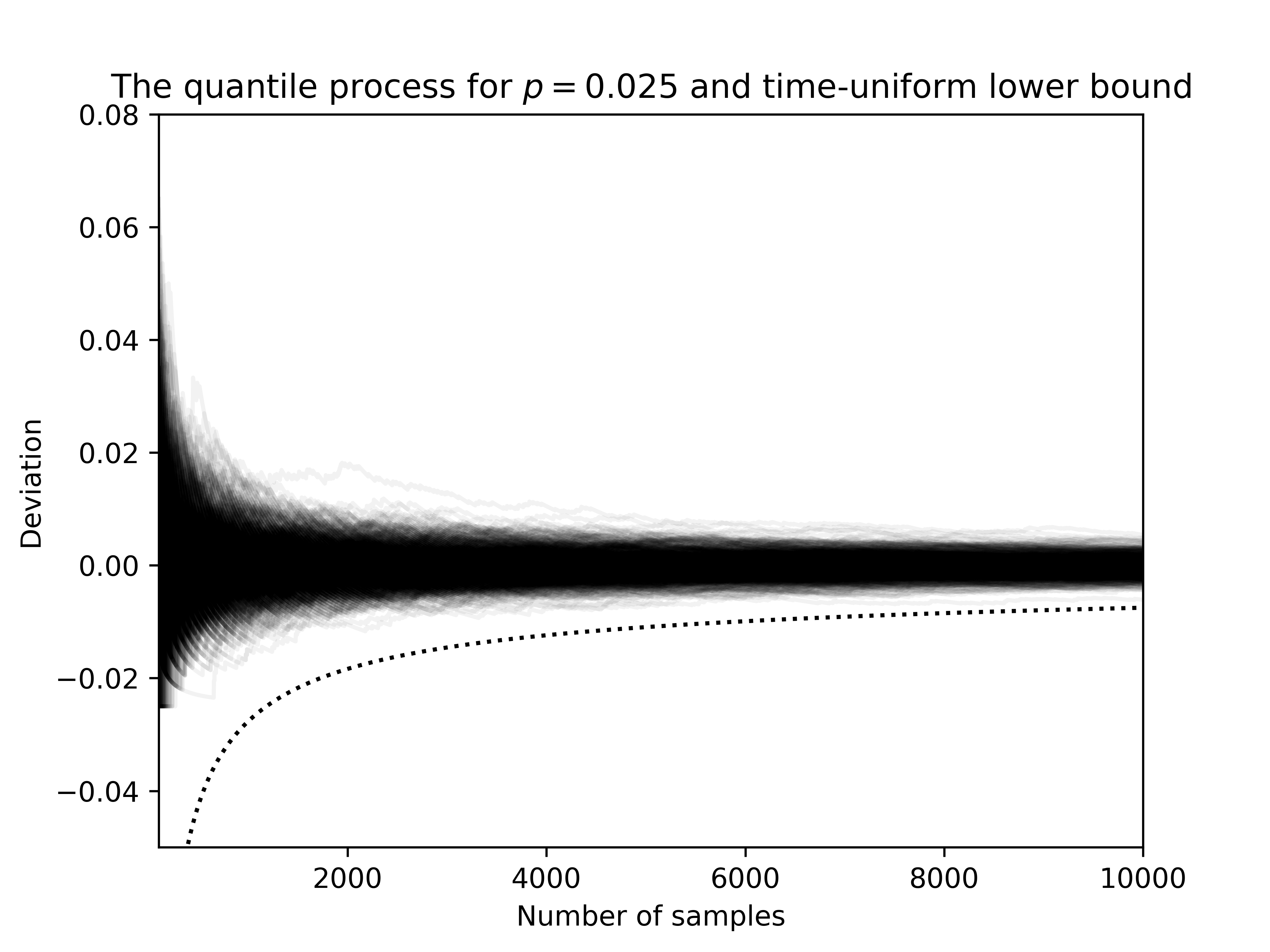
Figure 1. Some trajectories of the quantile process and the time-uniform bound provided in [2].

To begin, we recall the notation of [2] and define

$$S_{t}=\sum_{i=1}^{t}(\mathbb{I}_{X_{i}\leq Q(p)}-p)$$ (2.1)

where $X_{i}\sim F$ is an i.i.d. sequence and $Q(p)$ is the $p$ quantile w.r.t. $F$. We note that by definition $\widehat{F}_{t}(Q(p))=S_{t}/t$, as such, if we can find a function $-p<f(t,p,\delta)<0$ such that

$$\mathbb{P}(\exists t:\,S_{t}/t<f(t,p,\delta))\leq\delta$$ (2.2)

it would imply by the definition of the quantile function, that

$$\mathbb{P}(\exists t:\,Q(p)<\widehat{Q}_{t}(p+f(t,p,\delta)))\leq\delta.$$ (2.3)

Thus, if we wish to have a lower bound on a quantile (think small quantile), we can study the Bernoulli process $S_{t}$. In order to explain the simulation setup we begin by requiring that we have an initial waiting time $m$ and a cutoff-time $M$ (for the simulation), and consider

$$\mathbb{P}(\exists t:\,S_{t}/t<f(t,p,\delta))\leq\mathbb{P}(\exists t\in[m,M]:\,S_{t}/t<f(t,p,\delta))\\ +\mathbb{P}(\exists t>M:\,S_{t}/t<f(t,p,\delta))$$

The first term we will handle via simulation and the second term will be analytically bounded using the following quantile specific version of Theorem 1, which can be found in [2]:

Theorem 4.

For any $p,\delta\in(0,1)$, $s,\eta>1$, and $M\geq 1$, we have

$$\mathbb{P}(\exists t\geq M:Q(p)<\widehat{Q}_{t}(p-g(t,M,p,\delta)))\leq\delta$$

with

$$g(t,M,p,\delta)=\sqrt{k_{1}^{2}p(1-p)tl(t)+k_{2}^{2}c_{p}^{2}l^{2}(t)}+c_{p}k_{2}l(t)$$

where

$$\begin{cases}l(t)=s\log(\log(\eta t/M))+\log(2\zeta(s)/(\delta\log^{s}\eta))\\ k_{1}=(\eta^{1/4}+\eta^{-1/4})/\sqrt{2}\\ k_{2}=(\sqrt{\eta}+1)/2\\ c_{p}=(1-2p)/3,\end{cases}$$

where $\zeta$ is the Riemann zeta function.

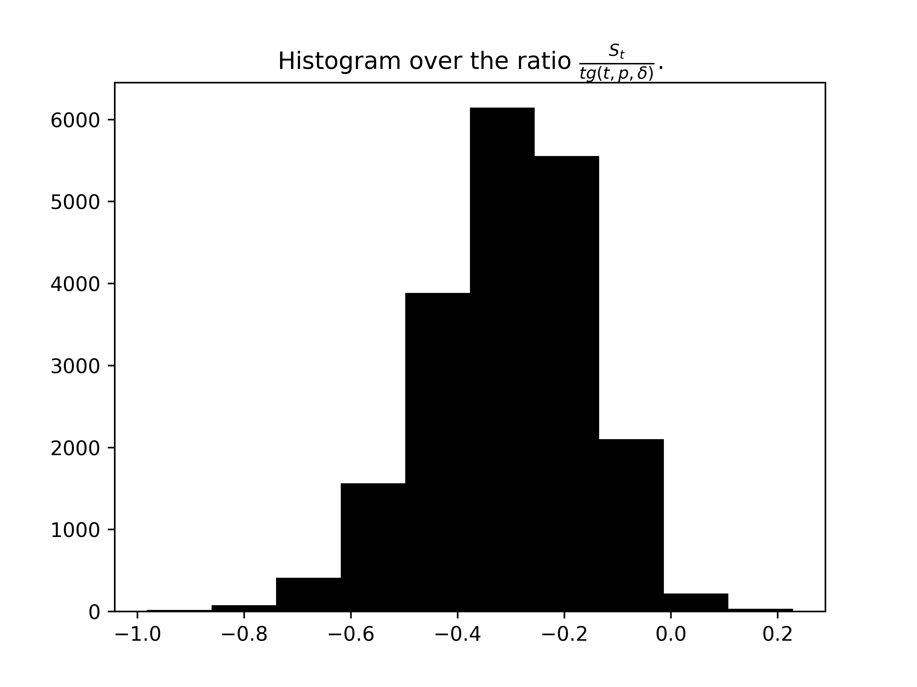
Figure 2. Histogram over $c_{Z}$.

We now start by defining the random variable

$$Z=\min_{t\in[m,M]}\frac{S_{t}}{tg(t,p,\delta/2)}$$

where the function $g$ is given in Theorem 4 with some fixed parameters, we have chosen the same as in [2], namely $\eta=2.04$ and $s=1.4$. The goal of the simulation is to estimate the $\delta/2$ quantile of $Z$ (see Fig. 2). If we consider an empirical quantile $\widehat{Q}_{t,Z}(\delta/2)$, formed using $t$ i.i.d. copies of $Z$ which we denote $\mathbf{Z}_{t}$, then using Lemma A.1 we get that for any $\widetilde{\delta}\in(0,1)$,

$$\mathbb{P}(\mathbb{P}(\widetilde{Z}\leq\widehat{Q}_{t,\mathbf{Z}_{t}}(\delta/2-\epsilon(t,\delta/2,\widetilde{\delta}))\mid\mathbf{Z}_{t})\leq\delta/2)\geq 1-\widetilde{\delta}$$

where $\widetilde{Z}$ is an independent copy of $Z$. Translating this back to the quantile process we obtain

$$\mathbb{P}\bigg{[}\mathbb{P}\big{(}\exists t\in[m,M]:\,\widehat{F}_{t}(Q(p))<\widehat{Q}_{t,\mathbf{Z}_{t}}\bigg{(}\frac{\delta}{2}-\epsilon\big{(}t,\frac{\delta}{2},\widetilde{\delta}\big{)}\bigg{)}g\big{(}t,p,\frac{\delta}{2}\big{)}\mid\mathbf{Z}_{t}\big{)}\leq\frac{\delta}{2}\bigg{]}\geq 1-\widetilde{\delta}.$$

Thus, the introduction of the simulation step makes the quantile confidence statement of a $2$-parameter PAC type, as described for the prediction interval. If we later employ this in the same way as we did before but for the prediction interval we will have a $3$-parameter PAC statement. We can see how this sharpens the bounds in Fig. 3.

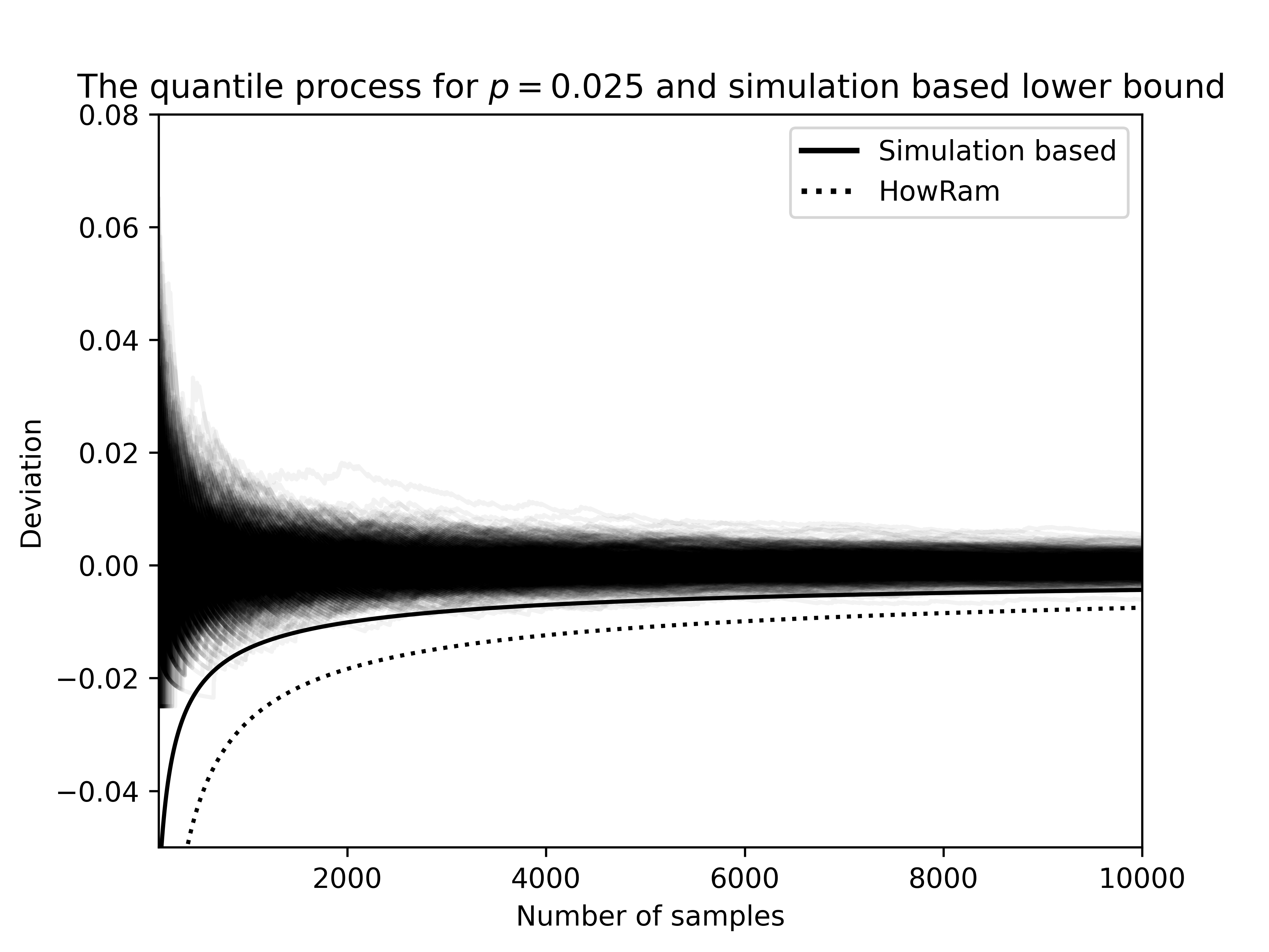
Figure 3. Quantile process with a simulated quantile compared to the bound obtained by Theorem 4.

If we denote $c_{Z}=-\widehat{Q}_{t,\mathbf{Z}_{t}}(\delta/2-\epsilon(t,\delta/2,\widetilde{\delta}))$ (think of $c_{Z}>0$) and $g_{t}=g(t,p,\delta/2)$, then the above can be written more compactly as

$$\mathbb{P}(\mathbb{P}(\exists t\in[m,M]:\,S_{t}/t<-c_{Z}g_{t}\mid\mathbf{Z}_{t})\leq\delta/2)\geq 1-\widetilde{\delta}.$$

Define now the $\mathbf{Z}_{t}$ dependent event

$$A=\{Q_{Z}(\delta/2)\geq\widehat{Q}_{t,\mathbf{Z}_{t}}(\delta/2-\epsilon(t,\delta/2,\widetilde{\delta}))\},$$

then, on $A$ we have

$$\mathbb{P}(\exists t\in[m,M]:\,S_{t}/t<-c_{Z}g_{t})\leq\delta/2.$$

Using the union bound we can estimate on the event $A$

$$\mathbb{P}(\exists t\geq m:S_{t}/t<-\mathbb{I}_{t\leq M}c_{Z}g_{t}-\mathbb{I}_{t>M}g(t,M,p,\delta/2))\\ \leq\mathbb{P}(\exists t\in[m,M]:S_{t}/t<-c_{Z}g_{t})+\mathbb{P}(\exists t>M:S_{t}/t<-g(t,M,p,\delta/2))\leq\delta$$

Example 2.1.

For $p=0.05,\delta=0.05,m=10,\widetilde{\delta}=0.0000001$, and $M=10000$ we obtain that $c_{Z}$ is roughly $0.6$ and that parameters $\eta,s$ can be chosen such that $g(M,M,p,\delta/2)$ is essentially the same size as $c_{Z}g_{M}$.

Assembling everything we finally get,

$$\mathbb{P}(\mathbb{P}(\exists t\geq m:\widehat{F}_{t}(Q(p))<p-\mathbb{I}_{t\leq M}c_{Z}g_{t}-\mathbb{I}_{t>M}g(t,M,p,\delta/2)\mid\mathbf{Z}_{t})\leq\delta)\geq 1-\widetilde{\delta}$$ (2.4)

We can compare the bounds obtained in Fig. 4 for our particular choices.

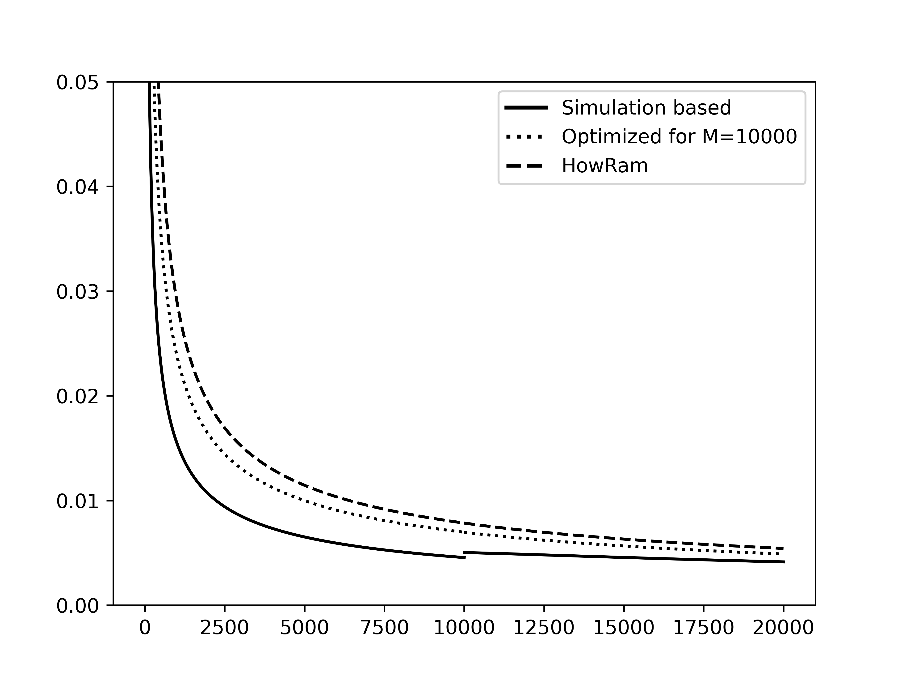
Figure 4. Comparison of the different bounds.

2.1. $3$-parameter PAC for prediction intervals

Combining the arguments leading to 2.4 and 1.4 we can redefine the event $A$ to be (where we have defined $Z$ w.r.t. $p=\alpha/2$)

$$A=\{Q_{Z}(\delta/4)\geq\widehat{Q}_{t,\mathbf{Z}_{t}}(\delta/4-g(t,\delta/4,\widetilde{\delta}))\},$$

then the event $A$ happens with probability $1-\widetilde{\delta}$. On the event $A$ we then obtain that our prediction interval can be taken to be

$$C^{l,\alpha}_{i} =[\widehat{Q}_{i}(\alpha/2-|c_{Z}|g_{i}),\widehat{Q}_{i}^{-}(1-\alpha/2+|c_{Z}|g_{i})]$$ (2.5)

and on the event $A$ we have the following version of 1.4

$$\mathbb{P}(\forall i:\mathbb{P}(X\in C^{l,\alpha}_{i})\geq 1-\alpha)\geq 1-\delta.$$ (2.6)

This constitutes a $3$-parameter PAC definition with parameters $(\widetilde{\delta},\delta,\alpha)$, where the first can be taken as small as we wish at the cost of our simulation.

3. Application examples

In this section we will apply our $3$-parameter PAC formulation for prediction intervals in conjunction with what is developed in Section 1.2. The first example is the following regression problem

$$r(x):=\mathbb{E}[Y\mid X=x]=\sin(3x)$$

$$\sigma(x):=\sqrt{\mathbb{V}[Y\mid X=x]}=|\sin(10x)|.$$

We assume that

$$Y=r(X)+\sigma(X)\epsilon,\quad\epsilon\sim N(0,1),$$

and that $X\sim\text{unif}([0,1])$. We estimate $r$ using the Nadaraya-Watson estimator with Gaussian kernel of bandwidth $1/500$ and estimate $\sigma(x)$ using again a Nadaraya-Watson estimator as in Appendix B. We then construct the score function

$$S=\frac{Y-r(X)}{\sigma(X)}$$

and construct a prediction interval for $S$, then this is used to construct a prediction interval for $Y$. We can see the result in Fig. 5.

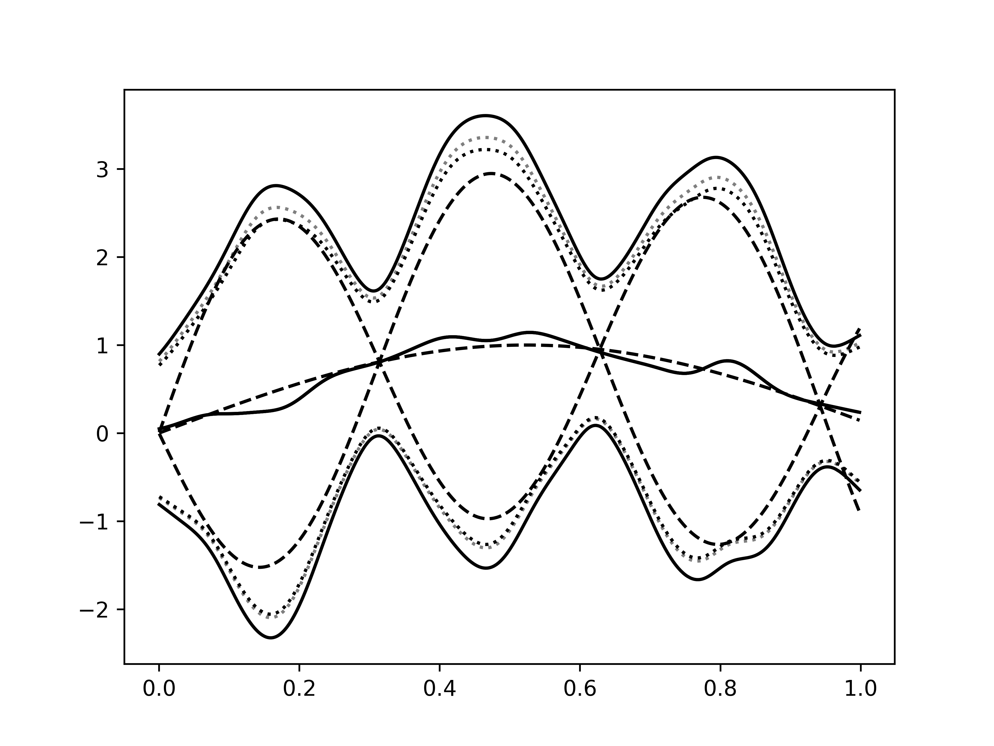
Figure 5. Simulation of the regression problem. The solid lines are the upper and lower limit of the prediction interval using the $2$-PAC definition and the dotted lines represent the intervals with the $3$-PAC definition for increasing number of samples. The dashed lines represent the true regression function as well as the true conditional quantiles.

Since our method of constructing prediction intervals is asymmetric we can have a skew distribution for $\epsilon$, in Fig. 6 we see the corresponding result when $\epsilon$ is assumed to be a standardized log-Normal.

We can see an example of the estimated coverage as we keep adding data in Fig. 7

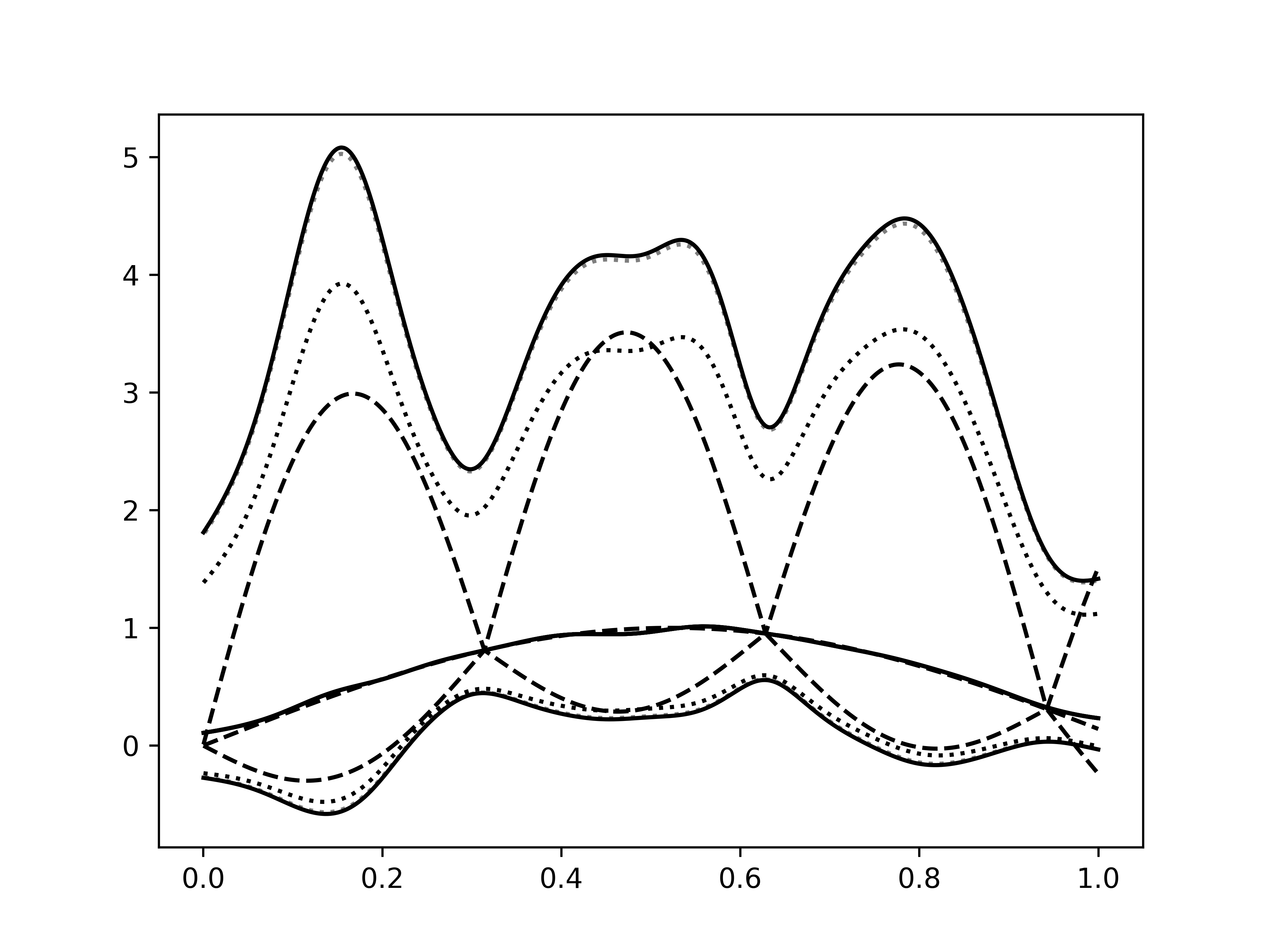
Figure 6. Simulation of the skew regression problem. The solid lines are the upper and lower limit of the prediction interval using the $2$-PAC definition and the dotted lines represent the intervals with the $3$-PAC definition for increasing number of samples. The dashed lines represent the true regression function as well as the true conditional quantiles.

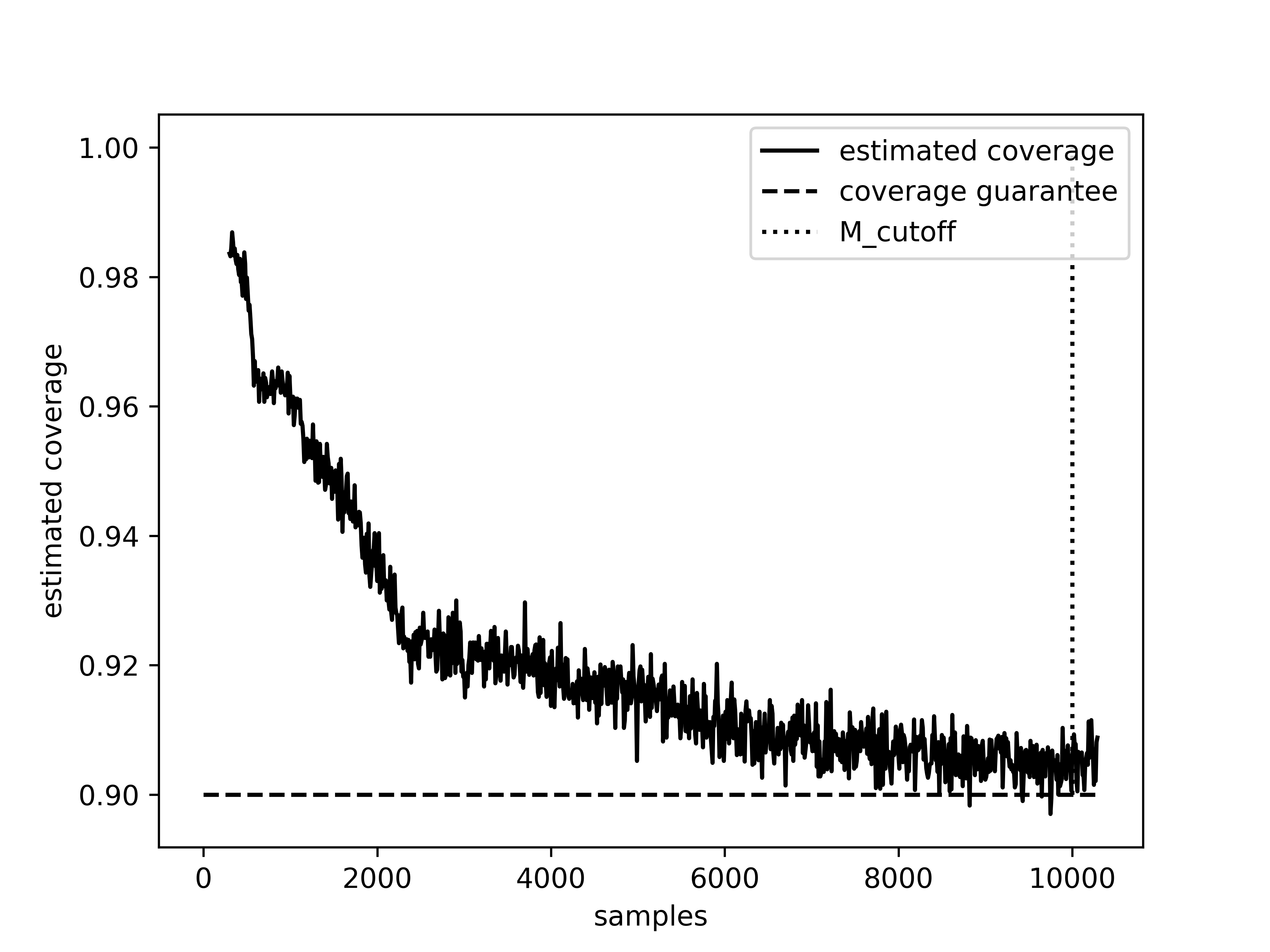
Figure 7. Estimated coverage of the log-Normal noise using the 3-parameter PAC in Section 2.1.

If we instead of relying on the 3-parameter PAC we use Theorem 2, we get also the data-dependent upper bound on the true coverage. A resulting simulation can be found in Fig. 8.

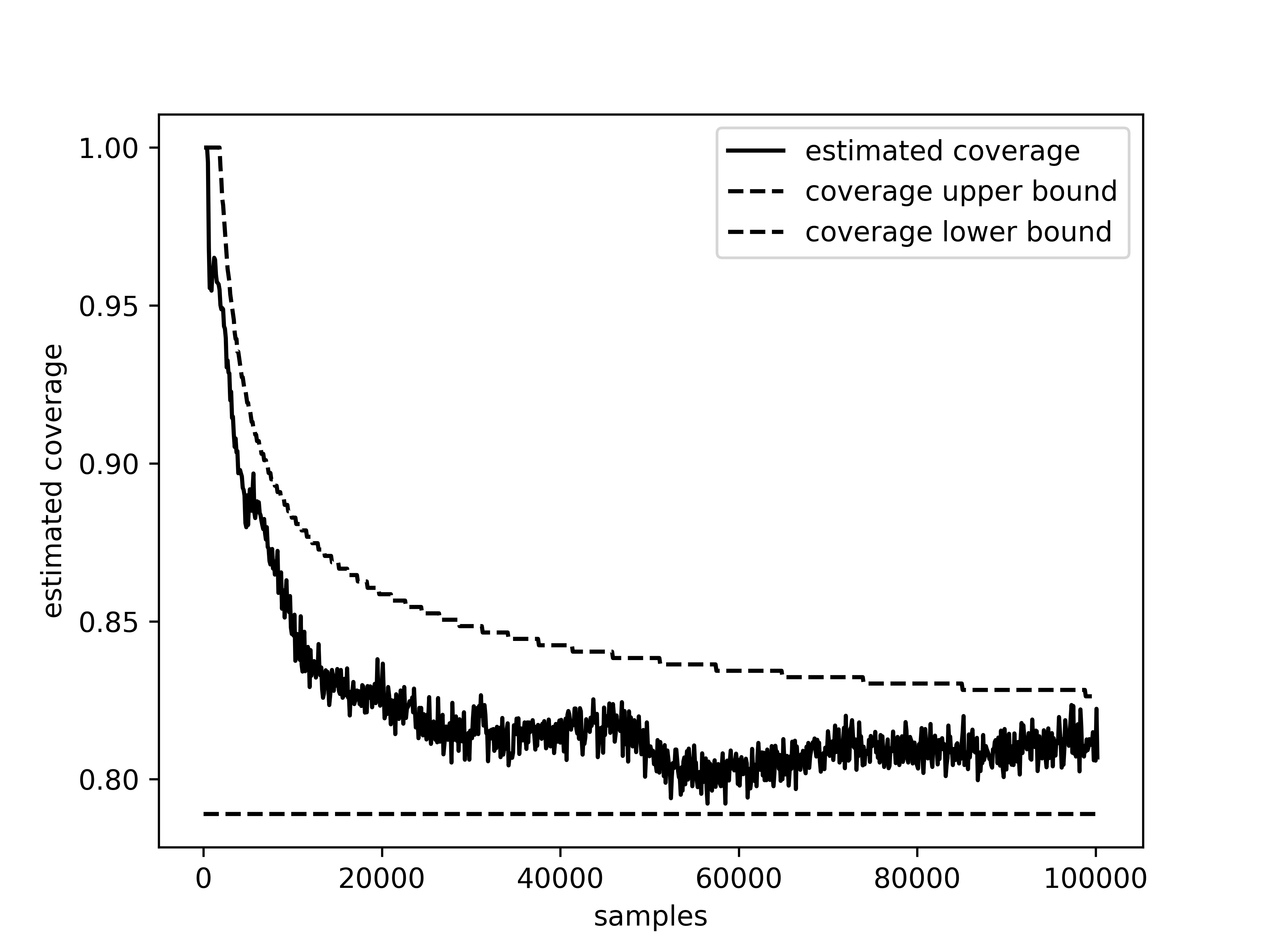
Figure 8. Estimated coverage using Theorem 2.

Appendix A Helper lemmas

Theorem 5 (Bennett’s inequality).

Let $X_{1},\ldots,X_{n}$ be i.i.d. random variables with finite variance such that $\mathbb{P}(X_{i}\leq b)=1$ with mean zero. Let and $\sigma^{2}=\mathbb{V}[X_{i}]$. Then for any $\epsilon>0$,

$$\mathbb{P}(\overline{X}_{n}\geq\epsilon)\leq\exp\left(-\frac{n\sigma^{2}}{b^{2}}h\left(\frac{b\epsilon}{\sigma^{2}}\right)\right)$$

where $h(u)=(1+u)\log(1+u)-u$ for $u>0$.

Lemma A.1.

Let $Z_{1},\ldots$ be an i.i.d. sequence of random variables, let $Q$ and $F$ be the quantile function and distribution function respectively, then

$$\mathbb{P}(Q(p)\leq\widehat{Q}_{t}(p-\epsilon))\leq\exp\left(-tp(1-p)h\left(\frac{\epsilon}{p(1-p)}\right)\right)$$

where $h(u)=(1+u)\log(1+u)-u$ for $u>0$. Thus for a given $\delta>0$ we can find $\epsilon(t,p,\delta)$ such that

$$\mathbb{P}(Q(p)\leq\widehat{Q}_{t}(p-\epsilon(t,p,\delta)))\leq\delta$$

Proof.

First note that by the definition of the quantile function, we have

$$\mathbb{P}(Q(p)\leq Q_{t}(p-\epsilon))= \mathbb{P}(\widehat{F}_{t}(Q(p))\leq\widehat{F}_{t}(Q_{t}(p-\epsilon)))$$

$$\leq \mathbb{P}\left(\frac{1}{t}\sum_{i=1}^{t}\mathbb{I}_{\{Z_{i}\leq Q(p)\}}\leq p-\epsilon\right)$$

Now $X_{i}=\mathbb{I}_{\{Z_{i}\leq Q(p)\}}$ is an i.i.d. sequence of Bernoulli random variables with probability $p$, thus an application of Theorem 5 gives the result. ∎

Appendix B Nadaraya-Watson for variance

The basis for the classical Nadaraya-Watson estimator is to first estimate the joint density of the pair $(X,Y)\sim F_{XY}$, where $X,Y\in\mathbb{R}$, using a Kernel density estimator. The Nadaraya-Watson estimator is then nothing but the regression function $\mathbb{E}[Y\mid X]$, where the expectation is taken with respect to the estimated density. Similarly we can estimate the conditional variance, namely we can estimate $\mathbb{V}[Y\mid X]$ by computing it using the estimated density. Here we provide the calculation for reference:

We begin by selecting a kernel $K_{h}:\mathbb{R}\to\mathbb{R}_{+}$ such that $\int K_{h}(x)dx=1$, $\int xK_{h}(x)dx=0$ and $\int x^{2}K_{h}(x)dx=h^{2}$, i.e. a non-negative function, a classical choice is the Gaussian. Having now an i.i.d. sequence of observations $Z_{i}=(X_{i},Y_{i})$, for $i=1,\ldots,n$ we construct the kernel density estimator as

$$\widehat{\rho}_{n}(z)=\frac{1}{n}\sum_{i=1}^{n}K_{h}(x-X_{i})K_{h}(y-Y_{i}).$$

From this definition we compute

$$\mathbb{V}_{\widehat{\rho}_{n}}[Y\mid X]=\int y^{2}\frac{\widehat{\rho}_{n}(z)}{\int\widehat{\rho}(x,y)dy}dy-\mathbb{E}_{\widehat{\rho}_{n}}[Y|X]^{2}.$$

From which we see that we first need to compute

$$\int\widehat{\rho}(x,y)dy =\int\frac{1}{n}\sum_{i=1}^{n}K_{h}(x-X_{i})K_{h}(y-Y_{i})dy$$

$$=\frac{1}{n}\sum_{i=1}^{n}K_{h}(x-X_{i})$$

Furthermore,

$$\int y^{2}\frac{\widehat{\rho}_{n}(z)}{\int\widehat{\rho}(x,y)dy}dy =\frac{1}{n}\sum_{i=1}^{n}\int y^{2}\frac{K_{h}(x-X_{i})K_{h}(y-Y_{i})}{\frac{1}{n}\sum_{j=1}^{n}K_{h}(x-X_{j})}dy$$

$$=\frac{1}{n}\sum_{i=1}^{n}\frac{K_{h}(x-X_{i})}{\frac{1}{n}\sum_{j=1}^{n}K_{h}(x-X_{j})}\int y^{2}K_{h}(y-Y_{i})dy$$

$$=\frac{\sum_{i=1}^{n}K_{h}(x-X_{i})(h^{2}+Y_{i}^{2})}{\sum_{j=1}^{n}K_{h}(x-X_{j})}$$

thus we conclude that the Nadaraya-Watson kernel estimator of variance is

$$\mathbb{V}_{\widehat{\rho}_{n}}[Y\mid X]=\frac{\sum_{i=1}^{n}K_{h}(x-X_{i})(h^{2}+Y_{i}^{2})}{\sum_{j=1}^{n}K_{h}(x-X_{j})}-\left(\frac{\sum_{i=1}^{n}K_{h}(x-X_{i})Y_{i}}{\sum_{j=1}^{n}K_{h}(x-X_{j})}\right)^{2}.$$

References

[1]A. Gammerman, V. Vovk and V. Vapnik
“Learning by Transduction”
In Proceedings of the Fourteenth Conference on Uncertainty in Artificial Intelligence, UAI’98
Madison, Wisconsin: Morgan Kaufmann Publishers Inc., 1998, pp. 148–155
[2]Steven R Howard and Aaditya Ramdas
“Sequential estimation of quantiles with applications to A/B testing and best-arm identification”
In Bernoulli28.3Bernoulli Society for Mathematical StatisticsProbability, 2022, pp. 1704–1728
[3]Jing Lei and Larry Wasserman
“Distribution-free prediction bands for non-parametric regression”
In Journal of the Royal Statistical Society Series B: Statistical Methodology76.1Oxford University Press, 2014, pp. 71–96
[4]Harris Papadopoulos, Kostas Proedrou, Volodya Vovk and Alex Gammerman
“Inductive confidence machines for regression”
In Machine Learning: ECML 2002: 13th European Conference on Machine Learning Helsinki, Finland, August 19–23, 2002 Proceedings 13, 2002, pp. 345–356
Springer
[5]Leslie G Valiant
“A theory of the learnable”
In Communications of the ACM27.11ACM New York, NY, USA, 1984, pp. 1134–1142
[6]Vladimir Vovk
“Conditional validity of inductive conformal predictors”
In Asian conference on machine learning, 2012, pp. 475–490
PMLR
[7]Vladimir Vovk, Alexander Gammerman and Glenn Shafer
“Algorithmic learning in a random world”
Springer, 2005