Steering is a type of nonseparable quantum correlation, where its inherent asymmetric feature makes it distinct from Bell-nonlocality and entanglement. In this paper, we investigate quantum steering in a two-mode Gaussian state $\hat{\varrho}_{c_{1}c_{2}}$ coupled to a two-mode vacuum reservoir. The mode $c_{1}$($c_{2}$) is emitted during the first(second) transition of a nondegenerate three-level cascade laser. By means of the master equation of the state $\hat{\varrho}_{c_{1}c_{2}}$, we derive analytical expression of the steady-state covariance matrix of the modes $c_{1}$ and $c_{2}$. Using realistic experimental parameters, we show that the state $\hat{\varrho}_{c_{1}c_{2}}$ can exhibit asymmetric steering. Furthermore, by an appropriate choice of the physical parameters of the state $\hat{\varrho}_{c_{1}c_{2}}$, we show that one-way steering can be achieved. Essentially, we demonstrate that one-way steering can, in general, occur only from $c_{1}\rightarrow c_{2}$. Besides, we perform a comparative study between the steering of the two laser modes and their Gaussian Rényi-2 entanglement. As results, we found that the entanglement and steering behave similarly in the same circumstances, i.e., both of them decay under dissipation effect, moreover, they can be well enhanced by inducing more and more quantum coherence in the state $\hat{\varrho}_{c_{1}c_{2}}$. In particular, we found that the steering remains always less than the Gaussian Rényi-2 entanglement.

1 Introduction

The aspect of quantum steering was first introduced by E. Schrödinger [1, 2] in order to capture the essence of the Einstein-Podolsky-Rosen paradox [3]. According to E. Schrödinger, steering is a quantum phenomenon that allows one observer (say Alice) to remotely affect the state of another observer (say Bob) via local operations [4].

In the hierarchy of nonseparable quantum correlations [4], steering stands between entanglement [5] and Bell nonlocality [6]. From an operational point of view, in a bipartite quantum state $\hat{\varrho}_{XY}$, violation of the Bell inequality implies that the state is steerable in both directions $X\rightleftarrows Y$, while, demonstrating steering at least in one direction ($X\rightarrow Y$) or ($Y\rightarrow X$) makes sure that the state is entangled.

In quantum information precessing [7], quantum steering corresponds to the task of verifiable entanglement distribution by an untrusted observer [4]. In other words, if two observers Alice and Bob share a bipartite state which is steerable (saying) from Alice$\rightarrow$Bob, therefore, Alice can convince Bob that their shared bipartite state is entangled by implementing local measurements and classical communications [4]. Unlike entanglement, quantum steering is an asymmetric form of quantum correlations, i.e., a bipartite state $\hat{\varrho}_{XY}$ may be steerable solely in one direction, which is referred to as one-way quantum steering [8].

To probe quantum steering in bipartite quantum states, various criteria have been proposed. We cite for instance, the Reid criterion [9], the Cavalcanti criterion [10], the Costa criterion [11], and the Wolmann criterion [12]. In particular, within the Gaussian framework [13], Kogias and the co-authors [8] have proposed a computable measure to quantify the amount by which a bipartite state is steerable in a given direction under Gaussian measurements. Also, they showed that in an arbitrary two-mode Gaussian state, the proposed measure cannot exceed entanglement when the later is defined via the Gaussian Rényi-2 entropy [14, 15].

Nowadays, it is believed that the key ingredient of asymmetric quantum information tasks—where some of the parties are untrusted—is quantum steering [16]. For example, quantum steering has been recognized as the essential resource for one-sided device-independent (1SDI) quantum key distribution [17], quantum secret sharing [18], quantum teleportation [19], one-way quantum computing [20], and sub-channel discrimination [21].

Gaussian quantum steering has been studied in various systems [22, 23, 24, 25, 26, 27, 28, 29, 30, 31, 32, 33]. To the best of our knowledge, no previous work considering a nondegenerate three-level laser coupled to two-mode vacuum reservoir has analyzed asymmetric Gaussian steering.

Motivated by the considerable attention that has recently been paid to quantum steering as the key ingredient in the implementation of asymmetric quantum information tasks, we investigate, under realistic experimental conditions, Gaussian quantum steering of two optical modes (labelled as $c_{1}$ and $c_{2}$) generated by a nondegenerate three-level cascade laser. For this, we use the measure proposed by Kogias et al. [8] to quantify the amount by which the two-mode Gaussian state $\hat{\varrho}_{c_{1}c_{2}}$ is steerable in a given direction. Furthermore, we compare, under the same circumstances, the steering of the two considered modes with their corresponding entanglement quantified by means of the Gaussian Rényi-2 entanglement. We emphasize that our interest in Gaussian states is motivated on the one hand by the fact that such states admit a simple mathematical description, and on the other hand by the fact that they can be reliably generated and manipulated in a variety of experimental platforms [13]. Importantly, Gaussian measurements can be effectively implemented by means of homodyne detections [34].

Extensive researches have been carried out on the quantum analysis of the light generated by a nondegenerate three-level laser [35]. These researches reveal that the two laser modes, emitted during a cascade transition, exhibit strong non-classical correlations between them [36], which is exploited to study, e.g., entanglement, quantum bistability [37], squeezing [38] and the statistical properties of the light [39].

A nondegenerate three-level cascade laser can be defined as a quantum system constituted by a set of nondegenerate three-level atoms, which are initially prepared in a quantum coherent superposition of the top and bottom levels inside a cavity [40].

In such system, the fundamental role is played by the quantum coherence, that can be achieved either by an initial preparation of the atoms in a coherent quantum superposition of the top and bottom levels [41], or by coupling these two levels by means of strong laser field [42]. When a single atom passes from the top to bottom level through the intermediate level, two photons are created. If the two emitted photons are identical (i.e., have the same frequency), the laser is referred to as a degenerate three-level laser, and a nondegenerate three-level laser otherwise.

The remainder of this paper is organized as follows. In Sec. 2, we introduce the studied system, and by applying the master equation of the two-mode Gaussian state $\hat{\varrho}_{c_{1}c_{2}}$, we calculate the dynamics of the first and second moments of the two laser modes variables. Also, we analytically evaluate the steady-state covariance matrix fully describing the two-mode Gaussian state $\hat{\varrho}_{c_{1}c_{2}}$. In Sec. 3, using realistic experimental parameters, we study Gaussian quantum steering of the two laser modes $c_{1}$ and $c_{2}.$ Furthermore, we compare the steering of the modes $c_{1}$ and $c_{2}$ with their corresponding entanglement quantified by means of the Gaussian Rényi-2 entanglement. Finally, in Sec. 4, we draw our conclusions.

2 Model and master equation

Inside a doubly resonant cavity, we consider a set of nondegenerate three-level atoms in interaction with two optical modes of the quantized cavity field [35]. The first(second) optical mode is specified by its annihilation operator ($\hat{c}_{1}$)$\hat{c}_{2}$, frequency ($\omega_{c_{1}}$)$\omega_{c_{2}}$ and dissipation rate ($\kappa_{1}$)$\kappa_{2}$. We assume that the atoms are injected into the cavity with a constant rate $\rho$ and removed during a time $\tau$ [39]. As illustrated in Fig. 1, the upper, intermediate and lower energy levels of a single nondegenerate three-level atom are denoted, respectively, by $|u\rangle,$ $|i\rangle$ and $|l\rangle$.

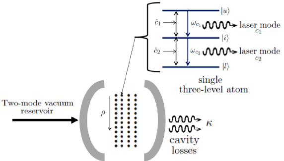
Figure 1: Schematic representation of a nondegenerate three-level laser coupled to a two-mode vacuum reservoir [45]. $|u\rangle$, $|i\rangle$, and $|l\rangle$ denote, respectively, the upper, intermediate, and lower energy levels for a single three-level atom. The transition from $|u\rangle\rightarrow|i\rangle$($|i\rangle\rightarrow|l\rangle$), at frequency $\omega_{c_{1}}$($\omega_{c_{2}}$) and spontaneous emission decay rate $\gamma_{ul}$($\gamma_{li}$), is considered to be in resonance with the quantized cavity modes $c_{1}$($c_{2}$). Whereas, the transition from $|u\rangle\rightarrow|i\rangle$ is dipole forbidden [36]. The gain medium of the laser is an ensemble of three-level atoms in a cascade configuration. The atoms are assumed to be initially prepared in a coherent superposition of the upper and lower levels, and injected into the cavity with a constant rate $\rho$.

Under the rotating wave approximation, the two optical modes $c_{1}$ and $c_{2}$ and a single three-level atom can be described by the following Hamiltonian [35]

$$\mathcal{\hat{H}}_{\mathrm{int}}=\mathrm{i}\hbar\left(\epsilon_{ui}\hat{c}_{1}|u\rangle\langle i|+\epsilon_{il}\hat{c}_{2}|i\rangle\langle l|-\epsilon_{ui}|i\rangle\langle u|\hat{c}_{1}^{{\dagger}}-\epsilon_{il}|l\rangle\langle i|\hat{c}_{2}^{{\dagger}}\right),$$ (1)

where int stands for interaction picture. $\epsilon_{ui}$ and $\epsilon_{il}$ being the coupling constants corresponding to the transitions $|u\rangle\rightarrow|i\rangle$ and $|i\rangle\rightarrow|l\rangle$, respectively [39]. The atoms are also assumed to be initially prepared in an arbitrary quantum coherent superposition of the upper $|u\rangle$ and lower $|l\rangle$ energy levels [43]. With this assumption, the initial state of a single atom as well as its associated density operator, respectively, read

$$|\Psi_{\mathrm{sa}}(0)\rangle = P_{u}|u\rangle+P_{l}|l\rangle$$ (2)

$$\hat{\varrho}_{\mathrm{sa}}(0) = \varrho_{uu}^{(0)}|u\rangle\langle u|+\varrho_{ul}^{(0)}|u\rangle\langle l|+\varrho_{lu}^{(0)}|l\rangle\langle u|+\varrho_{ll}^{(0)}|l\rangle\langle l|,$$ (3)

where sa stands for single atom. In the last equation, $\varrho_{uu}^{(0)}=|P_{u}|^{2}$ and $\varrho_{ll}^{(0)}=|P_{l}|^{2}$ represent the probabilities for a single three-level atom to be initially in the upper and lower levels, respectively, while $\varrho_{ul}^{(0)}=\varrho_{lu}^{(0)\ast}=P_{u}P_{l}^{\ast}$ is the initial quantum coherence of a single three-level atom [44]. From now on, without affecting the generality of our study, we take identical spontaneous decay rates for both transitions $|u\rangle\rightarrow|i\rangle$ and $|i\rangle\rightarrow|l\rangle$, i.e., $\gamma_{ui}=\gamma_{il}=\gamma$, identical coupling transitions, i.e., $\epsilon_{ui}=\epsilon_{il}=\epsilon$, and identical cavity decay rates $\kappa_{1}=\kappa_{2}=\kappa.$

The master equation for the reduced density operator $\hat{\varrho}_{c_{1}c_{2}}\equiv\hat{\varrho}$ of the two laser modes $c_{1}$ and $c_{2}$, reads [46, 47]

$$\partial_{t}\hat{\varrho}=\frac{-\mathrm{i}}{\hbar}\mathrm{Tr}_{\mathrm{sa}}\left[\mathcal{\hat{H}}_{\mathrm{int}},\hat{\varrho}_{\{\mathrm{sa+field}\}}\right]+\sum\limits_{j=1,2}\frac{\kappa_{j}}{2}\mathcal{L}\left[\hat{c}_{j}\right]\hat{\varrho},$$ (4)

where $\hat{\varrho}_{\{\mathrm{sa+field}\}}$ is the density matrix that describes a single atom plus the two-mode cavity field, and the Lindblad operator $\mathcal{L}\left[\hat{c}_{j}\right]\hat{\varrho}=2\hat{c}_{j}\hat{\varrho}\hat{c}_{j}^{{\dagger}}-\left[\hat{c}_{j}^{{\dagger}}\hat{c}_{j},\hat{\varrho}\right]_{+}$ is added to describe the damping of the $j$-th laser mode in the vacuum reservoir.

In the good cavity limit $\gamma\gg\kappa$, and the linear-adiabatic approximation [48], one can show—after some tedious but straightforward algebra—that Eq. (4) would be [49, 50]

$$\partial_{t}\hat{\varrho} = \frac{A\varrho_{uu}^{(0)}}{2}[2\hat{c}_{1}^{{\dagger}}\hat{\varrho}\hat{c}_{1}-\hat{c}_{1}\hat{c}_{1}^{{\dagger}}\hat{\varrho}-\hat{\varrho}\hat{c}_{1}\hat{c}_{1}^{{\dagger}}]+\frac{A\varrho_{ll}^{(0)}}{2}[2\hat{c}_{2}\hat{\varrho}\hat{c}_{2}^{{\dagger}}-\hat{c}_{2}^{{\dagger}}\hat{c}_{2}\hat{\varrho}-\hat{\varrho}\hat{c}_{2}^{{\dagger}}\hat{c}_{2}]+$$ (5)

$$\frac{A\varrho_{ul}^{(0)}}{2}[\hat{\varrho}\hat{c}_{1}^{{\dagger}}\hat{c}_{2}^{{\dagger}}+\hat{c}_{1}^{{\dagger}}\hat{c}_{2}^{{\dagger}}\hat{\varrho}+\hat{c}_{1}\hat{c}_{2}\hat{\varrho}+\hat{\varrho}\hat{c}_{1}\hat{c}_{2}-2\hat{c}_{1}^{{\dagger}}\hat{\varrho}\hat{c}_{2}^{{\dagger}}-2\hat{c}_{2}\hat{\varrho}\hat{c}_{1}]+\sum\limits_{j=1,2}\frac{\kappa}{2}\mathcal{L}\left[\hat{c}_{j}\right]\hat{\varrho},$$

where we choice $\varrho_{ul}^{(0)}$ to be real for simplicity. The linear gain coefficient $A=2\rho\epsilon^{2}/\gamma^{2}$ describes the rate at which the three-level atoms are injected into the cavity [51]. In the above equation, the term proportional to $\varrho_{uu}^{(0)}$($\varrho_{ll}^{(0)}$) represents the gain(loss) of the laser mode $c_{1}$($c_{2}$), whereas the term proportional to $\varrho_{ul}^{(0)}$ represents the coupling between these two laser modes due to the quantum coherence [35]. Now, using Eq. (5) and the formula $\partial_{t}\langle\mathcal{\hat{O}}(t)\rangle=\mathrm{Tr}(\partial_{t}\hat{\varrho}\mathcal{\hat{O}}(t))$, we obtain the dynamics of the first and second moments of the laser modes variables,

$$\partial_{t}\langle\hat{c}_{j}(t)\rangle = \frac{-\Gamma_{j}}{2}\langle\hat{c}_{j}(t)\rangle+\frac{\left(-1\right)^{j}A\varrho_{ul}^{(0)}}{2}\langle\hat{c}_{3-j}^{{\dagger}}(t)\rangle,\text{ for }j=1,2\text{,}$$ (6)

$$\partial_{t}\langle\hat{c}_{j}^{2}(t)\rangle = -\Gamma_{j}\langle\hat{c}_{j}^{2}(t)\rangle+\left(-1\right)^{j}A\varrho_{ul}^{(0)}\langle\hat{c}_{1}(t)\hat{c}_{2}^{{\dagger}}(t)\rangle,$$ (7)

$$\partial_{t}\langle\hat{c}_{j}^{{\dagger}}(t)\hat{c}_{j}(t)\rangle = -\Gamma_{j}\langle\hat{c}_{j}^{{\dagger}}(t)\hat{c}_{j}(t)\rangle+\frac{\left(-1\right)^{j}A\varrho_{ul}^{(0)}}{2}\left[\langle\hat{c}_{1}^{{\dagger}}(t)\hat{c}_{2}^{{\dagger}}(t)\rangle+\langle\hat{c}_{1}(t)\hat{c}_{2}(t)\rangle\right]+(2-j)A\varrho_{uu}^{(0)},$$ (8)

$$\partial_{t}\langle\hat{c}_{1}(t)\hat{c}_{2}(t)\rangle = -\frac{\Gamma_{1}+\Gamma_{2}}{2}\langle\hat{c}_{1}(t)\hat{c}_{2}(t)\rangle+\frac{A\varrho_{ul}^{(0)}}{2}\left[\langle\hat{c}_{1}^{{\dagger}}(t)\hat{c}_{1}(t)\rangle-\langle\hat{c}_{2}^{{\dagger}}(t)\hat{c}_{2}(t)\rangle+1\right],$$ (9)

$$\partial_{t}\langle\hat{c}_{1}(t)\hat{c}_{2}^{{\dagger}}(t)\rangle = -\frac{\Gamma_{1}+\Gamma_{2}}{2}\langle\hat{c}_{1}(t)\hat{c}_{2}^{{\dagger}}(t)\rangle+\frac{A\varrho_{ul}^{(0)}}{2}\left[\langle\hat{c}_{1}^{2}(t)\rangle-\langle\hat{c}_{2}^{{\dagger}2}(t)\rangle\right],$$ (10)

where $\Gamma_{1}=\kappa-A\varrho_{uu}^{(0)}$ and $\Gamma_{2}=\kappa+A\varrho_{ll}^{(0)}.$ Here, we introduce the population inversion $\eta$ defined as $\varrho_{uu}^{(0)}=(1-\eta)/2$ with $-1\leqslant\eta\leqslant 1$ [39]. In addition, knowing that $\varrho_{uu}^{(0)}+\varrho_{ll}^{(0)}=1$ and $|\varrho_{ul}^{(0)}|=\sqrt{\varrho_{uu}^{(0)}\varrho_{ll}^{(0)}}$, one gets $\varrho_{ll}^{(0)}=$ $(1+\eta)/2$ and $\varrho_{ul}^{(0)}=\varrho_{lu}^{(0)}=\sqrt{1-\eta^{2}}/2$. By setting $\partial_{t}\langle.\rangle=0$ in Eqs. [(6)-(10)], one can obtain the following solutions

$$\langle\hat{c}_{1}\rangle_{ss} = \langle\hat{c}_{2}\rangle_{ss}=0$$ (11)

$$\langle\hat{c}_{1}^{2}\rangle_{ss} = \langle\hat{c}_{2}^{2}\rangle_{ss}=\langle\hat{c}_{1}\hat{c}_{2}^{{\dagger}}\rangle_{ss}=0$$ (12)

$$\langle\hat{c}_{1}^{{\dagger}}\hat{c}_{1}\rangle_{ss} = \frac{-A\left(1-\eta\right)^{2}}{4\left(\kappa+A\eta\right)\eta}+\frac{A\left(1-\eta^{2}\right)}{2\left(2\kappa+A\eta\right)\eta},$$ (13)

$$\langle\hat{c}_{2}^{{\dagger}}\hat{c}_{2}\rangle_{ss} = \frac{-A\left(1-\eta^{2}\right)}{4\left(\kappa+A\eta\right)\eta}+\frac{A\left(1-\eta^{2}\right)}{2\left(2\kappa+A\eta\right)\eta},$$ (14)

$$\langle\hat{c}_{1}\hat{c}_{2}\rangle_{ss} = \frac{-A\left(1-\eta\right)\sqrt{1-\eta^{2}}}{4\left(\kappa+A\eta\right)\eta}+\frac{A\sqrt{1-\eta^{2}}}{2\left(2\kappa+A\eta\right)\eta},$$ (15)

where $ss$ stands for steady-state. The Eqs. [(13)-(15)] are physically meaningful only for $\eta\geqslant 0$, which imposes $0\leqslant\eta\leqslant 1$.

Since the two laser modes $c_{1}$ and $c_{2}$ are shown to evolve in a two-mode Gaussian state [52], then, they can be characterized by their $4\times 4$ covariance matrix $\sigma_{c_{1}c_{2}}$ defined by $\left[\sigma_{c_{1}c_{2}}\right]_{kk^{\prime}}=\left(\langle[\hat{\nu}_{k},\hat{\nu}_{k^{\prime}}]_{+}\rangle\right)/2-\langle\hat{\nu}_{k}\rangle\langle\hat{\nu}_{k^{\prime}}\rangle$ (for $k$, $k^{\prime}=\{1,..,4\}$) [53], where $\hat{\nu}^{\text{{T}}}=(\hat{x}_{1},\hat{y}_{1},\hat{x}_{2},\hat{y}_{2})$ is the vector of the position $\hat{x}_{j}=(\hat{c}_{j}^{{\dagger}}+\hat{c}_{j})$ and momentum $\hat{y}_{j}=\mathrm{i}(\hat{c}_{j}^{{\dagger}}-\hat{c}_{j})$ quadrature operators. Finally, on the basis of Eqs. [(13)-(15)], the covariance matrix $\sigma_{c_{1}c_{2}}$ can be written in the following block form

$$\sigma_{c_{1}c_{2}}=\left(\begin{array}[]{cc}\sigma_{c_{1}}&\sigma_{c_{1}/c_{2}}\\ \sigma_{c_{1}/c_{2}}^{\mathrm{T}}&\sigma_{c_{2}}\end{array}\right),$$ (16)

where the matrix $\sigma_{c_{1}}=\alpha_{11}$$1{\mathbf{l}}$₂($\sigma_{c_{2}}=\alpha_{22}$$1{\mathbf{l}}$₂) represents the laser mode $c_{1}$($c_{2}$), while $\sigma_{c_{1}/c_{2}}=\beta_{12}\mathrm{diag}(1,-1)$ describes the correlations between these two laser modes, with $\alpha_{jj}=2\langle\hat{c}_{j}^{{\dagger}}\hat{c}_{j}\rangle_{ss}+1$ for $j=1,2$, and $\beta_{12}=2\langle\hat{c}_{1}\hat{c}_{2}\rangle_{ss}$.

3 Gaussian quantum steering of the two laser modes

In the Ref. [4], it has been shown that an arbitrary bipartite Gaussian state $\hat{\varrho}_{c_{1}c_{2}}$ with covariance matrix $\sigma_{c_{1}c_{2}}$ (16) is steerable (saying) from $c_{1}\rightarrow c_{2}$, under Gaussian measurements, if the constraint

$$\sigma_{c_{1}c_{2}}+\mathrm{i}(0_{c_{1}}\oplus\Pi_{c_{2}})\geqslant\mathbf{0},$$ (17)

is violated [4], where $0_{c_{1}}$ being a $2\times 2$ null matrix, and $\Pi_{c_{2}}$ $=\left(\begin{array}[]{cc}0&1\\ -1&0\end{array}\right)$ is the symplectic matrix of the mode $c_{2}$ [8].

From an operational point of view, Kogias et al. [8] have proposed a computable measure to quantify the amount by which a bipartite Gaussian state $\hat{\varrho}_{c_{1}c_{2}}$ with covariance matrix $\sigma_{c_{1}c_{2}}$ (16) is steerable, under Gaussian measurements, from $c_{1}\rightarrow c_{2}$. It is given by

$$\mathcal{G}^{c_{1}\rightarrow c_{2}}:=\mathrm{Max}[0,-\ln(\mu^{c_{2}})],$$ (18)

where $\mu^{c_{2}}=\sqrt{\det\left(\sigma_{c_{2}}-\sigma_{c_{1}/c_{2}}^{\mathrm{T}}\sigma_{c_{1}}^{-1}\sigma_{c_{1}/c_{2}}\right)}$ is the symplectic eigenvalue of the Schur complement [8] of the mode $c_{1}$ in the covariance matrix (16). The measure $\mathcal{G}^{c_{1}\rightarrow c_{2}}$ vanishes when the state $\hat{\varrho}_{c_{1}c_{2}}$ is nonsteerable from $c_{1}\rightarrow c_{2}$.

Particularly, when the steered party is a single mode, Eq. (18) takes the following simple expression [8]

$$\mathcal{G}^{c_{1}\rightarrow c_{2}}=\mathrm{Max}[0,\frac{1}{2}\ln\frac{\det\sigma_{c_{1}}}{\det\sigma_{c_{1}c_{2}}}],$$ (19)

where the steering in the reverse direction can be obtained by changing the role of the modes $c_{1}$ and $c_{2}$ in Eq. (19), i.e., $\mathcal{G}^{c_{2}\rightarrow c_{1}}=\mathrm{Max}[0,\frac{1}{2}\ln\frac{\det\sigma_{c_{2}}}{\det\sigma_{c_{1}c_{2}}}].$ We notice that a non zero value of $\mathcal{G}^{c_{1}\rightarrow c_{2}}$($\mathcal{G}^{c_{2}\rightarrow c_{1}}$) implies that the state $\hat{\varrho}_{c_{1}c_{2}}$ is steerable from $c_{1}\rightarrow c_{2}$($c_{2}\rightarrow c_{1}$), and three different cases can be observed: (1) two-way steering, where $\mathcal{G}^{c_{1}\rightarrow c_{2}}>0$ and $\mathcal{G}^{c_{2}\rightarrow c_{1}}>0$, (2) no-way steering, where $\mathcal{G}^{c_{1}\rightarrow c_{2}}=\mathcal{G}^{c_{2}\rightarrow c_{1}}=0$, and (3) one-way steering, in which the state $\hat{\varrho}_{c_{1}c_{2}}$ is steerable only in one direction: $\mathcal{G}^{c_{2}\rightarrow c_{1}}=0$ with $\mathcal{G}^{c_{1}\rightarrow c_{2}}>0$ or $\mathcal{G}^{c_{1}\rightarrow c_{2}}=0$ with $\mathcal{G}^{c_{2}\rightarrow c_{1}}>0$.

Furthermore, we compare the steering of the two modes $c_{1}$ and $c_{2}$ with their quantum entanglement. In this respect, to quantify the entanglement of the laser modes $c_{1}$ and $c_{2}$, we use the Gaussian Rényi-2 entanglement $\mathcal{E}_{2}$ defined—for a two-mode squeezed thermal state [54] with covariance matrix $\sigma_{c_{1}c_{2}}$ (16)—as [15, 53]

$$\mathcal{E}_{2}=\left\{\begin{array}[]{c}\frac{1}{2}\ln\left[\frac{\left[(g+1)s_{+}-\sqrt{\left[(g-1)^{2}-4s_{-}^{2}\right]\left[s_{+}^{2}-s_{-}^{2}-g\right]}\right]^{2}}{4(s_{-}^{2}+g)^{2}}\right]\text{ if }2|s_{-}|+1\leqslant g<2s_{+}-1,\\ 0\text{ \ \ \ \ \ \ \ \ \ \ \ \ \ \ \ \ \ \ \ \ \ \ \ \ \ \ \ \ \ \ \ \ \ \ \ \ \ \ \ \ \ \ \ \ \ \ \ \ \ \ \ \ if \ }g\geqslant 2s_{+}-1,\end{array}\right.$$ (20)

where $s_{\pm}=(\alpha_{11}\pm\alpha_{22})/2$ and $g=\left(\alpha_{11}\alpha_{22}-\beta_{12}^{2}\right)$.

We notice that the Gaussian Rényi-2 entanglement $\mathcal{E}_{2}$ does not increase under Gaussian local operations and classical communication, it is additive under tensor product states, and it is monogamous [15].

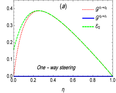
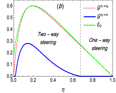
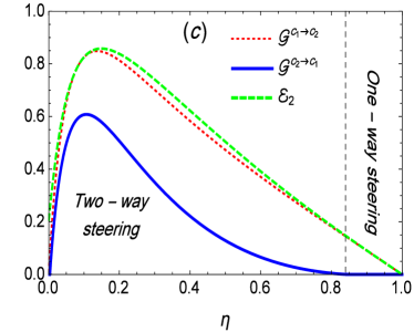
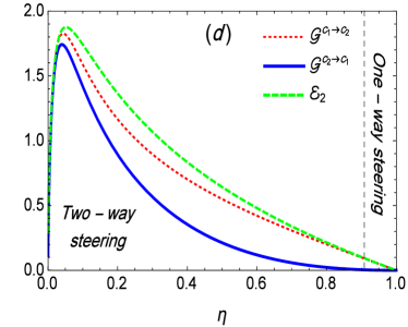
Figure 2: The Gaussian steering $\mathcal{G}^{c_{1}\rightarrow c_{2}}$, $\mathcal{G}^{c_{2}\rightarrow c_{1}}$ and the Gaussian Rényi-2 entanglement $\mathcal{E}_{2}$ as functions of the population inversion $\eta$ using various values of the linear gain coefficient: (a) $A=50~{}\text{kHz}$, (b) $A=100~{}\text{kHz}$, (c) $A=200~{}\text{kHz}$, and (d) $A=2000~{}\text{kHz}$. The cavity decay rate is fixed as $\kappa=3.85~{}\text{kHz}$. Panel (a) shows an interesting situation in which the state $\hat{\varrho}_{c_{1}c_{2}}$ is entangled, however, it is steerable only from $c_{1}\rightarrow c_{2}$, which clearly reflects the asymmetric property of quantum correlations. Quite remarkably, panel (d) shows that maximum steering and entanglement can be achieved by inducing maximum quantum coherence in the cavity, which corresponds to $\eta\rightarrow 0$ and $A\gg 1$.

For realistic estimation of both steering and entanglement of the two laser modes $c_{1}$ and $c_{2}$, we use experimental parameters from [36, 55]: the cavity decay rate for the laser modes c₁ and c₂ is $\kappa=3.85~{}\text{kHz}$, the atomic damping rate $\gamma=20~{}\text{kHz}$, the atomic coupling strength $\epsilon=43~{}\text{kHz,}$ and $\rho=22~{}\text{kHz}$ as value of the rate at which the atoms are initially injected into the cavity. Using these parameters, one has $A=2\rho\epsilon^{2}/\gamma^{2}\approx 200~{}\text{kHz}$ for the linear gain coefficient.

In Fig. 2, we plot the steerabilities $\mathcal{G}^{c_{1}\rightarrow c_{2}}$ and $\mathcal{G}^{c_{2}\rightarrow c_{1}}$ as well as the Gaussian Rényi-2 entanglement $\mathcal{E}_{2}$ as functions of the population inversion $\eta$ using various values of the linear gain coefficient $A$. First, we remark that the steering and entanglement behave similarly under the same circumstances. In addition, the values of the steering $\mathcal{G}^{c_{1}\rightarrow c_{2}}$ are fully differ from those of the steering in the reverse direction $\mathcal{G}^{c_{2}\rightarrow c_{1}}$, which clearly reflects the role of the measurement in quantum mechanics. Interestingly, Fig. 2 shows that for $\eta=1$, the steering in both directions $c_{1}\rightleftarrows c_{2}$ as well as the entanglement $\mathcal{E}_{2}$ vanish regardless of the choice of the linear gain coefficient $A$. These results can be explained as follows: since $\eta=1$ corresponds to the case in which all the atoms are initially prepared in the lower energy level $|l\rangle$, then no possibility for radiation emission by the atoms in this case, and further no quantum correlations (including steering and entanglement) can be generated between the modes $c_{1}$ and $c_{2}$. Besides, when $\eta\rightarrow 0$, which corresponds to the situation in which the atoms are initially prepared with maximum quantum coherence, we remark that maximum steering and entanglement could be achieved. Strikingly, Fig. 2(a) shows that the state $\hat{\varrho}_{c_{1}c_{2}}$ is steerable only from $c_{1}\rightarrow c_{2}$ (one-way steering), although the two modes $c_{1}$ and $c_{2}$ are entangled. This could be explained as follows: Alice (owning the mode $c_{1}$) and Bob (owning the mode $c_{2}$) can implement the same Gaussian measurements on their shared entangled state $\hat{\varrho}_{c_{1}c_{2}}$, however obtain different results, which reflects the asymmetric property of quantum correlations. In other words, one-way steering from $c_{1}\rightarrow c_{2}$ means that Alice can convince Bob that their shared state is entangled, in contrast, the reverse process is impossible. This is partly due to the asymmetric form of the covariance matrix (16), wherein $\sigma_{1}\neq\sigma_{2}$, and partly due to the definition of the steerabilities $\mathcal{G}^{c_{1}\rightarrow c_{2}}$ and $\mathcal{G}^{c_{2}\rightarrow c_{1}}$.

In particular, Figs. 2(b), 2(c) and 2(d) show that by using high values of the linear gain coefficient $A$, two-way steering can be observed, and further it can be transformed into one-way steering when $\eta\rightarrow 1.$

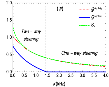
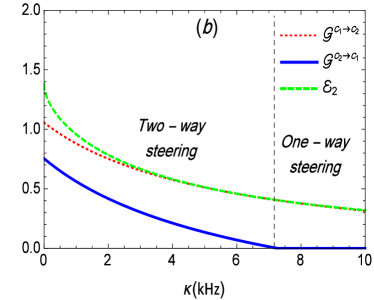
Figure 3: The Gaussian steering $\mathcal{G}^{c_{1}\rightarrow c_{2}}$, $\mathcal{G}^{c_{2}\rightarrow c_{1}}$ and the Gaussian Rényi-2 entanglement $\mathcal{E}_{2}$ against the cavity decay rate $\kappa$ using two different values of the linear gain coefficient: (a) $A=20~{}\text{kHz}$, and (b) $A=100~{}\text{kHz}$. The population inversion is fixed as $\eta=0.25$. As expected, both steering and entanglement decay under the cavity losses, and they can be enhanced by augmenting the coefficient $A$, i.e., the rate at which the atoms are injected into the cavity. Similarly to Fig. 2, Fig. 3 shows that one-way steering still occurs only from $c_{1}\rightarrow c_{2}$ and the steering $\mathcal{G}^{c_{1}\rightarrow c_{2}}$ and $\mathcal{G}^{c_{2}\rightarrow c_{1}}$ remain less than entanglement $\mathcal{E}_{2}$.

On the other hand, Fig. 3 illustrates the dependence of the steering $\mathcal{G}^{c_{1}\rightarrow c_{2}}$ and $\mathcal{G}^{c_{2}\rightarrow c_{1}}$ and the Gaussian Rényi-2 entanglement $\mathcal{E}_{2}$ on the cavity decay rate $\kappa$ using $A=20~{}$kHz in panel (a), and $A=100~{}$kHz in panel (b). The population inversion is fixed as $\eta=0.25$. As shown, $\mathcal{G}^{c_{1}\rightarrow c_{2}}$, $\mathcal{G}^{c_{2}\rightarrow c_{1}}$ and $\mathcal{E}_{2}$ are maximum for $\kappa=0$, and have a tendency to diminish with increasing dissipation $\kappa$. Similarly to the results presented in Fig. 2, Fig. 3 shows that one-way steering still occurs only from $c_{1}\rightarrow c_{2}$, which emerges from the fact that the steering $\mathcal{G}^{c_{1}\rightarrow c_{2}}$ remains greater than the steering $\mathcal{G}^{c_{2}\rightarrow c_{1}}$. Importantly, Figs. 2 and 3 show together that the range of one-way steering is strongly influenced by the values of linear gain coefficient $A$. Additionally, they show that the steering $\mathcal{G}^{c_{1}\rightarrow c_{2}}$ and $\mathcal{G}^{c_{2}\rightarrow c_{1}}$ are upper bounded by the Gaussian Rényi-2 entanglement $\mathcal{E}_{2}$, which is well supported by the results illustrated in Fig. 4. Indeed, with density values of the physical parameters $A$, $\kappa$ and $\eta$ of the state $\hat{\varrho}_{c_{1}c_{2}}$, Fig. 4 shows that the difference $\mathcal{E}_{2}-\mathcal{G}^{\leftrightarrow}$, where $\mathcal{G}^{\leftrightarrow}=\mathrm{Max[\mathcal{G}^{c_{1}\rightarrow c_{2}},\mathcal{G}^{c_{2}\rightarrow c_{1}}]}$ [8], remains always positive or equal to zero, meaning that the maximum steering $\mathcal{G}^{\leftrightarrow}$ cannot exceed the Gaussian Rényi-2 entanglement $\mathcal{E}_{2}$ of the two laser modes $c_{1}$ and $c_{2}$. This therefore is consistent with the Ref. [8].

Quite remarkably, Figs. 2 and 3 show that one-way steering is occurred—within various circumstances—only in the direction $c_{1}\rightarrow c_{2}$. In what follows, we demonstrate that—in general—the state $\hat{\varrho}_{c_{1}c_{2}}$ can exhibit one-way steering behavior only from $c_{1}\rightarrow c_{2}$.

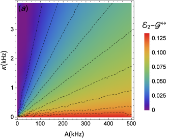
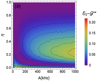
Figure 4: (a) Density plot of the difference $\mathcal{E}_{2}-\mathcal{G}^{\leftrightarrow}$ (with $\mathcal{G}^{\leftrightarrow}=\text{Max}[\mathcal{G}^{c_{1}\rightarrow c_{2}}$, $\mathcal{G}^{c_{2}\rightarrow c_{1}}]$) versus $\kappa$ and $A$ using $\eta=0.5$. (b) Density plot of $\mathcal{E}_{2}-\mathcal{G}^{\leftrightarrow}$ versus $\eta$ and $A$ using $\kappa=3.85~{}\text{kHz}$. In various circumstances, we remark that the Gaussian Rényi-2 entanglement $\mathcal{E}_{2}$ is always greater or equal to the maximum steering $\mathcal{G}^{\leftrightarrow}$, which is consistent with the Ref. [8].

Indeed, since $\mathcal{G}^{c_{1}\rightarrow c_{2}}\geqslant\mathcal{G}^{c_{2}\rightarrow c_{1}}$ (which includes $\mathcal{G}^{c_{1}\rightarrow c_{2}}>0$ and $\mathcal{G}^{c_{2}\rightarrow c_{1}}=0$) is a necessary condition for observing one-way steering from $c_{1}\rightarrow c_{2}$, hence, the general fulfilling of the constraint $\mathcal{G}^{c_{1}\rightarrow c_{2}}\geqslant\mathcal{G}^{c_{2}\rightarrow c_{1}}$ implies that one-way steering can occur only from $c_{1}\rightarrow c_{2}$. Then, utilizing Eqs. (16) and (19), one can show that $\mathcal{G}^{c_{1}\rightarrow c_{2}}\geqslant\mathcal{G}^{c_{2}\rightarrow c_{1}}$ is equivalent to $\langle\hat{c}_{1}^{{\dagger}}\hat{c}_{1}\rangle_{ss}\geqslant\langle\hat{c}_{2}^{{\dagger}}\hat{c}_{2}\rangle_{ss}$, where $\langle\hat{c}_{1}^{{\dagger}}\hat{c}_{1}\rangle_{ss}$($\langle\hat{c}_{2}^{{\dagger}}\hat{c}_{2}\rangle_{ss}$) is the mean photon number in the laser mode $c_{1}$($c_{2}$). Moreover, employing Eqs. (13) and (14), we obtain $\langle\hat{c}_{1}^{{\dagger}}\hat{c}_{1}\rangle_{ss}-\langle\hat{c}_{2}^{{\dagger}}\hat{c}_{2}\rangle_{ss}=\frac{A\left(1-\eta\right)}{2\left(\kappa+A\eta\right)}$, which is always positive because $0\leqslant\eta\leqslant 1$, $A\geqslant 0$, and $\kappa\geqslant 0$. This means that the condition $\mathcal{G}^{c_{1}\rightarrow c_{2}}\geqslant\mathcal{G}^{c_{2}\rightarrow c_{1}}$ is always satisfied. Therefore, one-way steering can occur between the modes $c_{1}$ and $c_{2}$ only in the direction $c_{1}\rightarrow c_{2}$. The demonstrated unidirectional one-way steering may lead to more consideration in the application of asymmetric quantum steering [16].

Finally, with the availability of cavity-quantum electrodynamics and trapped atoms techniques [56, 57], and the homodyne detection method developed in [34], these results may be verified experimentally.

4 Conclusion

In a two-mode Gaussian state $\hat{\varrho}_{c_{1}c_{2}}$, asymmetric quantum steering is studied. The modes $c_{1}$ and $c_{2}$ are generated, respectively, during the first and second transition of a nondegenerate three-level laser. By means of the master equation that governs the dynamics of the state $\hat{\varrho}_{c_{1}c_{2}}$, we derived analytical expression of the stationary covariance matrix describing any Gaussian state of the two laser modes $c_{1}$ and $c_{2}$ . To quantify the amount by which the state $\hat{\varrho}_{c_{1}c_{2}}$ is steerable in a given direction, we employed the measure proposed in [8]. Using realistic experimental parameters, we showed that it is possible to generate stationary Gaussian steering in both directions $c_{1}\rightleftarrows c_{2}$ (two-way steering), and even one-way steering. Also, we showed that by an appropriate choice of the physical parameters of the state $\hat{\varrho}_{c_{1}c_{2}}$ (quantum coherence and cavity decay rate), the region of one-way steering can be controlled, which may have potential applications in asymmetric quantum information tasks [16]. Importantly, we demonstrated that in the considered state $\hat{\varrho}_{c_{1}c_{2}}$: (i) the $c_{2}\rightarrow c_{1}$ steerability cannot exceed that in the reverse direction, (ii) one-way steering can, in general, occur only from $c_{1}\rightarrow c_{2}.$ On the other hand, we compared the Gaussian steering of the two laser modes $c_{1}$ and $c_{2}$ with their corresponding entanglement quantified by means of the Gaussian Rényi-2 entanglement. These two kind of quantum correlations (steering and entanglement) are found to behave similarly under the same circumstances, i.e., they are found to decay under influence of the cavity losses, while they could be well enhanced by inducing more and more quantum coherence into the cavity. In particular, it is found that the steering remains upper bounded by the Gaussian Rényi-2 entanglement. With these results, we believe that nondegenerate three-level laser systems may have immediate applications in the implementing of asymmetric quantum information processing and communication.

References

- [1] E. Schrödinger, Proc. Cambridge Philos. Soc. 31, 555 (1935).
- [2] E. Schrödinger, Proc. Cambridge Philos. Soc. 32, 446 (1936).
- [3] A. Einstein, B. Podolsky and N. Rosen, Phys. Rev. 47, 777 (1935).
- [4] H. M. Wiseman, S. J. Jones and A. C. Doherty, Phys. Rev. Lett. 98, 140402 (2007).
- [5] R. Horodecki, P. Horodecki, M. Horodecki and K. Horodecki, Rev. Mod. Phys. 81, 865 (2009).
- [6] J. S. Bell, Physics 1, 195 (1964).
- [7] M. A. Nielsen and I. L. Chuang, Quantum Computation and Quantum Information (Cambridge University Press, Cambridge, 2000).
- [8] I. Kogias, A. R. Lee, S. Ragy and G. Adesso, Phys. Rev. Lett. 114, 060403 (2015).
- [9] M. D. Reid, Phys. Rev. A 40, 913 (1989).
- [10] E. G. Cavalcanti, S. J. Jones, H. M. Wiseman and M. D. Reid, Phys. Rev. A 80, 032112 (2009).
- [11] A.C.S. Costa, R. Uola and O. Gühne, Phys. Rev. A 98, 050104(R) (2018).
- [12] S.P. Walborn, A. Salles, R.M. Gomes, F. Toscano and P.H. Souto Ribeiro, Phys. Rev. Lett. 106, 130402 (2011).
- [13] C. Weedbrook, S. Pirandola, R. G. -Patrón, N. J. Cerf, T. C. Ralph, J. H. Shapiro and S. Lloyd, Rev. Mod. Phys. 84, 621 (2012).
- [14] A. Rényi, in Proceedings of the 4th Berkeley Symposium on Mathematics, Statistics and Probability: held at the Statistical Laboratory, University of California, 1960, edited by J. Neyman (University of California Press, Berkeley, 1961), pp.547–561.
- [15] G Adesso, D Girolami and A Serafini, Phys. Rev. Lett. 109, 190502 (2012).
- [16] R. Uola, A. C. S. Costa, H. C. Nguyen and O. Gühne, Rev. Mod. Phys. 92, 015001 (2020).
- [17] N. Walk, S. Hosseini, J. Geng, O. Thearle, J. Y. Haw, S. Arm strong, S. M. Assad, J. Janousek, T. C. Ralph, T. Symul, H. M. Wiseman and P. K. Lam, Optica 3, 634 (2016).
- [18] I. Kogias, Y. Xiang, Q. He and G. Adesso, Phys. Rev. A 95, 012315 (2017).
- [19] Q. Y. He, L. Rosales-Zárate, G. Adesso and M. D. Reid, Phys. Rev. Lett. 115, 180502 (2015).
- [20] C. M. Li, K. Chen, Y. N. Chen, Q. Zhang, Y. A. Chen and J. W. Pan, Phys. Rev. Lett. 115, 010402 (2015).
- [21] M. Piani and J. Watrous, Phys. Rev. Lett. 114, 060404 (2015).
- [22] H. Tan,1, W. Deng, Q. Wu and G. Li, Phys. Rev. A 95, 053842 (2017).
- [23] H. Tan, X. Zhang and G. Li, Phys. Rev. A 91, 032121 (2015).
- [24] Q. Y. He and M. D. Reid, Phys. Rev. A 88, 052121 (2013).
- [25] W. Zhong, D. Zhao, G. Cheng and A. Chen, Opt. Commun. 497, 127138 (2021).
- [26] D. Kong, J. Xu, Y. Tian, F. Wang and X. Hu, Phys. Rev. Research, 4, 013084 (2022).
- [27] Z-B. Yang, X-D. Liu, X-Y. Yin, Y. Ming, H-Y. Liu and R-C. Yang, Phys. Rev. Appl. 15, 024042 (2021).
- [28] X. Deng, Yu Xiang, C. Tian, G. Adesso, Q. He, Q. Gong, X. Su, C. Xie and K. Peng, Phys. Rev. Lett. 118, 230501 (2017).
- [29] J. Wang, H. Cao, J. Jing and H. Fan, Phys. Rev. D 93, 125011 (2016).
- [30] S. L. W. Midgley, A. J. Ferris and M. K. Olsen, Phys. Rev. A 81, 022101 (2010).
- [31] F. Ming, X.-K. Song, J. Ling, L. Ye and D. Wang, Eur. Phys. J. C 80, 275 (2020).
- [32] S. Ullah, H. S. Qureshi and F. Ghafoor, Opt. Express 27, 26873 (2019).
- [33] W. Zhong, G. Cheng and X. Hu, Laser Phys. Lett. 17, 125201 (2019).
- [34] J. Laurat, G. Keller, J. A. Oliveira-Huguenin, C. Fabre, T. Coudreau, A. Serafini, G. Adesso and F. Illuminati, J. Opt. B: Quantum Semiclass. Opt. 7, S577 (2005).
- [35] M. O. Scully and M. S. Zubairy, Quantum Optics (Cambridge University Press, Cambridge, 1997).
- [36] H. Xiong, M. O. Scully and M. S. Zubairy, Phys. Rev. Lett. 94, 023601 (2005).
- [37] E. A. Sete and H. Eleuch, J. Opt. Soc. Am. B 32, 971 (2015).
- [38] E. Alebachew and K. Fesseha, Opt. Commun. 265, 314 (2006).
- [39] K. Fesseha, Phys. Rev. A 63, 033811 (2001).
- [40] S. Tesfa, Phys. Rev. A 74, 043816 (2006).
- [41] M. O. Scully, K. Wódkiewicz, M. S. Zubairy, J. Bergou, N. Lu and J. Meyer ter Vehn, Phys. Rev. Lett. 60, 1832 (1988).
- [42] N. A. Ansari, Phys. Rev. A 48, 4686 (1993).
- [43] N. Lu, F. X. Zhao and J. Bergou, Phys. Rev. A 39, 5189 (1989).
- [44] E. Alebachew, Phys. Rev. A 76, 023808 (2007).
- [45] C. A. Blockley and D.F. Walls, Phys. Rev. A 43, 5049 (1991).
- [46] M. H. Louisell, Quantum Statistical Properties of Radiation (Wiley, New York, 1973).
- [47] O. El Akramine, A. Makhoute, M. Zitane and M. Tij, Phys. Rev. A 58, 4892 (1988).
- [48] M. Sargent III, M. O. Scully and W. E. Lamb Jr., Laser physics (Addison-Wesley, Reading, Mass., 1974).
- [49] J. E Qars, Ann. Phys. (Berlin) 534(6), 2100386 (2022).
- [50] J. E Qars, Commun. Theor. Phys. 73(5), 055103 (2021).
- [51] S. Tesfa, Phys. Rev. A 79, 033810 (2009).
- [52] H.- T. Tan, S-.Y. Zhu and M. S. Zubairy, Phys. Rev. A 72, 022305 (2005).
- [53] G. Adesso and F. Illuminati, Phys. Rev. A 72, 032334 (2005).
- [54] G. Adesso and A. Datta, Phys. Rev. Lett. 105, 030501 (2010).
- [55] D. Meschede, H. Walther and G. Muller, Phys. Rev. Lett. 54, 551 (1985).
- [56] A. Reiserer and G. Rempe, Rev. Mod. Phys. 87, 1379 (2015).
- [57] J. McKeever, A. Boca, A. D. Boozer, R. Miller, J. R. Buck, A. Kuzmich and H. J. Kimble, Science, 303, 1992 (2004).