Quantum steering displays an inherent asymmetric property that differs from entanglement and Bell nonlocality. Besides being of fundamental interest, steering is relevant to many asymmetric quantum information tasks. Here, we propose a scheme to generate and manipulate Gaussian quantum steering between two spatially distant mechanical modes of two optomechanical cavities coupled via an optical fiber, and driven by blue detuned lasers. In the unresolved sideband regime, we show, under realistic experimental conditions, that strong asymmetric steering can be generated between the two considered modes. Also, we show that one-way steering can be achieved and practically manipulated through the lasers drive powers and the temperatures of the cavities. Further, we reveal that the direction of one-way steering depends on the sign of the difference between the energies of the mechanical modes. Finally, we discuss how to access the generated steering. This work opens up new perspectives for the distribution of long-distance trust which is of great interest in secure quantum communication.

1 Introduction

In their seminal paper 1935 [1], Einstein, Podolski, and Rosen (EPR) have considered two particles in a pure entangled state to illustrate why they questioned the incompatibility between the concept of local causality and the completeness of quantum mechanics. In fact, they pointed out that a measurement performed on one particle induces an apparent nonlocal collapse of the quantum state of the other, which was unacceptable for them. The EPR paradox provoked an interesting analysis from Schrödinger [2, 3], who introduced the aspect of steering to describe the spooky action-at-a-distance discussed by EPR.

Within mixed states, quantum nonlocality can arise in various incarnations, i.e., Bell nonlocality [4], quantum steering [5], and entanglement [6]. In terms of violations of local hidden state model, EPR steering was defined by Wiseman and co-workers [7] as a form of quantum correlations that sets between Bell nonlocality [4] and entanglement [6], and which allows one observer to remotely affect (steer) the state of another distant observer via local measurements [8]. Importantly, Wiseman et al. [7] showed the hierarchy of the three kind of quantum nonlocal states, that is, steerable states are a subset of the entangled states and a superset of Bell nonlocal states [7]. Put in other word, a bipartite state $\hat{\varrho}_{xy}$ that displays Bell nonlocality is steerable in both directions $x\rightleftarrows y$, whereas, EPR steering at least in one direction implies that the state is entangled [5]. The reverse scenario is not always true, meaning that not all entangled states are steerable, and not every steerable state exhibits Bell nonlocality [9].

From a quantum information perspective [5], quantum steering corresponds to the task of verifiable entanglement distribution by an untrusted party, i.e., if Alice and Bob share a quantum bipartite state which is steerable, say, from Alice to Bob, therefore, Alice can convince Bob, who does not trust her, that the shared state is entangled through local measurements and classical communication.

On the basis of the inferred quadrature variances of light fields, Reid proposed practical criteria for witnessing the existence of the EPR paradox [10], which were experimentally violated in [11, 12, 13]. Especially, it has been proven that violation of the Reid criteria, under Gaussian measurements, demonstrates EPR steering [7]. Later, various criteria which are explicitly concerned with EPR steering were proposed [14], where each criterion depends on the size of the studied system and the detection method [15].

Besides, the quantification of EPR steering has attracted considerable attention in the past decade, which results in miscellaneous useful measures, e.g., steering weight [16] and steering robustness [17], where both measures can be evaluated only by means of a semidefinite program [9]. Within the Gaussian framework [18], Kogias et al. [19] introduced a computable measure of steering for arbitrary bipartite Gaussian states. Essentially, they provided an operational connection between the proposed measure and the key rate in one-sided device-independent quantum key distribution (1SDI-QKD) [20].

Unlike entanglement and Bell nonlocality, EPR steering is intrinsically asymmetric, i.e., a bipartite state $\hat{\varrho}_{xy}$ may be steerable from $x\rightarrow y$, but not vice versa. Thus, one distinguishes, (i) no-way steering where the state $\hat{\varrho}_{xy}$ is nonsteerable neither from $x\rightarrow y$ nor in the reverse direction, (ii) two-way steering where $\hat{\varrho}_{xy}$ is steerable in both directions $x\rightleftarrows y$, and (iii) one-way steering, in which the steerability is authorized solely from $x\rightarrow y$ or $y\rightarrow x$. It is now believed that the key ingredient of asymmetric quantum information tasks is EPR steering [5], which has been recognized as the essential resource for 1SDI-QKD [20], secure quantum teleportation [21, 22, 23], subchannel discrimination [17], quantum secret sharing [24], randomness generation [25], and secure quantum communication [26, 27].

EPR steering has been investigated theoretically as well as experimentally in various continuous-variable systems. Proposals include, cavity magnomechanical systems [28], Gaussian cluster states [29], optical systems [30], and nondegenerate three level laser system [31]. In particular, based on cavity optomechanics [32], a number of schemes for EPR steering generation were proposed in various two-mode Gaussian states [33, 34, 35, 36, 37, 38, 39]. These, however, cannot be used to implement long-distance secure quantum communication, since the two considered modes belong to the same cavity.

The aim of this paper is to investigate, using experimentally feasible parameters, the generation and manipulation of stationary Gaussian EPR steering between two mechanical modes of two spatially separated Fabry-Pérot cavities coupled by an optical fiber. Our work goes beyond the proposals put forward in Refs. [40, 41], where an additional squeezed light source to drive the two cavities was considered.

Optomechanics involves hybrid coupling between optical and mechanical degrees of freedom by means of radiation pressure [32]. Over the last few years, cavity optomechanics has emerged as a very promising platform for demonstrating various quantum features. The important achievements in this realm encompass preparing entangled states between photons and phonons [42, 43], cooling the fundamental vibrational mode to the ground state [44], creation of macroscopic Schrödinger’s cat’ states [45], observing the radiation pressure shot-noise [46], and squeezing effect [47].

The remainder of this paper is organized as follows. In Sec. 2, we introduce the basic optomechanical setup at hand. Next, using the standard Langevin formalism, we derive the covariance matrix describing the whole system at the steady state. In Sec. 3, we quantify and study Gaussian quantum steering between two spatially separated mechanical modes. Also, we discuss how the generated mechanical steering can be experimentally measured. In Sec. 4, we discuss a way to access experimentally the generated optomechanical steering. Finally, in Sec. 5 we draw our conclusions.

2 The system and its covariance matrix

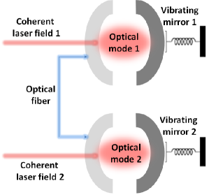
Figure 1: Schematic illustration of two spatially separated Fabry-Pérot cavities coupled to each other by an optical fiber, and driven by two coherent lasers fields. As a consequence of indirect coupling mediated by the two optical modes, the two vibrating mirrors become quantumly correlated.

In Fig. 1, we consider a double-cavity optomechanical system, where each cavity comprises two mirrors. The first one is fixed and partially transmitting, while the second is movable and perfectly reflective. The $j\mathrm{th}$ cavity, having equilibrium length $\ell_{j}$ and decay rate $\kappa_{j}$, is driven by a coherent laser field of power ${\wp}_{j}$ and frequency $\omega_{L_{j}}$. In a frame rotating with the frequency $\omega_{L_{j}}$, the system can be described by the Hamiltonian [48]

$$\mathcal{\hat{H}}=\sum_{j=1}^{2}\Big{(}\hbar\left(\omega_{c_{j}}-\omega_{L_{j}}\right)\hat{o}_{j}^{{\dagger}}\hat{o}_{j}+\frac{\hbar\omega_{m_{j}}}{2}(\hat{q}_{j}+\hat{p}_{j})-\hbar g_{j}\hat{o}_{j}^{{\dagger}}\hat{o}_{j}\hat{q}_{j}+\mathrm{i}\hbar\mathcal{E}_{j}(\hat{o}_{j}^{{\dagger}}-\hat{o}_{j})+\hbar\zeta\hat{o}_{j}^{{\dagger}}\hat{o}_{3-j}\Big{)},$$ (1)

where the first term describes the free Hamiltonian of the $j\mathrm{th}$ intracavity laser field modeled as a single optical mode with annihilation operator $\hat{o}_{j}$ and frequency $\omega_{c_{j}}$. The second term describes the free Hamiltonian of the $j\mathrm{th}$ movable mirror modeled as a single mechanical mode with position-$\hat{q}_{j}$ and momentum-$\hat{p}_{j}$ operators, an effective mass $\mu_{j}$, frequency $\omega_{m_{j}}$, and damping rate $\gamma_{j}$. The third term comes from the optomechanical coupling, via the radiation pressure force, between the $j\mathrm{th}$ mechanical mode and the $j\mathrm{th}$ optical mode, with $g_{{}_{j}}=\frac{\omega_{c_{j}}}{\ell_{j}}\sqrt{\frac{\hbar}{\mu_{{}_{j}}\omega_{m_{j}}}}$. The fourth term describes the coupling between the $j\mathrm{th}$ input laser and the $j\mathrm{th}$ optical mode, with $\mathcal{E}_{j}=\sqrt{\frac{2\kappa_{j}{\wp}_{j}}{\hbar\omega_{L_{j}}}}$. The last term corresponds to the coupling between the two optical modes $\hat{o}_{1}$ and $\hat{o}_{2}$, with coupling strength $\zeta$.

Since the system at hand is affected by dissipation and noise, then its dynamics can be described by the following quantum Langevin equation [49], i.e., $\frac{d\mathcal{\hat{O}}}{dt}=\frac{1}{\mathrm{i}\hbar}\left[\mathcal{\hat{O}},\mathcal{\hat{H}}\right]+$$\mathcal{\hat{D}}+\mathcal{\hat{N}}$ (for $\mathcal{\hat{O}\equiv}\hat{o}_{j},\hat{q}_{j}$, $\hat{p}_{j}$), where $\mathcal{\hat{D}}$ and $\mathcal{\hat{N}}$ characterize the dissipation and noise, respectively. For the Hamiltonian (1), we obtain

$$\frac{d\hat{o}_{j}}{dt} = -\left(\kappa_{j}+i\Delta_{0_{j}}\right)\hat{o}_{j}+\mathrm{i}g_{j}\hat{o}_{j}\hat{q}_{j}-\mathrm{i}\zeta\hat{o}_{3-j}+\mathcal{E}_{j}+\sqrt{2\kappa_{j}}\hat{o}_{j}^{in},$$ (2)

$$\frac{d\hat{q}_{j}}{dt} = \omega_{m_{j}}\hat{p}_{j},$$ (3)

$$\frac{d\hat{p}_{j}}{dt} = -\omega_{m_{j}}\hat{q}_{j}+g_{j}\hat{o}_{j}^{{\dagger}}\hat{o}_{j}-\gamma_{j}\hat{p}_{j}+\hat{\xi}_{j},$$ (4)

where $\Delta_{0_{j}}=\omega_{c_{j}}-\omega_{L_{j}}$ is the $j\mathrm{th}$ laser detuning [49]. In Eq. (2), $\hat{o}_{j}^{in}$ denotes the $j\mathrm{th}$ zero mean vacuum radiation input noise with the correlation function $\langle\hat{o}_{j}^{in}(t)\hat{o}_{j}^{in{\dagger}}(t^{\prime})\rangle=\delta(t-t^{\prime})$ [50]. While, in Eq. (4) $\hat{\xi}_{j}$ is the zero-mean Brownian noise operator affecting the $j\mathrm{th}$ mechanical mode. It turns out that quantum effects can be reached only by using mechanical oscillators with high mechanical quality factor $Q_{j}=\omega_{m_{j}}/\gamma_{j}\gg 1$ [32]. In this limit, we have the following nonzero correlation function [51]

$$\langle\hat{\xi}_{j}(t)\hat{\xi}_{j}(t^{\prime})+\hat{\xi}_{j}(t^{\prime})\hat{\xi}_{j}(t)\rangle/2=\gamma_{j}(2n_{\mathrm{th},j}+1)\delta(t-t^{\prime}),$$ (5)

where $n_{\mathrm{th},j}=(e^{\hbar\omega_{m_{j}}/k_{B}T_{j}}-1)^{-1}$ is the $j\mathrm{th}$ mean thermal phonon number. $T_{j}$ and $k_{B}$ are the $j\mathrm{th}$ mirror temperature and the Boltzmann constant, respectively.

Due to the nonlinearity of Eq. (1), the coupled quantum Langevin equations [(2)-(4)] are not in general solvable analytically. However, using bright inputs lasers, the linearization of these equations around the steady-state values is justified, and the dynamics can be solved exactly. Hence, by adopting the standard linearization method [50], we decompose each operator ($\mathcal{\hat{O}\equiv}\hat{o}_{j},\hat{q}_{j}$, $\hat{p}_{j}$) as a sum of the steady-state value $\langle\mathcal{\hat{O}\rangle}$ and a fluctuation operator $\delta\mathcal{\hat{O}}$ with zero mean value, i.e., $\mathcal{\hat{O}=}$ $\langle\mathcal{\hat{O}\rangle+}\delta\mathcal{\hat{O}}$. By setting $\frac{d}{dt}=0$ in Eqs. [(2)-(4)] and solving the obtained equations, we get $\langle\hat{q}_{j}\rangle=\frac{g_{j}\left|\langle\hat{o}_{j}\rangle\right|^{2}}{\omega_{m_{j}}}$, $\langle\hat{p}_{j}\rangle=0$, and $\langle\hat{o}_{j}\rangle=\frac{\mathcal{E}_{j}\left[\kappa_{j}+\mathrm{i}\left(-\zeta+\Delta_{3-j}\right)\right]}{\zeta^{2}+\kappa_{j}^{2}-\Delta_{1}\Delta_{2}+\mathrm{i}\kappa_{j}(\Delta_{1}+\Delta_{2})}$, with $\Delta_{j}$ $=$ $\Delta_{0_{j}}$ $-g_{j}\langle\hat{q}_{j}\rangle$ being the $j\mathrm{th}$ effective cavity detuning [49]. Now, by inserting $\mathcal{\hat{O}=}$ $\langle\mathcal{\hat{O}\rangle+}\delta\mathcal{\hat{O}}$ into Eqs. [(2)-(4)], and assuming that the two cavities are intensely driven, i.e., $\left|\langle\hat{o}_{j}\rangle\right|\gg 1$, which allows us to safely neglect the quadratic terms $\delta\hat{o}_{j}^{{\dagger}}\delta\hat{o}_{j}$ and $\delta\hat{o}_{j}\delta\hat{q}_{j}$, we obtain

$$\frac{d\delta\hat{o}_{j}}{dt} = -\left(\kappa_{j}+\mathrm{i}\Delta_{j}\right)\delta\hat{o}_{j}+\mathrm{i}g_{j}\langle\hat{o}_{j}\rangle\delta\hat{q}_{j}-\mathrm{i}\zeta\delta\hat{o}_{3-j}+\sqrt{2\kappa_{j}}\hat{o}_{j}^{in},$$ (6)

$$\frac{d\delta\hat{q}_{j}}{dt} = \omega_{m_{j}}\delta\hat{p}_{j},$$ (7)

$$\frac{d\delta\hat{p}_{j}}{dt} = -\omega_{m_{j}}\delta\hat{q}_{j}+g_{j}\langle\hat{o}_{j}\rangle\left(\delta\hat{o}_{j}^{{\dagger}}+\delta\hat{o}_{j}\right)-\gamma_{j}\delta\hat{p}_{j}+\hat{\xi}_{j}.$$ (8)

We emphasize that Eq. (8) is obtained under the assumption that the phase reference of the $j\mathrm{th}$ laser field is chosen such that $\langle\hat{o}_{j}\rangle$ is real. Next, introducing the $j\mathrm{th}$ optical mode quadratures $\delta\hat{x}_{j}=(\delta\hat{o}_{j}^{{\dagger}}+\delta\hat{o}_{j})/\sqrt{2}$ and $\delta\hat{y}_{j}=i(\delta\hat{o}_{j}^{{\dagger}}-\delta\hat{o}_{j})/\sqrt{2}$ as well as the $j\mathrm{th}$ input noise quadratures $\delta\hat{x}_{j}^{in}=(\delta\hat{o}_{j}^{in{\dagger}}+\delta\hat{o}_{j}^{in})/\sqrt{2}$ and $\delta\hat{y}_{j}^{in}=i(\delta\hat{o}_{j}^{in{\dagger}}-\delta\hat{o}_{j}^{in})/\sqrt{2}$, and using Eqs. [(6)-(8)], one gets

$$\frac{d\hat{u}(t)}{dt}=\mathcal{K}\hat{u}(t)+\hat{n}(t),$$ (9)

where the transposes of the fluctuations vector $\hat{u}(t)$ and the noises vector $\hat{n}(t)$ are, respectively,

$$\hat{u}(t)^{\mathrm{T}} = \left(\delta\hat{q}_{1}(t),\delta\hat{p}_{1}(t),\delta\hat{q}_{2}(t),\delta\hat{p}_{2}(t),\delta\hat{x}_{1}(t),\delta\hat{y}_{1}(t),\delta\hat{x}_{2}(t),\delta\hat{y}_{2}(t)\right),$$ (10)

$$\hat{n}(t)^{\mathrm{T}} = (0,\hat{\xi}_{1}(t),0,\hat{\xi}_{2}(t),\delta\hat{x}_{1}^{in}(t),\delta\hat{y}_{1}^{in}(t),\delta\hat{x}_{2}^{in}(t),\delta\hat{y}_{2}^{in}(t)),$$ (11)

and the kernel $\mathcal{K}$ is given by

$$\mathcal{K=}\left(\begin{array}[]{cccccccc}0&\omega_{m_{1}}&0&0&0&0&0&0\\ -\omega_{m_{1}}&-\gamma_{1}&0&0&G_{1}&0&0&0\\ 0&0&0&\omega_{m_{2}}&0&0&0&0\\ 0&0&-\omega_{m_{2}}&-\gamma_{2}&0&0&G_{2}&0\\ 0&0&0&0&\kappa_{1}&\Delta_{1}&0&\zeta\\ G_{1}&0&0&0&-\Delta_{1}&\kappa_{1}&-\zeta&0\\ 0&0&0&0&0&\zeta&\kappa_{2}&\Delta_{2}\\ 0&0&G_{2}&0&-\zeta&0&-\Delta_{2}&\kappa_{2}\end{array}\right),$$ (12)

with

$$G_{j}=\sqrt{2}g_{j}\langle\hat{o}_{j}\rangle=\frac{2\omega_{c_{j}}}{\ell_{j}}\sqrt{\frac{\kappa_{j}{\wp}_{j}[\kappa_{j}^{2}+\left(\Delta_{3-j}-\zeta\right)^{2}]}{\mu_{{}_{j}}\omega_{m_{j}}\omega_{L_{j}}[(\zeta^{2}+\kappa_{j}^{2}-\Delta_{1}\Delta_{2})^{2}+\kappa_{j}^{2}(\Delta_{1}+\Delta_{2})^{2}]}},$$ (13)

being the $j\mathrm{th}$ effective coupling [32]. The solution of Eq. (9) writes [43]

$$\hat{u}(t)=f(t)\hat{u}(0)+\int_{0}^{t}dsf(s)\hat{n}(t-s),$$ (14)

with $f(t)=e^{\mathcal{K}t}$. The system under consideration is stable and reaches its steady state when all the eigenvalues of the matrix $\mathcal{K}$ have negative real parts, so that $f(\infty)=0$. The stability conditions can be deduced by applying the Routh-Hurwitz criterion [52]. But in our four-mode Gaussian state case, they are quite involved, and cannot be reported here.

The operators $\hat{o}_{j}^{in}$ and $\hat{\xi}_{j}$ are zero-mean quantum Gaussian noises and the dynamics is linearized. Then, the quantum steady state of the fluctuations is a zero-mean Gaussian state, entirely characterized by its $8\times 8$ covariance matrix $\mathcal{V}_{ii^{\prime}}=(\langle\hat{u}_{i}(\infty)\hat{u}_{i^{\prime}}(\infty)+\hat{u}_{i^{\prime}}(\infty)\hat{u}_{i}(\infty)\rangle)/2$, where $\hat{u}(\infty)$ is the fluctuations vector at the steady state [43]. When the system is stable and using Eq. (14), we obtain

$$\mathcal{V}_{ii^{\prime}}=\sum_{k,k^{\prime}}\int_{0}^{\infty}ds\int_{0}^{\infty}ds^{\prime}f_{{}^{ik}}(s)f_{{}^{i^{\prime}k^{\prime}}}(s^{\prime})\Phi_{{}^{kk^{\prime}}}(s-s^{\prime}),$$ (15)

where $\Phi_{{}^{kk^{\prime}}}(s-s^{\prime})=(\langle\hat{n}_{k}(s)\hat{n}_{k^{\prime}}(s^{\prime})+\hat{n}_{k^{\prime}}(s^{\prime})\hat{n}_{k}(s)\rangle)/2=D_{{}^{kk^{\prime}}}\delta(s-s^{\prime})$ denotes the matrix of stationary noise correlation functions [43]. Using the correlation properties of the operators $\hat{o}_{j}^{in}$ and $\hat{\xi}_{j}$, one can show that $D=D_{\gamma}\oplus D_{\kappa}$, with $D_{\gamma}=\mathrm{diag}\left[0,\gamma_{1}\left(2n_{\mathrm{th,1}}+1\right),0,\gamma_{2}\left(2n_{\mathrm{th,2}}+1\right)\right]$ and $D_{\kappa}=\mathrm{diag}\left[\kappa_{1},\kappa_{1},\kappa_{2},\kappa_{2}\right]$. Hence, Eq. (15) becomes $\mathcal{V}=\int_{0}^{\infty}dsf(s)Df(s)^{\mathrm{T}}$ which is equivalent to the Lyapunov equation [40]

$$\mathcal{KV}+\mathcal{VK}^{\mathrm{T}}=-D.$$ (16)

The mechanical covariance matrix $\mathcal{V}_{m}$ of the two mechanical modes, labelled as $m_{1}$ and $m_{2}$, can be deduced by tracing over the optical elements in the general expression of $\mathcal{V}$. Then, we get

$$\mathcal{V}_{m}=\left(\begin{array}[]{cc}\mathcal{V}_{m_{1}}&\mathcal{V}_{m_{1}/m_{2}}\\ \mathcal{V}_{m_{1}/m_{2}}^{\mathrm{T}}&\mathcal{V}_{m_{2}}\end{array}\right),$$ (17)

where the $2\times 2$ matrices $\mathcal{V}_{m_{1}}$ and $\mathcal{V}_{m_{2}}$ represent, respectively, the first and second mechanical modes, while $\mathcal{V}_{m_{1}/m_{2}}$ describes the correlations between them.

3 Gaussian quantum steering

It has been shown in [7] that a bipartite Gaussian state $\hat{\varrho}_{m_{1}m_{2}}$ with covariance matrix $\mathcal{V}_{m}$ is steerable under Gaussian measurements performed on party $m_{1}$ if, and only if, the inequality $\mathcal{V}_{m}+\mathrm{i}(\Omega_{m_{1}}\oplus\Omega_{m_{2}})\geqslant 0$ is violated, where $\Omega_{m_{1}}=\left(\begin{array}[]{cc}0&0\\ 0&0\end{array}\right)$ and $\Omega_{m_{2}}$ $=\left(\begin{array}[]{cc}0&1\\ -1&0\end{array}\right)$. This constraint yielded Kogias et al. [19] to introduce a computable measure for quantifying the amount by which an arbitrary bipartite Gaussian state $\hat{\varrho}_{m_{1}m_{2}}$ is steerable under Gaussian measurements implemented on party $m_{1}$, i.e.,

$$\mathcal{G}^{m_{1}\rightarrow m_{2}}:=\max\left[0,-\sum\limits_{j:\bar{\nu}_{j}^{m_{2}}<1}\ln\left\{{\bar{\nu}_{j}^{m_{2}}}\right\}\right],$$ (18)

where $\{\bar{\nu}_{j}^{m_{2}}\}$ denotes the symplectic spectra of the Schur complement $\mathcal{V}_{m_{2}}-\mathcal{V}_{m_{1}/m_{2}}^{\mathrm{T}}\mathcal{V}_{m_{1}}^{-1}\mathcal{V}_{m_{1}/m_{2}}$ of $m_{1}$ in the covariance matrix $\mathcal{V}_{m}$ (17). The steering $\mathcal{G}^{m_{1}\rightarrow m_{2}}$ is monotone under Gaussian local operations and classical communication, and it vanishes if the state described by $\mathcal{V}_{m}$ is nonsteerable under Gaussian measurements performed on party $m_{1}$. When $m_{1}$ and $m_{2}$ are two single modes, which we consider in this paper, Eq. (18) acquires the simple form $\mathcal{G}^{m_{1}\rightarrow m_{2}}=\max\left[0,\frac{1}{2}\ln\frac{\det\mathcal{V}_{m_{1}}}{4\det\mathcal{V}_{m}}\right]$ [19]. Similarly, quantum steering in the reverse direction can be obtained by changing the roles of $m_{1}$ and $m_{2}$ in the expression of $\mathcal{G}^{m_{1}\rightarrow m_{2}}$, i.e., $\mathcal{G}^{m_{2}\rightarrow m_{1}}=\max\left[0,\frac{1}{2}\ln\frac{\det\mathcal{V}_{m_{2}}}{4\det\mathcal{V}_{m}}\right]$. A nonzero value of $\mathcal{G}^{m_{1}(m_{2})\rightarrow m_{2}(m_{1})}$ means that the state $\hat{\varrho}_{m_{1}m_{2}}$ is steerable from $m_{1}(m_{2})\rightarrow m_{2}(m_{1})$ under Gaussian measurements performed on mode $m_{1}(m_{2})$.

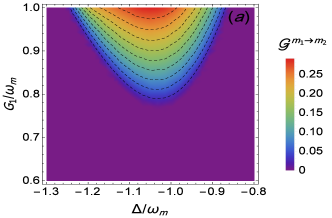
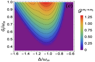
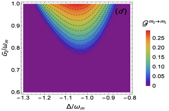
Figure 2: (a) and (b) show, respectively, the steerabilities $\mathcal{G}^{m_{1}\rightarrow m_{2}}$ and $\mathcal{G}^{m_{2}\rightarrow m_{1}}$ versus the normalized detuning $\Delta/\omega_{m}$ and the normalized optomechanical coupling $G_{1}/\omega_{m}$ for $G_{2}=0.5G_{1}$. (c) and (d) show, respectively, $\mathcal{G}^{m_{1}\rightarrow m_{2}}$ and $\mathcal{G}^{m_{2}\rightarrow m_{1}}$ versus $\Delta/\omega_{m}$ and $G_{2}/\omega_{m}$ for $G_{1}=0.5G_{2}$. The other parameters are $\omega_{m}/2\pi=947~{}\mathrm{kHz}$, $\kappa/2\pi=215~{}\mathrm{kHz}$, $\gamma/2\pi=140~{}\mathrm{Hz}$, $\zeta/\omega_{m}=5\times 10^{-2}$, and $n_{\text{th},1}=n_{\text{th},2}=25$.

For achieving asymmetric steering between the two mechanical modes $m_{1}$ and $m_{2}$, we introduce asymmetry between them by imposing $G_{1}\neq G_{2}$. This can be practically realised by choosing identical parameters for the two cavities except the drive lasers powers, i.e., $\wp_{1}\neq\wp_{2}$. Moreover, for realistic estimation of the steerabilities $\mathcal{G}^{m_{1}\rightarrow m_{2}}$ and $\mathcal{G}^{m_{2}\rightarrow m_{1}}$, we use parameters from the experiment [53]. The movable mirrors, having a mass $\mu=145~{}\mathrm{ng}$ and frequency $\omega_{m}=2\pi\times 947~{}\mathrm{kHz}$, are damped at rate $\gamma=2\pi\times 140~{}\mathrm{Hz}$. The two cavities have equilibrium length $\ell=25~{}\mathrm{mm}$, decay rate $\kappa=2\pi\times 215~{}\mathrm{kHz}$, frequency $\omega_{c}=2\pi\times 5.26\times 10^{14}~{}\mathrm{Hz}$, and pumped by lasers of frequency $\omega_{L}=2\pi\times 2.82\times 10^{14}~{}\mathrm{Hz}$.

Figs. 2(a) and 2(b) show, respectively, the steerabilities $\mathcal{G}^{m_{1}\rightarrow m_{2}}$ and $\mathcal{G}^{m_{2}\rightarrow m_{1}}$ versus the normalized detuning $\Delta/\omega_{m}$ and the normalized optomechanical coupling strength $G_{1}/\omega_{m}$ using $G_{2}=0.5G_{1}$. While, Figs. 2(c) and 2(d) show, respectively, $\mathcal{G}^{m_{1}\rightarrow m_{2}}$ and $\mathcal{G}^{m_{2}\rightarrow m_{1}}$ versus $\Delta/\omega_{m}$ and $G_{2}/\omega_{m}$ using $G_{1}=0.5G_{2}$. In the four cases, we used $n_{\text{th},1}=n_{\text{th},2}=25$ and $\zeta/\omega_{m}=5\times 10^{-2}$. As shown, without external lasers, i.e., $\wp_{j}=0$, which, following Eq. (13), is equivalent to $G_{j}=0$, no steering can be created between the modes $m_{1}$ and $m_{2}$ in both directions, namely $\mathcal{G}^{m_{1}\rightarrow m_{2}}=\mathcal{G}^{m_{2}\rightarrow m_{1}}=0$. Besides, by increasing gradually the drive lasers powers $\wp_{1}$ and $\wp_{2}$, which in turn enhances the optomechanical coupling strengths $G_{1}$ and $G_{2}$, the steerabilities $\mathcal{G}^{m_{1}\rightarrow m_{2}}$ and $\mathcal{G}^{m_{2}\rightarrow m_{1}}$ appear and grow monotonously, reaching their maximum around $\Delta/\omega_{m}\approx-1$ for $G_{1}/\omega_{m}\approx 1$ in [Figs. 2(a) and 2(b)], and for $G_{2}/\omega_{m}\approx 1$ in [Figs. 2(c) and 2(d)].

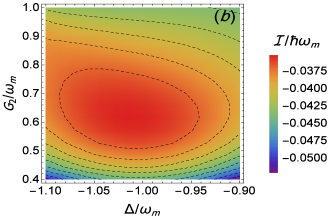
Figure 3: Plot of $\mathcal{I}$ (the difference between the energies of the mechanical modes $m_{1}$ and $m_{2}$), in units of $\hbar\omega_{m}$, against $\Delta/\omega_{m}$ and $G_{1}/\omega_{m}$ in (a), and against $\Delta/\omega_{m}$ and $G_{2}/\omega_{m}$ in (b). The parameters in (a) and (b) are, respectively, the same as in [Figs. 2(a) and 2(b)] and [Figs. 2(c) and 2(d)].

Quite remarkably, Fig. 2 shows that the state $\hat{\varrho}_{m_{1}m_{2}}$ of the two modes $m_{1}$ and $m_{2}$ can display two-way steering and even one-way steering. For example, [Figs. 2(a) and 2(b)] show that $\mathcal{G}^{m_{1}\rightarrow m_{2}}$ and $\mathcal{G}^{m_{2}\rightarrow m_{1}}$ are non-zero for $\Delta/\omega_{m}\approx-1$ and $G_{1}/\omega_{m}\geqslant 0.8$. This means that two-way steering can be detected over a wide range of operating parameters, which is proven in [22] to be a necessary resource needed for teleporting a coherent state with fidelity beyond the no-cloning threshold. Moreover, for $\Delta/\omega_{m}\approx-1$ and $0.45\leqslant G_{1}/\omega_{m}\leqslant 0.8$, we have $\mathcal{G}^{m_{1}\rightarrow m_{2}}=0$ and $\mathcal{G}^{m_{2}\rightarrow m_{1}}>0$, meaning that the state $\hat{\varrho}_{m_{1}m_{2}}$ is one-way steerable from $m_{2}\rightarrow m_{1}$. The different degree of steering observed between the directions $m_{1}\rightarrow m_{2}$ and $m_{2}\rightarrow m_{1}$ is also proven to provide the asymmetric guaranteed key rate achievable within a practical 1SDI-QKD [19].

Importantly, [Figs. 2(a) and 2(b)] show that the state $\hat{\varrho}_{m_{1}m_{2}}$ is one-way steerable from $m_{2}\rightarrow m_{1}$ for $G_{1}/G_{2}>1$, while it is one-way steerable in the reverse direction $m_{1}\rightarrow m_{2}$ for $G_{1}/G_{2}<1$ as depicted in [Figs. 2(c) and 2(d)]. Then, we conclude that the direction of one-way steering between the modes $m_{1}$ and $m_{2}$ could be merely manipulated through the ratio $G_{1}/G_{2}$ of the optomechanical coupling strengths, and then through the ratio $\wp_{1}/\wp_{2}$ of the input lasers powers following Eq. (13). This therefore provides an experimental flexible and feasible way to control the direction of one-way steering, in comparison with the loss-manipulating-method [54] that cannot be conveniently adjusted within the experimental operations.

To better explain the behavior of the direction of one-way steering observed in [Figs. 2(a) and 2(b)] and [Figs. 2(c) and 2(d)], we investigate the sign of the difference $\mathcal{I}=\mathcal{U}_{1}-\mathcal{U}_{2}$, where $\mathcal{U}_{j}=\frac{\hbar\omega_{m}}{2}(\langle\delta\hat{q}_{j}^{2}\rangle+\langle\delta\hat{p}_{j}^{2}\rangle)$ is the mean energy of the $j$th mechanical mode. From now on, we study $\mathcal{I}$ in units of $\hbar\omega_{m}$. Fig. 3(a) shows the difference $\mathcal{I}$ under the same circumstances of [Figs. 2(a) and 2(b)]. While, Fig. 3(b) shows $\mathcal{I}$ under the same circumstances of [Figs. 2(c) and 2(d)]. Manifestly, the direction of one-way steering is strongly influenced by the sign of $\mathcal{I}$, i.e., in Fig. 3(a) where $\mathcal{I}$ remains positive, one-way steering is occurred from $m_{2}\rightarrow m_{1}$ in [Figs. 2(a) and 2(b)]. Whereas, in Fig. 3(b) where $\mathcal{I}$ remains negative, one-way steering is occurred in the reverse direction $m_{1}\rightarrow m_{2}$ as illustrated in [Figs. 2(c) and 2(d)].

From a practical point of view, one-way steering from $m_{1}\rightarrow m_{2}$ can be interpreted as follows: Alice (owning mode $m_{1}$) and Bob (owning mode $m_{2}$) can implement the same Gaussian measurements on their shared state $\hat{\varrho}_{m_{1}m_{2}}$, however, obtain contradictory outcomes [55]. Essentially, Alice can convince Bob (who does not trust her) that their shared state $\hat{\varrho}_{m_{1}m_{2}}$ is entangled, while the converse is impossible. The most interesting application of asymmetric steering is that it provides security in 1SDI-QKD, where the measurement apparatus of one party only is untrusted.

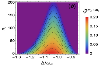
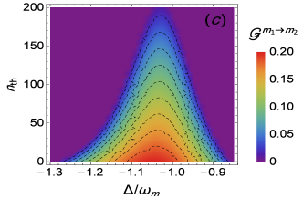
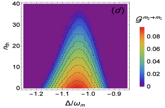
Figure 4: (a) and (b) show, respectively, $\mathcal{G}^{m_{1}\rightarrow m_{2}}$ and $\mathcal{G}^{m_{2}\rightarrow m_{1}}$ versus the normalized detuning $\Delta/\omega_{m}$ and the common mean thermal phonon number $n_{\text{th},1}=n_{\text{th},2}=n_{\text{th}}$ for $G_{1}/\omega_{m}=0.5$ and $G_{2}/\omega_{m}=0.4$. (c) and (d) show, respectively, $\mathcal{G}^{m_{1}\rightarrow m_{2}}$ and $\mathcal{G}^{m_{2}\rightarrow m_{1}}$ versus $\Delta/\omega_{m}$ and $n_{\text{th}}$ for $G_{1}/\omega_{m}=0.4$ and $G_{2}/\omega_{m}=0.5$. The other parameters are $\omega_{m}/2\pi=947~{}\mathrm{kHz}$, $\kappa/2\pi=215~{}\mathrm{kHz}$, $\gamma/2\pi=140~{}\mathrm{Hz}$, and $\zeta/\omega_{m}=0.1$.

Next, we continue by analysing the steerabilities $\mathcal{G}^{m_{1}\rightarrow m_{2}}$ and $\mathcal{G}^{m_{2}\rightarrow m_{1}}$ under influence of the common mean thermal phonon number $n_{\mathrm{th,1}}=n_{\mathrm{th,2}}=n_{\mathrm{th}}$ and the normalized detuning $\Delta/\omega_{m}$ for $\zeta/\omega_{m}=0.1$. In [Figs. 4(a) and 4(b)], we used $G_{1}/\omega_{m}=0.5$ and $G_{2}/\omega_{m}=0.4$. While in [Figs. 4(c) and 4(d)], we used $G_{1}/\omega_{m}=0.4$ and $G_{2}/\omega_{m}=0.5$. As can be seen, $\mathcal{G}^{m_{1}\rightarrow m_{2}}$ and $\mathcal{G}^{m_{2}\rightarrow m_{1}}$ are maximum close to $n_{\mathrm{th}}=0$ and $\Delta/\omega_{m}\approx-1$. However, they decrease by increasing $n_{\mathrm{th}}$, exhibiting rather different trends against thermal noise.

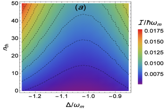
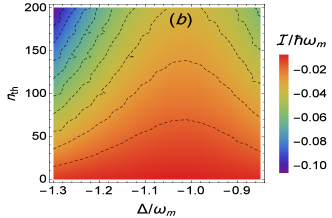
Figure 5: Plot of $\mathcal{I}$, in units of $\hbar\omega_{m}$, versus $\Delta/\omega_{m}$ and $n_{\text{th}}$. The parameters in (a) and (b) are, respectively, the same as in [Figs. 4(a) and 4(b)] and [Figs. 4(c) and 4(d)].

Strikingly, Fig. 4 shows that thermal noise, not only reduces the steerabilities $\mathcal{G}^{m_{1}\rightarrow m_{2}}$ and $\mathcal{G}^{m_{2}\rightarrow m_{1}}$, but may play a positive role in inducing and controlling one-way steering by the mediation of the ratio $G_{1}/G_{2}$. Indeed, in [Figs. 4(a) and 4(b)], where $G_{1}/G_{2}>1$, the steering $\mathcal{G}^{m_{1}\rightarrow m_{2}}$ disappears completely for $n_{\mathrm{th}}>35$. In contrast, $\mathcal{G}^{m_{2}\rightarrow m_{1}}$ can be detected even for $n_{\mathrm{th}}\approx 200$, meaning that the state $\hat{\varrho}_{m_{1}m_{2}}$ is one-way steerable from $m_{2}\rightarrow m_{1}$ for $35<n_{\text{th}}<200$. While, in [Figs. 4(c) and 4(d)], where $G_{1}/G_{2}<1$, $\mathcal{G}^{m_{2}\rightarrow m_{1}}$ vanishes completely for $n_{\mathrm{th}}>35$. In contrast $\mathcal{G}^{m_{1}\rightarrow m_{2}}$ still persist and can be detected for $n_{\mathrm{th}}\approx 200$, which means that the state $\hat{\varrho}_{m_{1}m_{2}}$ is one-way steerable from $m_{1}\rightarrow m_{2}$ for $35<n_{\text{th}}<200$. In fact, [Figs. 4(a) and 4(b)] show that Bob could stop Alice to steer his state by adding thermal noise to his mode $m_{2}$ provided that $G_{1}/G_{2}<1$ while he still can steer Alice’s mode $m_{1}$. The same operation can also be accomplished by Alice in the reverse direction as illustrated in [Figs. 4(c) and 4(d)].

Finally, Fig. 5(a) shows the difference $\mathcal{I}$ under the same circumstances of [Figs. 4(a) and 4(b)], while Fig. 5(b) shows $\mathcal{I}$ under the same circumstances of [Figs. 4(c) and 4(d)]. Also, we remark that the direction of one-way steering depends on the sign of $\mathcal{I}$, i.e., in Fig. 5(a) where $\mathcal{I}>0$, one-way steering emerges from $m_{2}\rightarrow m_{1}$ in [Figs. 4(a) and 4(b)]. Whereas, in Fig. 5(b) where $\mathcal{I}<0$, one-way steering emerges through the reverse direction $m_{1}\rightarrow m_{2}$ in [Figs. 2(c) and 2(d)]. These observations consist with the results illustrated in Figs. 2 and 3.

In [Figs. 2(c) and 2(d)] or [Figs. 4(c) and 4(d)], Alice’s manipulation can be viewed as part of a legal step in 1SDI-QKD protocol [20], where she can get one-way steering by performing local measurements on her mode $m_{1}$(e.g., adding thermal noise). While, in [Figs. 2(a) and 2(b)] or [Figs. 4(a) and 4(b)], Bob can obtain one-way steering in the reverse direction by performing local measurements on mode $m_{2}$, where his manipulation can be regarded either as a legitimate step or an adversarial attack in 1SDI-QKD protocol [20]. From this perspective, the presented one-way steering manipulation scheme can be connected with the 1SDI-QKD protocol, knowing that the security of such protocol depends fundamentally on the direction of steering [20].

4 Experimental detection of the generated optomechanical steering

A challenging aspect of any proposal involving quantum correlations creation between mechanical degrees of freedom is the actual experimental detection of the generated quantum correlations. Here, we discuss how the generated mechanical steerabilities $\mathcal{G}^{m_{1}\rightarrow m_{2}}$ and $\mathcal{G}^{m_{2}\rightarrow m_{1}}$ can be measured experimentally. For two optical modes, measuring their nonlocal correlations can be straightforwardly accomplished by the well-developed method of homodyne measurement [56]. In our case of two mechanical modes, the situation is less straightforward. However, the measurement can be indirectly performed by transferring adiabatically the quantum correlations from the two mechanical modes back to two auxiliary optical modes [42, 43]. Indeed, we assume that the $j$th mechanical mirror is perfectly reflecting in both sides, then a fixed and partially transmitted mirror can be placed instead it to form another Fabry-Pérot cavity. We denote by $c_{j}$ the $j$th intracavity auxiliary mode whose annihilation operator, dissipation rate, and effective detuning are $\hat{c}_{j}$, $\kappa_{c_{j}}$, and $\Delta_{c_{j}}$, respectively. Introducing the $j\text{th}$ mechanical annihilation operator $\delta\hat{m}_{j}=(\text{i}\delta\hat{p}_{j}+\delta\hat{q}_{j})/\sqrt{2}$, one can show that the fluctuation operator $\delta\hat{c}_{j}$ obeys an equation analogous to Eq. (6), i.e.,

$$\frac{d}{dt}\delta\hat{c}_{j}=-\left(\kappa_{c_{j}}+\mathrm{i}\Delta_{c_{j}}\right)\delta\hat{c}_{j}+\mathrm{i}\frac{G_{c_{j}}}{2}(\delta\hat{m}_{j}^{{\dagger}}+\delta\hat{m}_{j})+\sqrt{2\kappa_{c_{j}}}\hat{c}_{j}^{in}\text{,}$$ (19)

where $G_{c_{j}}$ is the effective coupling between the modes $c_{j}$ and $m_{j}$, with $\hat{c}_{j}^{in}$ being the vacuum radiation input noise acting on mode $c_{j}$.

Furthermore, assuming that the auxiliary mode is driven by a weak laser field, i.e., $\left|\langle\hat{o}_{j}\rangle\right|\gg\left|\langle\hat{c}_{j}\rangle\right|$, then the back-action of the auxiliary mode $c_{j}$ on the $j$th mirror can be safely neglected. Hence, the presence of the auxiliary mode cannot alter the system dynamics governed by Eqs. (2) and (3). Now, if we choose parameters so that $\Delta_{c_{j}}=\omega_{m}\gg$ $\kappa_{c_{j}}$, which is relevant for quantum-state transfer [43], Eq. (19) can be simplified by means of the rotating wave approximation [31], so to get

$$\frac{d}{dt}\delta\tilde{\hat{c}}_{j}=-\kappa_{c_{j}}\delta\tilde{\hat{c}}_{j}+\mathrm{i}\frac{G_{c_{j}}}{2}\delta\tilde{\hat{m}}_{j}+\sqrt{2\kappa_{c_{j}}}\tilde{\hat{c}}_{j}^{in},$$ (20)

where $\tilde{\Xi}=\Xi e^{i\omega_{m}t}$ for $\Xi\equiv\{\delta\hat{c}_{j},\delta\hat{m}_{j}$, $\hat{c}_{j}^{in}\}$. An optimal quantum-state transfer, from the mechanical mode $m_{j}$ to the auxiliary mode $c_{j}$, can be achieved when the later follows adiabatically the former, which requires $\kappa_{c_{j}}\gg G_{c_{j}}$ [45]. Hence, by setting $\frac{d}{dt}=0$ in Eq. (20) and using $\tilde{\hat{c}}_{j}^{out}=\sqrt{2\kappa_{c_{j}}}\delta\tilde{\hat{c}}_{j}-\tilde{\hat{c}}_{j}^{in}$ [50], we finally get

$$\tilde{\hat{c}}_{j}^{out}=\frac{\mathrm{i}G_{c_{j}}}{\sqrt{2\kappa_{c_{j}}}}\delta\tilde{\hat{m}}_{j}\ +\tilde{\hat{c}}_{j}^{in}.$$ (21)

The above equation shows that the mechanical covariance matrix (17) can be fully reconstructed via homodyning the output auxiliary fields using a single homodyne detector [56]. This therefore allows us the numerical estimation of the mechanical steerabilities $\mathcal{G}^{m_{1}\rightarrow m_{2}}$ and $\mathcal{G}^{m_{2}\rightarrow m_{1}}$.

5 Conclusions

In a double-cavity optomechanical system, stationary Gaussian quantum steering between two spatially separated mechanical modes is studied. The two cavities are coupled via an optical fiber, and driven by blue detuned lasers within the unresolved sideband regime. Using realistic experimental parameters, we showed that strong asymmetric steering can be achieved between the two considered modes. Furthermore, we showed that the direction of one-way steering can practically be controlled through the powers of the drive lasers and the temperatures of the cavities. This therefore provides a more flexible and feasible way to manipulate the direction of one-way steering in experimental operations. Besides, we revealed that the direction of one-way steering depends on the sign of the difference between the mean energies of the mechanical modes. Also, we discussed how the generated steering can be measured experimentally. The presented one-way steering manipulation scheme can be connected with the 1SDI-QKD protocol, knowing that the security of such protocol depends crucially on the direction of steering.

The feasibility of our proposal is verified using realistic experimental parameters within the unresolved sideband regime which makes the obtained results closer to the experimental reality. In addition, our scheme does not require additional squeezed light to drive the two cavities, which partly reduces the experimental realization requirement, and partly makes the presented scheme a very promising candidate for building up a tabletop network of optomechanical nodes connected by optical fibers. In practice, the losses—caused by absorption, scattering, etc—within the fiber couplers over long distance, can be overcome by using very-long ultra-low-loss fiber tapers [57] or optical amplifier technique based on devices that boost the signal power of the optical fiber without converting it to electrical signal [58].

This work may be meaningful for the distribution of long-distance trust which is of fundamental importance in secure quantum communication.

Data Availability Statement

No Data associated in the manuscript

References

• [1] A. Einstein, B. Podolsky, N. Rosen, Phys. Rev. 47, 777 (1935)
• [2] E. SchrΓΆdinger, Math. Proc. Cambridge Philos. Soc. 31, 555 (1935)
• [3] E. SchrΓΆdinger, Math. Proc. Cambridge Philos. Soc. 32, 446 (1936)
• [4] J. S. Bell, Physics 1, 195 (1964)
• [5] R. Uola, A. C. S. Costa, H. C. Nguyen, O. GΓΌhne, Rev. Mod. Phys. 92, 015001 (2020)
• [6] R. Horodecki, P. Horodecki, M. Horodecki, K. Horodecki, Rev. Mod. Phys. 81, 865 (2009)
• [7] H. M.Wiseman, S. J. Jones, A. C. Doherty, Phys. Rev. Lett. 98, 140402 (2007)
• [8] D. Yang, M. Horodecki, R. Horodecki, B. Synak-Radtke, Phys. Rev. Lett. 95, 190501 (2005)
• [9] A.C.S. Costa, R. Uola, O. GΓΌhne, Phys. Rev. A 98, 050104(R) (2018)
• [10] M.D. Reid, Phys. Rev. A 40, 913 (1989)
• [11] Z.Y. Ou, S. F. Pereira, H. J. Kimble, K. C. Peng, Phys. Rev. Lett. 68, 3663 (1992)
• [12] D. J. Saunders, S. J. Jones, H. M. Wiseman, G. J. Pryde, Nat. Phys. 6, 845 (2010)
• [13] D. H. Smith, G. Gillett, M. P. de Almeida, C. Branciard, A. Fedrizzi, T. J. Weinhold, A. Lita, B. Calkins, T. Gerrits, H. M. Wiseman, S. W. Nam, A. G. White, Nat. Commun. 3, 625 (2012)
• [14] E. G. Cavalcanti, S. J. Jones, H. M. Wiseman, M. D. Reid, Phys. Rev. A 80, 032112 (2009); I. Kogias, P. Skrzypczyk, D. Cavalcanti, A. AcΓ­n, G. Adesso, Phys. Rev. Lett. 115, 210401 (2015); H. Zhu, M. Hayashi, L. Chen, Phys. Rev. Lett. 116, 070403 (2016); S.P. Walborn, A. Salles, R.M. Gomes, F. Toscano, P.H. Souto Ribeiro, Phys. Rev. Lett. 106, 130402 (2011)
• [15] Y. Xiang, S. Cheng, Q. Gong, Z. Ficek, Q. He, PRX Quantum 3, 030102 (2022)
• [16] P. Skrzypczyk, M. NavascuΓ©s, D. Cavalcanti, Phys. Rev. Lett. 112, 180404 (2014)
• [17] M. Piani, J. Watrous, Phys. Rev. Lett. 114, 060404 (2015)
• [18] C. Weedbrook, S. Pirandola, R. Garcia-PatrΓ³n, N. J. Cerf, T. C. Ralph, J. H. Shapiro, S. Lloyd, Rev. Mod. Phys. 84, 621 (2012)
• [19] I. Kogias, A. R. Lee, S. Ragy, G. Adesso, Phys. Rev. Lett. 114, 060403 (2015)
• [20] C. Branciard, E. G. Cavalcanti, S. P. Walborn, V. Scarani, H. M. Wiseman, Phys. Rev. A 85, 010301(R) (2012)
• [21] M. D. Reid, Phys. Rev. A 88, 062338 (2013)
• [22] Q. He, L. Rosales-ZΓ‘rate, G. Adesso, M. D. Reid, Phys. Rev. Lett. 115, 180502 (2015)
• [23] L. Ali, M. Ikram, T. Abbas, I. Ahmad, J. Phys. B: Atom. Mol. and Opt. Phys. 54, 235501 (2021)
• [24] Y. Xiang, I. Kogias, G. Adesso, Q. He, Phys. Rev. A 95, 010101(R) (2017)
• [25] Y. Guo, S. Cheng, X. Hu, B.-H. Liu, E.-M. Huang, Y.-F. Huang, C.-F. Li, G.-C. Guo, E. G. Cavalcanti, Phys. Rev. Lett. 123, 170402 (2019)
• [26] H.-Y. Ku, S.-L. Chen, H.-B. Chen, N. Lambert, Y.-N. Chen, F. Nori, Phys. Rev. A 94, 062126 (2016)
• [27] Y. Xiang, B. Xu, L. MiΕ‘ta Jr., T. Tufarelli, Q. He, G. Adesso, Phys. Rev. A 96, 042326 (2017)
• [28] D.-Y. Kong, J. Xu, Y. Tian, F. Wang, X.-M. Hu, Phys. Rev. Res. 4, 013084 (2022)
• [29] X. Deng, Y. Xiang, C. Tian, G. Adesso, Q. He, Q. Gong, X. Su, C. Xie, K. Peng, Phys. Rev. Lett. 118, 230501 (2017)
• [30] S. Armstrong, M. Wang, R. Y. Teh, Q. Gong, Q. He, J. Janousek, H.-A. Bachor, M. D. Reid, P. K. Lam, Nat. Phys. 11, 167 (2015)
• [31] J. El Qars, Ann. Phys. (Berlin) 534(6), 2100386 (2022)
• [32] M. Aspelmeyer, T.J. Kippenberg, F. Marquardt, Rev. Mod. Phys. 86, 1391 (2014)
• [33] R. Peng, C. Zhao, Z. Yang, J. Yang, L. Zhou, Phys. Rev. A 107, 013507 (2023)
• [34] Q. Guo, M.-R. Wei, C.-H. Bai, Y. Zhang, G. Li, T. Zhang, Phys. Rev. Res. 5, 013073 (2023)
• [35] F.-X. Sun, D. Mao, Y.-T. Dai, Z. Ficek, Q.-Y. He, Q.-H. Gong, New J. Phys. 19, 123039 (2017)
• [36] S. Zheng, F. Sun, Y. Lai, Q. Gong, Q. He, Phys. Rev. A 99(2), 022335 (2019)
• [37] J. Li, S.-Y. Zhu, Phys. Rev. A 96(6), 062115 (2017)
• [38] H. Tan, L. Sun, Phys. Rev. A 92, 063812 (2015)
• [39] H. Tan, W. Deng, Q. Wu, G. Li, Phys. Rev. A 95, 053842 (2017)
• [40] J. El Qars, M. Daoud, R. Ahl Laamara, Phys. Rev. A 98, 042115 (2018)
• [41] J. Cheng, Y.-M. Liu, H.-F. Wang, X. Yi, Ann. Phys. (Berlin) 534(12), 2200315 (2022)
• [42] T. A. Palomaki, J. D. Teufel, R. W. Simmonds, K. W. Lehnert, Science, 342, 710 (2013)
• [43] D. Vitali, S. Gigan, A. Ferreira, H.R. BΓΆhm, P. Tombesi, A. Guerreiro, V. Vedral, A. Zeilinger, M. Aspelmeyer, Phys. Rev. Lett. 98, 030405 (2007)
• [44] F. Marquardt, J. P. Chen, A. A. Clerk, S. M. Girvin, Phys. Rev. Lett. 99, 093902 (2007)
• [45] R. Ghobadi, S. Kumar, B. Pepper, D. Bouwmeester, A.I. Lvovsky, C. Simon, Phys. Rev. Lett. 112, 080503 (2014)
• [46] J. D. Teufel, F. Lecocq, R. W. Simmonds, Phys. Rev. Lett. 116, 013602 (2016)
• [47] A. H. Safavi-Naeini, S. GrΓΆblacher, J. T. Hill, J. Chan, M. Aspelmeyer, O. Painter, Nature (London) 500, 185 (2013)
• [48] J.-Q. Liao, Q.-Q. Wu, F. Nori, Phys. Rev. A 89, 014302 (2014)
• [49] M. KoppenhΓΆfer, C. Padgett, J.V. Cady, V. Dharod, H. Oh, A. C. Bleszynski Jayich, A.A. Clerk, Phys. Rev. Lett. 130, 093603 (2023)
• [50] D. F. Walls, G. J. Milburn, Quantum Optics (Springer, Berlin, 1994)
• [51] R. Benguria, M. Kac, Phys. Rev. Lett. 46, 1 (1981)
• [52] E. X. DeJesus, C. Kaufman, Phys. Rev. A 35, 5288 (1987)
• [53] S. GrΓΆblacher, K. Hammerer, M. R. Vanner, M. Aspelmeyer, Nature 460, 724 (2009)
• [54] Z.-B. Yang, X.-D. Liu, X.-Y. Yin, Y. Ming, H.-Y. Liu, R.-C. Yang, Phys. Rev. Appl. 15, 024042 (2021); C.-G. Liao, H. Xie, R.-X. Chen, M.-Y. Ye, X.-M. Lin, Phys. Rev. A 101, 032120 (2020); H. Tan, W. Deng, L. Sun, Phys. Rev. A 99, 043834 (2019)
• [55] V. HΓ€ndchen, T. Eberle, S. Steinlechner, A. Samblowski, T. Franz, R.F. Werner, R. Schnabel, Nat. Photonics 6, 596 (2012)
• [56] V. D’Auria, S. Fornaro, A. Porzio, S. Solimeno, S. Olivares, M. G. A. Paris, Phys. Rev. Lett. 102, 020502 (2009)
• [57] G. Brambilla, V. Finazzi, D. J. Richardson, Opt. Express 12, 2258 (2004)
• [58] D. M. Baney, P. Gallion, R. S. Tucker, Opt. Fiber Technol. 6, 122 (2000)