Tied–boxed algebras

Abstract

We introduce two new algebras that we call tied–boxed Hecke algebra and tied–boxed Temperley–Lieb algebra. The first one is a subalgebra of the algebra of braids and ties introduced by Aicardi and Juyumaya, and the second one is a tied–version of the well known Temperley–Lieb algebra. We study their representation theory and give cellular bases for them. Furthermore, we explore a strong connection between the tied–boxed Temperley–Lieb algebra and the so–called partition Temperley–Lieb algebra given by Juyumaya. Also, we show that both structures inherit diagrammatic interpretations from a new class of monoids that we call boxed ramified monoids. Additionally, we give presentations for the singular part of the ramified symmetric monoid and for the boxed ramified monoid associated to the Brauer monoid.

1 Introduction

The algebra of braids and ties or simply the bt–algebra $\mathcal{E}_{n}(q)$ was introduced by Aicardi and Juyumaya in [34, 3] by means an abstracting procedure of the so–called Yokonuma–Hecke algebra [56, 37]. This algebra can be regarded as a generalization of the well known Iwahori–Hecke algebra $\mathcal{H}_{n}(q)$ [30], and has a rich interpretation as a diagram algebra involving both the classic braid generators and a new family of generators, called ties, which arise from the combinatorics of set partitions [3, 52]. The bt–algebra was introduced with the purpose of constructing new representations of the braid group, however, in recent years, this algebra and its derivatives have been studied from various perspectives.

The representation theory of the algebra of braids and ties was initiated by Ryom-Hansen in [52]. Specifically, he defined a tensor representation of $\mathcal{E}_{n}(q)$ which used to classify the simple modules of this algebra. As a consequence, he obtained a linear basis for the bt–algebra and proved that its dimension is $n!\mathfrak{b}_{n}$, where $\mathfrak{b}_{n}$ denotes the $n$th Bell number [29, A000110]. These results where used by Aicardi and Juyumaya in [4] to show that $\mathcal{E}_{n}(q)$ supports a Markov trace and so constructed polynomial invariants for classical and singular knots in the sense of Jones [31]. Aicardi and Juyumaya observed that their invariants can be recovered by a new class of knotted objects that called tied links, which in turn can be obtained by closing a new class of braided object that called tied braids [5]. Tied braids (of $n$ strands) form a monoid $T\mathcal{B}_{n}$ called the tied braid monoid, which play the role of algebraic counterpart for tied links just as the braid group is the algebraic counterpart of classical links by means the Alexander theorem [10]. Furthermore, this monoid of tied braids was shown to be a semidirect product $T\mathcal{B}_{n}=\mathcal{P}_{n}\rtimes\mathcal{B}_{n}$, where $\mathcal{P}_{n}$ denotes the monoid of set partitions of $[n]=\{1,\ldots,n\}$ together with the classic product given by refinement [8]. More results related to knot theory via the bt–algebra and its derivatives can be found in the literature, such as other invariants for tied and singular links [6, 8], generalizations of the bt–algebra [7, 21, 8, 11], tied links in other topological settings [22, 18], among others.

The complex generic representation theory of the algebra of braids and ties was studied by Banjo in [13]. For this purpose, she showed that the algebra $\mathcal{E}_{n}(1)$ is isomorphic to the so–called small ramified partition algebra [45], which is generated by some pairs of set partitions of $[n]$ called ramified partitions [46]. On the other hand, cellularity of the algebra of braids and ties was studied by the second author and Ryom-Hansen in [19]. Specifically, they constructed an explicit cellular basis for $\mathcal{E}_{n}(q)$, whose elements are indexed by a special type of pairs of multitableaux. This construction allowed them to define an explicit isomorphism between the bt–algebra and a direct sum of matrix algebras over certain wreath product algebras indexed by partitions of numbers, whose cellularity was studied by Geetha and Goodman in [24]. This last result was later generalized by Marin in [42] by defining bt–algebra versions for arbitrary Coxeter groups. See Subsection 3.1, Subsection 3.1.1 and Subsection 3.1.2.

A first generalization of the tied braid monoid was given by the first author and Juyumaya in [11] by replacing the respective factors of the semidirect product decomposition of $T\mathcal{B}_{n}$ with a monoid of set partitions [50] and a monoid acting in some Coxeter group. Another generalization was given by the same authors together with Aicardi in [2, 1]. Specifically, inspired by the work of Banjo [13], they introduced a new class of monoids, formed by ramified partitions, that called ramified monoids, which are defined for every submonoid of the partition monoid. See Subsection 2.3. Particularly, the algebra of braids and ties $\mathcal{E}_{n}(q)$ can be regarded as a $q$–deformation of the monoid algebra of the ramified monoid $\mathcal{R}(\mathcal{S}_{n})$ associated to the symmetric group $\mathcal{S}_{n}$. See Subsection 3.2. Also, due to their combinatorial background, ramified monoids have a rich interpretation in terms of diagrams, and thus any algebra obtained by deformation of their monoid algebras inherit this diagrammatic interpretation. The ramified monoid $\mathcal{R}(\mathcal{B}r_{n})$ associated with the Brauer monoid $\mathcal{B}r_{n}$ was studied in [2] and the ramified monoid associated with the symmetric inverse monoid was studied in [1]. At the time of writing this paper, the structure of the ramified monoid $\mathcal{R}(\mathcal{J}_{n})$ associated to the Jones monoid $\mathcal{J}_{n}$ is still unknown.

A tied version of the well known BMW algebra is the t–BMW algebra introduced by Aicardi and Juyumaya in [6], which can be regarded as deformation of the monoid algebra of $\mathcal{R}(\mathcal{B}r_{n})$. Just as there is no known structure for the monoid $\mathcal{R}(\mathcal{J}_{n})$, there also no a tied version of the Temperley–Lieb algebra that is obtained as a deformation of the monoid algebra of this monoid. However, there are two tied versions of this algebra that are not directly related to the monoid $\mathcal{R}(\mathcal{J}_{n})$. The first one is the partition Temperley–Lieb algebra $\operatorname{PTL}_{n}(q)$ introduced by Juyumaya in [36] in a purely algebraic manner. The second one is the tied Temperley–Lieb algebra introduced by Aicardi, Juyumaya and Papi in [9], which is related to a submonoid of $\mathcal{R}(\mathcal{J}_{n})$ called the planar ramified monoid of $\mathcal{J}_{n}$ [1]. A generalization of the partition Temperley–Lieb algebra was studied by Ryom-Hansen in [53]. Specifically, inspired by the construction of generalized Temperley–Lieb algebras given in [28], he introduced certain permutation modules, which can be regarded as $\mathcal{E}_{n}(q)$–submodules of a tensor space module introduced in [52]. To be precise, Ryom–Hansen proved that the annihilator ideal $\mathcal{I}$ of the action of $\mathcal{E}_{n}(q)$ on this tensor space module is a free $\Z[q,q^{-1}]$–module with a basis given by a dual cellular basis of the one in [19]. Thus, he obtained that the quotient $\mathcal{E}_{n}(q)/\mathcal{I}$ is a simultaneous generalization of the genelized Temperley–Lieb algebra and the partition Temperley–Lieb algebra. In particular, for $N=2$, it is obtained that $\mathcal{E}_{n}(q)/\mathcal{I}\simeq\operatorname{PTL}_{n}(q)$, and thus $\operatorname{PTL}_{n}(q)$ is cellular as well.

In the present paper, we introduce two tied–like algebras that inherit the diagrammatic interpretation from a new class of submonoids of the ramified ones, called boxed ramified monoids, which generalize a monoid in [2, Section 7]. We study the representation theory of these algebras and give cellular bases for them. The first one is a subalgebra of the algebra of braids and ties, which we call the tied–boxed Hecke algebra. The second one is a new tied version of the Temperley–Lieb algebra, which we call the tied–boxed Temperley–Lieb algebra. Additionally, we determine presentations for the singular part of the ramified monoid associated to the symmetric group and for the boxed ramified monoid associated to the Brauer monoid.

The paper is organized as follows.

In Section 2, we give the main combinatorial and algebraic ingredients that we will use along the paper. Specifically, we recall compositions and multicompositions (Subsection 2.1), set partitions and related monoids such as partition monoids and ramified monoids (Subsection 2.2 and Subsection 2.3), and also some cellular algebras such as the Iwahori–Hecke algebra and the Temperley–Lieb algebra (Subsection 2.4). Section 3 is devoted to recall the definition of algebra of braids and ties and some important results mainly coming from representation theory (Subsection 3.1). We also recall the ramified symmetric monoid, from which the bt–algebra inherits its diagram structure, and study its center (Subsection 3.2). In Section 4, we introduce a new family of monoids that we call boxed ramified monoids, which will give diagrammatic structures to the algebras that we will study in the following sections. These monoids are submonoids of the ramified ones, which are defined by imposing a linearity condition on the right components of ramified partitions.

In Section 5, we introduce the tied-boxed Hecke algebra $bH_{n}(q)$ by generators and relations and study its representation theory (Subsection 5.1). Specifically, we establish its connection with the algebra of braids and ties (Proposition 5.1), enabling us to compute its dimension (Theorem 5.4) and thereby obtain a faithful representation of $bH_{n}(q)$ in a tensor space module. Subsequently, we construct a complete set of orthogonal idempotents for $bH_{n}(q)$ (Proposition 5.8), leading to a decomposition of it into a direct sum of two–sided ideals. This allows us to provide an explicit cellular basis for $bH_{n}(q)$ indexed by linear set partitions and standard Young tableaux of the initial kind (Theorem 5.10). Furthermore, we present a diagrammatic representation of $bH_{n}(q)$ inherited from the boxed ramified monoid of the symmetric group $\mathcal{BR}(\mathcal{S}_{n})$ (Subsection 5.2). Specifically, we give a presentation for $\mathcal{BR}(\mathcal{S}_{n})$ (Theorem 5.13), concluding that the tied-boxed Hecke algebra is a $q$–deformation of the monoid algebra of $\mathcal{BR}(\mathcal{S}_{n})$. We also prove that the center of $\mathcal{BR}(\mathcal{S}_{n})$ coincides with the monoid of compositions of integers (Proposition 5.16). Additionally, we delve into the study of the singular part of $\mathcal{BR}(\mathcal{S}_{n})$ (Subsection 5.3), providing a presentation for it (Theorem 5.20).

Finally, in Section 6, we introduce the tied–boxed Temperley–Lieb algebra $bTL_{n}(q)$ as a quotient of the tied–boxed Hecke algebra by a two–sided ideal generated by Steinberg elements. We give a presentation for $bTL_{n}(q)$ (Proposition 6.1) and show that it can be decomposed as a direct sum of two–sided ideals, obtaining an explicit cellular basis for $bTL_{n}(q)$, which is indexed by multipartitions whose components have Young diagrams with at most two columns and standard multitableaux of the initial kind (Theorem 6.2). Then, we explore a strong connection between $bTL_{n}(q)$ and the partition Temperley–Lieb algebra $\operatorname{PTL}_{n}(q)$ (Subsection 6.1). Specifically, we prove that $\operatorname{PTL}_{n}(q)$ is isomorphic to a direct sum of matrix algebras over certain wreath product algebras, obtaining a formula for the dimension of $\operatorname{PTL}_{n}(q)$, which is confirmed in [53] by considering the case $N=2$ of the generalized partition Temperley–Lieb. We next observe that the natural embedding of $bH_{n}(q)$ in $\mathcal{E}_{n}(q)$ induces an embedding of $bTL_{n}(q)$ in $\operatorname{PTL}_{n}(q)$ (Corollary 6.6). Furthermore, we present a diagrammatic realization of $bTL_{n}(q)$ inherited from the boxed ramified monoid of the Jones monoid (Subsection 6.2). Specifically, we recall the presentation for $\mathcal{BR}(\mathcal{J}_{n})$ given in [2, Theorem 56] and conclude that the tied–boxed Temperley–Lieb algebra is a $q$–deformation of the monoid algebra of $\mathcal{BR}(\mathcal{J}_{n})$. (Theorem 6.7). Additionally, we study the boxed ramified monoid of the Brauer monoid (Subsection 6.3), providing a presentation for it (Theorem 6.12).

2 Preliminaries

For every pair of integers $m,n$ with $m\leq n$ we will denote by $[m,n]$ the discrete interval $\{m,\ldots,n\}$. Also, if $n$ is positive we set $[n]=[1,n]$ and $[n]_{0}=[0,n]$.

In what follows $n$ denotes a positive integer, and $\mathbb{S}$ denotes the ring $\mathbb{C}[q,q^{-1}]$, where $q$ is an indeterminate. Here, an $\mathbb{S}$–algebra means an associative $\mathbb{S}$–algebra with unit.

2.1 Compositions and multicompositions

A composition of size $n$ is a finite sequence $\mu$ formed by $\ell(\mu)$ elements in $[n]_{0}$, called parts, such that their sum is $n$. We denote by $\mathcal{C}_{n}$ the collection of compositions of $n$ with no null parts. It is known that $|\mathcal{C}_{n}|=2^{n-1}$ [29, A000079]. We say that a composition of $n$ is a partition if each pair of consecutive parts of it is nonincreasing. The collection of set partitions of $n$ will be denoted by $\operatorname{Par}_{n}$.

The Young diagram or simply the diagram of a composition $\mu=(\mu_{1},\ldots,\mu_{k})$ is the set $[\mu]$ defined as follows:

$$[\mu]=\{(i,j)\in\mathbb{N}^{2}\mid 1\leq j\leq\mu_{i}\}.$$

Elements of $[\mu]$ are called nodes and are represented by boxes located at positions $(i,j)$ of an array of size $\ell(\mu)\times n$. See Figure 1.

(4,2,3)

Figure 1: Young diagram of $(4,2,3)$.

A $\mu$–tableau is a bijection of $[\mu]$ with $[n]$, which is represented by inserting the image of each node, under this bijection, into its respective box. We denote by $\operatorname{Tab}(\mu)$ the set of all $\mu$–tableaux. A tableau is called row–standard if its entries increase from left to right. A row–standard tableau is called standard if it is defined by a partition and the entries of its columns increase from top to bottom. See Figure 2. We denote by $\operatorname{Std}(\mu)$ the collection of standard $\mu$–tableaux.

boxsize=1.3em,centertableaux1378,25,46

Figure 2: A standard $(4,2,2)$–tableau.

Observe that the symmetric group $\mathcal{S}_{n}$ acts on the right on the set $\operatorname{Tab}(\mu)$ by permuting the entries in each $\mu$–tableau. For $\mu\in\mathcal{C}_{n}$, we will denote by $\mathfrak{t}^{\mu}$ the standard $\mu$–tableau in which the numbers in $[n]$ are entered in increasing order from left to right along the rows of $[\mu]$. See Figure 3.

boxsize=1.3em,centertableaux1234,56,78

Figure 3: The standard $\mu$–tableau $\mathfrak{t}^{\mu}$ for $\mu=(4,2,2)$.

For each composition $\mu=(\mu_{1},\ldots,\mu_{k})\in\mathcal{C}_{n}$, we denote by $\mathcal{S}_{\mu}$ the stabilizer subgroup of the tableau $\mathfrak{t}^{\mu}$. This subgroup is called the Young subgroup of $\mu$, and is isomorphic to a direct product of symmetric groups, that is

$$\mathcal{S}_{\mu}\simeq\mathcal{S}_{\mu_{1}}\times\cdots\times\mathcal{S}_{\mu_{k}}.$$

For a row–standard $\mu$–tableau $\mathfrak{s}$, we denote by $d(\mathfrak{s})$ the unique permutation satisfying $\mathfrak{t}^{\mu}d(\mathfrak{s})=\mathfrak{s}$.

Given compositions $\mu,\mu^{\prime}$ of size $n$, we say that $\mu$ is finer than $\mu^{\prime}$, or that $\mu^{\prime}$ is coarser than $\mu$, denoted by $\mu\triangleleft\mu^{\prime}$, if $\mu^{\prime}$ can be obtained by adding consecutive parts of $\mu$. This relations gives to $\mathcal{C}_{n}$ a structure of lattice with supremum operation $\vee$. The pair $(\mathcal{C}_{n},\vee)$ will be called the monoid of compositions of $n$.

A multicomposition of size $n$ is a tuple ${\boldsymbol{\mu}}=(\mu^{(1)},\ldots,\mu^{(k)})$ such that $\mu^{(i)}\in\mathcal{C}_{n_{i}}$ and $n=n_{1}+\cdots+n_{k}$. We call ${\boldsymbol{\mu}}$ a multipartition if each $\mu_{i}$ is a partition. The collection of multicompositions (resp. multipartitions) of $n$ is denoted by $\mathcal{MC}_{n}$ (resp. $\mathcal{M}\mathrm{Par}_{n}$). For example, ${\boldsymbol{\mu}}=((1,2),(3,2,1),(1,1,1))$ is a multicomposition of $12$. The Young diagram or simply the diagram of a multicomposition ${\boldsymbol{\mu}}=(\mu^{(1)},\ldots,\mu^{(k)})$ is the set $[{\boldsymbol{\mu}}]$ defined as follows:

(2.1) $$[{\boldsymbol{\mu}}]=\{(i,j,c)\in\mathbb{N}^{3}\mid 1\leq j\leq\mu_{i}^{(c)},\,1\leq c\leq k\}.$$

In other words, the Young diagram of a multicomposition is the tuple formed by the diagrams of its components. See Figure 4.

$[{\boldsymbol{\mu}}]=\left(\,\yng(1,2)\,,\,\yng(3,2,1)\,,\,\yng(1,1,1)\,\right)$

Figure 4: The Young diagram of ${\boldsymbol{\mu}}=((1,2),(3,2,1),(1,1,1))$.

For ${\boldsymbol{\mu}}\in\mathcal{MC}_{n}$, a ${\boldsymbol{\mu}}$-multitableau is a tuple obtained from $[{\boldsymbol{\mu}}]$ by inserting the numbers of $[n]$ into its boxes. See Figure 5. We will write $\operatorname{shape}(\boldsymbol{\mathfrak{t}})={\boldsymbol{\mu}}$ to indicate that $\boldsymbol{\mathfrak{t}}$ is a ${\boldsymbol{\mu}}$-multitableau.

$\left(\,\scalebox{0.84}{\ytableausetup{boxsize=1.3em,centertableaux}\ytableaushort{7,5{10}}}\,,\,\scalebox{0.84}{\ytableausetup{boxsize=1.3em,centertableaux}\ytableaushort{49{12},16,3}}\,,\,\scalebox{0.84}{\ytableausetup{boxsize=1.3em,centertableaux}\ytableaushort{2,8,{11}}}\,\right)$

Figure 5: A ${\boldsymbol{\mu}}$-multitableau with ${\boldsymbol{\mu}}$ as in Figure 4.

A multitableau is called row–standard if each one of its components is row–standard. See Figure 5. A row–standard multitableau is called standard if it is defined by a multipartition and each one of its components is a standard tableau. See Figure 6. For each multicomposition ${\boldsymbol{\mu}}$ and each row–standard ${\boldsymbol{\mu}}$–multitableau ${\boldsymbol{\mathfrak{s}}}$, the elements $\boldsymbol{\mathfrak{t}}^{\boldsymbol{\mu}}$ and $d({\boldsymbol{\mathfrak{s}}})$ are defined in the obvious manner as generalizations of $\mathfrak{t}^{\mu}$ and $d(\mathfrak{s})$, respectively.

$\left(\,\scalebox{0.84}{\ytableausetup{boxsize=1.3em,centertableaux}\ytableaushort{5{10},7}}\,,\,\scalebox{0.84}{\ytableausetup{boxsize=1.3em,centertableaux}\ytableaushort{16{12},49,8}}\,,\,\scalebox{0.84}{\ytableausetup{boxsize=1.3em,centertableaux}\ytableaushort{2,8,{11}}}\,\right)$

Figure 6: A standard multitableu.

Let ${\boldsymbol{\mu}}=(\mu^{(1)},\ldots,\mu^{(k)})$ be a multicomposition of size $n$ such that $\mu^{(j)}\in\mathcal{C}_{n_{j}}$ for all $j\in[k]$. We denote by $\operatorname{\textbf{comp}}({\boldsymbol{\mu}})$ the composition given by the size of each component of ${\boldsymbol{\mu}}$. That is $\operatorname{\textbf{comp}}({\boldsymbol{\mu}})=(n_{1},\ldots,n_{k})$. For example, the composition associate to the multicomposition ${\boldsymbol{\mu}}=((1,2),(3,2,1),(1,1,1))$ is $\operatorname{\textbf{comp}}({\boldsymbol{\mu}})=(3,6,3)$.

2.2 Set partitions

In what follows $A$ denotes a nonempty set.

A set partition of $A$ is a collection of pairwise disjoint nonempty subsets of it, called blocks, such that their union is $A$. The collection of set partitions of $A$ is denoted by $\mathcal{P}(A)$, and $\mathcal{P}([n])$ is denoted by $\mathcal{P}_{n}$ instead. The cardinality of $\mathcal{P}_{n}$ is the $n$th Bell number $\mathfrak{b}_{n}$ [29, A000110].

Set partitions $\mathbf{I}=\{I_{1},\ldots,I_{k}\}$ of $[n]$ are denoted by $\mathbf{I}=(I_{a_{1}},\ldots,I_{a_{k}})$, where $\min(I_{a_{1}})<\cdots<\min(I_{a_{k}})$. These set partitions are usually represented by arc diagrams, which connect, in a transitive manner, the elements of $[n]$ that belong to the same block. See Figure 7. Also, we set $|\mathbf{I}|=k$ and $\|\mathbf{I}\|=(|I_{1}|,\ldots,|I_{k}|)$. For $\mathbf{I}\in\mathcal{P}_{n}$ and $i,j\in[n]$, we will denote by $i\sim_{\mathbf{I}}j$ the fact that $i,j$ belong to the same block of $\mathbf{I}$.

Figure 7: Set partition $(\{1,3,8\},\{2,5,7\},\{4,6\})$ of $[8]$.

Given $\mathbf{I},\mathbf{J}\in\mathcal{P}(A)$, we say that $\mathbf{I}$ is finer than $\mathbf{J}$, or that $\mathbf{J}$ is coarser than $\mathbf{I}$, denoted by $\mathbf{I}\preceq\mathbf{J}$, if each block of $\mathbf{J}$ is a union of blocks of $\mathbf{I}$. This relation gives to $\mathcal{P}(A)$ a structure of lattice with supremum operation $\vee$. The pair $(\mathcal{P}_{n},\vee)$ is called the monoid of set partitions of $[n]$. It was shown in [20, Theorem 2] that $\mathcal{P}_{n}$ can be presented by $\frac{n(n-1)}{2}$ [29, A000217] generators $e_{i,j}$ with $i<j$, subject to the following relations:

(2.2) $$e_{i,j}^{2}=e_{i,j},\quad e_{i,j}e_{r,s}=e_{r,s}e_{i,j},\quad e_{i,j}e_{i,k}=e_{i,j}e_{j,k}=e_{i,k}e_{j,k},$$

where each $e_{i,j}$ is the set partition of $[n]$ whose unique block that is not a singleton is $\{i,j\}$. See Figure 8.

Figure 8: Generators $e_{i,j}$ of $\mathcal{P}_{4}$.

Given $\mathbf{I}\in\mathcal{P}(A)$ and a subset $X$ of $A$, we set $\mathbf{I}\cap X=\{B\cap X\mid B\in\mathbf{I}\}\backslash\{\emptyset\}$ in $\mathcal{P}(X)$.

Observe that if $X$ is a subset of $A$ and $\mathbf{I}\in\mathcal{P}(X)$, then $\mathbf{I}$ can be naturally regarded as a set partition of $A$ by inserting to it the singletons $\{a\}$ with $a\in A\backslash X$. Now, if $\mathbf{I}\in\mathcal{P}(A)$ and $\mathbf{J}\in\mathcal{P}(B)$ for some set $B$, we will simply denote by $\mathbf{I}\vee\mathbf{J}$ the product of $\mathbf{I}$ with $\mathbf{J}$ regarded as elements of $\mathcal{P}(A\cup B)$.

A ramified partition of $A$ is a pair $(\mathbf{I},\mathbf{J})$ of set partitions of $A$ such that $\mathbf{I}\preceq\mathbf{J}$. Observe that $(\mathbf{I},\mathbf{J})$ can be regarded as a set partition of $\mathbf{I}$, in which two blocks of $\mathbf{I}$ belong to the same block of $(\mathbf{I},\mathbf{J})$ whenever both are contained in the same block of $\mathbf{J}$. The collection of ramified partitions of $A$ is denoted by $\mathcal{RP}(A)$, and $\mathcal{RP}([n])$ is denoted by $\mathcal{RP}_{n}$. We call $\mathcal{RP}(A)$, together with the product $(\mathbf{I},\mathbf{J})\vee(\mathbf{H},\mathbf{K})=(\mathbf{I}\vee\mathbf{H},\mathbf{J}\vee\mathbf{K})$, the monoid of ramified partitions of $A$.

2.3 The partition and the ramified monoids

Here, we will denote by $\mathfrak{C}_{n}$ instead of $\mathcal{P}_{2n}$ the collection of set partitions of $[2n]$. Set partitions in $\mathfrak{C}_{n}$ will be represented by strand diagrams, which are obtained from arc diagrams, by locating on top the elements of $[n]$ and at bottom the elements of $[n+1,2n]$ renumbered from $1$ to $n$. See Figure 9.

$$\vbox{\hbox{\includegraphics{pics/090.pdf}}}\,\,=\,\vbox{\hbox{\includegraphics{pics/095.pdf}}}$$

Figure 9: Set partition $(\{1,3,8\},\{2,5,7\},\{4,6\})$ of $[8]$.

For $\mathbf{I},\mathbf{J}\in\mathfrak{C}_{n}$, the concatenation $\mathbf{I}*\mathbf{J}$ of $\mathbf{I}$ with $\mathbf{J}$, is the set partition obtained by identifying the bottom elements of $\mathbf{I}$ with the top ones of $\mathbf{J}$ and so removing them. More specifically, if $X=\{x_{1},\ldots,x_{n}\}$ is a set that contains no elements of $[2n]$, then $\mathbf{I}*\mathbf{J}=(\mathbf{I}_{X}\vee\mathbf{J}^{X})\cap[2n]$, where $\mathbf{I}_{X}$ is obtained from $\mathbf{I}$ by replacing each $n+i$ by $x_{i}$ and $\mathbf{J}^{X}$ is obtained from $\mathbf{J}$ by replacing each $i$ by $x_{i}$. See Figure 10.

$$\vbox{\hbox{\includegraphics{pics/091.pdf}}}\,\,*\,\vbox{\hbox{\includegraphics{pics/092.pdf}}}\,\,\,=\,\,\vbox{\hbox{\includegraphics{pics/093.pdf}}}\,\,\,=\,\,\vbox{\hbox{\includegraphics{pics/094.pdf}}}$$

Figure 10: Set partition $(\{1,3,8\},\{2,5,7\},\{4,6\})$ of $[8]$.

The collection $\mathfrak{C}_{n}$ together with the concatenation product is called the partition monoid [32, 43, 44]. The collection of set partitions of $[2n]$ whose blocks contain exactly two elements forms a submonoid $\mathcal{B}r_{n}$ of $\mathfrak{C}_{n}$, called the Brauer monoid [14], which is presented by generators $s_{1},\ldots,s_{n-1}$ and $t_{1},\ldots,t_{n-1}$, subject to the relations [41, Theorem 3.1]:

(2.3) $$s_{i}^{2}=1;\qquad s_{i}s_{j}s_{i}=s_{j}s_{i}s_{j},\quad|i-j|=1;\qquad s_{i}s_{j}=s_{j}s_{i},\quad|i-j|>1;$$

(2.4) $$t_{i}^{2}=t_{i};\qquad t_{i}t_{j}t_{i}=t_{i},\quad|i-j|=1;\qquad t_{i}t_{j}=t_{j}t_{i},\quad|i-j|>1;$$

(2.5) $$s_{i}t_{j}t_{i}=s_{j}t_{i},\quad t_{i}t_{j}s_{i}=t_{i}s_{j},\quad|i-j|=1;\qquad t_{i}s_{i}=s_{i}t_{i}=t_{i};\qquad t_{i}s_{j}=s_{j}t_{i},\quad|i-j|>1.$$

The submonoid of $\mathcal{B}r_{n}$ presented by generators $s_{1},\ldots,s_{n-1}$ and relations in (2.3) corresponds to the symmetric group $\mathcal{S}_{n}$ of permutations of $[n]$, and coincides with the group of units of $\mathfrak{C}_{n}$. The submonoid $\mathcal{J}_{n}$ of $\mathcal{B}r_{n}$ presented by generators $t_{1},\ldots,t_{n}$ and relations in (2.4) is called the Jones monoid. It is well known that $|\mathcal{S}_{n}|$ is the $n$th factorial number $n!$ [29, A000142], and that $|\mathcal{J}_{n}|$ is the $n$th Catalan number $\mathfrak{c}_{n}$ [29, A000108].

For every submonoid $M$ of $\mathfrak{C}_{n}$, we denote by $\mathcal{R}(M)$ the collection of ramified partitions $(\mathbf{I},\mathbf{J})$ of $[2n]$ such that $\mathbf{I}\in M$. Ramified partitions $(\mathbf{I},\mathbf{J})$ in $\mathcal{R}(\mathfrak{C}_{n})$ are represented by diagrams of ties, which are obtained by connecting by ties the blocks in the strand diagram of $\mathbf{I}$ that are contained in the same block of $\mathbf{J}$. See Figure 11. The collection $\mathcal{R}(M)$ together with the product $(\mathbf{I},\mathbf{J})*(\mathbf{H},\mathbf{K})=(\mathbf{I}*\mathbf{J},\mathbf{H}*\mathbf{K})$ is called the ramified monoid of $M$. Observe that $M$ embeds inside $\mathcal{R}(M)$ through the identification $\mathbf{I}\mapsto(\mathbf{I},\mathbf{I})$.

Figure 11: Ramified partition $\left((\{1,3\},\{2\},\{4,6,8\},\{5\},\{7\}),(\{1,3,4,6,8\},\{2,5\},\{7\})\right)$ in $\mathcal{R}(\mathfrak{C}_{4})$.

As mentioned in [1, Proposition 2], the monoid $\mathcal{R}(\{1\})$ is isomorphic to $\mathcal{P}_{n}$ via the identification of $e_{i,j}$ with the ramified partition obtained by connecting by a tie the $i$th strand with the $j$th strand of the identity of $\mathfrak{C}_{n}$. See Figure 12. This implies that every ramified monoid contains $\mathcal{P}_{n}$ as a submonoid. We will use the same notation to denote $e_{i,j}$ as an element of $\mathcal{R}(\{1\})$.

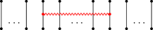
Figure 12: Generator $e_{i,j}$.

2.4 Cellular algebras

In this subsection we recall briefly the concept of a cellular algebra, introduced by Graham and Lerher in [26]. Later, we recall the Murphy’s standard basis of the Iwahori–Hecke algebra, which results to be a cellular basis. We will use this basis as an inspiration to construct cellular bases for the two algebras that we study in this paper: the tied–boxed Hecke algebra and the tied–boxed Temperley–Lieb algebra.

Let $R$ be an integral domain, and let $A$ to be an $R$–algebra which is free as an $R$–module. Consider $(\Lambda,\geq)$ to be a poset in which for each $\lambda\in\Lambda$ there is a finite indexing set $T(\lambda)$ and elements $c_{\mathfrak{s}\mathfrak{t}}^{\lambda}\in A$ such that $B:=\{c_{\mathfrak{s}\mathfrak{t}}^{\lambda}\mid\lambda\in\Lambda\text{ and }\mathfrak{s},\mathfrak{t}\in T(\lambda)\}$ is an $R$–basis of $A$. The pair $(B,\Lambda)$ is said to be a cellular basis of $A$ if:

1. The $R$–linear map $*:A\to A$ given by $(\mathop{c_{\mathfrak{s}\mathfrak{t}}^{\lambda}})^{*}=c_{\mathfrak{t}\mathfrak{s}}^{\lambda}$ is an algebra antiautomorphism of $A$.

2. For any $\lambda\in\Lambda,\;\mathfrak{t}\in T(\lambda)$ and $a\in A$ there is $r_{\mathfrak{v}}\in R$ such that for all $\mathfrak{s}\in T(\lambda)$

   $$c_{\mathfrak{s}\mathfrak{t}}^{\lambda}a\equiv\sum_{\mathfrak{v}\in T(\lambda)}r_{\mathfrak{v}}c_{\mathfrak{s}\mathfrak{v}}^{\lambda}\mod A^{\lambda},$$

   where the coefficient $r_{\mathfrak{v}}\in R$ do not depend on $\mathfrak{t}$, and $A^{\lambda}$ is the $R$–submodule of $A$ with basis:

   $$\{c_{\mathfrak{u}\mathfrak{v}}^{\mu}\mid\mu\in\Lambda\text{ such that }\mu>\lambda\text{ and }\mathfrak{u},\mathfrak{v}\in T(\mu)\}.$$

In this case, $A$ is said to be a cellular algebra, and the tuple $(\Lambda,T,B,\ast)$ is called the cell datum of it.

2.4.1 The Iwahori–Hecke algebra

Recall that the braid group $\mathcal{B}_{n}$ on $n$ strands [12] is the one presented by generators $\sigma_{1},\ldots,\sigma_{n-1}$ subject to the well known braid relations, that is:

(2.6) $$\sigma_{i}\sigma_{j}\sigma_{i}=\sigma_{j}\sigma_{i}\sigma_{j},\quad|i-j|=1;\qquad\sigma_{i}\sigma_{j}=\sigma_{j}\sigma_{i},\quad|i-j|>1.$$

The braid monoid $\mathcal{B}_{n}^{+}$ [23] is the submonoid of the braid group defined with the same presentation of $\mathcal{B}_{n}$.

The Iwahori–Hecke algebra $H_{n}(q)$ is the $\mathbb{S}$–algebra presented by generators $h_{1},\ldots,h_{n-1}$ subject to the braid relations together with a quadratic relation:

(2.7) $$h_{i}h_{j}h_{i}=h_{j}h_{i}h_{j},\quad|i-j|=1;\qquad h_{i}h_{j}=h_{j}h_{i},\quad|i-j|>1;\qquad h_{i}^{2}=1+(q-q^{-1})h_{i}.$$

Observe that $H_{n}(q)$ can be concerned as the quotient of the monoid algebra of $\mathcal{B}_{n}^{+}$ over $\mathbb{S}$, by the two–sided ideal defined by the quadratic relation in (2.7). Also, if $q=1$ it coincides with the group algebra of $\mathcal{S}_{n}$.

Due to the Matsumoto’s theorem [48], for each $w\in\mathcal{S}_{n}$ and each reduced expression $s_{i_{1}}\cdots s_{i_{k}}$ of it, the element $h_{w}:=h_{i_{1}}\cdots h_{i_{k}}$ is well defined in $H_{n}(q)$. Moreover, it is well known that $H_{n}(q)$ is a free $\mathbb{S}$–module with $\mathbb{S}$–basis $\{h_{w}\mid w\in\mathcal{S}_{n}\}$. Hence $\dim(H_{n}(q))=n!$. Another important $\mathbb{S}$–basis for $H_{n}(q)$ is the Murphy’s standard basis $B_{H_{n}}$ [49], which is indexed by pairs of standard tableaux:

(2.8) $$B_{H_{n}}=\{m_{\mathfrak{s}\mathfrak{t}}^{\lambda}:=h_{d(\mathfrak{s})}^{\ast}m_{\lambda}h_{d(\mathfrak{t})}\mid\lambda\in\operatorname{Par}_{n}\text{ and }\mathfrak{s},\mathfrak{t}\in\operatorname{Std}(\lambda)\}.$$

where $\ast:H_{n}(q)\to H_{n}(q)$ is the antiautomorphism given by $h_{w}^{*}=h_{w^{-1}}$ and $m_{\lambda}:=\sum_{w\in\mathcal{S}_{\lambda}}q^{\ell(w)}h_{w}$.

In [47], it was studied in detail the representation theory of $H_{n}(q)$ through its cellularity. Here, the Murphy’s standard basis $B_{H_{n}}$ is used as a cellular basis for the Iwahori–Hecke algebra.

2.4.2 The Temperley–Lieb algebra

For every integer $n\geq 3$, the Temperley–Lieb algebra $TL_{n}(q)$ is the $\mathbb{S}$–algebra presented by generators $h_{1},\ldots,h_{n-1}$ satisfying (2.7), subject to the following additional relations:

(2.9) $$h_{i,j}=0;\quad\text{where}\quad h_{i,j}=1+qh_{i}+qh_{j}+q^{2}h_{i}h_{j}+q^{2}h_{j}h_{i}+q^{3}h_{i}h_{j}h_{i},\qquad|i-j|=1.$$

The elements $h_{i,j}$ are called the Steinberg elements. Observe that $TL_{n}(q)$ is the quotient of $H_{n}(q)$ by the two–sided ideal generated by these elements. It is well know that $\dim(TL_{n}(q))=\mathfrak{c}_{n}$, the $m$th Catalan number [29, A000108].

It is worth to mention that there are several definitions of the Temperley–Lieb algebra [55, 38, 31]. In our definition, we consider the following changes with respect to the Härterich’s presentation [28].

$$\begin{array}[]{c|c}\text{H\"{a}rterich}&\text{Actual}\\ \hline\cr q&{q^{2}}^{{\color[rgb]{1,1,1}1}}\\ T_{s_{i}}&qh_{i}\end{array}$$

In [28], Härterich established a relation between the diagrammatical cellular basis of $TL_{n}(q)$ and the Murphy’s cellular basis of $H_{n}(q)$ given in (2.8). Indeed, from this basis he obtained a new cellular basis $B_{TL_{n}}$ for $TL_{n}(q)$ by considering only the standard tableaux with at most two columns. More precisely,

(2.10) $$B_{TL_{n}}=\{m_{\mathfrak{s}\mathfrak{t}}\mid\lambda\in\operatorname{Par}_{n}^{\leq 2}\text{ and }\mathfrak{s},\mathfrak{t}\in\operatorname{Std}(\lambda)\},$$

where $\operatorname{Par}_{n}^{\leq 2}$ is the subset formed by the partitions in $\operatorname{Par}_{n}$ whose Young diagrams have at most two columns.

2.4.3 The Young Hecke algebra and the Young Temperley–Lieb algebra

A ${\boldsymbol{\lambda}}$–multitableau $\boldsymbol{\mathfrak{t}}$ is called of the initial kind if the $i$th component of $\boldsymbol{\mathfrak{t}}$ contains exactly the numbers of the $i$th component of $\boldsymbol{\mathfrak{t}}^{\boldsymbol{\lambda}}$. For every ${\boldsymbol{\lambda}}\in\mathcal{M}\mathrm{Par}_{n}$, we set $T({\boldsymbol{\lambda}})=\{\boldsymbol{\mathfrak{t}}\in\operatorname{Std}({\boldsymbol{\lambda}})\mid\boldsymbol{\mathfrak{t}}\text{ is of the initial kind}\}$.

For every $\mu=(\mu_{1},\ldots,\mu_{k})\in\mathcal{C}_{n}$, the Young Hecke algebra $H_{\mu}$ (resp. Young Temperley–Lieb algebra $TL_{\mu}$) of $\mu$, is the subalgebra of $H_{n}(q)$ (resp. $TL_{n}(q)$) generated by the simple transpositions of $\mathcal{S}_{\mu}$, that is

$$H_{\mu}\simeq H_{\mu_{1}}\otimes\cdots\otimes H_{\mu_{k}},\qquad TL_{\mu}\simeq TL_{\mu_{1}}\otimes\cdots\otimes TL_{\mu_{k}}.$$

It is well known that the tensorial product of cellular algebras is cellular, see for example [24, Section 3.2]. Indeed, by using a similar argument as the one used in [24, Section 3.4], we obtain that the elements of the Murphy’s basis of $H_{\mu}$ are indexed by pairs of standard ${\boldsymbol{\lambda}}$–multitableaux of the initial kind, say ${\boldsymbol{\mathfrak{s}}}=(\mathfrak{s}_{1},\ldots,\mathfrak{s}_{k})$ and $\boldsymbol{\mathfrak{t}}=(\mathfrak{t}_{1},\ldots,\mathfrak{t}_{k})$, with the condition that $\operatorname{\textbf{comp}}({\boldsymbol{\lambda}})=\mu$. More precisely, if ${\boldsymbol{\lambda}}=(\lambda^{(1)},\ldots,\lambda^{(k)})$, then

$$B_{H_{\mu}}=\{m_{{\boldsymbol{\mathfrak{s}}}\boldsymbol{\mathfrak{t}}}^{\boldsymbol{\lambda}}\mid{\boldsymbol{\mathfrak{s}}},\boldsymbol{\mathfrak{t}}\in T({\boldsymbol{\lambda}}),\,{\boldsymbol{\lambda}}\in\mathcal{M}\mathrm{Par}_{n}\text{ and }\operatorname{\textbf{comp}}({\boldsymbol{\lambda}})=\mu\},\quad\text{where}\quad m_{{\boldsymbol{\mathfrak{s}}}\boldsymbol{\mathfrak{t}}}^{\boldsymbol{\lambda}}=m_{\mathfrak{s}_{1}\mathfrak{t}_{1}}^{\lambda^{(1)}}\cdots m_{\mathfrak{s}_{k}\mathfrak{t}_{k}}^{\lambda^{(k)}}.$$

Similarly, the Murphy’s basis of $TL_{\mu}$ is the set

$$B_{TL_{\mu}}=\{m_{{\boldsymbol{\mathfrak{s}}}\boldsymbol{\mathfrak{t}}}^{\boldsymbol{\lambda}}\mid{\boldsymbol{\mathfrak{s}}},\boldsymbol{\mathfrak{t}}\in T({\boldsymbol{\lambda}}),\,{\boldsymbol{\lambda}}\in\mathcal{M}\mathrm{Par}_{n}^{\leq 2}\text{ and }\operatorname{\textbf{comp}}({\boldsymbol{\lambda}})=\mu\},$$

where $\mathcal{M}\mathrm{Par}_{n}^{\leq 2}=\{(\lambda^{(1)},\ldots,\lambda^{(k)})\in\mathcal{M}\mathrm{Par}_{n}\mid\lambda^{(i)}\in\operatorname{Par}_{n}^{\leq 2}\text{ for all }i\in[k]\}$.

3 The algebra of braids and ties

The algebra of braids and ties [3], or simply the bt–algebra, is the $\mathbb{S}$–algebra $\mathcal{E}_{n}(q)$ presented by generators $e_{1},\ldots,e_{n-1}$ and $g_{1},\ldots,g_{n-1}$, subject to the following relations:

(3.1) $$e_{i}^{2}=e_{i};\qquad e_{i}e_{j}=e_{j}e_{i};$$

(3.2) $$g_{i}g_{j}g_{i}=g_{j}g_{i}g_{j},\quad|i-j|=1;\qquad g_{i}g_{j}=g_{j}g_{i},\quad|i-j|>1;$$

(3.3) $$g_{i}e_{i}=e_{i}g_{i};\qquad g_{i}e_{j}=e_{j}g_{i},\quad|i-j|>1;$$

(3.4) $$e_{i}g_{j}g_{i}=g_{j}g_{i}e_{j},\quad e_{i}e_{j}g_{j}=e_{i}g_{j}e_{i}=g_{j}e_{i}e_{j},\quad|i-j|=1;$$

(3.5) $$g_{i}^{2}=1+(q-q^{-1})e_{i}g_{i}.$$

Observe that, due to (3.5), each $g_{i}$ is invertible with inverse $g_{i}^{-1}=g_{i}-(q-q^{-1})e_{i}$.

3.1 Representation theory

For $n,r$ positive integers satisfying $n\leq r$ and $V$ to be the free $\mathbb{S}$–module with basis $\{v_{i}^{a}\mid i\in[n],a\in[r]\}$, we define the operators $\mathbf{E},\mathbf{G}\in\operatorname{End}_{S}(V^{\otimes 2})$ as follows:

(3.6) $$(v_{i}^{a}\otimes v_{j}^{b})\mathbf{E}=\begin{cases}0&\text{if }a\neq b,\\ v_{i}^{a}\otimes v_{j}^{b}&\text{if }a=b,\end{cases}$$

and

(3.7) $$(v_{i}^{a}\otimes v_{j}^{b})\mathbf{G}=\begin{cases}v_{i}^{a}\otimes v_{j}^{b}&\text{if }a\neq b,\\ qv_{i}^{a}\otimes v_{j}^{b}&\text{if }a=b,\;i=j,\\ v_{j}^{a}\otimes v_{i}^{b}&\text{if }a=b,\;i>j,\\ (q-q^{-1})v_{i}^{a}\otimes v_{j}^{b}+v_{j}^{b}\otimes v_{i}^{a}&\text{if }a=b,\;i<j.\end{cases}$$

These ones can be extended to operators $\mathbf{E}_{i}$ and $\mathbf{G}_{i}$ acting on the tensor space $V^{\otimes n}$ by letting $\mathbf{E}$ and $\mathbf{G}$ act on the $i$th and $(i+1)$th factors.

Theorem 3.1 ([52, Corollary 4]).

The map $\rho:\mathcal{E}_{n}\to\operatorname{End}_{S}(V^{\otimes n})$ given by $g_{i}\mapsto\mathbf{G}_{i}$ and $e_{i}\mapsto\mathbf{E}_{i}$ defines a faithful representation of $\mathcal{E}_{n}$.

Now, we recall some important elements of $\mathcal{E}_{n}(q)$.

Given $w\in\mathcal{S}_{n}$ and $s_{i_{1}}\cdots s_{i_{k}}$ a reduced expression of it, we set $g_{w}=g_{i_{1}}\cdots g_{i_{k}}$, and put $g_{\operatorname{id}}=1\in\mathbb{S}$. From Matsumoto’s theorem [48], the element $g_{w}$ is independent on the choice of the reduced expression.

For $i,j\in[n-1]$, define $e_{i,j}$, recursively, as follows:

(3.8) $$e_{i,i+1}=e_{i}\quad\text{and}\quad e_{i,j}=g_{i}\cdots g_{j-1}e_{j}g_{j-1}^{-1}\cdots g_{i}^{-1}\quad\text{whenever}\quad j>i+1.$$

For every subset $B=\{i_{1}<\cdots<i_{r}\}$ of $[n]$, define

(3.9) $$E_{B}=\prod_{j=1}^{r-1}e_{i_{j},\,i_{j+1}},\quad\text{where}\quad E_{B}=1\quad\text{if}\quad|B|=1.$$

Given a set partition $\mathbf{I}=\{I_{1},\ldots,I_{k}\}\in\mathcal{P}_{n}$, we set

(3.10) $$E_{\mathbf{I}}=\prod_{i=1}^{k}E_{I_{i}}.$$

The elements $E_{B}$ and $E_{\mathbf{I}}$ were originally introduced by Ryom–Hansen [52] in a slightly different manner, however, as it was mentioned in [8], both definitions are equivalent. We will use the definitions in (3.9) and (3.10) because they are more useful for our purposes.

With the above notations it was shown in [52, Theorem 3] that the bt–algebra is a free $\mathbb{S}$–module with basis $\{E_{\bf I}g_{w}\mid\mathbf{I}\in\mathcal{P}_{n},\,w\in\mathcal{S}_{n}\}$. Thus, the dimension of $\mathcal{E}_{n}(q)$ is $\mathfrak{b}_{n}n!$. Furthermore, the elements $E_{\mathbf{I}}$ and $g_{w}$ satisfy the relation $E_{\mathbf{I}}g_{w}=g_{w}E_{\mathbf{I}w}$, where $w$ acts on $\mathbf{I}$ by permuting the elements of its blocks.

3.1.1 Ideal decomposition of $\mathcal{E}_{n}(q)$

Here, we recall some results from [19, Subsection 6.1].

Let $\mu:\mathcal{P}_{n}\times\mathcal{P}_{n}\to\Z$ to be the Möebius function over the lattice $(\mathcal{P}_{n},\preceq)$, defined in [19, Section 3.2].

Now, for every $\mathbf{I}\in\mathcal{P}_{n}$, we define

(3.11) $$\mathbb{E}_{\mathbf{I}}=\sum_{\mathbf{J}\succeq\mathbf{I}}\mu(\mathbf{I},\mathbf{J})E_{\mathbf{J}}.$$

From this standard construction, due to Solomon [54], we obtain a set of orthogonal idempotents $\{\mathbb{E}_{\mathbf{I}}\mid\mathbf{I}\in\mathcal{P}_{n}\}$ over $\mathcal{E}_{n}(q)$. Moreover, the elements $\mathbb{E}_{\mathbf{I}}$ satisfy the following relations with the basis elements of $\mathcal{E}_{n}(q)$.

(3.12) $$\mathbb{E}_{\mathbf{I}}g_{w}=g_{w}\mathbb{E}_{\mathbf{I}w}\qquad\text{ and }\qquad\mathbb{E}_{\mathbf{I}}\mathbf{E}_{\mathbf{J}}=\begin{cases}\mathbb{E}_{\mathbf{I}}&\text{if }\mathbf{J}\preceq\mathbf{I},\\ 0&\text{otherwise.}\end{cases}$$

In particular, we observe that $\{\mathbb{E}_{\mathbf{I}}g_{w}\mid w\in\mathcal{S}_{n},\;\mathbf{I}\in\mathcal{P}_{n}\}$ is another $\mathbb{S}$–basis for $\mathcal{E}_{n}(q)$.

For every $\alpha\in\operatorname{Par}_{n}$, we say that $\mathbf{I}=(I_{a_{1}},\ldots,I_{a_{k}})\in\mathcal{P}_{n}$ is of type $\alpha$, denoted by $|\mathbf{I}|=\alpha$, if there is a permutation $w\in\mathcal{S}_{n}$ such that $(|I_{a_{1}w}|,\ldots,|I_{a_{k}w}|)=\alpha$. Thus, we define the following element of $\mathcal{E}_{n}(q)$:

(3.13) $$\mathbb{E}_{\alpha}\,=\sum_{\mathbf{I}\in\mathcal{P}_{n},\,|\mathbf{I}|=\alpha}\mathbb{E}_{\mathbf{I}}.$$

The set $\{\mathbb{E}_{\alpha}\mid\alpha\in\operatorname{Par}_{n}\}$ is a family of central orthogonal idempotents of $\mathcal{E}_{n}(q)$ which is also complete, that is:

$$\sum_{\alpha\in\operatorname{Par}_{n}}\mathbb{E}_{\alpha}=1.$$

As a consequence we obtain that $\mathcal{E}_{n}(q)$ can be decomposed as a direct sum of two–side ideals:

(3.14) $$\mathcal{E}_{n}(q)=\bigoplus_{\alpha\in\operatorname{Par}_{n}}\mathcal{E}_{n}^{\alpha}(q),\quad\text{where}\quad\mathcal{E}_{n}^{\alpha}(q)=\mathbb{E}_{\alpha}\mathcal{E}_{n}(q).$$

Moreover, observe that the ideals $\mathcal{E}_{n}^{\alpha}(q)$ are also $\mathbb{S}$–algebras with identities $\mathbb{E}_{\alpha}$ and $\mathbb{S}$–bases:

$$\{\mathbb{E}_{\mathbf{I}}g_{w}\mid w\in\mathcal{S}_{n},\,|\mathbf{I}|=\alpha\}$$

In particular, $\dim\mathcal{E}_{n}^{\alpha}(q)=\mathfrak{b}_{n}(\alpha)n!$, where $\mathfrak{b}_{n}(\alpha)$ is the number of set partition having type $\alpha$ [29, A036040].

3.1.2 Isomorphism theorem for $\mathcal{E}_{n}(q)$

It was shown in [19, Theorem 64] that $\mathcal{E}_{n}(q)$ is isomorphic to a direct sum of matrix algebras with coefficients over certain wreath algebras introduced in [24]. The key point to establish this isomorphism is the construction of a cellular basis $\{m_{\mathbbm{s}\mathbbm{t}}^{\Lambda}\}$, which is indexed by a special type of pairs of multitableaux.

We first recall the more relevant elements in the construction of cell datum of $\mathcal{E}_{n}(q)$ given in [19]. For more details of this construction the reader should consult [19, Section 6].

The poset, denoted by $\mathcal{L}_{n}$, is the set of pairs of multipartitions $({\boldsymbol{\lambda}}\mid{\boldsymbol{\mu}})$, where ${\boldsymbol{\lambda}}=(\lambda^{(1)},\ldots,\lambda^{(k)})$ is an increasing multipartition of $n=n_{1}+\cdots+n_{k}$ (see this definition at the beginning of [19, Section 3.3]) with $\lambda^{(j)}\in\mathcal{C}_{n_{j}}$ for all $j\in[k]$, and ${\boldsymbol{\mu}}=(\mu^{(1)},\ldots,\mu^{(j)})$ with $\mu^{(i)}\in\operatorname{Par}_{m_{i}}$ and each $m_{i}$ being the multiplicities of equal $\lambda^{(i)}$’s in ${\boldsymbol{\lambda}}$. See Figure 13.

$\left(\left(\ytableausetup{boxsize=1.05em,centertableaux}\ydiagram{1},\ytableausetup{boxsize=1.05em,centertableaux}\ydiagram{1},\ytableausetup{boxsize=1.05em,centertableaux}\ydiagram{1},\ytableausetup{boxsize=1.05em,centertableaux}\ydiagram{1,1},\ytableausetup{boxsize=1.05em,centertableaux}\ydiagram{2,1},\ytableausetup{boxsize=1.05em,centertableaux}\ydiagram{2,1},\ytableausetup{boxsize=1.05em,centertableaux}\ydiagram{3}\right)\;\bigg{|}\;\left(\ytableausetup{boxsize=1.05em,centertableaux}\ydiagram{2,1},\ytableausetup{boxsize=1.05em,centertableaux}\ydiagram{1},\ytableausetup{boxsize=1.05em,centertableaux}\ydiagram{2},\ytableausetup{boxsize=1.05em,centertableaux}\ydiagram{1}\right)\right).$

Figure 13: An element of $\mathcal{L}_{14}$.

In what follows $\Lambda=({\boldsymbol{\lambda}}\mid{\boldsymbol{\mu}})\in\mathcal{L}_{n}$ with ${\boldsymbol{\lambda}}=(\lambda^{(1)},\ldots,\lambda^{(k)})$ and ${\boldsymbol{\mu}}=(\mu^{(1)},\ldots,\mu^{(j)})$ as above.

We define the linear set partition of $[n]$ associated to ${\boldsymbol{\lambda}}$ as follows. First, to each component $\lambda^{(j)}$ of ${\boldsymbol{\lambda}}$, we fix a subset $I_{j}$ of $[n]$ defined as follows:

$$I_{j}=\begin{cases}[1,n_{1}]&\text{if }j=1,\\ [n_{1}+\cdots+n_{j-1}+1,n_{1}+\cdots+n_{j}]&\text{if }j>1.\end{cases}$$

Then, the linear set partition associated to ${\boldsymbol{\lambda}}$ is given by $\mathbf{I}_{\boldsymbol{\lambda}}=\{I_{1},\ldots,I_{k}\}$. For example, the linear set partition associated to the multicomposition ${\boldsymbol{\lambda}}=((2,1),(3,2,1),(1,1,1))$ is $\mathbf{I}_{{\boldsymbol{\lambda}}}=\{[1,3],[4,9],[10,12]\}$.

Let $\mathcal{S}_{\Lambda}$ the stabilizer subgroup of the set partition $\mathbf{I}_{{\boldsymbol{\lambda}}}$. We denote by $\mathcal{S}_{\Lambda}^{m}$ the subgroup of $\mathcal{S}_{\Lambda}$ consisting of the order preserving permutations of the blocks of $\mathbf{I}_{\boldsymbol{\lambda}}$ that correspond to equal $\lambda^{(i)}$’s, that is

$$\mathcal{S}_{\Lambda}^{m}\simeq\mathcal{S}_{m_{1}}\times\cdots\times\mathcal{S}_{m_{r}}.$$

Indeed, $\mathcal{S}_{\Lambda}^{m}$ is generated by the permutations $B_{j}\in\mathcal{S}_{n}$, of minimal length, that interchange the blocks $\mathbf{I}_{j}$ and $\mathbf{I}_{j+1}$ of $\mathbf{I}_{{\boldsymbol{\lambda}}}$ whenever $\lambda^{(j)}=\lambda^{(j+1)}$. Moreover, we observe that $\mathcal{S}_{\Lambda}^{m}$ does not depend on ${\boldsymbol{\mu}}$ but on ${\boldsymbol{\lambda}}$.

For example, if ${\boldsymbol{\lambda}}=((1),(1),(1),(1,1,1),(1,1,1),(2,1),(2,1),(4))$, the following elements generate the subgroup $\mathcal{S}_{\Lambda}^{m}\leq\mathcal{S}_{20}$ with $\Lambda=({\boldsymbol{\lambda}}\mid\underline{\quad}\,)$:

$$B_{1}=s_{1},\quad B_{2}=s_{2},\quad B_{3}=(s_{6}s_{5}s_{4})(s_{7}s_{6}s_{5})(s_{8}s_{7}s_{6})\quad\text{ and }\quad B_{4}=(s_{12}s_{11}s_{10})(s_{13}s_{12}s_{11})(s_{14}s_{13}s_{12}).$$

Now, suppose that $s_{i_{1}}\cdots s_{i_{r}}$ is a reduced expression for $B_{i}\in\mathcal{S}_{\Lambda}^{m}$. Due to [19, Lemma 46], we have an embedding $\iota:\mathbb{S}\mathcal{S}_{\Lambda}^{m}\hookrightarrow\mathcal{E}_{n}$ given by $\iota(B_{i})=\mathbb{B}_{i}$, where $\mathbb{B}_{i}=\mathbb{E}_{\mathbf{I}_{{\boldsymbol{\lambda}}}}g_{i_{1}}\cdots g_{i_{r}}$. Furthermore, if $w=s_{j_{1}}\cdots s_{j_{k}}$ is a reduced expression for $w$, we can define $\mathbb{B}_{w}=\mathbb{B}_{j_{1}}\cdots\mathbb{B}_{j_{k}}$, which does not depend on the choice of the reduced expression for $w$.

We say that $\mathbbm{s}$ $=({\boldsymbol{\mathfrak{s}}}\mid\boldsymbol{\mathfrak{u}})$ is a standard $\Lambda$–tableau if the following conditions hold:

1. ${\boldsymbol{\mathfrak{s}}}$ is a standard ${\boldsymbol{\lambda}}$–multitableau in the usual sense.

2. ${\boldsymbol{\mathfrak{s}}}=(\mathfrak{s}^{(1)},\ldots,\mathfrak{s}^{(k)})$ is an increasing multitableau. By increasing we here mean that $i<j$ if and only if $\min(\mathfrak{s}^{(i)})<\min(\mathfrak{s}^{(j)})$ whenever $\operatorname{shape}(\mathfrak{s}^{(i)})=\operatorname{shape}(\mathfrak{s}^{(j)})$, where $\min(\mathfrak{s})$ is the function that reads off the minimal entry of the tableau $\mathfrak{s}$.

3. $\boldsymbol{\mathfrak{u}}$ is a stardard ${\boldsymbol{\mu}}$–multitableau of the initial kind.

We will denote by $\operatorname{Std}(\Lambda)$ the set of standard $\Lambda$–tableaux.

The Murphy element corresponding to $\Lambda$ is $m_{\Lambda}=\mathbb{E}_{\mathbf{I}_{{\boldsymbol{\lambda}}}}x_{{\boldsymbol{\lambda}}}b_{{\boldsymbol{\mu}}}$, where $x_{{\boldsymbol{\lambda}}}=x_{\lambda^{(1)}}\cdots x_{\lambda^{(k)}}$ and $b_{{\boldsymbol{\mu}}}=b_{\mu^{(1)}}\cdots b_{\mu^{(j)}}$, whose factors we explain below.

The element $\mathbb{E}_{\mathbf{I}_{{\boldsymbol{\lambda}}}}$ is the idempotent associated to the linear set partition $\mathbf{I}_{{\boldsymbol{\lambda}}}$ in (3.11). If $H(\lambda^{(j)})$ denotes the Iwahori–Hecke algebra with linear basis $\{h_{i}\mid i\in\mathbf{I}_{\boldsymbol{\lambda}}\}$, then the factor $x_{\lambda^{(i)}}$ can be seen as the image of the Murphy element of the Iwahori–Hecke algebra $H(\lambda^{(j)})$ through of the embedding $H(\lambda^{(j)})\hookrightarrow\mathcal{E}_{n}$ given by $h_{i}\mapsto g_{i}$. Similarly, the factor $b_{\mu^{(i)}}$ can be seen as the image of the $q=1$ specialization of the Murphy element $m_{\mu^{(i)}}\in H(\mu^{(j)})$ through of the embedding $\iota:\mathbb{S}\mathcal{S}_{\Lambda}^{m}\hookrightarrow\mathcal{E}_{n}$ defined above.

For standard $\Lambda$–tableaux $\mathbbm{s}$ $=({\boldsymbol{\mathfrak{s}}}\mid\boldsymbol{\mathfrak{u}})$ and $\mathbbm{t}$ $=(\boldsymbol{\mathfrak{t}}\mid\boldsymbol{\mathfrak{v}})$, the elements of the cellular basis of $\mathcal{E}_{n}$ are given by:

(3.15) $$\text{$m_{\mathbbm{s}\mathbbm{t}}^{\Lambda}$}=\,g_{d({\boldsymbol{\mathfrak{s}}})}^{*}\mathbb{E}_{\mathbf{I}_{{\boldsymbol{\lambda}}}}x_{{\boldsymbol{\lambda}}}\mathbb{B}_{d(\boldsymbol{\mathfrak{u}})}^{*}b_{{\boldsymbol{\mu}}}\mathbb{B}_{d(\boldsymbol{\mathfrak{v}})}g_{d(\boldsymbol{\mathfrak{t}})},$$

where $\ast$ is the antiautomorphism given by $e_{i}^{*}=e_{i}$ and $g_{i}^{*}=g_{i}$.

Theorem 3.2 ([19, Theorem 57]).

For each $\alpha\in\mathcal{P}_{n}$, the subalgebras $\mathcal{E}_{n}^{\alpha}(q)$ are cellular with cellular bases:

$$\mathcal{B}_{\alpha}=\{m_{\mathbbm{s}\mathbbm{t}}^{\Lambda}\mid\Lambda\in\mathcal{L}_{n}(\alpha),\,\mathbbm{s},\mathbbm{t}\in{\rm Std}(\Lambda)\},$$

where $\mathcal{L}_{n}(\alpha)=\{({\boldsymbol{\lambda}}\mid{\boldsymbol{\mu}})\mid\operatorname{\textbf{comp}}({\boldsymbol{\lambda}})=\alpha\}$.

As an immediate consequence, we get that $\mathcal{E}_{n}(q)$ is cellular with cellular basis:

$$\mathcal{B}_{\mathcal{E}_{n}}=\{m_{\mathbbm{s}\mathbbm{t}}^{\Lambda}\mid\Lambda\in\mathcal{L}_{n},\,\mathbbm{s},\mathbbm{t}\in\operatorname{Std}(\Lambda)\}.$$

Before state the main theorem of this subsection we need to recall some important ingredients.

Similarly to the definition of the subgroup $\mathcal{S}_{\Lambda}^{m}$ of $\mathcal{S}_{\Lambda}$, we define $\mathcal{S}_{\Lambda}^{k}$ as the subgroup of $\mathcal{S}_{\Lambda}$ consisting of the order preserving permutations of the blocks of $\mathbf{I}_{\boldsymbol{\lambda}}$ that correspond to equal $|\lambda^{(i)}|$’s. Indeed, $\mathcal{S}_{\Lambda}^{k}$ is generated by the permutations $B_{j}\in\mathcal{S}_{n}$, of minimal length, that interchanges the blocks $\mathbf{I}_{j}$ and $\mathbf{I}_{j+i}$ of $\mathbf{I}_{\boldsymbol{\lambda}}$ whenever $|\lambda^{(j)}|=|\lambda^{(j+1)}|$. In particular, we observe that $\mathcal{S}_{\Lambda}^{m}\leq\mathcal{S}_{\Lambda}^{k}\leq\mathcal{S}_{\Lambda}$ and the correspondence $B_{j}\mapsto\mathbb{B}_{j}$ defines an embedding of $\mathbb{S}\mathcal{S}_{\Lambda}^{k}$ into $\mathcal{E}_{n}$.

For a $\Lambda$–multitableau $\mathbbm{s}$ $=({\boldsymbol{\mathfrak{s}}}\mid\boldsymbol{\mathfrak{u}})$, we say that $\mathbbm{s}$ (and ${\boldsymbol{\mathfrak{s}}}$) is of wreath type for $\Lambda$ if and only if there is a ${\boldsymbol{\lambda}}$–multitableau of the initial kind, ${\boldsymbol{\mathfrak{s}}}_{0}$, and a permutation $B_{w}\in\mathcal{S}_{\Lambda}^{k}$ such that ${\boldsymbol{\mathfrak{s}}}={\boldsymbol{\mathfrak{s}}}_{0}B_{w}$. It was shown in [19] that $d({\boldsymbol{\mathfrak{s}}})=d({\boldsymbol{\mathfrak{s}}}_{1})z_{\boldsymbol{\mathfrak{s}}}$ for all standard $\Lambda$–tableau $\mathbbm{s}=({\boldsymbol{\mathfrak{s}}}\mid\boldsymbol{\mathfrak{u}})$, where $z_{{\boldsymbol{\mathfrak{s}}}}$ is a coset representative of $\mathcal{S}_{\Lambda}$ in $\mathcal{S}_{n}$ and ${\boldsymbol{\mathfrak{s}}}_{1}$ is the standard ${\boldsymbol{\lambda}}$–multitableau of wreath type associated to ${\boldsymbol{\mathfrak{s}}}$. This implies that the elements $m_{\mathbbm{s}\mathbbm{t}}$ of the cellular basis can be uniquely written as $m_{\mathbbm{s}\mathbbm{t}}=g_{d(z_{\boldsymbol{\mathfrak{s}}})}^{*}m_{\mathbbm{s}_{1}\mathbbm{t}_{1}}g_{d(z_{\boldsymbol{\mathfrak{t}}})}$.

Multitableaux of wreath type were motivated by the combinatorial objects used by Geetha and Goodman in [24] to define a cellular basis for the so–called wreath Hecke algebra. Indeed, for each $\alpha=(k_{1}^{m_{1}},\ldots,k_{r}^{m_{r}})\in\mathcal{P}_{n}$ such that $k_{1}>\cdots>k_{r}$, the wreath Hecke algebra is defined as follows:

(3.16) $$H_{\alpha}^{wr}(q)=H_{k_{1}}(q)\wr\mathcal{S}_{m_{1}}\otimes\cdots\otimes H_{k_{r}}(q)\wr\mathcal{S}_{m_{r}}.$$

It was shown in [24] that $H_{\alpha}^{wr}(q)$ is a cellular algebra indexed by certain pairs of multitableaux, having an obvious correspondence with the cellular basis of the subalgebra $\mathcal{E}_{n}^{\alpha}(q)$ and the standard $\Lambda$–multitableaux of wreath type (see [19, Remark 61]).

Theorem 3.3 ([19, Theorem 64]).

For each $\alpha\in\mathcal{P}_{n}$, the $\mathbb{S}$–linear map

$$\begin{array}[]{ccc}\Psi_{\alpha}:\mathcal{E}_{n}^{\alpha}(q)&\to&\operatorname{Mat}_{b_{n}(\alpha)}\big{(}\mathcal{H}^{wr}_{\alpha}(q)\big{)}\\[8.53581pt] m_{\mathbbm{s}\mathbbm{t}}&\mapsto&m_{\boldsymbol{\mathbbm{s}}_{1}\boldsymbol{\mathbbm{t}}_{1}}M_{{\boldsymbol{\mathfrak{s}}}\boldsymbol{\mathfrak{t}}}\end{array}$$

is an isomorphism of $\mathbb{S}$-algebras, where $M_{{\boldsymbol{\mathfrak{s}}}\boldsymbol{\mathfrak{t}}}$ denotes the elementary matrix of $\operatorname{Mat}_{b_{n}(\alpha)}\big{(}\mathcal{H}^{wr}_{\alpha}(q)\big{)}$, which is equal to $1$ at the intersection of the row and column indexed by $z_{{\boldsymbol{\mathfrak{s}}}}$ and $z_{\boldsymbol{\mathfrak{t}}}$, and $0$ otherwise.

As an immediate consequence we obtain the following decomposition for the bt–algebra:

$$\mathcal{E}_{n}(q)\simeq\displaystyle\bigoplus_{\alpha\in\mathcal{P}_{n}}\operatorname{Mat}_{b_{n}(\alpha)}\big{(}\mathcal{H}^{wr}_{\alpha}(q)\big{)}.$$

3.2 The ramified symmetric monoid

Here, we recall the ramified monoid of the symmetric group and study its center. It is important to mention that, when $q=1$, the algebra of braids and ties will be the monoid algebra generated by this monoid.

The ramified monoid of $\mathcal{S}_{n}$ is the semidirect product $\mathcal{R}(\mathcal{S}_{n})=\mathcal{P}_{n}\rtimes\mathcal{S}_{n}$ [2, Theorem 19], presented by generators $s_{1},\ldots,s_{n-1}$ satisfying (2.3), and $e_{i,j}$ with $i<j$ satisfying (2.2), both subject to the relations:

(3.17) $$s_{i}\,e_{j,k}=e_{s_{i}(j),\,s_{i}(k)}\,s_{i}.$$

However, by defining $e_{i}=e_{i,i+1}$ for all $i\in[n-1]$, and due to (3.17), we obtain the following. See Figure 14.

(3.18) $$e_{i,j}=s_{i}\cdots s_{j-2}e_{j-1}s_{j-2}\cdots s_{i}=s_{j-1}\cdots s_{i+1}e_{i}s_{i+1}\cdots s_{j-1}.$$

Thus, the ramified monoid $\mathcal{R}(\mathcal{S}_{n})$ can be presented by the generators $s_{1},\ldots,s_{n-1}$ satisfying (2.3), and the generators $e_{1},\ldots,e_{n-1}$ satisfying (3.1), subject to the following relations:

(3.19) $$e_{i}s_{j}s_{i}=s_{j}s_{i}e_{j},\quad e_{i}e_{j}s_{i}=e_{j}s_{i}e_{j}=s_{i}e_{j}e_{i},\quad|i-j|=1;\qquad s_{i}e_{j}=e_{j}s_{i},\quad|i-j|\neq 1.$$

$$\vbox{\hbox{\includegraphics{pics/114.pdf}}}\quad=\quad\vbox{\hbox{\includegraphics{pics/115.pdf}}}\quad=\quad\vbox{\hbox{\includegraphics{pics/116.pdf}}}$$

Figure 14: Generator $e_{1,3}$.

As it was mentioned above, for $q=1$, the algebra $\mathcal{E}_{n}(1)$ coincides with the monoid algebra $\mathbb{S}[\mathcal{R}(\mathcal{S}_{n})]$. This is the reason we use the same symbols to denote both the abstract generators of $\mathcal{E}_{n}(q)$ and the set partitions $e_{i,i+1}$ that generate $\mathcal{R}(\mathcal{S}_{n})$, both satisfying (3.1).

Proposition 3.4.

We have $Z(\mathcal{R}(\mathcal{S}_{n}))=\langle e_{1}\cdots e_{n-1}\rangle$ for all $n\geq 3$.

Proof.

Let $z=se\in Z(\mathcal{R}(\mathcal{S}_{n}))$ with $s\in\mathcal{S}_{n}$ and $e\in\mathcal{P}_{n}$. Then, for every $h=te^{\prime}\in\mathcal{R}(\mathcal{S}_{n})$ with $t\in\mathcal{S}_{n}$ and $e^{\prime}\in\mathcal{P}_{n}$, we have $(st)t(e)e^{\prime}=sete^{\prime}=gh=hg=te^{\prime}se=(ts)s(e^{\prime})e$. This implies that $s\in Z(\mathcal{S}_{n})=\{1\}$. Thus $g\in\mathcal{P}_{n}$. Since $g$ must commute, in particular, with every permutation in $\mathcal{S}_{n}$, then (3.17) implies that either $g=1$ or $g=e_{1}\cdots e_{n-1}$. Therefore $Z(\mathcal{R}(\mathcal{S}_{n}))=\{1,e_{1}\cdots e_{n-1}\}=\langle e_{1}\cdots e_{n-1}\rangle$. ∎

Observe that $Z(\mathcal{R}(\mathcal{S}_{n}))$ with $n\geq 3$ is a monogenic free idempotent commutative monoid.

The tied braid monoid $T\mathcal{B}_{n}$ [5] is the one presented by generators $\sigma_{1},\ldots,\sigma_{n-1}$ satisfying the braid relations in (2.6), generators $\sigma_{1}^{-1},\ldots,\sigma_{n-1}^{-1}$, and generators $e_{1},\ldots,e_{n-1}$ satisfying (3.1), subject to the relations:

(3.20) $$\sigma_{i}\sigma_{i}^{-1}=1=\sigma_{i}^{-1}\sigma_{i};\qquad\sigma_{i}e_{j}=e_{j}\sigma_{i},\quad|i-j|\neq 1;$$

(3.21) $$\sigma_{i}\sigma_{j}e_{i}=e_{j}\sigma_{i}\sigma_{j},\quad\sigma_{i}\sigma_{j}^{-1}e_{i}=e_{j}\sigma_{i}\sigma_{j}^{-1},\quad\sigma_{i}e_{j}e_{i}=e_{j}\sigma_{i}e_{j}=e_{i}e_{j}\sigma_{i},\quad|i-j|=1.$$

Observe that $\mathcal{E}_{n}(q)$ is isomorphic to the quotient of the monoid algebra of $T\mathcal{B}_{n}$ by the relation (3.5). It was shown in [8, Theorem 3] that the tied braid monoid can be decomposed as $T\mathcal{B}_{n}=\mathcal{P}_{n}\rtimes\mathcal{B}_{n}$.

4 Boxed ramified monoids

Here, we introduce boxed ramified monoids, which are submonoids of the ramified monoids defined in Subsection 2.3. These ones are obtained by imposing linearity on the right set partitions and will serve as the bases for the algebras we will study later, providing them with a rich diagrammatic interpretation. As we will observe shortly, none of the nontrivial elements in boxed ramified monoids will possess inverses.

A set partition $\mathbf{I}$ of $[n]$ is called linear or convex if each of its blocks is an interval. See Figure 15. As shown in [2, Lemma 3, Lemma 4], the collection $\mathcal{LP}_{n}$ of linear set partitions of $[n]$ is the submonoid of $\mathcal{P}_{n}$ with $2^{n-1}$ elements, which is presented by generators $e_{1},\ldots,e_{n-1}$, subject to the relations in (3.1).

Figure 15: The convex set partition $([1,3],[4,4],[5,6],[7,9])=e_{1}e_{2}e_{5}e_{7}e_{8}$ of $[9]$.

Observe that the mapping $e_{i}\mapsto\|e_{i}\|$ defines an isomorphism of linear set partitions with compositions. Thus, the monoid $\mathcal{C}_{n}$ is generated by the compositions of length $n-1$ whose parts are all $1$ except one of them which is $2$. For example, the generators of $\mathcal{C}_{5}$ are $(2,1,1,1),(1,2,1,1),(1,1,2,1),(1,1,1,2)$.

A set partition $\mathbf{I}\in\mathfrak{C}_{n}$ is called boxed if $\mathbf{I}\succeq 1$ and $\mathbf{I}\cap[n]$ is linear [2, Definition 53]. See Figure 16. The collection $b\mathfrak{C}_{n}$ of boxed set partitions of $[2n]$ forms a submonoid of the well known monoid of uniform blocks permutations [20, 39, 40], which is presented by generators $b_{1},\ldots,b_{n-1}$ subject to the relations $b_{i}^{2}=b_{i}$ and $b_{i}b_{j}=b_{j}b_{i}$ for all $i,j\in[n-1]$, where each $b_{i}$ is the set partition of $[2n]$ obtained by joining the $i$th block with the $(i+1)$th block of the identity of $\mathfrak{C}_{n}$. See Figure 17 and Figure 18. Thus, the mapping $e_{i}\mapsto b_{i}$ defines an isomorphism of compositions with boxed set partitions. Therefore $\mathcal{LP}_{n}\simeq\mathcal{C}_{n}\simeq b\mathfrak{C}_{n}$.

Figure 16: The boxed set partition $b_{1}b_{2}b_{5}b_{7}b_{8}$ of $[18]$.

$$\vbox{\hbox{\includegraphics{pics/002.pdf}}}\cdots\vbox{\hbox{\includegraphics{pics/003.pdf}}}\,\cdots\vbox{\hbox{\includegraphics{pics/002.pdf}}}$$

Figure 17: Box generator $b_{i}$ en $\mathfrak{C}_{n}$.

$$\vbox{\hbox{\includegraphics{pics/004.pdf}}}\quad=\!\quad\vbox{\hbox{\includegraphics{pics/005.pdf}}}$$

Figure 18: Product of boxed set partitions: $b_{2}b_{3}b_{6}b_{8}\cdot b_{1}b_{2}b_{5}b_{7}b_{8}=b_{1}b_{2}b_{3}b_{5}b_{6}b_{7}b_{8}$.

Since $\mathcal{P}_{n}=\mathcal{R}(\{1\})$, the submonoid $\mathcal{C}_{n}$ can be regarded as a submonoid of $\mathcal{R}(\mathfrak{C}_{n})$ as well. For example, the element in Figure 15 is represented in $\mathcal{R}(\mathfrak{C}_{n})$ as in Figure 16.

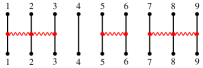
Figure 19: The element $e_{1}e_{2}e_{5}e_{7}e_{8}$ in $\mathcal{C}_{9}$.

For every nonnegative integers $r\leq s$, the $(r,s)$–shift of a set partition $\mathbf{I}\in\mathfrak{C}_{n}$ is the collection

$$\mathbf{I}[r,s]=\{B[r,s]\mid B\in\mathbf{I}\},\quad\text{where}\quad B[r,s]=\{b+r\mid b\in B,\,b\leq n\}\cup\{b+s\mid b\in B,\,b>n\}.$$

Note that coarsening is invariant under shifts, that is, $\mathbf{I}\preceq\mathbf{J}$ if and only if $\mathbf{I}[r,s]\preceq\mathbf{J}[r,s]$.

Given $(\mathbf{I},\mathbf{J})\in\mathfrak{C}_{m}\times\mathfrak{C}_{n}$, the over product of $\mathbf{I}$ with $\mathbf{J}$ is the collection $\mathbf{I}/\mathbf{J}=\mathbf{I}[0,n]\cup\mathbf{J}[m,2m]$. Observe that $\mathbf{I}/\mathbf{J}$ is a set partition of $[2(m+n)]$. See Figure 20.

$$\vbox{\hbox{\includegraphics{pics/014.pdf}}}\kern 4.49997pt/\kern 4.49997pt\vbox{\hbox{\includegraphics{pics/015.pdf}}}\kern 5.50003pt=\kern 4.49997pt\vbox{\hbox{\includegraphics{pics/016.pdf}}}$$

Figure 20: Over product of two set partitions.

We say that $\mathbf{I}\in\mathfrak{C}_{n}$ is $r$–separable for some $r\in[n-1]$ if there is $(\mathbf{J},\mathbf{K})\in\mathfrak{C}_{r}\times\mathfrak{C}_{n-r}$ such that $\mathbf{I}=\mathbf{J}/\mathbf{K}$. Given $\mu=(\mu_{1},\ldots,\mu_{k})\in\mathcal{C}_{n}$, we say that $\mathbf{I}$ is a $\mu$–partition if it is $(\mu_{1}+\cdots+\mu_{i})$–separable for all $i\in[k-1]$. See Figure 21. Note that if $\mathbf{I}$ is a $\mu$–partition, then it is a $\mu^{\prime}$–partition for all composition $\mu^{\prime}\succeq\mu$. Observe that the over product $/$ defines a semigroup structure on $\mathfrak{C}=\bigsqcup_{m\geq 1}\mathfrak{C}_{m}$. Thus, if $\mathbf{I}$ is a $\mu$–partition with $\mu=(\mu_{1},\ldots,\mu_{k})$, then, for each $i\in[k]$, there are $\tilde{\mathbf{I}}_{i}\in\mathfrak{C}_{m_{i}}$ with $m_{i}=\mu_{1}+\cdots+\mu_{i}$ such that $\mathbf{I}=\tilde{\mathbf{I}}_{1}/\cdots/\tilde{\mathbf{I}}_{k}$. This decomposition is unique when $k$ is maximal and, in this case, it is called the boxed decomposition of $\mathbf{I}$.

Figure 21: A $(4,2,3)$–partition of $[18]$.

For every $\mu\in\mathcal{C}_{n}$, there is a unique boxed set partition that is a $\mu$–partition and is not a $\mu^{\prime}$–partition for all $\mu^{\prime}\prec\mu$. This one is called the $u$–boxed partition and is denoted by $b_{\mu}$. For example, the $(3,1,2,3)$–boxed partition of $[18]$ is the one in Figure 16. Conversely, every boxed set partition $\mathbf{I}=(I_{1},\ldots,I_{k})$ is the $u$–boxed partition defined by $\mu=(\frac{|I_{1}|}{2},\ldots,\frac{|I_{k}|}{2})$. This defines the isomorphism of boxed set partitions with $\mathcal{C}_{n}$.

Proposition 4.1.

For every composition $\mu=(\mu_{1},\ldots,\mu_{k})\in\mathcal{C}_{n}$, there are $\mathfrak{b}_{2\mu_{1}}\cdots\mathfrak{b}_{2\mu_{k}}$ $\mu$–partitions.

Proof.

It is a consequence of the fact that $\mathbf{I}$ is a $\mu$–partition if and only if $\mathbf{I}\preceq b_{\mu}$. ∎

See Figure 22 for an example.

$$\begin{array}[]{c}\vbox{\hbox{\includegraphics[scale={0.9}]{pics/018.pdf}}}\quad\vbox{\hbox{\includegraphics[scale={0.9}]{pics/019.pdf}}}\quad\vbox{\hbox{\includegraphics[scale={0.9}]{pics/020.pdf}}}\quad\vbox{\hbox{\includegraphics[scale={0.9}]{pics/021.pdf}}}\quad\vbox{\hbox{\includegraphics[scale={0.9}]{pics/022.pdf}}}\quad\vbox{\hbox{\includegraphics[scale={0.9}]{pics/023.pdf}}}\quad\vbox{\hbox{\includegraphics[scale={0.9}]{pics/024.pdf}}}\quad\vbox{\hbox{\includegraphics[scale={0.9}]{pics/025.pdf}}}\quad\vbox{\hbox{\includegraphics[scale={0.9}]{pics/026.pdf}}}\quad\vbox{\hbox{\includegraphics[scale={0.9}]{pics/027.pdf}}}\\[19.91684pt] \vbox{\hbox{\includegraphics[scale={0.9}]{pics/028.pdf}}}\quad\vbox{\hbox{\includegraphics[scale={0.9}]{pics/029.pdf}}}\quad\vbox{\hbox{\includegraphics[scale={0.9}]{pics/030.pdf}}}\quad\vbox{\hbox{\includegraphics[scale={0.9}]{pics/031.pdf}}}\quad\vbox{\hbox{\includegraphics[scale={0.9}]{pics/032.pdf}}}\quad\vbox{\hbox{\includegraphics[scale={0.9}]{pics/033.pdf}}}\quad\vbox{\hbox{\includegraphics[scale={0.9}]{pics/034.pdf}}}\quad\vbox{\hbox{\includegraphics[scale={0.9}]{pics/035.pdf}}}\quad\vbox{\hbox{\includegraphics[scale={0.9}]{pics/036.pdf}}}\quad\vbox{\hbox{\includegraphics[scale={0.9}]{pics/037.pdf}}}\\[19.91684pt] \vbox{\hbox{\includegraphics[scale={0.9}]{pics/038.pdf}}}\quad\vbox{\hbox{\includegraphics[scale={0.9}]{pics/039.pdf}}}\quad\vbox{\hbox{\includegraphics[scale={0.9}]{pics/040.pdf}}}\quad\vbox{\hbox{\includegraphics[scale={0.9}]{pics/041.pdf}}}\quad\vbox{\hbox{\includegraphics[scale={0.9}]{pics/042.pdf}}}\quad\vbox{\hbox{\includegraphics[scale={0.9}]{pics/043.pdf}}}\quad\vbox{\hbox{\includegraphics[scale={0.9}]{pics/044.pdf}}}\quad\vbox{\hbox{\includegraphics[scale={0.9}]{pics/045.pdf}}}\quad\vbox{\hbox{\includegraphics[scale={0.9}]{pics/046.pdf}}}\quad\vbox{\hbox{\includegraphics[scale={0.9}]{pics/047.pdf}}}\end{array}$$

Figure 22: The $(2,1)$–partitions of $[6]$.

The boxed ramified monoid of a submonoid $M$ of $\mathfrak{C}_{n}$ is the submonoid $\mathcal{BR}(M)$ of $\mathcal{R}(M)$ formed by the ramified partitions $(\mathbf{I},\mathbf{J})$ such that $\mathbf{I}\in M$ and $\mathbf{J}$ is boxed [2, Cf. Definition 55]. See Figure 23.

$$\begin{array}[]{c}\left(\vbox{\hbox{\includegraphics{pics/010.pdf}}}\,\,\,\,,\,\,\,\vbox{\hbox{\includegraphics{pics/011.pdf}}}\right)\\[28.45274pt] \vbox{\hbox{\includegraphics{pics/012.pdf}}}\quad=\quad\vbox{\hbox{\includegraphics{pics/013.pdf}}}\end{array}$$

Figure 23: A ramified partition in $\mathcal{BR}(\mathfrak{C}_{n})$.

Remark 4.2 (Embedding).

Observe that the map $\mathbf{I}\mapsto(\mathbf{I},\mathbf{I})$ is an embedding of $M$ into $\mathcal{BR}(M)$ only if $M$ is formed by boxed set partitions. In particular, $b\mathfrak{C}_{n}$ embeds into $\mathcal{BR}(b\mathfrak{C}_{n})$ via this identification.

On the other hand, as $b_{i}^{2}=b_{i}$ for all $i\in[n-1]$, then, for each $g,h\in\mathcal{BR}(M)$, we have $gh=1$ if and only if $g=h=1$. Therefore $s\mathcal{BR}(M):=\mathcal{BR}(M)\backslash\{1\}$ is a semigroup. Thus $\mathcal{BR}(M)\cap\mathcal{S}_{n}=\{1\}$, which implies that $s\mathcal{BR}(M)$ is a subsemigroup of the singular part $s\mathcal{R}(M):=\mathcal{R}(M)\backslash\mathcal{S}_{n}$ of $\mathcal{R}(M)$.

Since $e_{i}=(1,b_{i})$ for all $i\in[n-1]$, we have $\mathcal{BR}(M)\cap\mathcal{P}_{n}=\mathcal{C}_{n}$ for all submonoid $M$ of $\mathfrak{C}_{n}$. Now, consider the boxed set partition $b=b_{1}\cdots b_{n-1}$. Observe that $(1,b)=e_{1}\cdots e_{n-1}=:e$. Clearly, the map $\mathbf{I}\mapsto(\mathbf{I},\mathbf{I})e=(\mathbf{I},b)$ defines a semigroup monomorphism, called boxed morphism, from $M$ to $\mathcal{BR}(M)$. Moreover, the image of $M$ under the boxed morphism is a monoid with identity $e$. Indeed, since $b^{2}=b$, we have $(\mathbf{I},b)e=(\mathbf{I},b)(1,b)=(\mathbf{I},b)=(1,b)(\mathbf{I},b)=e(\mathbf{I},b)$ for all $\mathbf{I}\in M$.

Observe that $\mathcal{C}_{n}\subseteq Z(\mathcal{BR}(M))$, indeed since $b\mathfrak{C}_{n}$ is commutative, then $(\mathbf{I},\mathbf{J})e_{i}=(\mathbf{I},\mathbf{J}b_{i})=(\mathbf{I},b_{i}\mathbf{J})=e_{i}(\mathbf{I},\mathbf{J})$ for all $(\mathbf{I},\mathbf{J})\in\mathcal{BR}(M)$ and for all $i\in[n-1]$.

Remark 4.3.

Proposition 4.1 implies that for every boxed set partition $\mathbf{J}=(J_{1},\ldots,J_{k})$, there are $\mathfrak{b}_{|J_{1}|}\cdots\mathfrak{b}_{|J_{k}|}$ ramified partitions $(\mathbf{I},\mathbf{J})$. Indeed, $\mathbf{I}\preceq\mathbf{J}$ if and only if $\mathbf{I}$ is a $(\frac{|J_{1}|}{2},\ldots,\frac{|J_{k}|}{2})$–partition. See Figure 24. Thus,

$$|\mathcal{BR}(\mathfrak{C}_{n})|=\sum_{(J_{1},\ldots,J_{k})}\mathfrak{b}_{|J_{1}|}\cdots\mathfrak{b}_{|J_{k}|}=\sum_{(\mu_{1},\ldots,\mu_{k})}\mathfrak{b}_{2\mu_{1}}\cdots\mathfrak{b}_{2\mu_{k}}=(2,19,271,5373,142923,4945661,\ldots),$$

where $(J_{1},\ldots,J_{k})$ is a boxed set partition of $[2n]$, and $(\mu_{1},\ldots,\mu_{k})$ is a composition of $n$.

$$\begin{array}[]{c}\vbox{\hbox{\includegraphics[scale={0.9}]{pics/048.pdf}}}\quad\vbox{\hbox{\includegraphics[scale={0.9}]{pics/049.pdf}}}\quad\vbox{\hbox{\includegraphics[scale={0.9}]{pics/050.pdf}}}\quad\vbox{\hbox{\includegraphics[scale={0.9}]{pics/051.pdf}}}\quad\vbox{\hbox{\includegraphics[scale={0.9}]{pics/052.pdf}}}\quad\vbox{\hbox{\includegraphics[scale={0.9}]{pics/053.pdf}}}\quad\vbox{\hbox{\includegraphics[scale={0.9}]{pics/054.pdf}}}\quad\vbox{\hbox{\includegraphics[scale={0.9}]{pics/055.pdf}}}\quad\vbox{\hbox{\includegraphics[scale={0.9}]{pics/056.pdf}}}\quad\vbox{\hbox{\includegraphics[scale={0.9}]{pics/057.pdf}}}\\[19.91684pt] \vbox{\hbox{\includegraphics[scale={0.9}]{pics/058.pdf}}}\quad\vbox{\hbox{\includegraphics[scale={0.9}]{pics/059.pdf}}}\quad\vbox{\hbox{\includegraphics[scale={0.9}]{pics/060.pdf}}}\quad\vbox{\hbox{\includegraphics[scale={0.9}]{pics/061.pdf}}}\quad\vbox{\hbox{\includegraphics[scale={0.9}]{pics/062.pdf}}}\quad\vbox{\hbox{\includegraphics[scale={0.9}]{pics/063.pdf}}}\quad\vbox{\hbox{\includegraphics[scale={0.9}]{pics/064.pdf}}}\quad\vbox{\hbox{\includegraphics[scale={0.9}]{pics/065.pdf}}}\quad\vbox{\hbox{\includegraphics[scale={0.9}]{pics/066.pdf}}}\quad\vbox{\hbox{\includegraphics[scale={0.9}]{pics/067.pdf}}}\\[19.91684pt] \vbox{\hbox{\includegraphics[scale={0.9}]{pics/068.pdf}}}\quad\vbox{\hbox{\includegraphics[scale={0.9}]{pics/069.pdf}}}\quad\vbox{\hbox{\includegraphics[scale={0.9}]{pics/070.pdf}}}\quad\vbox{\hbox{\includegraphics[scale={0.9}]{pics/071.pdf}}}\quad\vbox{\hbox{\includegraphics[scale={0.9}]{pics/072.pdf}}}\quad\vbox{\hbox{\includegraphics[scale={0.9}]{pics/073.pdf}}}\quad\vbox{\hbox{\includegraphics[scale={0.9}]{pics/074.pdf}}}\quad\vbox{\hbox{\includegraphics[scale={0.9}]{pics/075.pdf}}}\quad\vbox{\hbox{\includegraphics[scale={0.9}]{pics/076.pdf}}}\quad\vbox{\hbox{\includegraphics[scale={0.9}]{pics/077.pdf}}}\end{array}$$

Figure 24: The ramified partitions $(I,b_{1})$ of $[6]$.

As coarsening is invariant under shifts, then $\mathbf{I}\preceq\mathbf{J}$ and $\mathbf{H}\preceq\mathbf{K}$ implies $\mathbf{I}/\mathbf{H}\preceq\mathbf{J}/\mathbf{K}$, hence the over product given by $(\mathbf{I},\mathbf{J})/(\mathbf{H},\mathbf{K})=(\mathbf{I}/\mathbf{H},\mathbf{J}/\mathbf{K})$ defines a semigroup structure on $\mathcal{R}(\mathfrak{C})=\bigsqcup_{m\geq 1}\mathcal{R}(\mathfrak{C}_{m})$.

5 The tied–boxed Hecke algebra

In this section we introduce the tied–boxed Hecke algebra by means generators and relations. Then, we study its representation theory and give a cellular basis for it (Subsection 5.1). Further, we show a diagrammatic realization through the boxed ramified monoid of the symmetric group (Subsection 5.2). Additionally, we study the singular part of the ramified symmetric monoid (Subsection 5.3).

For every positive integer $n$, the tied–boxed Hecke algebra $bH_{n}(q)$ is the $\mathbb{S}$–algebra presented by generators $e_{1},\ldots,e_{n-1}$ satisfying (3.1), and generators $z_{1},\ldots,z_{n-1}$, subject to the following relations:

(5.1) $$z_{i}z_{j}z_{i}=z_{j}z_{i}z_{j},\quad|i-j|=1;\qquad z_{i}z_{j}=z_{j}z_{i},\quad|i-j|>1;$$

(5.2) $$e_{i}z_{i}=z_{i};\qquad e_{i}z_{j}=z_{j}e_{i};$$

(5.3) $$z_{i}^{2}=e_{i}+(q-q^{-1})z_{i}.$$

5.1 Representation theory

Here we study the representation theory of the tied–boxed Hecke algebra. In particular, we get the dimension of $bH_{n}(q)$ (Theorem 5.4) and show that it can be embedded into the algebra of braids and ties (Corollary 5.5). Furthermore, we give a cell datum for $bH_{n}(q)$ and show that it is cellular (Theorem 5.10).

Proposition 5.1.

There is a homomorphism of $\mathbb{S}$–algebras $\iota_{1}:bH_{n}(q)\to\mathcal{E}_{n}(q)$ satisfying $\iota_{1}(e_{i})=e_{i}$ and $\iota_{1}(z_{i})=e_{i}g_{i}$.

Proof.

We need to show that $\iota_{1}(e_{i})$ and $\iota_{1}(z_{i})$ satisfy the defining relations of $bH_{n}(q)$. Relations in (3.1) are directly verified from the definition. The second relation in (5.1) and the first one in (5.2) are consequences of (3.1) and (3.2). To prove the first relation in (5.1) and the second one in (5.2) we will use many times (3.4) and the commutativity relations:

(5.4) $$z_{i}z_{j}z_{i}=e_{i}g_{i}e_{j}g_{j}e_{i}g_{i}=g_{i}(e_{i}e_{j}g_{j})e_{i}g_{i}=g_{i}g_{j}e_{i}e_{j}e_{i}g_{i}=g_{i}g_{j}e_{i}(e_{j}e_{i}g_{i})=g_{i}g_{j}e_{i}g_{i}e_{j}e_{i}=g_{i}g_{j}g_{i}e_{i}e_{j}e_{i}.$$

The first relation in (5.1) is concluded by using the braid relation in (3.2) and the inverse process of (5.4). The second relation in (5.2) is a direct computation, as we show next

$$e_{i}z_{j}=e_{i}e_{j}g_{j}=g_{j}e_{i}e_{j}=g_{j}e_{j}e_{i}=e_{j}g_{j}e_{i}=z_{j}e_{i}.$$

Finally, the quadratic relation in (5.3) is proved as follows

$$z_{i}^{2}=(e_{i}g_{i})^{2}=e_{i}g_{i}^{2}=e_{i}(1+(q-q^{-1})e_{i}g_{i})=e_{i}+(q-q^{-1})e_{i}g_{i}=e_{i}+(q-q^{-1})z_{i}.$$

∎

To study the algebra $bH_{n}(q)$, we will use an adaptation of the element $E_{\mathbf{I}}$ in (3.10). This modification makes sense in $bH_{n}(q)$ only if $\mathbf{I}$ is a linear set partition. To be more precise, for $\mathbf{I}=\{I_{1},\ldots,I_{r}\}\in\mathcal{LP}_{n}$, set

(5.5) $$\operatorname{E}_{\mathbf{I}}=\prod_{i=1}^{r}E_{I_{i}}\,=\prod_{i\,\sim_{\mathbf{I}}\,(i+1)}e_{i}.$$

Lemma 5.2.

The algebra $bH_{n}(q)$ is generated, as an $\mathbb{S}$–module, by $\mathcal{G}_{n}:=\{\operatorname{E}_{\mathbf{I}}z_{w}\mid\mathbf{I}\in\mathcal{LP}_{n},\,w\in\mathcal{S}_{\|\mathbf{I}\|}\}$.

Proof.

From (5.2) we get that each word $x$ in the generators $e_{i}$ and $h_{i}$ can be written as $e_{i_{1}}\cdots e_{i_{r}}z_{j_{1}}\cdots z_{j_{s}}$. Moreover, from (5.2) and (5.5) we can choose the maximal $\mathbf{I}\in\mathcal{LP}_{n}$ such that $\operatorname{E}_{\mathbf{I}}x=x$, that is, if $\mathbf{J}$ is another linear set partition satisfying this condition, then $\mathbf{J}\preceq\mathbf{I}$. Thus, $x$ can be rewritten as $x=\operatorname{E}_{\mathbf{I}}\mathbf{z}=\operatorname{E}_{\mathbf{I}}z_{j_{1}}\cdots z_{j_{r}}$, where $j_{i}\sim_{\mathbf{I}}(j_{i}+1)$ for all $i\in[r]$. Observe that, under multiplication by the respectively $e_{i}$’s, the generators $h_{i}$ satisfy the defining relations of the Hecke algebra. In fact, we have $e_{i}z_{i}^{2}=e_{i}(e_{i}+(q-q^{-1})z_{i})=e_{i}(1+(q-q^{-1})z_{i})$. This implies that $x$ is a linear combination of $\operatorname{E}_{\mathbf{I}}z_{w}$ with $w\in\mathcal{S}_{\|\mathbf{I}\|}$ a reduced expression. ∎

Lemma 5.3.

Let $\mathbf{I}\in\mathcal{LP}_{n}$, and let $w\in S_{\|\mathbf{I}\|}$. Then $\operatorname{E}_{\mathbf{I}}z_{w}$ is mapped to $E_{\mathbf{I}}g_{w}$ under the homomorphism $\iota_{1}$.

Proof.

Let $s_{i_{1}}\cdots s_{i_{r}}$ be a reduced expression of $w$. Then

(5.6) $$\iota_{1}(\operatorname{E}_{\mathbf{I}}z_{w})=E_{\mathbf{I}}\iota_{1}(z_{i_{1}}\cdots z_{i_{r}})=E_{\mathbf{I}}e_{i_{1}}g_{i_{1}}\cdots e_{i_{r}}g_{i_{r}}.$$

Now, observe that $E_{\mathbf{I}}e_{i_{j}}g_{i_{j}}=E_{\mathbf{I}}g_{i_{j}}=g_{i_{j}}E_{\mathbf{I}s_{j}}=g_{i_{j}}E_{\mathbf{I}}$ because $i_{j}\sim_{\mathbf{I}}(i_{j}+1)$ for all $j\in[r]$. By using this observation on the last equality of (5.6), we obtain

$$E_{\mathbf{I}}e_{i_{1}}g_{i_{1}}\cdots e_{i_{r}}g_{i_{r}}=g_{i_{1}}\cdots g_{i_{r}}E_{\mathbf{I}}=g_{w}E_{\mathbf{I}}=E_{\mathbf{I}w}g_{w}.$$

The last expression is equal to $E_{\mathbf{I}}g_{w}$ because $w$ belong to the stabilizer of $\mathbf{I}$. This concludes the proof. ∎

Theorem 5.4.

The algebra $bH_{n}(q)$ is a free $\mathbb{S}$–module with basis $\mathcal{G}_{n}$. In particular, we get

$$\dim bH_{n}(q)=\sum_{(\mu_{1},\ldots,\mu_{k})\,\in\,\mathcal{C}_{n}}\mu_{1}!\cdots\mu_{k}!.$$

Proof.

By Lemma 5.2, it is enough to prove that $\mathcal{G}_{n}$ is a linearly independent subset of $bH_{n}(q)$, which is already satisfied because, due to Lemma 5.3, the subset $\iota_{1}(\mathcal{G}_{n})$ is linearly independent in the algebra $\mathcal{E}_{n}(q)$. ∎

Corollary 5.5.

The homomorphism $\iota_{1}:bH_{n}(q)\to\mathcal{E}_{n}(q)$ is an embedding of $\mathbb{S}$–algebras.

Corollary 5.6.

There is a faithful representation $\varphi$ of $bH_{n}(q)$ in $V^{\otimes n}$ given by $e_{i}\mapsto\mathbf{E}_{i}$ and $z_{i}\mapsto\mathbf{E}_{i}\circ\mathbf{G}_{i}$.

Proof.

This representation is immediately given by the composition $\rho\circ\iota_{1}$. The faithfulness of $\varphi$ follows from injectivity of $\rho$ and $\iota_{1}$. ∎

Remark 5.7.

It is known that the algebra of braids and ties $\mathcal{E}_{n}(q)$ can be regarded as a subalgebra of the $d$–modular Yokonuma–Hecke algebra $Y_{n,d}(q)$ [56, 33, 37, 35]. Indeed, $\mathcal{E}_{n}(q)$ is the subalgebra of $Y_{n,d}(q)$ generated by the elements $g_{1},\ldots,g_{n-1}$ together with the idempotents $e_{1},\ldots,e_{n-1}$ defined as follows:

(5.7) $$e_{i}=\frac{1}{d}\sum_{s=0}^{d-1}t_{i}^{s}t_{i+1}^{-s},$$

where $Y_{n,d}(q)$ is the algebra presented by generators $g_{1},\ldots,g_{n-1}$ satisfying (3.2), and generators $t_{1},\ldots,t_{n}$ subject to the following relations [33, 37, 35, 16]:

(5.8) $$t_{i}^{\,d}=1;\qquad t_{i}t_{j}=t_{j}t_{i};\qquad g_{i}t_{j}=t_{s_{i}(j)}g_{i};\qquad g_{i}^{2}=1+(q-q^{-1})e_{i}g_{i}.$$

Thus, due to Corollary 5.5, the tied–boxed Hecke algebra $bH_{n}(q)$ is the subalgebra of $Y_{n,d}(q)$ generated by the idempotents in (5.7), together with the elements $z_{1},\ldots,z_{n-1}$ defined as follows:

$$z_{i}=\frac{1}{d}\sum_{s=0}^{d-1}t_{i}^{s}t_{i+1}^{-s}g_{i}.$$

In what follows we will show that the tied–boxed Hecke algebra $bH_{n}(q)$ is cellular in the sense of Graham–Lerher [25]. Similarly to the $bt$–algebra [19], we first construct an ideal decomposition of $bH_{n}(q)$.

First, we define a Moëbius function on the lattice $(\mathcal{LP}_{n},\preceq)$ as the map $\mu:\mathcal{LP}_{n}\times\mathcal{LP}_{n}\to\Z$ such that

$$\mu(\mathbf{I},\mathbf{J})=\begin{cases}(-1)^{|\mathbf{I}|-|\mathbf{J}|}&\text{if }\mathbf{I}\preceq\mathbf{J},\\ 0&\text{otherwise.}\end{cases}$$

This Moëbius function will allows us to construct a set of orthogonal idempotents on $bH_{n}(q)$, which are a special case of the general construction given in [54, 27].

For each $\mathbf{I}\in\mathcal{LP}_{n}$, we define

$$\mathbb{E}_{\mathbf{I}}=\sum_{\mathbf{J}\supseteq\mathbf{I}}\mu(\mathbf{I},\mathbf{J})E_{\mathbf{J}}.$$

For example, for $n=3$, we have the following idempotents:

$$\begin{array}[]{lcl}\mathbb{E}_{\{\{1\},\{2\},\{3\}\}}&=&\mathbf{E}_{\{\{1\},\{2\},\{3\}\}}-\mathbf{E}_{\{\{1,2\},\{3\}\}}-\mathbf{E}_{\{\{1\},\{2,3\}\}}+\mathbf{E}_{\{\{1,2,3\}\}}=1-e_{1}-e_{2}+e_{1}e_{2},\\ \mathbb{E}_{\{\{1,2\},\{3\}\}}&=&\mathbf{E}_{\{\{1,2\},\{3\}\}}-\mathbf{E}_{\{\{1,2,3\}\}}=e_{1}-e_{1}e_{2},\\ \mathbb{E}_{\{\{1\},\{2,3\}\}}&=&\mathbf{E}_{\{\{1\},\{2,3\}\}}-\mathbf{E}_{\{\{1,2,3\}\}}=e_{2}-e_{1}e_{2},\\ \mathbb{E}_{\{\{1,2,3\}\}}&=&\mathbf{E}_{\{\{1,2,3\}\}}=e_{1}e_{2}.\end{array}$$

Proposition 5.8.

The following properties hold.

1. $\mathcal{I}_{\mathbb{E}}:=\{\mathbb{E}_{\mathbf{I}}\mid\mathbf{I}\in\mathcal{LP}_{n}\}$ is a complete set of central orthogonal idempotent elements of $bH_{n}$.

2. For all $\mathbf{I}\in\mathcal{LP}_{n}$ we have $\mathbb{E}_{\mathbf{I}}\mathbf{E}_{\mathbf{J}}=\begin{cases}\mathbb{E}_{\mathbf{I}}&\text{if }\mathbf{J}\preceq\mathbf{I},\\ 0&\text{otherwise.}\end{cases}$

Proof.

The proof is similar to the one of [19, Proposition 39]. ∎

As an immediate consequence of Proposition 5.8 we obtain that $bH_{n}(q)$ can be decomposed as a direct sum of two–side ideals.

(5.9) $$bH_{n}(q)\simeq\displaystyle\bigoplus_{\mu\in\mathcal{C}_{n}}bH_{n}(q)^{\mu},$$

where $bH_{n}(q)^{\mu}=\mathbb{E}_{\mathbf{I}}bH_{n}(q)$ and $\mathbf{I}$ is the unique linear set partition satisfying $\|\mathbf{I}\|=\mu$. Moreover, every two–side ideal $bH_{n}(q)^{\mu}$ is also a subalgebra of $bH_{n}(q)$.

Corollary 5.9.

Let $\mathbf{I}\in\mathcal{LP}_{n}$ and suppose that $\|\mathbf{I}\|=\mu=(\mu_{1},\ldots,\mu_{k})\in\mathcal{C}_{n}$. Then, the $\mathbb{S}$–linear map

$$\begin{array}[]{ccccc}bH_{n}(q)^{\mu}&\to&H_{\mu}&\simeq&H_{\mu_{1}}\otimes\cdots\otimes H_{\mu_{k}}\\[8.53581pt] \mathbb{E}_{\mathbf{I}}z_{w}&\mapsto&z_{w}=z_{w_{1}}\cdots z_{w_{k}}&\mapsto&z_{w_{1}}\otimes\cdots\otimes z_{w_{k}}\end{array}$$

is an isomorphism of $\mathbb{S}$–algebras. In particular $\dim bH_{n}(q)^{\mu}=\mu_{1}!\cdots\mu_{k}!$.

Proof.

It is enough to note that $bH_{n}(q)^{\mu}$ is a free $\mathbb{S}$–module with $\mathbb{S}$–basis $\{\mathbb{E}_{\mathbf{I}}z_{w}\mid w\in\mathcal{S}_{\mu}\}$, which is obtained by using the linear basis $\{\mathbf{E}_{\mathbf{I}}z_{w}\}$ of $bH_{n}(q)$ together with Proposition 5.8(2). ∎

In virtue of Corollary 5.9, the decomposition in (5.9) can be rewritten as follows:

(5.10) $$bH_{n}(q)\,\,\,\simeq\displaystyle\bigoplus_{(\mu_{1},\ldots,\mu_{k})\in\mathcal{C}_{n}}H_{\mu_{1}}\otimes\cdots\otimes H_{\mu_{k}}.$$

Due to this isomorphism, the representation theory of the algebra $bH_{n}(q)$ is well known. In fact, we can construct a cell datum for $bH_{n}(q)$ as follows:

1. The poset is the set $\mathcal{LP}_{n}$ of linear multipartitions of $n$ together with the usual dominance order of multipartitions, which we will denote by $\triangleright$.

2. For each ${\boldsymbol{\lambda}}\in\mathcal{LP}_{n}$ we consider $T({\boldsymbol{\lambda}})=\{\boldsymbol{\mathfrak{t}}\in\operatorname{Std}({\boldsymbol{\lambda}})\mid\boldsymbol{\mathfrak{t}}\text{ of the initial kind}\}$.

3. The antiautomorphism $*:bH_{n}(q)\to bH_{n}(q)$ is given by $e_{i}^{*}=e_{i}$ and $z_{i}^{*}=z_{i}$.

4. For each pair ${\boldsymbol{\mathfrak{s}}},\boldsymbol{\mathfrak{t}}\in T({\boldsymbol{\lambda}})$, we define

   $$\mathbf{m}_{{\boldsymbol{\mathfrak{s}}}\boldsymbol{\mathfrak{t}}}^{\boldsymbol{\lambda}}=z_{d({\boldsymbol{\mathfrak{s}}})}^{\ast}\mathbf{m}_{\boldsymbol{\lambda}}z_{d(\boldsymbol{\mathfrak{t}})},\quad\text{where}\quad\mathbf{m}_{\boldsymbol{\lambda}}=\mathbb{E}_{\mathbf{I}_{\boldsymbol{\lambda}}}\sum_{w\in\mathcal{S}_{\boldsymbol{\lambda}}}q^{\ell(w)}z_{w}.$$

Theorem 5.10.

The tied–boxed Hecke algebra $bH_{n}(q)$ is cellular with cellular basis:

$$B=\left\{\mathbf{m}_{{\boldsymbol{\mathfrak{s}}}\boldsymbol{\mathfrak{t}}}^{\boldsymbol{\lambda}}\mid{\boldsymbol{\lambda}}\in\mathcal{LP}_{n}\text{ and }{\boldsymbol{\mathfrak{s}}},\boldsymbol{\mathfrak{t}}\in T({\boldsymbol{\lambda}})\right\}.$$

Proof.

Since the Young Hecke algebras $H_{\mu}$ are cellular, see Subsection 2.4.3, the isomorphism in Corollary 5.9 implies that the algebras $bH_{n}(q)^{\mu}$ are cellular as well. Moreover, a cellular basis for $bH_{n}(q)^{\mu}$ is given by

$$B_{\mu}=\left\{\mathbf{m}_{{\boldsymbol{\mathfrak{s}}}\boldsymbol{\mathfrak{t}}}^{\boldsymbol{\lambda}}\mid\operatorname{\textbf{comp}}({\boldsymbol{\lambda}})=\mu\text{ and }{\boldsymbol{\mathfrak{s}}},\boldsymbol{\mathfrak{t}}\in T({\boldsymbol{\lambda}})\right\}.$$

Then, from (5.10), it is immediate that $bH_{n}(q)$ is a free $\mathbb{S}$–module with basis $B=\coprod_{\mu}B_{\mu}$. Before proving that $B$ satisfies the defining conditions of a cellular basis, observe that the elements $\mathbf{m}_{{\boldsymbol{\mathfrak{s}}}\boldsymbol{\mathfrak{t}}}^{\boldsymbol{\lambda}}$ can be decomposed as a product of classical Murphy’s elements. Indeed, if ${\boldsymbol{\mathfrak{s}}}=(\mathfrak{s}_{1},\ldots,\mathfrak{s}_{k})$ and $\boldsymbol{\mathfrak{t}}=(\mathfrak{t}_{1},\ldots,\mathfrak{t}_{k})$ are standard ${\boldsymbol{\lambda}}=(\lambda^{(1)},\ldots,\lambda^{(k)})$ tableaux of the initial kind, then

$$\begin{array}[]{rcl}\mathbf{m}_{{\boldsymbol{\mathfrak{s}}}\boldsymbol{\mathfrak{t}}}^{\boldsymbol{\lambda}}&=&z_{d({\boldsymbol{\mathfrak{s}}})}^{\ast}\left(\mathbb{E}_{\mathbf{I}_{\boldsymbol{\lambda}}}\sum_{w\in\mathcal{S}_{\boldsymbol{\lambda}}}q^{\ell(w)}z_{w}\right)z_{d(\boldsymbol{\mathfrak{t}})},\\[5.69054pt] &=&\mathbb{E}_{\mathbf{I}_{\boldsymbol{\lambda}}}(z_{d(\mathfrak{s}_{1})}\cdots z_{d(\mathfrak{s}_{k})})^{\ast}\cdot(m_{\lambda^{(1)}}\cdots m_{\lambda^{(k)}})\cdot z_{d(\mathfrak{t}_{1})}\cdots z_{d(\mathfrak{t}_{k})},\\[5.69054pt] &=&\mathbb{E}_{\mathbf{I}_{\boldsymbol{\lambda}}}z_{d(\mathfrak{s}_{k})}^{\ast}\cdots z_{d(\mathfrak{s}_{1})}^{*}\cdot(m_{\lambda^{(1)}}\cdots m_{\lambda^{(k)}})\cdot z_{d(\mathfrak{t}_{1})}\cdots z_{d(\mathfrak{t}_{k})}.\end{array}$$

Now, as $z_{d(\mathfrak{s}_{i})}$ and $m_{\lambda^{(j)}}$ belong to different components of the decomposition of $bH_{n}(q)$ in (5.10), we have

(5.11) $$\mathbf{m}_{{\boldsymbol{\mathfrak{s}}}\boldsymbol{\mathfrak{t}}}^{\boldsymbol{\lambda}}=\mathbb{E}_{\mathbf{I}_{\boldsymbol{\lambda}}}(z_{d(\mathfrak{s}_{l})}^{\ast}m_{\lambda^{(1)}}z_{d(\mathfrak{t}_{1})})\cdots(z_{d(\mathfrak{s}_{k})}^{\ast}m_{\lambda^{(k)}}z_{d(\mathfrak{t}_{k})})=\mathbb{E}_{\mathbf{I}_{\boldsymbol{\lambda}}}m^{\lambda^{(1)}}_{\mathfrak{s}_{1}\mathfrak{t}_{1}}\cdots m^{\lambda^{(k)}}_{\mathfrak{s}_{k}\mathfrak{t}_{k}}.$$

Since the factors in the above decomposition commute with each other and $\mathbb{E}_{\mathbf{I}_{\boldsymbol{\lambda}}}$ is invariant under $\ast$ (it is immediate from the definitions), we have

$$\left(\mathbf{m}_{{\boldsymbol{\mathfrak{s}}}\boldsymbol{\mathfrak{t}}}^{\boldsymbol{\lambda}}\right)^{\ast}=\mathbb{E}_{\mathbf{I}_{\boldsymbol{\lambda}}}^{\ast}\left(m^{\lambda^{(1)}}_{\mathfrak{s}_{1}\mathfrak{t}_{1}}\right)^{\ast}\cdots\left(m^{\lambda^{(k)}}_{\mathfrak{s}_{k}\mathfrak{t}_{k}}\right)^{\ast}=\mathbb{E}_{\mathbf{I}_{\boldsymbol{\lambda}}}m^{\lambda^{(1)}}_{\mathfrak{t}_{1}\mathfrak{s}_{1}}\cdots m^{\lambda^{(k)}}_{\mathfrak{t}_{k}\mathfrak{s}_{k}}=\mathbf{m}_{\boldsymbol{\mathfrak{t}}{\boldsymbol{\mathfrak{s}}}}^{\boldsymbol{\lambda}}.$$

To prove Condition (ii) it is enough to show that it holds for the cases when $a=e_{i}$ and $a=z_{j}$. The case $a=e_{i}$ is trivial because $\mathbb{E}_{\mathbf{I}_{\boldsymbol{\lambda}}}e_{i}=\mathbb{E}_{\mathbf{I}_{\boldsymbol{\lambda}}}$ or $\mathbb{E}_{\mathbf{I}_{\boldsymbol{\lambda}}}e_{i}=0$, see Proposition 5.8. The same occurs for the case when $a=z_{i}$, with $i$ and $i+1$ belong to different blocks of the set partition $\mathbf{I}_{\boldsymbol{\lambda}}$, because $z_{i}=e_{i}z_{i}$. Finally, suppose that $a=z_{i}$, with $i$ and $i+1$ belonging to the block $I_{j}$ of $\mathbf{I}_{\boldsymbol{\lambda}}$. Then,

$$\mathbf{m}_{{\boldsymbol{\mathfrak{s}}}\boldsymbol{\mathfrak{t}}}^{\boldsymbol{\lambda}}z_{i}=\left(\mathbb{E}_{\mathbf{I}_{\boldsymbol{\lambda}}}m^{\lambda^{(1)}}_{\mathfrak{s}_{1}\mathfrak{t}_{1}}\cdots m^{\lambda^{(j)}}_{\mathfrak{s}_{j}\mathfrak{t}_{j}}\cdots m^{\lambda^{(k)}}_{\mathfrak{s}_{k}\mathfrak{t}_{k}}\right)z_{i}=\mathbb{E}_{\mathbf{I}_{\boldsymbol{\lambda}}}m^{\lambda^{(1)}}_{\mathfrak{s}_{1}\mathfrak{t}_{1}}\cdots\left(m^{\lambda^{(j)}}_{\mathfrak{s}_{j}\mathfrak{t}_{j}}z_{i}\right)\cdots m^{\lambda^{(k)}}_{\mathfrak{s}_{k}\mathfrak{t}_{k}}.$$

By applying Condition (ii) in the factor $m^{\lambda^{(j)}}_{\mathfrak{s}_{j}\mathfrak{t}_{j}}h_{i}$, we obtain

(5.12) $$\mathbf{m}_{{\boldsymbol{\mathfrak{s}}}\boldsymbol{\mathfrak{t}}}^{\boldsymbol{\lambda}}z_{i}=\sum_{\mathfrak{v}_{j}\in\operatorname{Std}(\lambda^{(j)})}r_{\mathfrak{v}_{j}}\mathbb{E}_{\mathbf{I}_{\boldsymbol{\lambda}}}m^{\lambda^{(1)}}_{\mathfrak{s}_{1}\mathfrak{t}_{1}}\cdots m^{\lambda^{(j)}}_{\mathfrak{s}_{j}\mathfrak{v}_{j}}\cdots m^{\lambda^{(k)}}_{\mathfrak{s}_{k}\mathfrak{t}_{k}}\quad\mod{H_{n_{j}}^{\lambda^{(j)}}}$$

where $n_{j}$ is the size of $\lambda^{(j)}$. Note that if $\mu\triangleright\lambda^{(j)}$, then ${\boldsymbol{\mu}}=(\lambda^{(1)},\ldots,\mu,\ldots\lambda^{(k)})\triangleright(\lambda^{(1)},\ldots,\lambda^{(j)},\lambda^{(k)})={\boldsymbol{\lambda}}$. Thus, by using the inverse process of the decomposition in (5.11), the equality (5.12) can be rewritten as

$$\mathbf{m}_{{\boldsymbol{\mathfrak{s}}}\boldsymbol{\mathfrak{t}}}^{\boldsymbol{\lambda}}z_{i}=\sum_{\boldsymbol{\mathfrak{v}}_{j}\in\operatorname{Std}({\boldsymbol{\lambda}})}r_{\boldsymbol{\mathfrak{v}}_{j}}\mathbf{m}_{{\boldsymbol{\mathfrak{s}}}\boldsymbol{\mathfrak{v}}_{j}}^{\boldsymbol{\lambda}}\mod{bH_{n}^{\boldsymbol{\lambda}}},$$

where $\boldsymbol{\mathfrak{v}}_{j}=(\mathfrak{t}_{1},\ldots,\mathfrak{v}_{j},\ldots,\mathfrak{t}_{k})$. This concludes the proof. ∎

Remark 5.11.

Let $\mu\in\mathcal{C}_{n}$ and suppose that $\alpha$ is the partition of $n$ obtained by reordering the parts of $\mu$. Then, the embedding $\iota_{1}:bH_{n}(q)\hookrightarrow\mathcal{E}_{n}(q)$ induces an embedding $\iota_{1}^{\mu}:bH_{n}(q)^{\mu}\hookrightarrow\mathcal{E}_{n}(q)^{\alpha}$, which is compatible with the cell structure of these $\mathbb{S}$–algebras. Indeed, $\iota_{1}^{\mu}$ sends the basis element $\mathbf{m}_{{\boldsymbol{\mathfrak{s}}}\boldsymbol{\mathfrak{t}}}^{\boldsymbol{\lambda}}$ of $bH_{n}(q)^{\mu}$ to the basis element $m_{\mathbbm{s}\mathbbm{t}}^{\Lambda}$ of $\mathcal{E}_{n}(q)^{\alpha}$ whose indexes we will explain below.

First, $\Lambda$ is the pair of multipartitions $({\boldsymbol{\lambda}}^{\operatorname{ord}}\mid{\boldsymbol{\mu}})$, where ${\boldsymbol{\lambda}}^{\operatorname{ord}}$ is the increasing multipartition obtained by reordering the parts of ${\boldsymbol{\lambda}}=(\lambda^{(1)},\ldots,\lambda^{(k)})$ and ${\boldsymbol{\mu}}=((1^{m_{1}}),\ldots,(1^{m_{l}}))$, where $m_{i}$ are the multiplicities of equal $\lambda^{(i)}$’s in ${\boldsymbol{\lambda}}^{\operatorname{ord}}$. On the other hand, $\mathbbm{s}$ (resp. $\mathbbm{t}$) is the standard $\Lambda$–tableau $({\boldsymbol{\mathfrak{s}}}^{\operatorname{ord}}\mid\boldsymbol{\mathfrak{t}}^{\boldsymbol{\mu}})$ (resp. $(\boldsymbol{\mathfrak{t}}^{\operatorname{ord}}\mid\boldsymbol{\mathfrak{t}}^{\boldsymbol{\mu}})$), where ${\boldsymbol{\mathfrak{s}}}^{\operatorname{ord}}$ (resp. $\boldsymbol{\mathfrak{t}}^{\operatorname{ord}}$) is the increasing ${\boldsymbol{\lambda}}^{\operatorname{ord}}$–multitableau obtained by reordering the parts of ${\boldsymbol{\mathfrak{s}}}$ (resp. $\boldsymbol{\mathfrak{t}}$). See Figure 25 for an example.

$$\begin{array}[]{c}\left(\left(\scalebox{0.84}{\ytableausetup{boxsize=1.3em,centertableaux}\ytableaushort{45}}\,,\,\scalebox{0.84}{\ytableausetup{boxsize=1.3em,centertableaux}\ytableaushort{9{10}}}\,,\,\scalebox{0.84}{\ytableausetup{boxsize=1.3em,centertableaux}\ytableaushort{{11}{12}}}\,,\,\scalebox{0.84}{\ytableausetup{boxsize=1.3em,centertableaux}\ytableaushort{12,3}}\,,\,\scalebox{0.84}{\ytableausetup{boxsize=1.3em,centertableaux}\ytableaushort{67,8}}\,,\,\scalebox{0.84}{\ytableausetup{boxsize=1.3em,centertableaux}\ytableaushort{{13}{14}{15}}}\right)\Bigg{|}\left(\,\,\scalebox{0.84}{\ytableausetup{boxsize=1.3em,centertableaux}\ytableaushort{1,2,3}}\,,\,\scalebox{0.84}{\ytableausetup{boxsize=1.3em,centertableaux}\ytableaushort{4,5}}\,,\,\scalebox{0.84}{\ytableausetup{boxsize=1.3em,centertableaux}\ytableaushort{6}}\right)\right)\\[22.76228pt] {\boldsymbol{\mathfrak{s}}}=\left(\,\scalebox{0.84}{\ytableausetup{boxsize=1.3em,centertableaux}\ytableaushort{12,3}}\,,\,\scalebox{0.84}{\ytableausetup{boxsize=1.3em,centertableaux}\ytableaushort{45}}\,,\,\scalebox{0.84}{\ytableausetup{boxsize=1.3em,centertableaux}\ytableaushort{67,8}}\,,\,\scalebox{0.84}{\ytableausetup{boxsize=1.3em,centertableaux}\ytableaushort{9{10}}}\,,\,\scalebox{0.84}{\ytableausetup{boxsize=1.3em,centertableaux}\ytableaushort{{11}{12}}}\,,\,\scalebox{0.84}{\ytableausetup{boxsize=1.3em,centertableaux}\ytableaushort{{13}{14}{15}}}\right)\end{array}$$

Figure 25: The $\Lambda$–tableaux associated to the multitableau ${\boldsymbol{\mathfrak{s}}}$.

5.2 Diagrammatic realization of $bH_{n}(q)$

Here we study the boxed ramified monoid associated with the symmetric group, $\mathcal{BR}(\mathcal{S}_{n})$, which can be regarded as a basis for the algebra $bH_{n}(q)$. Specifically, we get that $bH_{n}(q)$ is a $q$–deformation of the monoid algebra generated by $\mathcal{BR}(\mathcal{S}_{n})$ (Theorem 5.13), providing $bH_{n}(q)$ with a structure of diagram algebra. Also, we show that the center of $\mathcal{BR}(\mathcal{S}_{n})$ coincides with the monoid of compositions of $n$ (Proposition 5.16).

It is well known that $|\mathcal{S}_{m}|=m!$ for all integer $m\geq 1$ [29, A356634]. So, similarly as it was done in Proposition 4.1 and Remark 4.3, we have

$$|\mathcal{BR}(\mathcal{S}_{n})|=\sum_{(\mu_{1},\ldots,\mu_{k})}\mu_{1}!\cdots\mu_{k}!=(1,3,11,47,231,1303,8431,62391,524495,4960775,\ldots),$$

where $(\mu_{1},\ldots,\mu_{k})$ is a composition of $n$. See [29, A051296].

For each $i\in[n-1]$, define $z_{i}$ to be the ramified partition $e_{i}s_{i}$ in $\mathcal{R}(\mathcal{S}_{n})$, which is represented as in Figure 26. Due to the relations that define $\mathcal{R}(S_{n})$, the elements $z_{i}$ satisfy the following relations:

(5.13) $$z_{i}z_{j}z_{i}=z_{j}z_{i}z_{j},\quad|i-j|=1;\qquad z_{i}z_{j}=z_{j}z_{i},\quad|i-j|>1;\qquad e_{i}z_{j}=z_{j}e_{i};$$

(5.14) $$z_{i}^{2}=e_{i};\qquad e_{i}z_{i}=z_{i}.$$

$$\begin{array}[]{c}\left(\vbox{\hbox{\includegraphics{pics/002.pdf}}}\cdots\vbox{\hbox{\includegraphics{pics/078.pdf}}}\,\cdots\vbox{\hbox{\includegraphics{pics/002.pdf}}}\,\,\,\,,\,\,\,\vbox{\hbox{\includegraphics{pics/002.pdf}}}\cdots\vbox{\hbox{\includegraphics{pics/079.pdf}}}\,\cdots\vbox{\hbox{\includegraphics{pics/002.pdf}}}\right)\\[28.45274pt] \vbox{\hbox{\includegraphics{pics/002.pdf}}}\cdots\vbox{\hbox{\includegraphics{pics/080.pdf}}}\,\cdots\vbox{\hbox{\includegraphics{pics/002.pdf}}}\quad=\quad\vbox{\hbox{\includegraphics{pics/002.pdf}}}\cdots\vbox{\hbox{\includegraphics{pics/081.pdf}}}\,\cdots\vbox{\hbox{\includegraphics{pics/002.pdf}}}\end{array}$$

Figure 26: Generator $z_{i}=e_{i}s_{i}$.

$$\begin{array}[]{c}\vbox{\hbox{\includegraphics[scale={0.9}]{pics/096.pdf}}}\,\,\,=\,\vbox{\hbox{\includegraphics[scale={0.9}]{pics/097.pdf}}}\,\,\,=\,\vbox{\hbox{\includegraphics[scale={0.9}]{pics/098.pdf}}}\,\,\,=\,\vbox{\hbox{\includegraphics[scale={0.9}]{pics/099.pdf}}}\,\,\,=\,\vbox{\hbox{\includegraphics[scale={0.9}]{pics/100.pdf}}}\,\,\,=\,\vbox{\hbox{\includegraphics[scale={0.9}]{pics/101.pdf}}}\\[28.45274pt] \vbox{\hbox{\includegraphics[scale={0.9}]{pics/106.pdf}}}\,\,\,=\,\vbox{\hbox{\includegraphics[scale={0.9}]{pics/107.pdf}}}\,\,\,=\,\vbox{\hbox{\includegraphics[scale={0.9}]{pics/108.pdf}}}\,\,\,=\,\vbox{\hbox{\includegraphics[scale={0.9}]{pics/109.pdf}}}\kern 35.00005pt\vbox{\hbox{\includegraphics[scale={0.9}]{pics/110.pdf}}}\,\,\,=\,\vbox{\hbox{\includegraphics[scale={0.9}]{pics/111.pdf}}}\,\,\,=\,\vbox{\hbox{\includegraphics[scale={0.9}]{pics/112.pdf}}}\end{array}$$

Figure 27: Some relations in $\mathcal{BR}(\mathcal{S}_{n})$.

Proposition 5.12.

The monoid $\mathcal{BR}(\mathcal{S}_{n})$ is generated by $e_{1},\ldots,e_{n}$ and $z_{1},\ldots,z_{n-1}$.

Proof.

Let $(I,J)\in\mathcal{BR}(\mathcal{S}_{n})$. We have $(I,J)=(\tilde{I}_{1},\tilde{J}_{1})/\cdots/(\tilde{I}_{k},\tilde{J}_{k})$ with $(\tilde{I}_{i},\tilde{J}_{i})\in\mathcal{R}(\mathfrak{C}_{m_{i}})$ for all $i\in[k]$, where $I=\tilde{I}_{1}/\cdots/\tilde{I}_{k}$, and $J=\tilde{J}_{1}/\cdots/\tilde{J}_{k}$ is the boxed decompositions of $J$. Thus, for each $i\in[k]$, we have $(\tilde{I}_{i},\tilde{J}_{i})=(e_{1}\cdots e_{m_{i}})p_{i}$, where $p_{i}\in\mathcal{S}_{m_{i}}$. In general, if $s=s_{i_{1}}\cdots s_{i_{q}}$ is a permutation in $\mathcal{S}_{m}$, we have $(e_{1}\cdots e_{m})s=(e_{1}\cdots e_{m})s_{i_{1}}\cdots s_{i_{q}}=(e_{1}\cdots e_{m})(e_{i_{1}}s_{i_{1}})\cdots(e_{i_{q}}s_{i_{q}})=(e_{1}\cdots e_{m})z_{i_{1}}\cdots z_{i_{q}}$ because of (5.14). Therefore $\mathcal{BR}(\mathcal{S}_{n})$ is generated by $e_{1},\ldots,e_{n}$, $z_{1},\ldots,z_{n-1}$. ∎

Theorem 5.13.

The monoid $\mathcal{BR}(\mathcal{S}_{n})$ is presented by generators $e_{1},\ldots,e_{n-1}$ satisfying (3.1), and generators $z_{1},\ldots,z_{n-1}$ subject to (5.13) and (5.14).

Proof.

Observe that $\mathcal{C}_{m}\times\mathcal{B}_{n}^{+}$ is presented by generators $e_{1},\ldots,e_{n-1}$ and $\sigma_{1},\ldots,\sigma_{n-1}$ satisfying (3.1) and (2.6) together with the relation $e_{i}\sigma_{j}=\sigma_{j}e_{i}$. So, Proposition 5.12 and (5.13) imply that $\varphi:\mathcal{C}_{n}\times\mathcal{B}_{n}^{+}\to\mathcal{BR}(\mathcal{S}_{n})$ defined by $e_{i}\mapsto e_{i}$ and $\sigma_{i}\mapsto z_{i}$ is an epimorphism. Now, let $K$ be the congruence closure generated by the pairs $(\sigma_{i}^{2},e_{i})$ and $(e_{i}\sigma_{i},\sigma_{i})$ for all $i\in[n-1]$. Observe that $K\subseteq\operatorname{Ker}(\varphi)$ because of (5.14).

Consider $e,e^{\prime}\in\mathcal{C}_{n}$ and $\sigma,\sigma^{\prime}\in\mathcal{B}_{n}^{+}$ such that $\sigma=\sigma_{a_{1}}\cdots\sigma_{a_{p}}$, $\sigma^{\prime}=\sigma_{b_{1}}\cdots\sigma_{b_{q}}$ and $\varphi(e\sigma)=\varphi(e^{\prime}\sigma^{\prime})$. Then, because of (5.14), we have

(5.15) $$\varphi(e\sigma)=ee_{a_{1}}\cdots e_{a_{p}}s_{a_{1}}\cdots s_{a_{p}},\qquad\varphi(e^{\prime}\sigma^{\prime})=e^{\prime}e_{b_{1}}\cdots e_{b_{q}}s_{b_{1}}\cdots s_{b_{p}}.$$

Observe that $e\sigma\equiv_{K}ee_{a_{1}}\cdots e_{a_{p}}\sigma$ and $e^{\prime}\sigma^{\prime}\equiv_{K}e^{\prime}e_{b_{1}}\cdots e_{b_{q}}\sigma^{\prime}$ because $(\sigma_{i}^{2},e_{i})\in K$. On the other hand, since $\mathcal{R}(\mathcal{S}_{n})=\mathcal{P}_{n}\rtimes\mathcal{S}_{n}$, the decompositions of $\varphi(e\sigma)$ and $\varphi(e^{\prime}\sigma^{\prime})$ in (5.15) are unique, hence

$$ee_{a_{1}}\cdots e_{a_{p}}=e^{\prime}e_{b_{1}}\cdots e_{b_{q}},\qquad s_{a_{1}}\cdots s_{a_{p}}=s_{b_{1}}\cdots s_{b_{q}}.$$

Note that each relation of $\mathcal{S}_{n}$ used to get $s_{b_{1}}\cdots s_{b_{q}}$ from $s_{a_{1}}\cdots s_{a_{p}}$ can be translated into a relation of $z_{i}$’s because if $s_{i}$ occurs above then $e_{i}$ occurs as well. Thus $e\sigma\equiv_{K}ee_{a_{1}}\cdots e_{a_{p}}\sigma\equiv_{K}e^{\prime}e_{b_{1}}\cdots e_{b_{q}}\sigma^{\prime}\equiv_{K}e^{\prime}\sigma^{\prime}$, and then $\operatorname{Ker}(\varphi)\subseteq K$. Therefore $\mathcal{BR}(\mathcal{S}_{n})\simeq(\mathcal{C}_{n}\times\mathcal{B}_{n}^{+})/K$, which proves the theorem. ∎

It is immediate from Theorem 5.13 that $bH_{n}(q)$ is a $q$–deformation of the monoid algebra generated by $\mathcal{BR}(S_{n})$. Thus, the algebra $bH_{n}(q)$ inherits the diagram combinatorics of $\mathcal{BR}(\mathcal{S}_{n})$. See Figure 28.

$$\vbox{\hbox{\includegraphics{pics/154.pdf}}}\,\,\,=\,\vbox{\hbox{\includegraphics{pics/155.pdf}}}\,\,+\,\,(q-q^{-1})\!\!\vbox{\hbox{\includegraphics{pics/156.pdf}}}\quad\Leftrightarrow\quad\vbox{\hbox{\includegraphics{pics/157.pdf}}}\,\,\,=\,\vbox{\hbox{\includegraphics{pics/158.pdf}}}\,\,+\,\,(q-q^{-1})\!\!\vbox{\hbox{\includegraphics{pics/159.pdf}}}$$

Figure 28: Relation (5.3) in terms of diagrams.

Remark 5.14.

By using Tietze transformations, and due to the fact that $e_{i}=z_{i}^{2}$, the monoid $\mathcal{BR}(\mathcal{S}_{n})$ can be presented by generators $z_{1},\ldots,z_{n-1}$, subject to the following relations:

$$z_{i}z_{j}z_{i}=z_{j}z_{i}z_{j},\quad|i-j|=1;\qquad z_{i}z_{j}=z_{j}z_{i},\quad|i-j|>1;\qquad z_{i}^{3}=z_{i};\qquad z_{i}^{2}z_{j}^{2}=z_{j}^{2}z_{i}^{2};\qquad z_{i}^{2}z_{j}=z_{j}z_{i}^{2}.$$

Remark 5.15 (Normal form).

As shown in the proofs of Proposition 5.12 and Theorem 5.13, every element $g\in\mathcal{BR}(\mathcal{S}_{n})$ can be uniquely written as $ez$ with $e\in\mathcal{C}_{n}$ and $z=z_{i_{1}}\cdots z_{i_{k}}$, where $es_{i_{1}}\cdots s_{i_{k}}$ is a normal decomposition given by the semidirect product structure of $\mathcal{R}(\mathcal{S}_{n})$. Moreover, as $e$ is formed by blocks, then $g=ze$ as well. See Figure 29.

$$\vbox{\hbox{\includegraphics{pics/149.pdf}}}\quad=\quad\vbox{\hbox{\includegraphics{pics/150.pdf}}}\quad=\quad\vbox{\hbox{\includegraphics{pics/151.pdf}}}\quad=\quad\vbox{\hbox{\includegraphics{pics/152.pdf}}}$$

Figure 29: Normal form of $e_{1}e_{2}e_{3}s_{2}s_{1}s_{3}s_{2}s_{3}=e_{1}e_{2}e_{3}z_{2}z_{1}z_{3}z_{2}z_{3}=z_{2}z_{1}z_{3}z_{2}z_{3}e_{1}e_{2}e_{3}$.

Proposition 5.16.

We have $Z(\mathcal{BR}(\mathcal{S}_{n}))=\mathcal{C}_{n}$ for all $n\geq 3$.

Proof.

Due to Theorem 5.13 and the relations that define $\mathcal{S}_{n}$, we conclude that the map $\phi:\mathcal{BR}(\mathcal{S}_{n})\to\mathcal{S}_{n}$ sending $z_{i}\mapsto s_{i}$ and $e_{i}\mapsto 1$ is a monoid epimorphism. So, $\phi(g)\in Z(\mathcal{S}_{n})=\{1\}$ for all $g\in Z(\mathcal{BR}(\mathcal{S}_{n}))$. Observe that $\phi(\mathcal{C}_{n})=\{1\}$ and $\mathcal{C}_{n}\subseteq\mathcal{BR}(\mathcal{S}_{n})$ as mentioned in Remark 4.2. On the other hand, as each relation in (2.3) can be obtained from one in (5.13) and (5.14), then every element of $\mathcal{BR}(\mathcal{S}_{n})$ can be written as a product $ez$, where $e\in\mathcal{C}_{n}$ and $z=z_{i_{1}}\cdots z_{i_{k}}$ such that $\phi(z)=s_{i_{1}}\cdots s_{i_{k}}$ is a reduced expression in $\mathcal{S}_{n}$. This implies that $\phi(g)=1$ for some $g\in\mathcal{BR}(\mathcal{S}_{n})$ if and only if $g\in\mathcal{C}_{n}$. Therefore $Z(\mathcal{BR}(\mathcal{S}_{n}))=\mathcal{C}_{n}$. ∎

Remark 5.17.

Just as the symmetric group can be obtained by imposing the relations $\sigma_{i}^{2}=1$ in the braid group, the ramified symmetric monoid can be obtained in this manner from the tied braid monoid. It is expected that a monoid playing this role for $\mathcal{BR}(\mathcal{S}_{n})$ is the submonoid $bT\mathcal{B}_{n}$ of $T\mathcal{B}_{n}$ generated by $\tau_{i}:=e_{i}\sigma_{i}$ and $\tilde{\tau}_{i}:=e_{i}\sigma_{i}^{-1}$ for all $i\in[n-1]$, together with $e_{1},\ldots,e_{n-1}$ satisfying (3.1). This submonoid will be called the tied–boxed braid monoid. Observe that, due to (3.20) and (3.21), the generators $\tau_{i}$ and $\tilde{\tau}_{i}$ satisfy the relations below. It is an open problem to check if these relations are sufficient to give a presentation.

$$\tau_{i}\tau_{j}\tau_{i}=\tau_{j}\tau_{i}\tau_{j},\quad\tilde{\tau}_{i}\tilde{\tau}_{j}\tilde{\tau}_{i}=\tilde{\tau}_{j}\tilde{\tau}_{i}\tilde{\tau}_{j},\quad|i-j|=1;$$

$$\tau_{i}\tilde{\tau}_{i}=e_{i}=\tilde{\tau}_{i}\tau_{i};\qquad e_{i}\tau_{j}=\tau_{j}e_{i};\qquad e_{i}\tilde{\tau}_{j}=\tilde{\tau}_{j}e_{i};\qquad e_{i}\tau_{i}=\tau_{i};\qquad e_{i}\tilde{\tau}_{i}=\tilde{\tau}_{i}.$$

5.3 The singular part of $\mathcal{R}(\mathcal{S}_{n})$

As mentioned in Remark 4.2, $\mathcal{BR}(\mathcal{S}_{n})\backslash\{1\}$ is a subsemigroup of the singular part of $\mathcal{R}(\mathcal{S}_{n})$. Hence, the monoid $s\mathcal{R}(\mathcal{S}_{n})^{1}$ can be regarded as an extension of $\mathcal{BR}(\mathcal{S}_{n})$. Here, we study the singular part of the ramified symmetric monoid, in particular we give a presentation for it (Theorem 5.20).

In this subsection, for each $r_{1},\ldots,r_{k}\in[n-1]$ and each $i\in[n]$, we will denote the image of $i$ under the permutation $s_{r_{1}}\cdots s_{r_{k}}$ by $(r_{1}\circ\cdots\circ r_{k})(i)$ instead.

Observe that $s\mathcal{R}(\mathcal{S}_{n})=\{(I,J)\mid I\in\mathcal{S}_{n},\,I\prec J\}$ and $|s\mathcal{R}(\mathcal{S}_{n})|=n!\mathfrak{b}_{n}-n!=n!(\mathfrak{b}_{n}-1)$. See Figure 30.

$$\begin{array}[]{c}\includegraphics[scale={0.9}]{pics/118.pdf}\quad\includegraphics[scale={0.9}]{pics/119.pdf}\quad\includegraphics[scale={0.9}]{pics/120.pdf}\quad\includegraphics[scale={0.9}]{pics/121.pdf}\quad\includegraphics[scale={0.9}]{pics/122.pdf}\quad\includegraphics[scale={0.9}]{pics/123.pdf}\quad\includegraphics[scale={0.9}]{pics/124.pdf}\quad\includegraphics[scale={0.9}]{pics/125.pdf}\\[1.99168pt] \includegraphics[scale={0.9}]{pics/126.pdf}\quad\includegraphics[scale={0.9}]{pics/127.pdf}\quad\includegraphics[scale={0.9}]{pics/128.pdf}\quad\includegraphics[scale={0.9}]{pics/129.pdf}\quad\includegraphics[scale={0.9}]{pics/130.pdf}\quad\includegraphics[scale={0.9}]{pics/131.pdf}\quad\includegraphics[scale={0.9}]{pics/132.pdf}\quad\includegraphics[scale={0.9}]{pics/133.pdf}\\[1.99168pt] \includegraphics[scale={0.9}]{pics/134.pdf}\quad\includegraphics[scale={0.9}]{pics/135.pdf}\quad\includegraphics[scale={0.9}]{pics/136.pdf}\quad\includegraphics[scale={0.9}]{pics/137.pdf}\quad\includegraphics[scale={0.9}]{pics/138.pdf}\quad\includegraphics[scale={0.9}]{pics/139.pdf}\quad\includegraphics[scale={0.9}]{pics/140.pdf}\quad\includegraphics[scale={0.9}]{pics/141.pdf}\end{array}$$

Figure 30: The $24$ elements of $s\mathcal{R}(\mathcal{S}_{3})$.

For each $i,j,r\in[n-1]$ with $j<k$, we define $z^{r}_{i,j}=e_{i,j}s_{r}$. See Figure 31. Note that $z^{i}_{i,i+1}=z_{i}$. Also, there are $\frac{n^{2}(n-1)}{2}$ [29, A006002] of these elements, and each $z_{i,j}^{r}$ belongs to $s\mathcal{R}(\mathcal{S}_{n})$ due to occurrence of $e_{i,j}$.

      

Figure 31: Elements $z^{2}_{1,4}$ and $z^{1}_{2,4}$ in $\mathcal{R}(\mathcal{S}_{n})$.

Proposition 5.18.

The semigroup $s\mathcal{R}(\mathcal{S}_{n})$ is generated by the elements $z^{r}_{i,j}$ and $e_{i,j}$.

Proof.

Since $s\mathcal{R}(\mathcal{S}_{n})$ is a subsemigroup of $\mathcal{R}(S_{n})=\mathcal{P}_{n}\rtimes\mathcal{S}_{n}$, every element $g\in s\mathcal{R}(\mathcal{S}_{n})$ can be uniquely written as a product $es$, where $e\in\mathcal{P}_{n}$ and $s\in\mathcal{S}_{n}$. Let $e_{p_{1},q_{1}}\cdots e_{p_{h},q_{h}}$ be the normal form of $e$ as in [11, Proposition 3.3], and let $s_{r_{1}}\cdots s_{r_{k}}$ be a word of minimal length representing $s$. Then, we have

(5.16) $$g=e_{p_{1},q_{1}}\cdots e_{p_{h},q_{h}}s_{r_{1}}\cdots s_{r_{k}}=e_{p_{2},q_{2}}\cdots e_{p_{h},q_{h}}(e_{\bar{p}_{1},\bar{q}_{1}}s_{r_{1}})\cdots(e_{\bar{p}_{k},\bar{q}_{k}}s_{r_{k}})=e_{p_{2},q_{2}}\cdots e_{p_{h},q_{h}}z_{\bar{p}_{1},\bar{q}_{1}}^{r_{1}}\cdots z_{\bar{p}_{k},\bar{q}_{k}}^{r_{k}},$$

where $e_{\bar{p}_{i},\bar{q}_{i}}=s_{r_{i-1}}\cdots s_{r_{1}}e_{p_{1},q_{1}}s_{r_{1}}\cdots s_{r_{i-1}}$. Therefore $s\mathcal{R}(\mathcal{S}_{n})$ is generated by the elements $z^{r}_{i,j}$ and $e_{i,j}$. ∎

Remark 5.19 (Normal form).

Observe that the word $u=e_{p_{2},q_{2}}\cdots e_{p_{h},q_{h}}z_{\bar{p}_{1},\bar{q}_{1}}^{r_{1}}\cdots z_{\bar{p}_{k},\bar{q}_{k}}^{r_{k}}$ representing the element $g$ in (5.16) is uniquely defined up to the choice of the minimal length word $v=s_{r_{1}}\cdots s_{r_{k}}$. We may assume that $v$ is chosen in some minimal length normal form of $s$. Thus, $u$ will be a normal form for $g$. See Figure 32 for an instance.

$$\vbox{\hbox{\includegraphics{pics/146.pdf}}}\quad\,=\quad\vbox{\hbox{\includegraphics{pics/147.pdf}}}\quad\,=\quad\vbox{\hbox{\includegraphics{pics/148.pdf}}}$$

Figure 32: Normal form of $e_{1,2}e_{2,4}s_{3}s_{1}s_{2}s_{1}=e_{2,4}z_{1,2}^{3}z_{1,2}^{1}z_{1,2}^{2}z_{1,3}^{1}$.

Due to the fact that $\mathcal{R}(\mathcal{S}_{n})=\mathcal{P}_{n}\rtimes\mathcal{S}_{n}$ and the relations that define it, we can show that the generators $z_{i,j}^{r}$ satisfy the following relations:

(5.17) $$z^{r}_{i,j}z^{t}_{r(i),r(j)}z^{r}_{(t\circ r)(i),(t\circ r)(j)}=z^{t}_{i,j}z^{r}_{t(i),t(j)}z^{t}_{(r\circ t)(i),(r\circ t)(j)},\quad|r-t|=1;$$

(5.18) $$z^{r}_{i,j}z^{t}_{r(i),r(j)}=z^{t}_{i,j}z^{r}_{t(i),t(j)},\quad|r-t|>1;$$

(5.19) $$z^{r}_{i,j}z^{r}_{h,k}=e_{i,j}e_{r(h),r(k)};\qquad e_{i,j}z^{r}_{i,j}=z^{r}_{i,j};\qquad z^{r}_{i,j}e_{h,k}=e_{r(h),r(k)}z^{r}_{i,j}.$$

Observe that (5.17) and (5.18) are inherited from the braid relations that the generators $s_{i}$ hold. See Figure 33. Furthermore, (5.19) implies it is enough to consider the generators $z^{r}_{i,j}$ because $e_{i,j}=e_{i,j}^{2}=z^{r}_{i,j}z^{r}_{r(i),r(j)}$.

$$\vbox{\hbox{\includegraphics{pics/142.pdf}}}\quad=\!\quad\vbox{\hbox{\includegraphics{pics/143.pdf}}}\kern 40.00006pt\vbox{\hbox{\includegraphics{pics/144.pdf}}}\quad=\quad\vbox{\hbox{\includegraphics{pics/145.pdf}}}$$

Figure 33: Relations $z^{1}_{2,3}z^{2}_{1,3}z^{1}_{1,2}=z^{2}_{2,3}z^{1}_{2,3}z^{2}_{1,3}$ and $z^{1}_{2,4}z^{2}_{1,4}=z^{2}_{2,4}z^{1}_{2,3}$.

The main goal of this subsection is to prove the following result.

Theorem 5.20.

The semigroup $s\mathcal{R}(\mathcal{S}_{n})$ is presented by generators $e_{i,j}$ satisfying (2.2), and generators $z^{r}_{i,j}$, subject to the relations (5.17) to (5.19).

Remark 5.21.

Observe that $gh,hg\in s\mathcal{R}(\mathcal{S}_{n})$ for all $g\in\mathcal{S}_{n}$ and $h\in s\mathcal{R}(\mathcal{S}_{n})$. Hence $s\mathcal{R}(\mathcal{S}_{n})$ is an ideal of the monoid $\mathcal{R}(\mathcal{S}_{n})$. So, another manner to show a presentation for $s\mathcal{R}(\mathcal{S}_{n})$ can be obtained by applying the Reidemeister–Schreier type rewriting for ideals given in [51, 15].

5.3.1 Proof of Theorem 5.20

Let $S$ be the semigroup presented by generators ${\tt e}_{i,j}$ and ${\tt z}^{r}_{i,j}$ with $r\in[n-1]$ and $i,j\in[n]$ such that $i<j$, subject to the following relations:

(5.20) $${\tt e}_{i,j}^{2}={\tt e}_{i,j},\quad{\tt e}_{i,j}{\tt e}_{r,s}={\tt e}_{r,s}{\tt e}_{i,j},\quad{\tt e}_{i,j}{\tt e}_{i,k}={\tt e}_{i,j}{\tt e}_{j,k}={\tt e}_{i,k}{\tt e}_{j,k};$$

(5.21) $${\tt z}^{r}_{i,j}{\tt z}^{t}_{r(i),r(j)}{\tt z}^{r}_{(t\circ r)(i),(t\circ r)(j)}={\tt z}^{t}_{i,j}{\tt z}^{r}_{t(i),t(j)}{\tt z}^{t}_{(r\circ t)(i),(r\circ t)(j)},\quad|r-t|=1;$$

(5.22) $${\tt z}^{r}_{i,j}{\tt z}^{t}_{r(i),r(j)}={\tt z}^{t}_{i,j}{\tt z}^{r}_{t(i),t(j)},\quad|r-t|>1;$$

(5.23) $${\tt z}^{r}_{i,j}{\tt z}^{r}_{h,k}={\tt e}_{i,j}{\tt e}_{r(h),r(k)};\qquad{\tt e}_{i,j}{\tt z}^{r}_{i,j}={\tt z}^{r}_{i,j};\qquad{\tt z}^{r}_{i,j}{\tt e}_{h,k}={\tt e}_{r(h),r(k)}{\tt z}^{r}_{i,j}.$$

As relations (2.2) and (5.17)–(5.19) hold in $s\mathcal{R}(\mathcal{S}_{n})$, the map $\phi$ sending ${\tt e}_{i,j}\mapsto e_{i,j}$ and ${\tt z}_{i,j}^{r}\mapsto z_{i,j}^{r}$ for all $r\in[n-1]$ and $i,j\in[n]$ with $i<j$, defines a semigroup epimorphism from $S$ to $s\mathcal{R}(\mathcal{S}_{n})$.

Lemma 5.22.

The following relations hold in $S$.

1. ${\tt e}_{i,j}{\tt z}_{h,k}^{r}={\tt e}_{h,k}{\tt z}_{i,j}^{r}$.

2. ${\tt z}^{r}_{i,j}{\tt z}^{t}_{h,k}{\tt z}^{r}_{p,q}={\tt z}^{t}_{i,j}{\tt z}^{r}_{(t\circ r)(h),(t\circ r)(k)}{\tt z}^{t}_{(t\circ r)(p),(t\circ r)(q)}$ if $|r-t|=1$.

3. ${\tt z}_{i,j}^{r}{\tt z}_{h,k}^{t}={\tt z}_{i,j}^{t}{\tt z}_{(t\circ r)(h),(t\circ r)(k)}^{r}$ if $|r-t|>1$.

Proof.

By using (5.23), we show (1) as follows:

$${\tt e}_{i,j}{\tt z}_{h,k}^{r}={\tt e}_{i,j}{\tt e}_{h,k}{\tt z}_{h,k}^{r}={\tt z}^{r}_{i,j}{\tt z}^{r}_{r(h),r(k)}{\tt z}_{h,k}^{r}={\tt z}^{r}_{i,j}{\tt e}_{r(h),r(k)}{\tt e}_{r(h),r(k)}={\tt z}^{r}_{i,j}{\tt e}_{r(h),r(k)}={\tt e}_{h,k}{\tt z}^{r}_{i,j}.$$

To show (2) and (3), we apply (5.21) and (5.22) together with (1) and (5.23), as follows:

$$\begin{array}[]{rcl}{\tt z}^{r}_{i,j}{\tt z}^{t}_{h,k}{\tt z}^{r}_{p,q}&=&{\tt e}_{i,j}^{2}{\tt z}^{r}_{i,j}{\tt z}^{t}_{h,k}{\tt z}^{r}_{p,q},\\ &=&{\tt z}^{r}_{i,j}{\tt e}_{r(i),r(j)}{\tt z}^{t}_{h,k}{\tt e}_{(t\circ r)(i),(t\circ r)(j)}{\tt z}^{r}_{p,q},\\ &=&{\tt z}^{r}_{i,j}{\tt e}_{h,k}{\tt z}^{t}_{r(i),r(j)}{\tt e}_{p,q}{\tt z}^{r}_{(t\circ r)(i),(t\circ r)(j)},\\ &=&{\tt e}_{r(h),r(k)}{\tt e}_{(r\circ t)(p),(r\circ t)(q)}{\tt z}^{r}_{i,j}{\tt z}^{t}_{r(i),r(j)}{\tt z}^{r}_{(t\circ r)(i),(t\circ r)(j)},\\ &=&{\tt e}_{r(h),r(k)}{\tt e}_{(r\circ t)(p),(r\circ t)(q)}{\tt z}^{t}_{i,j}{\tt z}^{r}_{t(i),t(j)}{\tt z}^{t}_{(r\circ t)(i),(r\circ t)(j)},\\ &=&{\tt z}^{t}_{i,j}{\tt e}_{(t\circ r)(h),(t\circ r)(k)}{\tt z}^{r}_{t(i),t(j)}{\tt e}_{(t\circ r)(p),(t\circ r)(q)}{\tt z}^{t}_{(r\circ t)(i),(r\circ t)(j)},\\ &=&{\tt z}^{t}_{i,j}{\tt e}_{t(i),t(j)}{\tt z}^{r}_{(t\circ r)(h),(t\circ r)(k)}{\tt e}_{(r\circ t)(i),(r\circ t)(j)}{\tt z}^{t}_{(t\circ r)(p),(t\circ r)(q)},\\ &=&{\tt e}_{i,j}^{2}{\tt z}^{t}_{i,j}{\tt z}^{r}_{(t\circ r)(h),(t\circ r)(k)}{\tt z}^{t}_{(t\circ r)(p),(t\circ r)(q)},\\ &=&{\tt z}^{t}_{i,j}{\tt z}^{r}_{(t\circ r)(h),(t\circ r)(k)}{\tt z}^{t}_{(t\circ r)(p),(t\circ r)(q)}.\end{array}\begin{array}[]{rcl}{\tt z}_{i,j}^{r}{\tt z}_{h,k}^{t}&=&{\tt e}_{i,j}{\tt z}_{i,j}^{r}{\tt z}_{h,k}^{t},\\ &=&{\tt z}_{i,j}^{r}{\tt e}_{r(i),r(j)}{\tt z}_{h,k}^{t},\\ &=&{\tt z}_{i,j}^{r}{\tt e}_{h,k}{\tt z}_{r(i),r(j)}^{t},\\ &=&{\tt e}_{r(h),r(k)}{\tt z}_{i,j}^{r}{\tt z}_{r(i),r(j)}^{t},\\ &=&{\tt e}_{r(h),r(k)}{\tt z}_{i,j}^{t}{\tt z}_{t(i),t(j)}^{r},\\ &=&{\tt z}_{i,j}^{t}{\tt e}_{(t\circ r)(h),(t\circ r)(k)}{\tt z}_{t(i),t(j)}^{r},\\ &=&{\tt z}_{i,j}^{t}{\tt e}_{t(i),t(j)}{\tt z}_{(t\circ r)(h),(t\circ r)(k)}^{r},\\ &=&{\tt e}_{i,j}{\tt z}_{i,j}^{t}{\tt z}_{(t\circ r)(h),(t\circ r)(k)}^{r},\\ &=&{\tt z}_{i,j}^{t}{\tt z}_{(t\circ r)(h),(t\circ r)(k)}^{r}.\end{array}$$

∎

Parts (2) and (3) of Lemma 5.22 imply that, independently of the subindices, the generators ${\tt z}^{r}_{i,j}$ satisfy the braid relations with respect of their superindices, that is

(5.24) $${\tt z}_{\square}^{r}{\tt z}_{\square}^{t}{\tt z}_{\square}^{r}={\tt z}_{\square}^{t}{\tt z}_{\square}^{r}{\tt z}_{\square}^{t},\quad|i-j|=1;\qquad{\tt z}_{\square}^{r}{\tt z}_{\square}^{t}={\tt z}_{\square}^{t}{\tt z}_{\square}^{r},\quad|i-j|>1;$$

where the square is hiding the subindices of each generator. Similarly, relations in (5.23) can be written as:

(5.25) $${\tt z}_{\square}^{r}{\tt z}_{\square}^{r}={\tt e}_{\square};\qquad{\tt e}_{\square}{\tt z}_{\square}^{r}={\tt z}_{\square}^{r};\qquad{\tt z}_{\square}^{r}{\tt e}_{\square}={\tt e}_{\square}{\tt z}_{\square}^{r};$$

Thus, we obtain the following result.

Corollary 5.23.

The map $\phi_{s}:S\to\mathcal{S}_{n}$ sending ${\tt e}_{i,j}\mapsto 1$ and ${\tt z}_{i,j}^{r}\mapsto s_{r}$ defines a semigroup endomorphism.

Proposition 5.24.

Every element $g\in S$ can be represented by a word in the generators ${\tt e}_{i,j}$ and ${\tt z}_{i,j}^{r}$, such that the word obtained from it when replacing ${\tt e}_{i,j}$ by $e_{i,j}$ and ${\tt z}_{i,j}^{r}$ by $z_{i,j}^{r}$ is a normal form of $\phi(g)$.

Proof.

Due to the third relation in (5.25), every element $g\in S$ can be represented by a word $eu$, where $e$ is a word in the generators ${\tt e}_{i,j}$ and $u$ is a word in the generators ${\tt z}_{i,j}^{r}$. Moreover, because of (5.24) and (5.25), we can assume that $u={\tt z}_{\square}^{r_{1}}\cdots{\tt z}_{\square}^{r_{k}}$ is of minimal length, that is, $\phi_{s}(eu)=s_{r_{1}}\cdots s_{r_{k}}$ is of minimal length. Observe that, by applying (5.25), we have

$$u\equiv(\underbrace{{\tt e}_{\bar{p}_{1},\bar{q}_{1}}\cdots{\tt e}_{\bar{p}_{k},\bar{q}_{k}}}_{e^{\prime}})\underbrace{{\tt z}_{\square}^{r_{1}}\cdots{\tt z}_{\square}^{r_{k}}}_{z},\quad\text{where}\quad{\tt z}_{\square}^{r_{i}}={\tt z}_{p_{i},q_{i}}^{r_{i}},\quad{\tt e}_{\bar{p}_{i},\bar{q}_{i}}={\tt e}_{(r_{1}\circ\cdots\circ r_{i-1})(p_{i}),(r_{1}\circ\cdots\circ r_{i-1})(q_{i})}.$$

Thus $\phi(g)=\phi(ee^{\prime})\phi(z)=\phi(ee^{\prime})\phi_{s}(z)$ because each tie connecting strands in $\phi(z)$ is already occurring in $\phi(ee^{\prime})$. Moreover, due to (5.20), we can assume that $ee^{\prime}$ is written in normal form as in [11, Proposition 3.3]. Finally, by using (1) in Lemma 5.22, the first generator $e_{a_{1},a_{2}}$ of $ee^{\prime}$ can be removed and each generator ${\tt z}^{r_{i}}_{p_{i},q_{i}}$ can be replaced by ${\tt z}^{r_{i}}_{\tilde{p}_{i},\tilde{q}_{i}}$, where $\tilde{p}_{i}=(r_{i-1}\circ\cdots\circ r_{1})(p_{i})$ and $\tilde{q}_{i}=(r_{i-1}\circ\cdots\circ r_{1})(q_{i})$. Thus, the word obtained from $ee^{\prime}z$ when replacing ${\tt e}_{i,j}$ by $e_{i,j}$ and ${\tt z}_{i,j}^{r}$ by $z_{i,j}^{r}$ is a normal form of $\phi(g)$. ∎

Proof of Theorem 5.20.

Let $g,g^{\prime}\in S$ such that $\phi(g)=\phi(g^{\prime})$, and let $u$ be the normal form of $\phi(g)$ as in Remark 5.19. Proposition 5.24 implies both $g,g^{\prime}$ have word representatives in the generators ${\tt e}_{i,j}$ and ${\tt z}_{i,j}^{r}$, which become $u$ when replace ${\tt e}_{i,j}$ by $e_{i,j}$ and ${\tt z}_{i,j}^{r}$ by $z_{i,j}^{r}$. Since $u$ is uniquely defined, these words must be identical. Thus $g=g^{\prime}$. Therefore $\phi$ is an isomorphism. ∎

6 The tied–boxed Temperley–Lieb algebra

In this section, inspired by the quotient of $\mathcal{E}_{n}(q)$ in [53], which in turn was inspired by [28], we introduce the tied–boxed Temperley–Lieb algebra. Then, we give a cellular basis for it (Theorem 6.2) and study its connection with the partition Temperley–Lieb algebra introduced by Juyumaya [36] (Subsection 6.1). Further, we show a diagrammatic realization through the boxed ramified monoid of the Jones monoid (Subsection 6.2). Additionally, we study the boxed ramified monoid of the Brauer monoid (Subsection 6.3).

The tied–boxed Temperley–Lieb algebra $bTL_{n}(q)$ is the quotient of $bH_{n}(q)$ by the two–sided ideal generated by the following Steinberg elements:

(6.1) $$z_{i,\,j}=e_{i}e_{j}(1+qz_{i}+qz_{j}+q^{2}z_{i}z_{j}+q^{2}z_{j}z_{i}+q^{3}z_{i}z_{j}z_{i}),\qquad|i-j|=1.$$

Proposition 6.1.

The tied–boxed Temperley–Lieb algebra $bTL_{n}(q)$ is presented by generators $e_{1},\ldots,e_{n-1}$ satisfying (3.1), and generators $d_{i}=q^{-1}e_{i}+z_{i}$ for all $i\in[n-1]$, subject to the following relations:

(6.2) $$d_{i}^{2}=(q+q^{-1})d_{i};\qquad d_{i}d_{j}d_{i}=e_{j}d_{i}e_{j},\quad|i-j|=1;$$

(6.3) $$d_{i}d_{j}=d_{j}d_{i},\quad|i-j|>1;\qquad d_{i}e_{i}=d_{i};\qquad d_{i}e_{j}=e_{j}d_{i};$$

Proof.

By definition, the algebra $bTL_{n}(q)$ is presented by the same generators and relations than $bH_{n}(q)$, together with the additional relation $z_{i,\,j}=0$ for each Steinberg element in (6.1). Observe that $z_{i}=d_{i}-q^{-1}e_{i}$ for all $i\in[i-1]$, then, in order to get a presentation for $bTL_{n}(q)$ by generators $d_{i}$ and $e_{i}$, it is enough to replace each $z_{i}$ with $d_{i}-q^{-1}e_{i}$ in the relations of this algebra.

Relations in (6.3) are directly equivalent to the second relation in (5.1) and the ones in (5.2), respectively. By using (6.3) we easily show that (5.3) is equivalent to the quadratic relation in (6.2). Thus, we get

$$z_{i,\,j}=e_{i}e_{j}+qe_{j}z_{i}+qe_{i}z_{j}+q^{2}z_{i}z_{j}+q^{2}z_{j}z_{i}+q^{3}z_{i}z_{j}z_{i}=q^{3}d_{i}d_{j}d_{i}-q^{2}e_{j}d_{i}^{2}+qe_{j}d_{i}=q^{3}(d_{i}d_{j}d_{i}-e_{j}d_{i}).$$

This implies that $z_{i,\,j}=0$ is equivalent to the second relation in (6.2). Finally, observe that

$$z_{i}z_{j}z_{i}=-q^{-1}d_{j}d_{i}-q^{-1}d_{i}d_{j}+q^{-2}e_{i}d_{j}+q^{-2}e_{j}d_{i}-q^{-3}e_{i}e_{j}\quad\text{for all}\quad|i-j|=1.$$

Thus, by using (6.2) and (6.3), the first relation in (5.1) is superfluous. This concludes the proof. ∎

As with the tied–boxed Hecke algebra, for each $\mu\in\mathcal{C}_{n}$, we can define subalgebras $bTL_{n}^{\mu}=\mathbb{E}_{\mathbf{I}}bTL_{n}^{\mu}$ of $bTL_{n}$, where $\mathbf{I}$ is the unique linear set partition satisfying $\|\mathbf{I}\|=\mu$. Moreover, there is a two–side ideal decomposition of $bTL_{n}$ given as follows:

(6.4) $$bTL_{n}=\bigoplus_{\mu\in\mathcal{C}_{n}}bTL_{n}^{\mu}$$

A similar argue to the one used in the proof of Corollary 5.9 implies that

$$bTL_{n}^{\mu}\simeq TL_{\mu}=TL_{\mu_{1}}\otimes\cdots\otimes TL_{\mu_{k}},\qquad\mu=(\mu_{1},\ldots,\mu_{k})\in\mathcal{C}_{n}.$$

Indeed, from the decomposition in factors given in (5.11), we get the following isomorphism of $\mathbb{S}$–algebras in terms of the cellular basis:

$$\begin{array}[]{ccc}TL_{\mu_{1}}\otimes\cdots\otimes TL_{\mu_{k}}&\to&bTL_{n}^{\mu}\\[7.11317pt] m^{\lambda^{(1)}}_{\mathfrak{s}_{1}\mathfrak{t}_{1}}\otimes\cdots\otimes m^{\lambda^{(k)}}_{\mathfrak{s}_{k}\mathfrak{t}_{k}}&\mapsto&\mathbb{E}_{\mathbf{I}_{\boldsymbol{\lambda}}}m^{\lambda^{(1)}}_{\mathfrak{s}_{1}\mathfrak{t}_{1}}\cdots m^{\lambda^{(k)}}_{\mathfrak{s}_{k}\mathfrak{t}_{k}}=\mathbf{m}_{{\boldsymbol{\mathfrak{s}}}\boldsymbol{\mathfrak{t}}}^{\boldsymbol{\lambda}}\end{array}$$

where ${\boldsymbol{\lambda}}=(\lambda^{(1)},\ldots,\lambda^{(k)})\in\mathcal{M}\mathrm{Par}_{n}^{\leq 2}$, and ${\boldsymbol{\mathfrak{s}}}=(\mathfrak{s}_{1},\ldots,\mathfrak{s}_{k})$ and $\boldsymbol{\mathfrak{t}}=(\mathfrak{t}_{1},\ldots,\mathfrak{t}_{k})$ are standard ${\boldsymbol{\lambda}}$–multitableaux of the initial kind. Thus, due to (6.4), we obtain the following isomorphism of $\mathbb{S}$–algebras:

$$bTL_{n}\,\simeq\,\bigoplus_{\mu\in\mathcal{C}_{n}}TL_{\mu_{1}}\otimes\cdots\otimes TL_{\mu_{k}}.$$

In particular, $\dim bTL_{n}(q)=\sum_{\mu\in\mathcal{C}_{n}}\mathfrak{c}_{\mu_{1}}\cdots\mathfrak{c}_{\mu_{k}}$.

The following theorem is immediate from the previous results.

Theorem 6.2.

For each $\mu\in\mathcal{C}_{n}$, the algebra $bTL_{n}^{\mu}$ is cellular with cellular basis

$$B_{bTL_{n}^{\mu}}=\{\mathbf{m}_{{\boldsymbol{\mathfrak{s}}}\boldsymbol{\mathfrak{t}}}^{\boldsymbol{\lambda}}\mid{\boldsymbol{\mathfrak{s}}},\boldsymbol{\mathfrak{t}}\in T({\boldsymbol{\lambda}}),\,{\boldsymbol{\lambda}}\in\mathcal{M}\mathrm{Par}_{n}^{\leq 2}\text{ and }\operatorname{\textbf{comp}}({\boldsymbol{\lambda}})=\mu\}.$$

In consequence, the algebra $bTL_{n}(q)$ is cellular with cellular basis $B_{bTL_{n}}=\{\mathbf{m}_{{\boldsymbol{\mathfrak{s}}}\boldsymbol{\mathfrak{t}}}^{\boldsymbol{\lambda}}\mid{\boldsymbol{\lambda}}\in\mathcal{M}\mathrm{Par}_{n}^{\leq 2},\,{\boldsymbol{\mathfrak{s}}},\boldsymbol{\mathfrak{t}}\in T({\boldsymbol{\lambda}})\}$.

6.1 Connection with the partition Temperley–Lieb algebra

Here we explore a strong connection between $bTL_{n}(q)$ and the partition Temperley–Lieb algebra $\operatorname{PTL}_{n}(q)$ [36]. It was shown in [53] that a generalized version of $\operatorname{PTL}_{n}(q)$ is cellular by finding a concrete cellular basis for it. Here we rediscover this result for the particular case of the $\operatorname{PTL}_{n}(q)$. Further, we establish an explicit isomorphism between $\operatorname{PTL}_{n}(q)$ and a direct sum of matrix algebras (Theorem 6.3).

For every integer $n\geq 3$, the partition Temperley–Lieb algebra $\operatorname{PTL}_{n}(q)$ is the quotient $\mathcal{E}_{n}(q)/J_{n}$, where $J_{n}$ is the two–sided ideal of $\mathcal{E}_{n}(q)$ generated by the elements $e_{i}e_{j}g_{i,j}$, where $g_{i,j}$ are the Steinberg elements:

$$g_{i,j}=1+qg_{i}+qg_{j}+q^{2}g_{i}g_{j}+q^{2}g_{j}g_{i}+q^{3}g_{i}g_{j}g_{i},\qquad|i-j|=1.$$

Due to the decomposition of $\mathcal{E}_{n}(q)$ as a direct sum of ideals $\mathcal{E}_{n}^{\alpha}(q)$ in (3.14), we get the following induced decomposition of $\operatorname{PTL}_{n}(q)$:

(6.5) $$\operatorname{PTL}_{n}(q)\,=\bigoplus_{\alpha\in\operatorname{Par}_{n}}\operatorname{PTL}_{n}^{\alpha}(q),\quad\text{where}\quad\operatorname{PTL}_{n}^{\alpha}(q)=\mathbb{E}_{\alpha}\operatorname{PTL}_{n}(q).$$

Now, for each $\alpha=(k_{1}^{m_{1}},\ldots,k_{r}^{m_{r}})\in\operatorname{Par}_{n}$ such that $k_{1}>\cdots>k_{r}$, we define a Temperley–Lieb version of the algebra $H^{wr}_{\alpha}(q)$, as follows:

$$TL_{\alpha}^{wr}(q)=TL_{k_{1}}(q)\wr\mathcal{S}_{m_{1}}\otimes\cdots\otimes TL_{k_{r}}(q)\wr\mathcal{S}_{m_{r}}.$$

The following result is partially inspired by [17, Theorem 4.7], which establishes an isomorphism between a Temperley–Lieb–type quotient of the Yokonuma–Hecke algebra $\operatorname{FLT}_{r,n}(q)$ and a direct sum of matrix algebras over certain Hecke algebras.

Theorem 6.3.

For each partition $\alpha=(n_{1},\ldots,n_{r})$ of $n$, the isomorphism $\Psi_{\alpha}$ sending $m_{\boldsymbol{\mathbbm{s}}\boldsymbol{\mathbbm{t}}}\mapsto x_{\boldsymbol{\mathbbm{s}}_{0}\boldsymbol{\mathbbm{t}}_{0}}M_{{\boldsymbol{\mathfrak{s}}}\boldsymbol{\mathfrak{t}}}$ in Theorem 3.3, induces an isomorphism

$$\operatorname{PTL}_{n}^{\alpha}(q)\simeq\operatorname{Mat}_{b_{n}(\alpha)}\big{(}TL^{wr}_{\alpha}(q)\big{)}.$$

Taking into account the cellular basis of $TL_{n}(q)$ in (2.10), we obtain the following results as immediate consequences of Theorem 6.3.

Corollary 6.4.

The following is a cellular basis for $\operatorname{PTL}_{n}(q)$:

$$B_{TL^{\leq 2}_{n}}=\left\{m_{\boldsymbol{\mathbbm{s}}\boldsymbol{\mathbbm{t}}}\mid\boldsymbol{\mathbbm{s}},\boldsymbol{\mathbbm{t}}\in\operatorname{Std}(\Lambda)\text{ and }\Lambda\in\mathcal{L}_{n}^{\leq 2}\right\},$$

where $\mathcal{L}_{n}^{\leq 2}$ denotes the collection of pairs $({\boldsymbol{\lambda}}\mid{\boldsymbol{\mu}})$ in $\mathcal{L}_{n}$ such that each component of the Young diagram of ${\boldsymbol{\lambda}}$ has at most two columns.

Corollary 6.5.

The dimension of $\operatorname{PTL}(q)$ is given by the following formula:

$$\dim\operatorname{PTL}_{n}(q)\,\,\,=\sum_{(k_{1}^{m_{1}},\ldots,k_{r}^{m_{r}})\in\operatorname{Par}_{n}}\!b_{n}(\alpha)^{2}(\mathfrak{c}_{k_{1}})^{m_{1}}m_{1}!\cdots(\mathfrak{c}_{k_{r}})^{m_{r}}m_{r}!,$$

where $\mathfrak{c}_{k}$ denotes the $k$th Catalan number.

Proof of Theorem 6.3.

Let $\pi_{1}^{\alpha}:\operatorname{Mat}_{b_{n}(\alpha)}\big{(}H^{wr}_{\alpha}(q)\big{)}\to\operatorname{Mat}_{b_{n}(\alpha)}\big{(}TL^{wr}_{\alpha}(q)\big{)}$ be the natural surjection induced by the projection $H^{wr}_{\alpha}(q)\twoheadrightarrow TL_{\alpha}^{wr}(q)$. We will first prove that $\pi_{1}^{\alpha}\circ\Psi_{\alpha}$ factors through $\mathbb{E}_{\alpha}\mathcal{E}_{n}/\mathbb{E}_{\alpha}J_{n}\simeq\operatorname{PTL}_{n}^{\alpha}$. To show this, it is enough to check that

(6.6) $$\pi_{1}^{\alpha}\circ\Psi_{\alpha}(\mathbb{E}_{\alpha}e_{1}e_{2}g_{1,2})=0,$$

because the Steinberg elements are all conjugate to each other in $\mathcal{E}_{n}^{\alpha}(q)$ [36, Proposition 4.5]. For short, we set $\mathbf{I}_{\{1,2,3\}}=\{\{1,2,3\},\{4\},\ldots,\{n\}\}$. In particular, we note that $E_{\mathbf{I}_{\{1,2,3\}}}=e_{1}e_{2}$. Then, for the case when $n_{i}\leq 2$ for all $i$, (6.6) holds trivially since $\mathbb{E}_{\mathbf{I}}E_{\mathbf{I}_{\{1,2,3\}}}=0$ for all $\mathbf{I}$ of type $\alpha$. Suppose now that $\alpha\in\operatorname{Par}_{n}$ such that $n_{j}\geq 3$ for some $j$. Directly from the definition 3.13 of $\mathbb{E}_{\alpha}$ together with (3.12) we have that

$$\Psi_{\alpha}(\mathbb{E}_{\alpha}e_{1}e_{2}g_{1,2})=\mathop{\sum_{\mathbf{I}_{\{1,2,3\}}\subseteq\mathbf{I}}}_{|\mathbf{I}|=\alpha}\Psi_{\alpha}\left(\mathbb{E}_{\mathbf{I}}g_{1,2}\right)=\sum_{w\in\mathbf{D}_{\{1,2,3\}}^{\alpha}}\Psi_{\alpha}\left(\mathbb{E}_{\mathbf{I}_{\boldsymbol{\lambda}}w}g_{1,2}\right),$$

where ${\boldsymbol{\lambda}}$ is any multipartition of type $\alpha$ and $\mathbf{D}_{\{1,2,3\}}^{\alpha}$ is the set of distinguished right coset representatives $w$ of $\mathcal{S}_{\mathbf{I}_{\boldsymbol{\lambda}}}$ in $\mathcal{S}_{n}$ such that $\mathbf{I}_{\{1,2,3\}}\subseteq\mathbf{I}_{\boldsymbol{\lambda}}w$. In particular, we can consider ${\boldsymbol{\lambda}}$ as the increasing multipartition obtained by reordering the components of the multipartition $((1^{n_{1}}),\ldots,(1^{n_{i-1}}),(3,1^{n_{i}-3}),(1^{n_{i+1}}),\ldots,(1^{n_{r}}))$, where $i$ is the index of the component of $\mathbf{I}_{\boldsymbol{\lambda}}w$ containing the set $\{1,2,3\}$. Thus, we have

(6.7) $$\mathbb{E}_{\mathbf{I}_{\boldsymbol{\lambda}}w}g_{1,2}=\mathbb{E}_{\mathbf{I}_{\boldsymbol{\lambda}}w_{\boldsymbol{\mathfrak{s}}}}g_{1,2}=g_{w_{\boldsymbol{\mathfrak{s}}}}^{\ast}\mathbb{E}_{\mathbf{I}_{\boldsymbol{\lambda}}}g_{w_{\boldsymbol{\mathfrak{s}}}}g_{1,2}=g_{w_{\boldsymbol{\mathfrak{s}}}}^{\ast}\mathbb{E}_{\mathbf{I}_{\boldsymbol{\lambda}}}g_{k,k+1}g_{w_{\boldsymbol{\mathfrak{s}}}},$$

where $k=n_{1}+\cdots+n_{i-1}+1$ and ${\boldsymbol{\mathfrak{s}}}$ is the standard ${\boldsymbol{\lambda}}$-multitableau associated with the distinguished right coset representative $w$, that is, $w_{\boldsymbol{\mathfrak{s}}}=w$. From the definition of $\Psi_{\alpha}$ and (6.7) it now follows that

$$\Psi_{\alpha}(\mathbb{E}_{\alpha}e_{1}e_{2}g_{1,2})=\mathop{\sum_{{\boldsymbol{\mathfrak{s}}}\in\operatorname{Std}({\boldsymbol{\lambda}})}}_{\mathbf{I}_{\{1,2,3\}}\subseteq\mathbf{I}_{\boldsymbol{\lambda}}w_{\boldsymbol{\mathfrak{s}}}}\Psi_{\alpha}\left(g_{w_{\boldsymbol{\mathfrak{s}}}}^{\ast}\mathbb{E}_{\mathbf{I}_{\boldsymbol{\lambda}}}g_{k,k+1}g_{w_{\boldsymbol{\mathfrak{s}}}}\right)=\mathop{\sum_{{\boldsymbol{\mathfrak{s}}}\in\operatorname{Std}({\boldsymbol{\lambda}})}}_{\mathbf{I}_{\{1,2,3\}}\subseteq\mathbf{I}_{\boldsymbol{\lambda}}w_{\boldsymbol{\mathfrak{s}}}}g_{k,k+1}M_{{\boldsymbol{\mathfrak{s}}}{\boldsymbol{\mathfrak{s}}}}$$

which is indeed equal to zero in $\operatorname{Mat}_{b_{n}(\alpha)}(TL^{wr}_{\alpha})$ since each $g_{k,k+1}$ is equal to zero in $TL^{wr}_{\alpha}(q)$. Thus we get the following commutative diagram of $\mathbb{S}$–homomorphisms

where $\pi_{1}^{\alpha}$ and $\pi_{2}^{\alpha}$ are the natural projections. Similarly, by using the inverse map of $\Psi_{\alpha}$, we have that there is a unique $\mathbb{S}$–homomorphism $\overline{\theta_{\alpha}}:\operatorname{Mat}_{b_{n}(\alpha)}(TL^{wr}_{\alpha}(q))\to\operatorname{PTL}_{n}^{\alpha}(q)$ such that $\overline{\theta_{\alpha}}\circ\pi_{1}^{\alpha}=\pi_{2}^{\alpha}\circ\Psi_{\alpha}^{-1}$. Combining these two facts we have that

(6.8) $$(\overline{\theta_{\alpha}}\circ\theta_{\alpha})\circ\pi_{2}^{\alpha}=\pi_{2}^{\alpha}\quad\text{ and }\quad(\theta_{\alpha}\circ\overline{\theta_{\alpha}})\circ\pi_{1}^{\alpha}=\pi_{1}^{\alpha}$$

Since $\pi_{1}^{\alpha}$ and $\pi_{2}^{\alpha}$ are both surjective, the relations in (6.8) implies that $\overline{\theta_{\alpha}}\circ\theta_{\alpha}={\operatorname{id}}_{\operatorname{PTL}_{n}^{\alpha}}$ and $\theta_{\alpha}\circ\overline{\theta_{\alpha}}={\operatorname{id}}_{\operatorname{Mat}_{b_{n}(\alpha)}(TL^{wr}_{\alpha}(q))}$. This concludes the proof. ∎

Corollary 6.6.

There is an embedding of $\mathbb{S}$–algebras $\iota_{2}:bTL_{n}(q)\hookrightarrow\operatorname{PTL}_{n}(q)$ given by the following commutative diagram:

Proof.

It is a consequence of that fact that $\iota_{2}$ sends cellular basis elements of $bTL_{n}(q)$ to cellular basis elements of $\operatorname{PTL}_{n}(q)$. ∎

The following diagram of $\mathbb{S}$–algebra homomorphisms summarize the relationship between the most important algebras studied in this paper:

6.2 Diagrammatic realization of $bTL_{n}(q)$

Here we recall the boxed ramified monoid associated with the Jones monoid, $\mathcal{BR}(\mathcal{J}_{n})$, introduced as the monoid $b\mathcal{J}_{n}$ in [2, Section 7], which can be regarded as a basis for the algebra $bH_{n}(q)$. Specifically, we get that $bTL_{n}(q)$ is a $q$–deformation of the monoid algebra generated by $\mathcal{BR}(\mathcal{J}_{n})$ (Theorem 6.7), providing $bTL_{n}(q)$ with a structure of diagram algebra.

It is well known that, for every $m\geq 1$, $|\mathcal{J}_{m}|=\mathfrak{c}_{m}$, so, similarly as it was done in Proposition 4.1 and Remark 4.3, we have

$$|\mathcal{BR}(\mathcal{J}_{n})|=\sum_{(\mu_{1},\ldots,\mu_{k})}\mathfrak{c}_{\mu_{1}}\cdots\mathfrak{c}_{\mu_{k}}=\binom{2n-1}{n}=(1,3,10,35,126,462,1716,6435,24310,92378,\ldots),$$

where $(\mu_{1},\ldots,\mu_{k})$ is a composition of $n$. See [29, A001700, A088218] and [2, Proposition 61].

For every $i\in[n-1]$, denote by $d_{i}$ the ramified partition $(t_{i},b_{i})$. See Figure 34.

$$\begin{array}[]{c}\left(\vbox{\hbox{\includegraphics{pics/002.pdf}}}\cdots\vbox{\hbox{\includegraphics{pics/007.pdf}}}\,\cdots\vbox{\hbox{\includegraphics{pics/002.pdf}}}\,\,\,\,,\,\,\,\vbox{\hbox{\includegraphics{pics/002.pdf}}}\cdots\vbox{\hbox{\includegraphics{pics/003.pdf}}}\,\cdots\vbox{\hbox{\includegraphics{pics/002.pdf}}}\right)\\[28.45274pt] \vbox{\hbox{\includegraphics{pics/002.pdf}}}\cdots\vbox{\hbox{\includegraphics{pics/008.pdf}}}\,\cdots\vbox{\hbox{\includegraphics{pics/002.pdf}}}\quad=\quad\vbox{\hbox{\includegraphics{pics/002.pdf}}}\cdots\vbox{\hbox{\includegraphics{pics/009.pdf}}}\,\cdots\vbox{\hbox{\includegraphics{pics/002.pdf}}}\end{array}$$

Figure 34: Tied tangle generator $d_{i}$ en $\mathcal{R}(\mathfrak{C}_{n})$.

Theorem 6.7 ([2, Theorem 56]).

The monoid $\mathcal{BR}(\mathcal{J}_{n})$ is presented by generators $e_{1},\ldots,e_{n-1}$ satisfying (3.1) and generators $d_{1},\ldots,d_{n-1}$ subject to the following relations:

(6.9) $$d_{i}^{2}=d_{i};\qquad d_{i}d_{j}=d_{j}d_{i},\quad|i-j|>1;$$

(6.10) $$d_{i}e_{j}=e_{j}d_{i};\qquad d_{i}e_{i}=d_{i};\qquad d_{i}d_{j}d_{i}=e_{j}d_{i}e_{j},\quad|i-j|=1.$$

Observe that $\mathcal{BR}(\mathcal{J}_{n})$ is a quotient of the direct product of $\mathcal{C}_{n}$ with a right–angled Artin–Tits monoid.

It is immediate from Theorem 6.7 and Proposition 6.1 that $bTL_{n}(q)$ is a $q$–deformation of the monoid algebra of $\mathcal{BR}(J_{n})$. Thus, the algebra $bTL_{n}(q)$ inherits the diagram combinatorics of $\mathcal{BR}(\mathcal{J}_{n})$. See Figure 35.

$$\vbox{\hbox{\includegraphics{pics/160.pdf}}}\,\,\,=\,\,(q+q^{-1})\!\!\vbox{\hbox{\includegraphics{pics/161.pdf}}}$$

Figure 35: Quadratic relation in (6.2) in terms of diagrams.

Remark 6.8 (Singular part).

Due to [2, Proposition 12], we have $\mathcal{R}(\mathcal{J}_{n})^{\times}=\mathcal{J}_{n}^{\times}=\mathcal{J}_{n}\cap\mathcal{S}_{n}=\{1\}$. Thus, the singular part of $\mathcal{R}(\mathcal{J}_{n})$, which contains $\mathcal{BR}(\mathcal{J}_{n})\backslash\{1\}$ (Remark 4.2), is the ideal $s\mathcal{R}(\mathcal{J}_{n})=\mathcal{R}(J_{n})\backslash\{1\}$. However, at the time of writing this paper, there is no even a known presentation for the monoid $\mathcal{R}(J_{n})$.

Remark 6.9.

As of now, there is no known diagrammatic realization for the algebra $PTL_{n}$, however, due to Theorem 6.7, the embedding in Corollary 6.6 suggest a potential diagrammatic realization for the algebra $PTL_{n}$, through the diagrams of $bTL_{n}$, as the approach employed by Härterich in [28].

6.3 The boxed ramified Brauer monoid

As both the symmetric group and the Jones monoid are submonoids of $\mathcal{B}r_{n}$, the boxed ramified monoid of the Brauer monoid $\mathcal{BR}(\mathcal{B}r_{n})$ is an extension of $\mathcal{BR}(\mathcal{S}_{n})$ and $\mathcal{BR}(\mathcal{J}_{n})$ at once. Here we study this monoid, in particular we give a presentation for it (Theorem 6.12).

It is well known that $|\mathcal{B}r_{m}|=(2m-1)!!$ for all $m\geq 1$ [29, A001147]. So, similarly as it was done in Proposition 4.1 and Remark 4.3, we have

$$|\mathcal{BR}(\mathcal{B}r_{n})|=\sum_{(\mu_{1},\ldots,\mu_{k})}(2\mu_{1}-1)!!\cdots(2\mu_{k}-1)!!=(1,4,22,154,1330,13882,171802,2474098,\ldots),$$

where $(\mu_{1},\ldots,\mu_{k})$ is a composition of $n$. See [29, A295553].

Proposition 6.10.

The monoid $\mathcal{BR}(\mathcal{B}r_{n})$ is generated by $d_{1},\ldots,d_{n-1}$, $e_{1},\ldots,e_{n-1}$ and $z_{1},\ldots,z_{n-1}$.

Proof.

Let $(I,J)\in\mathcal{BR}(\mathcal{B}r_{n})$. Since $I\in\mathcal{B}r_{n}$, [2, Proposition 27] implies that there are unique $s,s^{\prime}\in\mathcal{S}_{n}$ and $k\leq\frac{n}{2}$ such that $I=st_{1}t_{3}\cdots t_{2k-1}s^{\prime}$. Also, since $J$ is boxed, we have $(I,J)=(s,J)(t_{1}t_{3}\cdots t_{2k-1},J)(s^{\prime},J)$. Observe that $(s,J)$ and $(s^{\prime},J)$ belong to $\mathcal{BR}(\mathcal{S}_{n})$, and $(t_{1}t_{3}\cdots t_{2k-1},J)$ belongs to $\mathcal{BR}(\mathcal{J}_{n})$. So, Proposition 5.12 and Theorem 34 imply that $\mathcal{BR}(\mathcal{B}r_{n})$ is generated by $d_{1},\ldots,d_{n-1}$, $e_{1},\ldots,e_{n-1}$ and $z_{1},\ldots,z_{n-1}$. ∎

Due to the relations that define $\mathcal{R}(\mathcal{B}r_{n})$, we have the following relations:

(6.11) $$z_{i}d_{j}d_{i}=z_{j}d_{i},\quad d_{i}d_{j}z_{i}=d_{i}z_{j},\quad|i-j|=1;\qquad z_{i}d_{i}=d_{i}=d_{i}z_{i};\qquad z_{i}d_{j}=d_{j}z_{i},\quad|i-j|>1.$$

Remark 6.11 (Normal form).

As shown in the proof of Proposition 6.10, every element $(I,J)\in\mathcal{BR}(\mathcal{B}r_{n})$ can uniquely written as a product $(s,J)(t_{1}t_{3}\cdots t_{2k-1},J)(s^{\prime},J)$. Thus, $(I,J)=ezd_{1}d_{3}\cdots d_{2k-1}z^{\prime}$ with $e=(1,J)$, where $ez$ and $ez^{\prime}$ are the normal forms of $(s,J)$ and $(s^{\prime},J)$, respectively, as in Remark 5.15.

Theorem 6.12.

The monoid $\mathcal{BR}(\mathcal{B}r_{n})$ is presented by generators $e_{1},\ldots,e_{n-1}$ satisfying (3.1), generators $z_{1},\ldots,z_{n-1}$ satisfying (5.13) and (5.14), and generators $d_{1},\ldots,d_{n-1}$ subject to (6.9), (6.10) and (6.11).

Remark 6.13 (Singular part).

It is an open problem to give a presentation for the singular part $s\mathcal{R}(\mathcal{B}r_{n})$ of $\mathcal{R}(\mathcal{B}r_{n})$. Observe that both $s\mathcal{R}(\mathcal{S}_{n})$ and $s\mathcal{R}(\mathcal{J}_{n})$ are subsemigroups of $s\mathcal{R}(\mathcal{B}r_{n})$.

6.3.1 Proof of Theorem 6.12

Let $M$ be the monoid presented by generators ${\tt e}_{1},\ldots,{\tt e}_{n-1}$, ${\tt z}_{1},\ldots,{\tt z}_{n-1}$ and ${\tt d}_{1},\ldots,{\tt d}_{n-1}$, subject to the following relations:

(6.12) $${\tt e}_{i}^{2}={\tt e}_{i};\qquad{\tt e}_{i}{\tt e}_{j}={\tt e}_{j}{\tt e}_{i};$$

(6.13) $${\tt z}_{i}{\tt z}_{j}{\tt z}_{i}={\tt z}_{j}{\tt z}_{i}{\tt z}_{j},\quad|i-j|=1;\qquad{\tt z}_{i}{\tt z}_{j}={\tt z}_{j}{\tt z}_{i},\quad|i-j|>1;$$

(6.14) $${\tt e}_{i}{\tt z}_{j}={\tt z}_{j}{\tt e}_{i};\qquad{\tt z}_{i}^{2}={\tt e}_{i};\qquad{\tt e}_{i}{\tt z}_{i}={\tt z}_{i};$$

(6.15) $${\tt d}_{i}^{2}={\tt d}_{i};\qquad{\tt d}_{i}{\tt d}_{j}={\tt d}_{j}{\tt d}_{i},\quad|i-j|>1;$$

(6.16) $${\tt d}_{i}{\tt e}_{j}={\tt e}_{j}{\tt d}_{i};\qquad{\tt d}_{i}{\tt e}_{i}={\tt d}_{i};\qquad{\tt d}_{i}{\tt d}_{j}{\tt d}_{i}={\tt e}_{j}{\tt d}_{i}{\tt e}_{j},\quad|i-j|=1;$$

(6.17) $${\tt z}_{i}{\tt d}_{j}{\tt d}_{i}={\tt z}_{j}{\tt d}_{i},\quad{\tt d}_{i}{\tt d}_{j}{\tt z}_{i}={\tt d}_{i}{\tt z}_{j},\quad|i-j|=1;\qquad\!{\tt z}_{i}{\tt d}_{i}={\tt d}_{i}={\tt d}_{i}{\tt z}_{i};\qquad\!{\tt z}_{i}{\tt d}_{j}={\tt d}_{j}{\tt z}_{i},\quad|i-j|>1.$$

Lemma 6.14.

The map $\phi:M\to\mathcal{BR}(\mathcal{B}r_{n})$ sending ${\tt e}_{i}\mapsto e_{i}$, ${\tt z}_{i}\mapsto z_{i}$ and ${\tt d}_{i}\mapsto d_{i}$ is a monoid epimorphism.

Proof.

Observe that, under $\phi$, relations in (6.12) to (6.14) are sent to (3.1), (5.13) and (5.14), which hold in $\mathcal{BR}(\mathcal{S}_{n})$, and relations in (6.15) and (6.16) are sent to (6.9) and (6.10), which hold in $\mathcal{BR}(\mathcal{J}_{n})$. On the other hand, relations in (6.17) are sent to (6.11). Therefore $\phi$ is a monoid epimorphism. ∎

Remark 6.15.

By a direct inspection of the relations that define $M$, we can conclude that the map $\phi_{b}:M\to\mathcal{B}r_{n}$ sending ${\tt z}_{i}\mapsto s_{i}$, ${\tt d}_{i}\mapsto t_{i}$ and ${\tt e}_{i}\mapsto 1$ is a monoid epimorphism. Moreover, each relation in (2.3) to (2.5) can be obtained, under $\phi_{b}$, from a relation in (6.12) to (6.17). Thus, as each ${\tt e}_{i}\in Z(M)$, then every relation in $M$ can be written as $(er,e^{\prime}r^{\prime})$, where $e,e^{\prime}$ are words in the generators ${\tt e}_{i}$, and $r,r^{\prime}$ are words in the generators ${\tt z}_{i},{\tt d}_{j}$, representing elements that are sent, under $\phi_{b}$, to the same element of $\mathcal{B}r_{n}$.

Proposition 6.16.

Every element $g\in M$ can be represented by a word in the generators ${\tt e}_{i}$, ${\tt z}_{i}$ and ${\tt d}_{i}$, such that the word obtained from it when replacing ${\tt e}_{i}$ by $e_{i}$, ${\tt z}_{i}$ by $z_{i}$ and ${\tt d}_{i}$ by $d_{i}$ is a normal form of $\phi(g)$.

Proof.

Remark 6.15 and the fact that each ${\tt e}_{i}$ belongs to the center of $M$, imply that $g$ can be represented by a word $eu$, where $e$ is a word in the generators ${\tt e}_{i}$, and $u$ is a word in the generators ${\tt z}_{i}$ and ${\tt d}_{i}$, which becomes a normal form in $\mathcal{B}r_{n}$ [2, Proposition 27] when replacing ${\tt z}_{i}$ by $s_{i}$ and ${\tt d}_{i}$ by $t_{i}$. Observe that if $u=u_{i_{1}}\cdots u_{i_{k}}$ with $u_{i_{j}}\in\{{\tt z}_{i_{j}},{\tt d}_{i_{j}}\}$, then $eu$ is equivalent to $(e{\tt e}_{i_{1}}\cdots{\tt e}_{i_{k}})u$. Since $e^{\prime}:=e{\tt e}_{i_{1}}\cdots{\tt e}_{i_{k}}$ contains all possible generators obtained from $u$, then the word obtained from $e^{\prime}u$ when replacing ${\tt e}_{i}$ by $e_{i}$, ${\tt z}_{i}$ by $z_{i}$ and ${\tt d}_{i}$ by $d_{i}$ is a normal form of $\phi(g)$ as in Remark 6.11. ∎

Proof of Theorem 6.12.

Let $g,g^{\prime}\in M$ such that $\phi(g)=\phi(g^{\prime})$, and let $u$ be the normal form of $\phi(g)$ as in Remark 6.11. Proposition 6.16 implies both $g,g^{\prime}$ have word representatives in the generators ${\tt e}_{i,j}$, ${\tt z}_{i}$ and ${\tt d}_{i}$, which become $u$ when replace ${\tt e}_{i,j}$ by $e_{i,j}$, ${\tt z}_{i}$ by $z_{i}$ and ${\tt d}_{i}$ by $d_{i}$. Since $u$ is uniquely defined, these words must be identical. Thus $g=g^{\prime}$. Therefore $\phi$ is a monoid isomorphism. ∎

Acknowledgements

We thank to J. Juyumaya for encouraging us to explore a potential algebra associated with the monoid $bJ_{n}$.

The first author was supported by the grant DIDULS PR232146.

References

- [1] F. Aicardi, D. Arcis, and J. Juyumaya. Ramified inverse and planar monoids. To appear in Mosc Math J, 2022. URL: https://arxiv.org/abs/2210.17461.
- [2] F. Aicardi, D. Arcis, and J. Juyumaya. Brauer and Jones tied monoids. J Pure Appl Algebra, 227(1):107161, 1 2023.
- [3] F. Aicardi and J. Juyumaya. An algebra involving braids and ties. ICTP Preprint IC/2000/179, 2000.
- [4] F. Aicardi and J. Juyumaya. Markov trace on the algebra of braids and ties. Mosc Math J, 16(3):397–431, 2016.
- [5] F. Aicardi and J. Juyumaya. Tied links. J Knot Theor Ramif, 25(9):1641001, 2016.
- [6] F. Aicardi and J. Juyumaya. Kauffman type invariants for tied links. Math Z, 289(1–2):567–591, 6 2018.
- [7] F. Aicardi and J. Juyumaya. Two parameters bt-algebra and invariants for links and tied links. Arnold Math J, 6:131–148, 4 2020.
- [8] F. Aicardi and J. Juyumaya. Tied links and invariants for singular links. Adv Math, 381:107629, 4 2021.
- [9] F. Aicardi, J. Juyumaya, and P. Papi. Tied temperley–lieb algebras. In preparation, 2023.
- [10] J. Alexander. A lemma on systems of knotted curves. Proc Natl Acad Sci USA, 9(3):93–95, 3 1923.
- [11] D. Arcis and J. Juyumaya. Tied monoids. Semigroup Forum, 103(1–2):356–394, 10 2021.
- [12] E. Artin. Theorie der Zöpfe. Abh Math Sem Hamburg, 4(1):47–72, 12 1925.
- [13] E. Banjo. The generic representation theory of the Juyumaya algebra of braids and ties. Algebr Represent Th, 16:1385–1395, 10 2013.
- [14] R. Brauer. On algebras which are connected with the semisimple continuous groups. Ann Math, 38(4):857–872, 10 1937.
- [15] C. Campbell, E. Robertson, N. Ruškuc, and R. Thomas. Reidemeister-Schreier type rewriting for semigroups. Semigroup Forum, 51(1):47–62, 12 1995.
- [16] M. Chlouveraki and L. Poulan d’Andecy. Representation theory of the Yokonuma–Hecke algebra. Adv Math, 259:134–172, 7 2014.
- [17] M. Chlouveraki and G. Pouchin. Representations of the framisation of the Temperley–Lieb algebra. In F. Callegaro, G. Carnovale, F. Caselli, C. De Concini, and A. De Sole, editors, Perspectives in Lie Theory, volume 19 of Springer INdAM, chapter 5, pages 253–265. Springer International, Cham, Switzerland, 2017.
- [18] I. Diamantis. Tied links in various topological settings. J Knot Theor Ramif, 30(7):2150046, 6 2021.
- [19] J. Espinoza and S. Ryom-Hansen. Cell structures for the Yokonuma–Hecke algebra and the algebra of braids and ties. J Pure Appl Algebra, 222(11):3675–3720, 11 2018.
- [20] D. FitzGerald. A presentation for the monoid of uniform block permutations. B Aust Math Soc, 68(2):317–324, 10 2003.
- [21] M. Flores. A braids and ties algebra of type . J Pure Appl Algebra, 224(1):1–32, 1 2020.
- [22] M. Flores. Tied links in the solid torus. J Knot Theor Ramif, 30(1):2150006, 1 2021.
- [23] F. Garside. The braid group and other groups. Q J Math, 20(1):235–254, 1 1969.
- [24] T. Geetha and F. Goodman. Cellularity of wreath product algebras and -Brauer algebras. J Algebra, 389:151–190, 9 2013.
- [25] J. Graham and G. Lehrer. Cellular algebras. Invent Math, 123:1–34, 12 1996.
- [26] J. Graham and G. Lehrer. Cellular algebras and diagram algebras in representation theory. Adv Stu P M, 40:141–173, 1 2004.
- [27] C. Greenl. On the Möbius algebra of a partially ordered set. Adv Math, 10(2):177–187, 4 1973.
- [28] M. Härterich. Murphy bases of generalized Temperley-Lieb algebras. Arch Math, 26:337–345, 5 1999.
- [29] OEIS Foundation Inc. The On-Line Encyclopedia of Integer Sequences, 2023. Founded in 1964 by N. Sloane. URL: https://oeis.org/.
- [30] N. Iwahori. On the structure of a Hecke ring of a Chevalley group over a finite field. J Fac Sci U Tokyo 1, 10(2):215–236, 3 1964. URL: https://repository.dl.itc.u-tokyo.ac.jp/records/39909.
- [31] V. Jones. Hecke algebra representations of braid groups and link polynomials. Ann Math, 126(2):335–388, 9 1987.
- [32] V. Jones. The potts model and the symmetric group. pages 259–267. World Scientific Publishing Co. Pte. Ltd., 9 1994. Subfactors: Proceedings of theTaniguchi Symposium on Operator Algebras, Kyuzeso, 1993.
- [33] J. Juyumaya. Sur les nouveaux générateurs de l’algèbre de Hecke . J Algebra, 204(1):49–68, 6 1998.
- [34] J. Juyumaya. Another algebra from the Yokonuma-Hecke algebra. ICTP Preprint IC/1999/160, 1999.
- [35] J. Juyumaya. Markov trace on the Yokonuma–Hecke algebra. J Knot Theor Ramif, 13(1):25–39, 2 2004.
- [36] J. Juyumaya. A partition Temperley–Lieb algebra. Preprint, 4 2013. URL: https://arxiv.org/abs/1304.5158.
- [37] J. Juyumaya and S. Kannan. Braid relations in the Yokonuma–Hecke algebra. J Algebra, 239(1):272–297, 5 2001.
- [38] L. Kauffman. An invariant of regular isotopy. T Am Math Soc, 318(2):417–471, 4 1990.
- [39] M. Kosuda. Characterization for the party algebras. Ryukyu Math J, 13(2):7–22, 12 2000.
- [40] M. Kosuda. Party algebra and construction of its irreducible representations. Tempe, Arizona, 5 2001. The 13th International Conference on Formal Power Series and Algebraic Combinatorics.
- [41] G. Kudryavtseva and V. Mazorchuk. On presentations of Brauer-type monoids. Cent Eur J Math, 4(3):403–434, 9 2006.
- [42] I. Marin. Lattice extensions of Hecke algebras. Journal of Algebra, 503:104–120, 6 2018.
- [43] P. Martin. Representations of graph Temperley-Lieb algebras. Publ Res I Math Sci, 26:485–503, 1990.
- [44] P. Martin. Temperley-Lieb algebras for nonplanar statistical mechanics – the partition algebra construction. J Knot Theor Ramif, 3(1):51–82, 1994.
- [45] P. Martin. Representation theory of a small ramified partition algebra. pages 269–286. World Scientific Publishing Co Pte Ltd, 2011. New Trends in Quantum Integrable System: Proceedings of the Infinite Analysis 09, Kyoto, Japan, 27–31 July 2009.
- [46] P. Martin and A. Elgamal. Ramified partition algebras. Math Z, 246:473–500, 3 2004.
- [47] A. Mathas. Iwahori–Hecke algebras and Schur algebras of the Symmetric Group, volume 15 of University Lecture Series. American Mathematical Society, Providence, Rhode Island, 1999.
- [48] H. Matsumoto. Générateurs et relations des groupes de Weyl généralisés. C. R. Acad. Sci. Paris Ser I, 258:3419–3422, 1964.
- [49] G. Murphy. The representations of Hecke algebras of type . J Algebra, 173(1):97–121, 4 1995.
- [50] V. Reiner. Non-crossing partitions for classical reflection groups. Discrete Math, (1–3):195–222, 12 1997.
- [51] N. Ruškuc. Semigroup Presentations. PhD thesis, University of St. Andrews, Scotland, 4 1995.
- [52] S. Ryom-Hansen. On the representation theory of an algebra of braids and ties. J Algebr Comb, 33(1):57–79, 2 2011.
- [53] S. Ryom-Hansen. On the annihilator ideal in the bt-algebra of tensor space. J Pure Appl Algebra, 226(8):107028, 8 2022.
- [54] L. Solomon. The Burnside algebra of a finite group. J Comb Theory, 2(4):603–615, 6 1967.
- [55] H. Temperley and E. Lieb. Relations between the ‘percolation’ and ‘colouring’ problem and other graph-theoretical problems associated with regular planar lattices: some exact results for the ‘percolation’ problem. Proc R Soc Lon Ser-A, 322(1549):251–280, 4 1971.
- [56] T. Yokonuma. Sur la structure des anneaux de Hecke d’un groupe de Chevalley fini. C. R. Acad. Sci. Paris Ser I, 264:344–347, 1967.