Positive scalar curvature metric and aspherical summands

Abstract.

We prove for $n\in\{3,4,5\}$ that the connected sum of a closed aspherical $n$-manifold with an arbitrary non-compact manifold does not admit a complete metric with nonnegative scalar curvature. In particular, a special case of our result answers a question of Gromov. In addition, we prove a corresponding rigidity statement for the classification result of Chodosh, Li, and Liokumovich on closed manifolds admitting positive scalar curvature.

1. Introduction

In differential geometry, the scalar curvature, as the sum of the sectional curvatures, is the simplest invariant of a Riemannian metric, and the study of the relationship between the scalar curvature and topology on closed manifolds has a long history.

The well-known Geroch conjecture asserts that the $n$-torus $\mathbb{T}^{n}$ cannot admit any smooth metric of positive scalar curvature, which was verified by Schoen and Yau [25] for $3\leq n\leq 7$ using minimal hypersurfaces, and by Gromov and Lawson [14] for all dimensions using spinors. Recently, Stern [31] gave a new proof when $n=3$ using harmonic maps. It is well-known that the Geroch conjecture as well as its generalizations has had several important consequences in geometry and mathematical physics, including Schoen–Yau’s proof of the positive mass theorem in general relativity [26, 23, 28] and Schoen’s resolution of the Yamabe problem [22].

An extension of the Geroch conjecture arises naturally from the consideration for aspherical manifolds. A manifold is called aspherical if it has contractible universal cover. It was conjectured that all closed aspherical $n$-manifolds do not admit any metric of positive scalar curvature (see [27, 10]). The three dimensional case was verified by Schoen–Yau [24] and independently Gromov–Lawson [15]. In dimension four, the special case with non-zero first Betti number was confirmed by Wang [32], and the general case was proven by Chodosh and Li [5] (also see a previous outline from Schoen and Yau [27]). In dimension five, Chodosh and Li [5] and Gromov [13] independently solved this question.

Motivated by the Liouville theorem from conformal geometry, there have been many efforts to generalize known topological obstructions for positive scalar curvature on closed manifolds to non-compact manifolds. Lesourd, Unger and Yau [19] first reduced the Liouville theorem to an affirmative answer to the generalized Geroch conjecture: $\mathbb{T}^{n}\#X^{n}$ does not admit a complete metric with positive scalar curvature for any non-compact $n$-manifold $X^{n}$, for $3\leq n\leq 7$. Later, Chodosh and Li [5] verified this conjecture in these dimensions and completed the program for the Liouville theorem (also see the contribution of Lesourd–Unger–Yau [19] in dimension three). Wang and Zhang [33] verified the generalized Geroch conjecture in all dimensions with an additional spin assumption on the non-compact manifold $X$.

Schoen–Yau–Schick (SYS) manifolds (for explicit definition, see e.g. [11, Section 5]) also provide a natural generalization of $n$-torus. They were first considered by Schoen–Yau [25] to introduce the dimension descent argument and later by Schick [29] to construct a counterexample to the unstable Gromov–Lawson–Rosenberg conjecture. As a further generalization for the generalized Geroch conjecture, Lesourd, Unger and Yau [19] proved that the connected sum $M^{n}\#X$ cannot admit any complete metric with positive scalar curvature when $M$ is a $n$-dimensional SYS manifold with $n=3$ or $4\leq n\leq 7$ with some additional technical assumptions on $M^{n}\#X$. Later, Chodosh and Li [5] proved the same result when $3\leq n\leq 7$ and $M$ is the product of a closed SYS manifold with the circle. The first-named author [4] finally unified these results by improving Chodosh–Li’s result to the case when $M$ is simply a closed SYS manifold.

As an attempt to generalize the aspherical conjecture to the non-compact case, Gromov [12, p. 151] proposed the following question:

Question 1.1.

Are there complete metrics with positive scalar curvature on closed aspherical manifolds of dimension $4$ and $5$ with punctures?

In this paper, we consider the more general class of manifolds coming from the connected sum of a closed aspherical manifold and an arbitrary manifold, and we obtain the following theorem:

Theorem 1.2.

Let $N^{n}$, $n\in\{3,4,5\}$, be a closed aspherical manifold and let $X^{n}$ be an arbitrary $n$-manifold. Then the connected sum $Y=N\#X$ admits no complete metric with positive scalar curvature.

In particular, this gives a negative answer to Gromov’s question since any compact aspherical manifold with punctures is just the connected sum of a compact aspherical manifold and an $n$-sphere with punctures.

Combining with the complete classification of closed 3-manifolds admitting a Riemannian metric with positive scalar curvature [24, 15], our result has the following corollary in the $3$-dimensional case:

Corollary 1.3.

Let $N^{3}$ be a closed $3$-manifold and let $X^{3}$ be an arbitrary $3$-manifold. If $N\#X$ admits a complete metric with positive scalar curvature, then $N$ also admits a metric with positive scalar curvature.

To clarify our contribution we also point out that the case when $X$ is closed and $n=3$ follows from the complete classification of closed 3-manifolds admitting a Riemannian metric with positive scalar curvature [24, 15], and the case when $X$ is closed and $n=4,5$ was already known as a corollary of the following result of Chodosh, Li and Liokumovich:

Theorem 1.4 (Theorem 2 of [6]).

Suppose that $M$ is a closed smooth $n$-manifold with a metric of positive scalar curvature and there exists a non-zero degree map $f:M\to N$, to a closed manifold $N$ satisfying

• $n=4$ and $\pi_{2}(N)=0$, or

• $n=5$ and $\pi_{2}(N)=\pi_{3}(N)=0$.

Then a finite cover $\hat{N}$ of $N$ is homotopy equivalent to $\mathbb{S}^{n}$ or connected sums of $\mathbb{S}^{n-1}\times\mathbb{S}^{1}$.

In addition to the topological obstruction for positive scalar curvature we also prove corresponding rigidity results for both Theorem 1.2 and Theorem 1.4:

Theorem 1.5.

Let $N^{n}$, $n\in\{3,4,5\}$, be an aspherical manifold and let $X^{n}$ be an arbitrary $n$-manifold. If the connected sum $Y=N\#X$ admits a metric of nonnegative scalar curvature, then $X$ is homeomorphic to $\mathbb{S}^{n}$, $Y$ is closed aspherical and the metric on $Y$ is flat.

Theorem 1.6.

Suppose that $M$ is a closed smooth $n$-manifold with a metric of nonnegative scalar curvature and there exists a non-zero degree map $f:M\to N$, to a closed manifold $N$ satisfying

• $n=4$ and $\pi_{2}(N)=0$, or

• $n=5$ and $\pi_{2}(N)=\pi_{3}(N)=0$.

We further assume that no finite cover of $N$ is homotopy equivalent to $\mathbb{S}^{n}$ or connected sums of $\mathbb{S}^{n-1}\times\mathbb{S}^{1}$. Then $M$ and $N$ are both aspherical, and the metric on $M$ is flat.

In the following, let us try to explain our idea to prove Theorem 1.2. Recall that the closed case is already known in [6], so we just need to handle the case when $X$ is non-compact. Without loss of generality we can also assume $X$ to be connected and orientable, since by lifting we can always deal with $N\#(X_{\mathrm{or}}\#N)$ instead when $X$ is non-orientable, where $X_{\mathrm{or}}$ is the orientable double covering of $X$.

We pass to an appropriate covering space $\tilde{Y}$ of $Y$ with infinitely many ends introduced by $X$. Roughly speaking, the main task is to show that some cycles in $\tilde{Y}$ can be filled in by some controlled chains. The aspherical condition guarantees the existence of such fill-in while the positive scalar curvature condition guarantees the diameter estimate of chain. Compared to the closed case in [6] the main trouble caused by the non-compactness of $X$ is the lack of uniformly positive scalar curvature. Since the positive scalar curvature can decay to zero at infinity, we have no scalar curvature lower bound to control the diameter of chains near infinity. In other words, we cannot expect stable minimal surfaces or stable $\mu$-bubbles to have uniform diameter control near infinity. We choose to use relative homology theory to quotient out the chains in $X$ so that the chains without controlled diameter around infinity do not contribute to our topological analysis. Indeed the topological way to quotient out unnecessary chains is very natural and effective but it also causes new trouble in diameter estimate for those chains that only part of it is cut off. In this case we have to deal with stable minimal surfaces or stable $\mu$-bubbles with boundary after cut-off by a compact domain. The difficulty here is that the inradius (see Definition 2.15) estimate deduced from scalar curvature lower bound cannot give the desired diameter estimate due to the existence of the extra non-mean-convex boundary components (for example, notice that an infinite cylinder with periodic punctured disks has finite inradius but infinite diameter). The reason of the above phenomenon is that the extra non-mean-convex boundary components may lie in different ends. Our solution is to carefully set some specific hypersurfaces (we refer to them as avoidance hypersurfaces) in each end and show the stable minimal surfaces or stable $\mu$-bubbles with boundary can only intersect at most one of these hypersurfaces (see Subsection 3.2). Then those non-mean-convex boundary components lie on the same avoidance hypersurface where a uniform extrinsic diameter bound can be still obtained.

For more details we first briefly recall the argument from Chodosh–Li’s proof [5] for the aspherical conjecture when $n=5$. Suppose that $(N^{5},g)$ is a closed aspherical manifold with positive scalar curvature. Denote its universal cover by $\tilde{N}$. Construct a line $\sigma$ and a hypersurface $\Omega_{4}$ such that $\Omega_{4}$ has non-zero algebraic intersection with $\sigma$ and $M_{3}=\partial\Omega_{4}$ is far away from $\sigma$. After filling $M_{3}$ by a $4$-chain that avoids $\sigma$, one then produces a non-trivial $4$-cycle with non-zero algebraic intersection with $\sigma$, which contradicts with $H_{4}(\tilde{N})=0$. To find the desired filling, Chodosh and Li developed the slice-and-dice method to decompose $M_{3}$ into small blocks with controlled diameter.

In our way to prove Theorem 1.2, we follow the outline above but with necessary and essential refinements. In our case, we consider an appropriate covering space $\tilde{Y}=\tilde{N}\#_{\pi_{1}(N)}X$, where $\tilde{Y}$ has infinitely many ends. We construct a line $\tilde{\sigma}$ away from these ends and a hypersurface $\Omega_{4}$ having non-zero algebraic intersection with $\tilde{\sigma}$. To derive a contradiction, we consider the relative homology (modulo all ends of $\tilde{Y}$ introduced by $X$) and as in [5] we try to apply the slice-and-dice method to fill $M_{3}=\partial\Omega_{4}$ by a relative $4$-chain avoiding $\tilde{\sigma}$. As in previous discussion, in order to obtain the diameter control we have to set avoidance hypersurfaces to guarantee the slicing surfaces and the dicing surfaces (turn out to be stable minimal surfaces and stable $\mu$-bubbles) from the slice-and-dice method intersecting at most one of them. The idea is to take a hypersurface in $X$ sufficiently near the infinity and set the avoidance hypersurfaces to be its preimage in $\tilde{Y}$ under the projection map. With such choice once there is one slicing surface or dicing surface crossing two avoidance hypersurfaces, it produces a long-enough cylinder-like surface having positive scalar curvature in the middle and nonnegative scalar curvature everywhere (after some warping construction, see Definition 2.9). With quantitative width estimate we can rule out this case to happen (see Proposition 3.4). This then leads to the extrinsic diameter estimate for slicing surfaces and dicing surfaces (see Proposition 3.8) combined with the inradius estimates from Lemma 2.16.

For diameter estimate for blocks we have to further analyze the slice-and-dice set consisting of all slicing surfaces and dicing surfaces, where in the same spirit we need to guarantee each component of the slice-and-dice set lying in at most one end. Things become more complicated in this case since we have to deal with combinations of surfaces rather than a single surface. Our key observation is that we can set avoidance hypersurfaces deeper behind those previously-set ones such that if some dicing surface intersects one of the newly-set avoidance hypersurfaces, it must lie behind the previously-set avoidance hypersurface in the same end (see Proposition 3.5), which just rules out the possibility that any dicing surface enters into two ends as links between slicing surfaces. Combined with a delicate analysis on the combinatorial structure for each component of the slice-and-dice set we finally guarantee its main body (with only finitely many slicing or dicing surfaces excluded) lying in the same end. This therefore leads to the extrinsic diameter estimate for the slice-and-dice set (see Lemma 3.9) and the blocks (see Proposition 3.8), and then the filling process goes smoothly.

The organization of this paper is as follows. In Section 2, we introduce set-up and notations, and collect some preliminary results that will be used throughout this work. In Section 3, we prove our main result, Theorem 1.2. In Section 4, we prove rigidity results Theorem 1.5 and 1.6.

Acknowledgments. We thank Professor Otis Chodosh for bringing this question to our attention and for his many useful communications. The second-named author was partially supported by the Fundamental Research Funds for the Central Universities, Peking University, and National Natural Science Foundation of China (Grant No. 12271008).

2. Preliminaries

2.1. Set-up and notations

Denote $N$ to be a smooth closed aspherical $n$-dimensional manifold. Let $\tilde{N}$ denote the universal cover of $N$ with $\pi:\tilde{N}\to N$ the covering map. Let $p\in N$ be the point where we perform the connected sum operation. For convenience, we write

$$\pi^{-1}(p)=\bigcup_{i}\,\{p_{i}\}.$$

To better describe the neighborhood of $p$ in $N$, we fix a smooth metric $h$ on $N$. Take $\varepsilon$ to be a small positive constant such that

• the exponential map $\exp_{p}^{h}:B_{\varepsilon}\to B^{h}_{\varepsilon}(p)$ is diffeomorphism;

• $B^{h}_{\varepsilon}(p)$ gives a fundamental neighborhood of $p$, namely we have

  $$\pi^{-1}(B_{\varepsilon}^{h}(p))=\bigcup_{i}B^{\tilde{h}}_{\varepsilon}(p_{i}),$$

  where $\tilde{h}$ is the lifted metric of $h$ on $\tilde{N}$.

For convenience, we denote

$$N_{\varepsilon}:=N-B^{h}_{\varepsilon}(p)\,\mbox{ and }\,\tilde{N}_{\varepsilon}:=\tilde{N}-\bigcup_{i}B^{\tilde{h}}_{\varepsilon}(p_{i}).$$

To perform the connected sum we take $X_{\varepsilon}=X-B$, where $B$ is a small $n$-ball in $X$. Then without loss of generality we can take our manifold $Y$ to be

$$Y=N\#X=N_{\varepsilon}\cup X_{\varepsilon},$$

where $N_{\varepsilon}$ and $X_{\varepsilon}$ are glued on the boundary sphere. Let

$$\tilde{Y}=\tilde{N}\#_{\pi_{1}(N)}X$$

and we also denote the covering map $\tilde{Y}\to Y$ by $\pi$.

In the following, we work with a complete metric $g$ on $Y$ with positive scalar curvature and denote by $\tilde{g}$ its lift on $\tilde{Y}$. Our goal is to deduce a contradiction.

Fix an arbitrary positive constant $d_{\Lambda_{1}}$. Since $g$ is complete, we can smooth out a level-set of the distance function $\operatorname{dist}_{g}(\cdot,S^{h}_{\varepsilon}(p))$ with $S^{h}_{\varepsilon}(p):=\partial B^{h}_{\varepsilon}(p)$ so that we get a smooth closed hypersurface $\Lambda_{1}\subset X_{\varepsilon}$ homologous to $\partial X_{\varepsilon}=S^{h}_{\varepsilon}(p)$ such that

$$\operatorname{dist}_{g}(\Lambda_{1},S^{h}_{\varepsilon}(p))\geq 6d_{\Lambda_{1}}.$$ (2.1)

Notice that given any such smooth closed hypersurface $\Lambda\subset X_{\varepsilon}$ that comes from smoothing out a level set of $\operatorname{dist}_{g}(\cdot,S^{h}_{\varepsilon}(p))$, it divides $X_{\varepsilon}$ into an unbounded part and a bounded, “annulus-like” part. For convenience, we use $X_{\Lambda}$ to denote the unbounded part of $X$ with boundary $\Lambda$ and let $Y_{\Lambda}:=Y-\mathring{X}_{\Lambda}$. Then in the covering space $\tilde{Y}$ we write

$$\tilde{X}_{\varepsilon}:=\pi^{-1}(X_{\varepsilon})=\bigcup_{i}\tilde{X}_{\varepsilon,i},$$

$$\tilde{\Lambda}:=\pi^{-1}(\Lambda)=\bigcup_{i}\tilde{\Lambda}_{i},$$

$$\tilde{X}_{\Lambda}:=\pi^{-1}(X_{\Lambda})=\bigcup_{i}\tilde{X}_{\Lambda,i},$$

$$\tilde{Y}_{\Lambda}:=\pi^{-1}(Y_{\Lambda})=\tilde{Y}-\bigcup_{i}\mathring{\tilde{X}}_{\Lambda,i}.$$

Figure 1. The connected sum $Y=N\#X$

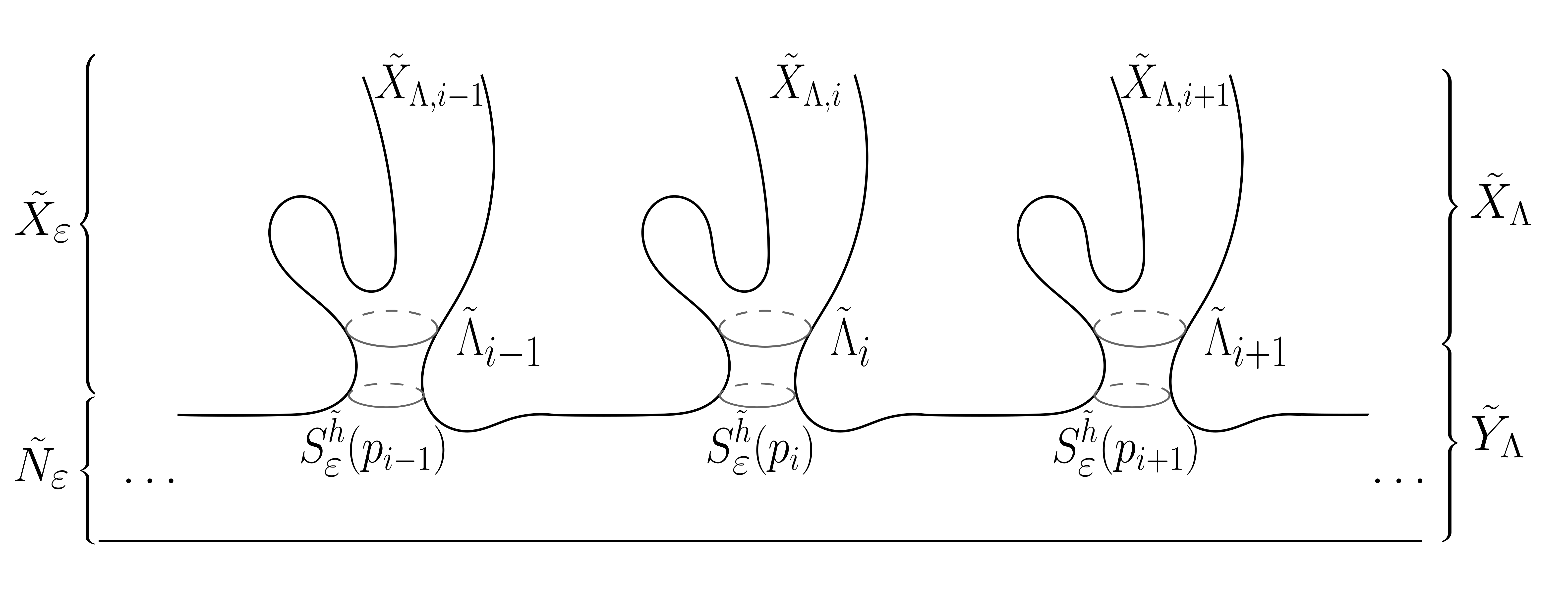
Figure 2. The covering space $\tilde{Y}=\tilde{N}\#_{\pi_{1}(N)}X$

2.2. Line construction

In this subsection we show that we can find a proper line contained in $\tilde{N}_{\varepsilon}$. Recall

Lemma 2.1 (Lemma 6 of [5, first version]).

Suppose $N$ is a smooth closed aspherical $n$-dimensional manifold. Then $\pi_{1}(N)$ is an infinite group, and every nontrivial element of it has infinite order.

Proof.

We include the proof for completeness. Since $\tilde{N}$ is contractible we have that $H_{n}(\tilde{N})=0$. Any closed orientable connected $n$-manifold $M$ satisfies $H_{n}(M)=\mathbb{Z}$, so $\tilde{N}$ is non-compact. Thus, $\pi_{1}(N)$ is an infinite group.

Take any element $[\sigma]\in\pi_{1}(N)$. Suppose the contrary, that $[\sigma]$ has finite order $k$. Let $C$ be the cyclic group generated by $[\sigma]$. Then the manifold $\tilde{N}/C$ is an Eilenberg–MacLane space $K(\mathbb{Z}_{k},1)$, which is homotopy equivalent to $S^{\infty}/\mathbb{Z}_{k}$. This is impossible, as $H_{l}(\tilde{N}/C)=0$ for all $l>n$. ∎

Fix a nontrivial element $[\sigma]\in\pi_{1}(N)$ and let $C$ be the subgroup generated by $[\sigma]$. Let $\overline{N}=\tilde{N}/C$ and let $\overline{\pi}:\overline{N}\to N$ be the covering map. Then $\overline{N}$ is an Eilenberg-MacLane space $K(\mathbb{Z},1)$, which is homotopy equivalent to $\mathbb{S}^{1}$. In particular, $H_{n}(\overline{N})=0$, and hence $\overline{N}$ is non-compact. Fix a simple closed non-contractible loop $\overline{\sigma}\subset\overline{N}$ such that $\overline{\sigma}$ is a generator of $\pi_{1}(\overline{N})\cong\mathbb{Z}$ and $\overline{\pi}(\overline{\sigma})\cap B^{h}_{\varepsilon}(p)=\emptyset$. Let $\tilde{\sigma}:\mathbb{R}\to\tilde{N}$ be the lift of $\overline{\sigma}$ in $\tilde{N}$. By our construction, $\tilde{\sigma}(\mathbb{R})\subset\tilde{N}_{\varepsilon}$, so this also induces a line in $\tilde{Y}$, which we also denote by $\tilde{\sigma}$.

Lemma 2.2.

There exists a constant $A$ such that

• $\tilde{\sigma}(\mathbb{R})\subset\tilde{N}_{\varepsilon}$;

• $\operatorname{dist}_{\tilde{g}}(\tilde{\sigma}(t_{1}),\tilde{\sigma}(t_{2}))\leq A|t_{1}-t_{2}|$ for all $t_{1},t_{2}\in\mathbb{R}$;

• $\lim_{|t_{1}-t_{2}|\to+\infty}\operatorname{dist}_{\tilde{g}}(\tilde{\sigma}(t_{1}),\tilde{\sigma}(t_{2}))=+\infty$,

where $\tilde{g}$ be the lifted metric of $g$ on $\tilde{Y}$.

Proof.

(i) follows from the construction of $\tilde{\sigma}$. Let $\overline{\sigma}:[0,1]\rightarrow N$ be a parametrization and set $A=\sup_{t\in[0,1]}|\overline{\sigma}^{\prime}(t)|_{g}$. Since $\tilde{\sigma}$ is the lift of $\overline{\sigma}$, then $\sup_{t\in\mathbb{R}}|\tilde{\sigma}^{\prime}(t)|_{\tilde{g}}=A$. For any $t_{1},t_{2}\in\mathbb{R}$ (we assume without loss of generality that $t_{1}\leq t_{2}$),

$$\operatorname{dist}_{\tilde{g}}(\tilde{\sigma}(t_{1}),\tilde{\sigma}(t_{2}))\leq\mathrm{length}_{\tilde{g}}(\tilde{\sigma}|_{[t_{1},t_{2}]})\leq A|t_{1}-t_{2}|,$$

which is (ii). For (iii), by applying the deck transformation, it suffices to show that

$$\lim_{t\to+\infty}\operatorname{dist}_{\tilde{g}}(\tilde{\sigma}(0),\tilde{\sigma}(t))=+\infty.$$

We argue by contradiction. Suppose that $\{t_{i}\}$ is a sequence such that

$$\lim_{i\rightarrow\infty}t_{i}=+\infty,\quad\operatorname{dist}_{\tilde{g}}(\tilde{\sigma}(0),\tilde{\sigma}(t_{i}))\leq C$$

for some constant $C$ independent of $i$. Let $[\cdot]$ be the greatest integer function. Then by (ii), we see that

$$\begin{split}\operatorname{dist}_{\tilde{g}}(\tilde{\sigma}(0),\tilde{\sigma}([t_{i}]))\leq{}&\operatorname{dist}_{\tilde{g}}(\tilde{\sigma}(0),\tilde{\sigma}(t_{i}))+\operatorname{dist}_{\tilde{g}}(\tilde{\sigma}(t_{i}),\tilde{\sigma}([t_{i}]))\\ \leq{}&C+A|t_{i}-[t_{i}]|\leq C+A.\end{split}$$

This implies that $\{\tilde{\sigma}([t_{i}])\}$ has a convergent subsequence. However, since $\tilde{\sigma}$ is the lift of $\overline{\sigma}$ and $\tilde{\sigma}([t_{i}])\in\pi^{-1}(\overline{\sigma}(0))$, $\{\tilde{\sigma}([t_{i}])\}$ does not admit any convergent subsequence, and we get a contradiction. ∎

2.3. Auxiliary short function

In this Subsection we construct some auxiliary functions for later use. Since their Lipschitz constant is strictly less than one, we refer to them as short functions.

Lemma 2.3.

Let $\Lambda$ be a smooth closed hypersurface $\Lambda\subset X_{\varepsilon}$. Then there is a proper smooth function

$$\rho_{\Lambda}:X_{\Lambda}\to[0,+\infty)$$

such that

• $\rho_{\Lambda}\equiv 0$ in an open neighborhood of $\Lambda$;

• $|\mathrm{d}\rho_{\Lambda}|_{g}<1$.

Proof.

Fix a small positive constant $\tau$ such that the distance function

$$\mathfrak{d}(\cdot):=\operatorname{dist}_{g}(\cdot,\Lambda)$$

is smooth in the $\tau$-neighborhood of $\Lambda$ in $Y$. We start with the function

$$\rho_{1}=\min\{0,\mathfrak{d}-\tau\}.$$

Through a very standard mollification as in [21, Appendix], we are able to construct a proper smooth function $\rho_{2}:X_{\Lambda}\to[0,+\infty)$ having bounded Lipschitz constant and satisfying $\rho_{2}\equiv 0$ in the $(\tau/2)$-neighborhood of $\Lambda$. After taking

$$\rho_{\Lambda}=\frac{\rho_{2}}{\operatorname{Lip}\rho_{2}+1}$$

we can guarantee $|\mathrm{d}\rho_{\Lambda}|_{g}<1$ and this completes the proof. ∎

From (2.1) we see that

$$\operatorname{dist}_{\tilde{g}}(\tilde{X}_{\Lambda_{1},i},\tilde{X}_{\Lambda_{1},j})\geq 6d_{\Lambda_{1}}\mbox{ when }i\neq j.$$

We construct suitable “lifts” of $\rho_{\Lambda_{1}}$ for later use.

Lemma 2.4.

For each $i$ we can construct a smooth function

$$\tilde{\rho}_{i}:\tilde{Y}\to\mathbb{R}$$

such that

• the set $\tilde{\rho}_{i}^{-1}([-d_{\Lambda_{1}},d_{\Lambda_{1}}])$ is contained in $\tilde{Y}_{\Lambda_{1}}$;

• Let $\rho_{\Lambda_{1}}$ be the function from Lemma 2.3. Then there is a constant $d_{\Lambda_{1}}^{\prime}>d_{\Lambda_{1}}$ such that

  $$\tilde{\rho}_{i}=-\rho_{\Lambda_{1}}\circ\pi-d_{\Lambda_{1}}^{\prime}\mbox{ in }\tilde{X}_{\Lambda_{1},i}$$

  and

  $$\tilde{\rho}_{i}=\rho_{\Lambda_{1}}\circ\pi+d_{\Lambda_{1}}^{\prime}\mbox{ in }\tilde{X}_{\Lambda_{1},j}\mbox{ when }j\neq i;$$

• $|\mathrm{d}\tilde{\rho}_{i}|_{\tilde{g}}<1$.

Proof.

Let $\mathfrak{d}$ be the signed distance function to $\tilde{\Lambda}_{1,i}$ taking negative values in $\tilde{X}_{\Lambda_{1},i}$. Put $\hat{\rho}_{1}=\mathfrak{d}-3d_{\Lambda_{1}}$. Through a standard mollification as in [1] or [21, Appendix] for any $\tau>0$ we can find a smooth proper function $\hat{\rho}$ satisfying $|\hat{\rho}-\hat{\rho}_{1}|\leq\tau\mbox{ and }|\mathrm{d}\hat{\rho}|_{\tilde{g}}\leq 1+\tau.$ Define

$$\hat{\rho}_{2}=\frac{\hat{\rho}}{1+2\tau}.$$

By taking $\tau$ small enough we can guarantee

$$\hat{\rho}_{2}\leq-2d_{\Lambda_{1}}\mbox{ in }\tilde{X}_{\Lambda_{1},i}$$

and

$$\hat{\rho}_{2}\geq 2d_{\Lambda_{1}}\mbox{ in }\tilde{X}_{\Lambda_{1},j}\mbox{ when }j\neq i.$$

Take a smooth and even cut-off function $\eta:(-\infty,+\infty)\to[0,1]$ such that $\eta\equiv 1$ in $[-d_{\Lambda_{1}},d_{\Lambda_{1}}]$ and $\eta\equiv 0$ in $(-\infty,-\frac{3}{2}d_{\Lambda_{1}}]\cup[\frac{3}{2}d_{\Lambda_{1}},+\infty)$. Denote

$$\hat{\rho}_{3}=\int_{0}^{\hat{\rho}_{2}}\eta(t)\,\mathrm{d}t$$

and

$$d_{\Lambda_{1}}^{\prime}=\int_{0}^{2d_{\Lambda_{1}}}\eta(t)\,\mathrm{d}t.$$

Define

$$\tilde{\rho}_{i}=\left\{\begin{array}[]{cc}\hat{\rho}_{3}&\mbox{ in }\tilde{Y}_{\Lambda_{1}};\\[2.84526pt] -\rho_{\Lambda_{1}}\circ\pi-d_{\Lambda_{1}}^{\prime}&\mbox{ in }\tilde{X}_{\Lambda_{1},i};\\[2.84526pt] \rho_{\Lambda_{1}}\circ\pi+d_{\Lambda_{1}}^{\prime}&\mbox{ in }\cup_{j\neq i}\tilde{X}_{\Lambda_{1},j}.\end{array}\right.$$

Then it is easy to verify that $\tilde{\rho}_{i}$ satisfies all the desired properties. ∎

2.4. Weight functions

Lemma 2.5.

Given any positive constants $\nu_{0}$ and $d_{0}$, there is a positive constant $\delta_{0}=\delta_{0}(\nu_{0},d_{0})$ such that for any positive constant $\delta\in(0,\delta_{0})$ we can find $T_{\delta}>d_{0}$ and a smooth function

$$h_{\delta}:(-T_{\delta},T_{\delta})\to\mathbb{R}$$

such that

• $\lim_{t\to\pm T_{\delta}}h_{\delta}(t)=\mp\infty$ and $h_{\delta}^{\prime}<0$;

• $h_{\delta}^{2}-2|\mathrm{d}h_{\delta}|+\nu_{0}\chi_{[-d_{0},d_{0}]}\geq\delta$.

Proof.

Take a smooth cut-off function $\eta:(-\infty,+\infty)\to[0,1]$ such that $\eta\equiv 1$ in $(-\infty,-d_{0}]$, $\eta\equiv 0$ in $[d_{0},+\infty)$ and $\eta^{\prime}\leq 0$. Take $\delta_{0}$ to be a positive constant no greater than $\nu_{0}/2$ such that

$$\delta_{0}\|2\eta-1\|_{C^{0}}^{2}+2\sqrt{\delta_{0}}\|2\eta-1\|_{C^{1}}<\nu_{0}/2.$$ (2.2)

For any $\delta\in(0,\delta_{0})$ and integer $k>d_{0}$ we denote

$$f_{k}^{+}:(-k,+\infty)\to(\sqrt{\delta},+\infty),\,t\mapsto\sqrt{\delta}\coth\left(\frac{\sqrt{\delta}}{2}(k+t)\right),$$

and

$$f_{k}^{-}:(-\infty,k)\to(-\infty,-\sqrt{\delta}),\,t\mapsto-\sqrt{\delta}\coth\left(\frac{\sqrt{\delta}}{2}(k-t)\right).$$ (2.3)

It is easy to verify $(f_{k}^{\pm})^{2}+2(f_{k}^{\pm})^{\prime}=\delta$, $(f_{k}^{\pm})^{\prime}<0$ and $f_{k}^{+}>f_{k}^{-}$. Define

$$h_{\delta}=\eta f_{k}^{+}+(1-\eta)f_{k}^{-}:(-k,k)\to\mathbb{R}$$

with $k$ to be determined later. Then it is easy to verify

$$\lim_{t\to\pm k}h_{\delta}=\lim_{t\to\pm k}f_{k}^{\mp}=\mp\infty$$

and

$$h_{\delta}^{\prime}=\eta(f^{+}_{k})^{\prime}+(1-\eta)(f_{k}^{-})^{\prime}+\eta^{\prime}(f^{+}_{k}-f_{k}^{-})<0.$$

Notice that $h_{\delta}$ converges smoothly to the function $(2\eta-1)\sqrt{\delta}$ in the closed interval $[-d_{0},d_{0}]$ as $k\to\infty$. From estimate (2.2) we can take $k$ large enough such that

$$h_{\delta}^{2}-2|\mathrm{d}h_{\delta}|+\nu_{0}>\nu_{0}/2\geq\delta\mbox{ in }[-d_{0},d_{0}].$$

Outside $[-d_{0},d_{0}]$ we have $h_{\delta}^{2}-2|\mathrm{d}h_{\delta}|=\delta$ and so $h_{\delta}$ satisfies all the desired properties. ∎

Lemma 2.6.

Given any positive constants $\nu_{0}$ and $d_{0}$, there is a positive constant $\delta_{0}=\delta_{0}(\nu_{0},d_{0})$ such that for any positive constant $\delta\in(0,\delta_{0})$, we can find $T_{\delta}>d_{0}$ and a smooth function

$$h_{\delta}:[0,T_{\delta})\to(-\infty,0]$$

such that

• $h_{\delta}\equiv 0$ around $t=0$, $\lim_{t\to T_{\delta}}h_{\delta}(t)=-\infty$ and $h_{\delta}^{\prime}\leq 0$;

• $h_{\delta}^{2}-2|\mathrm{d}h_{\delta}|+\nu_{0}\chi_{[0,d_{0}]}\geq\delta$.

Proof.

The proof is similar to that of Lemma 2.5. Take a smooth cut-off function $\eta:[0,+\infty)\to[0,1]$ such that $\eta\equiv 1$ around $t=0$, $\eta\equiv 0$ in $[d_{0},+\infty)$ and $\eta^{\prime}\leq 0$. Take $\delta_{0}$ to be a positive constant no greater than $\nu_{0}/2$ such that

$$\delta_{0}\|\eta-1\|_{C^{0}}^{2}+2\sqrt{\delta_{0}}\|\eta-1\|_{C^{1}}<\nu_{0}/2.$$

For any $\delta\in(0,\delta_{0})$ and integer $k>d_{0}$ we take $h_{\delta}=(1-\eta)f_{k}^{-},$ where $f_{k}^{-}$ is the function from (2.3). As $k\to+\infty$ the function $h_{\delta}$ converges smoothly to $-\sqrt{\delta}(1-\eta)$ and so by taking $k$ large enough we can guarantee

$$h_{\delta}^{2}-2|\mathrm{d}h_{\delta}|+\nu_{0}\geq\nu_{0}/2\geq\delta\mbox{ when }t\in[0,d_{0}].$$

Outside $[-d_{0},d_{0}]$ we have $h_{\delta}^{2}-2|\mathrm{d}h_{\delta}|=\delta$ from the definition of $f_{k}^{-}$. The remaining properties can be verified easily and we complete the proof. ∎

2.5. Topology

Here we collect some topological facts about $\tilde{Y}$. To deal with the arbitrary ends $\tilde{X}_{\varepsilon}$ over which we have no control, we use relative homology theory so that the ends $\tilde{X}_{\varepsilon}$ have no impact on our topological analysis. All the homology groups in this paper are assumed to have $\mathbb{Z}$ coefficients, unless otherwise noted.

Lemma 2.7.

We have

$$H_{k}(\tilde{Y},\tilde{X}_{\varepsilon})=0$$

for all integers $k\geq 2$. Moreover, if $\gamma$ is a closed curve in $\tilde{Y}$, then $[\gamma]=0\in H_{1}(\tilde{Y},\tilde{X}_{\varepsilon})$.

Proof.

From excision we have

$$H_{k}(\tilde{Y},\tilde{X}_{\varepsilon})=H_{k}\left(\tilde{N}_{\varepsilon},\bigcup_{i}\partial B^{\tilde{h}}_{\varepsilon}(p_{i})\right)=H_{k}\left(\tilde{N},\bigcup_{i}B_{\varepsilon}^{\tilde{h}}(p_{i})\right).$$

From the exact sequence of pair we have

$$H_{k}\left(\bigcup_{i}B_{\varepsilon}^{\tilde{h}}(p_{i})\right)\to H_{k}(\tilde{N})\to H_{k}\left(\tilde{N},\bigcup_{i}B_{\varepsilon}^{\tilde{h}}(p_{i})\right)\to H_{k-1}\left(\bigcup_{i}B_{\varepsilon}^{\tilde{h}}(p_{i})\right).$$

Notice that the first and fourth terms are zero when $k\geq 2$ and so it follows from the contractibility of $\tilde{N}$ that

$$H_{k}\left(\tilde{N},\bigcup_{i}B^{\tilde{h}}_{\varepsilon}(p_{i})\right)=H_{k}(\tilde{N})=0.$$

Since $\tilde{Y}=\tilde{N}\#_{\pi_{1}(N)}X$, we can fix a continuous map

$$F:\tilde{Y}\to\tilde{N}\mbox{ with }F|_{\tilde{N}_{\varepsilon}}=\mathrm{id}:\tilde{N}_{\varepsilon}\to\tilde{N}_{\varepsilon}.$$

From excision property we see that $F_{*}:H_{1}(\tilde{Y},\tilde{X}_{\varepsilon})\to H_{1}(\tilde{N},\bigcup_{i}B_{\varepsilon}^{\tilde{h}}(p_{i}))$ is an isomorphism. To see $[\gamma]=0\in H_{1}(\tilde{Y},\tilde{X}_{\varepsilon})$ for any closed curve $\gamma$, we just need to show $[F\circ\gamma]=0\in H_{1}(\tilde{N},\bigcup_{i}B_{\varepsilon}^{\tilde{h}}(p_{i}))$. It is well-known that the curve $F\circ\gamma$ can be deformed continuously to a new closed curve which avoids touching all balls $B_{\varepsilon}^{\tilde{h}}(p_{i})$. This yields $\partial[F\circ\gamma]=0$ under the map

$$\partial:H_{1}\left(\tilde{N},\bigcup_{i}B_{\varepsilon}^{\tilde{h}}(p_{i})\right)\to H_{0}\left(\bigcup_{i}B_{\varepsilon}^{\tilde{h}}(p_{i})\right).$$

The exactness then implies that $[F\circ\gamma]$ must lie in the image of

$$H_{1}(\tilde{N})\to H_{1}\left(\tilde{N},\bigcup_{i}B_{\varepsilon}^{\tilde{h}}(p_{i})\right).$$

Therefore we obtain $[F\circ\gamma]=0$ from the fact that $\tilde{N}$ is contractible (and in particular $H_{1}(\tilde{N})=0$), which completes the proof. ∎

Moreover, we have the following quantitative filling lemma, which is a relative version of [5, Proposition 10].

Lemma 2.8.

For any $k\in\mathbb{N}_{+}$ there is a function $F:(0,+\infty)\to(0,+\infty)$ depending only on the triple $(Y,N_{\varepsilon},g)$ such that if $C$ is a relative $k$-boundary in $\mathcal{B}_{k}(\tilde{Y},\tilde{X}_{\varepsilon})$ contained in some geodesic ball $B_{r}^{\tilde{g}}(\tilde{q})$ of $(\tilde{Y},\tilde{g})$ with $\tilde{q}\in\tilde{N}_{\varepsilon}$, then we can find a relative $(k+1)$-chain $\Gamma\in\mathcal{Z}_{k+1}(\tilde{Y},\tilde{X}_{\varepsilon})$ contained in the geodesic ball $B_{F(r)}^{\tilde{g}}(\tilde{q})$ of $(\tilde{Y},\tilde{g})$ with $\partial\Gamma=C$ modulo $\tilde{X}_{\varepsilon}$.

Proof.

Fix a point $q_{0}\in\tilde{N}_{\varepsilon}\subset\tilde{Y}$. For any $r>0$ the kernel of the inclusion

$$i_{*}:H_{k}(B_{r}^{\tilde{g}}(q_{0}),\tilde{X}_{\varepsilon})\to H_{k}(\tilde{Y},\tilde{X}_{\varepsilon})$$

is finitely generated and so there exists some $R_{0}=R_{0}(r)<+\infty$ such that each relative $k$-boundary in $\mathcal{B}_{k}(\tilde{Y},\tilde{X}_{\varepsilon})$ contained in ball $B_{r}^{\tilde{g}}(q_{0})$ can be filled in $B_{R_{0}}^{\tilde{g}}(q_{0})$.

For any point $q\in\tilde{N}_{\varepsilon}\subset\tilde{Y}$ other than $q_{0}$, there is a deck transformation $\Psi$ so that $d(q_{0},\Psi(q))\leq D_{0}:=\operatorname{diam}(N_{\varepsilon},g)$. As such, we have $\Psi(B_{r}^{\tilde{g}}(q))\subset B_{r+D_{0}}^{\tilde{g}}(q_{0})$. Now let $C$ be a relative $k$-boundary in $\mathcal{B}_{k}(\tilde{Y},\tilde{X}_{\varepsilon})$ contained in $B_{r}^{\tilde{g}}(q)$, then $\Psi_{\#}C$ is a relative $k$-boundary contained in $B_{r+D_{0}}^{\tilde{g}}(q_{0})$. From previous discussion we can find a relative $(k+1)$-chain $\Gamma\in\mathcal{Z}_{k+1}(\tilde{Y},\tilde{X}_{\varepsilon})$ contained in $B_{R_{0}(r+D_{0})}^{\tilde{g}}(q_{0})$ such that $\partial\Gamma=\Psi_{\#}C$ modulo $\tilde{X}_{\varepsilon}$. Then it follows that $(\Psi^{-1})_{\#}\Gamma$ is a relative $(k+1)$-chain with relative $k$-boundary $\Gamma$ which is contained in $B_{R_{0}(r+D_{0})+D_{0}}^{\tilde{g}}(q)$. The proof is completed by taking $F(r)=R_{0}(r+D_{0})+D_{0}$. ∎

2.6. $\mathbb{T}^{l}$-invariant variational problems

The results here are similar to the ones in [5, Sections 3-4] about warped $\mu$-bubbles and free boundary warped $\mu$-bubbles, but we present them using a warped product formulation.

Definition 2.9.

Let $(M,g)$ be a Riemannian manifold possibly with non-empty boundary and $\Gamma$ be a smooth portion of $\partial M$. Let $R$ and $H$ be smooth functions on $M$ and $\Gamma$ respectively. We say that $(M,\Gamma)$ has $\mathbb{T}^{l}$-stablized scalar-mean curvature $(R,H)$ if there are $l$ positive smooth functions $v_{1},v_{2},\ldots,v_{l}$ on $M$ such that $(M\times\mathbb{T}^{l},g+\sum_{i}v_{i}^{2}\mathrm{d}\theta_{i}^{2})$ has scalar curvature $\tilde{R}$ in $\hat{M}:=M\times\mathbb{T}^{l}$ and has mean curvature $\tilde{H}$ on $\Gamma\times\mathbb{T}^{l}$, where $\tilde{R}$ and $\tilde{H}$ are $\mathbb{T}^{l}$-invariant extension of $R$ and $H$ respectively. (Of course $\operatorname{dim}M+l\geq 2$ is required to compute the scalar curvature.)

Lemma 2.10.

Let $2\leq n\leq 7$. Let $(M^{n},g)$ be a complete Riemannian manifold and $S$ be an embedded submanifold in $M$ with codimension two and $0=[S]\in H_{n-2}(M)$. If $M$ has $\mathbb{T}^{l}$-stablized scalar curvature $R$, then we can construct a properly embedded, complete hypersurface $\Sigma$ with $\partial\Sigma=S$ and $\mathring{\Sigma}$ has $\mathbb{T}^{l+1}$-stablized scalar curvature $R^{\prime}$ which is no less than $R|_{\Sigma}$.

Proof.

Denote $\hat{M}=M\times\mathbb{T}^{l}$. Since $M$ has $\mathbb{T}^{l}$-stablized scalar curvature $R$, there are finitely many smooth positive functions $v_{1},v_{2},\ldots,v_{l}$ on $M$ such that the warped product metric

$$\hat{g}=g+\sum_{i=1}^{l}v_{i}^{2}\mathrm{d}\theta_{i}^{2}$$ (2.4)

satisfies $R(\hat{g})=\tilde{R}$, where $\tilde{R}$ is the $\mathbb{T}^{l}$-invariant extension of $R$ on $\hat{M}$. We would like to minimize the area functional among hypersurfaces in the form of $\Sigma\times\mathbb{T}^{l}$ with $\partial\Sigma=S$. This is equivalent to solving the Plateau problem for $S$ in the Riemannian manifold $(M,\tilde{g})$ with

$$\tilde{g}=\left(\prod_{i}v_{i}\right)^{\frac{2}{n-1}}g.$$ (2.5)

It follows from a modification of the proof of [30, Lemma 34.1] and the regularity theory for mass-minimizing current that when $2\leq n\leq 7$ we can find a properly embedded (possibly non-compact) hypersurface $\Sigma$ minimizing the area functional with $\partial\Sigma=S$.

Next we show that $\mathring{\Sigma}$ has $\mathbb{T}^{l+1}$-stablized scalar curvature $R^{\prime}$ which is no less than $R$. Notice that $\Sigma\times\mathbb{T}^{l}$ is actually a constrained area minimizer in $(\hat{M},\hat{g})$ among $\mathbb{T}^{l}$-invariant hypersurfaces. From the $\mathbb{T}^{l}$-invariance of $(\hat{M},\hat{g})$ we see that the mean curvature of $\Sigma\times\mathbb{T}^{l}$ is $\mathbb{T}^{l}$-invariant. This yields that $\Sigma\times\mathbb{T}^{l}$ has to be a minimal hypersurface as a constrained area-minimizer. We claim that $\Sigma\times\mathbb{T}^{l}$ is also stable. To see this we consider a $\mathbb{T}^{l}$-invariant exhaustion $U_{i}\times\mathbb{T}^{l}$ of $\Sigma\times\mathbb{T}^{l}$. The key is to notice that the Jacobi operator

$$\mathcal{J}=-\Delta-(\mathrm{Ric}(\nu)+|A|^{2})$$

(corresponding to the second variation of the area functional $\mathcal{H}^{n+l}_{\hat{g}}(\cdot)$) on $\Sigma\times\mathbb{T}^{l}$ is also $\mathbb{T}^{l}$-invariant. The uniqueness of the first eigenfunction (up to a scale) implies that the first eigenfunction with Dirichlet boundary condition of the Jacobi operator on $U_{i}\times\mathbb{T}^{l}$ is again $\mathbb{T}^{l}$-invariant. The property of constrained area minimizer then yields the stability of $\Sigma\times\mathbb{T}^{l}$. Notice that the properness of $\Sigma$ actually implies the completeness of $\Sigma\times\mathbb{T}^{l}$.

Now the argument can be divided into two cases.

Case 1. $\Sigma$ is compact. We take $\tilde{v}_{l+1}$ to be the first eigenfunction with the Dirichlet boundary condition of the Jacobi operator. Then $\tilde{v}_{l+1}$ is $\mathbb{T}^{l}$-invariant from previous discussion and it induces a smooth function $v_{l+1}$ on $\Sigma$ with $v_{l+1}>0$ in $\mathring{\Sigma}$. And we have $\mathcal{J}\tilde{v}_{l+1}\geq 0$.

Case 2. $\Sigma$ is non-compact. Repeating Fischer-Colbrie–Schoen’s construction [7] we can construct a $\mathbb{T}^{l}$-invariant function $\tilde{v}_{l+1}$ on $\Sigma\times\mathbb{T}^{l}$ such that $\mathcal{J}\tilde{v}_{l+1}=0$ and $\tilde{v}_{l+1}>0$ in $\mathring{\Sigma}\times\mathbb{T}^{l}$. Again it induces a smooth function $v_{l+1}$ on $\Sigma$ with $v_{l+1}>0$ in $\mathring{\Sigma}$.

In both cases, applying Schoen–Yau’s rearrangement trick and Fischer-Colbrie–Schoen’s warping construction we can compute

$$R(\hat{g}^{\prime})=R(\hat{g}|_{\Sigma\times\mathbb{T}^{l}})-\frac{2\Delta\tilde{v}_{l+1}}{\tilde{v}_{l+1}}\geq R(\hat{g})|_{\Sigma\times\mathbb{T}^{l}}=\tilde{R}\,\mbox{ in }\mathring{\Sigma}\times\mathbb{T}^{l},$$

where

$$\hat{g}^{\prime}=g|_{\Sigma}+\sum_{i=1}^{l}(v_{i}|_{\Sigma})^{2}\mathrm{d}\theta_{i}^{2}+v_{l+1}^{2}\mathrm{d}\theta_{l+1}^{2}.$$ (2.6)

That is, $\mathring{\Sigma}$ has $\mathbb{T}^{l+1}$-stablized scalar curvature $R^{\prime}$ which is no less than $R|_{\Sigma}$. ∎

Lemma 2.11.

Let $2\leq n\leq 7$. Let $(M^{n},g)$ be a closed Riemannian manifold and $\beta$ be an $(n-1)$-homology class with $\beta\neq 0\in H_{n-1}(M)$. If $M$ has $\mathbb{T}^{l}$-stablized scalar curvature $R$, then we can construct an embedded hypersurface $\Sigma$ with integer multiplicity such that $\Sigma$ has $\mathbb{T}^{l+1}$-stablized scalar curvature $R^{\prime}$ which is no less than $R|_{\Sigma}$ and the metric completion of $M-\Sigma$ associated with its boundary has $\mathbb{T}^{l}$-stablized scalar-mean curvature $(R,0)$.

Proof.

Since $M$ has $\mathbb{T}^{l}$-stablized scalar curvature $R$, there are finitely many smooth positive functions $v_{1},v_{2},\ldots,v_{l}$ on $M$ such that the warped product metric $\hat{g}$ defined by (2.4) satisfies $R(\hat{g})=\tilde{R}$, where $\tilde{R}$ is the $\mathbb{T}^{l}$-invariant extension of $R$ on $\hat{M}$. It follows from geometric measure theory that we can find an embedded hypersurface $\Sigma$ with integer multiplicity representing the homology class $\beta$ which is homologically area-minimizing in $(M,\tilde{g})$, where $\tilde{g}$ is the metric defined by (2.5). From a similar argument as in the proof of Lemma 2.10 we conclude that $\Sigma$ has $\mathbb{T}^{l+1}$-stablized scalar curvature $R^{\prime}$ which is no less than $R|_{\Sigma}$. The last assertion comes immediately from the construction of $\Sigma$. ∎

Definition 2.12.

We say that $(M,\partial_{\pm},g)$ is a Riemannian band if $(M,g)$ is a compact Riemannian manifold with boundary and $\partial_{+}$ and $\partial_{-}$ are two disjoint non-empty smooth compact portions of $\partial M$ such that $\overline{\partial M-(\partial_{+}\cup\partial_{-})}$ is also a compact smooth portion of $\partial M$.

Lemma 2.13.

Let $2\leq n\leq 7$. Let $(M,\partial_{\pm},g)$ be a Riemannian band with $\overline{\partial M-(\partial_{+}\cup\partial_{-})}=\emptyset$ and $\operatorname{dist}(\partial_{+},\partial_{-})>2d_{0}$. If M has $\mathbb{T}^{l}$-stablized scalar curvature $R$, then we can find an embedded hypersurface $\Sigma$ bounding a region with $\partial_{-}$ which has $\mathbb{T}^{l+1}$-stablized scalar curvature $R^{\prime}$ with

$$R^{\prime}\geq R|_{\Sigma}-\frac{\pi^{2}}{d_{0}^{2}}.$$

Proof.

Since $\operatorname{dist}(\partial_{+},\partial_{-})>2d_{0}$, we can construct a smooth short function $\rho:(M,\partial_{\pm})\to([-d_{0},d_{0}],\pm d_{0})$ such that $\rho^{-1}(d_{0})=\partial_{+}$, $\rho^{-1}(-d_{0})=\partial_{-}$ and $\operatorname{Lip}\rho<1$. Take

$$h=-\frac{n+l-1}{n+l}\frac{\pi}{d_{0}}\tan\left(\frac{\pi}{2d_{0}}t\right)$$

and $h$ satisfies

$$\frac{n+l}{n+l-1}h^{2}-2|\mathrm{d}h|=-\frac{n+l-1}{n+l}\frac{\pi^{2}}{d_{0}^{2}}.$$

Since $M$ has $\mathbb{T}^{l}$-stablized scalar curvature $R$, there are finitely many smooth positive functions $v_{1},v_{2},\ldots,v_{l}$ on $M$ such that the warped product metric $\hat{g}$ defined by (2.4) satisfies $R(\hat{g})=\tilde{R}$, where $\tilde{R}$ is the $\mathbb{T}^{l}$-invariant extension of $R$ on $\hat{M}=M\times\mathbb{T}^{l}$. Let us consider the following minimization problem. Set

$$\mathcal{A}^{h}(\Omega)=\mathcal{H}^{n-1}_{\tilde{g}}(\partial\Omega\cap\mathring{M})-\int_{\mathring{M}}(\chi_{\Omega}-\chi_{\Omega_{0}})(h\circ\rho)\left(\prod_{i}v_{i}\right)^{\frac{1}{n-1}}\,\mathrm{d}\mathcal{H}^{n}_{\tilde{g}},$$

where $\tilde{g}$ is the metric defined by (2.5), $\Omega_{0}=\rho^{-1}((-\infty,0])$ and $\Omega$ belongs to the class

$$\mathcal{C}=\{\text{Caccioppoli sets $\Omega$ in $M$ such that $\Omega\Delta\Omega_{0}\Subset\mathring{M}$}\}.$$ (2.7)

Notice that the function

$$\tilde{h}:=(h\circ\rho)\left(\prod_{i}v_{i}\right)^{\frac{1}{n-1}}$$ (2.8)

takes value $+\infty$ on $\partial_{-}$ and takes value $-\infty$ on $\partial_{+}$. It follows from [34, Proposition 2.1] that we can find a smooth minimizer $\Omega_{\mathrm{min}}$ of $\mathcal{A}^{h}$ in $\mathcal{C}$.

Let $\Sigma=\partial\Omega_{\mathrm{min}}\cap\mathring{M}$. Then $\Sigma$ and $\partial_{-}$ bound the region $\Omega_{\mathrm{min}}$. With a similar argument as in the proof of Lemma 2.10 by taking $v_{l+1}$ to be the first eigenfunction of the Jacobi operator (associated to the functional $\mathcal{A}^{h}$) we obtain

$$R(\hat{g}^{\prime})\geq R(\hat{g})|_{\Sigma\times\mathbb{T}^{l}}+\left(\frac{n+l}{n+l-1}h^{2}-2|\mathrm{d}h|\right)\circ\rho\geq R(\hat{g})|_{\Sigma\times\mathbb{T}^{l}}-\frac{\pi^{2}}{d_{0}^{2}},$$

where $\hat{g}^{\prime}$ is defined by (2.6). ∎

Lemma 2.14.

Let $2\leq n\leq 7$. Let $(M,\partial_{\pm},g)$ be a Riemannian band with $\Gamma:=\overline{\partial M-(\partial_{+}\cup\partial_{-})}\neq\emptyset$ and $\operatorname{dist}(\partial_{+},\partial_{-})>2d_{0}$. If the dihedral angles between $\Gamma$ and $\partial_{+}\cup\partial_{-}$ are less than $\pi/2$ and $(M,\Gamma)$ has $\mathbb{T}^{l}$-stablized scalar-mean curvature $(R,H)$, then we can find a hypersurface $\Sigma$ possibly with boundary $\partial\Sigma$ intersecting $\Gamma$ orthogonally such that

• $\Sigma$ and $\partial_{-}$ bound a relative region $\Omega$ relative to $\Gamma$, namely we have $\partial\Omega-(\Sigma\cup\partial_{-})\subset\Gamma$;

• $(\Sigma,\partial\Sigma)$ has $\mathbb{T}^{l+1}$-stablized scalar-mean curvature $(R^{\prime},H^{\prime})$ where $R^{\prime}\geq R-\pi^{2}/d_{0}^{2}$ and $H^{\prime}=H$.

Proof.

The proof is almost the same as that of Lemma 2.13 except that the solution to the minimizing problem for the functional $\mathcal{A}^{h}$ from [34, Proposition 2.1] needs some modification due to existence of the corner $(\partial_{+}\cup\partial_{-})\cap\Gamma$. The key to finding a smooth minimizer of $\mathcal{A}^{h}$ is the existence of a minimizing sequence $\Omega_{i}$ whose reduced boundary $\partial\Omega_{i}\cap\mathring{M}$ stays away from a fixed neighborhood of $\partial_{+}\cup\partial_{-}$. We will only provide some details on this point since the rest of the argument is rather standard.

Let $\Omega_{i}$ be a minimizing sequence of the functional $\mathcal{A}^{h}$ in $\mathcal{C}$. Namely, we have

$$\lim_{i\to\infty}\mathcal{A}^{h}(\Omega_{i})=\inf_{\Omega\in\mathcal{C}}\mathcal{A}^{h}(\Omega).$$

We show how to modify $\Omega_{i}$ to obtain a new minimizing sequence $\tilde{\Omega}_{i}$ such that the reduced boundary $\partial\tilde{\Omega}_{i}\cap\mathring{M}$ stays away from a fixed neighborhood of $\partial_{+}$. The modification can be done similarly around $\partial_{-}$ and this provides the desired minimizing sequence. From continuity we can find a family of tubular neighborhoods $\{\mathcal{N}_{s}\}_{s\in(0,s_{0}]}$ of $\partial_{+}$ such that

• $\cap_{s}\mathcal{N}_{s}=\partial_{+}$;

• $\partial\mathcal{N}_{s}\cap\mathring{M}$ are equidistant hypersurfaces to $\partial_{+}$ which intersect $\Gamma$ in acute angles (the inner product of outward unit normals of $\partial\mathcal{N}_{s}\subset\mathcal{N}_{s}$ and $\Gamma\subset M$ is positive);

• $\partial\mathcal{N}_{s}$ has mean curvature $H_{s}$ with respect to outward unit normal of $\partial\mathcal{N}_{s}\subset\mathcal{N}_{s}$, where $H_{s}<-\tilde{h}|_{\partial\mathcal{N}_{s}}$ and $\tilde{h}$ is the function defined by (2.8).

Define

$$\tilde{\Omega}_{i}=\Omega_{i}-\mathcal{N}_{s_{0}}.$$

Clearly $\tilde{\Omega}_{i}$ still belongs to the class $\mathcal{C}$ as defined in (2.7). It remains to show $\mathcal{A}^{h}(\tilde{\Omega}_{i})\leq\mathcal{A}^{h}(\Omega_{i})$. By the definition of $\mathcal{A}^{h}$ we can compute

$$\begin{split}\mathcal{A}^{h}(\tilde{\Omega}_{i})-&\mathcal{A}^{h}(\Omega_{i})=\int_{\Omega_{i}\cap\tilde{N}_{s_{0}}}\tilde{h}\,\mathrm{d}\mathcal{H}^{n}_{\tilde{g}}\\ &+\mathcal{H}^{n-1}_{\tilde{g}}(\partial\mathcal{N}_{s_{0}}\cap\Omega_{i}\cap\mathring{M})-\mathcal{H}^{n-1}_{\tilde{g}}(\partial\Omega_{i}\cap\tilde{N}_{s_{0}}\cap\mathring{M}).\end{split}$$

Let $X$ be the unit outward normal vector field determined by $\partial\mathcal{N}_{s}\subset\mathcal{N}_{s}$. Then the sum of the area terms in the second line is no greater than

$$\int_{\partial\mathcal{N}_{s_{0}}\cap\Omega_{i}\cap\mathring{M}}X\cdot X\,\mathrm{d}\mathcal{H}^{n-1}_{\tilde{g}}+\int_{\partial\Omega_{i}\cap\tilde{N}_{s_{0}}\cap\mathring{M}}X\cdot\nu\,\mathrm{d}\mathcal{H}^{n-1}_{\tilde{g}},$$

where $\nu$ is the unit outward normal of $\partial\Omega_{i}\subset\Omega_{i}$. It follows from the divergence theorem that the above terms equal to

$$\int_{\Omega_{i}\cap\mathcal{N}_{s}}\mathrm{div}\,X\,\mathrm{d}\mathcal{H}^{n}_{\tilde{g}}-\int_{\Omega_{i}\cap\mathcal{N}_{s}\cap\Gamma}X\cdot\mathbf{n}\,\mathrm{d}\mathcal{H}^{n-1}_{\tilde{g}},$$

where $\mathbf{n}$ is the outward unit normal of $\Gamma\subset M$. Combining with the acute-angle condition we finally obtain

$$\mathcal{A}^{h}(\tilde{\Omega}_{i})-\mathcal{A}^{h}(\Omega_{i})\leq\int_{\Omega_{i}\cap\mathcal{N}_{s_{0}}}(\tilde{h}+H_{s})\,\mathrm{d}\mathcal{H}^{n}_{\tilde{g}}\leq 0.$$

This completes the proof. ∎

2.7. Inradius estimate and intrinsic diameter estimate

Definition 2.15.

Let $(M,\partial M,g)$ be a Riemannian manifold with non-empty boundary and $\Gamma$ be a smooth (possibly empty) portion of $\partial M$ such that $\partial M\neq\Gamma$. The inradius of $(M,\partial M,\Gamma)$ is defined to be

$$r_{\mathrm{in}}(M,\partial M,\Gamma)=\sup_{p\in M}\operatorname{dist}_{g}(p,\partial M-\Gamma).$$

If $\Gamma=\emptyset$, we write $r_{\mathrm{in}}(M,\partial M)$ instead of $r_{\mathrm{in}}(M,\partial M,\emptyset)$ for short.

Lemma 2.16.

Let $(\Sigma,\partial\Sigma,g)$ be a surface or a curve with non-empty boundary and $\Gamma$ be a smooth (possibly empty) portion of $\partial\Sigma$ such that $\partial M\neq\Gamma$. If $(\Sigma,\Gamma)$ has $\mathbb{T}^{l}$-stablized scalar-mean curvature $(R,H)$ with $R\geq\sigma_{0}>0$ and $H\geq 0$, then we have $r_{\mathrm{in}}(\Sigma,\partial\Sigma,\Gamma)\leq 2\pi/\sqrt{\sigma_{0}}$.

Proof.

It suffices to prove the case when $\Sigma$ is a surface since we can consider $\Sigma\times\mathbb{S}^{1}$ instead of $\Sigma$ when $\Sigma$ is a curve.

We argue by contradiction. Suppose that there is a point $p$ such that $\operatorname{dist}(p,\partial\Sigma-\Gamma)>2\pi/\sqrt{\sigma_{0}}$. Without loss of generality we may assume $p$ to be an interior point. In particular, by smoothing the distance function we can take a region $\Omega$ containing $p$ such that

• $\partial\Omega$ is piecewisely smooth consisting of smooth curves $S^{\prime}:=\overline{\partial\Omega-\Gamma}$ and $\Gamma^{\prime}:=\Gamma\cap\partial\Omega$;

• $S^{\prime}$ intersects $\Gamma^{\prime}$ transversely;

• $\operatorname{dist}(p,S^{\prime})>2\pi/\sqrt{\sigma_{0}}$.

Take a small geodesic ball $B_{\delta}$ centered at $p$ which is disjoint from $\partial\Omega$. Then $\Omega_{\delta}:=\Omega-B_{\delta}$ is a Riemannian band with $\partial_{-}=\partial B_{\delta}$ and $\partial_{+}=S^{\prime}$. Notice that $(\Omega_{\delta},\Gamma^{\prime})$ has $\mathbb{T}^{l}$-stablized scalar curvature $(R,H)$. If $S^{\prime}$ intersects $\Gamma^{\prime}$ in acute angles, then we can apply Lemma 2.14 to find a curve $\gamma$ such that $(\gamma,\partial\gamma)$ has $\mathbb{T}^{l+1}$-stablized scalar curvature $(R^{\prime},H^{\prime})$ where

$$R^{\prime}>R-\pi^{2}\left(\frac{\pi}{\sqrt{\sigma_{0}}}\right)^{-2}\geq 0\mbox{ and }H^{\prime}=H\geq 0.$$

This is impossible since by doubling trick one can construct a smooth metric on $\mathbb{T}^{l+2}$ with positive scalar curvature and this leads to a contradiction.

Generally $S^{\prime}$ does not intersect $\Gamma^{\prime}$ in acute angles, so we have to find a deformation of $S^{\prime}$ which produces acute dihedral angles but does not affect much on the distance between $S^{\prime}$ and $p$. This can be done as follows. Given any tubular neighborhood $\mathcal{N}$ of $S^{\prime}$ it is not difficult to construct a smooth vector field $X$ on $\Omega$ supported in $\mathcal{N}$ which satisfies

• $X$ is tangential to $\Gamma^{\prime}$;

• $X$ is transverse to $S^{\prime}$ and inward-pointing;

• $X$ is orthogonal to $S^{\prime}\cap\Gamma^{\prime}$.

From this vector field we can construct a diffeomorphism

$$\Phi:S^{\prime}\times[0,1]\to\mathcal{N},\ \,(q,t)\mapsto\phi_{t}(q),$$

where $\phi_{t}$ is the flow generated by $X$. Let $f$ be a smooth function on $S^{\prime}$ with $0\leq f\leq 1$ in $S^{\prime}$ and $f=0$ on $\partial S^{\prime}$ and we consider the graph hypersurface

$$G_{f}:=\big{\{}(q,f(q)):q\in S^{\prime}\big{\}}.$$

Let $(x^{\prime},s)$ be the Fermi coordinate of $\partial S^{\prime}$ in $S^{\prime}\times\{0\}$ with the induced metric and its extension $(x^{\prime},s,t)$ is a coordinate on $S^{\prime}\times[0,1]$. Since $X$ is tangential to $\Gamma^{\prime}$ and orthogonal to $S^{\prime}\cap\Gamma^{\prime}$ along $\partial S^{\prime}$, for acute dihedral angles between $S^{\prime}$ and $\Gamma^{\prime}$ it suffices to guarantee

$$\left.\left(\frac{\partial}{\partial s}+\frac{\partial f}{\partial s}\frac{\partial}{\partial t}\right)\cdot\frac{\partial}{\partial t}\right|_{\partial S^{\prime}\times\{0\}}>0.$$

This can be done by taking the derivative $\frac{\partial f}{\partial s}$ large enough. Therefore, we can construct a hypersurface $G_{f}$ inside $\mathcal{N}$ intersecting $\Gamma^{\prime}$ in acute angles. Since the neighborhood $\mathcal{N}$ can be chosen arbitrarily, we can still guarantee $\operatorname{dist}(p,G_{f})>2\pi/\sqrt{\sigma_{0}}$. This completes the proof. ∎

Corollary 2.17.

Let $(\Sigma,\partial\Sigma,g)$ be an orientable surface possibly with non-empty boundary. Assume that $(\Sigma,\partial\Sigma)$ has $\mathbb{T}^{l}$-stablized scalar-mean curvature $(R,H)$ with $R\geq\sigma_{0}>0$ and $H\geq 0$. Then $\Sigma$ is a topological sphere or disk and we have $\operatorname{diam}(\Sigma,g_{\Sigma})\leq 2\pi/\sqrt{\sigma_{0}}$.

Proof.

It follows from [16, formula (2.6)] that

$$\begin{split}0<&\int_{\Sigma}R\,\mathrm{d}\sigma_{g}+2\int_{\partial\Sigma}H\,\mathrm{d}s_{g}\leq\int_{\Sigma}R_{g}\,\mathrm{d}\sigma_{g}+2\int_{\partial\Sigma}\kappa_{g}\,\mathrm{d}s_{g}=4\pi\chi(\Sigma).\end{split}$$

This implies that $\Sigma$ is a topological sphere or disk.

Next we pick up two points $p$ and $q$ with $\operatorname{dist}(p,q)=\operatorname{diam}(\Sigma,g)$. For any small constant $\varepsilon>0$ we can find an interior point $p_{\varepsilon}$ with $\operatorname{dist}(p_{\varepsilon},p)<\varepsilon$. Take a small geodesic ball $B_{\delta}$ centered at $p_{\varepsilon}$ which is disjoint from $\partial\Sigma$ and $q$. From Lemma 2.16 we see

$$r_{\mathrm{in}}(\Sigma-B_{\delta},\partial(\Sigma-B_{\delta}),\partial\Sigma)\leq 2\pi/\sqrt{\sigma_{0}}.$$

In particular, we have $\operatorname{dist}(q,\partial B_{\delta})\leq 2\pi/\sqrt{\sigma_{0}}$ and so

$$\operatorname{dist}(p,q)\leq\operatorname{dist}(p_{\varepsilon},q)+\varepsilon\leq 2\pi/\sqrt{\sigma_{0}}+\delta+\varepsilon.$$

Notice that we can make $\varepsilon$ and $\delta$ arbitrarily small and so we can obtain the desired estimate. ∎

3. Proof of Theorem 1.2

We adopt the same notation as in Section 2. Let $3\leq n\leq 7$.

3.1. Dimension reduction

Recall that $\tilde{\sigma}$ is a proper line contained in $\tilde{N}_{\varepsilon}$ constructed in Subsection 2.2.

Lemma 3.1.

For any $L>0$ we can find a compact two-sided hypersurface $\tilde{M}_{n-1}$ with non-empty boundary in $(\tilde{Y},\tilde{g})$ such that

• we have

  $$\operatorname{dist}_{\tilde{g}}(\partial\tilde{M}_{n-1},\tilde{\sigma})\geq 3L;$$

• $\tilde{M}_{n-1}$ has non-zero algebraic intersection with the line $\tilde{\sigma}$.

Proof.

We follow the argument of Chodosh–Li [5, Section 2]. Fix two smooth functions $\rho_{1},\rho_{2}:\tilde{N}\rightarrow\mathbb{R}$ satisfying

$$|\rho_{1}(p)-\operatorname{dist}_{\tilde{g}}(p,\tilde{\sigma}([0,+\infty)))|\leq 1,\quad|\rho_{2}(p)-\operatorname{dist}_{\tilde{g}}(p,\tilde{\sigma}(0))|\leq 1.$$

Let $L_{1}\geq 3L+3$ be a large regular value of $\rho_{1}$ and define $U:=\rho_{1}^{-1}((-\infty,L_{1}])$. The construction can be divided into four steps.

Step 1. For $L_{2}\gg 1$, $\tilde{\sigma}\cap\partial U\subset\rho_{2}^{-1}((-\infty,L_{2}])$.

By the definition of $U$, it is clear that $\tilde{\sigma}([0,+\infty))\subset U$. We claim that for $K\gg 1$,

$$\tilde{\sigma}((-\infty,-K))\cap U=\emptyset.$$ (3.1)

Given this claim, $\tilde{\sigma}\cap\partial U$ is contained in the compact set $\tilde{\sigma}([0,K])$, which implies the existence of $L_{2}$. To prove (3.1), we argue by contradiction. Suppose that $\tilde{\sigma}(t_{1})\in U$ for some $t_{1}<-K$. Then

$$\operatorname{dist}_{\tilde{g}}(\tilde{\sigma}(t_{1}),\tilde{\sigma}([0,+\infty)))\leq\rho_{1}(\sigma(t_{1}))+1\leq L_{1}+1,$$

and so there exists $t_{2}\geq 0$ such that

$$\operatorname{dist}_{\tilde{g}}(\tilde{\sigma}(t_{1}),\tilde{\sigma}(t_{2}))\leq L_{1}+1.$$

Since $|t_{1}-t_{2}|=t_{2}-t_{1}\geq K$. Using Lemma 2.2 (iii), when $K\gg 1$, we have $\operatorname{dist}_{\tilde{g}}(\tilde{\sigma}(t_{1}),\tilde{\sigma}(t_{2}))\geq L_{1}+2$, which is a contradiction.

Step 2. Construct $\tilde{M}_{n-1}$.

Let $L_{2}\gg L_{1}$ be a regular value of $\rho_{2}|_{\partial U}$ and define

$$\tilde{M}_{n-1}:=(\partial U)\cap\rho_{2}^{-1}((-\infty,L_{2})).$$

Perturb $\sigma$ slightly such that it intersects $\tilde{M}_{n-1}$ transversely, $\tilde{\sigma}\cap\partial U=\tilde{\sigma}\cap\tilde{M}_{n-1}$ and the following inequalities hold:

$$|\rho_{1}(p)-\operatorname{dist}_{\tilde{g}}(p,\tilde{\sigma}([0,+\infty)))|\leq 2,\quad|\rho_{2}(p)-\operatorname{dist}_{\tilde{g}}(p,\tilde{\sigma}(0))|\leq 2.$$

Figure 3. The construction of $\tilde{M}_{n-1}$

Step 3. For $L_{2}\gg 1$, the curve $\tilde{\sigma}$ has non-zero algebraic intersection with $\tilde{M}_{n-1}$ and $\partial\tilde{M}_{n-1}\neq\emptyset$.

Let $t_{0}$ be the smallest intersection time of $\tilde{\sigma}$ and $\partial U$, i.e.

$$t_{0}:=\min\{t\in\mathbb{R}\,|\,\tilde{\sigma}(t)\in\partial U\}.$$

Then $\tilde{\sigma}|_{(-\infty,t_{0})}$ does not intersect $\partial U$, and $\tilde{\sigma}|_{(t_{0},\infty)}$ leaves and re-enters $U$ in oppositely oriented pairs. Together with $\tilde{\sigma}\cap\partial U=\tilde{\sigma}\cap\tilde{M}_{n-1}$, the curve $\tilde{\sigma}$ has non-zero algebraic intersection with $\tilde{M}_{n-1}$. If $\partial\tilde{M}_{n-1}=\emptyset$, the above shows

$$0\neq[\tilde{M}_{n-1}]\in H_{n-1}(\tilde{N})=0,$$

which is a contradiction. Then we obtain $\partial\tilde{M}_{n-1}\neq\emptyset$.

Step 4. For $L_{2}\gg L_{1}$, $\operatorname{dist}_{\tilde{g}}(\partial\tilde{M}_{n-1},\tilde{\sigma})\geq 3L$.

Suppose that $\operatorname{dist}_{\tilde{g}}(\partial\tilde{M}_{n-1},\tilde{\sigma})$ is achieved at $p\in\partial\tilde{M}_{n-1}$ and $t_{2}\in\mathbb{R}$, i.e.

$$\operatorname{dist}_{\tilde{g}}(p,\tilde{\sigma}(t_{2}))=\operatorname{dist}_{\tilde{g}}(\partial\tilde{M}_{n-1},\tilde{\sigma}).$$

Recalling $L_{1}\geq 3L+3$, it suffices to show that for $L_{2}\gg L_{1}$,

$$\operatorname{dist}_{\tilde{g}}(p,\tilde{\sigma}(t_{2}))\geq L_{1}-3.$$

We argue by contradiction. Suppose that $\operatorname{dist}_{\tilde{g}}(p,\tilde{\sigma}(t_{2}))<L_{1}-3$. If $t_{2}\geq 0$, then

$$L_{1}-3>\operatorname{dist}_{\tilde{g}}(p,\tilde{\sigma}(t_{2}))\geq\operatorname{dist}_{\tilde{g}}(p,\tilde{\sigma}([0,\infty)))\geq\rho_{1}(p)-2=L_{1}-2,$$

which is a contradiction. If $t_{2}<0$, by Lemma 2.2 (ii), we have

$$\begin{split}A|t_{2}|\geq{}&\operatorname{dist}_{\tilde{g}}(\tilde{\sigma}(0),\tilde{\sigma}(t_{2}))\geq\operatorname{dist}_{\tilde{g}}(p,\tilde{\sigma}(0))-\operatorname{dist}_{\tilde{g}}(p,\tilde{\sigma}(t_{2}))\\ >{}&(\rho_{2}(p)-2)-(L_{1}-3)=L_{2}-L_{1}+1.\end{split}$$ (3.2)

Let $t_{1}\geq 0$ be the number such that

$$\operatorname{dist}_{\tilde{g}}(p,\tilde{\sigma}(t_{1}))=\operatorname{dist}_{\tilde{g}}(p,\tilde{\sigma}([0,+\infty))).$$

Then

$$\begin{split}\operatorname{dist}_{\tilde{g}}(p,\tilde{\sigma}(t_{2}))\geq{}&\operatorname{dist}_{\tilde{g}}(\tilde{\sigma}(t_{1}),\tilde{\sigma}(t_{2}))-\operatorname{dist}_{\tilde{g}}(p,\tilde{\sigma}(t_{1}))\\ ={}&\operatorname{dist}_{\tilde{g}}(\tilde{\sigma}(t_{1}),\tilde{\sigma}(t_{2}))-\operatorname{dist}_{\tilde{g}}(p,\tilde{\sigma}([0,+\infty)))\\ \geq{}&\operatorname{dist}_{\tilde{g}}(\tilde{\sigma}(t_{1}),\tilde{\sigma}(t_{2}))-\rho_{1}(p)-2\\ ={}&\operatorname{dist}_{\tilde{g}}(\tilde{\sigma}(t_{1}),\tilde{\sigma}(t_{2}))-L_{1}-2.\end{split}$$ (3.3)

Using (3.2), $t_{1}\geq 0$ and $t_{2}<0$,

$$|t_{1}-t_{2}|\geq|t_{2}|\geq A^{-1}(L_{2}-L_{1}+1).$$

Combining this with Lemma 2.2 (iii), for $L_{2}\gg L_{1}$, we have $\operatorname{dist}_{\tilde{g}}(\tilde{\sigma}(t_{1}),\tilde{\sigma}(t_{2}))\geq 2L_{1}$. Together with (3.3), we obtain $\operatorname{dist}_{\tilde{g}}(p,\tilde{\sigma}(t_{2}))\geq L_{1}-2$, which contradicts $\operatorname{dist}_{\tilde{g}}(p,\tilde{\sigma}(t_{2}))<L_{1}-3$. ∎

Lemma 3.2.

We can find a smoothly embedded, complete hypersurface $M_{n-1}$ in $(\tilde{Y},\tilde{g})$ with $\partial M_{n-1}=\partial\tilde{M}_{n-1}$ such that

• $M_{n-1}\cap\tilde{N}_{\varepsilon}$ is compact;

• $\mathring{M}_{n-1}$ with the induced metric has $\mathbb{T}^{1}$-stablized scalar curvature $R_{n-1}$ which is no less than $R(\tilde{g})|_{M_{n-1}}$.

Proof.

From Lemma 2.10 we can find the desired hypersurface $M_{n-1}$, where the only thing we need to verify is that $M_{n-1}\cap\tilde{N}_{\varepsilon}$ is compact. Recall from the proof of Lemma 2.10 that $M_{n-1}$ has finite area. Since $(\tilde{N}_{\varepsilon},\tilde{g})$ is the Riemannian covering of the compact Riemannian manifold $(N_{\varepsilon},g)$, it has bounded geometry. So we can conclude the compactness of $M_{n-1}\cap\tilde{N}_{\varepsilon}$ from the monotonicity formula. ∎

Lemma 3.3.

Given any positive constant $\mu_{\mathrm{loss}}$, there is a universal constant $L_{0}=L_{0}(\mu_{\mathrm{loss}})$ such that for any constant $L>L_{0}$, we can find a (possibly empty) hypersurface $M_{n-2}\subset M_{n-1}$ such that

• $M_{n-2}$ and $\partial M_{n-1}$ enclose a bounded region $\Omega_{n-1}$ in $M_{n-1}$ which is disjoint from $\tilde{\sigma}$;

• we have $\operatorname{dist}_{\tilde{g}}(M_{n-2},\tilde{\sigma})\geq L$;

• $M_{n-2}$ has $\mathbb{T}^{2}$-stablized scalar curvature $R_{n-2}$ with

  $$R_{n-2}\geq R(\tilde{g})|_{M_{n-2}}-\mu_{\mathrm{loss}}.$$

Proof.

Set

$$L_{0}=\frac{2\pi}{\sqrt{\mu_{\mathrm{loss}}}}+7.$$

If $M_{n-1}$ is contained in the $L_{0}$-neighborhood of $\partial M_{n-1}$, then we just take $M_{n-2}=\emptyset$. In this case, $M_{n-2}$ and $\partial M_{n-1}$ bounds $M_{n-1}$. Recall that we have $\operatorname{dist}_{\tilde{g}}(\partial M_{n-1},\tilde{\sigma})\geq 3L.$ So we have $\operatorname{dist}_{\tilde{g}}(M_{n-1},\tilde{\sigma})>0$ when $L>L_{0}$, which means that $M_{n-1}$ is disjoint from $\tilde{\sigma}$.

Now we handle the case when $M_{n-1}$ does not lie entirely in $L_{0}$-neighborhood of $\partial M_{n-1}$. Let $\rho:\tilde{Y}\to\mathbb{R}$ be a smooth function such that

$$|\rho(\cdot)-\operatorname{dist}_{\tilde{g}}(\cdot,\partial M_{n-1})|\leq 1.$$

Fix two regular values $c_{1}\in(1,2)$ and $c_{2}\in(L_{0}-2,L_{0}-1)$ of the function $\rho|_{M_{n-1}}$. For convenience, we use $\rho$ to denote $\rho|_{M_{n-1}}$ in the following argument. From our assumption the image of $\rho$ contains the interval $[1,L_{0}-1]$ and so

$$V:=M_{n-1}\cap\rho^{-1}([c_{1},c_{2}])$$

is a smooth Riemannian band with $\partial V=\partial_{-}\cup\partial_{+}$, where $\partial_{-}=\rho^{-1}(c_{1})$ and $\partial_{+}=\rho^{-1}(c_{2})$ are both non-empty and smooth. We claim

$$\operatorname{dist}_{\tilde{g}}(\partial_{+},\partial_{-})>\frac{2\pi}{\sqrt{\mu_{\mathrm{loss}}}}.$$

Otherwise, there are two points $p\in\partial_{+}$ and $q\in\partial_{-}$ satisfying $\operatorname{dist}_{\tilde{g}}(p,q)\leq 2\pi/\sqrt{\mu_{\mathrm{loss}}}$. But on the other hand we have

$$\operatorname{dist}_{\tilde{g}}(p,\partial M_{n-1})>\frac{2\pi}{\sqrt{\mu_{\mathrm{loss}}}}+4\,\mbox{ and }\operatorname{dist}_{\tilde{g}}(q,\partial M_{n-1})<3,$$

which contradicts to the triangle inequality. Since the intrinsic distance is greater than the extrinsic distance, we obtain $\operatorname{dist}_{V}(\partial_{+},\partial_{-})>2\pi/\sqrt{\mu_{\mathrm{loss}}}$. From Lemma 2.13 we can construct a hypersurface $M_{n-2}$ bounding a region $\Omega$ with $\partial_{-}$, which has $\mathbb{T}^{2}$-stablized scalar curvature $R_{n-2}$ no less than

$$R(\tilde{g})|_{M_{n-2}}-\mu_{\mathrm{loss}}.$$

Clearly we see that $M_{n-2}$ and $\partial M_{n-1}$ bounds the region

$$\Omega_{n-1}=\Omega\cup(M_{n-1}\cap\{\rho\leq 2\}).$$

Both $\Omega_{n-1}$ and $M_{n-2}$ are contained in the $L_{0}$-neighborhood of $M_{n-1}$. The first two properties required in this proposition follow from the facts $L>L_{0}$ and $\operatorname{dist}_{\tilde{g}}(\partial M_{n-1},\tilde{\sigma})\geq 3L$. ∎

3.2. Avoid two-ends touching

As explained in Section 1 (see explanation after Theorem 1.6), we hope that the stable minimal surfaces $\Sigma$ or stable $\mu$-bubbles with boundary $(\Sigma,\partial\Sigma)$ can only lie in at most one end. To show this, we introduce some specific hypersurfaces in each end. Since we hope that $\Sigma$ and $(\Sigma,\partial\Sigma)$ avoid almost all such hypersurfaces, we refer to them as avoidance hypersurfaces.

3.2.1. Definition of avoidance hypersurfaces

Denote

$$\underline{R}_{1}=\min_{Y_{\Lambda_{1}}}R(g).$$

From Lemma 2.5 (with the choice $\nu_{0}=\underline{R}_{1}$ and $d_{0}=d_{\Lambda_{1}}$) we can find a positive constant $\delta_{1}$, some constant $T_{1}>d_{\Lambda_{1}}$, and a smooth function $h_{1}:(-T_{1},T_{1})\to\mathbb{R}$ such that

• $\lim_{t\to\pm T_{1}}h_{1}(t)=\mp\infty$ and $h_{1}^{\prime}<0$;

• $h_{1}^{2}-2|\mathrm{d}h_{1}|+\underline{R}_{1}\chi_{[-d_{\Lambda_{1}},d_{\Lambda_{1}}]}\geq\delta_{1}$.

By smoothing out a level set of $\operatorname{dist}_{g}(\cdot,S^{h}_{\varepsilon}(p))$, we can take a smooth closed hypersurface $\Lambda_{2}\subset X_{\Lambda_{1}}$ homologous to $\Lambda_{1}$ such that

$$X_{\Lambda_{2}}\subset\rho_{\Lambda_{1}}^{-1}((T_{1},+\infty)),$$

where $\rho_{\Lambda_{1}}$ is the function from Lemma 2.3.

Let $\rho_{\Lambda_{2}}$ be the function from Lemma 2.3 and fix an arbitrary positive constant $d_{\Lambda_{2}}$. Similarly, we can take a smooth closed hypersurface $\Lambda_{3}\subset X_{\Lambda_{2}}$ homologous to $\Lambda_{2}$ such that

$$X_{\Lambda_{3}}\subset\rho_{\Lambda_{2}}^{-1}((d_{\Lambda_{2}},+\infty)).$$

Denote

$$\underline{R}_{2}=\min_{Y_{\Lambda_{3}}}R(g).$$

It follows from Lemma 2.6 (with the choice $\nu_{0}=\underline{R}_{2}$ and $d_{0}=d_{\Lambda_{2}}$) that we can find a positive constant $\delta_{2}$, some constant $T_{2}>d_{\Lambda_{2}}$, and a smooth function $h_{2}:[0,T_{2})\to(-\infty,0]$ such that

• $h_{2}\equiv 0$ around $t=0$, $\lim_{t\to T_{2}}h_{2}(t)=-\infty$ and $h_{2}^{\prime}\leq 0$;

• $h_{2}^{2}-2|\mathrm{d}h_{2}|+\underline{R}_{2}\chi_{[0,d_{\Lambda_{2}}]}\geq\delta_{2}$.

By smoothing out a level set of $\operatorname{dist}_{g}(\cdot,S^{h}_{\varepsilon}(p))$, we can take a smooth closed hypersurface $\Lambda_{4}\subset X_{\Lambda_{3}}$ homologous to $\Lambda_{3}$ such that

$$X_{\Lambda_{4}}\subset\rho_{\Lambda_{3}}^{-1}((T_{2},+\infty)),$$

where $\rho_{\Lambda_{3}}$ is the function from Lemma 2.3.

In the following, we will let either the hypersurfaces $\tilde{\Lambda}_{2,i}$ or the hypersurfaces $\tilde{\Lambda}_{4,i}$ be the avoidance hypersurfaces.

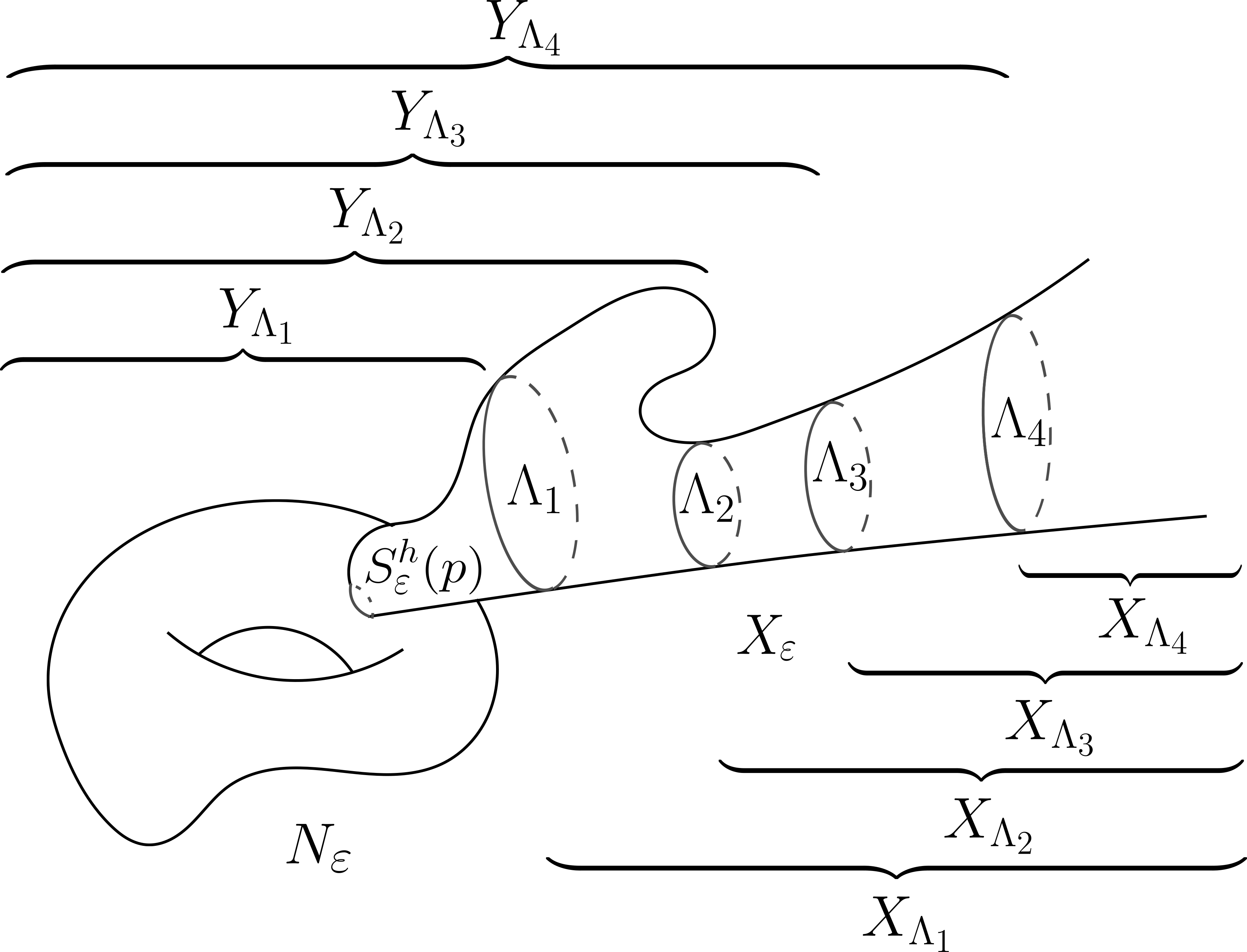
Figure 4. Avoidance hypersurfaces

3.2.2. Intersect at most one avoidance hypersurface

Setting $\tilde{\Lambda}_{2,i}$ as our avoidance hypersurfaces, we have

Proposition 3.4.

Let $\Sigma$ be a smoothly embedded, connected closed surface or curve in $(\tilde{Y},\tilde{g})$ with the induced metric $g_{\Sigma}$. Suppose that $\Sigma$ has $\mathbb{T}^{l}$-stablized scalar curvature $R$ which is greater than $R(\tilde{g})|_{\Sigma}-\delta_{1}$, where $\delta_{1}$ is the constant in Subsection 3.2.1. Then either we have

$$\Sigma\cap\tilde{X}_{\Lambda_{2}}=\emptyset$$

or there is a unique index $i_{0}$ such that

$$\Sigma\cap\tilde{X}_{\Lambda_{2}}\subset\tilde{X}_{\Lambda_{2},i_{0}}.$$

Proof.

It suffices to rule out the possibility that $\Sigma$ intersects with more than one components of $\tilde{X}_{\Lambda_{2}}$. Suppose by contradiction that $\Sigma$ intersects with $\tilde{X}_{\Lambda_{2},i_{1}}$ and $\tilde{X}_{\Lambda_{2},i_{2}}$ where $i_{1}\neq i_{2}$. Let $\tilde{\rho}_{i_{1}}$ be the short function from Lemma 2.4. From the construction we see $\tilde{\rho}_{i_{1}}<-T_{1}$ in $\tilde{X}_{\Lambda_{2},i_{1}}$ and $\tilde{\rho}_{i_{1}}>T_{1}$ in $\tilde{X}_{\Lambda_{2},i_{2}}$. Combining this with our assumption we see that $\tilde{\rho}_{i_{1}}(\Sigma)$ contains a neighborhood of the interval $[-T_{1},T_{1}]$. This allows us to pick up a value $c>T_{1}$ such that

$$V:=\Sigma\cap\tilde{\rho}_{i_{1}}^{-1}([-c,c])$$

is a smooth Riemannian band with $\partial V=\partial_{-}\cup\partial_{+}$, where $\partial_{-}=\tilde{\rho}_{i_{1}}^{-1}(-c)$ and $\partial_{+}=\tilde{\rho}_{i_{1}}^{-1}(c)$ are both non-empty and smooth. Let $h_{1}$ be the function from the definition of avoidance hypersurfaces and we take

$$h:\mathring{V}\to\mathbb{R},\quad h(x)=h_{1}\left(c^{-1}T_{1}\tilde{\rho}_{i_{1}}(x)\right).$$

We divide the discussion into the following two cases.

Case 1. $\Sigma$ is a surface. With the same proof as in Lemma 2.13 we can find a closed curve $\gamma$ in $\Sigma$ such that $\gamma$ has $\mathbb{T}^{l+1}$-stablized scalar curvature $R^{\prime}$ satisfying

$$R^{\prime}\geq R+(h_{1}^{2}-2|\mathrm{d}h_{1}|)\circ\tilde{\rho}_{i_{1}}>R(\tilde{g})|_{\gamma}+(h_{1}^{2}-2|\mathrm{d}h_{1}|)\circ\tilde{\rho}_{i_{1}}-\delta_{1}.$$

Recall that we have $\tilde{\rho}_{i_{1}}^{-1}([-d_{\Lambda_{1}},d_{\Lambda_{1}}])\subset\tilde{Y}_{\Lambda_{1}}$. This implies

$$R(\tilde{g})|_{\gamma}+(h_{1}^{2}-2|\mathrm{d}h_{1}|)\circ\tilde{\rho}_{i_{1}}\geq\left(\underline{R}_{1}\chi_{[-d_{\Lambda_{1}},d_{\Lambda_{1}}]}+h_{1}^{2}-2|\mathrm{d}h_{1}|\right)\circ\tilde{\rho}_{i_{1}}\geq\delta.$$

So we obtain $R^{\prime}>0$ but this contradicts the fact that $\mathbb{T}^{n}$ cannot admit any smooth metric with positive scalar curvature.

Case 2. $\Sigma$ is a curve. In this case, we must have $l\geq 1$. Then we can interprete the situation as the case that $V\times\mathbb{S}^{1}$ has $\mathbb{T}^{l-1}$-stablized scalar curvature $R$ which is greater than ${R(\tilde{g})|_{\Sigma}}-\delta_{1}$ and then deduce a contradiction as in the surface case. ∎

An analogous result holds for surfaces with boundary, where we use $\tilde{\Lambda}_{4,i}$ as the avoidance hypersurfaces:

Proposition 3.5.

Let $(\Sigma,\partial\Sigma)$ be a smoothly embedded, connected surface with boundary in $(\tilde{Y},\tilde{g})$ with the induced metric $g_{\Sigma}$. Suppose that $(\Sigma,\partial\Sigma)$ has $\mathbb{T}^{l}$-stablized scalar-mean curvature $(R,H)$ such that $R\geq R(\tilde{g})|_{\Sigma}-\delta_{2}$ and $H\geq 0$, where $\delta_{2}$ is the constant in Subsection 3.2.1. Then either we have

$$\Sigma\cap\tilde{X}_{\Lambda_{4}}=\emptyset$$

or there is a unique index $i_{0}$ such that

$$\Sigma\cap\tilde{X}_{\Lambda_{4}}\subset\tilde{X}_{\Lambda_{4},i_{0}}$$

and that each component of $\partial\Sigma$ has non-empty intersection with $\tilde{X}_{\Lambda_{2},i_{0}}$.

Proof.

The proof for $\Sigma$ not touching two components of $\tilde{X}_{\Lambda_{4}}$ follows the same argument as in the proof of Proposition 3.4. It remains to show that if $\Sigma$ intersects some component $\tilde{X}_{\Lambda_{4},i_{0}}$ then all the boundary components of $\Sigma$ have to intersect $\tilde{X}_{\Lambda_{2},i_{0}}$. Suppose by contradiction that there is a boundary component disjoint from $\tilde{X}_{\Lambda_{2},i_{0}}$, which we denote by $\partial_{-}$. We take $\tilde{\rho}$ to be the lift of the function $\rho_{\Lambda_{2}}$ on $\tilde{X}_{\Lambda_{2},i_{0}}$ and extend it to the whole $\tilde{Y}$ by zero extension. Since $\Sigma$ touches $\tilde{X}_{\Lambda_{4},i_{0}}$, the image of $\tilde{\rho}|_{\Sigma}$ must contain $[0,c]$ for some $c>T_{2}$. Without loss of generality we may assume $c$ to be a regular value of both $\tilde{\rho}|_{\Sigma}$ and $\tilde{\rho}|_{\partial\Sigma}$, and so $\tilde{\rho}^{-1}(c)\cap\Sigma$ is a smooth curve in $\Sigma$ which intersects $\partial\Sigma$ transversely. Take

$$\mathcal{N}=\tilde{\rho}^{-1}\left(\left(\frac{c+T_{2}}{2},c\right]\right)\cap\Sigma.$$

From the proof of Lemma 2.16 we can deform $\tilde{\rho}^{-1}(c)\cap\Sigma$ a little bit to find a curve contained in $\mathcal{N}$ which intersects $\partial\Sigma$ in acute angles. We denote this curve by $\partial_{+}$, and we denote the relative region on $\Sigma$ bounded by $\partial_{+}$ and $\partial_{-}$ relative to $\partial\Sigma$ by $V$. Notice that $\partial_{+}$ is contained in $\mathcal{N}$ where $\tilde{\rho}$-values are greater than $T_{2}$, so we can modify the function $\tilde{\rho}|_{V}$ to a new smooth function $\rho:V\to[0,T_{2}]$ such that

• $\rho=0$ on $\partial_{-}$ and $\rho^{-1}(T_{2})=\partial_{+}$;

• $\rho^{-1}([0,d_{\Lambda_{2}}])=(\tilde{\rho}|_{V})^{-1}([0,d_{\Lambda_{2}}])$;

• $\operatorname{Lip}\rho<1$.

Such function $\rho$ can be constructed by first using composition $\eta\circ\tilde{\rho}|_{V}$ with suitable function $\eta$ to change values greater than $T_{2}$ into a constant and then adding a function in the form of $c-\zeta\circ\operatorname{dist}(\cdot,\partial_{+})$ for suitable constant $c$ and function $\zeta$.

Take $h=h_{2}\circ\rho$, where $h_{2}$ is the function from the definition of avoidance hypersurfaces. With the same proof as in Lemma 2.14 we can find a curve $\gamma$ in $V$ such that $(\gamma,\partial\gamma)$ has $\mathbb{T}^{l+1}$-stablized scalar-mean curvature $(R^{\prime},H^{\prime})$ satisfying $H^{\prime}=H\geq 0$ and

$$R^{\prime}\geq R+(h_{2}^{2}-2|\mathrm{d}h_{2}|)\circ\rho>R(\tilde{g})|_{\gamma}+(h_{2}^{2}-2|\mathrm{d}h_{2}|)\circ\rho-\delta_{2}.$$

Recall that we have $\rho^{-1}([0,d_{\Lambda_{2}}])=(\tilde{\rho}|_{V})^{-1}([0,d_{\Lambda_{2}}])\subset\tilde{Y}_{\Lambda_{3}}$. This implies

$$R(\tilde{g})|_{\gamma}+(h_{2}^{2}-2|\mathrm{d}h_{2}|)\circ\rho\geq\left(\underline{R}_{2}\chi_{[0,d_{\Lambda_{2}}]}+h_{2}^{2}-2|\mathrm{d}h_{2}|\right)\circ\rho\geq\delta$$

and so we obtain $R^{\prime}>0$. However, it is impossible to have $R^{\prime}>0$ and $H\geq 0$ because otherwise by doubling trick one can construct a smooth metric on $\mathbb{T}^{l+2}$ with positive scalar curvature and this leads to a contradiction. ∎

3.3. Extrinsic diameter estimate

Let $M_{n-2}$ be the $(n-2)$-dimensional submanifold from Lemma 3.3. In the following, we take

$$\underline{R}=\min_{Y_{\Lambda_{4}}}R(g)$$

and

$$\mu_{\mathrm{loss}}=\frac{3}{4}\min\{\underline{R},\delta_{1},\delta_{2}\},$$

where $\mu_{\mathrm{loss}}$ is the constant in Lemma 3.3 and $\delta_{1}$ and $\delta_{2}$ are the constants from Subsection 3.2.1. Note that all these constants are positive.

3.3.1. Diameter estimate in dimensions three and four

When $n=3$ or $4$, we can bound the diameter of each component of $M_{n-2}$ that intersects $\tilde{Y}_{\Lambda_{2}}$.

Lemma 3.6.

Let $n=3$. For each component $C$ of $M_{n-2}$ with

$$C_{\Lambda_{2}}:=C\cap\tilde{Y}_{\Lambda_{2}}\neq\emptyset,$$

we have $C\cap\tilde{X}_{\Lambda_{2}}\neq\emptyset$ and

$$\operatorname{diam}(C_{\Lambda_{2}}\subset(\tilde{Y},\tilde{g}))\leq\frac{8\pi}{\sqrt{\underline{R}}}+\operatorname{diam}(\Lambda_{2}\subset(X_{\varepsilon},g)).$$

Proof.

Recall from Lemma 3.3 that $M_{n-2}$ has $\mathbb{T}^{2}$-stablized scalar curvature $R_{n-2}$ satisfying

$$R_{n-2}\geq R(\tilde{g})|_{M_{n-2}}-\mu_{\mathrm{loss}}>R(\tilde{g})|_{M_{n-2}}-\delta_{1}.$$

For each component $C$ of $M_{n-2}$ it follows from Proposition 3.4 that either $C\cap\tilde{X}_{\Lambda_{2}}=\emptyset$ or $C\cap\tilde{X}_{\Lambda_{2}}\subset\tilde{X}_{\Lambda_{2},i_{0}}$ for some uniquely determined $i_{0}=i_{0}(C)$.

In the former case, we see

$$R_{n-2}|_{C}\geq R(\tilde{g})|_{C}-\mu_{\mathrm{loss}}\geq\frac{1}{4}\underline{R}.$$

Since $C$ is one-dimensional, it is a closed curve. This leads to a contradiction since $\mathbb{T}^{3}$ cannot admit any smooth metric with positive scalar curvature.

In the latter case, we decompose $C_{\Lambda_{2}}:=C\cap\tilde{Y}_{\Lambda_{2}}$ into the union of its connected components

$$C_{\Lambda_{2}}=\bigcup_{i}U_{i}.$$

For each component $U_{i}$ we conclude from Lemma 2.16 that $r_{\mathrm{in}}(U_{i},\partial U_{i})\leq 4\pi/\sqrt{\underline{R}}$. Recall that we have $\partial U_{i}\subset\tilde{\Lambda}_{2,i_{0}}$ from the fact $C\cap\tilde{X}_{\Lambda_{2}}\subset\tilde{X}_{\Lambda_{2},i_{0}}$. From the triangle inequality we have

$$\operatorname{diam}(C_{\Lambda_{2}}\subset(\tilde{Y},\tilde{g}))\leq\frac{8\pi}{\sqrt{\underline{R}}}+\operatorname{diam}(\tilde{\Lambda}_{2,i_{0}}\subset(\tilde{X}_{\varepsilon,i_{0}},\tilde{g})).$$

Notice that $(\tilde{X}_{\varepsilon,i_{0}},\tilde{g})$ is isometric to $(X_{\varepsilon},g)$. We obtain the desired estimate

$$\operatorname{diam}(C_{\Lambda_{2}}\subset(\tilde{Y},\tilde{g}))\leq\frac{8\pi}{\sqrt{\underline{R}}}+\operatorname{diam}(\Lambda_{2}\subset(X_{\varepsilon},g)),$$

and this completes the proof. ∎

Lemma 3.7.

Let $n=4$. For each component $C$ of $M_{n-2}$ with

$$C_{\Lambda_{2}}:=C\cap\tilde{Y}_{\Lambda_{2}}\neq\emptyset,$$

we have

$$\operatorname{diam}(C_{\Lambda_{2}}\subset(\tilde{Y},\tilde{g}))\leq\frac{8\pi}{\sqrt{\underline{R}}}+\operatorname{diam}(\Lambda_{2}\subset(X_{\varepsilon},g)).$$

Proof.

The proof is the same as that of Lemma 3.6, where the only difference is that $C\cap\tilde{X}_{\Lambda_{2}}$ can be possibly empty now. In this case we have from Corollary 2.17 that

$$\operatorname{diam}(C\subset(\tilde{Y},\tilde{g}))\leq\operatorname{diam}(C,g_{n-2})\leq\frac{4\pi}{\sqrt{\underline{R}}}.$$

Therefore the desired diameter estimate still holds. ∎

3.3.2. Slice-and-dice in dimension five

For $n=5$, it might hold that the diameter of each component of $M_{n-2}$ is unbounded. Thus we need to employ the slice-and-dice procedure of Chodosh–Li [5, Section 6]. We first slice $M_{n-2}$ into a manifold with boundary whose second homology comes from its boundary, and we then dice it so that the blocks after slice-and-dice have extrinsic diameter control.

Proposition 3.8.

Let $n=5$. If $M_{n-2}$ has non-empty intersection with $\tilde{Y}_{\Lambda_{2}}$, then for each component $C$ of $M_{n-2}$ we can construct a slice-and-dice of $C$ consisting of finitely many slicing surfaces $\{S_{i}\}$ and finitely many dicing surfaces $\{D_{j}\}$ such that

• $\{S_{i}\}$ are pairwisely disjoint closed surfaces satisfying

  $$\operatorname{diam}(S_{i,\Lambda_{2}}\subset(\tilde{Y},\tilde{g}))\leq\frac{8\pi}{\sqrt{\underline{R}}}+\operatorname{diam}(\Lambda_{2}\subset(X_{\varepsilon},g)),$$

  where $S_{i,\Lambda_{2}}:=S_{i}\cap\tilde{Y}_{\Lambda_{2}}$;

• $\{D_{j}\}$ are pairwisely disjoint surfaces satisfying

  $$\operatorname{diam}(D_{j,\Lambda_{4}}\subset(\tilde{Y},\tilde{g}))\leq\frac{16\pi}{\sqrt{\underline{R}}}+\operatorname{diam}(\Lambda_{4}\subset(X_{\varepsilon},g)),$$

  where $D_{j,\Lambda_{4}}:=D_{j}\cap\tilde{Y}_{\Lambda_{4}}$. Furthermore, if $D_{j}\cap\tilde{X}_{\Lambda_{4}}=\emptyset$, then $D_{j}$ is a topological sphere or disk.

• Decompose the complement of $\{S_{i}\}$ and $\{D_{j}\}$ as the union of its connected components

  $$C-\left(\bigcup_{i}S_{i}\right)\cup\left(\bigcup_{j}D_{j}\right)=\bigcup_{k}U_{k}.$$

  Then $U_{k,\Lambda_{2}}:=U_{k}\cap\tilde{Y}_{\Lambda_{2}}$ satisfies

  $$\begin{split}\operatorname{diam}(U_{k,\Lambda_{2}}\subset(\tilde{Y},\tilde{g}))&\leq\frac{40\pi}{\sqrt{\underline{R}}}+5\operatorname{diam}(\Lambda_{2}\subset(X_{\varepsilon},g))\\ &\qquad\qquad+2\operatorname{diam}(\Lambda_{4}\subset(X_{\varepsilon},g))+\frac{8\pi}{\sqrt{\hat{\mu}_{\mathrm{loss}}}}\end{split}$$

  with

  $$\hat{\mu}_{\mathrm{loss}}=\frac{3}{16}\min\{\underline{R},\delta_{1},\delta_{2}\}.$$

Proof.

The proof follows from the argument of Chodosh–Li [5, Section 6] (see also [35, Section 2]) with an essential improvement on the extrinsic diameter control of slicing surfaces, dicing surfaces and blocks after slice-and-dice. The proof will be divided into two steps.

Step 1. Slicing.

We are going to show that there are pairwisely disjoint embedded closed surfaces $S_{1},S_{2},\ldots,S_{i_{1}}$ satisfying

• the inclusion $i:H_{2}(\partial\hat{C})\to H_{2}(\hat{C})$ is surjective, where $\hat{C}$ is the metric completion of $C-\cup_{i}S_{i}$;

• and we have

  $$\operatorname{diam}(S_{i,\Lambda_{2}}\subset(\tilde{Y},\tilde{g}))\leq\frac{8\pi}{\sqrt{\underline{R}}}+\operatorname{diam}(\Lambda_{2}\subset(X_{\varepsilon},g)),$$

  where $S_{i,\Lambda_{2}}:=S_{i}\cap\tilde{Y}_{\Lambda_{2}}$.

Set $\hat{C}_{0}=C$. If $\hat{C}_{0}$ satisfies $H_{2}(\hat{C}_{0})=0$, then we are done. Otherwise $\hat{C}_{0}$ satisfies $H_{2}(\hat{C}_{0})\neq 0$ and we can fix a non-zero class $\beta_{1}\in H_{2}(\hat{C}_{0})$. Recall that $M_{n-2}$ has $\mathbb{T}^{2}$-stablized scalar curvature $R_{n-2}$ satisfying

$$R_{n-2}\geq R(\tilde{g})|_{M_{n-2}}-\mu_{\mathrm{loss}}.$$ (3.4)

The same thing holds for $\hat{C}_{0}$. It follows from Lemma 2.11 that there is an embedded surface $S$ with integer multiplicity such that $S$ has $\mathbb{T}^{3}$-stablized scalar curvature $R_{n-3}$ which is no less than $R_{n-2}|_{S}$ and the metric completion of $\hat{C}_{0}-S$ associated with its boundary has $\mathbb{T}^{2}$-stablized scalar-mean curvature $(R_{n-2},0)$. Just take one component of $S$ and we denote it by $S_{1}$.

Next we consider the metric completion $\hat{C}_{1}$ of $\hat{C}_{0}-S_{1}$. In a natural way, $(\hat{C}_{1},\partial\hat{C}_{1})$ has $\mathbb{T}^{2}$-stablized scalar-mean curvature $(R_{n-2},0)$ where $R_{n-2}$ is no less than $R(\tilde{g})|_{M_{n-2}}-\mu_{\mathrm{loss}}$. Similarly, if the map $H_{2}(\partial\hat{C}_{1})\to H_{2}(\hat{C}_{1})$ is surjective, then we are done. Otherwise, we can find an embedded surface $S_{2}$ representing a non-trivial class

$$\beta_{2}\in H_{2}(\hat{C}_{1})-\mathrm{Im}\left(H_{2}(\partial\hat{C}_{1})\to H_{2}(\hat{C}_{1})\right),$$

which has $\mathbb{T}^{3}$-stablized scalar curvature $R_{n-3}$ that is no less than $R_{n-2}|_{S_{2}}$ and the metric completion $(\hat{C}_{2},\partial\hat{C}_{2})$ of $\hat{C}_{1}-S_{2}$ has $\mathbb{T}^{2}$-stablized scalar-mean curvature are $(R_{n-2},0)$.

By induction we can construct a sequence of surfaces $\{S_{i}\}_{i\in I}$ satisfying

$$[S_{i}]\in H_{2}(\hat{C}_{i-1})-\mathrm{Im}\left(H_{2}(\partial\hat{C}_{i-1})\to H_{2}(\hat{C}_{i-1})\right)$$

and $S_{i}$ has $\mathbb{T}^{3}$-stablized scalar curvature $R_{n-3}$ which is no less than $R_{n-2}|_{S_{i}}$. Also, each $(\hat{C}_{i},\partial\hat{C}_{i})$ has $\mathbb{T}^{2}$-stablized scalar-mean curvature are $(R_{n-2},0)$.

Termination of the construction. We have to show that the construction terminates in finitely many steps. This comes from a topological argument by Bamler, Li and Mantoulidis (see the proof of [2, Lemma 2.5]) and here we write out the details for completeness. Denote $i_{k}:H_{2}(\partial\hat{C}_{k})\to H_{2}(\hat{C}_{k})$ and the goal is to show that the quotient $Q_{k}=H_{2}(\hat{C}_{k})/\mathrm{Im}\,i_{k}$ is torsion-free and has strictly decreasing rank when $k$ increases. To see that $Q_{k}$ is torsion-free we consider the exact sequence

$$H_{2}(\partial\hat{C}_{k})\to H_{2}(\hat{C}_{k})\to H_{2}(\hat{C}_{k},\partial\hat{C}_{k})\to H_{1}(\partial\hat{C}_{k}).$$

Recall that $\mathrm{dim}\,\hat{C}_{k}=3$ and so $H_{2}(\hat{C}_{k},\partial\hat{C}_{k})\cong H^{1}(\hat{C}_{k})$ is torsion-free. From the above exact sequence $Q_{k}$ is isometric to the image of $H_{2}(\hat{C}_{k})\to H_{2}(\hat{C}_{k},\partial\hat{C}_{k})$, which is a subgroup of $H_{2}(\hat{C}_{k},\partial\hat{C}_{k})$ and so is torsion-free. Next we show that the rank of $Q_{k}$ decreases strictly. Let $\mathcal{N}_{S_{k+1}}$ denote the tubular neighborhood of $S_{k+1}$ in $\hat{C}_{k}$. Consider the exact sequence

$$H_{2}(\partial\mathcal{N}_{S_{k+1}})\to H_{2}(\hat{C}_{k+1})\oplus H_{2}(\mathcal{N}_{S_{k+1}})\to H_{2}(\hat{C}_{k}).$$

It is clear that $\ker\big{(}H_{2}(\hat{C}_{k+1})\to H_{2}(\hat{C}_{k})\big{)}$ is contained in the image of $H_{2}(\partial\mathcal{N}_{S_{k+1}})\to H_{2}(\hat{C}_{k+1})$ and so contained in the image of $i_{k+1}$. This induces an injective map

$$Q_{k+1}\to H_{2}(\hat{C}_{k})/\mathrm{Im}\,i_{k+1}\cong Q_{k}/[S_{k+1}]$$

and so $\mathrm{rank}\,Q_{k+1}<\mathrm{rank}\,Q_{k}$.

Diameter bound for slicing surfaces. Recall that $\mu_{\mathrm{loss}}$ is no greater than $3\delta_{1}/{4}$. Then we can apply Proposition 3.4 to each $S_{i}$ so that we obtain either $S_{i}\cap\tilde{X}_{\Lambda_{2}}=\emptyset$ or $S_{i}\cap\tilde{X}_{\Lambda_{2}}\subset\tilde{X}_{\Lambda_{2},i_{0}}$ for a uniquely determined index $i_{0}=i_{0}(S_{i})$. In the former case, it follows from

$$R_{n-3}\geq R_{n-2}|_{S_{i}}\geq R(\tilde{g})|_{S_{i}}-\mu_{\mathrm{loss}}\geq\frac{1}{4}\underline{R}$$

and Corollary 2.17 that

$$\operatorname{diam}(S_{i,\Lambda_{2}}\subset(\tilde{Y},\tilde{g}))\leq\operatorname{diam}(S_{i},g_{S_{i}})\leq\frac{4\pi}{\sqrt{\underline{R}}}.$$

In the latter case, we write $S_{i,\Lambda_{2}}=\cup_{l}S_{il}$ as the decomposition into connected components. Clearly we have $\partial S_{il}\subset\tilde{\Lambda}_{2,i_{0}}$ from the fact $S_{i}\cap\tilde{X}_{\Lambda_{2}}\subset\tilde{X}_{\Lambda_{2},i_{0}}$. From Lemma 2.16 we see $r_{\mathrm{in}}(S_{il},\partial S_{il})\leq 4\pi/\sqrt{\underline{R}}$ and we obtain from the triangle inequality that

$$\operatorname{diam}(S_{i,\Lambda_{2}}\subset(\tilde{Y},\tilde{g}))\leq\frac{8\pi}{\sqrt{\underline{R}}}+\operatorname{diam}(\Lambda_{2}\subset(X_{\varepsilon},g)).$$

Step 2. Dicing.

Let $\hat{C}$ be the metric completion of $C-\cup_{i}S_{i}$. From the fact $C\cap\tilde{Y}_{\Lambda_{2}}\neq\emptyset$ we have $\hat{C}\cap\tilde{Y}_{\Lambda_{2}}\neq\emptyset$ as well. Fix a point $p\in\hat{C}\cap\tilde{Y}_{\Lambda_{2}}$ and take a small geodesic ball $B_{\delta}$ centered at $p$. By taking $\delta$ small enough we can guarantee $\partial B_{\delta}\cap\tilde{X}_{\Lambda_{2}}=\emptyset$ and

$$\operatorname{diam}(\partial B_{\delta}\subset(\tilde{Y},\tilde{g}))\leq\frac{16\pi}{\sqrt{\underline{R}}}+\operatorname{diam}(\Lambda_{4}\subset(X_{\varepsilon},g)).$$

Set

$$\hat{\mu}_{\mathrm{loss}}=\frac{3}{16}\min\{\underline{R},\delta_{1},\delta_{2}\}.$$

In the following, we divide the argument into two cases.

Case 1. The whole $\hat{C}$ is contained in the $(4\pi/\sqrt{\hat{\mu}_{\mathrm{loss}}})$-neighborhood of $\partial B_{\delta}$. By assumption for each point $q\in\hat{C}\cap\tilde{Y}_{\Lambda_{2}}$ we can find a curve $\gamma$ connecting $q$ and $\partial B_{\delta}$ with length no greater than $4\pi/\sqrt{\hat{\mu}_{\mathrm{loss}}}$. It follows from the diameter estimate of $\partial B_{\delta}$ and the triangle inequality that

$$\operatorname{diam}(\hat{C}\subset(\tilde{Y},\tilde{g}))\leq\frac{8\pi}{\sqrt{\hat{\mu}_{\mathrm{loss}}}}+\frac{8\pi}{\sqrt{\underline{R}}}+\operatorname{diam}(\Lambda_{4}\subset(X_{\varepsilon},g)).$$

Case 2. The complement $\hat{C}-B(B_{\delta};4\pi/\sqrt{\hat{\mu}_{\mathrm{loss}}})$ is non-empty. In this case, we have to construct suitable surfaces for dicing. For our purpose let us take the Riemannian band $(V,\partial_{\pm})$ coming from a smoothing

$$\bar{B}(B_{\delta};4\pi/\sqrt{\hat{\mu}_{\mathrm{loss}}})-B(B_{\delta};\pi/\sqrt{\hat{\mu}_{\mathrm{loss}}})$$

such that $\operatorname{dist}(\partial_{+},\partial_{-})>2\pi/\sqrt{\hat{\mu}_{\mathrm{loss}}}$. With the same deformation argument as the one at the end of the proof of Lemma 2.16, we can further assume that $\partial_{+}\cup\partial_{-}$ intersects with $\overline{\partial V-(\partial_{+}\cup\partial_{-})}$ in acute angles. By construction,$(\hat{C},\partial\hat{C})$ has $\mathbb{T}^{2}$-stablized scalar-mean curvature $(R_{n-2},0)$ and the same thing holds for $(V,\overline{\partial V-(\partial_{+}\cup\partial_{-})})$. Now it follows from Lemma 2.14 and (3.4) that we can find a surface $\Sigma$ bounding a region with $\partial_{-}$ such that $(\Sigma,\partial\Sigma)$ has $\mathbb{T}^{3}$-stablized scalar-mean curvature $(R_{n-3}^{\prime},H_{n-3}^{\prime})$ satisfying

$$R_{n-3}^{\prime}\geq R(\tilde{g})|_{\Sigma}-\mu_{\mathrm{loss}}-\hat{\mu}_{\mathrm{loss}}\mbox{ and }H_{n-3}^{\prime}=0.$$

Clearly $\Sigma$ bounds a relative region $\Omega_{1}$ containing $B_{\delta}$ relative to $\partial\hat{C}$. Since $\Omega_{1}$ may have multiple components, we take the component of $\Omega_{1}$ containing $B_{\delta}$, still denoted by $\Omega_{1}$.

With $B_{\delta}$ replaced by $\Omega_{1}$ we can repeat the above construction and inductively we end up with an exhaustion

$$B_{\delta}=\Omega_{0}\subset\Omega_{1}\subset\Omega_{2}\subset\cdots\subset\Omega_{m}\subset\hat{C},$$

where each $\Omega_{k}$ is connected and the finiteness of this exhaustion comes from the facts

$$B(B_{\delta},\pi k/\sqrt{\hat{\mu}_{\mathrm{loss}}})\subset\Omega_{k}$$

and that $\hat{C}$ has bounded diameter from its compactness. For each $\Omega_{k}$ its reduced boundary $\partial\Omega_{k}\cap\mathring{\hat{C}}$ has $\mathbb{T}^{3}$-stablized scalar-mean curvature $(R_{n-3}^{\prime},H_{n-3}^{\prime})$ satisfying

$$R_{n-3}^{\prime}\geq R(\tilde{g})|_{\Sigma}-\mu_{\mathrm{loss}}-\hat{\mu}_{\mathrm{loss}}\mbox{ and }H_{n-3}^{\prime}=0.$$

The dicing surfaces $D_{j}$ are taken to be components of the induced boundaries $\partial\Omega_{k}\cap\mathring{\hat{C}}$.

Diameter bound for dicing surfaces. Recall that we have

$$\mu_{\mathrm{loss}}+\hat{\mu}_{\mathrm{loss}}\leq\frac{15}{16}\delta_{2}.$$

So we can apply Proposition 3.5 to each dicing surface $D_{j}$ and conclude that either $D_{j}\cap\tilde{X}_{\Lambda_{4}}=\emptyset$ or there is a uniquely determined index $i_{0}^{\prime}$ such that $D_{j}\cap\tilde{X}_{\Lambda_{4}}\subset\tilde{X}_{\Lambda_{4},i_{0}^{\prime}}$. In the former case, we conclude from Corollary 2.17, $R_{n-3}^{\prime}\geq\underline{R}/16$ and $H_{n-3}^{\prime}=0$ that $D_{j}$ is a topological sphere or disk and

$$\operatorname{diam}(D_{j,\Lambda_{4}}\subset(\tilde{Y},\tilde{g}))\leq\operatorname{diam}(D_{j})\leq\frac{8\pi}{\sqrt{\underline{R}}},\mbox{ where }D_{j,\Lambda_{4}}:=D_{j}\cap\tilde{Y}_{\Lambda_{4}}.$$

In the latter case, we write $D_{j,\Lambda_{4}}=\cup_{l}D_{jl}$ where $D_{jl}$ are components of $D_{j,\Lambda_{4}}$ with $\partial D_{jl}-\partial D_{j}\subset\tilde{\Lambda}_{4,i_{0}^{\prime}}$. It follows from Lemma 2.16 and the triangle inequality that

$$\operatorname{diam}(D_{j,\Lambda_{4}}\subset(\tilde{Y},\tilde{g}))\leq\frac{16\pi}{\sqrt{\underline{R}}}+\operatorname{diam}(\Lambda_{4}\subset(X_{\varepsilon},g)).$$

Diameter bound for blocks. Decompose the complement of $\{S_{i}\}$ and $\{D_{j}\}$ into its connected components as

$$C-\left(\bigcup_{i}S_{i}\right)\cup\left(\bigcup_{j}D_{j}\right)=\bigcup_{k}U_{k}.$$

We are going to estimate the extrinsic diameter bound for $U_{k,\Lambda_{2}}:=U_{k}\cap\tilde{X}_{\Lambda_{2}}$.

First we need to prove the following key lemma.

Lemma 3.9.

Let $\Gamma$ be a connected component of the total slice-and-dice set

$$\mathcal{T}_{SD}:=\left(\bigcup_{i}S_{i}\right)\cup\left(\bigcup_{j}D_{j}\right).$$

Then we have

$$\operatorname{diam}(\Gamma_{\Lambda_{2}}\subset(\tilde{Y},\tilde{g}))\leq\frac{40\pi}{\sqrt{\underline{R}}}+3\operatorname{diam}(\Lambda_{2}\subset(X_{\varepsilon},g))+2\operatorname{diam}(\Lambda_{4}\subset(X_{\varepsilon},g)),$$

where $\Gamma_{\Lambda_{2}}:=\Gamma\cap\tilde{Y}_{\Lambda_{2}}$.

Proof.

Notice that $\Gamma$ has the structure of a graph where each vertex corresponds to a slicing surface or a dicing surface, and there is an edge between two vertices if the two surfaces representing the vertices have non-empty intersection. After marking each vertex by $\mathcal{S}$ or $\mathcal{D}$ to record its source from slicing surfaces or dicing surfaces, we know from the construction that each edge must be of $\mathcal{S}$-$\mathcal{D}$ type. To obtain a diameter bound of $\Gamma_{\Lambda_{2}}$ we just need to estimate a uniform diameter bound of $\Gamma_{0,\Lambda_{2}}:=\Gamma_{0}\cap\tilde{Y}_{\Lambda_{2}}$ for any path-structured “subcomplex” $\Gamma_{0}$ of $\Gamma$.

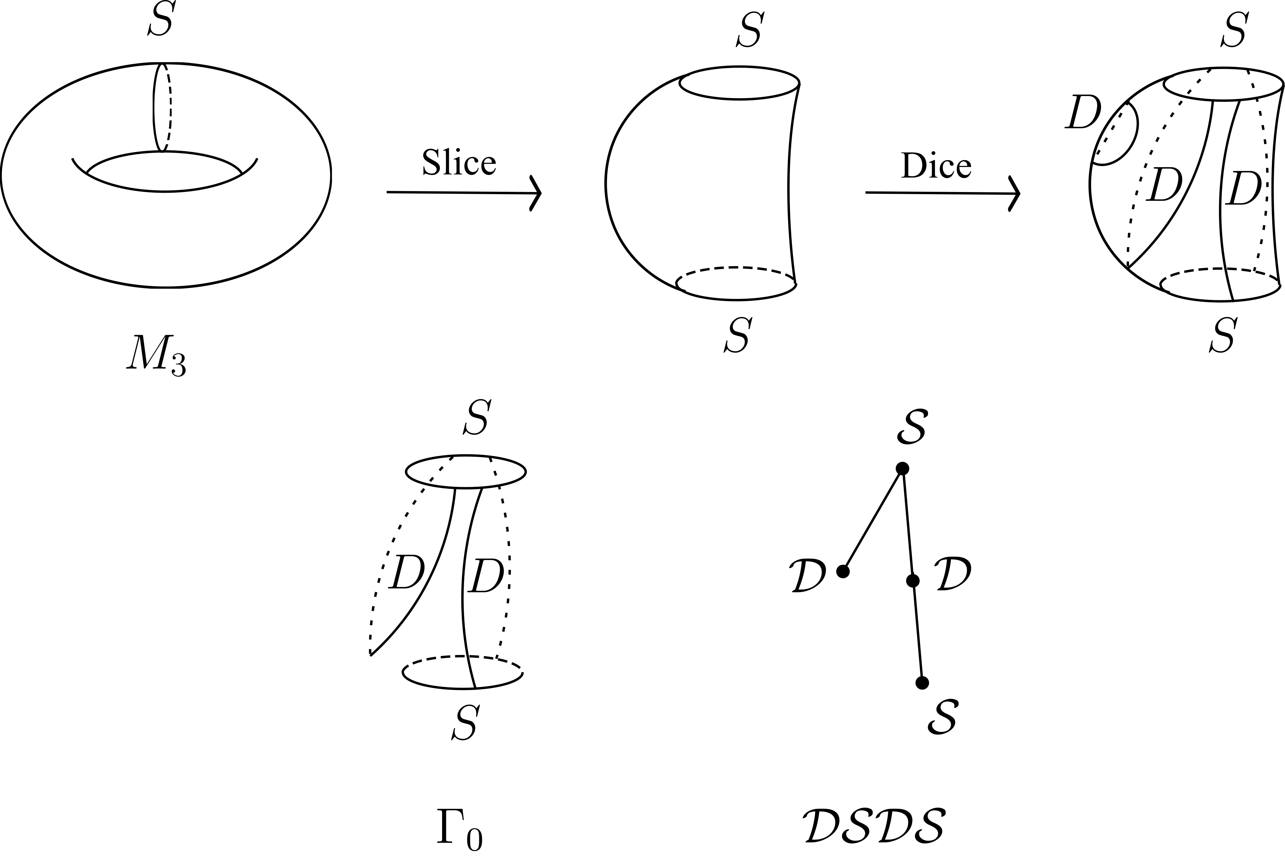
Figure 5. The graph structure of this path-structured “subcomplex” $\Gamma_{0}$ is $\mathcal{DSDS}$

We begin with the following observation: there are at most two dicing surfaces in $\Gamma_{0}$ disjoint from $\tilde{X}_{\Lambda_{4}}$. In order to see this we recall that if a dicing surface $D_{j}$ is disjoint from $\tilde{X}_{\Lambda_{4}}$, then it has to be a topological sphere or disk. In the former case, $\Gamma_{0}$ is a single dicing sphere and we obtain the required diameter estimate

$$\operatorname{diam}(\Gamma_{0,\Lambda_{2}})\leq\frac{8\pi}{\sqrt{\underline{R}}}.$$

In the latter case, since a dicing disk has only one boundary component and thus can only intersect exactly one slicing surface, it must lie in the end-point position of the path structure corresponding to $\Gamma_{0}$. Thus the number of dicing disks in $\Gamma_{0}$ cannot exceed two, establishing our observation. After removing the (at most two) dicing surfaces in the end-point position of $\Gamma_{0}$, we obtain a reduced “subcomplex” $\Gamma_{0}^{\prime}$ which has the path structure of the type $\mathcal{S}\mathcal{D}\mathcal{S}\mathcal{D}\cdots\mathcal{S}$, where each dicing surface intersects with some $\tilde{X}_{\Lambda_{4},i}$. When there is no $\mathcal{D}$-component (i.e. $\Gamma_{0}^{\prime}$ consists of a single slicing surface), we obtain the required diameter estimate

$$\operatorname{diam}(\Gamma_{0,\Lambda_{2}}^{\prime}\subset(\tilde{Y},\tilde{g}))\leq\frac{16\pi}{\sqrt{\underline{R}}}+\operatorname{diam}(\Lambda_{2}\subset(X_{\varepsilon},g)).$$

Otherwise, we claim that all dicing surfaces in $\Gamma_{0}^{\prime}$ must intersect the same $\tilde{X}_{\Lambda_{4},i_{0}}$. Clearly we are done if there is only one $\mathcal{D}$-component, so we just need to deal with the case when there are at least two $\mathcal{D}$-components. For our purpose, we take a closer look at the $\mathcal{D}\mathcal{S}\mathcal{D}$-structure with two dicing surfaces involved. Recall that if a dicing surface $D_{j}$ intersects some $\tilde{X}_{\Lambda_{4},i}$ then every component of $\partial D_{j}$ must intersect $\tilde{X}_{\Lambda_{2},i}$ with the same index $i$. Combining the fact that a slicing surface can only intersect one $\tilde{X}_{\Lambda_{2},i}$, we conclude that adjacent dicing surfaces in $\Gamma_{0}^{\prime}$ must intersect the same $\tilde{X}_{\Lambda_{4},i_{0}}$ for some index $i_{0}$ and consequently all dicing surfaces in $\Gamma_{0}^{\prime}$ intersect the same $\tilde{X}_{\Lambda_{4},i_{0}}$. As a consequence, every slicing surface in $\Gamma_{0}^{\prime}$ must intersect $\tilde{X}_{\Lambda_{2},i_{0}}$ since it contains some boundary component of the dicing surfaces.

Take any pair of points $p,q\in\Gamma_{0,\Lambda_{2}}^{\prime}$. Then we can find two surfaces $\Sigma_{1}$ and $\Sigma_{2}$ in $\Gamma_{0}^{\prime}$ such that $p\in\Sigma_{1,\Lambda_{2}}:=\Sigma_{1}\cap\tilde{Y}_{\Lambda_{2}}$ and $q\in\Sigma_{2,\Lambda_{2}}:=\Sigma_{2}\cap\tilde{Y}_{\Lambda_{2}}$. From our previous discussion we can find a point $p^{*}$ in $\Sigma_{1}\cap\tilde{\Lambda}_{2,i_{0}}$ and a point $q^{*}$ in $\Sigma_{2}\cap\tilde{\Lambda}_{2,i_{0}}$. Then we have

$$\begin{split}\operatorname{dist}(p,q)&\leq\operatorname{dist}(p,p^{*})+\operatorname{dist}(p^{*},q^{*})+\operatorname{dist}(q^{*},q)\\ &\leq\frac{32\pi}{\sqrt{\underline{R}}}+3\operatorname{diam}(\Lambda_{2}\subset(X_{\varepsilon},g))+2\operatorname{diam}(\Lambda_{4}\subset(X_{\varepsilon},g)).\end{split}$$

Since $p$ and $q$ are chosen arbitrarily, we have the same bound for the extrinsic diameter $\operatorname{diam}(\Gamma_{0,\Lambda_{2}}^{\prime}\subset(\tilde{Y},\tilde{g}))$. Recall that $\Gamma_{0}$ and $\Gamma_{0}^{\prime}$ differ by at most two slicing disks with diameter bounded by $8\pi/\sqrt{\underline{R}}$, we conclude

$$\operatorname{diam}(\Gamma_{0,\Lambda_{2}}\subset(\tilde{Y},\tilde{g}))\leq\frac{40\pi}{\sqrt{\underline{R}}}+3\operatorname{diam}(\Lambda_{2}\subset(X_{\varepsilon},g))+2\operatorname{diam}(\Lambda_{4}\subset(X_{\varepsilon},g)).$$

The proof is completed by noticing that any pair of points $p,q\in\Gamma_{\Lambda_{2}}$ can be realized as a pair of points in some $\Gamma_{0,\Lambda_{2}}$ for some “subcomplex” $\Gamma_{0}$ with path structure. ∎

Now we are ready to give diameter estimates for blocks $U_{k}$. Let $U_{k}$ be the block obtained from the $l$-th dicing, namely a component of $\Omega_{l}-\Omega_{l-1}$. Recall that from our construction of the dicing surfaces in Step 2, every point in $U_{k}$ has distance no greater than $4\pi/\sqrt{\hat{\mu}_{\mathrm{loss}}}$ from $\partial\Omega_{l-1}\cap\partial U_{k}$. Thus, to obtain a diameter estimate of $U_{k}$, it suffices to bound $\partial\Omega_{l-1}\cap\partial U_{k}$. For this end, we denote the components of $\partial\Omega_{l-1}\cap\partial U_{k}$ by $D_{k1},D_{k2},\ldots,D_{km}$. We divide the discussion into the following two cases:

Case 1. $m=1$. If we have $D_{k1}\cap\tilde{X}_{\Lambda_{4}}=\emptyset$, then

$$\operatorname{diam}(U_{k}\subset(\tilde{Y},\tilde{g}))\leq\operatorname{diam}(D_{k1})+\frac{8\pi}{\sqrt{\hat{\mu}_{\mathrm{loss}}}}\leq\frac{8\pi}{\sqrt{\underline{R}}}+\frac{8\pi}{\sqrt{\hat{\mu}_{\mathrm{loss}}}}.$$

Otherwise, we consider the set

$$\mathcal{K}=D_{k1,\Lambda_{4}}\cup\left(\bigcup_{i:D_{k1}\cap\tilde{X}_{\Lambda_{4},i}\neq\emptyset}\tilde{\Lambda}_{4,i}\right),$$

where $D_{k1,\Lambda_{4}}=D_{k1}\cap\tilde{Y}_{\Lambda_{4}}$. Clearly we have that

• when $D_{k1}$ is completely contained in some $\tilde{X}_{\Lambda_{4},i}$, we have $\mathcal{K}=\tilde{\Lambda}_{4,i}$ and so $\operatorname{diam}(\mathcal{K}\subset(\tilde{Y},\tilde{g}))\leq\operatorname{diam}(\Lambda_{4}\subset(X_{\varepsilon},g))$;

• otherwise $D_{k1,\Lambda_{4}}\neq\emptyset$ and so $D_{k1}\cap\tilde{\Lambda}_{4,i}\neq\emptyset$ for each index $i$ satisfying $D_{k1}\cap\tilde{X}_{\Lambda_{4},i}\neq\emptyset$. From the triangle inequality we conclude

  $$\begin{split}\operatorname{diam}(\mathcal{K}\subset(\tilde{Y},\tilde{g}))&\leq 2\operatorname{diam}(\Lambda_{4}\subset(X_{\varepsilon},g))+\operatorname{diam}(D_{k1,\Lambda_{4}}\subset(\tilde{Y},\tilde{g}))\\ &=\frac{16\pi}{\sqrt{\underline{R}}}+3\operatorname{diam}(\Lambda_{4}\subset(X_{\varepsilon},g)).\end{split}$$

Given any point $p$ in $U_{k,\Lambda_{4}}$ we can connect $p$ and $D_{k1}$ by a curve $\gamma$ with length no greater than $4\pi/\sqrt{\hat{\mu}_{\mathrm{loss}}}$ by our construction. Notice that $\gamma$ must intersect with $\mathcal{K}$. From the triangle inequality we obtain

$$\operatorname{diam}(U_{k,\Lambda_{4}}\subset(\tilde{Y},\tilde{g}))\leq\frac{16\pi}{\sqrt{\underline{R}}}+\frac{8\pi}{\sqrt{\hat{\mu}_{\mathrm{loss}}}}+3\operatorname{diam}(\Lambda_{4}\subset(X_{\varepsilon},g)).$$

Case 2. $m\geq 2$. We claim that each $D_{ki}$ must intersect at least one slicing surface. If not, we can find a simple closed curve $\gamma$ in $\hat{C}$ which intersects only once with $D_{ki}$. This implies that $D_{ki}$ represents a non-trivial homology class in $H_{2}(\hat{C})$, which does not lie in the image of $H_{2}(\partial\hat{C})\to H_{2}(\hat{C})$. This contradicts the surjectivity of $H_{2}(\partial\hat{C})\to H_{2}(\hat{C})$ from the construction in the slicing procedure in Step 1.

Now we collect all the slicing surfaces intersecting $D_{ki}$ and denote them by $S_{k1},S_{k2},\ldots,S_{kl}$. We claim that the union

$$\mathcal{T}_{k}:=\left(\bigcup_{i=1}^{m}D_{ki}\right)\cup\left(\bigcup_{j=1}^{l}S_{kj}\right)$$

must lie in some component of the total slice-and-dice set

$$\mathcal{T}_{SD}:=\left(\bigcup_{i}S_{i}\right)\cup\left(\bigcup_{j}D_{j}\right).$$

Otherwise, $D_{ki}$ and $S_{kj}$ can be divided into $s\geq 2$ collections

$$\mathcal{B}_{\tau}=\{D_{k1}^{\tau},\ldots,D_{km_{\tau}}^{\tau},S_{k1}^{\tau},\ldots,D_{kl_{\tau}}^{\tau}\},\,\tau=1,2,\ldots,s,$$

such that the unions of $D_{ki}$ and $S_{kj}$ from different collections lie in different components of $\mathcal{T}_{SD}$. For the first collection we notice that the combination of chains

$$D_{k1}^{1}+\cdots+D_{km_{1}}^{1}-(\partial\Omega_{l-1})\cap\left(\bigcup_{j=1}^{l_{1}}S_{kj}^{1}\right)$$

turns out to be a cycle in $\hat{C}$. Since there are other dicing surfaces from the second collection, as before we can construct a simple closed curve in the interior of $\hat{C}$ which only intersects once with the above cycle, which yields a contradiction to the surjectivity of $H_{2}(\partial\hat{C})\to H_{2}(\hat{C})$ again.

From previous discussion we can conclude from Lemma 3.9 that

$$\operatorname{diam}(\mathcal{T}_{k,\Lambda_{2}}\subset(\tilde{Y},\tilde{g}))\leq\frac{40\pi}{\sqrt{\underline{R}}}+3\operatorname{diam}(\Lambda_{2}\subset(X_{\varepsilon},g))+2\operatorname{diam}(\Lambda_{4}\subset(X_{\varepsilon},g)).$$

From a similar discussion as in Case 1 depending on $\mathcal{T}_{k}\cap\tilde{X}_{\Lambda_{2}}$ empty or not we can obtain

$$\begin{split}\operatorname{diam}(U_{k,\Lambda_{2}}\subset(\tilde{Y},\tilde{g}))&\leq\frac{40\pi}{\sqrt{\underline{R}}}+5\operatorname{diam}(\Lambda_{2}\subset(X_{\varepsilon},g))\\ &\qquad\qquad+2\operatorname{diam}(\Lambda_{4}\subset(X_{\varepsilon},g))+\frac{8\pi}{\sqrt{\hat{\mu}_{\mathrm{loss}}}}.\end{split}$$

This completes the proof. ∎

3.4. Completion of the proof of Theorem 1.2

First we present a quantitative filling lemma for $M_{n-2}$.

Proposition 3.10.

Let $n\in\{3,4,5\}$. Assume that $M_{n-2}\cap\tilde{N}_{\varepsilon}\neq\emptyset$. There is a positive constant $r_{0}$ independent of $L$ such that $M_{n-2}$ can be realized as the relative boundary of a chain $\Gamma$ relative to $\tilde{X}_{\varepsilon}$, whose support is contained in $B^{\tilde{g}}_{r_{0}}(M_{n-2})$.

Proof.

It suffices to deal with each component $C$ of $M_{n-2}$.

Dimension three and four. It follows from Lemma 2.7 that we have $[C]=0\in H_{n-2}(\tilde{Y},\tilde{X}_{\varepsilon})$ and so the same thing holds for $C_{\varepsilon}:=C\cap\tilde{N}_{\varepsilon}$. From Lemma 3.6 and Lemma 3.7 we see

$$\operatorname{diam}(C_{\varepsilon}\subset(\tilde{Y},\tilde{g}))\leq\operatorname{diam}(C_{\Lambda_{2}}\subset(\tilde{Y},\tilde{g}))\leq r_{1}^{*},$$

where

$$r_{1}^{*}=\frac{8\pi}{\sqrt{\underline{R}}}+\operatorname{diam}(\Lambda_{2}\subset(X_{\varepsilon},g)).$$

Fix a point $p\in C_{\varepsilon}$ (if $C_{\varepsilon}=\emptyset$ then nothing needs to be done). From Lemma 2.8 we can find a chain $\Gamma$ supported in $B_{r_{2}^{*}}(p)$ such that $C_{\varepsilon}$ is a relative boundary of $\Gamma$ relative to $\tilde{X}_{\varepsilon}$, where $r_{2}^{*}=R(r_{1}^{*})$ and $R(\cdot)$ is the function from Lemma 2.8. We just take $r_{0}=r_{2}^{*}$. Then $\Gamma$ is supported in $B_{r_{0}}(C)$.

Dimension five. We just need to deal with the case when $C_{\varepsilon}\neq\emptyset$. To fill $C_{\varepsilon}$ we use the slice-and-dice from Proposition 3.8 with the same notation. Recall that each block $U_{k}$ satisfies

$$\operatorname{diam}(U_{k,\varepsilon})\leq r_{1}^{*}\mbox{ with }U_{k,\varepsilon}:=U_{k}\cap\tilde{N}_{\varepsilon},$$

where

$$r_{1}^{*}=\frac{40\pi}{\sqrt{\underline{R}}}+5\operatorname{diam}(\Lambda_{2}\subset(X_{\varepsilon},g))+2\operatorname{diam}(\Lambda_{4}\subset(X_{\varepsilon},g))+\frac{8\pi}{\sqrt{\hat{\mu}_{\mathrm{loss}}}}.$$

Let $V_{k1},V_{k2},\ldots,V_{kl_{k}}$ denote the boundary components of $U_{k}$. If $V_{ki,\varepsilon}=\emptyset$, we fix a point $p_{ki}$ in $V_{ki}$ and take $\hat{U}_{ki}=\emptyset$. Otherwise, we fix a point $p_{ki}$ in $V_{ki,\varepsilon}$ and it follows from Lemma 2.7 and Lemma 2.8 that we can find a chain $\hat{U}_{ki}$ supported in $B_{r_{2}^{*}}(p_{ki})$ with $r_{2}^{*}=R(r_{1}^{*})$ such that $V_{ki}$ is a relative boundary of $\hat{U}_{ki}$ relative to $\tilde{X}_{\varepsilon}$. Denote $Q_{k}=U_{k,\varepsilon}-\sum_{i}\hat{U}_{ki}$. Then $Q_{k}$ is a relative cycle in $\tilde{Y}$ relative to $\tilde{X}_{\varepsilon}$. Notice that $Q_{k}=\emptyset$ when $U_{k,\varepsilon}=\emptyset$. Otherwise, we fix a point $q_{k}\in U_{k,\varepsilon}$. Combining the diameter bound for $U_{k,\varepsilon}$ and the control for support of $\hat{U}_{ki}$ from previous discussion, we see that $Q_{k}$ is supported in $B_{r_{3}^{*}}(q_{k})$ with $r_{3}^{*}=r_{2}^{*}+r_{1}^{*}.$ Using Lemma 2.8 again we can find a chain $\Omega_{k}$ supported in $B_{r_{4}^{*}}(q_{k})$ with $r_{4}^{*}=R(r_{3}^{*})$ such that $Q_{k}$ is a relative boundary of $\Omega_{k}$ relative to $\tilde{X}_{\varepsilon}$. In the chain level, we have obtain

$$\partial\left(\sum_{k}\Omega_{k}\right)=C-\sum_{k,i}\hat{U}_{ki}\mbox{ relative to }\tilde{X}_{\varepsilon}.$$

Next we denote $W_{1},W_{2},\ldots,W_{s}$ to be the connected components of

$$\mathcal{T}_{SD}=\left(\bigcup_{i}S_{i}\right)\cup\left(\bigcup_{j}D_{j}\right).$$

Let

$$\Theta_{j}=\bigcup_{V_{ki}\subset W_{j}}\hat{U}_{ki}.$$

Notice that $\Theta_{j}$ is a relative cycle in $\tilde{Y}$ relative to $\tilde{X}_{\varepsilon}$. If $\Theta_{j,\varepsilon}=\emptyset$, we take $\hat{\Gamma}_{j}=\emptyset$. Otherwise, we pick up a point $x_{j}\in\Theta_{j,\varepsilon}$ and it follows from Lemma 2.7 and Lemma 2.8 as well as Lemma 3.9 that there is a chain $\hat{\Gamma}_{j}$ supported in $B_{r_{6}^{*}}(x_{j})$, where $r_{6}^{*}=R(r_{5}^{*})$ with

$$r_{5}^{*}=\frac{40\pi}{\sqrt{\underline{R}}}+3\operatorname{diam}(\Lambda_{2}\subset(X_{\varepsilon},g))+2\operatorname{diam}(\Lambda_{4}\subset(X_{\varepsilon},g)).$$

Now we arrive at

$$C=\partial\left(\sum_{k}\Omega_{k}+\sum_{j}\hat{\Gamma}_{j}\right).$$

Notice that we have $\Omega_{k}\subset B_{r_{4}^{*}}(q_{k})\subset B_{r_{4}^{*}}(C)$ and

$$\hat{\Gamma}_{j}\subset B_{r_{6}^{*}}(x_{j})\subset B_{r_{6}^{*}}(\hat{U}_{ki})\subset B_{r_{6}^{*}+r_{2}^{*}}(p_{ki})\subset B_{r_{6}^{*}+r_{2}^{*}}(C).$$

By taking

$$\Gamma=\sum_{k}\Omega_{k}+\sum_{j}\hat{\Gamma}_{j}\mbox{ and }r_{0}=r_{2}^{*}+r_{4}^{*}+r_{6}^{*}$$

we complete the proof. ∎

Proof of Theorem 1.2.

We divide the argument into two cases:

Case 1. $M_{n-2}\cap\tilde{N}_{\varepsilon}=\emptyset$. The chain $\tilde{\Gamma}_{n-1}:=\tilde{M}_{n-1}+\Omega_{n-1}$ with $\tilde{M}_{n-1}$ and $\Omega_{n-1}$ coming from Lemma 3.2 and Lemma 3.3 respectively is a relative cycle in $\tilde{Y}$ relative to $\tilde{X}_{\varepsilon}$. From our construction the line $\tilde{\sigma}$ has non-zero alebraic intersection with $\Gamma_{n-1}$, which yields $[\Gamma_{n-1}]\neq 0\in H_{n-1}(\tilde{Y},\tilde{X}_{\varepsilon})$ contradicting Lemma 2.7.

Case 2. $M_{n-2}\cap\tilde{N}_{\varepsilon}\neq\emptyset$. We consider the chain $\tilde{\Gamma}_{n-1}:=\tilde{M}_{n-1}+\Omega_{n-1}+\Gamma$, where the extra $\Gamma$ is the chain from Proposition 3.10. Fix $L>r_{0}$ with $r_{0}$ from Proposition 3.10. Combining the facts

$$\operatorname{dist}_{\tilde{g}}(M_{n-2},\tilde{\sigma}(\mathbb{R}))\geq L>r_{0}\mbox{ and }\mathrm{supp}\,\Gamma\subset B^{\tilde{g}}_{r_{0}}(M_{n-2})$$

we see that $\tilde{\sigma}(\mathbb{R})$ cannot have any intersection with $\Gamma$. In particular, the chain $\tilde{\Gamma}_{n-1}$ is still a relative cycle in $\tilde{Y}$ relative to $\tilde{X}_{\varepsilon}$ having non-zero algebraic intersection number with the line $\tilde{\sigma}$, which leads to the same contradiction as above.

So far we have obtained a desired contradiction assuming that there is a complete metric on $Y$ with positive scalar curvature, which proves Theorem 1.2. ∎

4. Proof of rigidity

In this section, we first prove a general rigidity result, then Theorem 1.5 and Theorem 1.6 follow as corollaries.

Theorem 4.1.

Let $n\geq 3$. Suppose that $(M,g)$ is a closed smooth $n$-manifold with Ricci flat metric and there exists a non-zero degree map $f:M\to N$ to a closed $n$-manifold $N$ such that no finite cover of $X$ is homotopic to $\mathbb{S}^{n}$ or $\mathbb{S}^{n-1}\times\mathbb{S}^{1}$, and $\pi_{i}(X)=0$ for $2\leq i\leq n-2$. Then $M$ and $N$ are both aspherical, and the metric on $M$ is flat.

Proof.

By [8, Theorem 1.4], because $M$ is Ricci-flat, there is a finite Riemannian covering $\mathbb{T}^{l}\times K^{n-l}\to M$ where $l\leq n$ and $K$ is a simply-connected Ricci-flat closed manifold. Then the composition $h:\mathbb{T}^{l}\times K\to M\to N$ is also of nonzero degree, and this implies $h_{*}\pi_{1}(\mathbb{T}^{l}\times K)$ has finite index in $\pi_{1}(N)$. Since $\pi_{1}(\mathbb{T}^{l}\times K)=\mathbb{Z}^{l}$ is free abelian, we have that the image $h_{*}\pi_{1}(\mathbb{T}\times K)$ is also abelian, so we can write $h_{*}\pi_{1}(\mathbb{T}\times K)\cong\mathbb{Z}^{k}\times G$, where $0\leq k\leq l$ and $G$ is a finite abelian group. Thus the group $\mathbb{Z}^{k}$ is also a subgroup of $\pi_{1}(N)$ with finite index, so there exists a finite covering $N^{\prime}\to N$ by a closed $n$-manifold $N^{\prime}$ such that $\pi_{1}(N^{\prime})=\mathbb{Z}^{k}$. Then we have $\pi_{i}(N^{\prime})=\pi_{i}(N)=0$ for $2\leq i\leq n-2$.

If $k=0$ then $\pi_{i}(N^{\prime})=0$ for $1\leq n\leq n-2$. Then by Hurewicz theorem we have $H_{1}(N^{\prime})=0$, so $H^{1}(N^{\prime})=0$ as well. By Poincaré duality we have $H_{n-1}(N^{\prime})=H^{1}(N^{\prime})=0$. Then by the Whitehead and Hurewicz theorems we have that $N^{\prime}$ is homotopic to $\mathbb{S}^{n}$. If $k=1$ then by [9, Theorem 1.3], $N^{\prime}$ is homotopic to $\mathbb{S}^{n-1}\times\mathbb{S}^{1}$. By our assumption, we must therefore have $k\geq 2$. Our goal is to show $\pi_{n-1}(N^{\prime})$ vanishes.

Let $\tilde{N}$ be the universal cover of $N^{\prime}$. Since $|\pi_{1}(N^{\prime})|=\infty$, $\tilde{N}$ is non-compact. We then have $\pi_{n-1}(N^{\prime})=\pi_{n-1}(\tilde{N})=H_{n-1}(\tilde{N})$ by Hurewicz theorem. Using homology groups with local coefficients, we have $H_{n-1}(\tilde{N})=H_{n-1}(N^{\prime};\mathbb{Z}[\mathbb{Z}^{k}])$ by [17, Example 3H.2]. By Poincaré duality, we further have $H_{n-1}(N^{\prime};\mathbb{Z}[\mathbb{Z}^{k}])=H^{1}(N^{\prime};\mathbb{Z}[\mathbb{Z}^{k}])$. Since $\mathbb{T}^{k}$ is an Eilenberg–MacLane space $K(\mathbb{Z}^{k},1)$, we have $H^{1}(N^{\prime};\mathbb{Z}[\mathbb{Z}^{k}])=H^{1}(\mathbb{T}^{k};\mathbb{Z}[\mathbb{Z}^{k}])$ by [9, Lemma 2.2]. Notice that although Lemma 2.2 in [9] is only stated for the case when the fundamental group is free, the proof actually holds for any fundamental group. By [17, 3H.5], we further have $H^{1}(\mathbb{T}^{k};\mathbb{Z}[\mathbb{Z}^{k}])=H^{1}_{c}(\mathbb{R}^{k};\mathbb{Z})$ Combining these equalities, we obtain our desired result $\pi_{n-1}(N^{\prime})(\tilde{N})=H^{1}_{c}(\mathbb{R}^{k};\mathbb{Z})=0$ since $k\geq 2$.

Since $\tilde{N}$ is non-compact, we have $H_{i}(\tilde{N})=0$ for $i\geq n$. Then by Hurewicz theorem, $\pi_{i}(\tilde{N})=0$ for $i\geq n$. Since we also have $\pi_{i}(\tilde{N})=0$ for $2\leq i\leq n-2$, it follows that $N^{\prime}$ is aspherical, so $N$ is aspherical as well.

By the homotopy classification of aspherical spaces [20, Theorem 1.1], $N^{\prime}$ is homotopy equivalent to $\mathbb{T}^{k}$. By considering the homology group in dimension $n$ we must have that $n=k$. This forces $l=k$, so $K$ is a point and $M$ is thus isometrically covered by flat $\mathbb{T}^{n}$. This shows $M$ is flat, which further implies that $M$ is aspherical by [8, Theorem 1.5]. ∎

Proof of Theorem 1.5.

Suppose $Y=N\#X$ admits a complete metric $g$ of nonnegative scalar curvature. By a result of Kazdan [18], if $(Y,g)$ is not Ricci-flat, then there exists a metric on $Y$ with positive scalar curvature, contradicting Theorem 1.2. Thus $(Y,g)$ is Ricci-flat.

If $X$ is non-compact, then since $\pi_{1}(N)$ is infinite, the complete Ricci-flat manifold $(\tilde{Y}=\tilde{N}\#_{\pi_{1}(N)}X,\tilde{g})$ has infinitely many ends. However, by Cheeger-Gromoll splitting theorem [3, Theorem 4], a complete Ricci-flat manifold has at most two ends. This implies $X$ must be closed.

By Theorem 4.1, $(Y,g)$ is flat and $Y$ is aspherical. Then by [20, Lemma 3.2], $X$ is homotopy equivalent to $\mathbb{S}^{n}$. The resolution of the generalized Poincaré conjecture implies that $X$ is homeomorphic to $\mathbb{S}^{n}$. ∎

Proof of Theorem 1.6.

Suppose $M$ admits a complete metric $g$ of nonnegative scalar curvature. By a result of Kazdan [18], if $(M,g)$ is not Ricci-flat, then there exists a metric on $M$ with positive scalar curvature, contradicting [6, Theorem 2]. Thus $(M,g)$ is Ricci-flat. The conclusion then follows from Theorem 4.1. ∎

References

- [1] Azagra, D., Ferrera, J., López-Mesas, F., Rangel, Y. Smooth approximation of Lipschitz functions on Riemannian manifolds, J. Math. Anal. Appl. 326 (2007), no. 2, 1370–1378.
- [2] Bamler, R. H., Li, C., Mantoulidis, C. Decomposing -manifolds with positive scalar curvature, preprint, arXiv: 2206.09335.
- [3] Cheeger, J., Gromoll, D. The splitting theorem for manifolds of nonnegative Ricci curvature, J. Differential Geom. 6 (1971), 119–128.
- [4] Chen, S. A Generalization of the Geroch Conjecture with Arbitrary Ends, preprint, arXiv: 2212.10014, to appear in Math. Ann.
- [5] Chodosh, O., Li, C. Generalized soap bubbles and the topology of manifolds with positive scalar curvature, preprint, arXiv: 2008.11888, to appear in Ann. of Math. (2)
- [6] Chodosh, O., Li, C., Liokumovich, Y. Classifying sufficiently connected PSC manifolds in and dimensions, Geom. Topol. 27 (2023), no. 4, 1635–1655.
- [7] Fischer-Colbrie, D., Schoen, R. The structure of complete stable minimal surfaces in -manifolds of nonnegative scalar curvature, Comm. Pure Appl. Math. 33 (1980), no. 2, 199–211.
- [8] Fischer, A., Wolf, J. The structure of compact Ricci-flat Riemannian manifolds, J. Differential Geom. 10 (1975): 277–288.
- [9] Gadgil, S., Seshadri, H. On the topology of manifolds with positive isotropic curvature, Proc. Amer. Math. Soc. 137 (2009), no. 5, 1807–1811.
- [10] Gromov, M. Large Riemannian manifolds, Curvature and topology of Riemannian manifolds (Katata, 1985), 108–121. Lecture Notes in Math., 1201 Springer-Verlag, Berlin, 1986.
- [11] Gromov, M. Metric inequalities with scalar curvature, Geom. Funct. Anal. 28 (2018), no. 3, 645–726.
- [12] Gromov, M. Four Lectures on Scalar Curvature, preprint, arXiv: 1908.10612.
- [13] Gromov, M. No metrics with Positive Scalar Curvatures on Aspherical 5-Manifolds, preprint, arXiv: 2009.05332.
- [14] Gromov, M., Lawson, H. B. Jr. Spin and scalar curvature in the presence of a fundamental group. I, Ann. of Math. (2) 111 (1980), no. 2, 209–230.
- [15] Gromov, M., Lawson, H. B. Jr. Positive scalar curvature and the Dirac operator on complete Riemannian manifolds, Inst. Hautes Études Sci. Publ. Math. (1983), no. 58, 83–196.
- [16] Gromov, M., Zhu, J. Area and Gauss-Bonnet inequalities with scalar curvature, preprint, arXiv: 2112.07245.
- [17] Hatcher, A. Algebraic Topology, Cambridge University Press, Cambridge, 2002.
- [18] Kazdan, J. Deformation to positive scalar curvature on complete manifolds, Math. Ann. 261 (1982), no. 2, 227–234.
- [19] Lesourd, M., Unger, R., Yau, S.-T. Positive Scalar Curvature on Noncompact Manifolds and the Liouville Theorem, preprint, arXiv: 2009.12618.
- [20] Lück, W. Survey on aspherical manifolds, European Congress of Mathematics, 53–82, Eur. Math. Soc., Zürich, 2010.
- [21] Matveev, V. S. Can we make a Finsler metric complete by a trivial projective change?, Recent trends in Lorentzian geometry, 231–242. Springer Proc. Math. Stat., 26 Springer, New York, 2013
- [22] Schoen, R. Conformal deformation of a Riemannian metric to constant scalar curvature, J. Differential Geom. 20 (1984), no. 2, 479–495.
- [23] Schoen, R. Variational theory for the total scalar curvature functional for Riemannian metrics and related topics, Topics in calculus of variations (Montecatini Terme, 1987), 120–154. Lecture Notes in Math., 1365 Springer-Verlag, Berlin, 1989.
- [24] Schoen, R., Yau, S.-T. Existence of incompressible minimal surfaces and the topology of three-dimensional manifolds with nonnegative scalar curvature, Ann. of Math. (2) 110 (1979), no. 1, 127–142.
- [25] Schoen, R., Yau, S.-T. On the structure of manifolds with positive scalar curvature, Manuscripta Math. 28 (1979), no. 1-3, 159–183.
- [26] Schoen, R., Yau, S.-T. On the proof of the positive mass conjecture in general relativity, Comm. Math. Phys. 65 (1979), no. 1, 45–76.
- [27] Schoen, R., Yau, S.-T. The structure of manifolds with positive scalar curvature, Directions in partial differential equations (Madison, WI, 1985), 235–242. Publ. Math. Res. Center Univ. Wisconsin, 54 Academic Press, Inc., Boston, MA, 1987.
- [28] Schoen, R., Yau, S.-T. Positive scalar curvature and minimal hypersurface singularities, Surveys in differential geometry 2019. Differential geometry, Calabi-Yau theory, and general relativity. Part 2, 441–480. Surv. Differ. Geom., 24 International Press, Boston, MA, [2022], ©2022.
- [29] Schick, T. A counterexample to the (unstable) Gromov-Lawson-Rosenberg conjecture, Topology 37 (1998), no. 6, 1165–1168.
- [30] Simon, L. Lectures on geometric measure theory, Proc. Centre Math. Anal. Austral. Nat. Univ., 3 Australian National University, Centre for Mathematical Analysis, Canberra, 1983, vii+272 pp.
- [31] Stern, D. L. Scalar curvature and harmonic maps to , J. Differential Geom. 122 (2022), no. 2, 259–269.
- [32] Wang, J. Contractible 3-manifolds and positive scalar curvature, Ph.D. thesis, Université Grenoble Alpes, 2019.
- [33] Wang, X., Zhang, W. On the generalized Geroch conjecture for complete spin manifolds, Chinese Ann. Math. Ser. B 43 (2022), no. 6, 1143–1146.
- [34] Zhu, J. Width estimate and doubly warped product, Trans. Amer. Math. Soc. 374 (2021), no. 2, 1497–1511.
- [35] Zhu, J. The Gauss-Bonnet inequality beyond aspherical conjecture, Math. Ann. 386 (2023), no. 3-4, 2321–2347.