Why neural functionals suit statistical mechanics

Abstract

We describe recent progress in the statistical mechanical description of many-body systems via machine learning combined with concepts from density functional theory and many-body simulations. We argue that the neural functional theory by Sammüller et al. [Proc. Natl. Acad. Sci. 120, e2312484120 (2023)] gives a functional representation of direct correlations and of thermodynamics that allows for thorough quality control and consistency checking of the involved methods of artificial intelligence. Addressing a prototypical system we here present a pedagogical application to hard core particle in one spatial dimension, where Percus’ exact solution for the free energy functional provides an unambiguous reference. A corresponding standalone numerical tutorial that demonstrates the neural functional concepts together with the underlying fundamentals of Monte Carlo simulations, classical density functional theory, machine learning, and differential programming is available online at https://github.com/sfalmo/NeuralDFT-Tutorial.

I Introduction

The discovery of the molecular structure of matter was still in its infancy when van der Waals predicted in 1893 on theoretical grounds that the gas-liquid interface has finite thickness. The theory is based on a square-gradient treatment of the density inhomogeneity between the coexisting phases vanderwaals1893 ; RowlinsonWidomBook and it is consistent with van der Waals’ earlier treatment of the gas-liquid phase separation in bulk. Both the bulk and the interfacial treatments are viewed as simple yet physically correct descriptions of fundamental phase coexistence phenomena by modern standards of statistical mechanics.

What was unknown then is that an underlying formally exact variational principle exists. This mathematical structure was recognized only much later, first quantum mechanically by Hohenberg and Kohn hohenberg1964 for the groundstate of a many-body system, subsequently by Mermin mermin1965 for finite temperatures, and then classically by Evans evans1979 . The variational principle forms the core of density functional theory and the intervening history between the quantum mermin1965 and classical milestones evans1979 is described by Evans et al. evans2016 ; much background of the theory is given in Refs. evans1992 ; hansen2013 ; schmidt2022rmp . Kohn and Sham kohn1965 ; kohn1999 re-introduced orbitals via an effective single-particle description, which facilitates the efficient treatment of the many-electron quantum problem.

Practical applications of density functional theory require one to make concrete approximations for the central functional. (We recall that a functional maps an entire function to a number.) Quantum mechanically one needs to approximate the exchange-correlation energy functional $E_{\rm xc}[n]$, as depending on the electronic density profile $n({\mathbf{r}})$, and classically one needs to get to grips with the excess (over ideal gas) intrinsic Helmholtz free energy $F_{\rm exc}[\rho]$, as a functional of the local particle density $\rho({\mathbf{r}})$.

A broad range of relevant problems and intriguing collective and self-organization effects in soft matter evans2019physicsToday have been investigated on the basis of classical density functional theory evans1979 ; evans1992 ; evans2016 ; hansen2013 ; schmidt2022rmp . Exemplary topical studies include investigations of hydrophobicity levesque2012jcp ; evans2019pnas ; coe2022prl ; jeanmairet2013jcp , the orientation-resolved molecular structure of liquids jeanmairet2013jcp , the three-dimensionally resolved atomic structure of electrolytes martinjimenez2017natCom ; hernandez-munoz2019 , and the asymptotic decay of ionic structural correlations cats2021decay .

Owing to its rigorous formal foundation, density functional theory provides a microscopic, first-principles treatment of the many-body problem. The numerical efficiency of (in practice often approximate) implementations allows for exhaustive model parameter sweeps, for systematic investigation of bulk and interfacial phase transitions, and for the discovery and tracing of scaling laws. Exact statistical mechanical sum rules baus1984 ; evans1990 ; henderson1992 ; upton1998 integrate themselves very naturally into the scheme and they provide consistency checks and can form the basis for refined approximations. Nevertheless, at the core of such studies lies usually an approximate functional and hence resorting to explicit many-body simulations is common in a quest for validation of the predicted density functional results.

Inline with topical developments in other branches of science, the use of machine learning is becoming increasingly popular in soft matter research. Recent applications of machine learning range from the characterization of soft matter clegg2021ml , reverse-engineering of colloidal self-assembly dijkstra2021ml , local structure detection in colloidal systems boattinia2019ml , to the investigation of many-body potentials for isotropic campos2021ml and for anisotropic campos2022ml colloids. Brief overviews of machine learning in physics rodrigues2023 and in particular in liquid state theory wu2023review were given recently.

Density functional theory lends itself towards machine learning due the necessity of finding an approximation for the central functional. Corresponding research was carried out in the classical teixera2014 ; lin2019ml ; lin2020ml ; cats2022ml ; qiao2020 ; yatsyshin2022 ; malpica-morales2023 ; fang2022 ; simon2023mlPatchy ; delasheras2023perspective ; sammueller2023neural ; sammueller2023neuralTutorial and quantum realms nagai2018 ; jschmidt2018 ; zhou2019 ; nagai2020 ; li2021prl ; li2022natcompsci ; gedeon2022 ; pederson2022 ; huang2023review . The classical work addressed liquid crystals in complex confinement teixera2014 , the functional construction of a convolutional network lin2019ml and of an equation-learning network lin2020ml , the improvement of the standard mean-field approximation for the three-dimensional Lennard-Jones system cats2022ml with the aim of addressing gas solubility in nanopores qiao2020 , the use physics-informed Bayesian inference yatsyshin2022 ; malpica-morales2023 , active learning with error control fang2022 , and the physics of patchy particles simon2023mlPatchy .

The quantum mechanical problem was addressed on the basis of machine learning the exchange-correlation potential nagai2018 ; jschmidt2018 ; zhou2019 , testing its out-of-training transferability nagai2018 , using a three-dimensional convolutional neural network construct zhou2019 , considering hidden messages from molecules nagai2020 , and using the Kohn-Sham equations already during training via a regularizer method li2021prl . The Hamiltonian itself was targeted via deep learning with the aim of efficient electronic-structure calculation li2022natcompsci . A recent perspective on these and more developments was given by Burke and co-workers pederson2022 . Huang et al. huang2023review argue prominently that quantum density functional theory plays a special role in the wider context of the use of artificial intelligenece methods in chemistry and in materials science.

While the central problem of quantum density functional theory is to deal with the exchange and correlation effects between electrons that are exposed to the external field generated by the nuclei, classical statistical mechanics of soft matter relies on a much more varied range of underlying model Hamiltonians. The effective interparticle interactions in soft matter systems cover a wide gamut of different types of repulsive and attractive, short- and long-ranged, hard-, soft-, and penetrable-core behaviours.

In particular the hard core model plays a special role. For hard core particles the pair potential between two particles is infinite if the particle pair overlaps and it vanishes otherwise. Hard core particles are relatively simple as temperature becomes an irrelevant variable while the essence of short-ranged repulsion and the resulting molecular packing remain captured correctly santos2020review ; royall2023review . The statistical mechanics of the bulk of one-dimensional hard core particles was solved early by Tonks tonks1936 . The free energy functional is known exactly due to Percus percus1976 ; robledo1981 ; vanderlick1989 ; bakhti2012 ; percus2013 and his solution provides the general structure and thermodynamics of the system when exposed to an external potential, see Fig. 1 for an illustration. The mathematical form of Percus’ free energy functional was one of the sources of inspiration rosenfeld1988 for Rosenfeld’s powerful fundamental measure density functional for three-dimensional hard spheres rosenfeld1989 ; tarazona2000 ; roth2002WhiteBear ; roth2006WhiteBear ; roth2010 ; kierlik1990 ; kierlik1991 ; phan1993 . One-dimensional hard rods are also central for nonequilibrium physics marconi1999 ; lips2018 ; lips2019 ; lips2020 ; antonov2022 and the Percus functional forms a highly useful reference for developing and testing machine learning techniques in classical density functional theory lin2019ml ; lin2020ml ; fang2022 ; yatsyshin2022 ; malpica-morales2023 .

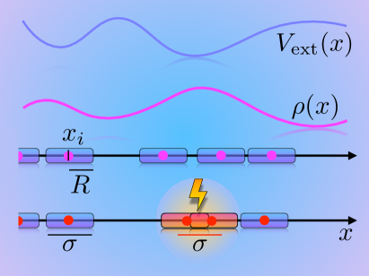
Figure 1: Illustration of hard rods in one spatial dimension that are exposed to a position-dependent external potential $V_{\rm ext}(x)$. In response to the external influence a spatially inhomogeneous density profile $\rho(x)$ emerges in equilibrium at temperature $T$ and chemical potential $\mu$. The particles with position coordinates $x_{i}$ and particle index $i=1,\ldots,N$ have radius $R$ and diameter $\sigma=2R$. A configuration is forbidden (bottom row) if any two particles overlap, i.e., if their mutual distance is smaller than the particle diameter $\sigma$.

In recent work, de las Heras et al. delasheras2023perspective and Sammüller et al. sammueller2023neural have put forward machine learning strategies that operate on the one-body level of correlation functions. Here we address in detail the neural functional theory sammueller2023neural for inhomogeneous fluids in equilibrium. We argue that this approach constitutes a neural network-based theory, where multiple different and mutually intimately related neural functionals form a genuine theoretical structure that permits investigation, testing, and to ultimately gain profound insight into the nature of the coupled many-body physics. Thereby the training is only required for a single neural network, from which then all further neural functionals are created in straightforward ways. The method allows for multi-scale application sammueller2023neural as is pertinent for many areas of soft matter schmid2022editorial ; baptista2021 ; gholami2021 . It is furthermore applicable to general interactions, as exemplified by successfully addressing a supercritical Lennard-Jones fluid sammueller2023neural , thus complementing analytical efforts to construct density functional approximations. Such work was based, e.g., on hierarchical integral equations yagi2021 ; yagi2022 , on functional renormalization group methods iso2019densityRenormalization ; yokota2021 ; kawana2023 , and on fundamental measure theory schmidt1999sfmt ; schmidt2000sfmtMix ; schmidt2000sfmtStructure .

Here we use the one-dimensional hard core model to illustrate the key concepts of the neural functional theory, as the required sampling can be performed easily and Percus’ functional provides an analytical structure that we can relate to the neural theory. The Percus functional is one of the very few general classical free energy density functionals that is analytically known for a continuum model (see e.g. also Refs. percus1982 ; buschle2000 ) and this fact provides further motivation for our study. A hands-on tutorial that demonstrates the key concepts of constructing a neural direct correlation functional, generating the required data from Monte Carlo simulations, testing against a numerical implementation of the Percus functional, and working with automatic differentiation is available online sammueller2023neuralTutorial .

The paper is structured into individual subsections, as described in the following; each subsection is self-contained to a significant degree such that Readers are welcome to select the description of those topics that match their own interests and individual backgrounds. An overview of key concepts of the one-body neural functional approach is given in Sec. I.1. This hybrid method draws on classical density functional concepts, as summarized in Sec. I.2. Functional differentiation and integration methods are described in Sec. I.3.

Readers who are primarily interested in the use of machine learning may want to skip the above material and rather start with Sec. II.1, where we describe how to construct and train the neural correlation functional on the basis of many-body simulation data. We concentrate on the specific model of one-dimensional hard core particles and complement and contrast the neural functional by the known exact analytical results for this model, as described in Sec. II.2. Model applications for predicting inhomogeneous systems based on neural density functional theory are described in Sec. II.3.

Several methods of neural functional calculus are described in Sec. III. Manipulating the neural correlation functional by functional integration and automatic functional differentiation is described in Secs. III.1 and III.2, respectively. The application of Noether sum rules as a standalone means for quality control of the neural network is presented in Sec. III.3. Functional integral sum rules are shown in Sec. III.4. A brief overview of key concepts of neural functional representations in nonequilibrium are presented in Sec. IV. We give conclusions in Sec. V.

I.1 Neural functional concepts

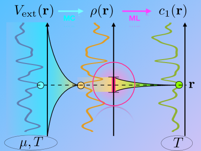
Figure 2: Illustration of the relevant functional maps of the neural functional theory. The external potential $V_{\rm ext}({\mathbf{r}})$ generates a one-body density profile $\rho({\mathbf{r}})$ that is associated with a one-body direct correlation function $c_{1}({\mathbf{r}})$. At given temperature $T$, chemical potential $\mu$, and for a specific form of the external potential $V_{\rm ext}({\mathbf{r}})$, Monte Carlo simulations provide data for the corresponding density profile $\rho({\mathbf{r}})$ and for the direct correlation function $c_{1}({\mathbf{r}})$. Machine learning is used to represent the functional map $\rho\to c_{1}$ via a deep neural network. The functional dependence of $c_{1}({\mathbf{r}})$ on the density profile is of much shorter spatial range as compared to the training data obtained from $V_{\rm ext}\to\rho$.

The neural functional framework sammueller2023neural rests on a combination of simulation, density functional theory, and machine learning. Data that characterizes the underlying many-body system is generated via grand canonical Monte Carlo simulations of well-defined, but random external conditions. Based on these results the one-body direct correlation functional is constructed as a neural network that accepts as an input the relevant local section of the density profile. This method allows for very efficient data handling as only short-ranged correlations contribute; Fig. 2 depicts an illustration.

The neural one-body direct correlation functional $c_{1}({\mathbf{r}},[\rho])$ forms the mother network for the subsequent functional calculus. Automatically differentiating the mother network with respect to its density input yields the two-body direct correlation functional $c_{2}({\mathbf{r}},{\mathbf{r}}^{\prime},[\rho])$ as a daughter functional. Two-body direct correlations are central in liquid state theory hansen2013 and they are here represented by a standalone numerical object that is created via straightforward application of automatic differentiation. This workflow is very different and arguabaly much simpler in practice than the standard technique of carrying out the functional differentiation analytically and then implementing the resulting expression(s) via numerical code.

Differentiating the daughter network yields a granddaughter network, which represents the three-body direct correlation functional $c_{3}({\mathbf{r}},{\mathbf{r}}^{\prime},{\mathbf{r}}^{\prime\prime},[\rho])$. Again this is an independent and standalone numerical computing object. Very little is known about three-body direct correlations, with e.g. Rosenfeld’s early investigation for hard spheres rosenfeld1989 and the freezing studies by Likos and Ashcroft likos1992 ; likos1993 being notable exceptions. The neural functional method sammueller2023neural offers arguably unprecedented detailed access.

Tracing the genealogy in the reverse direction requires functional integration, which is a general and standard technique in functional calculus. In the present case again a quasi-standalone numerical object can be built based on mere network evaluation and standard numerical integration, both of which are fast operations. In this way functionally integrating the mother one-body direct correlation functional creates as the grandmother the excess free energy functional $F_{\rm exc}[\rho]$. This mathematical object is the ultimate generating functional in classical density functional theory for all $n$-body direct correlation functions evans1979 ; hansen2013 ; schmidt2022rmp . We give more details about the interrelationships within the family of functionals below in Sec. I.3.

When applied to the three-dimensional hard sphere fluid and restricted to planar geometry, such that the density distribution is inhomogeneous only along a single spatial direction, the neural functional theory outperforms the best available hard sphere density functional (the formidable White Bear Mk. II fundamental measure theory roth2010 ) in generic inhomogeneous situations. For spatially homogeneous fluids the neural functional even surpasses the “very accurate equation of state” hansen2013 by Carnahan and Starling santos2020review , despite the fact that no explicit information about any bulk fluid properties was used during training.

Formulating reliable strategies of how to test machine-learning predictions constitutes in general a complex yet very important task, not least in the light of ongoing and projected increased use of artificial intelligence in science huang2023review . The neural functional theory offers a wealth of concrete self-consistency checks besides the standard benchmarking techniques. Commonly and following best practice in machine learning, benchmarking is performed by dividing the reference data, as here obtained from many-body simulations, into training, validation and test data. The simulations in the test data set have not been used during training and hence can serve to assess the performance of the trained network. In our present model application, we can perform testing directly with respect to the exact Percus theory.

Assessing extrapolation capabilities beyond the underlying data set requires the availability of further reference data. In Ref. sammueller2023neural this is provided by comparing (favourably) against a highly accurate bulk equation of state kolafa2004 as well as comparing against free energy reference results obtained from simulation-based thermodynamic integration of inhomogeneous systems.

However, due to its computational efficiency the neural approach allows to make predictions for system sizes that outscale significantly the dimensions of the original simulation box. Ref. sammueller2023neural describes systems of micron-sized colloids confined between parallel walls with macroscopic separation distance. The density profile is resolved over a system size of 1 mm with nanometric precision on a numerical grid with 10 nm spacing. Such “simulation beyond the box” is both powerful in terms of multiscale description of soft matter schmid2022editorial ; baptista2021 ; gholami2021 , but is also serves as template for the more general situation of using artificial intelligence methods far outside their original training realm.

In order to provide quality control, the neural functional theory hence allows to carry out a second type of test. This is less generic than the above benchmarking but it can nevertheless provide inspiration for machine learning in wider contexts. In the present case, the specific statistical mechanical nature of the underlying equilibrium many-body system implies far-reaching mathematical structure, as it lies at the very heart of Statistical Mechanics. Specifically, it is the significant body of equilibrium sum rules that provide formally exact interrelations between different types of correlation functions. These sum rules hold universally, i.e., independent of the specific inhomogeneous situation that is under consideration and they hence constitute formally exact relationships between functionals.

As the neural functional theory expresses direct correlation functions using neural network methods, the sum rules directly translate to identities that connect the different neural functionals and their integrated and differentiated relatives with each other. Crucially, these connections have both different mathematical form, as well as different physical meaning, as compared to the bare genealogy provided by the automatic functional differentiation and functional integration. Without overstretching the analogy, one could view the sum rules as genetic testing the entire family for absence of inheritable disease.

While the body of statistical mechanical sum rules is both significant and diverse baus1984 ; evans1990 ; henderson1992 ; upton1998 , here we rely on the recent Noether invariance theory hermann2021noether ; hermann2022topicalReview ; hermann2022variance ; tschopp2022forceDFT ; sammueller2022forceDFT ; hermann2022quantum ; sammueller2023whatIsLiquid ; robitschko2023any ; hermann2023whatIsLiquid as a systematic means to create both known and new functional identities from the thermal invariance of the underlying statistical mechanics hermann2021noether ; hermann2022topicalReview . In particular from invariance against local shifting one obtains sum rules that connect different generations of direct correlation functionals with each other in both locally-resolved and global form. We present exemplary cases below in Sec. III.3. Generic sum rules that emerge from the mere inverse relationship of functional integration and functional differentation are presented in Sec. III.4.

I.2 Introduction to classical density functional theory

We give a compact account of some key concepts of classical density functional theory; for more details see Refs. evans1979 ; evans1992 ; evans2016 ; hansen2013 ; schmidt2022rmp . Readers who are primarily interested in machine learning of neural functionals can skip this and the next subsection and directly proceed to Sec. II.

In a statistical mechanical description of a many-body system the local density acts as a generic order parameter that measures the probability of finding a particle at a specific location. The formal definition of the one-body density distribution as a statistical average is:

$$\rho({\mathbf{r}}) =\Big{\langle}{\sum_{i}\delta({\mathbf{r}}-{\mathbf{r}}_{i})}\Big{\rangle},$$ (1)

where the sum over $i$ runs over all $N$ particles, ${\mathbf{r}}_{i}$ is the position coordinate of particle $i=1,\ldots,N$, and $\delta(\cdot)$ indicates the Dirac distribution, here in three dimensions. The angles indicate a thermal average over microstates, which can e.g. be efficiently carried out in Monte Carlo simulations.

For completeness, we give a formal description of the equilibrium average based on the grand ensemble, where it is defined as $\langle\cdot\rangle={\rm Tr}\,\cdot{\rm e}^{-\beta(H-\mu N)}/\Xi$. Here the inverse temperature is $\beta=1/(k_{B}T)$, with the Boltzmann constant $k_{B}$ and absolute temperature $T$, the Hamiltonian $H$, chemical potential $\mu$ and grand partition sum $\Xi$. The classical trace is defined as ${\rm Tr}\,\cdot=\sum_{N=0}^{\infty}(h^{3N}N!)^{-1}\int d{\mathbf{r}}^{N}\int d{\bf p}^{N}\cdot$, where $h$ denotes the Planck constant and $\int d{\mathbf{r}}^{N}\int d{\bf p}^{N}$ is a shorthand for the high-dimensional phase space integral over all particle positions and momenta. Pedagogical introductions can be found in standard textbooks hansen2013 and an introductory compact account together with a description of the force point of view is provided in Ref. hermann2022topicalReview .

The Hamiltonian has the following standard form:

$$H=\sum_{i}\frac{{\bf p}_{i}^{2}}{2m}+u({\mathbf{r}}^{N})+\sum_{i}V_{\rm ext}({\mathbf{r}}_{i}),$$ (2)

where ${\bf p}_{i}$ is the momentum of particle $i$, the interparticle interaction potential $u({\mathbf{r}}^{N})$ depends on all position coordinates ${\mathbf{r}}^{N}={\mathbf{r}}_{1},\ldots,{\mathbf{r}}_{N}$, and $V_{\rm ext}({\mathbf{r}})$ is an external potential energy function that depends on position ${\mathbf{r}}$. Hence the sum in Eq. (2) comprises kinetic, interparticle, and external energy contributions. For the common case of particles interacting via a pair potential $\phi(r)$ that only depends on the interparticle distance $r$, the interparticle energy reduces to $u({\mathbf{r}}^{N})=\sum_{ij(\neq)}\phi(|{\mathbf{r}}_{i}-{\mathbf{r}}_{j}|)/2$ where the double sum runs only over distinct particle pairs $ij$ with $i\neq j$ and the factor $1/2$ corrects for double counting.

For the ideal gas the interparticle interactions vanish, $u({\mathbf{r}}^{N})\equiv 0$, and the density profile is given by the generalized barometric law hansen2013 :

$$\rho_{\rm id}({\mathbf{r}})={\rm e}^{-\beta(V_{\rm ext}({\mathbf{r}})-\mu)}/\Lambda^{d},$$ (3)

where $\Lambda$ denotes the thermal de Broglie wavelength, which in the present classical case can be set $\Lambda=\sigma$, with $\sigma$ denoting the particle size; for simplicity of notation here we use $\Lambda=1$; we have indicated the spatial dimensionality by $d$.

Taking the logarithm of Eq. (3) and collecting all terms on the left hand side gives the following ideal gas chemical potential balance:

$$\ln\rho_{\rm id}({\mathbf{r}})+\beta V_{\rm ext}({\mathbf{r}})-\beta\mu =0.$$ (4)

For a mutually interacting system, where $u({\mathbf{r}}^{N})\neq 0$, Eq. (4) will not be true when replacing the ideal density profile $\rho_{\rm id}({\mathbf{r}})$ by the true density profile $\rho({\mathbf{r}})$ as formally given by Eq. (1). Rather the sum of the three terms on the left hand side of Eq. (4) will not vanish, but yield a nontrivial contribution:

$$\ln\rho({\mathbf{r}})+\beta V_{\rm ext}({\mathbf{r}})-\beta\mu =c_{1}({\mathbf{r}}),$$ (5)

where the one-body direct correlation function $c_{1}({\mathbf{r}})$ is in general nonzero and arises due to the presence of interparticle interactions in the system. (For hard core systems $c_{1}({\mathbf{r}})$ typically features negative values.)

The machine learning strategy described below in Sec. II.1 is based on this pragmatic access to data for $c_{1}({\mathbf{r}})$, as obtained by direct simulation of $\rho({\mathbf{r}})$ on the basis of explicitly carrying out the average in Eq. (1) for given form of $V_{\rm ext}({\mathbf{r}})$ and prescribed values of the thermodynamic parameters $\mu$ and $T$. As the one-body direct correlation function is central in the neural functional theory, we combine Eqs. (4) and (5), which yields the following equivalent form for the one-body direct correlation function,

$$c_{1}({\mathbf{r}})=\ln\Big{(}\frac{\rho({\mathbf{r}})}{\rho_{\rm id}({\mathbf{r}})}\Big{)},$$ (6)

where $\rho_{\rm id}({\mathbf{r}})$ is given by Eq. (4) with $\Lambda=1$. Equation (6) has the direct interpretation of $c_{1}({\mathbf{r}})$ as the logarithm of the ratio of the actual density profile and the density profile of the ideal gas under identical conditions, as given by the external potential and thermodynamic statepoint.

In alternative terminology hansen2013 one defines the intrinsic chemical potential as $\mu_{\rm int}({\mathbf{r}})=\mu-V_{\rm ext}({\mathbf{r}})$. The intrinsic chemical potential and the one-body direct correlation function are related trivially to each other via $\mu_{\rm int}({\mathbf{r}})=k_{B}T[\ln\rho({\mathbf{r}})-c_{1}({\mathbf{r}})]$ as is obtained straightforwardly by re-arranging Eq. (5).

The practical, computational, and conceptual advantage of density functional theory lies in avoiding the explicit occurrence of the high-dimensional phase space integral that underlies thermal averages; we recall the definition of the density profile (1) as such an expectation value. Instead, and without any principal loss of information, one works with functional dependencies. Rather than mere point-wise dependencies, such as between the functions $\rho({\mathbf{r}})$, $V_{\rm ext}({\mathbf{r}})$, and $c_{1}({\mathbf{r}})$ that hold at each point ${\mathbf{r}}$, see Eq. (5), a functional dependence is on the entirety of a function and it has in general a nonlocal and nonlinear structure.

Density functional theory is specifically based on the fact hohenberg1964 ; mermin1965 ; evans1979 that for a given type of fluid, as characterized by its interparticle interaction potential $u({\mathbf{r}}^{N})$, and known thermodynamic parameters $\mu$ and $T$, the form of density profile $\rho({\mathbf{r}})$ is sufficient to determine the entirety of the external potential $V_{\rm ext}({\mathbf{r}})$. Hence a unique functional map exists hohenberg1964 ; mermin1965 ; evans1979 :

$$\rho\to V_{\rm ext}.$$ (7)

Here we omit the position arguments on both sides to reflect in the notation that the functional map relates the entirety of the density profile to the entirety of the external potential.

Applying Eq. (7) to the external potential, as it occurs in Eq. (5), implies that the left hand side is determined from knowledge of the density profile alone, in principle without any need for a priori knowledge of the form of $V_{\rm ext}({\mathbf{r}})$. Via the identity Eq. (5) we can conclude the existence of the map:

$$\rho\to c_{1},$$ (8)

where the entirety of the density profile determines the entirety of the direct correlation function. As a consequence the one-body direct correlation function actually is a density functional, $c_{1}({\mathbf{r}},[\rho])$, where the brackets indicate the functional dependence, i.e. on the entirety of the argument function, here $\rho({\mathbf{r}})$. We will discuss below more explicitly that the dependence is effectively short-ranged for the case of short-ranged interparticle interaction potentials and that this can be exploited to great effect in the neural network methodology.

I.3 Density functional derivatives and integrals

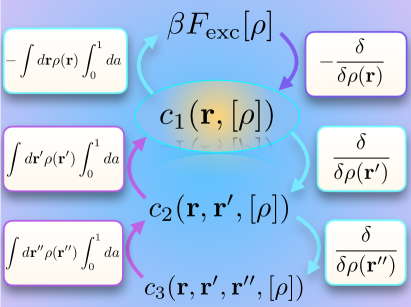
Figure 3: Illustration of four different generations of density functionals. Shown are the excess free energy functional $F_{\rm exc}[\rho]$ and the one-, two-, and three-body direct correlation functionals. Upward arrows indicate the relationship via functional integration $\int d{\mathbf{r}}\rho({\mathbf{r}})\int_{0}^{1}da$ with the integrand being evaluated at the scaled density $a\rho({\mathbf{r}})$. Downward arrows indicate functional differentiation $\delta/\delta\rho({\mathbf{r}})$. The neural functional theory is based on training $c_{1}({\mathbf{r}},[\rho])$ as the generating mother functional. Implementing the arrowed operations only requires high-level code. The resulting neural networks, as well as functionals derived from analytical expressions, are highly performant.

While we have emphasized above the role of the one-body direct correlation functional $c_{1}({\mathbf{r}},[\rho])$, primarily due to $c_{1}({\mathbf{r}})$ being directly measurable via Eq. (6), one typically rather starts with a parent functional, the excess free energy functional $F_{\rm exc}[\rho]$, in standard accounts of classical density functional theory. The relationship of $F_{\rm exc}[\rho]$ and $c_{1}({\mathbf{r}},[\rho])$ is established via functional calculus. Functional differentiation, see Ref. schmidt2022rmp for a practitioner’s account, yields additional position dependence and we use the notation $\delta/\delta\rho({\mathbf{r}})$ to denote the functional derivative with respect to the function $\rho({\mathbf{r}})$. Functional integration is the inverse operation. We give a brief description of the functional relationships in the following. An overview is illustrated in Fig. 3 and we will return for a broader account below in Sec. III.

The method of automatic differentiation baydin2018autodiff is an integral part of the new computing paradigm of differentiable programming chollet2017 . Automatic differentiation is based on a powerful set of techniques and it differs from both symbolic differentiation, as facilitated by computer algebra systems, and from numerical differentiation via finite difference, as is computational bread and butter. As shown in the tutorial sammueller2023neuralTutorial only high-level code is required to invoke automatic differentiation, and both neural and analytical functionals can be differentiated with little effort. As the derivative (of the functional) is with respect to its entire input data, the method constitutes a representation of a genuine functional derivative.

We give an overview. In the present context the functional calculus that relates the one-body direct correlations to the parent excess free energy functional is given by the following functional integration and functional differentiation relations:

$$\beta F_{\rm exc}[\rho] =-\int d{\mathbf{r}}\rho({\mathbf{r}})\int_{0}^{1}dac_{1}({\mathbf{r}},[\rho_{a}]),$$ (9)

$$c_{1}({\mathbf{r}},[\rho]) =-\frac{\delta\beta F_{\rm exc}[\rho]}{\delta\rho({\mathbf{r}})}.$$ (10)

In Eq. (9) we have parameterized the general formal integral $\int D[\rho]$ by using $\rho_{a}({\mathbf{r}})$ as a scaled version of the density profile, with a simple linear relationship $\rho_{a}({\mathbf{r}})=a\rho({\mathbf{r}})$. Hence the parameter value $a=0$ corresponds to vanishing density and $a=1$ reproduces the target density profile, as it occurs in the argument of $\beta F_{\rm exc}[\rho]$ on the left hand side of Eq. (9). We emphasize that the integral over $a$ in Eq. (9) is a simple one-dimensional integral over the coupling parameter $a$. The consistency between Eqs. (9) and (10) is demonstrated below in Sec. III.4.

The perhaps seemingly very formal functional calculus acquires new and pressing relevance in light of the neural functional concepts of Ref. sammueller2023neural , which allows to work explicitly with both functional derivatives and functional integrals, which can be evaluated efficiently via the corresponding standalone neural functionals.

In light of these benefits it is fortunate that the functional differentiation-integration structure extends recursively to higher orders of correlation functions. The next level beyond Eqs. (9) and (10) involves the two-body direct correlation functional $c_{2}({\mathbf{r}},{\mathbf{r}}^{\prime},[\rho])$ and the integration and differentiation structure is as follows:

$$c_{1}({\mathbf{r}},[\rho]) =\int d{\mathbf{r}}^{\prime}\rho({\mathbf{r}}^{\prime})\int_{0}^{1}dac_{2}({\mathbf{r}},{\mathbf{r}}^{\prime},[\rho_{a}]),$$ (11)

$$c_{2}({\mathbf{r}},{\mathbf{r}}^{\prime},[\rho]) =\frac{\delta c_{1}({\mathbf{r}},[\rho])}{\delta\rho({\mathbf{r}}^{\prime})},$$ (12)

and we refer to Refs. hansen2013 ; schmidt2022rmp ; brader2013noz ; brader2014noz for background.

We can chain the functional derivatives together by inserting $c_{1}({\mathbf{r}},[\rho])$ as given by Eq. (10) into the definition (12) of $c_{2}({\mathbf{r}},{\mathbf{r}}^{\prime},[\rho])$. In parallel, we can also chain the functional integrals in Eqs. (9) and (11). These procedures yield the following second order functional integration and differentiation relationships:

$$\beta F_{\rm exc}[\rho] =-\int d{\mathbf{r}}\rho({\mathbf{r}})\int d{\mathbf{r}}^{\prime}\rho({\mathbf{r}}^{\prime})$$

$$\qquad\times\int_{0}^{1}da\int_{0}^{a}da^{\prime}c_{2}({\mathbf{r}},{\mathbf{r}}^{\prime},[\rho_{a^{\prime}}]),$$ (13)

$$c_{2}({\mathbf{r}},{\mathbf{r}}^{\prime},[\rho]) =-\frac{\delta^{2}\beta F_{\rm exc}[\rho]}{\delta\rho({\mathbf{r}})\delta\rho({\mathbf{r}}^{\prime})},$$ (14)

where the scaled density profile in Eq. (13) is $\rho_{a^{\prime}}({\mathbf{r}})=a^{\prime}\rho({\mathbf{r}})$. The double parameter integral in Eq. (13) can be further simplified evans1992 , as described at the end of Sec. III.4. The generalization of Eq. (14) to the $n$-th functional derivative defines the $n$-body direct correlation functional, which remains functionally dependent on the density profile and which possesses spatial dependence on $n$ position arguments. Although increasing $n$ yields objects that become very rapidly out of any practical reach, the neural functional concept provides much fuel for making progress. While we do not cover $c_{3}({\mathbf{r}},{\mathbf{r}}^{\prime},{\mathbf{r}}^{\prime\prime},[\rho])$ here, Sammüller et al. have demonstrated its general accessiblity and physical validity for bulk fluids in Ref. sammueller2023neural .

We have so far focused on the properties of the intrinsic excess free energy functional $F_{\rm exc}[\rho]$ and its density functional derivatives. This is natural as classically $F_{\rm exc}[\rho]$ is the central object that contains the effects of the interparticle interactions and thus depends in a nontrivial way on its input density profile. The functional $F_{\rm exc}[\rho]$ is intrinsic in the sense that it is independent of external influence. We recall that we here work in the grand ensemble (see e.g. Refs. gonzalez1997 ; white2000 ; dwandaru2011 ; delasheras2014canonical for studies addressing the canonical ensemble of fixed particle number). Hence the appropriate thermodynamic potential is the grand canonical free energy or grand potential. This is required in order to determine $\rho({\mathbf{r}})$.

When expressed as a density functional the grand potential consists of the following sum of ideal, excess, external, and chemical potential contributions:

$$\Omega[\rho] =F_{\rm id}[\rho]+F_{\rm exc}[\rho]+\int d{\mathbf{r}}\rho({\mathbf{r}})[V_{\rm ext}({\mathbf{r}})-\mu].$$ (15)

The form of the ideal gas free energy functional is explicitly known as $F_{\rm id}[\rho]=k_{B}T\int d{\mathbf{r}}\rho({\mathbf{r}})[\ln\rho({\mathbf{r}})-1]$ and the third term in Eq. (15) contains the effects of the external potential $V_{\rm ext}({\mathbf{r}})$ and of the particle bath at chemical potential $\mu$.

The variational principle of classical density functional theory mermin1965 ; evans1979 ; dwandaru2011 ascertains that

$$\frac{\delta\Omega[\rho]}{\delta\rho({\mathbf{r}})}\Big{|}_{\rho=\rho_{0}} =0\quad{\rm(min)},$$ (16)

$$\Omega[\rho_{0}] =\Omega_{0}.$$ (17)

Equations (16) and (17) imply that the grand potential becomes minimal at $\rho_{0}({\mathbf{r}})$, which is the real, physically realized density profile and $\Omega_{0}$ is the equilibrium value of the grand potential. Recall that based on the many-body picture we have $\Omega_{0}=-k_{B}T\ln\Xi$ with the grand ensemble partition sum $\Xi={\rm Tr}\,{\rm e}^{-\beta(H-\mu N)}$. We have used the subscript 0 to denote equilibrium but we drop this elsewhere in our presentation to simplify notation.

Inserting Eq. (15) into Eq. (16) and using the explicit form of the ideal free energy functional together with the definition Eq. (10) of $c_{1}({\mathbf{r}},[\rho])$ leads to Eq. (5) with the one-body direct correlations expressed as a density functional, as anticipated in Sec. I.2. Exponentiating and regrouping the terms then yields the following popular form of the Euler-Lagrange equation:

$$\rho({\mathbf{r}})=\exp\Big{(}-\beta V_{\rm ext}({\mathbf{r}})+\beta\mu+c_{1}({\mathbf{r}},[\rho])\Big{)}.$$ (18)

Equation (18) is a self-consistency relation that can be solved efficiently for the equilibrium density profile $\rho({\mathbf{r}})$ via iterative methods, as detailed below in Sec. II.3. A prerequisite is that $c_{1}({\mathbf{r}},[\rho])$ is known, usually as an approximation that is obtained from an approximate excess free energy functional $F_{\rm exc}[\rho]$ via functionally differentiating according to Eq. (10). Having obtained a numerical solution of Eq. (18) for the density profile, this can then be inserted into the grand potential functional (15) to obtain full thermodynamic information via Eq. (17), which by construction is consistent with the density profile.

We demonstrate in the following how this classical functional background can be put to formidable use via hybridization with simulation-based machine learning. As our aim is pedagogical, we choose the one-dimensional hard core system as a concrete example to demonstrate the general methodology sammueller2023neural . We complement the neural functional structure with a description of Percus’ analytical solution, which then allows for mirroring of the neural theory.

II Neural functional theory

Jerry Percus famously wrote in the abstract of his 1976 statistical mechanics landmark paper percus1976 : “The external field required to produce a given density pattern is obtained explicitly for a classical fluid of hard rods. All direct correlation functions are shown to be of finite range in all pairs of variables.” Here we relate his achievement to the neural functional theory, which allows to reproduce numerically a variety of properties of the exact solution. We emphasize that the neural functional theory remains generic in its applicability to further model fluids; see the Supplementary Information of Ref. sammueller2023neural for the successful treatment of the supercritical Lennard-Jones fluid in three dimensions. We refer the Reader to the provided online resources sammueller2023neuralTutorial for a programming tutorial on the concrete application of the following concepts. Figure 4 shows a schematic of the workflow that is inherent in the neural functional concept, as described in the following.

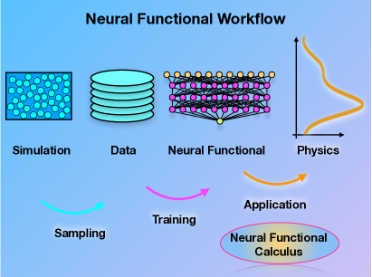
Figure 4: Schematic of the workflow of the neural functional theory. Many-body simulations under randomized conditions are used to sample statistically averaged and spatially resolved data that characterize the inhomogeneous response of the considered system. A neural network is then trained to represent the direct correlation functional, which is subsequently applied numerically and via neural functional methods to investigate the physics of the system in the desired target situations.

II.1 Training the neural correlation functional

The classical fluid of hard rods that Percus considers has one-dimensional position coordinates $x_{i}$, with particle index $i=1,\ldots,N$ and a pairwise interparticle interaction potential $\phi(x)$ which is infinite if the distance $x$ between the two particles is smaller than their diameter, $x<\sigma$, and it vanishes otherwise. The system is exposed to an external potential $V_{\rm ext}(x)$, which is a function of position $x$ across the system, and this in general creates an inhomogeneous “density pattern” $\rho(x)$.

We adjust the definition (1) of the density distribution to the present one-dimensional case:

$$\rho(x)=\Big{\langle}{\sum_{i}\delta(x-x_{i})}\Big{\rangle},$$ (19)

where $\delta(\cdot)$ here indicates the Dirac distribution in one dimension and the brackets indicate a grand canonical thermal average. Due to the hard core nature of the model, the statistical weight of each “allowed” microstate is particularly simple and given by $\exp[-\beta\sum_{i}V_{\rm ext}(x_{i})+\beta\mu N]/\Xi$, where $\Xi$ is a normalizing factor. Allowed microstates are those for which all distinct particle pairs $ij$ are spaced far enough apart, $|x_{i}-x_{j}|\geq\sigma$. If already a single overlap occurs, then the microstate is “forbidden” as the interparticle potential becomes formally infinite, which then creates vanishing statistical weight; we recall the illustration in Fig. 1.

Despite the apparent simplicity of the many-body probability distribution, the Statistical Mechanics of the hard rod model is nontrivial. The particles interact nonlocally over the lengthscale $\sigma$ and the external potential has no restrictions on its shape or on the lengthscale(s) of variation. Hence features such as jumps and positive infinities that represent hard walls are allowed. In bulk, $V_{\rm ext}(x)=0$, and the solution is straightforward tonks1936 ; hansen2013 . The general case is however highly nontrivial, which makes Percus’ above quoted opening a very remarkable one. We present more details of his work further below, after first laying out the general machine learning strategy of Ref. sammueller2023neural . This neural functional method is neither restricted to hard cores nor to one-dimensional systems, but addressing this case here is useful to highlight the salient features of the approach.

We aim for explicitly sampling the microstates of the system according to their probability distribution via particle-based simulations. This can be implemented efficiently, and for the present introductory purposes in also an intuitively accessible way, via grand canonical Monte Carlo (GCMC) sampling. Excellent accounts of this method are given in Refs. frenkel2023book ; hansen2013 ; wilding2001 ; brukhno2021dlmonte . Briefly, a Markov chain of microstates is constructed, where based on a given configuration, a trial step is proposed, which is accepted with a probability given by the Metropolis function $\min[1,\exp(-\beta\Delta E)]$, where $\Delta E$ is the energy difference between the original and the trial state.

Three trial moves are used in the simplest yet powerful scheme: i) Selecting one particle $i$ randomly and displacing it uniformly within a given maximal cutoff distance. If the displacement creates overlap, then the trial move is discarded. If otherwise there is no overlap in the new configuration, the energy difference is due to only the external potential, $\Delta E=V_{\rm ext}(x_{i})-V_{\rm ext}(x_{i}^{\prime})$, where the prime denotes the trial position of particle $i$. ii) A new particle $j$ is inserted at a random position $x_{j}$ with energy change that accounts for both the external potential and the chemical equilibrium with the particle bath and hence $\Delta E=V_{\rm ext}(x_{j}^{\prime})-\mu$. iii) Correspondingly, a randomly selected particle $i$ is removed from the system. The acceptance of the removal happens again with a probability given by the Metropolis function with energy difference $\Delta E=-V_{\rm ext}(x_{i})+\mu$.

Despite its conceptual simplicity GCMC is a very powerful method for the investigation of complex effects frenkel2023book ; wilding2001 ; brukhno2021dlmonte and significant extensions exist both in the form of histogram techniques wilding2001 ; brukhno2021dlmonte and the tailoring of more complex and collective trial moves. Investigating a typical physical problem, as specified by the interparticle interactions $u({\mathbf{r}}^{N})$ and the type of considered external influence, such as walls as represented by a model form of $V_{\rm ext}({\mathbf{r}})$, requires e.g. scanning of the thermodynamic parameters and acquiring good enough statistics at each statepoint. Our ultimate goal (Sec. II.3) is to perform this tasks with significant gain in efficiency via the neural theory; we re-iterate the availability via Ref. sammueller2023neuralTutorial of hands-on code examples for the present hard rod model.

We base the training on the following rewriting and adaption of the chemical potential balance Eq. (5) to the one-dimensional system:

$$c_{1}(x) =\ln\rho(x)+\beta V_{\rm ext}(x)-\beta\mu.$$ (20)

All quantities on the right hand side are either prescribed a priori or are accessible via the GCMC simulations: Specifically, the density profile $\rho(x)$ is obtained by filling a position-resolved histogram according to the encountered microstates as specified by its particle coordinates $x_{i}$. We recall the formal definition (19) of $\rho(x)$ via the Dirac distribution, which in practice is discretized such that sufficient finite spatial resolution, say $0.01\sigma$, is obtained. This “counting” method is arguably the most intuitive one to obtain data for the density profile. As an aside, there is a number of force-sampling techniques that can improve the statistical variance significantly borgis2013 ; delasheras2018forceSampling ; rotenberg2020 ; robitschko2023any and that also can serve to gauge the quality of sampling of the equilibrium ensemble robitschko2023any .

While the issues of Monte Carlo sampling efficiency and quality assessment of thermal averages can be pertinent in higher dimensions and in physically more complex situations, the simplicity of the present one-dimensional hard core model makes counting according to Eq. (19) an appropriate choice to obtain data for $\rho(x)$. Then adding up the three contributions on the right hand side of Eq. (20) yields results for $c_{1}(x)$. We proceed at this data-generation stage somewhat heretically and ignore at first the central role that $c_{1}(x)$ plays for the physics of inhomogeneous systems.

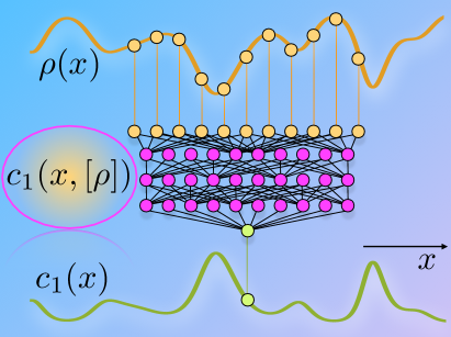
Figure 5: Illustration of the neural one-body direct correlation functional $c_{1}(x,[\rho])$ represented by a fully connected neural network with three hidden layers. The topology maps a small finite window of the density profile $\rho(x)$ to the local value of the direct correlation function $c_{1}(x)$.

In contrast to the typical deterministic setup for investigating a specific physical situation described above, training the neural network proceeds on the basis of randomized situations rather than with the ultimate application in mind; we recall the illustration of the neural functional workflow shown in Fig. 4. The motivation for using this strategy comes from the goal of capturing via the machine learning the intrinsic direct correlations of the many-body system that then transcend the specific inhomogeneous situations that were under consideration during training. Figure 5 depicts an illustration of the neural network topology of the trained central neural network $c_{1}(x,[\rho])$ and its relation to the physical input and output quantities, i.e., to $\rho(x)$ and $c_{1}(x)$.

We hence perform a sequence of simulation runs, where each run has an input value $\beta\mu^{(k)}$ and an input functional shape $\beta V_{\rm ext}^{(k)}(x)$, both of which are generated randomly. Specifically, we combine sinusoidal functions with periodicities that are commensurate with the box length $L$, linear discontinuous segments, and hard walls in the creation of $V_{\rm ext}^{(k)}(x)$; see Refs. sammueller2023neural ; sammueller2023neuralTutorial for further details. The superscript $k$ enumerates the different GCMC simulation runs and in practice we perform 512 of these. The result is a set of corresponding density profiles $\rho^{(k)}(x)$. We then use Eq. (20) to obtain for each run the one-body direct correlation profiles from simply adding up: $c_{1}^{(k)}(x)=\ln\rho^{(k)}(x)+\beta V_{\rm ext}^{(k)}(x)-\beta\mu^{(k)}$. As a result of the simulation protocol we have generated a bare data set $\{\beta\mu^{(k)},\beta V_{\rm ext}^{(k)}(x)$, $\rho^{(k)}(x)$, $c_{1}^{(k)}(x)\}$ for all positions $x$ and for all different runs $k$. As a practical detail, this requires to exclude regions where $\rho(x)=0$ and $V_{\rm ext}(x)=\infty$.

In order to address our declared goal to learn a functional dependence of $c_{1}(x)$, we have to carve out a nontrivial dependence relationship and hence restrict the data input. Motivated by the physics, one might see the scaled chemical potential $\beta\mu^{(k)}$ and the scaled external potential $\beta V_{\rm ext}^{(k)}(x)$ to be the true mechanical origin of the shape of the direct correlation function $c_{1}^{(k)}(x)$. However, the insights provided by density functional theory hint at the fact that this is not the best possible choice of functional relationship to consider.

We recap that the GCMC simulations yield data according to:

$$\big{\{}V_{\rm ext}^{(k)}(x^{\prime})-\mu^{(k)}\big{\}}_{0}^{L} \;\longrightarrow\;\big{\{}\rho^{(k)}(x)\big{\}}_{0}^{L},$$ (21)

where the curly brackets indicate all function values inside of the system box, with ranges $0\leq x^{\prime}\leq L$ and $0\leq x\leq L$; the arrow indicates an input-output relationship. Applying Eq. (20) to the entire data set also allows to have the direct correlation function as an output according to:

$$\big{\{}V_{\rm ext}^{(k)}(x^{\prime})-\mu^{(k)}\big{\}}_{0}^{L} \;\longrightarrow\;\big{\{}c_{1}^{(k)}(x)\big{\}}_{0}^{L}.$$ (22)

If one were to mimic the simulations directly by the neural network one would be tempted to base the training directly upon Eq. (22). In less clearcut machine-learning situations than considered here, it can be a standard strategy to attempt to represent the causal relationship, which governs the complex mathematical or real-world system under consideration, by a surrogate artificial intelligence model. The present functional formulation of Statistical Mechanics hints at potential caveats, such as the necessity of dealing with the full input and output data sets (parameter ranges of $x$ and $x^{\prime}$) across the entire system. Furthermore the specific physics of the mutually interacting rods appears to play no role.

The density functional-inspired training (Sec. I.2) proceeds very differently. We here take a pragmatic stance and attempt to create via training a neural representation of the dependence of $c_{1}(x)$ on $\rho(x)$ alone. This leads to a surrogate model $c_{1}(x,[\rho])$ based on the following mapping

$$\big{\{}\rho^{(k)}(x^{\prime})\big{\}}_{x-x_{c}}^{x+x_{c}}\;\longrightarrow\;c_{1}^{(k)}(x),$$ (23)

where the input on the left hand side consists of function values $\rho^{(k)}(x^{\prime})$ that lie inside the density window centered at $x$, i.e., only the values $x^{\prime}$ that lie within a narrow interval $x-x_{c}\leq x^{\prime}\leq x+x_{c}$. Here $x_{c}$ is a cutoff parameter that for short-ranged interparticle potentials is of the order of the particle size. For the present one-dimensional hard core system we set $x_{c}=\sigma$. Instead of having to output an entire function, as would be the case when attempting to learn via Eq. (22), here the output is merely the single value of the direct correlation function at the center of the density window. We recall that this target value is obtained from the simulation data via Eq. (20) such that $c_{1}^{(k)}(x)=\ln\rho^{(k)}(x)+\beta V_{\rm ext}^{(k)}(x)-\beta\mu^{(k)}$ for each run $k$. A simple GCMC code is provided online sammueller2023neuralTutorial , along with a pre-generated simulation data set and a pre-trained neural functional.

We choose the loss function to be the mean squared error of the neural network output compared to the simulation reference value for $c_{1}(x)$, as obtained via Eq. (20). As a further metric to gauge the training progress, we make use of the mean absolute error of reference and output. Both choices are standard chollet2017 . The quadratic loss is convenient as it is analytical and hence the machine-learning gradient-based methods directly apply. The mean absolute error is nonanlytical due to the modulus involved, but it is a useful supporting quantity that has a very direct interpretation.

After training the mean absolute error was of the order of $\sim 0.013$, which implies that the neural network prediction deviates on average by this value from the simulation data. Although the simulation data carries some statistical noise, its effect is comparatively smaller, when taking the numerical solution of the Percus theory (detailed below) as the reference.

Our training data consists of 512 simulation runs using a simulation box size of $L=10\sigma$. Each of the simulation runs requires only about three minutes runtime on a single CPU core of a standard desktop machine.

We use a standard fully-connected artificial neural network with three hidden layers that respectively possess 128, 64 and 32 nodes. We use 201 input nodes to represent the density profile in a finite window of size $1\sigma$ and spatial bin size $0.01\sigma$, where we recall that $\sigma$ is the particle size. To accommodate the local functional mapping, we reshape the training data into input density windows and corresponding output values of $c_{1}(x)$, where we also apply twofold data augmentation by exploiting mirror symmetry of the simulation results. Excluding regions where $V_{\rm ext}(x)=\infty$ and hence where Eq. (20) is not defined, this results in $\sim 10^{6}$ input-output pairs.

From the above description and without considering the background in density functional theory it is not evident that the training will be successful and minimize the loss satisfactorily to yield a trained network $c_{1}(x,[\rho])$. From a mathematical point of view, this raises the questions whether a corresponding object $c_{1}(x,[\rho])$ indeed exist and whether it is unique. And if so, is its structure simple enough that it can be written down explicitly?

II.2 Percus’ exact direct correlation functional

Due to Percus singular achievement percus1976 the one-body direct correlation functional $c_{1}(x,[\rho])$ for interacting hard rods in one spatial dimension is known analytically and this has triggered much subsequent progress, see e.g. Refs. robledo1981 ; vanderlick1989 ; bakhti2012 ; rosenfeld1988 ; rosenfeld1989 ; tarazona2000 ; roth2002WhiteBear ; roth2006WhiteBear ; roth2010 . The functional dependence on the density profile is nonlocal, as one would expect from the fact that the rods interact over the finite distance $\sigma$, and it is also nonlinear, as is consistent with the behaviour of a nontrivially interacting many-body system. The spatial dependence is characterized by convolution operations which, despite performing the task of coarse-graining, retain the full character of the microscopic interactions. The Percus functional provided motivation for developing so-called weighted-density approximations (WDA) hansen2013 , where the density profile is convolved with one or several weight functions that are then further processed to give the ultimate value of the density functional.

We here give the Percus direct correlation functional in Rosenfeld’s geometry-based fundamental measure representation, see Ref. percus2013 for a historical perspective. Instead of working with the particle diameter $\sigma$ as the fundamental lengthscale, Rosenfeld rather bases his description on the particle radius $R=\sigma/2$, which allows to find deep geometric meaning in Percus’ expressions and to also generalize to higher dimensions rosenfeld1988 ; rosenfeld1989 ; roth2010 .

The exact form rosenfeld1988 of the one-body direct correlation functional is analytically given as the following sum:

$$c_{1}(x,[\rho])= -\frac{\Phi_{0}(x-R)+\Phi_{0}(x+R)}{2}$$

$$-\int_{x-R}^{x+R}dx^{\prime}\Phi_{1}(x^{\prime}).$$ (24)

Here the two functions $\Phi_{0}(x)$ and $\Phi_{1}(x)$ each depend on two weighted densities $n_{0}(x)$ and $n_{1}(x)$ in the following form:

$$\Phi_{0}(x) =-\ln[1-n_{1}(x)],$$ (25)

$$\Phi_{1}(x) =\frac{n_{0}(x)}{1-n_{1}(x)}.$$ (26)

The weighted densities $n_{0}(x)$ and $n_{1}(x)$ are obtained from the bare density profile via spatial averaging:

$$n_{0}(x) =\frac{\rho(x-R)+\rho(x+R)}{2},$$ (27)

$$n_{1}(x) =\int_{x-R}^{x+R}dx^{\prime}\rho(x^{\prime}).$$ (28)

The discrete spatial averaging at positions $x\pm R$ in the weighted density (27) parallels that in the first term of Eq. (24). Similarly the position integral over the interval $[x-R,x+R]$ in Eq. (28) appears analogously in the second term of Eq. (24). These similarities are not by coincidence. The structure is rather inherited from the grandmother (excess free energy) functional, as is described in Sec. III.1.

Having the analytical solution (24)–(28) for $c_{1}(x,[\rho])$ allows for carrying out numerical evaluation and comparing against results from the neural functional $c_{1}(x,[\rho])$. The range of nonlocality, i.e., the distance across which information of the density profile enters the determination of $c_{1}(x,[\rho])$ via Eqs. (24)–(28) is strictly finite, as announced in Percus’ abstract percus1976 . As two averaging operations, each with range $\pm R$, are chained together, the composite procedure has a range of $\pm 2R=\pm\sigma$, inline with our truncation of the density profiles in the training data sets according to Eq. (23). A numerical implementation of Percus direct correlation functional is available online sammueller2023neuralTutorial .

II.3 Application inside and beyond the box

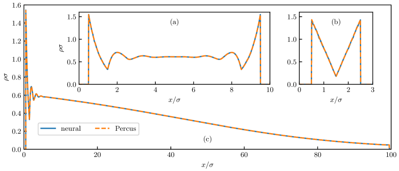
Figure 6: Representative density profiles that the inhomogeneous hard rod system exhibits under the influence of an external potential. The results are obtained from numerically solving Eq. (29) upon using either the neural direct correlation functional $c_{1}(x,[\rho])$ or Percus exact solution therof. The three cases comprise (a) two hards wall with separation distance $9\sigma$ and chemical potential $\beta\mu=2$, (b) two hard walls with much smaller separation distance $2\sigma$ and identical chemical potential $\beta\mu=2$, and (c) sedimentation-diffusion equilibrium under gravity with a locally varying chemical potential, $\beta\mu_{\rm loc}(x)=\beta\mu-\beta V_{\rm ext}(x)=2-0.05x/\sigma$; here the linearly varying contribution accounts for the influence of gravity on the system and confinement is provided by two widely spaced hard walls at $x=0.5\sigma$ und $x=99.5\sigma$. Note the crossover in panel (c) from the strongly oscillatory behaviour near the lower wall to a very smooth density decay, effectively following a local density approximation hansen2013 , upon increasing the scaled height $x/\sigma$.

Actually making the predictions for the hard rod model is now straightforward as we can resort to density functional theory and its standard use in application to physical problems. The arguably most common method for solving the Euler-Lagrange equation self-consistently is based on Eq. (18), which we re-express for the one-dimensional case considered:

$$\rho(x)=\exp\Big{(}-\beta V_{\rm ext}(x)+\beta\mu+c_{1}(x,[\rho])\Big{)}.$$ (29)

We recall that the range of nonlocality of $c_{1}(x,[\rho])$ is limited to only the particle size $\sigma$ and that we were able to extract the functional dependence from simulation data obtained by sampling in boxes of size $L$. Although the value of $L$ could in principle be imprinted in subtle finite size effects that $c_{1}(x,[\rho])$ has acquired, the size $L$ of the original simulation box has vanished and the application of the neural functional in Eq. (29) is fit for use to predict properties of much larger systems. As an example, Ref. sammueller2023neural demonstrates the scaling up by a factor of 100 from the original simulation box to the predicted system of three-dimensional hard spheres under gravity.

The numerical solution of Eq. (29) can be efficiently performed on the basis of Picard iteration where an initial guess of the density profile is inserted on the right hand side and the resulting left hand side is used to nudge the initial guess in the correct direction toward the self consistent solution. This is numerically fast and straightforward to implement, see the tutorial sammueller2023neuralTutorial . A common choice is to mix five percent of the new solution to the prior estimate.

As laid out above, we choose the one-dimensional hard core model due to both the availability of Percus’ functional and the computational ease of both numerical evaluation of the analytical expressions and of carrying out many-body simulations. On the downside, the model does not form a very credible platform for assessing the numerical efficiency gain of the neural theory, as in general one will be interested in more complex systems and more complex physical situations than addressed here. Nevertheless, to give a rough idea about the required computational workload, minimizing the neural density functional takes of the order of seconds on a GPU, while the GCMC simulation runtime is of the order of several minutes. Minimizing the analytical Percus functional is faster than using the neural network, due to the simple structure of Eqs. (24)–(28), which facilitates using very high-performance fast Fourier transforms.

We show three representative examples of density profiles for narrow to wide confinement between impenetrable walls in Fig. 6. In all cases the results from using the neural functional are numerically identical to those from the Percus functional on the scale of the plot. The profiles in narrow [Fig. 6(a)] and in moderately wide [Fig. 6(b)] pores show very dinstinct features with the strongly confined system in (a) having a striking V-shape, which arises from having at most two particles in the system, to the more generic damped oscillatory behaviour in the moderately wide pore (b). The main panel Fig. 6(c) shows the influence of a weak gravitational field, which creates a continuously varying density inhomogeneity across the entire system. The decay in local density occurs with a much larger length scale as compared to the particle packing effects that are localized near the lower wall.

The behaviour shown in Fig. 6(c) away from the walls is well-represented by a local density approximation hansen2013 (see e.g. Ref. jex2023 for recent mathematical work). The local density approximation can be a useful tool when investigating e.g. macroscopic ordering under gravity, where the occurring stacking sequences of different thermodynamic phases can be traced back to the phase diagram delasheras2015stacking ; eckert2021communPhys . In particular the effects on mixtures were rationalized by a range of techniques, from generalization of Archimedes’ principle piazza2008sedimentation ; piazza2012archimedes to analyzing stacking sequences delasheras2015stacking ; eckert2021communPhys . We stress that the present model applications constitute very significant extrapolations from the training data that we recall was obtained in a fixed box size $L=10\sigma$ and under the influence of randomized external and chemical potentials. Hence both the very confined system [Fig. 6(b)] and the large system [Fig. 6(c)] constitute significant extrapolations from the training data.

As a further potential application of the neural functional theory, the dynamical density functional theory evans1979 ; marconi1999 ; archer2004 is similarly easy to implement numerically as Eq. (29) and it is a currently popular choice to study time-dependent problems tevrugt2020review ; tevrugt2022perspective . We comment on the status of the approach delasheras2023perspective and how machine learning can help to overcome its limitations in Sec. IV below.

III Neural functional calculus

We have seen in Sec. II how a neural one-body direct correlation functional can be efficiently trained on the basis of a pool of pre-generated Monte Carlo simulation data that are obtained under randomized conditions. The specific way of organizing the simulation data into training sets mirrors the functional relationships given by classical density functional theory. We have then shown that the neural functional can efficiently be used to address physical problems, taking the one-dimensional hard rod system as a simple example of a mutually interacting many-body system.

We here proceed by exemplifying the depth of physical insight that can be explored by acknowledging the functional character of the trained neural correlation functional. Hence we lay out functional integration (Sec. III.1) and functional differentiation (Sec. III.2). We show sum rule construction via Noether invariance (Sec. III.3), via exchange symmetry (also Sec. III.3), and via functional integration (Sec. III.4). The presentation in each subsection is self-contained to a considerable degree and we illustrate the generality of the methods both by application to the neural functional as well as by revisiting the analytic Percus theory.

III.1 Functional integration of direct correlations

Having captured the essence of molecular packing effects, as they arise from the short-ranged hard core repulsion between the particles, via the neural functional $c_{1}(x,[\rho])$, begs for speculation whether additional and as yet hidden physical structure can be revealed. We give two plausibility arguments why one should expect to be able to postprocess $c_{1}(x,[\rho])$ in a meaningful way to retrieve global information.

First, thermodynamics is based on the existence of very few and well-defined unique and global quantities, such as the entropy, the internal energy, and the free energy. Carrying out parametric derivatives, with powerful interrelations given by the Maxwell relations, enables one to obtain equations of state, susceptibilities and further measurable global quantities. Our neural direct correlation functional in contrast is a local object with finite range of nonlocality. So how does this relate to the global information?

The second argument is more formal. Suppose we prescribe the form of the density profile and then evaluate the neural functional $c_{1}(x,[\rho])$ at each position $x$. This procedure yields a numerical representation of the corresponding direct correlation function $c_{1}(x)$. In the practical numerical representation we have a set of discrete grid points that represent the function values at these spatial locations $x$. Hence the entire data set forms a numerical array or numerical vector, indexed by $x$. One can then ask whether this vector could potentially be the gradient of an overarching parent object?

The physical and the formal question can both be answered affirmatively due to the existence of the excess free energy density functional $F_{\rm exc}[\rho]$. Its practical route of access, based on functional integration along a continuous sequence of states (a “line”) in the space of density functions, is strikingly straightforward within the neural method. The core of the method is to evaluate $c_{1}(x,[\rho_{a}])$ as described above, but for a range of scaled versions of the prescribed density profile $\rho_{a}(x)$ and then integrating in position to obtain the excess free energy as a global value, see the functional integral given in Eq. (9).

Specifically, we define a scaled version of the density profile as $\rho_{a}(x)=a\rho(x)$, such that $a=0$ generates the empty state that has vanishing density profile, $\rho_{a=0}(x)=0$. On the other end $a=1$ yields the actual density profile of interest, $\rho_{a=1}(c)=\rho(x)$. The excess free energy functional is then obtained easily via functional integration according to

$$\beta F_{\rm exc}[\rho] =-\int dx\rho(x)\int_{0}^{1}dac_{1}(x,[\rho_{a}]).$$ (30)

The numerical evaluation requires evaluation of $c_{1}(x,[\rho_{a}])$ at all positions $x$ in the system and for a range of intermediate values $0\leq a\leq 1$ such that the parametric integral over $a$ can be accurately discretized.

Analytically carrying out the functional integral (30) on the basis of the analytical direct correlation functional $c_{1}(x,[\rho])$ as given by Eqs. (24)–(28) is feasible. The result robledo1981 , again expressed in the more illustrative Rosenfeld fundamental measure form, is given by:

$$\beta F_{\rm exc}[\rho] =\int dx\Phi(n_{0}(x),n_{1}(x)),$$ (31)

$$\Phi(n_{1}(x),n_{2}(x)) =-n_{0}(x)\ln[1-n_{1}(x)].$$ (32)

Here the integrand $\Phi(n_{0}(x),n_{1}(x))$ plays the role of a localized excess free energy density which depends on the weighted densities $n_{0}(x)$ and $n_{1}(x)$ as given via the spatial averaging procedures in Eqs. (27) and (28), respectively. Inserting Eq. (32) into Eq. (31) yields the hard rod excess free energy functional in the following more explicit form:

$$\beta F_{\rm exc}[\rho] =-\int dxn_{0}(x)\ln[1-n_{1}(x)].$$ (33)

Equation (33) is strikingly compact, given that it describes the essence of a system of mutually interacting hard cores exposed to an arbitrary external potential.

Although the result of the functional integral (30) has lost all position dependence, the specific form of the density profile $\rho(x)$ is deeply baked into the resulting output value of the functional via both the prefactor $\rho(x)$ in the integrand in Eq. (30) and the evaluation of the direct correlation functional at the specifically scaled form $\rho_{a}(x)$. In parallel with this mathematical structure, the explicit form (33) of the Percus functional clearly demonstrates that the resulting value will depend nontrivially on the shape of the input density profile.

Having demonstrated that $F_{\rm exc}[\rho]$ as a global quantity can be obtained from appropriate functional integration of a locally resolved correlation functional $c_{1}(x,[\rho])$ naturally leads to the question whether a reverse path exists that would mirror the inverse structure provided by integration and differentiation known from ordinary calculus.

The availability of a corresponding derivative structure for functionals is quite significant, as this by construction generates spatial dependence, as indicated by $\delta/\delta\rho(x)$; see e.g. Ref. schmidt2022rmp for details. We can hence retrieve, or generate, the direct correlation functional as the functional density derivative of the intrinsic excess free energy functional:

$$c_{1}(x,[\rho])=-\frac{\delta\beta F_{\rm exc}[\rho]}{\delta\rho(x)}.$$ (34)

While we turn to more general functional differentiation below, we here address again the analytical case, which is useful as it reveals the origin of the double appearance of the two spatial weighting processes in Eqs. (24)–(28). Rosenfeld rosenfeld1989 introduced two weight functions $w_{0}(x)$ and $w_{1}(x)$, which respectively describe the end points of a particle and its interior one-dimensional “volume”:

$$w_{0}(x) =\frac{\delta(x-R)+\delta(x+R)}{2},$$ (35)

$$w_{1}(x) =\Theta(R-|x|),$$ (36)

where $\Theta(x)$ indicates the Heaviside unit step function, i.e., $\Theta(x\geq 0)=1$ and 0 otherwise. The weighted densities $n_{0}(x)$ and $n_{1}(c)$, as given respectively by Eqs. (27) and (28), can then be represented via convolution of the respective weight function of type $\alpha=0,1$ with the density profile according to

$$n_{\alpha}(x) =\int dx^{\prime}w_{\alpha}(x-x^{\prime})\rho(x^{\prime}).$$ (37)

In more compact notation we can express Eq. (37) as $n_{\alpha}(x)=(w_{\alpha}\ast\rho)(x)$, where the asterisk denotes the spatial convolution. Then the direct correlation functional is given by

$$c_{1}(x,[\rho]) =-\sum_{\alpha=0,1}(w_{\alpha}\ast\Phi_{\alpha})(x),$$ (38)

which is an exact rewriting of the form given in Eq. (24). The coefficients $\Phi_{\alpha}$ are obtained as partial derivatives of the scaled free energy density (32) via $\Phi_{\alpha}=\partial\Phi/\partial n_{\alpha}$. This derivative structure reveals the mechanism for the generation of the explicit forms $\Phi_{0}(x)$ and $\Phi_{1}(x)$, as respectively given by Eqs. (25) and (26).

III.2 Functional differentiation of direct correlations

While the above described use of functional differentiation in an analytical setting might appear to be very formal and perhaps limited in its applicability, we emphasize that the concept is indeed very general. Given a prescribed functional of a function $\rho(x)$, the functional derivative $\delta/\delta\rho(x)$ simply gives the gradient of the functional with respect to a change in the input function at a specific location $x$.

By applying the functional derivative in the present one-dimensional context to a given functional form of $c_{1}(x,[\rho])$, one obtains the two-body direct correlation functional and we recall the generic expression (12) of the two-body direct correlation functional:

$$c_{2}(x,x^{\prime},[\rho]) =\frac{\delta c_{1}(x,[\rho])}{\delta\rho(x^{\prime})}.$$ (39)

Using the Percus version (38) of the one-body direct correlation functional and carrying out the functional derivative on the right hand side of Eq. (39) gives via an analytical calculation the following nonlocal result:

$$c_{2}(x,x^{\prime},[\rho]) =-\sum_{\alpha\alpha^{\prime}}\big{(}w_{\alpha}\ast\Phi_{\alpha\alpha^{\prime}}\ast w_{\alpha^{\prime}}\big{)}(x,x^{\prime}).$$ (40)

We make the double asterisk convolution structure more explicit below. The coefficient functions in Eq. (40) are obtained as second partial derivatives via $\Phi_{\alpha\alpha^{\prime}}=\partial^{2}\Phi/\partial n_{\alpha}\partial n_{\alpha^{\prime}}$. Explicitly, we have $\Phi_{00}(x)=0$ and the symmetry $\Phi_{01}(x)=\Phi_{10}(x)$. The remaining terms are given by

$$\Phi_{01}(x) =\frac{1}{1-n_{1}(x)},$$ (41)

$$\Phi_{11}(x) =\frac{n_{0}(x)}{[1-n_{1}(x)]^{2}}.$$ (42)

Inserting these results into Eq. (40) and making the convolutions explicit yields the following expression:

$$c_{2}(x,x^{\prime},[\rho]) =-2\int dx^{\prime\prime}\frac{w_{0}(x-x^{\prime\prime})w_{1}(x^{\prime}-x^{\prime\prime})}{1-n_{1}(x^{\prime\prime})}$$

$$\quad-\int dx^{\prime\prime}\frac{w_{1}(x-x^{\prime\prime})n_{0}(x^{\prime\prime})w_{1}(x^{\prime}-x^{\prime\prime})}{[1-n_{1}(x^{\prime\prime})]^{2}}.$$ (43)

We recall the definitions (35) and (36) of the weight functions $w_{0}(x)$ and $w_{1}(x)$. The convolution structure couples two weight functions together and each of them has a range of $R$. Hence indeed the two-body direct correlations are of finite range $2R=\sigma$ in the position difference $x-x^{\prime}$ percus1976 .

While the above results for the Percus theory have been derived by pen-and-paper symbolic calculations, the neural functional is not amenable to such conventional techniques. Fortunately, the framework of automatic differentiation baydin2018autodiff provides a powerful alternative to both symbolic and numerical differentiation methods, and it is a natural choice to consider in the context of machine learning chollet2017 . Via the implementation of either modified algebra or of computational graphs, automatic differentiation facilitates to obtain derivatives directly in the form of executable code, and crucially there is no need of any manual intervention. Automatic differentiation thereby is free of the numerical artifacts that are typical of finite difference schemes. The method is applicable in broad contexts, which we illustrate in the online tutorial sammueller2023neuralTutorial by computing the Percus result for $c_{2}(x,x^{\prime})$ via automatic differentiation of Eq. (38) rather than by manual implementation of Eq. (43).

For completeness, we can recover the one-body direct correlation functional by functional integration. We reproduce Eq. (11) for the present one-dimensional geometry:

$$c_{1}(x,[\rho]) =\int dx^{\prime}\rho(x^{\prime})\int_{0}^{1}dac_{2}(x,x^{\prime},[\rho_{a}]).$$ (44)

On the basis of the neural representations of the direct correlation functionals, this identity can be used to check for consistency and for correctness of the automatic differentiation.

III.3 Noether invariance and exchange symmetry

In its standard applications Noether’s theorem is used to relate symmetries of a dynamical physical system with associated conservation laws. Obtaining linear momentum conservation from a symmetry of the underlying action integral is a primary example, see e.g. Ref. hermann2022topicalReview for an introductory presentation. Besides such deterministic applications, the Noether theorem is currently seeing an increased use in a variety of statistical mechanical settings baez2013markov ; marvian2014quantum ; sasa2016 ; sasa2019 ; revzen1970 ; budkov2022 ; brandyshev2023 ; bravetti2023 .

The recent statistical Noether invariance theory hermann2021noether ; hermann2022topicalReview ; hermann2022variance ; hermann2022quantum ; tschopp2022forceDFT ; sammueller2022forceDFT ; sammueller2023whatIsLiquid ; robitschko2023any ; hermann2023whatIsLiquid is based on specific spatial displacement (“shifting”) and rotation operations. These transformations are carried out in three-dimensional physical space and their effect is traced back to underlying invariances on the high-dimensional phase space and its associated thermal and nonequilibrium ensembles.

The central statistical Noether invariance concept hermann2021noether ; hermann2022topicalReview was demonstrated in a range of studies, addressing the strength of force fluctuations via their variance hermann2022variance , the formulation of force-based classical density functional theory tschopp2022forceDFT ; sammueller2022forceDFT , and the force balance in quantum many-body systems hermann2022quantum . The invariance theory has led to the discovery of force-force and force-gradient two-body correlation functions. These correlators were shown to deliver profound insight into the microscopic spatial liquid structure beyond the pair correlation function for a broad range of model fluids sammueller2023whatIsLiquid ; hermann2023whatIsLiquid . Noether invariance is relevant for any thermal observable, as associated sum rules couple the given observable to forces via very recently identified hyperforce correlations robitschko2023any .

The statistical Noether sum rules are exact identities that can serve a variety of different purposes, ranging from theory building via combination with approximate closure relations, testing for sufficient sampling in simulation robitschko2023any , carrying out force sampling to improve statistical data quality and, last but not least, testing neural functionals delasheras2023perspective ; sammueller2023neural . Having the latter purpose in mind, here we describe a selection of these Noether identities.

As a fundamental property, the interparticle interaction potential only depends on the relative particle positions and not on the absolute particle coordinate values. Specifically, whether two particles overlap in the one-dimensional system is unaffected by displacing the entire microstate uniformly. This invariance against global translation leads to associated sum rules for direct correlation functions; we recall that the direct correlations arise solely from the interparticle interactions and hence they are not directly dependent on the external potential. We quote two members of an infinite hierarchy of identities, which is originally due to Lovett, Mou, Buff, and Wertheim lovett1976 ; wertheim1976 , see Eqs. (45) and (46) below. We group these together with a recent curvature sum rule (47) hermann2022variance . Ultimately the identities (45) and (46) express the vanishing of the global interparticle force, as obtained by summing over the interparticle forces on all particles. The three sum rules read as follows:

$$\int dx\rho(x)\nabla c_{1}(x,[\rho]) =0,$$ (45)

$$\int dx\rho(x)\int dx^{\prime}\rho(x^{\prime})\nabla c_{2}(x,x^{\prime},[\rho]) =0,$$ (46)

$$\int dx[\nabla\rho(x)]\int dx^{\prime}[\nabla^{\prime}\rho(x^{\prime})]c_{2}(x,x^{\prime},[\rho]) =$$

$$-\int dx\rho(x) \nabla\nabla c_{1}(x),$$ (47)

where in the one-dimensional system the gradient is a simple scalar position derivative, $\nabla=d/dx$. Briefly, Eq. (45) is obtained by noting that $F_{\rm exc}[\rho]=F_{\rm exc}[\rho_{\boldsymbol{\epsilon}}]$, where the displaced density profile is given by $\rho_{\boldsymbol{\epsilon}}({\mathbf{r}})=\rho({\mathbf{r}}+{\boldsymbol{\epsilon}})$ with displacement vector ${\boldsymbol{\epsilon}}$ (in three dimensional systems). Building the gradient with respect to ${\boldsymbol{\epsilon}}$ yields the result $0=\partial\beta F_{\rm exc}[\rho_{\boldsymbol{\epsilon}}]/\partial{\boldsymbol{\epsilon}}|_{{\boldsymbol{\epsilon}}=0}=\int d{\mathbf{r}}(\delta\beta F_{\rm exc}[\rho]/\delta\rho({\mathbf{r}}))\nabla\rho({\mathbf{r}})$, which gives Eq. (45) upon integration by parts, resorting to the one-dimensional geometry, and identifying the one-body direct correlation functional via Eq. (34); for more details of the derivation we refer the Reader to Refs. hermann2021noether ; hermann2022topicalReview . Equation (46) is then obtained as the density functional derivative of Eq. (45) and re-using Eq. (45) to simplify the result. Equation (47) is a curvature sum rule that follows from spatial Noether invariance at second order in the global shifting parameter ${\boldsymbol{\epsilon}}$ hermann2021noether .

Using a locally resolved shifting operation, where the displacement ${\boldsymbol{\epsilon}}({\mathbf{r}})$ is local and depends on the spatial position ${\mathbf{r}}$ and hence constitutes a vector field (in the case of a three-dimensional system), yields in one dimension the following position-resolved identity:

$$\nabla c_{1}(x,[\rho]) =\int dx^{\prime}c_{2}(x,x^{\prime},[\rho])\nabla^{\prime}\rho(x^{\prime}).$$ (48)

The left hand side has the direct interpretation of the mean interparticle force field, expressed in units of the thermal energy $k_{B}T$. This force both acts in equilibrium and it drives the adiabatic part of the time evolution in nonequilibrium schmidt2022rmp ; we describe some details of the nonequilibrium theory for time evolution in Sec. IV.

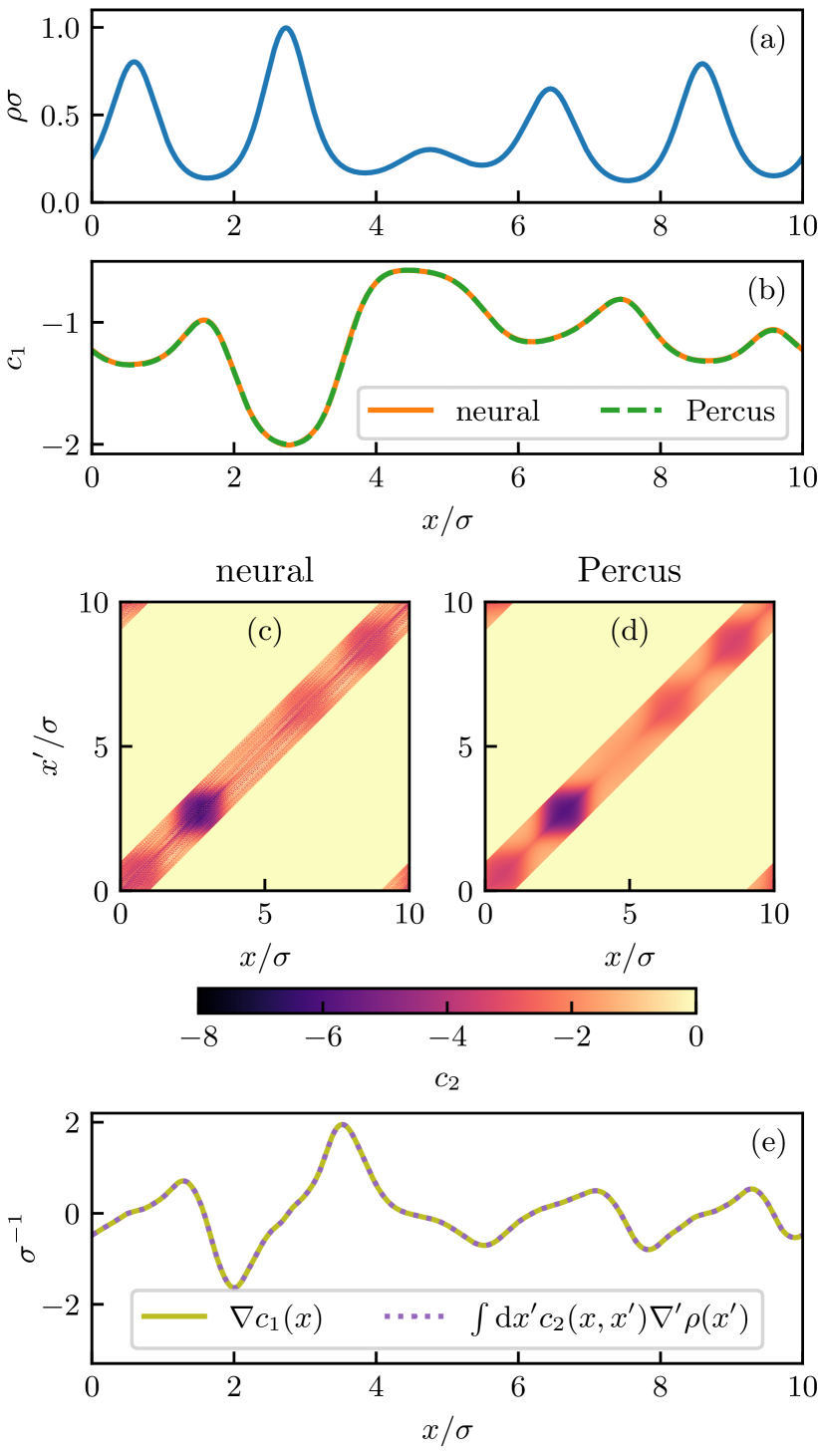
Figure 7: Numerical results for functional calculus and Noether invariance. The results are shown for an exemplary oscillatory density profile displayed in panel (a). Results for the neural prediction for $c_{1}(x)$ are compared to numerically evaluating Percus’ analytical direct correlation functional (24) in panel (b). The two-body direct correlation function $c_{2}(x,x^{\prime})$ as a function of $x/\sigma$ and $x^{\prime}/\sigma$, as obtained from automatic differentiation of the neural functional is shown in panel (c) and compared to the result from using Percus’ analytical expression (43) in panel (d). Using the neural functionals, the agreement of the left and right hand side of of the Noether force sum rule (48) is shown in panel (e). In all cases the neural functional and Percus theories give numerically identical results on the scale of the respective plot.

When inserting the relationship (34) of $c_{1}(x,[\rho])$ to the free energy functional $F_{\rm exc}[\rho]$ into the definition (39) of $c_{2}(x,x^{\prime},[\rho])$ we obtain

$$c_{2}(x,x^{\prime},[\rho]) =-\frac{\delta^{2}\beta F_{\rm exc}[\rho]}{\delta\rho(x)\delta\rho(x^{\prime})},$$ (49)

which is the one-dimensional version of the general relationship (14). As the order of the two functional derivatives is irrelevant we obtain the following exact symmetry with respect to the exchange of the two position arguments:

$$c_{2}(x,x^{\prime},[\rho]) =c_{2}(x^{\prime},x,[\rho]).$$ (50)

When applied to the neural functional, the exchange symmetry relationship (50) is highly nontrivial, as the density windows that enter the functionals on the left and on the right hand sides differ markedly from each other, as do the corresponding evaluation positions. That both displacement effects cancel each other and lead to the identity (50) is nontrivial and can serve both for testing the quality of the neural direct correlation functional and for demonstrating the existence of an overarching grandmother functional $F_{\rm exc}[\rho]$.

In order to illustrate the theoretical structure, we display numerical results in Fig. 7. We select a representative oscillatory density profile, as shown in Fig. 7(a), and take this as an input to evaluate the one-body direct correlation functional $c_{1}(x,[\rho])$. This procedure yields a specific form of the direct correlation function $c_{1}(x)$, displayed in Fig. 7(b), which belongs to the prescribed density profile $\rho(x)$. The spatial variations of $\rho(x)$ and $c_{1}(x)$ are roughly out-of-phase with each other. The nonlinear and nonlocal nature of the functional relationship $\rho\to c_{1}$ is however very apparent in the plot. The results from choosing the neural functional or Percus’ analytical one-body direct correlation functional agree with each other to excellent accuracy. The agreement is demonstrated in Fig. 7(b), where the two resulting direct correlation profiles are identical on the scale of the plot.

As laid out above above, the exchange symmetry (50) constitutes a rigorous test for the two-body direct correlation functional $c_{2}(x,x^{\prime},[\rho])$. Both the neural and the analytical functional pass with flying colours, see Figs. 7(c) and (d) respectively, where the symmetry of the respective “heatmap” graph against mirroring at the diagonal is strikingly visible.

As a representative case for the use of a Noether sum rule as a quantitative test for the accuracy of the neural functional methods, we show in Fig. 7(e) the numerical results of evaluating both sides of Eq. (48) for the same given density profile [shown in Fig. 7(a)]. We find that both sides of the equation agree with high numerical precision with each other.

III.4 Functional integral sum rules

We next address general identities that emerge from exploiting the inverse nature of functional differentiation and integration. For this, we recall the functional integral form (9) of $F_{\rm exc}[\rho]$ and the functional derivative form (10) of $c_{1}(\rho,[\rho])$, which both are central for the following derivations. That Eq. (9) is the inverse of Eq. (10) can be seen explicitly by functionally differentiating Eq. (9) as follows:

$$\frac{\delta\beta F_{\rm exc}[\rho]}{\delta\rho({\mathbf{r}})}=-\int d{\mathbf{r}}^{\prime}\int_{0}^{1}da\frac{\delta}{\delta\rho({\mathbf{r}})}\rho({\mathbf{r}}^{\prime})c_{1}({\mathbf{r}}^{\prime},[\rho_{a}]).$$ (51)

We have interchanged the order of integration and functional differentiation on the right hand side of Eq. (51) as these operations are independent of each other. The functional density derivative now acts on the product $\rho({\mathbf{r}}^{\prime})c_{1}({\mathbf{r}}^{\prime},[\rho_{a}])$ and we need to differentiate both factors according to the product rule. Differentiating the first factor gives the Dirac distribution, $\delta\rho({\mathbf{r}}^{\prime})/\delta\rho({\mathbf{r}})=\delta({\mathbf{r}}-{\mathbf{r}}^{\prime})$. Differentiating the second factor generates the two-body direct correlation functional according to Eq. (39) and hence $\delta c_{1}({\mathbf{r}}^{\prime},[\rho_{a}])/\delta\rho({\mathbf{r}})=ac_{2}({\mathbf{r}},{\mathbf{r}}^{\prime},[\rho_{a}])$, where multiplication by the scaling factor $a$ arises from the identity $\delta/\delta\rho({\mathbf{r}})=a\delta/\delta(a\rho({\mathbf{r}}))=a\delta/\delta\rho_{a}({\mathbf{r}})$.

We can hence reformulate Eq. (51) by rewriting the left hand side via Eq. (10) and expressing the right hand side by the two separate terms. Upon multiplication by $-1$ the result is the following functional integral identity:

$$c_{1}({\mathbf{r}},[\rho])= \int_{0}^{1}dac_{1}({\mathbf{r}},[\rho_{a}])$$

$$+\int d{\mathbf{r}}^{\prime}\rho({\mathbf{r}}^{\prime})\int_{0}^{1}daac_{2}({\mathbf{r}},{\mathbf{r}}^{\prime},[\rho_{a}]).$$ (52)

In the first term on the right hand side of Eq. (52) the position integral has cancelled out due to the presence of the Dirac function, which leaves over the position dependence on ${\mathbf{r}}$, as occurring in all other terms.

In order to prove Eq. (52) and hence to establish that indeed Eqs. (9) and (10) are inverse of each other, we integrate by parts in $a$ addressing the first integral on the right hand side of Eq. (52). This yields a sum of boundary terms and an integral: $c_{1}({\mathbf{r}},[\rho])-0-\int_{0}^{1}daa\partial c_{1}({\mathbf{r}},[\rho_{a}])/\partial a$. The derivative with respect to the parameter $a$ generates the second term in Eq. (52) up to the minus sign upon carrying out the parametric derivative via $\partial/\partial a=\int d{\mathbf{r}}^{\prime}\rho({\mathbf{r}}^{\prime})\delta/\delta\rho_{a}({\mathbf{r}}^{\prime})$ and identifying $c_{2}({\mathbf{r}},{\mathbf{r}}^{\prime},[\rho_{a}])=\delta c_{1}({\mathbf{r}},[\rho_{a}])/\delta\rho_{a}({\mathbf{r}}^{\prime})$. Hence the two integrals cancel each other. Only the upper boundary term $c_{1}({\mathbf{r}},[\rho])$ remains, which is the left hand side of Eq. (52), and hence completes the proof.

Despite this explicit derivation via functional calculus, as both $c_{1}({\mathbf{r}},[\rho])$ and $c_{2}({\mathbf{r}},{\mathbf{r}}^{\prime},[\rho])$ are directly available as neural functionals, the functional integral sum rule (52) provides yet again fresh possibility for carrying our consistency and accuracy checks.

Going through the analogous chain of arguments one generation younger leads to the following functional integral relationship between the two- and three-body direct correlation functionals:

$$c_{2}({\mathbf{r}},{\mathbf{r}}^{\prime},[\rho]) =\int_{0}^{1}dac_{2}({\mathbf{r}},{\mathbf{r}}^{\prime},[\rho_{a}])$$

$$\quad+\int d{\mathbf{r}}^{\prime\prime}\rho({\mathbf{r}}^{\prime\prime})\int_{0}^{1}daac_{3}({\mathbf{r}},{\mathbf{r}}^{\prime},{\mathbf{r}}^{\prime\prime},[\rho_{a}]).$$ (53)

The neural functional calculus allows to obtain $c_{3}({\mathbf{r}},{\mathbf{r}}^{\prime},{\mathbf{r}}^{\prime\prime},[\rho])$ via automatic generation of the Hessian of $c_{1}({\mathbf{r}},[\rho])$ sammueller2023neural , which elevates Eq. (53) beyond mere formal interest.

The structure of Eqs. (52) and (53) expresses a general functional relationship. When applied to the excess free energy functional itself the result is:

$$\beta F_{\rm exc}[\rho] =\int_{0}^{1}da\beta F_{\rm exc}[\rho_{a}]$$

$$\quad-\int d{\mathbf{r}}\rho({\mathbf{r}})\int_{0}^{1}daac_{1}({\mathbf{r}},[\rho_{a}]).$$ (54)

We furthermore demonstrate explicitly the relationship from daughter to grandmother via functional integration of the two-body correlation functional to obtain the excess free energy functional:

$$\beta F_{\rm exc}[\rho] =-\int d{\mathbf{r}}\rho({\mathbf{r}})\int d{\mathbf{r}}^{\prime}\rho({\mathbf{r}}^{\prime})$$

$$\qquad\times\int_{0}^{1}da\int_{0}^{a}da^{\prime}c_{2}({\mathbf{r}},{\mathbf{r}}^{\prime},[\rho_{a^{\prime}}]),$$ (55)

where again the scaled density profile is $\rho_{a^{\prime}}({\mathbf{r}})=a^{\prime}\rho({\mathbf{r}})$. That Eq. (55) holds can be seen by chaining together the two levels of functional integrals (9) and (44) and then simplifying the two nested parameter integrals. The double parametric integral in Eq. (55) can alternatively be written with fixed parametric boundaries as $\int_{0}^{1}daa\int_{0}^{1}da^{\prime}c_{2}({\mathbf{r}},{\mathbf{r}}^{\prime},[\rho_{aa^{\prime}}])$, where the twice scaled density profile is defined as $\rho_{aa^{\prime}}({\mathbf{r}})=aa^{\prime}\rho({\mathbf{r}})$.

Evans evans1992 goes further than Eq. (55) by using the identity $\int_{0}^{1}da\int_{0}^{a}da^{\prime}f(a^{\prime})=\int_{0}^{1}da(1-a)f(a)$, which is valid for any function $f(a)$, as can either by shown geometrically by considering the triangle-shaped integration domain in the two-dimensional $(a,a^{\prime})$-plane or, more formally, by integration by parts. The identity allows to express Eq. (55) in a form that requires to carry out only a single parametric integral:

$$\beta F_{\rm exc}[\rho] =-\int d{\mathbf{r}}\rho({\mathbf{r}})\int d{\mathbf{r}}^{\prime}\rho({\mathbf{r}}^{\prime})$$

$$\qquad\times\int_{0}^{1}da(1-a)c_{2}({\mathbf{r}},{\mathbf{r}}^{\prime},[\rho_{a}]).$$ (56)

Evans evans1992 also considers more general cases where the parameter $a$ linearly interpolates between a nontrivial initial density profile $\rho_{i}({\mathbf{r}})\neq 0$ and the target profile $\rho({\mathbf{r}})$ via $\rho_{a}({\mathbf{r}})=\rho_{i}({\mathbf{r}})+a[\rho({\mathbf{r}})-\rho_{i}({\mathbf{r}})]$. In our present description we have restricted ourselves to empty initial states, $\rho_{i}({\mathbf{r}})=0$, but the functional integration methodology is more general, see Ref. evans1992 .

Throughout we have notated the functional integrals via an outer position integral over ${\mathbf{r}}$ and an inner parametric integral over $a$. This structure allows to take the common factor $\rho({\mathbf{r}})$ out of the inner integral. Standard presentations often reverse the order of integration. Taking the functional integral over the one-body direct correlation functional as an example, both versions are identical:

$$\int d{\mathbf{r}}\rho({\mathbf{r}})\int_{0}^{1}dac_{1}({\mathbf{r}},[\rho_{a}]) =\int_{0}^{1}da\int d{\mathbf{r}}\rho({\mathbf{r}})c_{1}({\mathbf{r}},[\rho_{a}]).$$ (57)

Our (mild) preference for the order on the left hand side of Eq. (57) has two reasons. i) In a numerical scheme, where one discretizes on a grid of positions ${\mathbf{r}}$ and of values of $a$, the multiplication by $\rho({\mathbf{r}})$ is only required to be carried out once at each gridpoint ${\mathbf{r}}$, when using the left hand side, not also for every value of $a$ as on the right hand side. ii) Although the result of the inner integral, $\int_{0}^{1}dac_{1}({\mathbf{r}},[\rho_{a}])$, depends on the specific chosen parameterization $\rho_{a}({\mathbf{r}})$ and is hence not unique from the viewpoint of the entire functional, it nevertheless constitutes a well-defined localized function of ${\mathbf{r}}$.

IV Nonequilibrium dynamics

We have so far demonstrated that the equilibrium properties of correlated many-body systems can be investigated on a very deep level by using neural networks to represent the functional relationship that are inherent in the statistical physics. The required computational workload is thereby only quite moderate. The neural functionals that encapsulate the nontrivial information about correlations and about thermodynamics are lean, robust and they can be manipulated efficiently by the neural functional calculus outlined above.

These features of the neural theory naturally lead one to wonder about the potential applicability beyond equilibrium, i.e., to situations where the considered system is driven by external forces such that flow is generated. The recent nonequilibrium machine-learning method by de las Heras et al. delasheras2023perspective is based on the dynamical one-body force balance relationship for overdamped Brownian motion. The required dynamical functional dependencies are those given by power functional theory schmidt2022rmp . The power functional approach is formally exact and it goes beyond dynamical density functional theory evans1979 ; marconi1999 ; archer2004 ; chan2004 ; goddard2012prl ; goddard2021wellposedness in that it also captures nonequilibrium interparticle force contributions that exceed those generated by the free energy functional; see Refs. schmidt2022rmp ; schilling2022 ; tevrugt2020review ; tevrugt2022perspective for recent reviews. Such genuine nonequilibrium effects include viscous and structural nonequilibrium force fields schmidt2022rmp ; delasheras2018velocityGradient ; stuhlmueller2018prl ; delasheras2020fourForces , which for uniaxial compressional flow of a three-dimensional Lennard-Jones fluid were shown to be well-represented by a trained neural network delasheras2023perspective .

The neural nonequilibrium force fields were successfully compared against analytical power functional approximations, where simple and physically motivated semi-local dependence on both the local density and the local velocity was shown to capture correctly the essence of the forces that occur in the nonequilibrium situation. Together with the exact force balance equation, this allows to predict and to design nonequilibrium steady states delasheras2023perspective . The approach offers a systematic way to go beyond dynamical density functional theory and to address genuine nonequilibrium beyond a free energy description. We recall studies based on dynamical density functional theory that addressed non-equilibrium sedimentation of colloids royall2007dynamicSedimentation , the self-diffusion of particles in complex fluids bier2008prl , and the behaviour of the van Hove two-body dynamics of colloidal Brownian hard disks stopper2018dtpl and of hard spheres treffenstaedt2021dtpl ; treffenstaedt2022dtpl .

Several current statistical mechanical research threads are dedicated to the force point of view. This includes novel force-sampling techniques that significantly reduce the seemingly inherent statistical noise in many-body simulation results for key quantities, such as the density profile borgis2013 ; delasheras2018forceSampling ; rotenberg2020 ; renner2023torqueSampling . The statistical Noether invariance theory hermann2021noether ; hermann2022topicalReview ; hermann2022variance ; tschopp2022forceDFT ; sammueller2022forceDFT ; hermann2022quantum ; sammueller2023whatIsLiquid ; robitschko2023any ; hermann2023whatIsLiquid generates formal expressions for force correlation functions very naturally. Corresponding exact sum rules interrelate correlations that involve forces, force gradients, and more general observables in a hyperforce framework robitschko2023any . Force-based density functional approaches were put forward both quantum mechanically tokatly2005one ; tokatly2005two ; tokatly2007 ; tchenkoue2019 ; tarantino2021 and classically tschopp2022forceDFT ; sammueller2022forceDFT .

We have briefly touched on the concept of forces when discussing the direct correlation sum rule (48). Locally resolved force fields are central to power functional theory schmidt2022rmp ; schmidt2013pft ; schmidt2015qpft ; schmidt2018md for the description of the nonequilibrium dynamics of underlying many-body systems. The connection to the present framework is via the locally resolved interparticle force density ${\bf F}_{\rm int}({\mathbf{r}},t)$. When expressed in correlator form, this vector field is given as the following nonequilibrium average:

$${\bf F}_{\rm int}({\mathbf{r}},t) =-\Big{\langle}{\sum_{i}\delta({\mathbf{r}}-{\mathbf{r}}_{i})\nabla_{i}u({\mathbf{r}}^{N})}\Big{\rangle}.$$ (58)

The dependence on time $t$ arises as the average on the right hand side of Eq. (58), which is taken over the instantaneous nonequilibrium many-body probability distribution, as given by temporal evolution of the Smoluchowski equation for the case of overdamped dynamics. The interparticle force density ${\bf F}_{\rm int}({\mathbf{r}},t)$ can be split into a sum of an equilibrium-like “adiabatic” force density ${\bf F}_{\rm ad}({\mathbf{r}},t)$ and a genuine nonequilibrium “superadiabatic” contribution ${\bf F}_{\rm sup}({\mathbf{r}},t)$. Making the functional dependencies explicit, as they arise in power functional theory schmidt2022rmp , gives the following sum of two contributions:

$${\bf F}_{\rm int}({\mathbf{r}},t,[\rho,{\bf v}]) ={\bf F}_{\rm ad}({\mathbf{r}},t,[\rho])+{\bf F}_{\rm sup}({\mathbf{r}},t,[\rho,{\bf v}]).$$ (59)

Here the functional arguments are the density profile $\rho({\mathbf{r}},t)$ and the one-body velocity field ${\bf v}({\mathbf{r}},t)={\bf J}({\mathbf{r}},t)/\rho({\mathbf{r}},t)$, which are both microscopically resolved in space and in time. The numerator is the one-body current, which is given as an instantaneous nonequilibrium average via ${\bf J}({\mathbf{r}},t)=\langle\sum_{i}\delta({\mathbf{r}}-{\mathbf{r}}_{i}){\bf v}_{i}\rangle$, where ${\bf v}_{i}({\mathbf{r}}^{N},t)$ is the velocity of particle $i$ in the underlying many-body overdamped Brownian dynamics.

Reference delasheras2023perspective presents a demonstration of the validity of the functional dependence on $\rho({\mathbf{r}},t)$ and ${\bf v}({\mathbf{r}},t)$ via successful machine-learning of ${\bf F}_{\rm int}({\mathbf{r}},t,[\rho,{\bf v}])$ for inhomogeneous nonequilibrium steady states. The strategy for constructing the neural network is similar to that described here, but it is based on predicting the locally resolved nonequilibrium forces rather than the equilibrium one-body direct correlations. One important connection between equilibrium and nonequilibrium is given by the adiabatic construction schmidt2022rmp that relates ${\bf F}_{\rm ad}({\mathbf{r}},t,[\rho])$ in the nonequilibrium system to an instantaneous equilibrium system with identical density profile $\rho({\mathbf{r}},t)$. The adiabatic force field is then given as a density functional via the standard relationship

$${\bf F}_{\rm ad}({\mathbf{r}},t,[\rho])=k_{B}T\rho({\mathbf{r}},t)\nabla c_{1}({\mathbf{r}},[\rho]),$$ (60)

where the density argument of the one-body direct correlation functional $c_{1}({\mathbf{r}},[\rho])$ is the instantaneous density distribution $\rho({\mathbf{r}},t)$.

For overdamped Brownian dynamics with friction constant $\gamma$, the one-body current ${\bf J}({\mathbf{r}},t)$ appears in the force density balance, which is given by

$$\gamma{\bf J}({\mathbf{r}},t) =-k_{B}T\nabla\rho({\mathbf{r}},t)+{\bf F}_{\rm int}({\mathbf{r}},t)+\rho({\mathbf{r}},t){\bf f}_{\rm ext}({\mathbf{r}},t),$$ (61)

where ${\bf f}_{\rm ext}({\mathbf{r}},t)$ is an external force field that acts on the system, in general in a time- and position-dependent fashion. The prescription for the current is complemented by the microscopically resolved continuity equation, $\partial\rho({\mathbf{r}},t)/\partial t=-\nabla\cdot{\bf J}({\mathbf{r}},t)$. Upon neglecting the superadiabatic force density in Eq. (59) and hence only taking adiabatic forces into account, i.e. approximating ${\bf F}_{\rm int}({\mathbf{r}},t,[\rho,{\bf v}])\approx{\bf F}_{\rm ad}({\mathbf{r}},t,[\rho])$, one arrives at the dynamical density functional theory evans1979 ; marconi1999 ; archer2004 . Its inherent central approximation is hence to replace the nonequilibrium forces by effective equilibrium forces that are obtained from the free energy functional via the adiabatic construction schmidt2022rmp .

Returning to the one-dimensional geometry of the hard rod model, this leads to the following closed approximate equation of motion for the time-dependent density profile:

$$\frac{\partial\rho(x,t)}{\partial t}=$$

$$\quad D_{0}\nabla\Big{[}\nabla\rho(x,t)-\rho(x,t)\Big{(}\nabla c_{1}(x,[\rho])+\beta f_{\rm ext}(x,t)\Big{)}\Big{]}.$$ (62)

The derivative is simply $\nabla=\partial/\partial x$ in one dimension and the diffusion constant $D_{0}=k_{B}T/\gamma$ is the ratio of thermal energy and the friction constant. Equation (62) can be efficiently propagated in time with a simple forward Euler algorithm and the neural representation of $c_{1}(x,[\rho])$ can be used in lieu of an analytic approximation. However superadiabatic forces, i.e. force contributions that go beyond the adiabatic approximation of working with a free energy functional, are neglected. These include viscous and structural nonequilibrium contributions; we refer the Reader to Ref. schmidt2022rmp for background and to Ref. delasheras2023perspective for a recent perspective on the description of microscopic nonequilibrium dynamics of fluids in the light of machine learning on the basis of power functional theory.

V Conclusions and outlook

In conclusion we have given a detailed account of the recent neural functional theory sammueller2023neural for the structure and thermodynamics of spatially inhomogeneous classical many-body systems. The approach is based on input data obtained from Monte Carlo simulations that provide results for averaged density profiles. Thereby the training systems are exposed to the influence of randomized external potentials. Based on the functional relationships that are rigorously given by classical density functional theory, the training data is used to construct a neural network representation of the one-body direct correlation functional, which acts as a fundamental “mother” object in the neural functional theory.

From automatic functional differentiation of the one-body direct correlation functional follow daughter and granddaughter functionals that represent two- and three-body direct correlation functionals. Conversely, functional integration yields the neural excess free energy functional, which acts as the ultimate grandmother functional in the genealogy. We have shown that chaining together the functional differentiation and integration operations yields exact functional sum rules. Further exact identities are given by the statistical mechanical Noether invariance theory hermann2021noether ; hermann2022topicalReview ; hermann2022variance ; tschopp2022forceDFT ; sammueller2022forceDFT ; hermann2022quantum ; sammueller2023whatIsLiquid ; robitschko2023any ; hermann2023whatIsLiquid , by variety of fundamental liquid state techniques hansen2013 ; baus1984 ; evans1990 ; henderson1992 ; upton1998 and by functional calculus alone evans1979 ; evans1992 . We have described a selection of these sum rules in detail and have shown how their validity can be used to carry out consistency and accuracy checks for the different levels of mutually related neural density functionals.

We have here in particular focused on the one-dimensional hard rod systems for reasons of ease of data generation via simulations sammueller2023neuralTutorial , the availability of Percus’ exact functional percus1976 , the possibility of analytical manipulations to be carried out, and not least the fundamental character of this classical model tonks1936 . A beginner-friendly interactive code tutorial is provided online sammueller2023neuralTutorial , together with stand-alone documentation that describes the key strategies and the essence of the methods that constitute the neural functional theory sammueller2023neural . We have discussed prototypical applications for “simulation beyond the box”, where the neural functional is used for system sizes that outscale the dimension of the original training box that was used to generate the underlying Monte Carlo data sammueller2023neural . We have also given an overview of nonequilibrium methods and have emphasized the important role of the occurring force fields and their functional dependencies.

We recall that a detailed description of the setup of the paper is given before the start of Sec. I.1; the modular structure of the paper invites for selective reading. An overview of the relevant statistical mechanical concepts is given in Sec. I. The neural functional theory is described in detail in Sec. II and we have emphasized the important concept of local learning, as illustrated in Fig. 2, which facilitates very efficient network construction and training. The neural functional approach allows to explicitly carry out functional calculus as presented in Sec. III and it is relevant for nonequilibrium as described in Sec. IV. We once more highlight the availability of the online tutorial sammueller2023neuralTutorial , which covers all key aspects of our study and includes a practitioner’s account of automatic differentiation and differentiable programming.

The neural functional theory is a genuine hybrid method that draws with comparable weight from computer simulations, machine learning, and density functional theory. The compuational and conceptual complexities of the involved methods from each respective field are relatively low. Yet their combination offers a new and arguably unprecedented view of the statistical physics of many-body systems. We lay out in the following why the approach is interesting from the viewpoints of each of the three constituent approaches.

From the machine-learning perspective it seems unusual to have a large set of testable self-consistency conditions available. These conditions stem from statistical mechanical sum rules, as they follow e.g. from the Noether invariance theory, the functional integration-differentiation structure, and exchange symmetry. Taking the latter case as an example, that the automatic derivative of a neural network satisfies the exchange symmetry of its two (position) arguments is very remarkable, see the graphical demonstration of the diagonal symmetry in Fig. 7(c). This is a purely structural test for the quality of the network that does not require any independent reference data as a benchmark. All presented sum rules are of this type and they hence provide intrinsic constraints, either genuinely following from the underlying Statistical Mechanics or from mere functional calculus alone, which is the case for the functional integration-differentiation formalism outlined in Sec. III.4. Crucially, in our methodology the constraints are not enforced during training the network, as is done in methods of physics-informed machine learning in the classical density functional malpica-morales2023 and wider karniadakis2021 ; jung2023piml contexts.

From a computer simulation point of view the neural functional methods offer a new way of designing simulation work. Instead of direct simulation of the physical problem at hand, an intervening step of constructing the direct correlation functional is introduced. We have shown that the direct correlation functional can thereby be obtained explicitly and accurately. Rather than playing the role of a formal object, its availability as a trained neural network facilitates making fast and precise predictions in nontrivial situations. This application stage of the neural functional theory requires very little effort both in terms of the required numerical algorithmic structure and the computational workload; we recall the illustration of the neural functional workflow shown in Fig. 4.

From a density functional perspective the neural approach is arguably unprecedented in its degree of access to the excess free energy functional. We find it highly remarkable that so much of the seemingly very abstract functional relationships and formal concepts can be inspected and tested in computationally straightforward and highly efficient ways. The range of these methods includes automatic differentiation to generate direct correlation functions as well as performant functional integration routines. The neural functional framework offers the possibility to work numerically with exact functional identities with great ease. Hence the neural network technology relieves one from the task of constructing an approximate analytical functional and manipulating it on paper.

This leaves over the question of the status of analytical density functionals in the light of the neural network capabilities. We have here deliberately chosen the exact Percus functional for one-dimensional hard rods to demonstrate how much insight can be gleaned from the analytical manipulations; as a representative example see the nonlinear convolutional structure of Eqs. (24)–(28) along with the excellent numerical comparison against the neural functional as shown in Fig. 7(b). As the neural functional method is not restricted to the hard core system, one can expect that having an accurate neural functional for a given system can be of very significant help when attempting first-principles construction of analytical free energy functionals. After all we should make use of the tools that van der Waals did not have at his disposal!

In summary, in light of the progress reported in Refs. delasheras2023perspective ; sammueller2023neural and the present model investigation, we anticipate that a wealth of deep questions can be addressed from the viewpoint of the neural functional theory, including fundamental questions of phase coexistence binder2012 as well as the possible construction of fundamental measure functionals leithall2011 ; schmidt2011internalEnergy . While we here have restricted ourselves to hard core systems, the principal applicability of the neural functional theory for soft potentials was demonstrated in Ref. sammueller2023neural for (planar) inhomogeneities of the supercritical three-dimensional Lennard-Jones fluid. Going beyond planar geometry and addressing spatial inhomogeneity in two or three dimensions could benefit from the use of equivariant neural networks cohen2016 ; weiler2018 ; finzi2020 ; satorras2021 ; batzner2022 ; batzner2023 ; musaelian2023 , which possess the fundamental symmetry properties of Euclidean space.

For complex Hamiltonians the required amount of simulation work to provide training data might seem as a limitation. We are however optimistic that the subsequent efficient use of the direct correlation functionals in the form of neural networks can by far outweigh the training cost. Hence the application to complex models such as the monatomic Molinero-Moore water model molinero2009 ; coe2022water might not be out of reach. Furthermore it is inspiring to think that potential progress could be made in the treatment of dielectric cox2020pnas and long-ranged forces bui2024 .

As a final note, we re-emphasize the successful application of the neural method to nonequilibrium flow problems presented in Ref. delasheras2023perspective and it is certainly very inspiring to speculate whether this facilitates making progress concerning questions of slow dynamics in soft matter jung2023piml ; jung2023roadmap ; sammueller2023gel and beyond that HISML2023 .

- (1) J. D. van der Waals, Thermodynamische Theorie der Kapillarität unter Voraussetzung stetiger Dichteänderung (Thermodynamic theory of capillarity under the hypothesis of a continuous variation of density), Z. Phys. Chem. 13U, 657 (1894); English translation, J. S. Rowlinson, J. Stat. Phys. 20, 197 (1979).
- (2) J. S. Rowlinson and B. Widom, Molecular Theory of Capillarity (Dover, New York, 2002).
- (3) P. Hohenberg and W. Kohn, Inhomogeneous electron gas, Phys. Rev. 136, B864 (1964).
- (4) N. D. Mermin, Thermal properties of the inhomogeneous electron gas, Phys. Rev. 137, A1441 (1965).
- (5) R. Evans, The nature of the liquid-vapour interface and other topics in the statistical mechanics of non-uniform, classical fluids, Adv. Phys. 28, 143 (1979).
- (6) R. Evans, M. Oettel, R. Roth, and G. Kahl, New developments in classical density functional theory, J. Phys.: Condens. Matter 28, 240401 (2016).
- (7) R. Evans, Density functionals in the theory of nonuniform fluids, Chap. 3 in Fundamentals of Inhomogeneous Fluids, edited by D. Henderson (Dekker, New York, 1992).
- (8) J. P. Hansen and I. R. McDonald, Theory of Simple Liquids, 4th ed. (Academic Press, London, 2013).
- (9) M. Schmidt, Power functional theory for many-body dynamics, Rev. Mod. Phys. 94, 015007 (2022).
- (10) W. Kohn and L. J. Sham, Self-consistent equations including exchange and correlation effects, Phys. Rev. 140, A1133 (1965).
- (11) W. Kohn, Nobel Lecture: Electronic structure of matter–Wave functions and density functionals, Rev. Mod. Phys. 71, 1253 (1999).
- (12) R. Evans, D. Frenkel, and M. Dijkstra, From simple liquids to colloids and soft matter, Phys. Today 72, 38 (2019).
- (13) M. Levesque, R. Vuilleumier, and D. Borgis, Scalar fundamental measure theory for hard spheres in three dimensions: Application to hydrophobic solvation, J. Chem. Phys. 137, 034115 (2012).
- (14) R. Evans, M. C. Stewart, and N. B. Wilding, A unified description of hydrophilic and superhydrophobic surfaces in terms of the wetting and drying transitions of liquids, Proc. Natl. Acad. Sci. 116, 23901 (2019).
- (15) M. K. Coe, R. Evans, and N. B. Wilding, Density depletion and enhanced fluctuations in water near hydrophobic solutes: identifying the underlying physics, Phys. Rev. Lett. 128, 045501 (2022).
- (16) G. Jeanmairet, M. Levesque, and D. Borgis, Molecular density functional theory of water describing hydrophobicity at short and long length scales. J. Chem. Phys. 139, 154101 (2013).
- (17) D. Martin-Jimenez, E. Chacón, P. Tarazona, and R. Garcia, Atomically resolved three-dimensional structures of electrolyte aqueous solutions near a solid surface, Nat. Commun. 7, 12164 (2016).
- (18) J. Hernández-Muñoz, E. Chacón, and P. Tarazona, Density functional analysis of atomic force microscopy in a dense fluid, J. Chem. Phys. 151, 034701 (2019).
- (19) P. Cats, R. Evans, A. Härtel, and R. van Roij, Primitive model electrolytes in the near and far field: Decay lengths from DFT and simulations, J. Chem. Phys. 154, 124504 (2021).
- (20) M. Baus, Broken symmetry and invariance properties of classical fluids, Mol. Phys. 51, 211 (1984).
- (21) R. Evans and A. O. Parry, Liquids at interfaces: what can a theorist contribute? J. Phys.: Condens. Matter 2, SA15 (1990).
- (22) J. R. Henderson, Statistical mechanical sum rules, Chap. 2 in Fundamentals of Inhomogeneous Fluids, edited by D. Henderson (Dekker, New York, 1992).
- (23) P. J. Upton, Fluids against hard walls and surface critical behavior, Phys. Rev. Lett. 81, 2300 (1998).
- (24) P. S. Clegg, Characterising soft matter using machine learning, Soft Matter, 17, 3991 (2021).
- (25) M. Dijkstra and E. Luijten, From predictive modelling to machine learning and reverse engineering of colloidal self-assembly, Nature Materials 20, 762 (2021).
- (26) E. Boattini, M. Dijkstra, and L. Filion, Unsupervised learning for local structure detection in colloidal systems, J. Chem. Phys. 151, 154901 (2019).
- (27) G. Campos-Villalobos, E. Boattini, L. Filion, and M. Dijkstra, Machine learning many-body potentials for colloidal systems, J. Chem. Phys. 155, 174902 (2021).
- (28) G. Campos-Villalobos, G. Giunta, S. Marín-Aguilar, and M. Dijkstra, Machine-learning effective many-body potentials for anisotropic particles using orientation-dependent symmetry functions, J. Chem. Phys. 157, 024902 (2022).
- (29) F. A. Rodrigues, Machine learning in physics: a short guide, EPL 144, 22001 (2023).
- (30) J. Wu and M. Gu, Perfecting liquid-state theories with machine intelligence, J. Phys. Chem. Lett. 14, 10545 (2023).
- (31) T. Santos-Silva, P. I. C. Teixeira, C. Anquetil-Deck, and D. J. Cleaver, Neural-network approach to modeling liquid crystals in complex confinement, Phys. Rev. E 89, 053316 (2014).
- (32) S.-C. Lin and M. Oettel, A classical density functional from machine learning and a convolutional neural network, SciPost Phys. 6, 025 (2019).
- (33) S.-C. Lin, G. Martius, and M. Oettel, Analytical classical density functionals from an equation learning network, J. Chem. Phys. 152, 021102 (2020).
- (34) P. Cats, S. Kuipers, S. de Wind, R. van Damme, G. M. Coli, M. Dijkstra, and R. van Roij, Machine-learning free-energy functionals using density profiles from simulations, APL Mater. 9, 031109 (2021).
- (35) C. Qiao, X. Yu, X. Song, T. Zhao, X. Xu, S. Zhao, and K. E. Gubbins, Enhancing gas solubility in nanopores: a combined study using classical density functional theory and machine learning, Langmuir 36, 8527 (2020).
- (36) P. Yatsyshin, S. Kalliadasis, and A. B. Duncan, Physics-constrained Bayesian inference of state functions in classical density-functional theory, J. Chem. Phys. 156, 074105 (2022).
- (37) A. Malpica-Morales, P. Yatsyshin, M. A. Duran-Olivencia, and S. Kalliadasis, Physics-informed Bayesian inference of external potentials in classical density functional theory, J. Chem. Phys. 159, 104109 (2023).
- (38) X. Fang, M. Gu and J. Wu, Reliable emulation of complex functionals by active learning with error control, J. Chem. Phys. 157, 214109 (2022).
- (39) A. Simon, J. Weimar, G. Martius, and M. Oettel, Machine learning of a density functional for anisotropic patchy particles, J. Chem. Theory Comput. 20, 1062 (2024).
- (40) D. de las Heras, T. Zimmermann, F. Sammüller, S. Hermann, and M. Schmidt, Perspective: How to overcome dynamical density functional theory, J. Phys.: Condens. Matter 35, 271501 (2023). (Invited Perspective).
- (41) F. Sammüller, S. Hermann, D. de las Heras, and M. Schmidt, Neural functional theory for inhomogeneous fluids: Fundamentals and applications, Proc. Natl. Acad. Sci. 120, e2312484120 (2023).
- (42) F. Sammüller, Neural functional theory for inhomogeneous fluids – Tutorial; for online access see the URL: https://github.com/sfalmo/NeuralDFT-Tutorial .
- (43) R. Nagai, R. Akashi, S. Sasaki, and S. Tsuneyuki, Neural-network Kohn-Sham exchange-correlation potential and its out-of-training transferability, J. Chem. Phys. 148, 241737 (2018).
- (44) J. Schmidt, C. L. Benavides-Riveros, and M. A. L. Marques, Machine learning the physical nonlocal exchange-correlation functional of density-functional theory, J. Phys. Chem. Lett. 10, 6425 (2019).
- (45) Y. Zhou, J. Wu, S. Chen, and G. Chen, Toward the exact exchange-correlation potential: A three-dimensional convolutional neural network construct, J. Phys. Chem. Lett. 10, 7264 (2019).
- (46) R. Nagai, R. Akashi, and O. Sugino, Completing density functional theory by machine learning hidden messages from molecules, npj Comput. Mater. 6, 43 (2020).
- (47) L. Li, S. Hoyer, R. Pederson, R. Sun, E. D. Cubuk, P. Riley, and K. Burke, Kohn-Sham equations as regularizer: Building prior knowledge into machine-learned physics, Phys. Rev. Lett. 126, 036401 (2021).
- (48) H. Li, N. Zou, M. Ye, R. Xu, X. Gong, and W. Duan, Deep-learning density functional theory Hamiltonian for efficient ab initio electronic-structure calculation, Nat. Comput. Sci. 2, 367 (2022).
- (49) J. Gedeon, J. Schmidt, M. J. P. Hodgson, J. Wetherell, C. L. Benavides-Riveros, and M. A. L. Marques, Machine learning the derivative discontinuity of density-functional theory, Mach. Learn.: Sci. Technol. 3, 015011 (2022).
- (50) R. Pederson, B. Kalita, and K. Burke, Machine learning and density functional theory, Nat. Rev. Phys. 4, 357 (2022).
- (51) B. Huang, G. F. von Rudorff, O. A. von Lilienfeld, The central role of density functional theory in the AI age, Science 381, 170 (2023).
- (52) A. Santos, S. B. Yuste, and M. L. de Haro, Structural and thermodynamic properties of hard-sphere fluids, J. Chem. Phys. 153, 120901 (2020).
- (53) C. P. Royall, P. Charbonneau, M. Dijkstra, J. Russo, F. Smallenburg, T. Speck, C. Valeriani, Colloidal hard spheres: triumphs, challenges and mysteries, arXiv:2305.02452.
- (54) L. Tonks, The complete equation of state of one-, two- and three-dimensional gases of hard elastic spheres, Phys. Rev. 50, 955 (1936).
- (55) J. K. Percus, Equilibrium state of a classical fluid of hard rods in an external field, J. Stat. Phys. 15, 505 (1976).
- (56) A. Robledo and C. Varea, On the relationship between the density functional formalism and the potential distribution theory for nonuniform fluids, J. Stat. Phys. 26, 513 (1981).
- (57) T. K. Vanderlick, H. T. Davis and J. K. Percus The statistical mechanics of inhomogeneous hard rod mixtures, J. Chem. Phys. 91, 7136 (1989).
- (58) B. Bakhti, S. Schott, and P. Maass, Exact density functional for hard-rod mixtures derived from Markov chain approach, Phys. Rev. E 85, 042107 (2012).
- (59) J. K. Percus, A random walk to fundamental measure theory–A mini-review at a personal level, J. Stat. Phys. 150, 601 (2013).
- (60) Y. Rosenfeld, Scaled field particle theory of the structure and the thermodynamics of isotropic hard particle fluids, J. Chem. Phys. 89, 4272 (1988).
- (61) Y. Rosenfeld, Free-energy model for the inhomogeneous hard-sphere fluid mixture and density-functional theory of freezing, Phys. Rev. Lett. 63, 980 (1989).
- (62) P. Tarazona, Density functional for hard sphere crystals: a fundamental measure approach, Phys. Rev. Lett. 84, 694 (2000).
- (63) R. Roth, R. Evans, A. Lang, and G. Kahl, Fundamental measure theory for hard-sphere mixtures revisited: the White Bear version, J. Phys.: Condens. Matter 14, 12063 (2002).
- (64) H. Hansen-Goos and R. Roth, Density functional the- ory for hard-sphere mixtures: the White Bear version mark II, J.Phys.: Condens. Matter 18, 8413 (2006).
- (65) R. Roth, Fundamental measure theory for hard-sphere mixtures: a review, J. Phys.: Condens. Matter 22, 063102 (2010).
- (66) E. Kierlik and M. L. Rosinberg, Free-energy density functional for the inhomogeneous hard-sphere fluid: Application to interfacial adsorption, Phys. Rev. A 42, 3382 (1990).
- (67) E. Kierlik and M. L. Rosinberg, Density-functional theory for inhomogeneous fluids: Adsorption of binary mixtures, Phys. Rev. A 44, 5025 (1991).
- (68) S. Phan, E. Kierlik, M. L. Rosinberg, B. Bildstein, and G. Kahl, Equivalence of two free-energy models for the inhomogeneous hard-sphere fluid, Phys. Rev. E 48, 618 (1993).
- (69) U. M. B. Marconi and P. Tarazona, Dynamic density functional theory of fluids, J. Chem. Phys. 110, 8032 (1999).
- (70) D. Lips, A. Ryabov, and P. Maass, Brownian asymmetric simple exclusion process, Phys. Rev. Lett. 121, 160601 (2018).
- (71) D. Lips, A. Ryabov, and P. Maass, Single-file transport in periodic potentials: the Brownian asymmetric simple exclusion process, Phys. Rev. E. 100, 052121 (2019).
- (72) D. Lips, A. Ryabov, and P. Maass, Nonequilibrium transport and phase transitions in driven diffusion of interacting particles, Z. Naturf. A 75, 449 (2020).
- (73) A. P. Antonov, A. Ryabov, and P. Maass, Solitons in overdamped Brownian dynamics, Phys. Rev. Lett. 129, 080601 (2022).
- (74) F. Schmid, Editorial: Multiscale simulation methods for soft matter systems, J. Phys.: Condens. Matter 34, 160401 (2022).
- (75) L. A. Baptista, R. C. Dutta, M. Sevilla, M. Heidari, R. Potestio, K. Kremer, and R. Cortes-Huerto, Density-functional-theory approach to the Hamiltonian adaptive resolution simulation method, J. Phys.: Condens. Matter 33, 184003 (2021).
- (76) A. Gholami, F Höfling, R. Klein, and L. Delle Site, Thermodynamic relations at the coupling boundary in adaptive resolution simulations for open systems, Adv. Theo. Sim. 4, 2000303 (2021).
- (77) T. Yagi and H. Sato, Self-consistent construction of bridge functional based on the weighted density approximation, J. Chem. Phys. 154, 124113 (2021).
- (78) T. Yagi and H. Sato, Self-consistent construction of grand potential functional with hierarchical integral equations and its application to solvation thermodynamics J. Chem. Phys. 156, 054116 (2022).
- (79) S. Iso and K. Kawana, Density renormalization group for classical liquids, Prog. Theor. Exp. Phys. 2019, 013A01 (2019).
- (80) T. Yokota, J. Haruyamam, and O. Sugino, Functional-renormalization-group approach to classical liquids with short-range repulsion: A scheme without repulsive reference system, Phys. Rev. E 104, 014124 (2021).
- (81) K. Kawana, Note on general functional flows in equilibrium systems, arXiv:2309.10496.
- (82) M. Schmidt, Density-functional theory for soft potentials by dimensional crossover, Phys. Rev. E 60, R6291 (1999).
- (83) M. Schmidt, A density functional for additive mixtures, Phys. Rev. E 62, 3799 (2000).
- (84) M. Schmidt, Fluid structure from density functional theory Phys. Rev. E 62, 4976 (2000).
- (85) J. K. Percus, One-dimensional classical fluid with nearest-neighbor interaction in arbitrary external field, J. Stat. Phys. 28, 67 (1982).
- (86) J. Buschle, P. Maass and W. Dieterich, Exact density functionals in one dimension, J. Phys. A: Math. Gen. 33, L41 (2000).
- (87) C. N. Likos and N. W. Ashcroft, Self-consistent theory of freezing of the classical one-component plasma, Phys. Rev. Lett. 69, 316 (1992).
- (88) C. N. Likos and N. W. Ashcroft, Density-functional theory of nonuniform classical liquids: An extended modified weighted‐density approximation, J. Chem. Phys. 99, 9090 (1993).
- (89) J. Kolafa, S. Labík, A. Malijevský, Accurate equation of state of the hard sphere fluid in stable and metastable regions, Phys. Chem. Chem. Phys. 6, 2335 (2004).
- (90) S. Hermann and M. Schmidt, Noether’s theorem in statistical mechanics, Commun. Phys. 4, 176 (2021).
- (91) S. Hermann and M. Schmidt, Why Noether’s theorem applies to statistical mechanics, J. Phys.: Condens. Matter 34, 213001 (2022) (Topical Review).
- (92) S. Hermann and M. Schmidt, Variance of fluctuations from Noether invariance, Commun. Phys. 5, 276 (2022).
- (93) S. M. Tschopp, F. Sammüller, S. Hermann, M. Schmidt, and J. M. Brader, Force density functional theory in- and out-of-equilibrium, Phys. Rev. E 106, 014115 (2022).
- (94) F. Sammüller, S. Hermann, and M. Schmidt, Comparative study of force-based classical density functional theory, Phys. Rev. E 107, 034109 (2023).
- (95) S. Hermann and M. Schmidt, Force balance in thermal quantum many-body systems from Noether’s theorem, J. Phys. A: Math. Theor. 55, 464003 (2022). (Special Issue: Claritons and the Asymptotics of ideas: the Physics of Michael Berry).
- (96) F. Sammüller, S. Hermann, D. de las Heras, and M. Schmidt, Noether-constrained correlations in equilibrium liquids, Phys. Rev. Lett. 130, 268203 (2023).
- (97) S. Robitschko, F. Sammüller, M. Schmidt, and S. Hermann, Hyperforce balance from thermal Noether invariance of any observable, Commun. Phys. (resubmitted) arxiv:2308.12098.
- (98) S. Hermann, F. Sammüller, and M. Schmidt, Noether invariance theory for the equilibrium force structure of soft matter, arxiv:2401.14971.
- (99) A. G. Baydin, B. A. Pearlmutter, A. A. Radul, and J. M. Siskind, Automatic Differentiation in Machine Learning: a Survey, J. Machine Learning Res. 18, 1 (2018).
- (100) F. Chollet, Deep Learning with Python (Manning Publications, 2017).
- (101) J. M. Brader and M. Schmidt, Dynamic correlations in Brownian many-body systems, J. Chem. Phys. 140, 034104 (2014).
- (102) J. M. Brader and M. Schmidt, Nonequilibrium Ornstein-Zernike relation for Brownian many-body dynamics, J. Chem. Phys. 139, 104108 (2013).
- (103) A. González, J. A. White, F. L. Román, S. Velasco, and R. Evans, Density functional theory for small systems: hard spheres in a closed spherical cavity, Phys. Rev. Lett. 79, 2466 (1997).
- (104) J. A. White, A. González, F. L. Román, and S. Velasco, Density-functional theory of inhomogeneous fluids in the canonical ensemble, Phys. Rev. Lett. 84, 1220 (2000).
- (105) W. S. B. Dwandaru and M. Schmidt, Variational principle of classical density functional theory via Levy’s constrained search method, Phys. Rev. E 83, 061133 (2011).
- (106) D. de las Heras and M. Schmidt, Full canonical information from grand potential density functional theory, Phys. Rev. Lett. 113, 238304 (2014).
- (107) D. Frenkel and B. Smit, Understanding Molecular Simulation: From Algorithms to Applications, 3rd ed. (Academic Press, London, 2023).
- (108) N. B. Wilding, Computer simulation of fluid phase transitions, Am. J. Phys. 69, 1147 (2001).
- (109) A. V. Brukhno, J. Grant, T. L. Underwood, K. Stratford, S. C. Parker, J. A. Purton, and N. B. Wilding, DL_MONTE: a multipurpose code for Monte Carlo simulation, Molec. Simul. 47, 131 (2021).
- (110) D. Borgis, R. Assaraf, B. Rotenberg, and R. Vuilleumier, Computation of pair distribution functions and three-dimensional densities with a reduced variance principle, Mol. Phys. 111, 3486 (2013).
- (111) D. de las Heras and M. Schmidt, Better than counting: Density profiles from force sampling, Phys. Rev. Lett. 120, 218001 (2018).
- (112) B. Rotenberg, Use the force! Reduced variance estimators for densities, radial distribution functions, and local mobilities in molecular simulations, J. Chem. Phys. 153, 150902 (2020).
- (113) M. Jex, M. Lewin, and P. Madsen, Classical density functional theory: the local density approximation, arXiv:2310.18028.
- (114) D. de las Heras and M. Schmidt, Sedimentation stacking diagram of binary colloidal mixtures and bulk phases in the plane of chemical potentials, J. Phys.: Condens. Matter 27, 194115 (2015).
- (115) T. Eckert, M. Schmidt, and D. de las Heras, Gravity-induced phase phenomena in plate-rod colloidal mixtures, Commun. Phys. 4, 202 (2021).
- (116) S. Buzzaccaro, A. Tripodi, R. Rusconi, D. Vigolo, R. Piazza, Kinetics of sedimentation in colloidal suspensions, J. Phys.: Condens. Matter 20, 494219 (2008).
- (117) R. Piazza, S. Buzzaccaro, E. Secchi, A. Parola, What buoyancy really is. A generalized Archimedes’ principle for sedimentation and ultracentrifugation, Soft Matter 8, 7112 (2012).
- (118) A. J. Archer and R. Evans, Dynamical density functional theory and its application to spinodal decomposition, J. Chem. Phys. 121, 4246 (2004).
- (119) M. te Vrugt, H. Löwen, and R. Wittkowski, Classical dynamical density functional theory: from fundamentals to applications, Adv. Phys. 69, 121 (2020).
- (120) M. te Vrugt and R. Wittkowski, Perspective: New directions in dynamical density functional theory, J. Phys.: Condens. Matter 35, 041501 (2023).
- (121) J. C. Baez and B. Fong, A Noether theorem for Markov processes, J. Math. Phys. 54, 013301 (2013).
- (122) I. Marvian and R. W. Spekkens, Extending Noether’s theorem by quantifying the asymmetry of quantum states, Nat. Commun. 5, 3821 (2014).
- (123) S. Sasa and Y. Yokokura, Thermodynamic entropy as a Noether invariant, Phys. Rev. Lett. 116, 140601 (2016).
- (124) S. Sasa, S. Sugiura, and Y. Yokokura, Thermodynamical path integral and emergent symmetry, Phys. Rev. E 99, 022109 (2019).
- (125) M. Revzen, Functional integrals in statistical physics, Am. J. Phys. 38, 611 (1970).
- (126) Y. A. Budkov and A. L. Kolesnikov, Modified Poisson-Boltzmann equations and macroscopic forces in inhomogeneous ionic fluids, J. Stat. Mech. 2022, 053205 (2022).
- (127) P. E. Brandyshev and Y. A. Budkov, Noether’s second theorem and covariant field theory of mechanical stresses in inhomogeneous ionic fluids, J. Chem. Phys. 158, 174114 (2023).
- (128) A. Bravetti, M. A. Garcia-Ariza, and D. Tapias, Thermodynamic entropy as a Noether invariant from contact geometry, Entropy 25, 1082 (2023).
- (129) R. A. Lovett, C. Y. Mou, and F. P. Buff, The structure of the liquid-vapor interface, J. Chem. Phys. 65, 570 (1976).
- (130) M. S. Wertheim, Correlations in the liquid-vapor interface, J. Chem. Phys. 65, 2377 (1976).
- (131) G. K.-L. Chan and R. Finken, Time-dependent density functional theory of classical fluids, Phys. Rev. Lett. 94, 183001 (2005).
- (132) B. D. Goddard, A. Nold, N. Savva, G. A. Pavliotis, and S. Kalliadasis, General dynamical density functional theory for classical fluids, Phys. Rev. Lett. 109, 120603 (2012).
- (133) B. D. Goddard, R. D. Mills-Williams, M. Ottobre, and G. Pavliotis, Well-posedness and equilibrium behaviour of overdamped dynamic density functional theory, arXiv:2002.11663.
- (134) T. Schilling, Coarse-grained modelling out of equilibrium, Phys. Rep. 972, 1 (2022).
- (135) D. de las Heras and M. Schmidt, Velocity gradient power functional for Brownian dynamics, Phys. Rev. Lett. 120, 028001 (2018).
- (136) N. C. X. Stuhlmüller, T. Eckert, D. de las Heras, and M. Schmidt, Structural nonequilibrium forces in driven colloidal systems, Phys. Rev. Lett. 121, 098002 (2018).
- (137) D. de las Heras and M. Schmidt, Flow and structure in nonequilibrium Brownian many-body systems, Phys. Rev. Lett. 125, 018001 (2020).
- (138) C. P. Royall, J. Dzubiella, M. Schmidt, and A. van Blaaderen, Non-equilibrium sedimentation of colloids on the particle scale, Phys. Rev. Lett. 98, 188304 (2007).
- (139) M. Bier, R. van Roij, M. Dijkstra, and P. van der Schoot, Self-diffusion of particles in complex fluids: temporary cages and permanent barriers, Phys. Rev. Lett. 101, 215901 (2008).
- (140) D. Stopper, A. L. Thorneywork, R. P. A. Dullens, and R. Roth, Bulk dynamics of Brownian hard disks: Dynamical density functional theory versus experiments on two-dimensional colloidal hard spheres, J. Chem. Phys. 148, 104501 (2018).
- (141) L. L. Treffenstädt and M. Schmidt, Universality in driven and equilibrium hard sphere liquid dynamics, Phys. Rev. Lett. 126, 058002 (2021).
- (142) L. L. Treffenstädt, T. Schindler, M. Schmidt, Dynamic decay and superadiabatic forces in the van Hove dynamics of bulk hard sphere fluids, SciPost Phys. 12, 133 (2022).
- (143) J. Renner, M. Schmidt, and D. de las Heras, Reduced-variance orientational distribution functions from torque sampling, J. Phys.: Condens. Matter 35, 235901 (2023).
- (144) I. V. Tokatly, Quantum many-body dynamics in a Lagrangian frame: I. Equations of motion and conservation laws, Phys. Rev. B 71, 165104 (2005).
- (145) I. V. Tokatly, Quantum many-body dynamics in a Lagrangian frame: II. Geometric formulation of time-dependent density functional theory, Phys. Rev. B 71, 165105 (2005).
- (146) I. V. Tokatly, Time-dependent deformation functional theory, Phys. Rev. B 75, 125105 (2007).
- (147) M.-L. M. Tchenkoue, M. Penz, I. Theophilou, M. Ruggenthaler, and A. Rubio, Force balance approach for advanced approximations in density functional theories, J. Chem. Phys. 151, 154107 (2019).
- (148) W. Tarantino and C. A. Ullrich, A reformulation of time-dependent Kohn-Sham theory in terms of the second time derivative of the density, J. Chem. Phys. 154, 204112 (2021).
- (149) M. Schmidt and J. M. Brader, Power functional theory for Brownian dynamics, J. Chem. Phys. 138, 214101 (2013).
- (150) M. Schmidt, Quantum power functional theory for many-body dynamics, J. Chem. Phys. 143, 174108 (2015).
- (151) M. Schmidt, Power functional theory for Newtonian many-body dynamics, J. Chem. Phys. 148, 044502 (2018).
- (152) G. E. Karniadakis, I. G. Kevrekidis, L. Lu, P. Perdikaris, S. Wang, and L. Yang, Physics-informed machine learning, Nat. Rev. Phys. 3, 422 (2021).
- (153) G. Jung, G. Biroli, and L. Berthier, Predicting dynamic heterogeneity in glass-forming liquids by physics-inspired machine learning, Phys. Rev. Lett. 130, 238202 (2023).
- (154) K. Binder, B. J. Block, P. Virnau, and A. Tröster, Beyond the van der Waals loop: What can be learned from simulating Lennard-Jones fluids inside the region of phase coexistence, Am. J. Phys. 80, 1099 (2012).
- (155) G. Leithall and M. Schmidt, Density functional for hard hyperspheres from a tensorial-diagrammatic series, Phys. Rev. E 83, 021201 (2011).
- (156) M. Schmidt, Statics and dynamics of inhomogeneous liquids via the internal-energy functional, Phys. Rev. E 84, 051203 (2011).
- (157) T. S. Cohen, M. Welling, Group equivariant convolutional networks, Proceedings of The 33rd International Conference on Machine Learning (2016).
- (158) M. Weiler, M. Geiger, M. Welling, W. Boomsma, T. Cohen, 3D steerable CNNs: Learning rotationally equivariant features in volumetric data (2018).
- (159) M. Finzi, S. Stanton, P. Izmailov, A. G. Wilson, Generalizing convolutional neural networks for equivariance to Lie groups on arbitrary continuous data (2020).
- (160) V. G. Satorras, E. Hoogeboom, M. Welling, “E(n) equivariant graph neural networks” in Proceedings of the 38th International Conference on Machine Learning. Proceedings of Machine Learning Research, M. Meila, T. Zhang, Eds. (PMLR, 2021), vol. 139, pp. 9323.
- (161) S. Batzner, A. Musaelian, L. Sun, M. Geiger, J. P. Mailoa, M. Kornbluth, N. Molinari, T. E. Smidt, and B. Kozinsky, E(3)-equivariant graph neural networks for data-efficient and accurate interatomic potentials. Nat. Commun. 13, 2453 (2022).
- (162) S. Batzner, A. Musaelian, B. Kozinsky, Advancing molecular simulation with equivariant interatomic potentials. Nat. Rev. Phys. 5, 437 (2023).
- (163) A. Musaelian, S. Batzner, A. Johansson, L. Sun, C. J. Owen, M. Kornbluth, and B. Kozinsky, Learning local equivariant representations for large-scale atomistic dynamics, Nat. Commun. 14, 579 (2023).
- (164) V. Molinero and E. B. Moore, Water modeled as an intermediate element between carbon and silicon, J. Phys. Chem. B 113, 4008 (2009).
- (165) M. K. Coe, R. Evans, and N. B. Wilding, The coexistence curve and surface tension of a monatomic water model, J. Chem. Phys. 156, 154505 (2022).
- (166) S. J. Cox, Dielectric response with short-ranged electrostatics Proc. Natl. Acad. Sci. 117, 19746 (2020).
- (167) A. T. Bui and S. J. Cox, A classical density functional theory for solvation across length scales, arXiv:2402.02873.
- (168) G. Jung, R. M. Alkemade, V. Bapst, D. Coslovich, L. Filion, F. P. Landes, A. Liu, F. S. Pezzicoli, H. Shiba, G. Volpe, F. Zamponi, L. Berthier, G. Biroli, Roadmap on machine learning glassy liquids, arXiv:2311.14752.
- (169) F. Sammüller, D. de las Heras, and M. Schmidt, Inhomogeneous steady shear dynamics of a three-body colloidal gel former, J. Chem. Phys. 158, 054908 (2023). (Special Topic on Colloidal Gels).
- (170) Hierarchical Structure and Machine Learning (HISML) 2023 (International Workshop on the Physics and Chemistry of Many-Body Systems at the Institute for Solid-State Physics, the University of Tokyo, Japan, October 2-13, 2023).