A possible link between ergodicity and the signal-to-noise paradox

Abstract

This letter raises the possibility that ergodicity concerns might have some bearing on the signal-to-noise paradox. This is explored by applying the ergodic theorem of statistical mechanics to the theory behind ensemble weather forecasting and the ensemble mean. We argue that evidence of regime behaviour and its connection to the ratio of predictable components for regions such as the North Atlantic and Arctic, indicates a multi-modality which can in certain situations break the ergodic theorem. The problem of non-ergodic systems and models in the case of weather forecasting is discussed, as are potential mitigation methods and metrics for ergodicity in ensemble systems.

1 Introduction

The equations governing the atmosphere were shown in the seminal papers of [19] and [21] as exhibiting sensitive dependence on their initial conditions, commonly known as chaos. Since it is not possible to know the exact initial conditions for any event, there will exist a limit on the atmosphere’s predictability, even with a theoretically perfect model. In order to account for this inherent uncertainty, the method of ensemble weather prediction was developed, see [9]. This process uses multiple realisations of the same numerical model, with each realisation differing by tiny perturbations in the initial conditions. Due to the chaotic nature of the equations these small perturbations give rise to divergent predictions. The average value of an observable, such as temperature, over several ensemble members, can sometimes be interpreted as the best estimate of the said state of the observable at or over a particular time. The standard deviation over the ensemble hence gives an indicator of the uncertainty and chaotic state of the atmosphere, despite the underlying equations governing the models being deterministic, as discussed in [26] and [29].

The [35] review demonstrated a paradoxical result: that atmosphere-ocean coupled climate and long range prediction ensemble models are better at predicting reality, than they are at predicting themselves. They examined a statistic derived from the Baysian framework of [36] for comparing ensemble models to observations known as the “ratio of predictable components" (RPC) for several atmospheric parameters. The RPC can be written,

$$RPC^{2}=\frac{r_{\bar{E}O}^{2}}{r_{\bar{E}E_{i}}^{2}},$$ (1)

where $r_{\bar{E}O}$ is the Pearson correlation between the model ensemble mean and the observations, and $r_{\bar{E}E_{i}}$ is the correlation of the ensemble mean and any single ensemble member. It was found that the correlation between the ensemble mean and observations is often much greater than the correlation between the ensemble mean and any single ensemble member ($RPC>1$), referred to as an anomalous RPC. Hence, a signal-to-noise paradox - the model predicts reality better than it predicts itself. This was first raised as possibility by [16] and has since been reported by many different groups such as [7], [33] [38], [4], [47] and [6].

Over the past few years a great deal of effort from the community has been put into finding different resolutions to the paradox, and different scenarios where it arises. [40] showed that for the North Atlantic Oscillation (NAO), the paradox may be interpreted as simply being a probabilistically under-confident forecast for occurrences of high magnitude NAO. A possible explanation for this is that the model has a reduced persistence of particular atmospheric regimes, especially in the Northern Hemisphere according to [41] and [39]. In terms of model dynamics, weak atmosphere eddy feedback was suggest by [34] and [11], or weak ocean-atmosphere coupling in models by [28]. The early ideas around the paradox were that through further investigation, potentially direct improvements to the physics of the models could be found which would increase the correlation between the model and the ensemble mean. This would then, in theory, increase the overall forecast skill. So far, such necessary improvements have yet to be discovered and implemented. Taking a slightly different angle, [3] argue that in some cases, the signal-to-noise paradox should not in fact be considered paradoxical due to the assumption that the forecast error is related to the correlation of the ensemble mean with the observations, which is not necessarily always the case. It is in this more statistical direction that this Letter takes us.

We will explore the idea that part of the paradox might be due to issues with the accuracy of the ensemble mean, and higher moments, with respect to representing the true average. In statistical mechanics there is the fundamental principle that macrostates emerge as ensemble averages of microstates. This is essentially the idea being exploited by ensemble numerical weather prediction. By running multiple models with different initial conditions one plays out alternative realities in the systems phase space, the average over which is taken to be the most likely macrostate the atmosphere will evolve to. The system phase space for a theoretically perfect model should be identical to the real atmosphere’s phase space. However, we must rely on theoretically imperfect models, therefore the phase space explored is some combination of the phase space inherent to the model and that of the atmosphere as given by the observations.

If we are to consider each ensemble member, and the observations as equally likely microstates in some probability space (e.g. a NAO probability distribution function) then it is necessary that the Ergodic Theorem hold for statistical averaging. If this theorem does not always hold then direct comparison between the model ensemble mean and single members, or observations is not valid, as the mean has ceased to be representative of the phase space. The purpose of this short Letter is to theoretically illustrate this ergodicity assumption. The ideas presented here are not intended to resolve the paradox entirely as there are likely other contributing issues related to both modelling and the definitions used in the computation of the RPC. (e.g. [3], [48], [14] and [27]) We hope this paper will act as a catalyst for others to consider ways in which the ergodicity assumption might be tested more rigorously, and serve as a reminder of it.

2 Ergodic theory

2.1 The ergodic theorem

We will informally introduce the theorem but for a formal approach see [15]. For some observable $f(x)$, whose evolution in time is governed by its phase-space distribution function $P(x,t)$, the average over an interval $\Delta T=T-T_{0}$ can be found by,

$$\bar{f}(x)=\lim_{\Delta T\rightarrow\infty}\frac{1}{\Delta T}\int_{T_{0}}^{T}f(x)P(x,t)dt=\int\mu f(x)dx,$$ (2)

where $\mu$ is known as the invariant measure for the phase-space $x$. This is also known as the ergodic hypothesis and was proved by [2]. In words, it tells us that the long time average of an observable is equivalent to the phase space average. The theorem is valid provided the existence of both the invariant measure $\mu$ and that $P$ is stationary over the averaging interval. Ergodicity is often a necessary assumption when modelling physical systems. However an exact equivalence between time average and ensemble mean is only possible when the system is allowed to visit all the possible microstates over a long period of time. For non-equillibirum systems this, in general, cannot be guaranteed.

2.2 Application to ensemble modelling

Next we will introduce how the ensemble mean is generally defined in ensemble weather models, and then show how this requires an assumption of ergodicity. The ensemble average, $E(f(t))$ for a observable $f$ at a time $t=t_{0}+\delta t$ where $t_{0}$ is the model start time is,

$$\begin{split}E(f(t))=\frac{1}{n}\sum_{i=1}^{n}f(t)_{i}\end{split}$$ (3)

where $f(t)_{i}$ is the observable from the $i^{th}$ member of the ensemble of size $n$. In the language of statistical mechanics, we have taken an average over all the microstates (ensemble members) in the system phase space at an instant $t$, who’s size is defined by $n$. The significance of the ensemble size, $n$ has been well studied on all temporal and spatial scales; see [29] and [18]. Under a “signal + noise" model, the idea is that forecast skill grows with $n$ due to the suppression of unpredictable noise.

Now consider each ensemble member as representing a microstate of the model phase space, with distribution function $P_{i}(t)$. Then the average for some observable $f$ over an interval $\Delta T$ is,

$$\begin{split}E(f(\Delta T))&=\frac{1}{\Delta T}\int_{T_{0}}^{T}{f_{1}(t)P_{1}(t)+f_{2}(t)P_{2}(t)+...+f_{n}(t)P_{n}(t)dt}\end{split}$$ (4)

where the ensemble, or number of microstates, is size $n$. Mathematically, the real phase space is not discrete, so ideally we need a ensemble of infinite size. If the ergodic theorem is to hold, then the average must be taken over a long period of time. Applying both these constraints to equation 4 give us the “real ensemble average", $E_{R}$

$$E_{R}=\lim_{\begin{subarray}{c}\Delta T\rightarrow\infty\\ n\rightarrow\infty\end{subarray}}\left(E(f(\Delta T))\right),$$ (5)

so we can see there are several assumptions which go into the ensemble mean arising from ergodicity, the most significant of which is that the distribution functions for each ensemble member are identical and stationary. If $P(t)$ is not stationary, and allowed to vary over the averaging period $\Delta T$, an error is introduced into the ensemble mean which is not necessarily accounted for by the spread of the ensemble members.

The first obvious mitigation strategy is to simply increase the ensemble size. However, even with a relatively large ensemble, the paradox has been found to persist, for example see [5]. There is weak evidence that the paradox exists on longer than multi-decadal timescales [35]. The reason for this may be understood from an ergodic perspective, as to define a mean climate state, the interval $T-T_{0}$ over which we compute the average, is sufficiently long that the distributions $P_{i}$ converge [42]. A second idea might be to increase the averaging window $\Delta T$, it would be interesting to see what effect this has on the RPC, however one cannot increase it too much else the definition of the observable would be changed. In other words, for very large averaging windows, the observable simply becomes a different kind of climatic average: sub-seasonal to seasonal, seasonal to annual etc.

Our key point is that in a pure sense one cannot assume that the underlying probability distribution function is the same for each member, even though they are constructed from the same model. Each ensemble member represents, after a short time, a unique “reality" as each of them eventually forgets their initial conditions. As each ensemble member evolves, unless the underlying distributions are stationary, they will change. This has implications for computing and interpreting the ensemble mean. One cannot factorise a single $P_{i}(t)$ in the integrand of equation 4. This is an assumption underlying the ensemble mean - that all the distributions are identical. This should be an acceptable approximation to make for many atmospheric processes, but not all. For seasonal predictions it is possible that the models are more sensitive to this assumption due to the exponential error growth, and hence faster divergence of the probability density functions. To improve the ensemble spread and hence the forecast skill further, stochastic physics is sometimes used: at face value this externally forces each ensemble member slightly differently.

Stating this in an alternative, more practical way: the Ergodic Theorem allows us to make the approximation in equation 5 if the observable $f$ follows a stationary distribution. This means that the underlying probability distribution $P(t)$, of the observable must not change between different ensemble members at each instant over the averaging interval $T-T_{0}$. In the limit $t\rightarrow\infty$, each member will forget its initial conditions, but for long range forecasts, one must preserve the key invariants for the observable: its probability distribution function must remain stationary with respect to the averaging window and the invariant measure must be invariant.

2.3 Ergodic errors in an ensemble

So far we have examined the assumptions required for ergodicity and given some general indications for where these might potentially fail in ensemble forecasting. The key assumption we shall focus on is the existence of a shared, invariant distribution for all ensemble members. Due to computational cost, it will be a challenge to examine exactly what these real distributions might be and how significantly they vary. Therefore to explore the idea further, we will consider an adaptation of the Galton Board. Having established the conceptual basis for the ergodicity breaking in ensembles, we will then argue using the statistical framework of [3] and the evidence of multi-modal regime behaviour, that the ergodic averaging error may lead to anomalous RPC values and hence a signal-to-noise paradox.

2.3.1 Ergodicity in the Galton Board: winding a classic model

A Galton board is a device invented by [10] that consists of a vertical board with an array of pegs or nails. At the top, there is an entry point from which small balls, typically marbles, are released. The Galton board is often used to visually illustrate how randomness, combined with a large number of trials (balls), leads to a Gaussian distribution. In meteorology, it has been used to teach the principles of ensemble forecasting and has also been used to develop conceptual arguments in this field. We illustrate a normal Galton board in Figure 1(a) where after multiple individual balls we begin to approximate a Gaussian.

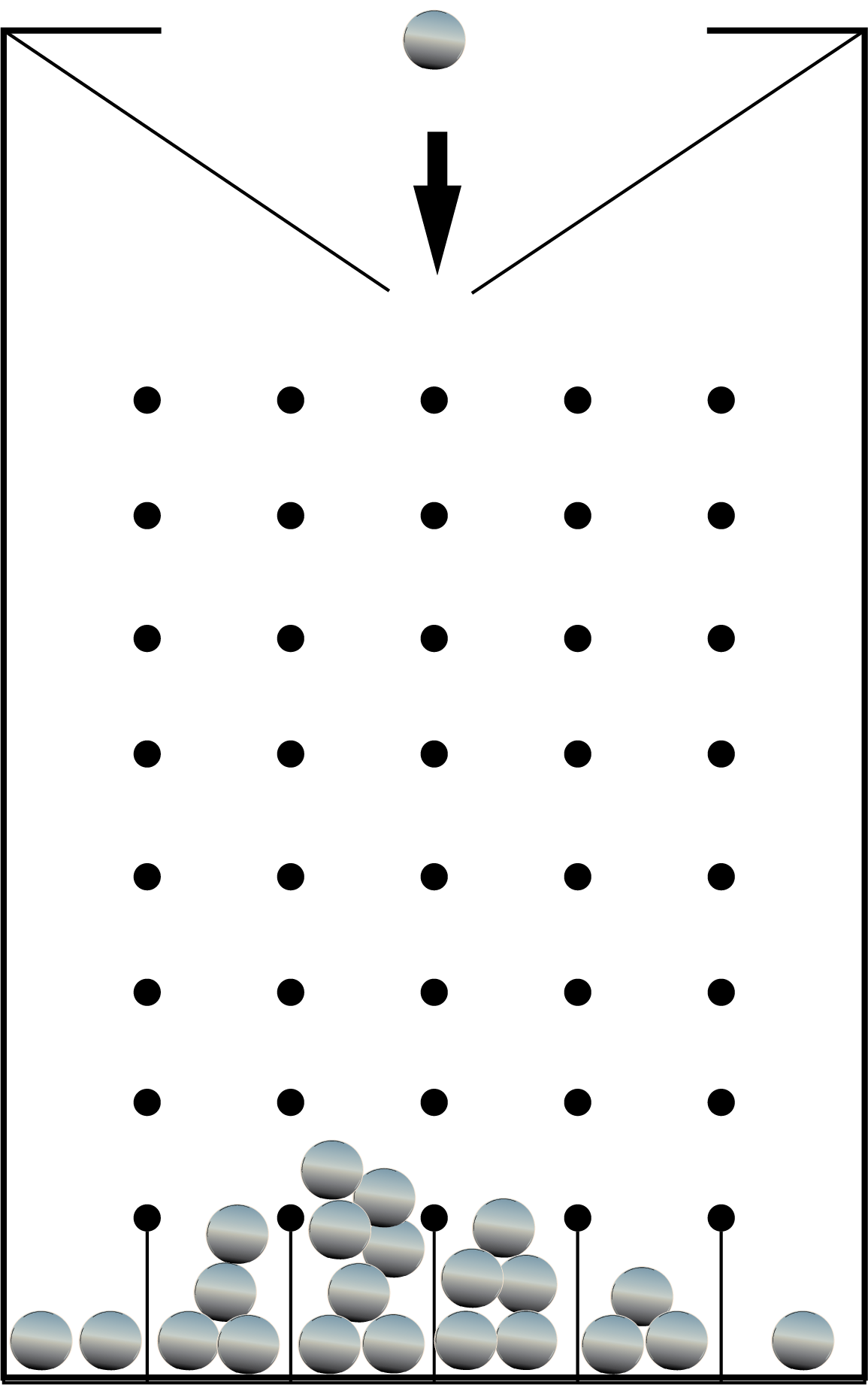
(a) Fixed length classic Galton board.

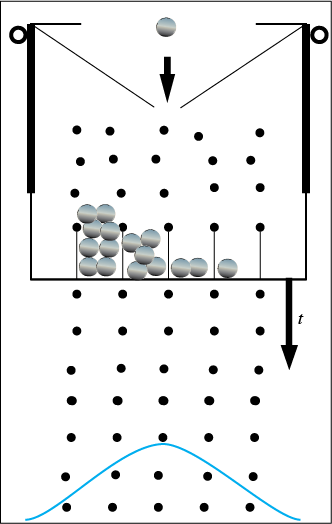
(b) Galton board with changeable length and exaggerated peg-misalignment.

Figure 1: Illustration of our two Galton boards. Not drawn to scale. The longer the board, the longer time the balls spend in the system and the better representative the ensemble mean and variance will be of the underlying PDF, even if it is multi-modal.

For our purposes, each individual ball trajectory represents the time evolution of a single ensemble member and the statistical distribution of the final positions represents the ensemble average for the model. As one observes more and more balls passing through the board, the distribution of final positions at the bottom converges to a pattern that resembles a Gaussian distribution. This convergence is analogous to the ergodic theorem, where the time average (individual ball’s trajectory) converges to the ensemble average (statistical distribution of final positions) over a large number of trials. If we imagine an infinitely long board, the long-time average trajectory for a single ball will be straight down; equivalent to the position of the ensemble mean. Its also worth noting from [17] and [12] that the classic Galton board has been found to possess an ergodic strange attractor, and from [13] that it is not simply a random-walk phenomena. Hence it has useful parallels to weather and climate prediction.

We can play with this idealised ensemble model to examine what can happen if the ergodic assumption fails. The way this can happen is if the system contains multi-modality, in other words, there exist potential wells via certain trajectories into which the balls can stumble from which they are less likely to recover in a certain time-frame. This does not have to be dependant on the different initial conditions, as of course, weather ensemble members “forget" these. In simulations of Galton boards such potential wells have been found to exist, see [1].

Consider a Galton board where we are able to modify the length, thus change the length of time, that the balls must spend in the system. Now let us suppose that the gaps between the pegs are not identically uniform, so at certain points the balls path is impeded slightly more. Locally these act as potential wells, creating multi-modal features. The longer we make the board, the more time the balls will have to explore, enter and escape these potentials. A sufficiently long board (time), and on average the resulting distribution will be our Gaussian again. However, the shorter the board, the more the multi-modal features dominate the picture.

Our model can also be extended to incorporate external forcings. For instance a light fan blowing across the board would shift the distributions, similar to the conceptual model of [30]. The main difference between our Galton board and the picture of [30] is that the latter constrains the system to a bimodal structure which is examined in the long time-limit, whereas our system allows us to imagine any number of modes (depending on the board “resolution" and complexity) and our roller lets us examine long and short time limits. We can now readily see that without enough balls and if the averaging time is too short, the invariance assumption for the distributions is broken. One can also have situations where the balls all get stuck in roughly the same region of the board and so do not explore all the possible trajectories adequately. We suggest that these possibilities may be manifest in ensemble prediction systems and may contribute to the signal to noise paradox. We will next present some theoretical arguments for this conjecture.

2.4 Ergodic error, metrics and RPC

We will now examine how ergodic error could lead to anomalous RPC values and hence the signal-to-noise paradox. To do this we draw on the statistical framework developed by [3]. Let $V(e)$ and $V(o)$ be the respective variances of the ensemble and the observations, then it has been shown that,

$$\sqrt{\frac{V(e)}{V(o)}}<r_{\bar{E}O}\implies RPC>1,$$ (6)

where $r_{\bar{E}O}$ is the Pearson correlation between the observations and the ensemble mean. [3] showed that when we have situations of small correlations, something highly likely for seasonal forecasting, then even minor differences between the observations and ensemble variance gives rise to a signal-to-noise paradox via the above inequality.

We make the conjecture that failure of ergodicity in an ensemble can in some cases lead to these differences. If the ergodic assumption fails for the mean, as defined by equation 4, then it also fails for all statistical moments, including the variance $V(e)$. Mathematically, this is stronger than simply some error, it renders such a variance as meaningless, as without ergodicity, the complete distribution will be different from sampling either from a long time-series of a single member or a complete ensemble. The magnitude of the difference is something which can only be determined by direct computation of the distributions.

Lets try a thought experiment with our windable Galton board in figure 1(b). Suppose the observational reality is that the ball falls straight down, round a zero-mean Gaussian. We could conceive of a situation where our ensemble gets stuck in various potential wells. If we knew each members PDF then we could integrate directly to find the mean, which would weight each member according to the potential well at that instant in time. [3] finds that RPC is especially sensitive to small changes in $r_{\bar{E}O}$, which is highly likely for a multi-modal system, just like our Galton board for short times.

If we look at other simpler physical systems we readily find cases where the failure of the ergodic assumption leads to significant incorrect statistical measures. Examples of such systems include supercooled liquids to glass transitions (see [43]), diffusive processes within the plasma membrane of living cells (see [46]) or general noise processes (see [24]). In each of these cases, handling ensemble averages without due attention to the ergodic assumption leads to in simple terms, wrong answers.

For seasonal predictions, there are multiple factors which could provide ergodic errors. The spatial inhomogeneity of the anomalous RPC values (see e.g. [47] for detailed study), especially over the North Atlantic and Arctic as reported by [5] strongly suggest multimodality is involved, as these regions correlate with well-studied multi-modal behaviour. [41] point out that a multi-modal or regime approach provides an alternative perspective on the paradox. Using a toy bimodal Markov-chain model, they obtain anomalous RPC values when the persistence of the modes is underrepresented. They note specifically the idea that the potential wells for the regimes may be too shallow in the models. We posit that this multimodality, in breaking the ergodic assumption necessary for the ensemble mean and variance, would consequently invalidate interpretation of those statistics, such as RPC.

Our argument, is in some respects analogous to that of [30] who hypothesised the importance of climatic regime states in response to anthropogenic climate change and as [41] remarked, this can also be applied to seasonal predictions. Palmer’s arguments descend from earlier points made by Lorenz with regards to transitive and intransitive systems and climate, see [20], [22] and [23]. There is a close mathematical relationship between ergodicity and transitivity. [8] found that most chaotic systems are also ergodic, although it is possible to be ergodic without being chaotic. The ergodic theorem therefore provides further supporting rigor to the multi-modality paradigm.

3 Next steps

The next step to understanding the connection between ergodicity and anomalous RPC values will be to investigate specific ergodic metrics within different ensemble systems. The Thirumalai–Mountain effective ergodic convergence metric, $\Omega(t)$ measures the effective ergodicity by the difference between the time average of an observable and its ensemble average over the entire system. So for an ensemble of size $n$,

$$\Omega(t)=\frac{1}{n}\sum_{i=1}^{n}\left[f(t)_{i}-E(f(t))\right]^{2},$$ (7)

where the ensemble average is as defined by equation 3. In the long-time limit $\Omega\rightarrow 0$ for an ergodic system. The rate at which this occurs can be used to indicate timescales over which an ergodic approximation might be appropriate. This metric has, as far as we are aware, not been tested before in ensemble prediction systems. However, it is utilised for earthquake forecasting see e.g. [45] and [44], and studies of fluids, see [37]. For other metrics related to ergodicity see [25].

One way to investigate these ideas would be to develop an “ensemble of ensembles". We borrow this idea from a technique for exploring a phase space more completely in direct numerical simulation of the Navier-Stokes equations. At each timestep a small perturbation is made to each member of the ensemble from which several different realisations are computed - the difference between them generating a finite time Lyapunov exponent in the usual way. One could investigate ergodicity by at each time step generating a new ensemble with enough members to compute distributions, such as the Lyapunov spectrum. If the spectrum varies between the ensemble members then this would imply that in a fundamental way, the different ensemble members evolve into different state spaces. Thus interpreting the ensemble mean to be the most likely weather scenario would not be justified and interpreting anomalous RPC values as a paradoxical, incorrect.

One approach to relax the ergodicity constraint but still make use of ensembles is to enforce dynamical invariants. These are quantities that are conserved along the phase space path of the system. For example, in the probability theory for non-equilibrium gravitational systems developed by [31], dynamical invariants are employed with the explicit purpose of not relying ergodicity assumptions. For turbulent fluid systems, the most obvious dynamical invariant would be the Lyapunov spectrum and fractal dimension, besides the more common helicity quantities, such as vorticity.

Recently [32] used the same principle from ergodic theory to developed a weather forecasting machine learning training method. Their algorithm enforced the dynamical invariant of the Lyapunov spectrum and fractal dimension. They tested their neural network on the classic Lorenz 1996 chaotic dynamical system. Including the ergodic constraints improved the forecast skill of the neural network. We speculate that the RPC value will be improved for long-range forecasts if these invariant constraints can be carefully applied to the ensembles. Each observable should have its own invariant measure for the ergodic theorem to hold for the ensemble. However, applying such an invariant might also constrain the ensemble in an unhelpful way, as it is possible that the real world observable does not obey the invariant anyway.

CONFLICT OF INTEREST

The author declares no conflict of interest.

References

- Ahmed et al. [2022] Ahmed, J., Chumley, T., Cook, S., Cox, C., Grant, H., Petela, N., Rothrock, B. and Xhafaj, R. (2022) Dynamics of the no-slip galton board. URL: https://arxiv.org/abs/2208.07790.
- Birkhoff [1931] Birkhoff, G. D. (1931) Proof of the ergodic theorem. Proceedings of the National Academy of Sciences of the United States of America, 17, 656–660. URL: http://www.jstor.org/stable/86016.
- Bröcker et al. [2023] Bröcker, J., Charlton–Perez, A. J. and Weisheimer, A. (2023) A statistical perspective on the signal-to-noise paradox. Quarterly Journal of the Royal Meteorological Society, 149, 911–923. URL: https://rmets.onlinelibrary.wiley.com/doi/abs/10.1002/qj.4440.
- Charlton-Perez et al. [2019] Charlton-Perez, A., Bröcker, J., Stockdale, T. N. and Johnson, S. J. (2019) When and where do ecmwf seasonal forecast systems exhibit anomalously low signal-to-noise ratio? Quarterly Journal of the Royal Meteorological Society, 145, 3466–3478. URL: https://doi.org/10.1002/qj.3631.
- Cottrell et al. [2024] Cottrell, F. M., Screen, J. A. and Scaife, A. A. (2024) Signal-to-noise errors in free-running atmospheric simulations and their dependence on model resolution. Atmospheric Science Letters, n/a, e1212. URL: https://rmets.onlinelibrary.wiley.com/doi/abs/10.1002/asl.1212.
- Dunstone et al. [2023] Dunstone, N., Smith, D. M., Hardiman, S. C., Hermanson, L., Ineson, S., Kay, G., Li, C., Lockwood, J. F., Scaife, A. A., Thornton, H., Ting, M. and Wang, L. (2023) Skilful predictions of the summer north atlantic oscillation. Communications Earth & Environment, 4, 409. URL: https://doi.org/10.1038/s43247-023-01063-2.
- Eade et al. [2014] Eade, R., Smith, D., Scaife, A. A., Wallace, E., Dunstone, N., Hermanson, L. and Robinson, N. (2014) Do seasonal-to-decadal climate predictions underestimate the predictability of the real world? Geophysical research letters, 41, 5620–5628. URL: https://doi.org/10.1002/2014gl061146.
- Eckmann and Ruelle [1985] Eckmann, J. P. and Ruelle, D. (1985) Ergodic theory of chaos and strange attractors. Rev. Mod. Phys., 57, 617–656. URL: https://link.aps.org/doi/10.1103/RevModPhys.57.617.
- Epstein [1969] Epstein, E. S. (1969) Stochastic dynamic prediction. Tellus, 21, 739–759.
- Galton [1889] Galton, F. (1889) Natural Inheritance. No. v. 42; v. 590 in Natural Inheritance. Macmillan.
- Hardiman et al. [2022] Hardiman, S. C., Dunstone, N. J., Scaife, A. A., Smith, D. M., Comer, R., Nie, Y. and Ren, H.-L. (2022) Missing eddy feedback may explain weak signal-to-noise ratios in climate predictions. npj Climate and Atmospheric Science, 5, 57.
- Hoover and Moran [1992] Hoover, W. G. and Moran, B. (1992) Viscous attractor for the galton board. Chaos, 2, 599–602.
- Judd [2007] Judd, K. (2007) Galton’s quincunx: Random walk or chaos? International Journal of Bifurcation and Chaos, 17, 4463–4469.
- Knight et al. [2022] Knight, J. R., Scaife, A. A. and Maidens, A. (2022) An extratropical contribution to the signal-to-noise paradox in seasonal climate prediction. Geophysical Research Letters, 49, e2022GL100471. URL: https://agupubs.onlinelibrary.wiley.com/doi/abs/10.1029/2022GL100471. E2022GL100471 2022GL100471.
- Kong [2019] Kong, T. (2019) Ergodic theory, entropy and application to statistical mechanics. URL: https://api.semanticscholar.org/CorpusID:208176466.
- Kumar [2009] Kumar, A. (2009) Finite samples and uncertainty estimates for skill measures for seasonal prediction. Monthly Weather Review, 137, 2622–2631.
- Kumičák [2000] Kumičák, J. (2000) Galton board as a model for fluctuations. In Unsolved Problems of Noise and Fluctuations: UPoN’99: Second International Conference, vol. 511 of American Institute of Physics Conference Series, 144–149.
- Leutbecher [2019] Leutbecher, M. (2019) Ensemble size: How suboptimal is less than infinity? Quarterly Journal of the Royal Meteorological Society, 145, 107–128. URL: https://rmets.onlinelibrary.wiley.com/doi/abs/10.1002/qj.3387.
- Lorenz [1963] Lorenz, E. N. (1963) Deterministic nonperiodic flow. Journal of atmospheric sciences, 20, 130–141.
- Lorenz [1968] — (1968) Climatic Determinism, 1–3. Boston, MA: American Meteorological Society. URL: https://doi.org/10.1007/978-1-935704-38-6_1.
- Lorenz [1969] — (1969) The predictability of a flow which possesses many scales of motion. Tellus, 21, 289–307.
- Lorenz [1976] — (1976) Nondeterministic theories of climatic change. Quaternary Research, 6, 495–506. URL: https://www.sciencedirect.com/science/article/pii/0033589476900223.
- Lorenz [1990] — (1990) Can chaos and intransitivity lead to interannual variability? Tellus A, 42, 378–389. URL: https://onlinelibrary.wiley.com/doi/abs/10.1034/j.1600-0870.1990.t01-2-00005.x.
- Mangalam and Kelty-Stephen [2022] Mangalam, M. and Kelty-Stephen, D. G. (2022) Ergodic descriptors of non-ergodic stochastic processes. Journal of The Royal Society Interface, 19, 20220095. URL: https://royalsocietypublishing.org/doi/abs/10.1098/rsif.2022.0095.
- Mathew and Mezić [2011] Mathew, G. and Mezić, I. (2011) Metrics for ergodicity and design of ergodic dynamics for multi-agent systems. Physica D: Nonlinear Phenomena, 240, 432–442. URL: https://www.sciencedirect.com/science/article/pii/S016727891000285X.
- Murphy and Palmer [1986] Murphy, J. and Palmer, T. (1986) Experimental monthly long-range forecasts for the united-kingdom. 2. a real-time long-range forecast by an ensemble of numerical integrations. Meteorological Magazine, 115.
- O’Reilly et al. [2019] O’Reilly, C. H., Weisheimer, A., Woollings, T., Gray, L. J. and MacLeod, D. (2019) The importance of stratospheric initial conditions for winter north atlantic oscillation predictability and implications for the signal-to-noise paradox. Quarterly Journal of the Royal Meteorological Society, 145, 131–146. URL: https://rmets.onlinelibrary.wiley.com/doi/abs/10.1002/qj.3413.
- Ossó et al. [2020] Ossó, A., Sutton, R., Shaffrey, L. and Dong, B. (2020) Development, amplification, and decay of atlantic/european summer weather patterns linked to spring north atlantic sea surface temperatures. Journal of Climate, 33, 5939–5951.
- Palmer and Hagedorn [2006] Palmer, T. and Hagedorn, R. (2006) Predictability of Weather and Climate. Cambridge University Press.
- Palmer [1999] Palmer, T. N. (1999) A nonlinear dynamical perspective on climate prediction. Journal of Climate, 12, 575 – 591. URL: https://journals.ametsoc.org/view/journals/clim/12/2/1520-0442_1999_012_0575_andpoc_2.0.co_2.xml.
- Peñarrubia [2015] Peñarrubia, J. (2015) A probability theory for non-equilibrium gravitational systems. Monthly Notices of the Royal Astronomical Society, 451, 3537–3550. URL: https://doi.org/10.1093/mnras/stv1146.
- Platt et al. [2023] Platt, J. A., Penny, S. G., Smith, T. A., Chen, T.-C. and Abarbanel, H. D. I. (2023) Constraining chaos: Enforcing dynamical invariants in the training of reservoir computers. Chaos: An Interdisciplinary Journal of Nonlinear Science, 33, 103107. URL: https://doi.org/10.1063/5.0156999.
- Scaife et al. [2014] Scaife, A. A., Arribas, A., Blockley, E. W., Brookshaw, A., Clark, R. T., Dunstone, N., Eade, R., Fereday, D., Folland, C. K., Gordon, M., Hermanson, L., Knight, J., Lea, D. J., MacLachlan, C., Maidens, A., Martin, M., Peterson, A., Smith, D., Vellinga, M., Wallace, E., Waters, J. and Williams, A. J. (2014) Skillful long-range prediction of european and north american winters. Geophysical Research Letters, 41, 2514–2519. URL: https://doi.org/10.1002/2014gl059637.
- Scaife et al. [2019] Scaife, A. A., Camp, J., Comer, R., Davis, P., Dunstone, N., Gordon, M., MacLachlan, C., Martin, N., Nie, Y., Ren, H.-L. et al. (2019) Does increased atmospheric resolution improve seasonal climate predictions? Atmospheric Science Letters, 20, e922.
- Scaife and Smith [2018] Scaife, A. A. and Smith, D. (2018) A signal-to-noise paradox in climate science. npj Climate and Atmospheric Science, 1, 28. URL: https://doi.org/10.1038/s41612-018-0038-4.
- Siegert et al. [2015] Siegert, S., Stephenson, D. B., Sansom, P. G., Scaife, A. A., Eade, R. and Arribas, A. (2015) A Bayesian Framework for Verification and Recalibration of Ensemble Forecasts: How Uncertain is NAO Predictability? Journal of Climate, 29, 995–1012. URL: https://doi.org/10.1175/JCLI-D-15-0196.1.
- de Souza and Wales [2005] de Souza, V. K. and Wales, D. J. (2005) Diagnosing broken ergodicity using an energy fluctuation metric. The Journal of Chemical Physics, 123, 134504. URL: https://doi.org/10.1063/1.2035080.
- Stockdale et al. [2015] Stockdale, T. N., Molteni, F. and Ferranti, L. (2015) Atmospheric initial conditions and the predictability of the arctic oscillation. Geophysical Research Letters, 42, 1173–1179. URL: https://doi.org/10.1002/2014gl062681.
- Strommen [2020] Strommen, K. (2020) Jet latitude regimes and the predictability of the north atlantic oscillation. Quarterly Journal of the Royal Meteorological Society, 146, 2368–2391.
- Strommen et al. [2023] Strommen, K., MacRae, M. and Christensen, H. (2023) On the relationship between reliability diagrams and the “signal-to-noise paradox”. Geophysical Research Letters, 50, e2023GL103710. URL: https://agupubs.onlinelibrary.wiley.com/doi/abs/10.1029/2023GL103710. E2023GL103710 2023GL103710.
- Strommen and Palmer [2018] Strommen, K. and Palmer, T. (2018) Signal and noise in regime systems: A hypothesis on the predictability of the north atlantic oscillation. Quarterly Journal of the Royal Meteorological Society, 145, 147–163. URL: https://doi.org/10.1002/qj.3414.
- Tantet [2016] Tantet, A. J. J. (2016) Ergodic theory of climate: variability, stability and response. Ph.D. thesis, Utrecht University.
- Thirumalai et al. [1989] Thirumalai, D., Mountain, R. D. and Kirkpatrick, T. R. (1989) Ergodic behavior in supercooled liquids and in glasses. Phys. Rev. A, 39, 3563–3574. URL: https://link.aps.org/doi/10.1103/PhysRevA.39.3563.
- Tiampo et al. [2007] Tiampo, K. F., Rundle, J. B., Klein, W., Holliday, J., Sá Martins, J. S. and Ferguson, C. D. (2007) Ergodicity in natural earthquake fault networks. Phys. Rev. E, 75, 066107. URL: https://link.aps.org/doi/10.1103/PhysRevE.75.066107.
- Tiampo et al. [2003] Tiampo, K. F., Rundle, J. B., Klein, W., Martins, J. S. S. and Ferguson, C. D. (2003) Ergodic dynamics in a natural threshold system. Phys. Rev. Lett., 91, 238501. URL: https://link.aps.org/doi/10.1103/PhysRevLett.91.238501.
- Weigel et al. [2011] Weigel, A. V., Simon, B., Tamkun, M. M. and Krapf, D. (2011) Ergodic and nonergodic processes coexist in the plasma membrane as observed by single-molecule tracking. Proc Natl Acad Sci U S A, 108, 6438–6443.
- Weisheimer et al. [2019] Weisheimer, A., Decremer, D., MacLeod, D., O’Reilly, C. H., Stockdale, T. N., Johnson, S. J. and Palmer, T. (2019) How confident are predictability estimates of the winter north atlantic oscillation. Quarterly Journal of the Royal Meteorological Society, 145, 140–159. URL: https://doi.org/10.1002/qj.3446.
- Zhang [2019] Zhang, Wei; Kirtman, B. P. (2019) Understanding the signal-to-noise paradox with a simple markov model. Geophysical Research Letters, 46, 13308–13317. URL: https://doi.org/10.1029/2019gl085159.