Robust Elastic Net Estimators for High Dimensional Generalized Linear Models

Abstract

Robust estimators for Generalized Linear Models (GLMs) are not easy to develop because of the nature of the distributions involved. Recently, there has been an increasing interest in this topic, especially in the presence of a possibly large number of explanatory variables. Transformed M-estimators (MT) are a natural way to extend the methodology of M-estimators to the class of GLMs and to obtain robust methods. We introduce a penalized version of MT-estimators in order to deal with high-dimensional data. We prove, under appropriate assumptions, consistency and asymptotic normality of this new class of estimators. The theory is developed for redescending $\rho$-functions and Elastic Net penalization. An iterative re-weighted least squares algorithm is given, together with a procedure to initialize it. The latter is of particular importance, since the estimating equations might have multiple roots. We illustrate the performance of this new method for the Poisson family under several type of contaminations in a Monte Carlo experiment and in an example based on a real dataset.

Keywords: high-dimension, GLMs, MT-estimators, penalized methods, robustness.

1 Introduction

Generalized linear models (GLMs) are an important tool in data analysis. In high dimensional problems, traditional methods fail, because they are based on the assumption that the number of observations is larger than the number of covariates. The problem of high dimensional data has been widely studied and penalized procedures have been proposed to address it. For linear models, Hoerl and Kennard [1970] have proposed the Ridge, Tibshirani [1996] the Lasso and Zou and Hastie [2005] the Elastic Net, while Friedman et al. [2010] have studied their generalization to GLMs. Fan and Li [2001] have introduced the smoothly clipped absolute deviation (SCAD) penalty. Penalized estimators for linear regression have also been studied by Knight and Fu [2000] and Zou [2006].

All the mentioned proposals have a very good performance if all the observations follow the assumed model. However, if a small proportion of the observed data are atypical, they become completely unreliable.

Robust estimators for high dimensional linear models have been proposed by Maronna [2011] and Smucler and Yohai [2017], among others, while Bianco et al. [2023] have proposed penalized robust estimators for logistic regression. Avella-Medina and Ronchetti [2018] have introduced a family of penalized robust estimators for GLMs, with the aim of performing variable selection. Another proposal for robust variable selection in GLMs was given by Salamwade and Sakate [2021], who introduced penalized MT-estimators and proved their oracle properties. The family of penalty functions considered by these last two papers includes the SCAD and the Lasso penalties but does not include the Ridge penalty or other Elastic Net penalties. Moreover, neither the simulation study nor the real examples in Salamwade and Sakate [2021] deal with high dimensional data. In fact, Agostinelli et al. [2019] showed that a new computational method is required for this type of data and in particular that the initial estimators are extremely influential to the performance of the whole procedure.

In this paper we introduce penalized MT-estimators based on the Elastic Net penalty function. We study their theoretical properties such as consistency and asymptotic normality under suitable assumptions. We also introduce a computational algorithm and a procedure to obtain an initial estimate. The results of an extensive Monte Carlo study are presented, as well as an application to a real data set in which we seek to predict the length of hospital stay of patients using several covariates.

The rest of the paper is organized as follows. Section 2 reviews the definition of MT-estimators for GLMs, while Section 3 introduces their penalized version based on the Elastic Net penalty function. Section 4 discusses the selection of the penalty parameters by Information Criteria or Cross-Validation, while Section 5 provide asymptotic results. Section 6 and 7 contain the Monte Carlo setting, a summary of its results and an the application example. Section 8 provides some concluding remarks. Appendix A contains the complete proofs of the theorems given in Section 5, whereas Appendix B provides details on how to obtain a robust starting value and the description of the Iterative Re-Weighted Least Squares (IRWLS) algorithm. Finally, Appendix C reports further results of the Monte Carlo experiment.

2 M-estimators based on transformations

Let $(y,\mathbf{x})$ be a random vector of dimension $p+2$ and $F=F(.,\mu,\phi)$ a distribution function depending on two parameters $\mu$ and $\phi$, with $\mu\in(\mu_{1},\mu_{2})$ where $\mu_{i}$ can be $\pm\infty$ and $\phi>0$. We say that $(y,\mathbf{x})$ follow a GLMs with parameter $\boldsymbol{\beta}$, link function $g$ and distribution function $F$ if

$$y|\mathbf{x}\sim F(.,\mu,\phi),\qquad g(\mu)=\eta=\mathbf{x}^{\top}\boldsymbol{\beta},$$ (1)

where $\boldsymbol{\beta}=(\beta_{0},\boldsymbol{\beta_{1}}^{\top})^{\top}$ is the parameter of the linear predictor $\eta$, $\beta_{0}\in\mathbb{R}$, $\boldsymbol{\beta_{1}}=(\beta_{1},\dots,\beta_{p})^{\top}\in\mathbb{R}^{p}$, $\mathbf{x}=(1,\mathbf{z}^{\top})^{\top}$, $\mathbf{z}=(x_{1},\ldots,x_{p})^{\top}\in\mathbb{R}^{p}$ and $\phi$ is a nuisance scale parameter which is assumed to be known. We assume that $g$ is defined on $(\mu_{1},\mu_{2})$, and that it is continuous and strictly increasing. We also assume that $\mathop{\lim_{\mu\rightarrow\mu_{1}}}g(\mu)=-\infty$ and $\mathop{\lim_{\mu\rightarrow\mu_{2}}}g(\mu)=+\infty$. Let $t$ be a variance stabilizing transformation, that is, such that $\operatorname{\mathbb{V}ar}(t(y))\approx a(\phi)$ is approximately constant and $a$ is a known function. We define

$$L(\boldsymbol{\beta})=\operatorname{\mathbb{E}}_{\boldsymbol{\beta}_{*}}\left(\rho\left(\frac{t(y)-m(g^{-1}(\mathbf{x}^{\top}\boldsymbol{\beta}))}{\sqrt{a(\phi)}}\right)\right)$$ (2)

and the $m$ function is given by

$$m(\mu)=\arg\min_{\gamma}\operatorname{\mathbb{E}}_{\mu}\left(\rho\left(\frac{t(y)-\gamma}{\sqrt{a(\phi)}}\right)\right),$$ (3)

where $\rho$ is a bounded $\rho$-function such as Tukey’s bisquare function (see Section 5 for the definition of a $\rho$-function) and $t$ is a variance stabilizing transformation; for instance, in the Poisson case $t(x)=\sqrt{x}$. The function $m$ is necessary to ensure the Fisher consistency of the estimator. We assume that this function is uniquely defined for all $\mu$. We denote by $mg^{-1}$ the composition $m\circ g^{-1}$.

By $\operatorname{\mathbb{E}}_{\boldsymbol{\beta}_{*}}(h(y,\mathbf{x}))$ we denote the expectation of $h(y,\mathbf{x})$, when $(y,\mathbf{x})$ follows a GLMs with parameter $\boldsymbol{\beta}_{*}$, as defined in (1). This notation is used in the definition of $L$ in order to emphasize the different roles of $\boldsymbol{\beta}$ and $\boldsymbol{\beta}_{*}$. In the sequel, we will denote it either by $\operatorname{\mathbb{E}}_{\boldsymbol{\beta}_{*}}(h(y,\mathbf{x}))$ or simply by $\operatorname{\mathbb{E}}(h(y,\mathbf{x}))$ when the distribution of $(y,\mathbf{x})$ is clear.

Introduced by Valdora and Yohai [2014], M-estimators based on transformations (MT), are the finite sample version of (2). Given an independent and identically distributed (i.i.d.) sample $(y_{1},\mathbf{x}_{1}),\ldots,(y_{n},\mathbf{x}_{n})$ of size $n$, we define

$$L_{n}(\boldsymbol{\beta})=\frac{1}{n}\sum_{i=1}^{n}\rho\left(\frac{t(y_{i})-mg^{-1}\left(\mathbf{x}_{i}^{\top}\boldsymbol{\beta}\right)}{\sqrt{a(\phi)}}\right)$$ (4)

and the MT-estimator is $\tilde{\boldsymbol{\beta}}_{n}=\arg\min_{\boldsymbol{\beta}}L_{n}(\boldsymbol{\beta})$.

Taking $\rho(x)=x^{2}$ we get a least squares estimate based on transformations (LST) for GLMs:

$$\tilde{\boldsymbol{\beta}}_{LS}=\arg\min_{\boldsymbol{\beta}}\sum_{i=1}^{n}\left(t(y_{i})-m_{LS}\left(g^{-1}(\mathbf{x}_{i}^{\top}\boldsymbol{\beta})\right)\right)^{2},$$ (5)

where $m_{LS}(\mu)=\mathbb{E}_{\mu}(t(y))$. Hence, MT-estimators can be seen as a robustification of LST-estimators. LST- and MT-estimators are investigated in Agostinelli et al. [2019], where an initial estimator based on the idea of Peña and Yohai [1999] is proposed and an IRWLS algorithm to solve the minimization problem is studied.

3 Penalized MT-estimators for Generalized Linear Models

Consider the following penalized objective function

$$\hat{L}_{n}(\boldsymbol{\beta})=\frac{1}{2n}\sum_{i=1}^{n}\rho\left(\frac{t(y_{i})-mg^{-1}\left(\mathbf{x}_{i}^{\top}\boldsymbol{\beta}\right)}{\sqrt{a(\phi)}}\right)+\lambda P_{\alpha}(\boldsymbol{\beta}),$$ (6)

where $P_{\alpha}(\boldsymbol{\beta})$ is a penalization term depending on the vector $\boldsymbol{\beta}$, and $\alpha$ and $\lambda$ are penalization parameters. We define penalized MT-estimators as

$$\hat{\boldsymbol{\beta}}_{n}=\hat{\boldsymbol{\beta}}_{n,\lambda,\alpha}=\arg\min_{\boldsymbol{\beta}}\hat{L}_{n}(\boldsymbol{\beta}).$$ (7)

For instance, as in Zou and Hastie [2005], let

$$P_{\alpha}(\boldsymbol{\beta}) =(1-\alpha)\frac{1}{2}\|\boldsymbol{\beta_{1}}\|^{2}_{2}+\alpha\|\boldsymbol{\beta_{1}}\|_{1}$$ (8)

$$=\sum_{j=1}^{p}\frac{1}{2}(1-\alpha)\beta_{j}^{2}+\alpha|\beta_{j}|$$

be the Elastic Net penalty, which corresponds to the Ridge penalty for $\alpha=0$ and to the Lasso penalty for $\alpha=1$. Notice that we are not penalizing the intercept $\beta_{0}$. However, the theory we devolope also applies to the case in which the intercept is penalized.

For the computation of these estimators we use an IRLWS algorithm which is described in Appendix B. The use of a redescending $\rho$ function, essential to get a high breakdown point robust estimator, leads to a non convex optimization problem, in which the loss function may have several local minima. For this reason, the choice of the initial point for the IRWLS algorithm is crucial. In particular, we need to start the iterations at an estimator that is already close to the global minimum in order to avoid convergence to a different local minimum. In low dimensions, solutions to this problem are often obtained by the subsampling procedure e.g., the fast S-estimator for regression of Salibian-Barrera and Yohai [2006]. Penalized robust procedures can use the same approach e.g., in Alfons et al. [2013]. However, when the dimension of the problem becomes large, the number of sub-samples one needs to explore in order to find a good initial estimator becomes soon computationally infeasible. For this reason, we propose deterministic algorithm, reported in Appendix B, inspired by Peña and Yohai [1999]. A similar algorithm is introduced in Agostinelli et al. [2019] for the unpenalized MT-estimators, and it is proved to be highly robust and computationally efficientos de.

4 Selection of the penalty parameters

Robust selection of the penalty parameters can be performed using information like criteria, such as AIC or BIC, or by Cross-Validation. Information criteria are of the form

$$IC(\lambda,\alpha)=\text{Goodness of the fit}+\text{Complexity Penalty}\times\text{Degree of Freedom}.$$

For penalized methods the degrees of freedom, which measure the complexity of the model, have been studied extensively; see e.g. [Friedman et al., 2001, Zou et al., 2007, Tibshirani and Taylor, 2012] and the references therein. For the Elastic Net penalty the degrees of freedom are based on an “equivalent projection” matrix $\mathbf{H}$ that in our context is given by

$$\mathbf{H}=\sqrt{\mathbf{W}}\mathbf{X}_{\mathcal{A}}(\mathbf{X}_{\mathcal{A}}^{\top}\mathbf{W}\mathbf{X}_{\mathcal{A}}+\lambda(1-\alpha)\mathbf{I}_{p})^{-1}\mathbf{X}_{\mathcal{A}}^{\top}\sqrt{\mathbf{W}}$$ (9)

where $\mathbf{W}$ is a diagonal matrix of weights given by $\mathbf{w}^{2}(\mathbf{x}_{i}^{\top}\hat{\boldsymbol{\beta}}_{n})\mathbf{w}^{\ast}(\mathbf{x}_{i}^{\top}\hat{\boldsymbol{\beta}}_{n})$ ($i=1,\ldots,n$) defined in equation (31) in Appendix B and $\mathbf{X}_{\mathcal{A}}$ is the matrix containing only the covariates corresponding to the active set $\mathcal{A}$, which is defined as the set of covariates with estimated coefficients different from 0.

Then, the equivalent degrees of freedom are given by

$$\text{df}(\lambda,\alpha)=\operatorname{tr}(\mathbf{H})$$

which leads to the definitions of their penalized versions

$$AIC(\lambda,\alpha) =\hat{L}_{n}(\hat{\boldsymbol{\beta}}_{n})+2\operatorname{df}(\lambda,\alpha)$$

$$BIC(\lambda,\alpha) =\hat{L}_{n}(\hat{\boldsymbol{\beta}}_{n})+\log(n)\operatorname{df}(\lambda,\alpha)$$

and to the choice of $\lambda$ and $\alpha$ that minimise these measures.

Alternatively, we can select the penalty parameters by cross-validation. We first divide the data into $K$ disjoint subsets of approximately the same number of observations. Let $c_{1},\dots,c_{K}$ be the number of observations in each of the subsets. Let $\hat{\boldsymbol{\beta}}^{(j)}_{\lambda,\alpha}$ be an estimator of $\boldsymbol{\beta}$ computed with penalty parameters $(\lambda,\alpha)$ and without using the observations of the $j$-th subset. The robust cross-validation criterion chooses $\lambda,\alpha$ that minimize

$$\operatorname{RCV}(\lambda,\alpha)=\frac{1}{n}\sum_{j=1}^{K}c_{j}\hat{L}_{n}^{(j)}(\hat{\boldsymbol{\beta}}^{(j)}_{\lambda,\alpha})$$

where $\hat{L}_{n}^{(j)}$ is the loss function defined in (6) for the observations belonging to the $j$-th cross-validation subset.

5 Asymptotic results

In this section we discuss some asymptotic properties of the penalized MT-estimators. Throughout this and the following section, we assume $(y_{1},\mathbf{x}_{1}),\dots,$ $(y_{n},\mathbf{x}_{n})$ and $(y,\mathbf{x})$ to be i.i.d. random vectors following a GLMs with parameter $\boldsymbol{\beta}_{*}$, distribution $F$ and continuous and strictly increasing link function $g$ and we consider the estimator $\hat{\boldsymbol{\beta}}_{n}$ defined in (7). The following assumptions are needed to prove consistency of the penalized MT-estimators, and they are the same used for the MT-estimators, see Valdora and Yohai [2014].

• $\sup_{\mu}\operatorname{\mathbb{V}ar}_{\mu}(t(y))=A<\infty$.

• $\ m(\mu)$ is univocally defined for all $\mu$ and $\mu_{1}<\mu_{2}$ implies $m(\mu_{1})<m(\mu_{2})$.

• $F(\mu,\phi)$ is continuous in $\mu$ and $\phi$.

• Suppose that $\mu_{1}<\mu_{2}$, $X_{1}\sim F(\mu_{1},\phi)$ and $X_{2}\sim F(\mu_{2},\phi)$ then $X_{1}$ is stochastically smaller $X_{2}$.

• The function $t$ is strictly increasing and continuous.

A function is a $\rho$-function if it satisfies the following assumptions

• $\rho(u)\geq$ $0$, $\rho(0)=0$ and $\rho(u)=\rho(-u)$.

• $\lim_{u\rightarrow\infty}\rho(u)=a<\infty$. Without loss of generality we will assume $a=1$.

• $0\leq u<v$ implies $\rho(u)\leq\rho(v)$.

• $0\leq u<v$ and $\rho(u)<1$ implies $\rho(u)<\rho(v)$.

• $\rho$ is continuous.

• Let $A$ be as in A1, then there exists $\eta$ such that $\rho(A^{1/2}+\eta)<1$.

We also consider the following assumption on the distribution of the covariate vector $\mathbf{x}$

• Let $S=\left\{\mathbf{t}\in\mathbb{R}^{p+1}:||\mathbf{t}||=1\right\}$, then $\inf\left\{\mathbb{P}\left(\mathbf{t}^{\top}\mathbf{x}\neq\mathbf{0}\right),\mathbf{t}\in S\right\}>0$.

The following lemma has been proved in Valdora and Yohai [2014], as part of the proof of their Theorem 1. We include it here because it is needed to state the next assumption.

Lemma 1

Assume A1-A5 and B1-B7, then

$$\tau=\mathbb{E}_{\boldsymbol{\beta}_{*}}\left(\lim_{\zeta\rightarrow\infty}\rho\left(\frac{t(y)-mg^{-1}(\zeta\mathbf{x}^{\top}\mathbf{t})}{\sqrt{a(\phi)}}\right)\right)-L(\boldsymbol{\beta}_{*})>0.$$ (10)

The following assumption on the distribution of the covariate vector $\mathbf{x}$, which is a little stronger than B7, is needed for consistency.

• Let $\tau$ be defined as in (10), then $\inf\left\{\mathbb{P}\left(\mathbf{t}^{\top}\mathbf{x}\neq\mathbf{0}\right),\mathbf{t}\in S\right\}>1-\tau$.

Note that assumption B8 is trivially verified if $\mathbf{x}=(1,\mathbf{z})$ and $\mathbf{z}$ has a density.

The following theorem establishes the strong consistency of penalized MT-estimators. All the proofs are deferred to Appendix A.

Theorem 2 (Consistency)

Assume A1-A5 and B1-B6 and B8 hold, and that $\lambda_{n}P_{\alpha_{n}}(\boldsymbol{\beta}_{*})\stackrel{{\scriptstyle a.s.}}{{\longrightarrow}}0$ when $n\rightarrow\infty$. Then $\hat{\boldsymbol{\beta}}_{n}$ is strongly consistent for $\boldsymbol{\beta}_{*}$.

The following assumptions will be needed to derive the order of convergence and the asymptotic normality of the proposed estimators. It is worth mentioning that Lemma 5 in Valdora and Yohai [2014] proves that the function $m$ is twice differentiable, since this is needed for assumption C4.

• $F_{\mu}$ has three continuous and bounded derivatives as a function of $\mu$ and the link function $g(\mu)$ is twice continuously differentiable.

• $\rho$ has three continuous and bounded derivatives. We write $\psi=\rho^{\prime}$.

• $\operatorname{\mathbb{E}}_{\mu}(\psi^{\prime}(t(y)-m(\mu)))\neq 0$ for all $\mu$.

• Let $\boldsymbol{\Psi}(y,\mathbf{x},\boldsymbol{\beta})$ be the derivative of $\rho((t(y)-mg^{-1}(\mathbf{x}^{\top}\boldsymbol{\beta}))/\sqrt{a(\phi)})$ with respect to $\boldsymbol{\beta}$ and $\mathbf{J}(y,\mathbf{x},\boldsymbol{\beta})$ be the Hessian matrix. There exists $\eta>0$ such that $\operatorname{\mathbb{E}}\left(\sup_{||\boldsymbol{\beta}-\boldsymbol{\beta}_{*}||\leq\eta}\left|J^{j,k}(y,\mathbf{x},\boldsymbol{\beta})\right|\right)<\infty$, for all $1\leq j,k\leq p,$ where $||\cdot||$ denotes the $L_{2}$ norm, and $\operatorname{\mathbb{E}}(\mathbf{J}(y,\mathbf{x},\boldsymbol{\beta}_{*}))$ is non singular.

Theorem 3 (Order of convergence)

Assume A1-A5, B1-B6, B8, C1-C4 and $\operatorname{\mathbb{E}}(||\mathbf{x}||^{2})<\infty$. Then $||\hat{\boldsymbol{\beta}}_{n}-\boldsymbol{\beta}_{*}||=O_{P}(\lambda_{n}+1/\sqrt{n})$. Hence, if $\lambda_{n}=O_{P}(1/\sqrt{n})$, we have that $||\hat{\boldsymbol{\beta}}_{n}-\boldsymbol{\beta}_{*}||=O_{P}(1/\sqrt{n})$, while if $\lambda_{n}\sqrt{n}\rightarrow\infty$, $||\hat{\boldsymbol{\beta}}_{n}-\boldsymbol{\beta}_{*}||=O_{P}(\lambda_{n})$.

In order to establish the asymptotic normality of penalized MT-estimators we define the expectation of the Hessian matrix $\mathbf{J}$ and the variance of the gradient vector $\boldsymbol{\Psi}$ together with their empirical versions

$$\mathbf{A} =\operatorname{\mathbb{E}}_{\boldsymbol{\beta}_{*}}(\mathbf{J}(y,\mathbf{x},\boldsymbol{\beta}_{*})), \mathbf{B} =\operatorname{\mathbb{E}}_{\boldsymbol{\beta}_{*}}(\boldsymbol{\Psi}(y,\mathbf{x},\boldsymbol{\beta}_{*})\boldsymbol{\Psi}(y,\mathbf{x},\boldsymbol{\beta}_{*})^{\top}),$$ (11)

$$\mathbf{A}_{n}(\boldsymbol{\beta}) =\frac{1}{n}\sum_{i=1}^{n}\mathbf{J}(y_{i},\mathbf{x}_{i},\boldsymbol{\beta}), \mathbf{B}_{n}(\boldsymbol{\beta}) =\frac{1}{n}\sum_{i=1}^{n}\boldsymbol{\Psi}(y_{i},\mathbf{x}_{i},\boldsymbol{\beta})\boldsymbol{\Psi}(y_{i},\mathbf{x}_{i},\boldsymbol{\beta})^{\top}.$$

Theorem 4 (Asymptotic normality)

Assume C1-C4 hold. Furthermore assume that $\operatorname{\mathbb{E}}(||\mathbf{x}||^{2})<\infty$, $\sqrt{n}(\hat{\boldsymbol{\beta}}_{n}-\boldsymbol{\beta}_{*})=O_{P}(1)$ and that $\sqrt{n}\lambda_{n}\stackrel{{\scriptstyle p}}{{\longrightarrow}}b$, with $0\leq b<+\infty$. Then, if $\left\|\boldsymbol{\beta}_{*}\right\|\neq 0,\sqrt{n}(\hat{\boldsymbol{\beta}}_{n}-\boldsymbol{\beta}_{*})\stackrel{{\scriptstyle d}}{{\longrightarrow}}\arg\min_{\mathbf{w}}R(\mathbf{w})$ where the process $R:\mathbb{R}^{p+1}\rightarrow\mathbb{R}$ is defined as

$$R(\mathbf{w})=\mathbf{w}^{\top}\mathbf{w}_{0}+\frac{1}{2}\mathbf{w}^{\top}\mathbf{A}\mathbf{w}+{b}\mathbf{w}^{\top}\mathbf{q}(\mathbf{w}).$$

with $\mathbf{w}_{0}\sim N_{p+1}(\mathbf{0},\mathbf{B})$, $\mathbf{q}(\mathbf{w})=(q_{0}(\mathbf{w}),q_{1}(\mathbf{w}),\ldots,q_{p}(\mathbf{w}))^{\top}$,

$$q_{\ell}(\mathbf{w})=(1-\alpha)\beta_{*,\ell}+\alpha\left\{\operatorname{sign}(\beta_{*,\ell})\mathbb{I}_{\left\{\beta_{*,\ell}\neq 0\right\}}+\operatorname{sign}(w_{\ell})\mathbb{I}_{\left\{\beta_{*,\ell}=0\right\}}\right\}.$$

and $\mathbf{w}=(w_{0},w_{1},\dots,w_{p})$ .

Remark 5

Note that, if $\sqrt{n}\lambda_{n}\rightarrow 0$, $R$ is minimized when $\mathbf{w}=A^{-1}\mathbf{w}_{0}\sim N_{p+1}(\mathbf{0},A^{-1}\mathbf{B}A^{-1})$. Therefore, the penalized MT-estimator defined in (7) has the same asymptotic distribution as its unpenalized version introduced in Valdora and Yohai [2014]. Also note that, if $\alpha=0$, then $P_{\alpha}(\boldsymbol{\beta})=\lambda||\boldsymbol{\beta}||/2$, then $\sqrt{n}(\hat{\boldsymbol{\beta}}_{n}-\boldsymbol{\beta}_{*})\stackrel{{\scriptstyle d}}{{\rightarrow}}{-\mathbf{A}^{-1}(\mathbf{w}_{0}+b\boldsymbol{\beta}_{*})}$ so in this case $\hat{\boldsymbol{\beta}}_{n}$ is asymptotically distributed as $N_{p+1}(-b\mathbf{A}^{-1}\boldsymbol{\beta}_{*},\mathbf{A}^{-1}\mathbf{B}\mathbf{A}^{-1})$.

In the next theorem we study the behaviour of $\hat{\boldsymbol{\beta}}_{n}$ when $\sqrt{n}\lambda_{n}\stackrel{{\scriptstyle p}}{{\longrightarrow}}\infty$.

Theorem 6

Assume C1-C4 hold. Furthermore assume that $\operatorname{\mathbb{E}}(||\mathbf{x}||^{2})<\infty$, $\hat{\boldsymbol{\beta}}_{n}-\boldsymbol{\beta}_{*}=O_{P}(\lambda_{n})$, $\lambda_{n}\stackrel{{\scriptstyle p}}{{\longrightarrow}}0$, $\sqrt{n}\lambda_{n}\stackrel{{\scriptstyle p}}{{\longrightarrow}}\infty$ and $\left\|\boldsymbol{\beta}_{*}\right\|\neq 0.$ Then, $(1/\lambda_{n})(\hat{\boldsymbol{\beta}}_{n}-\boldsymbol{\beta}_{*})\stackrel{{\scriptstyle p}}{{\longrightarrow}}\arg\min_{\mathbf{w}}R(\mathbf{w})$, where the process $R:\mathbb{R}^{p+1}\rightarrow\mathbb{R}$ is defined as

$$R(\mathbf{w})=\frac{1}{2}\mathbf{w}^{\top}\mathbf{A}\mathbf{w}+\mathbf{w}^{\top}\mathbf{q}(\mathbf{w}).$$

with $\mathbf{q}(\mathbf{w})$ be the function defined in Theorem 4.

6 Monte Carlo study

In this section we report the results of a Monte Carlo study where we compare the performance of different estimators for Poisson regression with Ridge and Lasso penalizations. For the Ridge penalization we have two estimators: the estimator introduced in Friedman et al. [2010] and implemented in the package glmnet (ML Ridge) and the estimator introduced here (MT Ridge). For the Lasso penalization we have three estimators: the estimator introduced in Friedman et al. [2010] (ML Lasso), the estimator introduced here (MT Lasso) and the estimator introduced in Avella-Medina and Ronchetti [2018] (RQL Lasso).

We report in this section two simulation settings labelled as AVY and AMR respectively, a third setting is reported in Appendix C. Setting AVY is similar to “model 1” considered in Agostinelli et al. [2019]. The differences are that we increase the number of explanatory variables $p$ and that we introduce correlation among them. Setting AMR is the same as in Avella-Medina and Ronchetti [2018].

Let us first describe setting AVY. Let $\mathbf{x}=(1,\mathbf{z})$ be a random vector in $\mathbb{R}^{p+1}$ such that $\mathbf{z}$ is distributed as $\mathcal{N}_{p}(\mathbf{0},\mathbf{\Sigma})$, where $\boldsymbol{\Sigma}_{i,j}=\rho^{|i-j|}$, and $\rho=0.5$. Let $\mathbf{e}_{i}$ be the vector of $\mathbb{R}^{p+1}$ with all entries equal to zero except for the $i$-th entry which is equal to one. Let $\boldsymbol{\beta}_{*}=\mathbf{e}_{2}$, $\mu_{\mathbf{x}}=\exp(\mathbf{x}^{\top}\boldsymbol{\beta}_{*})$ and $y$ be a random variable such that $y|\mathbf{x}\sim\mathcal{P}(\mu_{\mathbf{x}})$. In this setting, we consider dimensions $p=10,50$ and sample sizes $n=100,400,1000$.

In the AMR setting, $\boldsymbol{\beta}_{*}=1.8\mathbf{e}_{2}+\mathbf{e}_{3}+1.5\mathbf{e}_{6}$, $\mathbf{z}=(x_{1},\dots,x_{p})$ is such that $x_{i}\sim U(0,1)$ and $\operatorname{\mathbb{C}or}(x_{i},x_{j})=\rho^{|i-j|}$ with $\rho=0.5$ and $y|\mathbf{x}\sim\mathcal{P}(\mu_{\mathbf{x}})$. In this setting, we considered $p=100,400,1600$ and sample sizes $n=50,100,200$.

In both settings, we generated $N=1000$ replications of $(y,\mathbf{x})$ and computed ML Ridge, MT Ridge, ML Lasso, MT Lasso and RQL Lasso for each replication. We then contaminated the samples with a proportion $\epsilon$ of outliers. In setting AMR, we only contaminated the responses, which were generated following a distribution of the form $y|\mathbf{x}\sim(1-b)\mathcal{P}\left(\mu_{\mathbf{x}}\right)+b\mathcal{P}\left(y_{0}\mu_{\mathbf{x}}\right)$, $b\sim\mathcal{B}(1,\epsilon)$ and $y_{0}=0,5,10,100$. In setting AVY we also contaminated the covariates, replacing a proportion $\epsilon$ of the observations for $(y_{0},\mathbf{x}_{0})$, with $\mathbf{x}_{0}=\mathbf{e}_{1}+3\mathbf{e}_{2}$ and $y_{0}$ in a grid ranging from $0$ to $400$. In both settings, we considered contamination levels $\epsilon=0.05,0.1,0.15$.

As a performance measure we computed the mean squared error of each estimator as

$${\operatorname{MSE}(\hat{\boldsymbol{\beta}})}=\frac{1}{N}\sum_{j=1}^{N}||\hat{\boldsymbol{\beta}}_{j}-\boldsymbol{\beta}_{*}||^{2},$$

where $\hat{\boldsymbol{\beta}}_{j}$ is the value of the estimator at the $j$-th replication and $N$ is the number of Monte Carlo replications.

Figure 1 summarizes the results for MT Ridge and ML Ridge in AVY setting, while Figure 2 summarizes the results for MT Lasso, ML Lasso and RQL Lasso for AVY (left) and AMR (right) setting. In these figures we plot the MSE of the estimators as a function of the contamination $y_{0}$.

These results show that, in these scenarios, as the size of the outlying response increases, the mean squared errors of MT Ridge and MT Lasso remain bounded, while the mean squared errors of ML Ridge, ML Lasso and RQL Lasso seem to increase without bound. The results of the complete simulation study are given in Appendix C.

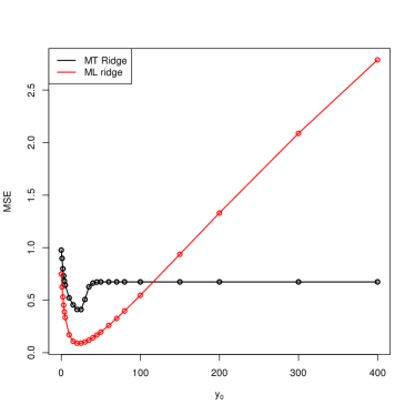
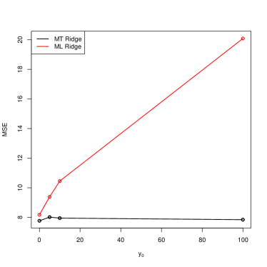
Figure 1: Mean squared errors of MT Ridge and ML Ridge for AVY setting, with $p=50$, $n=100$ and $\epsilon=0.1$ (left) and for AMR setting with $p=1600$, $n=50$ and $\epsilon=0.1$ (right).

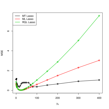
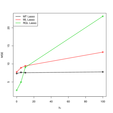
Figure 2: Mean squared errors of MT Lasso, ML Lasso and RQL Lasso for AVY setting, with $p=50$, $n=100$ and $\epsilon=0.1$ (left) and for AMR setting with $p=1600$, $n=50$ and $\epsilon=0.1$ (right).

7 Example: Right Heart Catheterization

To illustrate the proposed procedures, we analyze the rhc datset. This data set was used by Connors et al. [1996] to study the effect of Right Heart Catheterization (RHC) in critically ill patients and has been analyzed in Agostinelli et al. [2019]. A detailed description of the covariates can be found in Connors et al. [1996]. The data were downloaded from the repository at Vanderbilt University, specifically from

Ψhttp://biostat.mc.vanderbilt.edu/wiki/pub/Main/DataSets/rhc.csv

We concentrate on the data corresponding to patients with chronic obstructive pulmonary disease (COPD) as primary disease category. This leaves us with $457$ observations, for which we want to use the available variables to explain the length of hospital stay. Since the study only involves patients that have been in hospital for $2$ or more days, we define the response variable as $y=\text{ length of hospital stay}-2$, computed as discharge date minus admission date minus $2$. The matrix of covariates contains information on $57$ variables for each of the 457 patients. We assume that $y|\mathbf{x}$ follows a Poisson distribution with mean $\mu=\exp(\mathbf{x}^{\top}\boldsymbol{\beta})$ and we seek to estimate $\boldsymbol{\beta}$ and predict the length of hospital stay. We compute all the estimates using a training set composed of $75\%$ of the observations and then compute predictions and deviance residuals for the test set, composed of the rest of the observations. The training and test set were chosen at random. Figure 3 gives boxplots of the absolute deviance residuals for each method. We also give the medians of the absolute deviance residuals for each fit in Table 1.

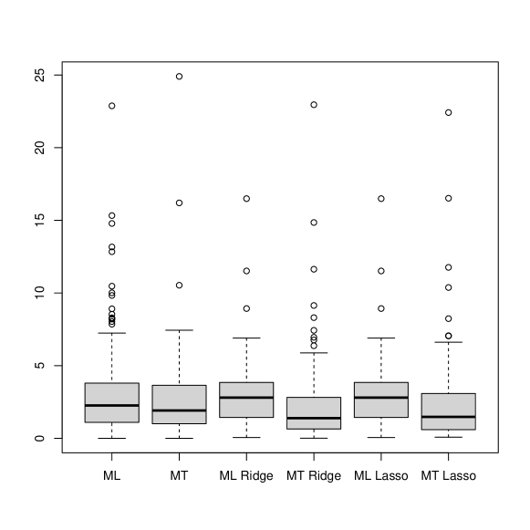
Figure 3: RHC dataset. Boxplots of absolute deviance residuals for several methods.

	ML	MT	ML Ridge	MT Ridge	ML Lasso	MT Lasso	RQL Lasso
1	2.26	1.91	2.80	1.39	2.80	1.47	59.55

Table 1: RHC datatset. Median of absolute deviance residuals for several methods.

Figure 3 and Table 1 show that MT Ridge and MT Lasso give a better prediction for the majority of the data in the test set than ML Ridge, ML Lasso and RQL Lasso. In particular, RQL Lasso gives a very bad fit for this data set so, in what follows, we exclude it from the analysis.

We next focus on outlier detection. With this aim, we generate a bootstrap sample of deviance residuals of size $B=100000$ in the following way. For $k=1,\ldots,B$, we randomly choose an index $i\in\{1,\ldots,n\}$ and we generate a response $y\sim\mathcal{P}(\mathbf{x}_{i}^{\top}\hat{\boldsymbol{\beta}})$, where $\mathbf{x}_{i}$ is the $i$-th row of the matrix of covariates and $\hat{\boldsymbol{\beta}}$ is a robust estimate (MT Lasso or MT Rigde) and we compute the corresponding deviance residual. Let $q_{1}$ and $q_{2}$ be the $1/n$ and $1-1/n$ quantiles of the bootstrap sample of deviance residuals, where $n$ is the sample size. Observations with a deviance residual smaller than $q_{1}$ or larger than $q_{2}$ will be considered outliers. For MT Lasso we obtain $q_{1}=-2.9$, $q_{2}=2.7$ and 100 outliers, that is approximately $29\%$ of the training observations while for MT Ridge we obtain $q_{1}=-2.8$ and $q_{2}=2.7$ and 105 outliers, that is aproximately $31\%$ of the training sample. Figure 4 shows the deviance residuals vs. the fitted values for MT Ridge and MT Lasso; observations with residuals outside the band determined by $q_{1}$ and $q_{2}$ are considered outliers.

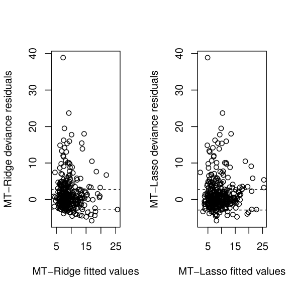
Figure 4: RHC dataset. Deviance residuals vs. fitted values for MT Ridge and MT Lasso. Broken lines correspond to $q_{1}$ and $q_{2}$.

We now compute ML Ridge and ML Lasso using only the observations with deviance residuals in the interval $(q_{1},q_{2})$. We denote these estimates ML^∗Ridge and ML^∗ Lasso respectively. Computing absolute deviance residuals for these estimators we obtain median values $1.61$ and $1.5$ respectively, similar to those obtained with MT Ridge and MT Lasso.

Finally, we take a look at the coefficient estimates. ML Lasso selects zero covariates, since all coefficient estimates equal 0 except for the intercept. Something similar happens with ML Ridge: all the coefficient estimates are almost zero (with absolute value smaller than $10^{-30}$), except for the intercept. However MT Lasso selects 15 covariates and ML^∗ Lasso selects 19. MT Ridge and ML^∗ Ridge estimates are larger than $0.0001$ for 22 and 31 coefficients respectively, as shown in Table 3.

ML Lasso ML^∗ Lasso MT Lasso (Intercept) 2.8500 -0.4100 0.0100 age 0.0000 0.0000 0.0100 raceother 0.0000 -0.0800 0.0000 ninsclasPrivate 0.0000 -0.1600 0.0000 caYes 0.0000 -0.1100 0.0000 surv2md1 0.0000 -0.8100 0.0000 aps1 0.0000 0.0000 0.0100 temp1 0.0000 0.0700 0.0600 resp1 0.0000 -0.0000 -0.0100 paco21 0.0000 -0.0000 -0.0100 ph1 0.0000 0.1000 0.0000 wblc1 0.0000 0.0000 0.0100 crea1 0.0000 0.0400 0.0000 bili1 0.0000 0.0200 0.0000 hemaYes 0.0000 0.3800 0.0000 sepsYes 0.0000 0.1200 0.0000 liverhx1 0.0000 0.0300 0.0000

Table 2: RHC dataset. Estimated coefficient by Lasso methods up to the fourth decimal digit.

ML Ridge ML^∗ Ridge MT Ridge (Intercept) 2.8464 -0.0215 0.3947 age -0.0000 0.0017 0.0068 sexMale 0.0000 0.0151 0.0002 raceother -0.0000 -0.0808 -0.0001 racewhite 0.0000 0.0061 0.0000 edu 0.0000 -0.0031 0.0001 income$25-$50k -0.0000 -0.0214 0.0000 income$>$ $50k 0.0000 0.0288 0.0000 incomeUnder $11k 0.0000 0.0213 0.0001 ninsclasMedicare 0.0000 -0.0203 -0.0001 ninsclasMedicare & Medicaid -0.0000 0.0263 0.0001 ninsclasNo insurance -0.0000 0.0352 0.0000 ninsclasPrivate 0.0000 -0.1094 -0.0001 ninsclasPrivate & Medicare -0.0000 0.0267 0.0001 das2d3pc -0.0000 -0.0017 0.0007 dnr1Yes -0.0000 0.0023 -0.0000 caNo 0.0000 0.0311 0.0001 caYes -0.0000 -0.0740 -0.0001 surv2md1 -0.0000 -0.3812 -0.0000 aps1 0.0000 0.0032 0.0054 scoma1 0.0000 0.0013 0.0024 wtkilo1 0.0000 0.0012 0.0040 temp1 -0.0000 0.0378 0.0033 meanbp1 -0.0000 -0.0015 -0.0026 resp1 -0.0000 -0.0019 -0.0024 hrt1 -0.0000 -0.0002 -0.0001 pafi1 0.0000 -0.0003 0.0012 paco21 0.0000 -0.0012 -0.0003 ph1 0.0000 0.1516 0.0005 wblc1 0.0000 0.0020 0.0041 hema1 -0.0000 -0.0014 -0.0015 sod1 -0.0000 0.0002 0.0077 pot1 0.0000 0.0026 0.0003 crea1 -0.0000 0.0326 0.0005 bili1 0.0000 0.0187 0.0007 alb1 -0.0000 -0.0320 0.0001 respYes -0.0000 -0.0010 0.0001 cardYes -0.0000 0.0103 0.0000 neuroYes 0.0000 0.1270 0.0001 gastrYes 0.0000 0.0617 -0.0001 renalYes -0.0000 -0.0658 -0.0000 metaYes -0.0000 -0.0467 -0.0000 hemaYes 0.0000 0.5874 0.0000 sepsYes 0.0000 0.1542 0.0001 cardiohx1 -0.0000 -0.0141 -0.0002 chfhx1 -0.0000 0.0352 0.0002 dementhx1 -0.0000 -0.0007 0.0001 psychhx1 0.0000 -0.0244 -0.0000 chrpulhx1 0.0000 0.0031 0.0001 renalhx1 -0.0000 -0.1116 -0.0000 liverhx1 0.0000 0.1753 -0.0000 immunhx1 -0.0000 0.0087 -0.0000 transhx1 -0.0000 0.0086 0.0001 amihx1 -0.0000 0.0569 0.0000

Table 3: RHC dataset. Estimated coefficient by Ridge methods up to the fourth decimal digit.

8 Conclusion

This paper addresses the issue of robust estimation in the context of high-dimensional covariates for generalized linear models (GLMs). To this end, we introduce penalized MT-estimators. These estimators are constructed by incorporating a penalty term into the MT-estimators defined in Valdora and Yohai [2014] and further studied in Agostinelli et al. [2019]. We focus on the elastic net penalization, though most of the results in this paper can be extended to other penalties, as far as they are locally Lipschitz. The elastic net penalty includes, as particular cases, the Ridge and the Lasso penalties

We give theoretic results regarding strong consistency, convergence rate and asymptotic normality for the general class of GLMs. We also give a numerical algorithm which allows to efficiently compute the proposed estimators.

We study the performance of the proposed estimators in finite samples by a Monte Carlo study, for the case of Poisson response. This simulation study shows the good robustness properties of the proposed estimators. We also consider a real data set in which we seek to explain and predict the length of hospital stay of patients with chronic obstructive pulmonary disease as primary disease category, using a large number of covariates. In this example, we see that both MT Lasso and MT Ridge give a better prediction for the majority of the data than their non-robust counterparts and that MT Lasso allows variable selection. We also show how both MT Lasso and MT Ridge can be used for outlier detection.

To sum up, the proposed estimators constitute useful methods for the analysis of high dimensional data, allowing to perform good predictions even in the presence of outliers, to perform robust variable selection and also to effectively detect outliers.

Appendix A Proofs

In this appendix we provide auxiliary results and detailed proofs of the results presented in Section 5. Throughout this Appendix, we assume $(y_{1},\mathbf{x}_{1}),\dots(y_{n},\mathbf{x}_{n}),$ and $(y,\mathbf{x})$ follow a GLMs with parameter $\boldsymbol{\beta}_{*}$, link function $g$ and distribution function $F$, that $\rho$ and $t$ are functions $\mathbb{R}\rightarrow\mathbb{R}$ and that $m$ is the function defined in (3). We use the notation introduced in Section 2 to 5, furthermore to simplify the notation we assume without loss of generality that $a(\phi)\equiv 1$.

A.1 Proofs of the results in Section 5

The following Lemma states the Fisher consistency of MT-estimators and has already been proved in Valdora and Yohai [2014]. We include it here for the sake of completeness.

Lemma 7 (Fisher-Consistency)

Let $L(\boldsymbol{\beta})$ be the function defined in (2) Under assumption A2, $L(\boldsymbol{\beta})$ has a unique minimum at $\boldsymbol{\beta}=\boldsymbol{\beta}_{*}$. Therefore MT-estimators are Fisher consistent.

Proof. Let $y|\mathbf{x}\sim F(\mu_{\mathbf{x}},\phi)$ and $\mu_{\mathbf{x}}=\exp(\mathbf{x}^{\top}\boldsymbol{\beta}_{*})$, then

$$\operatorname{\mathbb{E}}(\rho(t(y)-mg^{-1}(\mathbf{x}^{\top}\boldsymbol{\beta})))=\operatorname{\mathbb{E}}\left[\operatorname{\mathbb{E}}(\rho(t(y)-mg^{-1}(\mathbf{x}^{\top}\boldsymbol{\beta}))\mid\mathbf{x})\right]$$

The conditional expectation on the right is minimized in $\boldsymbol{\beta}=\boldsymbol{\beta}_{*}$ by definition of $m$, for all $\mathbf{z}$. Therefore, so is its expectation.   

The following concerns the Vapnik-Chervonenkis (VC) dimension of a class of functions; see a definition in Kosorok [2008]. The proof is similar to Lemma S.2.1 in Boente et al. [2020]; see also Lemma 4.2.2 in Smucler [2016].

Lemma 8 (VC-index)

Assume A2, B1 and B3 hold. Then the class of functions

$$\mathcal{F}=\{f:\mathbb{R}\times\mathbb{R}^{p}\rightarrow\mathbb{R},\,\,f(v,\mathbf{w})=\rho(t(v)-mg^{-1}(\beta_{0}+\mathbf{w}\boldsymbol{\beta_{1}})):\beta_{0}\in\mathbb{R},\ \boldsymbol{\beta_{1}}\in\mathbb{R}^{p}\}\ .$$

is VC-subgraph with VC-index at most $2(p+3)-1$.

Proof. Consider the set of functions

$$\mathcal{F}_{1}=\{f(v,\mathbf{w})=\beta_{0}+\mathbf{w}^{\top}\boldsymbol{\beta_{1}}:\beta_{0}\in\mathbb{R},\ \boldsymbol{\beta_{1}}\in\mathbb{R}^{p}\}\ .$$

$\mathcal{F}_{1}$ is a subset of the vector space of all affine functions in $p+1$ variables, hence e.g. by Lemma 9.6 of Kosorok [2008], $\mathcal{F}_{1}$ is VC-subgraph with VC-index at most $p+3$. Using Lemma 9.9 (viii) of Kosorok [2008] we get that

$$\mathcal{F}_{2}=\{f(v,\mathbf{w})=mg^{-1}(\beta_{0}+\mathbf{w}^{\top}\boldsymbol{\beta_{1}}):\beta_{0}\in\mathbb{R},\ \boldsymbol{\beta_{1}}\in\mathbb{R}^{p}\}$$

is also VC-subgraph with VC-index at most $p+3$ and, using item (v) of the same lemma we get that the class of functions

$$\mathcal{F}_{3}=\{f(v,\mathbf{w})=t(v)-mg^{-1}(\beta_{0}+\mathbf{w}\top\boldsymbol{\beta_{1}}):\beta_{0}\in\mathbb{R},\ \boldsymbol{\beta_{1}}\in\mathbb{R}^{p}\}$$

is VC-subgraph with at most VC-index $p+3$. Consider the functions $\rho^{+}(s)=\rho(s)\mathbb{I}_{[0,\infty)}(s)$ and $\rho^{-}(s)=\rho(s)\mathbb{I}_{(-\infty,0)}(s)$ which are monotone by B1 and B3, and $\rho(s)=\max\{\rho^{+}(s),\rho^{-}(s)\}$. Hence, by appling Lemma 9.9 (viii) and (ii) of Kosorok [2008] we have that both

$$\mathcal{F}^{+} =\{f(v,\mathbf{w})=\rho^{+}(t(v)-mg^{-1}(\beta_{0}+\mathbf{w}\top\boldsymbol{\beta_{1}})):\beta_{0}\in\mathbb{R},\ \boldsymbol{\beta_{1}}\in\mathbb{R}^{p}\}$$

$$\mathcal{F}^{-} =\{f(v,\mathbf{w})=\rho^{-}(t(v)-mg^{-1}(\beta_{0}+\mathbf{w}^{\top}\boldsymbol{\beta_{1}}))):\beta_{0}\in\mathbb{R},\ \boldsymbol{\beta_{1}}\in\mathbb{R}^{p}\}.$$

are VC-subgraph and $\mathcal{F}=\mathcal{F}^{+}\vee\mathcal{F}^{-}$ is VC-subgraph with VC-index at most $2(p+3)-1$.   

The following four lemmas have been proved in Valdora and Yohai [2014], as part of the proofs of Theorem 1 and Lemma 1. We give statements and proofs here, for the sake of completeness. Let $B(\mathbf{t},\epsilon)=\left\{\mathbf{s}\in\mathbb{R}^{p+1}/||\mathbf{s}-\mathbf{t}||\leq\epsilon\right\}$.

Lemma 9

1. Let $\mathbf{w}$, $\mathbf{t}\in\mathbb{R}^{p+1}$ be such that $\mathbf{w}^{\top}\mathbf{t}>0$, then there exist $\epsilon>0$ and $C_{\mathbf{t}}$ a compact set in $\mathbb{R}^{p+1}$ such that for all $\mathbf{s}\in B(\mathbf{t},\epsilon)$ and $\mathbf{w}\in C_{\mathbf{t}}$, $\operatorname{sign}\left(\mathbf{w}^{\top}\mathbf{t}\right)=\operatorname{sign}\left(\mathbf{w}^{\top}\mathbf{s}\right)$ and $\left|\mathbf{w}^{\top}\mathbf{s}\right|>\epsilon.$

2. If $\mathbf{x}$ is a random vector such that $\mathbb{P}(\mathbf{x}^{\top}\mathbf{t}=0)<\delta$, then the set $C_{\mathbf{t}}$ can be chosen in such a way that $P(\mathbf{x}\in C_{\mathbf{t}})>1-\delta$.

Proof.

1. Let $\varsigma$ be such that $\mathbf{w}^{\top}\mathbf{t}>\varsigma$ and $K$ be such that $||\mathbf{w}||\leq K$. Take $\epsilon=\varsigma/(2K)$ and $C_{\mathbf{t}}=\left\{\mathbf{u}\in\mathbb{R}^{p+1}:|\mathbf{u}^{\top}\mathbf{t}|\geq\varsigma,||\mathbf{u}||\leq K\right\}$.

2. Note that, since $\mathbb{P}(\mathbf{x}^{\top}\mathbf{t}=0)<\delta$, there exist $\xi$ and $\varsigma$ such that $\mathbb{P}(\mathbf{x}^{\top}\mathbf{t}\geq\varsigma)>1-\delta-\xi$. Also note that there exists $K\geq 1$ such that $\mathbb{P}(||\mathbf{x}||\leq K)>1-\xi$. Then $P\left(\left|\mathbf{x}^{\top}\mathbf{t}\right|\geq\varsigma,\|\mathbf{x}\|\leq K\right)\geq P\left(\left|\mathbf{x}^{\top}\mathbf{t}\right|\geq\varsigma\right)-P(\|\mathbf{x}\|>K)>1-\delta+\xi-\xi=1-\delta$.

 

Lemma 10

Assume A1-A5 and B1-B6. Then there exists a function $\Phi^{\ast}:\mathbb{R}\times\{-1,0,1\}\longrightarrow\mathbb{R}$ such that, for all $\mathbf{t},\mathbf{w}\in\mathbb{R}^{p+1}$, $v\in\mathbb{R}$,

$$\lim_{\zeta\rightarrow\infty}\rho(t(v)-mg^{-1}(\zeta\mathbf{w}^{\top}\mathbf{t}))=\Phi^{\ast}(v,\operatorname{sign}(\mathbf{w}^{\top}\mathbf{t}))$$ (12)

and if $\mathbf{w}^{\top}\mathbf{t}\neq 0$ there exists a neighborhood of $(\mathbf{t},\mathbf{w})$ where this convergence is uniform.

Proof. Let $m_{1}=\lim_{\mu\rightarrow\mu_{1}}m(\mu)$, $m_{2}=\lim_{\mu\rightarrow\mu_{2}}m(\mu)$ and $m_{0}=mg^{-1}(0)$, where $\mu_{1}$ and $\mu_{2}$ are the values defined in Section 2. These limits exist due to A2, though they may be $\infty$. Then (12) follows by taking

$$\Phi^{\ast}(y,j)=\left\{\begin{array}[]{l}\rho(t(v)-m_{1})\text{ if }j=-1\\ \rho(t(v)-m_{0})\text{ if }j=0\\ \rho(t(v)-m_{2})\text{ if }j=1\\ \end{array}\right.$$ (13)

$\Phi^{\ast}(v,j)$ is well defined due to B2, where, if $m_{i}=\pm\infty$ we understand $\rho(t(v)-m_{i})$ as $\lim_{m\rightarrow\pm\infty}\rho(t(v)-m)=1$ and it is continuous due to Lemma 3 in Valdora and Yohai [2014].

Let $\epsilon>0$ and $C_{\mathbf{t}}$ be those given in Lemma 9. We have that, for all $\mathbf{s}\in B(\mathbf{t},\epsilon)$ and $\mathbf{w}\in C_{\mathbf{t}}$, $\lim_{\zeta\rightarrow\infty}\rho(t(v)-mg^{-1}(\zeta\mathbf{w}^{\top}\mathbf{s}))=\rho(t(v)-m_{i})$ for $i=1$ or $2$. Using B4 and the fact that $B(\mathbf{t},\epsilon)\times C_{\mathbf{t}}$ is compact, we conclude that the convergence is uniform in $\mathbf{w}$ and $\mathbf{s}$; see for instance, Theorem 7.13 in Rudin [1976].   

Proof of Lemma 1. Note that assumption B3 together with (13) imply that $\tau\geq 0$. By assumption B7 there exists $\delta>0$ such that $\inf_{||\mathbf{t}||=1}\mathbb{P}\left(\mathbf{t}^{\top}\mathbf{x}\neq\mathbf{0}\right)=\delta$. Let $K_{1},K_{2}\in\mathbb{R}$ be such that $\mathbb{P}\left(\boldsymbol{\beta}_{*}^{\top}\mathbf{x}\in[K_{1},K_{2}]\right)>1-\delta/2$ and consider the event $V_{\mathbf{t}}=\left\{\mathbf{t}^{\top}\mathbf{x}\neq 0,\boldsymbol{\beta}_{*}^{\top}\mathbf{x}\in[K_{1},K_{2}]\right\}$.

$$\mathbb{P}(V_{\mathbf{t}})\geq\mathbb{P}(\mathbf{t}^{\top}\mathbf{x}\neq 0)-\mathbb{P}\left(\boldsymbol{\beta}_{*}^{\top}\mathbf{x}\notin[K_{1},K_{2}]\right)\geq\delta-\delta/2=\delta/2.$$

For each $i=1,2$, the function $C_{i}(\mu)=\mathbb{E}_{\mu}\left(\rho\left(t(y)-m_{i}\right)\right)-\mathbb{E}_{\mu}\left(\rho\left(t(y)-m(\mu)\right)\right)$ is positive and continuous by assumption B5. Then there exists $c_{0}>0$ such that, for each $i=1,2$, $C_{i}(\mu)\geq c_{0}$ for all $\mu\in[g^{-1}(K_{1}),g^{-1}(K_{2})]$. Denote $\mu_{\mathbf{x}}=g^{-1}\left(\boldsymbol{\beta}_{*}^{\top}\mathbf{x}\right)$. Then

$$\mathbb{E} \left(\Phi^{*}\left(y,\operatorname{sign}\left(\mathbf{t}^{\top}\mathbf{x}\right)\right)\right)-L(\boldsymbol{\beta}_{*})$$

$$\geq\mathbb{E}\left(\mathbb{E}\left(\Phi^{*}\left(y,\operatorname{sign}\left(\mathbf{t}^{\top}\mathbf{x}\right)\right)-\rho\left(t(y)-mg^{-1}\left(\boldsymbol{\beta}_{*}^{\top}\mathbf{x}\right)\right)\mid\mathbf{x}\right)\right)$$

$$=\mathbb{E}\left(\mathbb{E}_{\mu_{\mathbf{x}}}\left(\Phi^{*}\left(y,\operatorname{sign}\left(\mathbf{t}^{\top}\mathbf{x}\right)\right)-\rho\left(t(y)-m\left(\mu_{\mathbf{x}}\right)\right)\mid\mathbf{x}\right)\right)$$

$$\geq\mathbb{E}\left(C_{i}\left(\mu_{\mathbf{x}}\right)\mathbf{I}\left(\mathbf{x}\in V_{\mathbf{t}}\right)\right)\text{ for }i=1\text{ or }2\text{ since }\mathbf{t}^{\top}\mathbf{x}\neq 0\text{ for }\mathbf{x}\in V_{\mathbf{t}}$$

$$\geq c_{0}\,\mathbb{E}\left(\mathbf{I}\left(\mathbf{x}\in V_{\mathbf{t}}\right)\right)$$

$$\geq c_{0}\,\delta/2>0.$$

Since the bound is independent of $\mathbf{t}$, (10) follows.   

Lemma 11

Assume conditions A1-A5 and B1-B6 and B8. Then, for all $\mathbf{t}\in S$, there exists $\varepsilon>0$ such that

$$L(\boldsymbol{\beta}_{*})<\operatorname{\mathbb{E}}_{\boldsymbol{\beta}_{*}}\left(\mathop{\underline{\lim}}_{\zeta\rightarrow\infty}\inf_{\mathbf{s}\in B(\mathbf{t},\varepsilon)}\rho(t(y)-mg^{-1}(\zeta\mathbf{x}^{\top}\boldsymbol{s}))\right).$$ (14)

Proof. Because of B8, $\mathbb{P}(\mathbf{x}^{\top}\mathbf{t}=0)<1-\tau$ for all $\mathbf{t}\in S$. Let $C_{\mathbf{t}}$ be the compact set given in Lemma 9,then $P(C_{\mathbf{t}})>\tau$. Given $v\in\mathbb{R}$ and $\mathbf{w}\in\mathbb{R}^{p+1}$, by Lemma 10, we have

$$\mathop{\underline{\lim}}_{\zeta\rightarrow\infty}\inf_{\mathbf{s}\in B(\mathbf{t},\varepsilon)}\rho(t(v)-mg^{-1}(\zeta\mathbf{w}^{\top}\boldsymbol{s})) \leq\mathop{\lim}_{\zeta\rightarrow\infty}\rho\left(t(v)-mg^{-1}(\zeta\mathbf{w}^{\top}\mathbf{t})\right)$$

$$=\Phi^{\ast}(v,\operatorname{sign}(\mathbf{w}^{\top}\mathbf{t})).$$

Let us assume that the strict inequality holds for some point $\mathbf{w}\in C_{\mathbf{t}}$ and $v\in\mathbb{R}$, that is

$$\mathop{\underline{\lim}}_{\zeta\rightarrow\infty}\inf_{\mathbf{s}\in B(\mathbf{t},\varepsilon)}\rho(t(v)-mg^{-1}(\zeta\mathbf{w}^{\top}\boldsymbol{s})<{\small\Phi}^{\ast}(v,\operatorname{sign}(\mathbf{w}^{\top}\mathbf{t})),$$

then, there exist $\varsigma>0$, a sequence of positive numbers $\zeta_{n}\rightarrow\infty$ and a sequence $\mathbf{s}_{n}\in B(\mathbf{t},\varepsilon)$ such that

$$\rho(t(v)-mg^{-1}(\zeta_{n}\mathbf{w}^{\top}\boldsymbol{s}_{n})<{\Phi}^{\ast}(v,\operatorname{sign}(\mathbf{w}^{\top}\mathbf{t}))-\varsigma.$$ (15)

We can assume without loss of generality that $\mathbf{s}_{n}\rightarrow\mathbf{s}_{0},$ where $\mathbf{s}_{0}\in B(\mathbf{t},\varepsilon)$ and $\mathbf{w}^{\top}\mathbf{s}_{0}\neq 0$. Moreover the sign of $\mathbf{w}^{\top}\mathbf{s}_{n}$ is the same as the sign of $\mathbf{w}^{\top}\mathbf{s}_{0}$ and of $\mathbf{w}^{\top}\mathbf{t}$. By Lemma 10, we have

$$\lim_{n\rightarrow\infty}\rho(t(v)-mg^{-1}(\zeta_{n}\mathbf{w}^{\top}\boldsymbol{s}_{n})=\Phi^{\ast}(v,\operatorname{sign}(\mathbf{w}^{\top}\mathbf{s}_{0}))=\Phi^{\ast}(v,\operatorname{sign}(\mathbf{w}^{\top}\mathbf{t})).$$

contradicting (15). Then

$$\mathop{\underline{\lim}}_{\zeta\rightarrow\infty}\inf_{\mathbf{s}\in B(\mathbf{t},\varepsilon)}\rho(t(v)-mg^{-1}(\zeta\mathbf{w}^{\top}\boldsymbol{s}))=\Phi^{\ast}(v,\operatorname{sign}(\mathbf{w}^{\top}\mathbf{t})).$$

Given a set $A,$ we denote $A^{c}$ its complement. Then since $P(C_{\mathbf{t}}^{c})<1-\tau$ and $\sup\Phi^{\ast}\leq 1$, because of Lemma 10 we get

$$\operatorname{\mathbb{E}}_{\boldsymbol{\beta}_{*}}(\mathop{\underline{\lim}}_{\zeta\rightarrow\infty}\inf_{\mathbf{s}\in B(\mathbf{t},\varepsilon)}\rho(t(y)-mg^{-1}(\zeta\mathbf{x}^{\top}\boldsymbol{s})) \geq\operatorname{\mathbb{E}}_{\boldsymbol{\beta}_{*}}(\mathop{\underline{\lim}}_{\zeta\rightarrow\infty}\inf_{\mathbf{s}\in B(\mathbf{t},\varepsilon)}\rho(t(y)-mg^{-1}(\zeta\mathbf{x}^{\top}\boldsymbol{s})\mathbb{I}_{C_{\mathbf{t}}}(\mathbf{x}))$$

$$=\operatorname{\mathbb{E}}_{\boldsymbol{\beta}_{*}}(\Phi^{\ast}(y,\operatorname{sign}(\mathbf{x}^{\top}\mathbf{t}))\mathbb{I}_{C_{\mathbf{t}}}(\mathbf{x}))$$

$$=\operatorname{\mathbb{E}}_{\boldsymbol{\beta}_{*}}\left(\Phi^{\ast}(y,\operatorname{sign}(\mathbf{x}^{\top}\mathbf{t}))-{\Phi}^{\ast}(y,\operatorname{sign}(\mathbf{x}^{\top}\mathbf{t}))\mathbb{I}_{C_{\mathbf{t}}^{c}}(\mathbf{x})\right)$$

$$\geq\operatorname{\mathbb{E}}_{\boldsymbol{\beta}_{*}}(\Phi^{\ast}(y,\operatorname{sign}(\mathbf{x}^{\top}\mathbf{t})))-\mathbb{P}\left(C_{\mathbf{t}}^{c}\right)$$

$$>\operatorname{\mathbb{E}}_{\boldsymbol{\beta}_{*}}(\Phi^{\ast}(y,\operatorname{sign}(\mathbf{x}^{\top}\mathbf{t})))-\tau$$

$$\geq L(\boldsymbol{\beta}_{*})$$

This concludes the proof.    The following is a general consistency theorem valid for a large class of estimators that includes penalized MT-estimators. It has been stated and proved in Theorem S.2.1 in the Supplement to Bianco et al. [2023] for the particular case of logistic regression. However, the same proof is valid for general GLMs.

Theorem 12

Let $\widehat{\boldsymbol{\beta}}_{n}$ be an estimator defined as

$$\widehat{\boldsymbol{\beta}}_{n}=\underset{\boldsymbol{\beta}\in\mathbb{R}^{p}}{\operatorname{argmin}}\frac{1}{n}\sum_{i=1}^{n}\Phi\left(y_{i},\mathbf{x}_{i}^{\top}\boldsymbol{\beta}\right)+I_{\lambda_{n}}(\boldsymbol{\beta}),$$ (16)

where $\Phi:\mathbb{R}^{2}\longrightarrow\mathbb{R}$ and $I_{\lambda_{n}}:\mathbb{R}^{p+1}\longrightarrow\mathbb{R}$. Assume $L(\boldsymbol{\beta})=\mathbb{E}\left(\Phi(y,\mathrm{x}^{\top}\boldsymbol{\beta})\right)$ has a unique minimum at $\boldsymbol{\beta}=\boldsymbol{\beta}_{*}$ and that $I_{\lambda_{n}}\left(\boldsymbol{\beta}_{*}\right)\stackrel{{\scriptstyle\text{ a.s }}}{{\longrightarrow}}0$ when $n\rightarrow\infty$. Furthermore, assume that, for any $\epsilon>0$,

$$\inf_{\left\|\boldsymbol{\beta}-\boldsymbol{\beta}_{0}\right\|>\epsilon}L(\boldsymbol{\beta})>L\left(\boldsymbol{\beta}_{*}\right)$$ (17)

and that the following uniform Law of Large Numbers holds

$$\mathbb{P}\left(\lim_{n\rightarrow\infty}\sup_{\boldsymbol{\beta}\in\mathbb{R}^{p}}\left|\frac{1}{n}\sum_{i=1}^{n}\Phi\left(y_{i},\mathbf{x}_{i}^{\top}\boldsymbol{\beta}\right)-\mathbb{E}\left(\Phi(y,\mathbf{x}^{\top}\boldsymbol{\beta})\right)\right|=0\right)=1.$$ (18)

Then, $\widehat{\boldsymbol{\beta}}_{n}$ is strongly consistent for $\boldsymbol{\beta}_{*}$.

Proof. The proof is the same as the proof of Theorem A.2 in Bianco et al. [2023], with $L_{n}(\boldsymbol{\beta})=\frac{1}{n}\sum_{i=1}^{n}\Phi\left(y_{i},\mathbf{x}_{i}^{\top}\boldsymbol{\beta}\right),\,\,\,L(\boldsymbol{\beta})=\mathbb{E}\left(\Phi\left(y,\mathbf{x}^{\top}\boldsymbol{\beta}\right)\right)$ and $w(\mathbf{x})=1$.   

Proof of Theorem 2 . It is enough to show that the conditions in Theorem 12 hold, with $\Phi(y,\mathbf{x}^{\top}\boldsymbol{\beta})=\rho(t(y)-mg^{-1}\left(\mathbf{x}^{\top}\boldsymbol{\beta}\right))$. First note that, because of Lemma 7, $L(\boldsymbol{\beta})$ has a unique minimum at $\boldsymbol{\beta_{*}}$. Second, we prove (18) by applying Corollary 3.12 in Geer [2000]. To apply this corollary, note that $\left|\Phi(y,\mathbf{x}^{\top}\boldsymbol{\beta})\right|=\left|\rho(t(y)-mg^{-1}\left(\mathbf{x}^{\top}\boldsymbol{\beta}\right))\right|$ is uniformly bounded and that, by Lemma 8, the family

$$\mathcal{F}=\left\{f_{\boldsymbol{\beta}}(v,\mathbf{w})=\Phi(v,\mathbf{w}^{\top}\boldsymbol{\beta}),\boldsymbol{\beta}\in\mathbb{R}^{p+1}\right\}$$

is VC-subgraph with envelope $F=1$. The mentioned corollary then implies that the family $\mathcal{F}$ satisfies the Uniform Law of Large Numbers and (18) follows. It remains to prove (17) holds for all $\epsilon>0$. Assume there exists $\epsilon>0$ such that (17) does not hold. Then there exists a sequence $\left(\boldsymbol{\beta}_{n}\right)_{n}$ such that $\left\|\boldsymbol{\beta}_{n}-\boldsymbol{\beta}_{*}\right\|>\epsilon$ and $\lim_{n_{\rightarrow}\infty}L(\boldsymbol{\beta}_{n})=l\leq L\left(\boldsymbol{\beta}_{*}\right)$. Assume first $\boldsymbol{\beta}_{n}$ is bounded, then it has a subsequence $\boldsymbol{\beta}_{n_{k}}$ such that $\lim_{n_{\rightarrow}\infty}L(\boldsymbol{\beta}_{n})=L\left(\boldsymbol{\beta}_{**}\right)$ for some $\boldsymbol{\beta}_{**}$ with $\left\|\boldsymbol{\beta}_{**}-\boldsymbol{\beta}_{*}\right\|>\epsilon$. Since $L\left(\boldsymbol{\beta}_{*}\right)<L\left(\boldsymbol{\beta}_{**}\right)$ by Lemma 7 we arrive at a contradiction. This means that the sequence $\boldsymbol{\beta}_{n}$ must be unbounded. Let $\boldsymbol{\gamma}_{n}=\boldsymbol{\beta}_{n}/||\boldsymbol{\beta}_{n}||$. We can assume without loss of generality that $\lim_{n\rightarrow\infty}\boldsymbol{\gamma}_{n}=\boldsymbol{\gamma}_{*}$ with $\boldsymbol{\gamma}_{*}=1$ and that $\lim_{n\rightarrow\infty}||\boldsymbol{\beta}_{n}||$. By Lemma 11, there exists $\epsilon>0$ such that

$$L(\boldsymbol{\beta}_{*})<\operatorname{\mathbb{E}}_{\boldsymbol{\beta}_{*}}(\mathop{\underline{\lim}}_{a\rightarrow\infty}\inf_{\boldsymbol{\gamma}\in B(\boldsymbol{\gamma}_{*},\varepsilon)}\Phi(y,\mathbf{x}^{\top}a\boldsymbol{\gamma})).$$ (19)

For each $M>0$ we can choose $n_{0}\in\mathbb{N}$ such that, for all $n\geq n_{0}$, $\left|\left|\boldsymbol{\beta}_{n}\right|\right|>M$ and $\boldsymbol{\gamma}_{n}\in B(\boldsymbol{\gamma}_{*},\varepsilon)$. Then

$$\Phi(y,\mathbf{x}^{\top}\boldsymbol{\beta}_{n})=\Phi(y,M\mathbf{x}^{\top}\boldsymbol{\gamma}_{n})\geq\inf_{a>M}\inf_{\boldsymbol{\gamma}\in B(\boldsymbol{\gamma}_{*},\varepsilon)}\Phi(y,a\mathbf{x}^{\top}\boldsymbol{\gamma}).$$

$$\lim_{n\rightarrow\infty}\Phi(y,\mathbf{x}^{\top}\boldsymbol{\beta}_{n})\geq\mathop{\underline{\lim}}_{a\rightarrow\infty}\inf_{\boldsymbol{\gamma}\in B(\boldsymbol{\gamma}_{*},\varepsilon)}\Phi(y,a\mathbf{x}^{\top}\boldsymbol{\gamma})$$

By the dominated convergence theorem and (19),

$$\lim_{n\rightarrow\infty}L(\boldsymbol{\beta}_{n})=\operatorname{\mathbb{E}}\left(\lim_{n\rightarrow\infty}\Phi(y,\mathbf{x}^{\top}\boldsymbol{\beta}_{n})\right)\geq\operatorname{\mathbb{E}}\left(\mathop{\underline{\lim}}_{a\rightarrow\infty}\inf_{\boldsymbol{\gamma}\in B(\boldsymbol{\gamma}_{*},\varepsilon)}\Phi(y,a\mathbf{x}^{\top}\boldsymbol{\gamma})\right)>L(\boldsymbol{\beta_{*}}),$$

which is a contradiction. This implies (17) and the theorem follows.   

The following lemma is a direct consequence of Lemma 4.2 in v.J. Yohai [1985]. We include it here, together with its proof, for the sake of completeness.

Lemma 13

Let $\tilde{\boldsymbol{\beta}}_{n}$ be a sequence of estimators such that $\tilde{\boldsymbol{\beta}}_{n}\rightarrow\boldsymbol{\beta}_{*}$ a.s.. Suppose C1, C2 and C4 hold. Then

$$\mathop{\lim_{n\rightarrow\infty}}\mathbf{A}_{n}(\tilde{\boldsymbol{\beta}}_{n})=\mathbf{A}\quad\text{a.s.},$$

where $\mathbf{A}_{n}$ and $\mathbf{A}$ are given in (11).

Proof. First note that it is enough to prove that, for all $\epsilon>0$

$$\mathop{\overline{\lim}_{n\rightarrow\infty}}\mathbf{A}_{n}(\tilde{\boldsymbol{\beta}}_{n})<\mathbf{A}+\epsilon\qquad\text{and}\qquad\mathop{\underline{\lim}_{n\rightarrow\infty}}\mathbf{A}_{n}(\tilde{\boldsymbol{\beta}}_{n})>\mathbf{A}-\epsilon$$

Then it is enough to show that for all $\epsilon>0$ there exists $\delta>0$ such that

$$\mathop{\overline{\lim}_{n\rightarrow\infty}}\mathop{\sup_{||\boldsymbol{\beta}-\boldsymbol{\beta}_{*}||<\delta}}\mathbf{A}_{n}(\boldsymbol{\beta})<\mathbf{A}+\epsilon\qquad\text{and}\qquad\mathop{\underline{\lim}_{n\rightarrow\infty}}\mathop{\inf_{||\boldsymbol{\beta}-\boldsymbol{\beta}_{*}||<\delta}}\mathbf{A}_{n}(\boldsymbol{\beta})<\mathbf{A}-\epsilon$$ (20)

To prove the first inequality, note that, by the dominated convergence theorem and the continuity of $\mathbf{J}$, there exists $\delta$ such that

$$\operatorname{\mathbb{E}}(\mathop{\sup_{||\boldsymbol{\beta}-\boldsymbol{\beta}_{*}||<\delta}}\mathbf{J}(y,\mathbf{x},\boldsymbol{\beta}))<\operatorname{\mathbb{E}}(\mathbf{J}(y,\mathbf{x},\boldsymbol{\beta}_{*}))+\epsilon.$$

Using the Law of Large Numbers we get the first inequality in (20). The second inequality is proved similarly.   

Lemma 14

Assume conditions A1-A5, B1-B7 and C1-C4. Then,

1. $\mathop{\lim}_{\boldsymbol{\beta}\rightarrow\boldsymbol{\beta}_{*}}\operatorname{\mathbb{E}}(\mathbf{J}(y,\mathbf{x},\boldsymbol{\beta}))=\operatorname{\mathbb{E}}(\mathbf{J}(y,\mathbf{x},\boldsymbol{\beta}_{*}))$

2. Let $\eta$ be the constant given in assumption C4. Then, for all $\delta\in(0,\eta)$,

   $$\sup_{\|\boldsymbol{\beta}-\boldsymbol{\beta}_{*}\|<\delta}\frac{1}{n}\sum_{i=1}^{n}\mathbf{J}(y_{i},\mathbf{x}_{i},\boldsymbol{\beta})-\operatorname{\mathbb{E}}(\mathbf{J}(y,\mathbf{x},\boldsymbol{\beta}))\stackrel{{\scriptstyle{a.s.}}}{{\longrightarrow}}0.$$ (21)

Proof. Part (a) follows from the dominated convergence theorem and conditions C1, C2 and C4. To prove part (b) we follow the lines of the proof of Lemma 1 in Bianco and Boente [2002]. We prove the result componentwise. Fix a component of $J^{j,l}$ of $\mathbf{J}$ and $\delta\in(0,\eta)$. From Theorem 2 in Chapter 2 in Pollard [1984], it is enough to show that for all $\epsilon>0$, there exists a finite class of functions $\mathcal{F}_{\epsilon}$ such that for all $f$ in the class

$$\mathcal{F}=\left\{f_{\boldsymbol{\beta}}(v,\mathbf{w})=J^{k,l}(v,\mathbf{w},\boldsymbol{\beta}),||\boldsymbol{\beta}-\boldsymbol{\beta}_{*}||\leq\delta\right\},$$

there exist functions $f_{\epsilon}^{-}$, $f_{\epsilon}^{+}$ $\in\mathcal{F}_{\epsilon}$ such that

$$f_{\epsilon}^{-}\leq f\leq f_{\epsilon}^{+}\quad\text{ and }\quad\operatorname{\mathbb{E}}(f^{+}_{\epsilon}(y,\mathbf{x})-f^{-}_{\epsilon}(y,\mathbf{x}))<\epsilon.$$ (22)

Let $\mathcal{A}_{K}=\left\{(v,\mathbf{w})\in\mathbb{R}^{p+2}||\mathbf{w}||\leq K,|v|\leq K\right\}$, then, for all $v\in\mathbb{R},\mathbf{w}\in\mathbb{R}^{p+1}$, $\mathop{\lim}_{K\rightarrow\infty}\mathbb{I}_{\mathcal{A}_{K}^{c}}(v,\mathbf{w})=0$, so

$$\mathop{\lim}_{K\rightarrow\infty}\mathop{\sup}_{||\boldsymbol{\beta}-\boldsymbol{\beta}_{*}||\leq\delta}\left|J^{k,l}(v,\mathbf{w},\boldsymbol{\beta})\right|\mathbb{I}_{\mathcal{A}_{K}^{c}}(v,\mathbf{w})=0.$$ (23)

Because of C4 and the dominated convergence theorem, there exists $K_{0}$, such that for all $K\geq K_{0}$ and $\delta<\eta$,

$$\operatorname{\mathbb{E}}\left(\mathop{\sup}_{||\boldsymbol{\beta}-\boldsymbol{\beta}_{*}||\leq\delta}\left|J^{k,l}(y,\mathbf{x},\boldsymbol{\beta})\right|\mathbb{I}_{\mathcal{A}_{K}^{c}}(y,\mathbf{x})\right)<\epsilon/8.$$ (24)

Because of C1, C2 and Lemmas 3 and 5 in Valdora and Yohai [2014], $J^{k,l}$ is uniformly continuous in $\mathcal{A}_{K}\times\{||\boldsymbol{\beta}-\boldsymbol{\beta}_{*}||\leq\delta\}$, then there exists $\xi$ such that

$$|J^{k,l}(v_{1},\mathbf{w}_{1},\boldsymbol{\beta_{1}})-J^{k,l}(v_{2},\mathbf{w}_{2},\boldsymbol{\beta}_{2})|<\epsilon/4$$ (25)

for all $(v_{1},\mathbf{w}_{1}),(v_{2},\mathbf{w}_{2})\in\mathcal{A}_{K}$, $\boldsymbol{\beta_{1}},\boldsymbol{\beta}_{2}\in\{||\boldsymbol{\beta}-\boldsymbol{\beta}_{*}||\leq\delta\}$ such that $||\boldsymbol{\beta_{1}}-\boldsymbol{\beta}_{2}||\leq\xi$, $||\mathbf{w}_{1}-\mathbf{w}_{2}||<\xi$ and $|v_{1}-v_{2}|<\xi$. Since $\left\{||\boldsymbol{\beta}-\boldsymbol{\beta}_{*}||\leq\delta\right\}$ is compact, there exist $B_{1},\dots,B_{N}$ balls with radius smaller than $\xi$ and centers at certain points $\boldsymbol{\beta}_{1},\dots,\boldsymbol{\beta}_{N}\in\{||\boldsymbol{\beta}-\boldsymbol{\beta}_{*}||\leq\delta\}$ such that $\left\{||\boldsymbol{\beta}-\boldsymbol{\beta}_{*}||\leq\delta\right\}\subset\bigcup_{i=1}^{N}B_{i}$. The class $\mathcal{F}_{\epsilon}$ is then the class of functions

$$f^{\pm}_{\epsilon,i}(v,\mathbf{w})=J^{k,l}(v,\mathbf{w},\boldsymbol{\beta}_{i})\pm\left(\frac{\epsilon}{4}+2\mathop{\sup}_{||\boldsymbol{\beta}-\boldsymbol{\beta}_{*}||\leq\delta}\left|J^{k,l}(v,\mathbf{w},\boldsymbol{\beta})\right|\mathbb{I}_{\mathcal{A}_{K}^{c}}(v,\mathbf{w})\right),$$

for $i\in 1,\dots,N$. To show the first inequality in (22), let $f_{\boldsymbol{\beta}}(v,\mathbf{w})=J^{k,l}(v,\mathbf{w},\boldsymbol{\beta})\in\mathcal{F}$. If $(v,\mathbf{w})\in\mathcal{A}_{K}$, then there exists $i_{0}\in\{1,\ldots,N\}$ such that $||\boldsymbol{\beta}-\boldsymbol{\beta}_{i_{0}}||\leq\xi$ and

$$|J^{k,l}(v,\mathbf{w},\boldsymbol{\beta})-J^{k,l}(v,\mathbf{w},\boldsymbol{\beta}_{i_{0}})|<\epsilon/4.$$

Then

$$f^{-}_{\epsilon,i_{0}}(v,\mathbf{w})=J^{k,l}(v,\mathbf{w},\boldsymbol{\beta}_{i_{0}})-\epsilon/4<J^{k,l}(v,\mathbf{w},\boldsymbol{\beta})<J^{k,l}(v,\mathbf{w},\boldsymbol{\beta}_{i_{0}})+\epsilon/4=f^{+}_{\epsilon,i_{0}}(v,\mathbf{w}).$$

If $(v,\mathbf{w})\in\mathcal{A}_{K}^{c}$, because of the triangular inequality,

$$|J^{k,l}(v,\mathbf{w},\boldsymbol{\beta})-J^{k,l}(v,\mathbf{w},\boldsymbol{\beta}_{i_{0}})|\leq 2\sup_{||\boldsymbol{\beta}-\boldsymbol{\beta}_{*}||<\delta}|J^{k,l}(v,\mathbf{w},\boldsymbol{\beta})|.$$

Then

$$J^{k,l}(v,\mathbf{w},\boldsymbol{\beta})\leq J^{k,l}(v,\mathbf{w},\boldsymbol{\beta}_{i_{0}})+2\mathop{\sup}_{||\boldsymbol{\beta}-\boldsymbol{\beta}_{*}||\leq\delta}\left|J^{k,l}(v,\mathbf{w},\boldsymbol{\beta})\right|\leq f^{+}_{\epsilon,i_{0}}(v,\mathbf{w})$$

and

$$J^{k,l}(v,\mathbf{w},\boldsymbol{\beta})\geq J^{k,l}(v,\mathbf{w},\boldsymbol{\beta}_{i_{0}})-2\mathop{\sup}_{||\boldsymbol{\beta}-\boldsymbol{\beta}_{*}||\leq\delta}\left|J^{k,l}(v,\mathbf{w},\boldsymbol{\beta})\right|\geq f^{-}_{\epsilon,i_{0}}(v,\mathbf{w}).$$

To show the second inequality in (22), note that, by definition of $f^{\pm}_{\epsilon,i}$ and (24),

$$\operatorname{\mathbb{E}}(f^{+}_{\epsilon,i_{0}}(y,\mathbf{x})-f^{-}_{\epsilon,i_{0}}(y,\mathbf{x}))=\frac{\epsilon}{2}+4\operatorname{\mathbb{E}}\left(\mathop{\sup}_{||\boldsymbol{\beta}-\boldsymbol{\beta}_{*}||\leq\delta}\left|J^{k,l}(y,\mathbf{x},\boldsymbol{\beta})\right|\mathbb{I}_{\mathcal{A}_{K}^{c}}(y,\mathbf{x})\right)<\epsilon.$$

 

Proof of Theorem 3. Let $W_{n}(\boldsymbol{\beta})=L_{n}(\boldsymbol{\beta})+\lambda_{n}P_{\alpha}(\boldsymbol{\beta})$ and $\mathbf{A}$ and $\mathbf{A}_{n}(\boldsymbol{\beta})$ as defined in (11). Because of the definition of $\hat{\boldsymbol{\beta}}_{n}$, $W_{n}(\hat{\boldsymbol{\beta}}_{n})-W_{n}(\boldsymbol{\beta}_{*})\leq 0$. Using a Taylor expansion of $L_{n}(\hat{\boldsymbol{\beta}}_{n})$ about $\boldsymbol{\beta}_{*}$, we obtain that for a certain point $\boldsymbol{\xi}_{n}=\boldsymbol{\beta}_{*}+\tau_{n}(\hat{\boldsymbol{\beta}}_{n}-\boldsymbol{\beta}_{*})$ with $\tau_{n}\in[0,1]$,

$$0 \geq\frac{1}{n}\sum_{i=1}^{n}\ \boldsymbol{\Psi}(y_{i},\mathbf{x}_{i},\boldsymbol{\beta}_{*})^{\top}(\hat{\boldsymbol{\beta}}_{n}-\boldsymbol{\beta}_{*})+(\hat{\boldsymbol{\beta}}_{n}-\boldsymbol{\beta}_{*})^{\top}\mathbf{A}_{n}(\boldsymbol{\xi}_{n})(\hat{\boldsymbol{\beta}}_{n}-\boldsymbol{\beta}_{*})$$

$$+\lambda_{n}P_{\alpha}(\hat{\boldsymbol{\beta}}_{n})-\lambda_{n}P_{\alpha}(\boldsymbol{\beta}_{*})$$

$$=\frac{1}{n}\sum_{i=1}^{n}\ \boldsymbol{\Psi}(y_{i},\mathbf{x}_{i},\boldsymbol{\beta}_{*})^{\top}(\hat{\boldsymbol{\beta}}_{n}-\boldsymbol{\beta}_{*})+(\hat{\boldsymbol{\beta}}_{n}-\boldsymbol{\beta}_{*})^{\top}(\mathbf{A}_{n}(\boldsymbol{\xi}_{n})-\mathbf{A})(\hat{\boldsymbol{\beta}}_{n}-\boldsymbol{\beta}_{*})$$

$$+(\hat{\boldsymbol{\beta}}_{n}-\boldsymbol{\beta}_{*})^{\top}\mathbf{A}(\hat{\boldsymbol{\beta}}_{n}-\boldsymbol{\beta}_{*})+\lambda_{n}P_{\alpha}(\hat{\boldsymbol{\beta}}_{n})-\lambda_{n}P_{\alpha}(\boldsymbol{\beta}_{*})$$

$$\geq\frac{1}{n}\sum_{i=1}^{n}\boldsymbol{\Psi}(y_{i},\mathbf{x}_{i},\boldsymbol{\beta}_{*})^{\top}(\hat{\boldsymbol{\beta}}_{n}-\boldsymbol{\beta}_{*})+(\hat{\boldsymbol{\beta}}_{n}-\boldsymbol{\beta}_{*})^{\top}(\mathbf{A}_{n}(\boldsymbol{\xi}_{n})-\mathbf{A})(\hat{\boldsymbol{\beta}}_{n}-\boldsymbol{\beta}_{*})$$

$$+\zeta_{1}||\hat{\boldsymbol{\beta}}_{n}-\boldsymbol{\beta}_{*}||^{2}+\lambda_{n}\{P_{\alpha}(\hat{\boldsymbol{\beta}}_{n})-P_{\alpha}(\boldsymbol{\beta}_{*})\},$$

where $\zeta_{1}$ is the smallest eigenvalue of $\mathbf{A}$ which we know is positive by C4. Since the third term in the above sum is positive, the sum of the other three terms must be negative and therefore equal to minus its absolute value. Applying the triangle inequality we get that the complete sum is

$$\geq-\frac{1}{n}\sum_{i=1}^{n}||\boldsymbol{\Psi}(y_{i},\mathbf{x}_{i},\boldsymbol{\beta}_{*})||||\hat{\boldsymbol{\beta}}_{n}-\boldsymbol{\beta}_{*}||-||\hat{\boldsymbol{\beta}}_{n}-\boldsymbol{\beta}_{*}||^{2}||\mathbf{A}_{n}(\boldsymbol{\xi}_{n})-\mathbf{A}||$$

$$+\zeta_{1}||\hat{\boldsymbol{\beta}}_{n}-\boldsymbol{\beta}_{*}||^{2}-\lambda_{n}|P_{\alpha}(\hat{\boldsymbol{\beta}}_{n})-P_{\alpha}(\boldsymbol{\beta}_{*})|\ .$$

Let $\epsilon>0$. To bound the first term note that the Central Limit Theorem and Lemma 7 imply that

$$\sqrt{n}\frac{1}{n}\sum_{i=1}^{n}\boldsymbol{\Psi}(y_{i},\mathbf{x}_{i},\boldsymbol{\beta}_{*})=O_{P}(1)$$

Therefore there exists a constant $M_{1}$ such that, for all $n$, $P(\mathcal{C}_{n})>1-\varepsilon/4$, where $\mathcal{C}_{n}=\left\{\left\|\sqrt{n}\frac{1}{n}\sum_{i=1}^{n}\boldsymbol{\Psi}(y_{i},\mathbf{x}_{i},\boldsymbol{\beta}_{*})\right\|<M_{1}\right\}$.

To bound the second term, note that, since $\hat{\boldsymbol{\beta}}_{n}\stackrel{{\scriptstyle p}}{{\longrightarrow}}\boldsymbol{\beta}_{*}$, from Lemma 14, we have that $\mathbf{A}_{n}(\hat{\boldsymbol{\beta}}_{n})\stackrel{{\scriptstyle p}}{{\longrightarrow}}\mathbf{A}$, so there exists $n_{1}$ such that for every $n\geq n_{1},P(\mathcal{B}_{n})>1-\varepsilon/4$, where $\mathcal{B}_{n}=\left\{\left\|\mathbf{A}_{n}(\boldsymbol{\xi}_{n})-\mathbf{A}\right\|<\zeta_{1}/2\right\}$.

Finally, to bound the third term, note that the function $P_{\alpha}(.)$ is Lipschitz with constant $K$ independent of $\alpha$, in a neighbourhood of $\boldsymbol{\beta}_{*}$ and define the event

$$\mathcal{D}_{n}=\left\{\mathop{\sup_{\alpha\in[0,1]}}|P_{\alpha}(\hat{\boldsymbol{\beta}}_{n})-P_{\alpha}(\boldsymbol{\beta}_{*})|\leq K\left\|\hat{\boldsymbol{\beta}}_{n}-\boldsymbol{\beta}_{*}\right\|\right\}.$$

Then, there exists $n_{2}\in\mathbb{N}$ such that for $n\geq n_{2}$, $P(\mathcal{D}_{n})\geq 1-\epsilon/2$. Hence, for $n\geq\max\left\{n_{1},n_{2}\right\}$ we have that $P(\mathcal{B}_{n}\cap\mathcal{C}_{n}\cap\mathcal{D}_{n})>1-\epsilon$. Besides, in $\mathcal{B}_{n}\cap\mathcal{C}_{n}\cap\mathcal{D}_{n}$ we have that

$$0\geq-\left\|\hat{\boldsymbol{\beta}}_{n}-\boldsymbol{\beta}_{*}\right\|\frac{1}{\sqrt{n}}M_{1}+\frac{\zeta_{1}}{2}\left\|\hat{\boldsymbol{\beta}}_{n}-\boldsymbol{\beta}_{*}\right\|^{2}-K\lambda_{n}\left\|\hat{\boldsymbol{\beta}}_{n}-\boldsymbol{\beta}_{*}\right\|$$

which implies

$$\left\|\hat{\boldsymbol{\beta}}_{n}-\boldsymbol{\beta}_{*}\right\|\leq 2\left(\lambda_{n}+\frac{1}{\sqrt{n}}\right)\frac{M_{1}+K}{\zeta_{1}}.$$

Hence, $\left\|\hat{\boldsymbol{\beta}}_{n}-\boldsymbol{\beta}_{*}\right\|=O_{P}(\lambda_{n}+1/\sqrt{n})$, which completes the proof.   

A.2 Proofs of the results in Section 5

We now turn to the proof of the asymptotic normality of the proposed estimators. To derive the proof of Theorem 4 we will need two lemmas.

Lemma 15

Assume C1, C2 nd C4. For each $\mathbf{w}\in\mathbb{R}^{p+1}$, define

$$R_{1}(\mathbf{w})=\mathbf{w}_{0}^{\top}\mathbf{w}+\frac{1}{2}\mathbf{w}^{\top}\mathbf{A}\mathbf{w}$$

where $\mathbf{w}_{0}\sim N_{p+1}(\mathbf{0},\mathbf{B})$ with $\mathbf{B}$ given in (11). Furthermore, let $R_{n,1}(\mathbf{w})$ be

$$R_{n,1}(\mathbf{w}) =\sum_{i=1}^{n}\left\{\rho\left(t(y_{i})-mg^{-1}\left(\mathbf{x}_{i}^{\top}\left[\boldsymbol{\beta}_{*}+\frac{\mathbf{w}}{\sqrt{n}}\right]\right)\right)-\rho\left(t(y_{i})-mg^{-1}\left(\mathbf{x}_{i}^{\top}\boldsymbol{\beta}_{*}\right)\right)\right\}.$$

Then, the process $R_{n,1}$ converges in distribution to $R_{1}$.

Proof. The proof is similar to the proof of Lemma A.7 in Bianco et al. [2019]. According to Theorem 2.3 in Kim and Pollard [1990], it is enough to prove that

• For any $\mathbf{w}_{1},\cdots,\mathbf{w}_{s}$ we have

  $$(R_{n,1}(\mathbf{w}_{1}),\cdots,R_{n,1}(\mathbf{w}_{s}))\stackrel{{\scriptstyle d}}{{\longrightarrow}}(R_{1}(\mathbf{w}_{1}),\cdots,R_{1}(\mathbf{w}_{s}))$$

• Given $\epsilon>0,\eta>0$ and $M<\infty$ there exists $\delta>0$ such that

  $$\limsup_{n\rightarrow\infty}P^{*}\left(\sup_{\|\mathbf{u}\|\leq M,\|\mathbf{v}\|\leq M\atop\|\mathbf{u}-\mathbf{v}\|<\delta}\left|R_{n,1}(\mathbf{u})-R_{n,1}(\mathbf{v})\right|>\epsilon\right)<\eta$$

  where $P^{*}$ stands for outer probability.

First note that it is enough to consider $s=1$ since for any other $s$ the proof follows similarly using the Cramer-Wald device. Hence, we fix $\mathbf{w}\in\mathbb{R}^{p+1}$. A Taylor expansion of $R_{n,1}$ around $\mathbf{w}=\mathbf{0}$ yields

$$R_{n,1}(\mathbf{w})=\sqrt{n}\mathbf{w}^{\top}\nabla L_{n}(\boldsymbol{\beta}_{*})+\frac{1}{2}\mathbf{w}^{\top}\mathbf{A}_{n}(\tilde{\boldsymbol{\beta}}_{\mathbf{w}})\mathbf{w},$$

with $\mathbf{A}_{n}(\boldsymbol{\beta})$ as defined in (11) and $\tilde{\boldsymbol{\beta}}_{\mathbf{w}}=\boldsymbol{\beta}_{*}+\tau_{n}\mathbf{w}/\sqrt{n}$ with $\tau_{n}\in[0,1]$. Note that $\nabla L_{n}(\boldsymbol{\beta})=\frac{1}{n}\sum_{i=1}^{n}\mathbf{\Psi}(y_{i},\mathbf{x}_{i},\boldsymbol{\beta})$. The Multivariate Central Limit Theorem and Lemma 7 entail that $\sqrt{n}\nabla L_{n}(\boldsymbol{\beta}_{*})\stackrel{{\scriptstyle d}}{{\longrightarrow}}N_{p+1}(\mathbf{0},\mathbf{B})$. On the other hand, Lemma 13 implies that $\mathbf{A}_{n}(\tilde{\boldsymbol{\beta}}_{\mathbf{w}})\stackrel{{\scriptstyle p}}{{\longrightarrow}}\mathbf{A}$, so using Slutsky’s Theorem we obtain that $R_{n,1}\stackrel{{\scriptstyle d}}{{\longrightarrow}}\mathbf{w}_{0}^{\top}\mathbf{w}+\frac{1}{2}\mathbf{w}^{\top}\mathbf{A}\mathbf{w}$, concluding the proof of (a).

To derive (b), we perform a first order Taylor expansion of $R_{n,1}(\mathbf{u})$ and $R_{n,1}(\mathbf{v})$ around $0$ obtaining

$$R_{n,1}(\mathbf{u})-R_{n,1}(\mathbf{v})=\sqrt{n}\nabla L_{n}(\boldsymbol{\beta}_{*})^{\top}(\mathbf{u}-\mathbf{v})+\frac{1}{2}\mathbf{u}^{\top}\mathbf{A}_{n}(\tilde{\boldsymbol{\beta}}_{\mathbf{u}})\mathbf{u}-\frac{1}{2}\mathbf{v}^{\top}\mathbf{A}_{n}(\tilde{\boldsymbol{\beta}}_{\mathbf{v}})\mathbf{v}$$

where $\tilde{\boldsymbol{\beta}}_{\mathbf{v}}=\boldsymbol{\beta}_{*}+{\tau_{\mathbf{v},n}\mathbf{v}}/{\sqrt{n}}$ and $\tilde{\boldsymbol{\beta}}_{\mathbf{u}}=\boldsymbol{\beta}_{*}+{\tau_{\mathbf{u},n}\mathbf{u}}/{\sqrt{n}}$ with $\tau_{\mathbf{v},n},\tau_{\mathbf{u},n}\in[0,1]$. Noting that $\sqrt{n}\nabla L_{n}(\boldsymbol{\beta}_{*})^{\top}(\mathbf{u}-\mathbf{v})\leq O_{P}(1)\|\mathbf{u}-\mathbf{v}\|$ and

$$\mathbf{u}^{\top}\mathbf{A}_{n}(\tilde{\boldsymbol{\beta}}_{\mathbf{u}})\mathbf{u}-\mathbf{v}^{\top}\mathbf{A}_{n}(\tilde{\boldsymbol{\beta}}_{\mathbf{v}})\mathbf{v} =\mathbf{u}^{\top}\mathbf{A}_{n}(\tilde{\boldsymbol{\beta}}_{\mathbf{u}})\mathbf{u}-\mathbf{u}^{\top}\mathbf{A}_{n}(\tilde{\boldsymbol{\beta}}_{\mathbf{v}})\mathbf{u}+\mathbf{u}^{\top}\mathbf{A}_{n}(\tilde{\boldsymbol{\beta}}_{\mathbf{v}})\mathbf{u}$$

$$-\mathbf{u}^{\top}\mathbf{A}_{n}(\tilde{\boldsymbol{\beta}}_{\mathbf{v}})\mathbf{v}+\mathbf{u}^{\top}\mathbf{A}_{n}(\tilde{\boldsymbol{\beta}}_{\mathbf{v}})\mathbf{v}-\mathbf{v}^{\top}\mathbf{A}_{n}(\tilde{\boldsymbol{\beta}}_{\mathbf{v}})\mathbf{v}$$

we obtain that, if $\|\mathbf{u}\|,\|\mathbf{v}\|\leq M$,

$$\left|R_{n,1}(\mathbf{u})-R_{n,2}(\mathbf{v})\right|\leq O_{p}(1)\|\mathbf{u}-\mathbf{v}\|+M^{2}\left\|\mathbf{A}_{n}(\tilde{\boldsymbol{\beta}}_{\mathbf{u}})-\mathbf{A}_{n}(\tilde{\boldsymbol{\beta}}_{\mathbf{v}})\right\|$$

$$+2\|\mathbf{u}-\mathbf{v}\|M\left\|\mathbf{A}_{n}(\tilde{\boldsymbol{\beta}}_{\mathbf{v}})\right\|$$

where $\|\mathbf{C}\|$ stands for the Frobenius norm if $\mathbf{C}$ is a matrix. Lemma 14 entails that $\mathbf{A}_{n}(\tilde{\boldsymbol{\beta}}_{\mathbf{u}})-\mathbf{A}_{n}(\tilde{\boldsymbol{\beta}}_{\mathbf{v}})\stackrel{{\scriptstyle p}}{{\longrightarrow}}0$ and $\mathbf{A}_{n}(\tilde{\boldsymbol{\beta}}_{\mathbf{v}})\stackrel{{\scriptstyle p}}{{\longrightarrow}}\mathbf{A}$, uniformly over all $\left\{\mathbf{u},\mathbf{v}\in\mathbb{R}^{p+1}:\max\{\|\mathbf{u}\|,\|\mathbf{v}\|\}\leq M\right\}$ and $(\mathrm{b})$ follows, concluding the proof.    In the next Lemma and in Theorem 4 $\lambda_{n}$ is allowed to be random.

Lemma 16

Let $P_{\alpha}$ be as in (8) and assume $\sqrt{n}\lambda_{n}=O_{P}(1)$. Let $\mathbf{w}=(w_{0},\mathbf{w}_{1})\in\mathbb{R}^{p+1}$ and

$$R_{n,2}(\mathbf{w})=n\lambda_{n}\left\{P_{\alpha}\left(\boldsymbol{\beta}_{*}+\frac{\mathbf{w}}{\sqrt{n}}\right)-P_{\alpha}(\boldsymbol{\beta}_{*})\right\}.$$

Then, the process $R_{n,2}$ is equicontinuous, i.e., for any $\epsilon>0,\eta>0$ and $M<\infty$ there exists $\delta>0$ such that

$$\limsup_{n\rightarrow\infty}P^{*}\left(\sup_{\|\mathbf{u}||\leq M,\|\mathbf{v}\|\leq M\atop\|\mathbf{u}-\mathbf{v}\|<\delta}\left|R_{n,2}(\mathbf{u})-R_{n,2}(\mathbf{v})\right|>\epsilon\right)<\eta.$$

Proof. Since the function $P_{\alpha}(.)$ is Lipschitz with constant $K$ independent of $\alpha$, in a neighbourhood of $\boldsymbol{\beta}_{*}$, there exists $M$ such that, if $||\mathbf{u}||<M$ and $||\mathbf{v}||<M$,

$$\left|R_{n,2}(\mathbf{u})-R_{n,2}(\mathbf{v})\right|=n\lambda_{n}\left|P_{\alpha}\left(\boldsymbol{\beta}_{*}+\frac{\mathbf{u}}{\sqrt{n}}\right)-P_{\alpha}\left(\boldsymbol{\beta}_{*}+\frac{\mathbf{v}}{\sqrt{n}}\right)\right|\leq K\sqrt{n}\lambda_{n}\left\|\mathbf{u}-\mathbf{v}\right\|.$$

Since $\sqrt{n}\lambda_{n}=O_{P}(1)$, there exists $C$ such that $P(\sqrt{n}\lambda_{n}\geq C)<\eta$, then, if $||\mathbf{u}-\mathbf{v}||<\epsilon/(CK)$, $||\mathbf{u}||<M$ and $||\mathbf{v}||<M$,

$$P^{*}\left(\left|R_{n,2}(\mathbf{u})-R_{n,2}(\mathbf{v})\right|>\epsilon\right)\leq P\left(\sqrt{n}\lambda n>\frac{\epsilon}{K||\mathbf{u}-\mathbf{v}||}\right)\leq P\left(\sqrt{n}\lambda n>M\right)<\eta.$$

The result follows taking $\delta=\epsilon/(CK)$.   

Proof of Theorem 4. The proof is similar to the proof of Theorem 5.3 in Bianco et al. [2019]. Let $R_{n}(\mathbf{w})=R_{n,1}(\mathbf{w})+R_{n,2}(\mathbf{w})$, with $R_{n,1}(\mathbf{w})$ and $R_{n,2}(\mathbf{w})$ defined as in Lemmas 15 and 16 respectively and note that $\arg\min_{\mathbf{w}}R_{n}(\mathbf{w})=\sqrt{n}(\hat{\boldsymbol{\beta}}_{n}-\boldsymbol{\beta}_{*})$. So what we need to prove is that

$$\operatorname{argmin}_{\mathbf{w}}R_{n}(\mathbf{w})\rightarrow\operatorname{argmin}_{\mathbf{w}}R(\mathbf{w}).$$

We will use Theorem 2.7 in Kim and Pollard [1990] with $t_{n}=-\sqrt{n}(\hat{\boldsymbol{\beta}}_{n}-\boldsymbol{\beta}_{*})$, $Z=-R(\mathbf{w})$ and $Z_{n}=R_{n}$. Condition (iii) is verified since $R_{n}(\sqrt{n}(\hat{\boldsymbol{\beta}}_{n}-\boldsymbol{\beta}_{*}))\leq\inf_{\mathbf{t}}R_{n}(\mathbf{t})$ while condition (ii) follows from Theorem 3. To verify (i) we need to prove that $R_{n}(\mathbf{w})\stackrel{{\scriptstyle d}}{{\rightarrow}}R(\mathbf{w})$. As explained in the proof of Lemma 15, it is enough to show that

• For any $\mathbf{w}_{1},\cdots,\mathbf{w}_{s}$ we have $(R_{n}(\mathbf{w}_{1}),\cdots,R_{n}(\mathbf{w}_{s}))\stackrel{{\scriptstyle d}}{{\longrightarrow}}(R(\mathbf{w}_{1}),\cdots,R(\mathbf{w}_{s}))$.

• Given $\epsilon>0,\eta>0$ and $M<\infty$ there exists $\delta>0$ such that

  $$\limsup_{n\rightarrow\infty}P^{*}\left(\sup_{\|\mathbf{u}\|\leq M,\|\mathbf{v}\|\leq M\atop\|\mathbf{u}-\mathbf{v}\|<\delta}\left|R_{n}(\mathbf{u})-R_{n}(\mathbf{v})\right|>\epsilon\right)<\eta$$

  where $P^{*}$ stands for outer probability.

First note that (b) follows easily from Lemmas 15 and 16. To prove (a), recall from the proof of Lemma 15 that it is enough to consider the case $s=1$ and fix $\mathbf{w}\in\mathbb{R}^{p+1}$. We already know $R_{n,1}(\mathbf{w})\stackrel{{\scriptstyle d}}{{\longrightarrow}}\mathbf{w}^{\top}\mathbf{w}_{0}+\frac{1}{2}\mathbf{w}^{\top}\mathbf{A}\mathbf{w}$, so we only have to study the convergence of $R_{n,2}(\mathbf{w})$.

Note that $R_{n,2}(\mathbf{w})=R_{n,2,1}(\mathbf{w})+R_{n,2,2}(\mathbf{w})$ where $\mathbf{w}=(w_{0},w_{1},\dots,w_{p})$ and

$$R_{n,2,1}(\mathbf{w}) =n\lambda_{n}\frac{1-\alpha}{2}\left\{\sum_{\ell=1}^{p}\left(\beta_{*,\ell}+\frac{w_{\ell}}{\sqrt{n}}\right)^{2}-(\beta_{*,\ell})^{2}\right\}$$

$$R_{n,2,2}(\mathbf{w}) =n\lambda_{n}\alpha\left\{\sum_{\ell=1}^{p}\left|\beta_{*,\ell}+\frac{w_{\ell}}{\sqrt{n}}\right|-\left|\beta_{*,\ell}\right|\right\}$$

$$R_{n,2,1}(\mathbf{w})=n\lambda_{n}\frac{1-\alpha}{2}\sum_{\ell=1}^{p}\left\{2\beta_{*,\ell}\frac{w_{\ell}}{\sqrt{n}}+\frac{w_{\ell}^{2}}{n}\right\}=\sqrt{n}\lambda_{n}(1-\alpha)\sum_{\ell=1}^{p}\left\{\beta_{*,\ell}w_{\ell}+\frac{w_{\ell}^{2}}{2\sqrt{n}}\right\}$$

For each $\ell=1,\dots,p$, if $\beta_{*,\ell}>0$ and $n$ is large enough, then $\beta_{*,\ell}+\frac{w_{\ell}}{\sqrt{n}}>0$ as well, and the $\ell$-th term of $R_{n,2,2}(\mathbf{w})$ is $\sqrt{n}\lambda_{n}\alpha w_{\ell}$. If $\beta_{*,\ell}<0$ and $n$ is large enough, then the $\ell$-th term of $R_{n,2,2}(\mathbf{w})$ is $-\sqrt{n}\lambda_{n}\alpha{w_{\ell}}$, while, if $\beta_{*,\ell}=0$, the $\ell$-th term in $R_{n,2,2}(\mathbf{w})$ is $\sqrt{n}\lambda_{n}\alpha{|w_{\ell}|}$. So we have that

$$R_{n,2,2}(\mathbf{w})=\sqrt{n}\lambda_{n}\alpha\sum_{\ell=1}^{p}w_{\ell}\operatorname{sign}(\beta_{*,\ell})\mathbb{I}_{\{\beta_{*,\ell}\neq 0\}}+\left|w_{\ell}\right|\mathbb{I}_{\{{\beta_{*,\ell}=0}\}}\ .$$

And then,

$$R_{n,2,1}(\mathbf{w})\stackrel{{\scriptstyle p}}{{\longrightarrow}} b(1-\alpha)\sum_{\ell=1}^{p}\beta_{*,\ell}w_{\ell}$$

$$R_{n,2,2}(\mathbf{w})\stackrel{{\scriptstyle p}}{{\longrightarrow}} b\alpha\sum_{\ell=1}^{p}\left\{w_{\ell}\operatorname{sign}(\beta_{*,\ell})\mathbb{I}_{\left\{\beta_{*,\ell}\neq 0\right\}}+|w_{\ell}|\mathbb{I}_{\left\{{\beta_{*,\ell}=0}\right\}}\right\}.$$

Therefore, $R_{n,2}(\mathbf{w})\stackrel{{\scriptstyle p}}{{\longrightarrow}}b\mathbf{w}^{\top}\mathbf{q}(\mathbf{w})$ and the result follows from Slutzky’s lemma.   

Proof of Theorem 6. Let

$$R_{n,1}(\mathbf{w}) =\frac{1}{n\lambda_{n}^{2}}\sum_{i=1}^{n}\left\{\rho(t(y_{i})-mg^{-1}(\mathbf{x}_{i}^{\top}(\boldsymbol{\beta}_{*}+\lambda_{n}\mathbf{w})))-\rho(t(y_{i})-mg^{-1}(\mathbf{x}_{i}^{\top}\boldsymbol{\beta}_{*}))\right\}$$

$$R_{n,2}(\mathbf{w}) =\frac{1}{\lambda_{n}}\left\{P_{\alpha}(\boldsymbol{\beta}_{*}+\lambda_{n}\mathbf{w})-P_{\alpha}(\boldsymbol{\beta}_{*})\right\}$$

and $R_{n}(\mathbf{w})=R_{n,1}(\mathbf{w})+R_{n,2}(\mathbf{w})$.

Note that $\arg\min_{\mathbf{w}}R_{n}(\mathbf{w})=(1/\lambda_{n})(\hat{\boldsymbol{\beta}}_{n}-\boldsymbol{\beta}_{*})$. As in the proof of Theorem 4, we begin by showing that given $\epsilon>0,\eta>0$ and $M<\infty$ there exists $\delta>0$ such that

$$\limsup_{n\rightarrow\infty}P^{*}\left(\sup_{\|\mathbf{u}\|\leq M,\|\mathbf{v}\|\leq M\atop\|\mathbf{u}-\mathbf{v}\|<\delta}\left|R_{n,l}(\mathbf{u})-R_{n,l}(\mathbf{v})\right|>\epsilon\right)<\eta\text{ for }l=1,2.$$ (26)

For $l=2$ (26) follows from the fact that $P_{\alpha}$ is locally Lipschitz.

To prove (26) for $l=1$, we use Taylor expansions of $R_{n,1}(\mathbf{u})$ and $R_{n,1}(\mathbf{v})$ around $\boldsymbol{\beta}_{*}$ and we get

$$R_{n,1}(\mathbf{u})-R_{n,1}(\mathbf{v})=\frac{1}{\lambda_{n}\sqrt{n}}\sqrt{n}\nabla L_{n}(\boldsymbol{\beta}_{*})^{\top}(\mathbf{u}-\mathbf{v})+\frac{1}{2}\mathbf{u}^{\top}\mathbf{A}_{n}(\tilde{\boldsymbol{\beta}}_{\mathbf{u}})\mathbf{u}-\frac{1}{2}\mathbf{v}^{\top}\mathbf{A}_{n}(\tilde{\boldsymbol{\beta}}_{\mathbf{v}})\mathbf{v}$$

where $\tilde{\boldsymbol{\beta}}_{\mathbf{u}}$ and $\tilde{\boldsymbol{\beta}}_{\mathbf{v}}$ are intermediate points defined as

$$\tilde{\boldsymbol{\beta}}_{\mathbf{u}}=\boldsymbol{\beta}_{*}+\lambda_{n}\tau_{\mathbf{u},n}\mathbf{u}\quad\text{ and }\quad\tilde{\boldsymbol{\beta}}_{\mathbf{v}}=\boldsymbol{\beta}_{*}+\lambda_{n}\tau_{\mathbf{v},n}\mathbf{v}$$

with $\tau_{\mathbf{u},n},\tau_{\mathbf{v},n}\in[0,1]$. As in the proof of Lemma 15, using that $\sqrt{n}\nabla L_{n}(\boldsymbol{\beta}_{*})\stackrel{{\scriptstyle d}}{{\longrightarrow}}N_{p+1}(\mathbf{0},\mathbf{B})$, we conclude that $\sqrt{n}\nabla L_{n}(\boldsymbol{\beta}_{*})^{\top}(\mathbf{u}-\mathbf{v})\leq O_{P}(1)\|\mathbf{u}-\mathbf{v}\|.$ On the other hand,

$$\mathbf{u}^{\top}\mathbf{A}_{n}(\tilde{\boldsymbol{\beta}}_{\mathbf{u}})\mathbf{u}-\mathbf{v}^{\top}\mathbf{A}_{n}(\tilde{\boldsymbol{\beta}}_{\mathbf{v}})\mathbf{v} =\mathbf{u}^{\top}\mathbf{A}_{n}(\tilde{\boldsymbol{\beta}}_{\mathbf{u}})\mathbf{u}-\mathbf{u}^{\top}\mathbf{A}_{n}(\tilde{\boldsymbol{\beta}}_{\mathbf{v}})\mathbf{u}+\mathbf{u}^{\top}\mathbf{A}_{n}(\tilde{\boldsymbol{\beta}}_{\mathbf{v}})\mathbf{u}$$

$$-\mathbf{u}^{\top}\mathbf{A}_{n}(\tilde{\boldsymbol{\beta}}_{\mathbf{v}})\mathbf{v}+\mathbf{u}^{\top}\mathbf{A}_{n}(\tilde{\boldsymbol{\beta}}_{\mathbf{v}})\mathbf{v}-\mathbf{v}^{\top}\mathbf{A}_{n}(\tilde{\boldsymbol{\beta}}_{\mathbf{v}})\mathbf{v}$$

so, if $\|\mathbf{u}\|,\|\mathbf{v}\|\leq M$

$$\left|R_{n,1}(\mathbf{u})-R_{n,1}(\mathbf{v})\right|\leq \frac{1}{\lambda_{n}\sqrt{n}}O_{p}(1){\|\mathbf{u}-\mathbf{v}\|}+M^{2}\left\|\mathbf{A}_{n}(\tilde{\boldsymbol{\beta}}_{\mathbf{u}})-\mathbf{A}_{n}(\tilde{\boldsymbol{\beta}}_{\mathbf{v}})\right\|$$

$$+2\|\mathbf{u}-\mathbf{v}\|M\left\|\mathbf{A}_{n}(\tilde{\boldsymbol{\beta}}_{\mathbf{v}})\right\|.$$

Using that $\lambda_{n}\sqrt{n}\rightarrow\infty$ and that $\mathbf{A}_{n}(\tilde{\boldsymbol{\beta}}_{\mathbf{u}})-\mathbf{A}_{n}(\tilde{\boldsymbol{\beta}}_{\mathbf{v}})\stackrel{{\scriptstyle p}}{{\longrightarrow}}0$ and $\mathbf{A}_{n}(\tilde{\boldsymbol{\beta}}_{\mathbf{v}})\stackrel{{\scriptstyle p}}{{\longrightarrow}}\mathbf{A}$ uniformly over $\left\{\mathbf{u},\mathbf{v}\in\mathbb{R}^{p}:\max\{\|\mathbf{u}\|,\|\mathbf{v}\|\}\leq M\right\}$ by Lemma 14, we get that (26) holds for $\ell=1$. It remains to see that given $\mathbf{w}_{1},\ldots,\mathbf{w}_{s}\in\mathbb{R}^{p+1}$ we have $(R_{n}(\mathbf{w}_{1}),\ldots,R_{n}(\mathbf{w}_{s}))\stackrel{{\scriptstyle d}}{{\longrightarrow}}(R(\mathbf{w}_{1}),\ldots,R(\mathbf{w}_{s}))$, where $R(\mathbf{w})=(1/2)\mathbf{w}^{\top}\mathbf{A}\mathbf{w}+\mathbf{w}^{\top}\mathbf{q}(\mathbf{w})$. As in the proof of Theorem 4, it is enough to show the result when $s=1$. Fix $\mathbf{w}\in\mathbb{R}^{p+1}$. Using again a Taylor expansion of order one, we obtain

$$R_{n,1}(\mathbf{w})=\frac{1}{\lambda_{n}\sqrt{n}}\sqrt{n}\nabla L_{n}(\boldsymbol{\beta}_{*})^{\top}\mathbf{z}+\frac{1}{2}\mathbf{z}^{\top}\mathbf{A}_{n}(\tilde{\boldsymbol{\beta}}_{\mathbf{w}})\mathbf{w}$$ (27)

where $\tilde{\boldsymbol{\beta}}_{\mathbf{w}}=\boldsymbol{\beta}_{*}+\lambda_{n}\tau_{n}\mathbf{w}$, with $\tau_{n}\in[0,1]$. Since

$$\sqrt{n}\nabla L_{n}(\boldsymbol{\beta}_{*})\stackrel{{\scriptstyle d}}{{\longrightarrow}}N_{p+1}(\mathbf{0},\mathbf{B}),$$

The fact that $\lambda_{n}\sqrt{n}\rightarrow\infty$, implies that

$$\frac{1}{\lambda_{n}\sqrt{n}}\sqrt{n}\nabla L_{n}(\boldsymbol{\beta}_{*})^{\top}\mathbf{w}\stackrel{{\scriptstyle p}}{{\longrightarrow}}0.$$

The second term in (27) converges to $(1/2)\mathbf{w}^{\top}\mathbf{A}\mathbf{w}$ in probability by Lemma 14. This proves

$$R_{n,1}(\mathbf{w})\stackrel{{\scriptstyle p}}{{\longrightarrow}}(1/2)\mathbf{w}^{\top}\mathbf{A}\mathbf{w}.$$

We now show $R_{n,2}(\mathbf{w})\stackrel{{\scriptstyle p}}{{\longrightarrow}}\mathbf{w}^{\top}\mathbf{q}(\mathbf{w})$. First note that

$$R_{n,2}(\mathbf{w})=\frac{1}{\lambda_{n}}\sum_{\ell=1}^{p}\frac{1-\alpha}{2}\left(2\beta_{*,\ell}\lambda_{n}w_{\ell}+\lambda_{n}^{2}w_{\ell}^{2})+\alpha(|\beta_{*,\ell}+\lambda_{n}w_{\ell}|-|\beta_{*,\ell}|\right).$$

Note that, for $\ell>0$ if $n$ is large enough, then $\beta_{*,\ell}+\lambda_{n}w_{\ell}$ has the same sign as $\beta_{*,\ell}$, then, as in the proof of Theorem 4, we get

$$R_{n,2}(\mathbf{w}) =\sum_{\ell=1}^{p}\frac{1-\alpha}{2}\left(2\beta_{*,\ell}w_{\ell}+\lambda_{n}w_{\ell}^{2}\right)+\alpha\left(w_{\ell}\operatorname{sign}(\beta_{*,\ell})\mathbb{I}_{\{\beta_{*,\ell}\neq 0\}}+\left|w_{\ell}\right|\mathbb{I}_{{\{\beta_{*,\ell}=0\}}}\right)$$

$$\stackrel{{\scriptstyle p}}{{\rightarrow}}b\mathbf{w}^{\top}\mathbf{q}(\mathbf{w}).$$

 

Appendix B Computational details and algorithm

We introduce an Iteratively Re-Weighted Least Square (IRWLS) algorithm in Subsection B.1 while in subsection B.2 we discuss how to obtain feasible starting values.

B.1 Iteratively Re-Weighted Least Square algorithm

An IRWLS procedure to compute the MT-estimator is described in Agostinelli et al. [2019], where we show that the solution to the minimization of (4) can be approximated by the following

$$\min_{\boldsymbol{\beta}}\sum_{i=1}^{n}\rho(t(y_{i})-s(\mathbf{x}_{i}^{\top}\boldsymbol{\beta}^{k})-s^{\prime}(\mathbf{x}_{i}^{\top}\boldsymbol{\beta}^{k})\mathbf{x}_{i}^{\top}(\boldsymbol{\beta}-\boldsymbol{\beta}^{k}),$$ (28)

where $s(\mathbf{x}_{i}^{\top}\boldsymbol{\beta}^{k})=mg^{-1}(\mathbf{x}_{i}^{\top}\boldsymbol{\beta}^{k})$.

Since the Elastic Net penalty is not differentiable, we wish to keep the minimization problem instead of replacing it by the estimating equations. The iterative procedure developed in Agostinelli et al. [2019] is based on the estimating equations. However, the same iterative method can be written in the following way

$$\min_{\boldsymbol{\beta}}\sum_{i=1}^{n}(t(y_{i})-s(\mathbf{x}_{i}^{\top}\boldsymbol{\beta}^{k})-s^{\prime}(\mathbf{x}_{i}^{\top}\boldsymbol{\beta}^{k})\mathbf{x}_{i}^{\top}(\boldsymbol{\beta}-\boldsymbol{\beta}^{k}))^{2}w_{i}^{\ast}(\mathbf{x}_{i}^{\top}\boldsymbol{\beta}^{k})$$ (29)

where $w_{i}^{\ast}(v)=\psi(t(y_{i})-s(v))/(t(y_{i})-s(v))$ and $\psi=\rho^{\prime}$. In fact, the estimating equations corresponding to problem (29) are

$$\sum_{i=1}^{n}(t(y_{i})-s(\mathbf{x}_{i}^{\top}\boldsymbol{\beta}^{k})-s^{\prime}(\mathbf{x}_{i}^{\top}\boldsymbol{\beta}^{k})\mathbf{x}_{i}^{\top}(\boldsymbol{\beta}-\boldsymbol{\beta}^{k}))w_{i}^{\ast}(\mathbf{x}_{i}^{\top}\boldsymbol{\beta}^{k})s^{\prime}(\mathbf{x}_{i}^{\top}\boldsymbol{\beta}^{k})\mathbf{x}_{i}=\mathbf{0}.$$ (30)

The IRWLS introduced in Agostinelli et al. [2019] to solve the equations above is the following. If the solution on step $k$ is $\boldsymbol{\beta}^{k}$, the solution on step $k+1$ is given by

$$\boldsymbol{\beta}^{k+1}=\boldsymbol{\beta}^{k}+(\mathbf{X}^{\top}\mathbf{W}^{2}(\mathbf{X}\boldsymbol{\beta}^{k})^{\top}\mathbf{W}^{\ast}(\mathbf{X}\boldsymbol{\beta}^{k})\mathbf{X})^{-1}\mathbf{X}^{\top}\mathbf{W}(\mathbf{X}\boldsymbol{\beta}^{k})\mathbf{W}^{\ast}(\mathbf{X}\boldsymbol{\beta}^{k})(\mathbf{T}-\mathbf{s}(\mathbf{X}\boldsymbol{\beta}^{k}))$$ (31)

where $\mathbf{X}$ is the $n\times(p+1)$ matrix whose $i$-th row is $\mathbf{x}_{i}$, $\mathbf{W}$ is a diagonal matrix whose elements are $s^{\prime}(\mathbf{x}_{i}^{\top}\boldsymbol{\beta}^{k})\mathbf{x}_{i}^{\top}\boldsymbol{\beta}^{k}$ and $\mathbf{W}^{\ast}$ is a diagonal matrix of robust weights $(w_{1}^{\ast},\ldots,w_{n}^{\ast})$ as defined below equation (29). Now we turn to the problem of solving the penalized optimization problem

$$\hat{\boldsymbol{\beta}}=\arg\min_{\boldsymbol{\beta}}\sum_{i=1}^{n}\rho(t(y_{i})-mg^{-1}(\mathbf{x}_{i}^{\top}\boldsymbol{\beta}))+\lambda P_{\alpha}(\boldsymbol{\beta}).$$

At each step of an IRWLS algorithm we can approximate our optimization problem by

$$\boldsymbol{\beta}^{k+1}=\arg\min_{\boldsymbol{\beta}}\frac{1}{2n}\sum_{i=1}^{n}(t(y_{i})-s(\mathbf{x}_{i}^{\top}\boldsymbol{\beta}^{k})-s^{\prime}(\mathbf{x}_{i}^{\top}\boldsymbol{\beta}^{k})\mathbf{x}_{i}^{\top}(\boldsymbol{\beta}-\boldsymbol{\beta}^{k}))^{2}w_{i}^{\ast}(\mathbf{x}_{i}^{\top}\boldsymbol{\beta}^{k})+\lambda P_{\alpha}(\boldsymbol{\beta})$$ (32)

which is a form of weighted Elastic Net with weights evaluated at a previous step $k$. This problem can be written as

$$\boldsymbol{\beta}^{k+1}=\arg\min_{\boldsymbol{\beta}}\frac{1}{2n}\sum_{i=1}^{n}(z_{i}^{k}-\mathbf{v}_{i}^{k\top}(\boldsymbol{\beta}-\boldsymbol{\beta}^{k}))^{2}+\lambda P_{\alpha}(\boldsymbol{\beta})$$ (33)

with $z_{i}^{k}=(t(y_{i})-s(\mathbf{x}_{i}^{\top}\boldsymbol{\beta}^{k}))\sqrt{w_{i}^{\ast}(\mathbf{x}_{i}^{\top}\boldsymbol{\beta}^{k})}$ and $\mathbf{v}_{i}^{k}=s^{\prime}(\mathbf{x}_{i}^{\top}\boldsymbol{\beta}^{k})\mathbf{x}_{i}\sqrt{w_{i}^{\ast}(\mathbf{x}_{i}^{\top}\boldsymbol{\beta}^{k})}$. Solutions to (33) can be obtained with several algorithms depending on $\alpha$ and on the dimension of the problem. Here we follow the approach in Friedman et al. [2007] which is specialized to the GLMs case in Friedman et al. [2010] using a coordinate descendent algorithm. At step $k$ we can define $\hat{z}_{i}^{k(j)}=\beta_{0}^{k}+\sum_{l\neq j}v_{il}\beta_{l}^{k}$ as the fitted value excluding the contribution from $x_{ij}$, and $z_{i}^{k}-\hat{z}_{i}^{k(j)}$ the partial residual for fitting $\beta_{j}$. Hence, as explained in Friedman et al. [2010], an update for $\beta_{j}$ can be obtained as

$$\beta_{j}^{k+1}=\frac{S\left(\frac{1}{n}\sum_{i=1}^{n}v_{ij}(z_{i}^{k}-\hat{z}_{i}^{k(j)}),\lambda\alpha\right)}{\frac{1}{n}\sum_{i=1}^{n}v_{ij}^{2}+\lambda(1-\alpha)}\qquad j=1,\ldots,p.$$ (34)

where $S(z,\gamma)=\operatorname{sign}(z)(|z|-\gamma)_{+}$ is the soft-thresholding operator, while for $j=0$,

$$\beta_{0}^{k+1}=\frac{1}{n}\sum_{i=1}^{n}(z_{i}^{k}-\hat{z}_{i}^{k(0)})$$ (35)

where $\hat{z}_{i}^{k(0)}=\sum_{l}v_{il}\beta_{l}^{k}$. In the special case $\alpha=0$ we have the Ridge penalty and instead of the coordinate descent algorithm we can solve (33) directly to obtain the Ridge normal equations

$$\beta_{0}^{k+1} =\bar{z}^{k}-\bar{\mathbf{v}}^{k\top}\boldsymbol{\beta}^{k+1}$$

$$\boldsymbol{\beta_{1}}^{k+1} =(\mathbf{V}^{k\top}\mathbf{V}^{k}+\lambda\mathbf{I})^{-1}\mathbf{V}^{k\top}(\mathbf{z}^{k}-\beta_{0}^{k+1}\mathbf{1}_{n})$$

where $\boldsymbol{\beta_{1}}^{\top}=(\beta_{1},\ldots,\beta_{p})$, $\mathbf{V}^{k}$ is the matrix with rows $\mathbf{v}_{i}^{k}$, $\mathbf{z}^{k}=(z_{1}^{k},\ldots,z_{n}^{k})^{\top}$, $\bar{\mathbf{v}}^{k}$ is the vector of the means of the columns of $\mathbf{V}^{k}$ and $\bar{z}^{k}$ is the mean of $\mathbf{z}^{k}$.

On the other hand, if $\alpha=1$, we have the Lasso penalty and (33) can also be solved with a weighted Lasso algorithm based on least angle regression as done in Alfons et al. [2013] and Smucler and Yohai [2017]. This was implemented using the function fastLasso from package robustHD, see Alfons [2019].

B.2 Procedure for obtaining a robust initial estimate

In our penalized version of MT-estimators we consider redescending $\rho$-functions and hence the goal function $\hat{L}_{n}(\boldsymbol{\beta})$ might have several local minima. As a consequence, it might happen that the IRWLS algorithm converges to a solution of the estimating equations that is not a solution of the optimization problem. In practice, to avoid this, one must begin the iterative algorithm at an initial estimator which is a very good approximation of the absolute minimum of $\hat{L}_{n}(\boldsymbol{\beta})$. If $p$ is small, an approximate solution may be obtained by the subsampling method which consists in computing a finite set $A$ of candidate solutions and then replace the minimization over $\mathbb{R}^{p+1}$ by a minimization over $A$. The set $A$ is obtained by randomly drawing subsamples of size $p+1$ and computing the maximum likelihood estimator based on the subsample. Assume the original sample contains a proportion $\epsilon$ of outliers, then the probability of having at least one subsample free of outliers is $1-(1-(1-\epsilon)^{p})^{N}$ where $N$ is the number of subsamples drawn. So, for a given probability $\alpha$ such that $1-(1-(1-\epsilon)^{p})^{N}>\alpha$ we need

$$N>\frac{\log(\alpha)}{\log(1-(1-\varepsilon)^{p})}\underline{\sim}\left|\frac{\log(\alpha)}{(1-\varepsilon)^{p}}\right|.$$

This makes the algorithm based on subsampling infeasible for large $p$. We instead propose an adaptation of the procedure in Agostinelli et al. [2019] which is a deterministic algorithm.

Consider a random sample following a generalized linear model. The following procedure computes an approximation of $\boldsymbol{\beta}_{*}$ which will be used as an initial estimator in the IRWLS algorithm for the estimating equation describe in Subsection B.1. The procedure has two stages. Stage 1 aims at finding a highly robust but possibly inefficient estimate and stage 2 aims at increasing its efficiency.

Stage 1. In this stage, the idea is to find a robust, but possibly inefficient, estimate of $\boldsymbol{\beta}_{*}$ by an iterative procedure. In each iteration $k\geq 1$ we get

$$\hat{\boldsymbol{\beta}}^{(k)}=\arg\min_{\boldsymbol{\beta}\in A_{k}}\hat{L}_{n}(\boldsymbol{\beta}).$$ (36)

In the first iteration ($k=1$) the set $A_{1}$ is constructed as follows. We begin by computing the penalized LST estimate $\hat{\boldsymbol{\beta}}_{LS}^{(1)}$ with the complete sample and the principal sensitivity components [Peña and Yohai, 1999] obtained as follows. We define the fitted values $\hat{\boldsymbol{\mu}}^{(1)}=g^{-1}(\mathbf{X}\hat{\boldsymbol{\beta}}^{(1)})$ and for each index $j$ the fitted values $\hat{\boldsymbol{\mu}}_{(j)}^{(1)}=g^{-1}(\mathbf{X}\hat{\boldsymbol{\beta}}_{LS(j)}^{(1)})$ obtained by computing the penalized LST estimate $\hat{\boldsymbol{\beta}}_{LS(j)}^{(1)}$ with the sample without using observation with $j$ index. We compute the sensitivity vector $\mathbf{r}_{(j)}=\hat{\mathbf{t}}-\hat{\mathbf{t}}_{(j)}$ which is the difference between the predicted value $\hat{\mathbf{t}}=m(\hat{\boldsymbol{\mu}}^{(1)})$ based on the complete sample and $\hat{\mathbf{t}}_{(j)}=m(\hat{\boldsymbol{\mu}}_{(j)}^{(1)})$ based on the sample without the observation with $j$ index. The sensitivity matrix $\mathbf{R}$ is built from the sensitivity vectors $\mathbf{r}_{(1)},\ldots,\mathbf{r}_{(n)}$. We obtain the direction $\mathbf{v}_{1}$ in which the projections of the sensitivity vectors is largest, i.e.,

$$\mathbf{v}_{1}=\mbox{argmax}_{||\mathbf{v}||=1}\sum_{j=1}^{n}\left(\mathbf{v}^{\top}\mathbf{r}_{(j)}\right)^{2}$$

and $\mathbf{z}_{1}=\mathbf{R}\mathbf{v}_{1}$ where the largest entries in $\mathbf{z}_{1}$ correspond to the largest terms in the sum $\sum_{j=1}^{n}\left(\mathbf{v}^{\top}\mathbf{r}_{(j)}\right)^{2}$, which in turn correspond to the observations that have the largest projected sensitivity in the direction $\mathbf{v}_{1}$. Recursively we compute $\mathbf{v}_{i},$ $2\leq i\leq n$ as the solution of

$$\mathbf{v}_{i} =\arg\max_{||\mathbf{v}||=1}\sum_{j=1}^{n}\left(\mathbf{v}^{\top}\mathbf{r}_{(j)}\right)^{2}$$

$$\text{ subject to }\mathbf{v}_{i}\mathbf{v}_{j}=0\text{ for all }1\leq j<i$$

and the corresponding principal sensitivity components $\mathbf{z}_{i}=\mathbf{R}\mathbf{v}_{i}$. Large entries are considered potential outliers. For each principal sensitivity component $\mathbf{z}_{i}$ we compute three estimates by the penalized LST method. The first eliminating the half of the observations corresponding to the smallest entries in $\mathbf{z}_{i}$, the second eliminating the half corresponding to the largest entries in $\mathbf{z}_{i}$ and the third eliminating the half corresponding to the largest absolute values. To these $3p$ initial candidates we add the penalized LST estimate computed using the complete sample, obtaining a set of $3p+1$ elements. Once we have $A_{1}$ we obtain $\hat{\boldsymbol{\beta}}^{(1)}$ by minimizing $\hat{L}_{n}(\boldsymbol{\beta})$ over the elements of $A_{1}$.

Suppose now that we are on stage $k$. Let $0<\alpha<0.5$ be a trimming constant, in all our applications we set $\alpha=0.05$. Then, for $k>1$, we first delete the observations $(i=1,\cdots,n)$ such that $y_{i}>F_{\hat{\mu}_{i}^{(k-1)}}^{-1}(1-\alpha/2)$ or $y_{i}<F_{\hat{\mu}^{(k-1)}_{i}}^{-1}(\alpha/2)$ and, with the remaining observations, we re-compute the penalized LST estimator $\hat{\boldsymbol{\beta}}_{LS}^{(k)}$ and the principal sensitivity components. Let us remark that, for the computation of $\hat{\boldsymbol{\beta}}_{LS}^{(k)}$ we have deleted the observations that have large residuals, since $\hat{\boldsymbol{\mu}}^{(k-1)}$ are the fitted values obtained using $\hat{\boldsymbol{\beta}}_{LS}^{(k-1)}$. In this way, while candidates on the first step of the iteration are protected from high leverage outliers, candidate $\hat{\boldsymbol{\beta}}_{LS}^{(k)}$ is protected from low leverage outliers, which may not be extreme entries of the $\mathbf{z}_{i}$.

The set $A_{k}$ will contain $\hat{\boldsymbol{\beta}}_{LS}^{(k)}$, $\hat{\boldsymbol{\beta}}^{(k-1)}$ and the $3p$ penalized LST estimates computed deleting extreme values according to the principal sensitivity components as in the first iteration. $\hat{\boldsymbol{\beta}}^{(k)}$ is the element of $A_{k}$ minimizing $\hat{L}_{n}(\boldsymbol{\beta})$.

The iterations will continue until $\hat{\boldsymbol{\beta}}^{(k)}\approx\hat{\boldsymbol{\beta}}^{(k-1)}$. Let $\tilde{\boldsymbol{\beta}}^{(1)}$ be the final estimate obtained at this stage.

Stage 2. We first delete the observations $y_{i}$ ($i=1,\cdots,n$) such that $y_{i}>F_{\tilde{\mu}_{i}^{(1)}}^{-1}(1-\alpha/2)$ or $y_{i}<F_{\tilde{\mu}_{i}^{(1)}}^{-1}(\alpha/2)$, where $\tilde{\boldsymbol{\mu}}^{(1)}=g^{-1}\left(\mathbf{X}\tilde{\boldsymbol{\beta}}^{(1)}\right)$ and compute the penalized LST estimate $\tilde{\boldsymbol{\beta}}^{(2)}$ with the reduced sample. Then for each of the deleted observations we check whether $y_{i}>F_{\tilde{\mu}_{i}^{(2)}}^{-1}(1-\alpha/2)$ or $y_{i}<F_{\tilde{\mu}_{i}^{(2)}}^{-1}(\alpha/2)$, where $\tilde{\boldsymbol{\mu}}^{(2)}=g^{-1}\left(\mathbf{X}\tilde{\boldsymbol{\beta}}^{(2)}\right)$. Observations which are not within these bounds are finally eliminated and those which are, are restored to the sample. With the resulting set of observations we compute the penalized LST estimate $\tilde{\boldsymbol{\beta}}$ which is our proposal as a starting value for solving the estimating equations of the MT-estimates.

B.3 Asymptotic variance

Let $\eta=\mathbf{x}^{\top}\boldsymbol{\beta}$, $\dot{m}$, $\dot{(g^{-1})}$ and $\dot{\psi}$ be the derivatives with respect to their arguments and $z(y;\eta,\phi)=(t(y)-mg^{-1}(\eta))/\sqrt{a(\phi)}$.

$$\Psi(y,\mathbf{x},\boldsymbol{\beta}) =\frac{\partial}{\partial\eta}\rho(z(y;\eta,\phi))\nabla_{\boldsymbol{\beta}}\eta$$

$$=\psi(z(y;\eta,\phi))\dot{m}(g^{-1}(\eta))\dot{(g^{-1})}(\eta)a(\phi)^{-1/2}\mathbf{x}$$

$$=\psi(z(y;\eta,\phi))K_{1}(\eta)a(\phi)^{-1/2}\mathbf{x}$$

where we let $K_{1}(\eta)=\dot{m}(g^{-1}(\eta))\dot{(g^{-1})}(\eta)$. Hence

$$\mathbf{B}(\boldsymbol{\beta}) =\operatorname{\mathbb{E}}(\Psi(y,\mathbf{x},\boldsymbol{\beta})\Psi(y,\mathbf{x},\boldsymbol{\beta})^{\top})$$

$$=\operatorname{\mathbb{V}ar}\left(\psi\left(\frac{t(y)-mg^{-1}(\eta)}{\sqrt{a(\phi)}}\right)\right)K_{1}(\eta)^{2}a(\phi)^{-1}\mathbf{x}\mathbf{x}^{\top}$$

$$=B(\eta,\phi)K_{1}^{2}(\eta)a(\phi)^{-1}\mathbf{x}\mathbf{x}^{\top}$$

and since

$$\frac{\partial}{\partial\eta}K_{1}(\eta)=\ddot{m}(g^{-1})\dot{(g^{-1})}+\dot{m}(g^{-1})\ddot{(g^{-1})}=K_{2}(\eta)$$

we have

$$\mathbf{J}(y,\mathbf{x},\boldsymbol{\beta}) =\nabla\Psi(y,\mathbf{x},\boldsymbol{\beta})$$

$$=\frac{\partial}{\partial\eta}\psi\left(\frac{t(y)-mg^{-1}(\eta)}{\sqrt{a(\phi)}}\right)K_{1}(\eta)a(\phi)^{-1/2}\mathbf{x}\mathbf{x}^{\top}$$

$$+\psi(z(y;\eta,\phi))\frac{\partial}{\partial\eta}K_{1}(\eta)a(\phi)^{-1/2}\mathbf{x}\mathbf{x}^{\top}$$

$$=\dot{\psi}(z(y;\eta,\phi))K_{1}^{2}(\eta)a(\phi)^{-1}\mathbf{x}\mathbf{x}^{\top}$$

$$+\psi(z(y;\eta,\phi))K_{2}(\eta)a(\phi)^{-1/2}\mathbf{x}\mathbf{x}^{\top}$$

$$=\left[\dot{\psi}(z(y;\eta,\phi))a(\phi)^{-1/2}K_{1}^{2}(\eta)+\psi(z(y;\eta,\phi))K_{2}(\eta)\right]a(\phi)^{-1/2}\mathbf{x}\mathbf{x}^{\top}$$

we have that

$$\mathbf{A}(\boldsymbol{\beta}) =\operatorname{\mathbb{E}}(\mathbf{J}(y,\mathbf{x},\boldsymbol{\beta}))$$

$$=\left[\operatorname{\mathbb{E}}(\dot{\psi}(z(y;\eta,\phi)))a(\phi)^{-1/2}K_{1}^{2}(\eta)+\operatorname{\mathbb{E}}(\psi(z(y;\eta,\phi)))K_{2}(\eta)\right]a(\phi)^{-1/2}\mathbf{x}\mathbf{x}^{\top}$$

$$=\left[A_{1}(\eta,\phi)K_{1}^{2}(\eta)+A_{2}(\eta,\phi)K_{2}(\eta)\right]a(\phi)^{-1/2}\mathbf{x}\mathbf{x}^{\top}$$

So that, the asymptotic variance is given by

$$\mathbf{A}^{-1}(\boldsymbol{\beta})\mathbf{B}(\boldsymbol{\beta})\mathbf{A}^{-1}(\boldsymbol{\beta})=B(\eta,\phi)K_{1}^{2}(\eta)\left[A_{1}(\eta,\phi)K_{1}^{2}(\eta)+A_{2}(\eta,\phi)K_{2}(\eta)\right]^{-2}(\mathbf{x}\mathbf{x}^{\top})^{-1}$$

Appendix C Monte Carlo results

In this Section we report full results for simulation settings AVY and AMR together with the results of a third setting namely AVY2 which is similar to “model 2” considered in Agostinelli et al. [2019]. The difference with AVY described in Section 6 is in the value of parameters, which in AVY2 are given by $\boldsymbol{\beta}_{*}=2\mathbf{e}_{1}+\mathbf{e}_{2}$. All the figures are in the Supplementary Material.

C.1 False Negative and False Positive for Lasso Methods

In Tables 4 to 6 we report a summary of the performance of Lasso methods for variable selection for the AMR setting. These tables are similar to Table 1 in Avella-Medina and Ronchetti [2018]. For each measure, we give the median over 100 simulations and its median absolute deviation in parentheses. Size is the number of selected variables in the final model, $\#FN$ is the number of parameters that are incorrectly estimated as $0$, $\#FP$ is the number of parameters that are zero but their estimates are not. Tables 7 to 9 give the selected value of the penalty parameter, the BIC and the degrees of freedom for this value.

	$p=100$		$\nu=0$			$\nu=5$			$\nu=10$			$\nu=100$
$n$	$\varepsilon$	Method	Size	$\#FN$	$\#FP$	Size	$\#FN$	$\#FP$	Size	$\#FN$	$\#FP$	Size	$\#FN$	$\#FP$
50	0.05	MT	1	3	0	1.03	2.97	0.03	1	3	0	1	3	0
			(0)	(0)	(0)	(0.3)	(0.3)	(0.3)	(0)	(0)	(0)	(0)	(0)	(0)
		ML	13.39	0	12.39	21.01	0.11	20.01	22.57	0.49	21.57	14.64	2.23	13.64
			(6.3)	(0)	(6.3)	(11.16)	(0.35)	(11.16)	(12.93)	(0.61)	(12.93)	(11.19)	(0.92)	(11.19)
		RQL	12.31	0	11.31	13.45	0.02	12.45	13.71	0.02	12.71	13.82	0.06	12.82
			(3.66)	(0)	(3.66)	(4.39)	(0.14)	(4.39)	(5.07)	(0.14)	(5.07)	(5.43)	(0.28)	(5.43)
	0.1	MT	1	3	0	1.02	2.98	0.02	1	3	0	1	3	0
			(0)	(0)	(0)	(0.2)	(0.2)	(0.2)	(0)	(0)	(0)	(0)	(0)	(0)
		ML	12.02	0.05	11.02	21.24	0.23	20.24	20	1.05	19	7.16	2.64	6.16
			(5.2)	(0.26)	(5.2)	(12)	(0.47)	(12)	(14.54)	(0.97)	(14.54)	(8.03)	(0.59)	(8.03)
		RQL	13.92	0.01	12.92	18.72	0.04	17.72	20.53	0.23	19.53	23.14	0.65	22.14
			(3.31)	(0.1)	(3.31)	(4.68)	(0.2)	(4.68)	(6.45)	(0.42)	(6.45)	(8.53)	(0.8)	(8.53)
	0.15	MT	1.04	2.97	0.04	1	3	0	1	3	0	1	3	0
			(0.4)	(0.3)	(0.4)	(0)	(0)	(0)	(0)	(0)	(0)	(0)	(0)	(0)
		ML	11.98	0.12	10.98	18.73	0.44	17.73	15.14	1.47	14.14	6.47	2.64	5.47
			(5.84)	(0.36)	(5.84)	(10.86)	(0.66)	(10.86)	(11.72)	(1.02)	(11.72)	(6.8)	(0.61)	(6.8)
		RQL	15.63	0.04	14.63	20.07	0.19	19.07	23.02	0.51	22.02	28.74	1.39	27.74
			(2.75)	(0.2)	(2.75)	(4.09)	(0.39)	(4.09)	(4.54)	(0.61)	(4.54)	(6.25)	(0.97)	(6.25)
100	0.05	MT	1	3	0	1	3	0	1	3	0	1	3	0
			(0)	(0)	(0)	(0)	(0)	(0)	(0)	(0)	(0)	(0)	(0)	(0)
		ML	14.37	0	13.37	21.74	0.03	20.74	26.36	0.24	25.36	15.26	2.23	14.26
			(5.76)	(0)	(5.76)	(13.3)	(0.17)	(13.3)	(16.36)	(0.47)	(16.36)	(17.91)	(0.98)	(17.91)
		RQL	14.28	0	13.28	19.05	0	18.05	21.21	0	20.21	22.63	0.07	21.63
			(6.68)	(0)	(6.68)	(11.87)	(0)	(11.87)	(14.8)	(0)	(14.8)	(17.33)	(0.29)	(17.33)
	0.1	MT	1.03	2.97	0.03	1	3	0	1	3	0	1	3	0
			(0.3)	(0.3)	(0.3)	(0)	(0)	(0)	(0)	(0)	(0)	(0)	(0)	(0)
		ML	14.51	0	13.51	22.03	0.05	21.03	24.69	0.56	23.69	9.72	2.33	8.72
			(6.85)	(0)	(6.85)	(15.54)	(0.22)	(15.54)	(20.54)	(0.7)	(20.54)	(12.41)	(0.88)	(12.41)
		RQL	20.54	0	19.54	33.46	0	32.46	37.81	0.02	36.81	43.9	0.34	42.9
			(8.46)	(0)	(8.46)	(9.77)	(0)	(9.77)	(12.29)	(0.14)	(12.29)	(15.44)	(0.59)	(15.44)
	0.15	MT	1.07	2.94	0.07	1	3	0	1	3	0	1	3	0
			(0.5)	(0.42)	(0.5)	(0)	(0)	(0)	(0)	(0)	(0)	(0)	(0)	(0)
		ML	13.24	0	12.24	20.73	0.06	19.73	18.9	0.6	17.9	7.89	2.2	6.89
			(7.18)	(0)	(7.18)	(15.74)	(0.24)	(15.74)	(17.52)	(0.74)	(17.52)	(9.92)	(0.97)	(9.92)
		RQL	25.49	0	24.49	36.68	0.02	35.68	40.83	0.14	39.83	50.39	0.82	49.39
			(8.27)	(0)	(8.27)	(3.86)	(0.14)	(3.86)	(4.71)	(0.35)	(4.71)	(5.83)	(0.74)	(5.83)
200	0.05	MT	1	3	0	1	3	0	1	3	0	1	3	0
			(0)	(0)	(0)	(0)	(0)	(0)	(0)	(0)	(0)	(0)	(0)	(0)
		ML	15.94	0	14.94	19.23	0	18.23	22.79	0.11	21.79	13.29	2.14	12.29
			(9.39)	(0)	(9.39)	(13.24)	(0)	(13.24)	(17.14)	(0.31)	(17.14)	(20.01)	(0.96)	(20.01)
		RQL	11.1	0	10.1	14.58	0	13.58	24.15	0	23.15	33.32	0.02	32.32
			(6.7)	(0)	(6.7)	(15.17)	(0)	(15.17)	(26.09)	(0)	(26.09)	(32.75)	(0.14)	(32.75)
	0.1	MT	1.06	2.94	0.06	1	3	0	1	3	0	1	3	0
			(0.42)	(0.42)	(0.42)	(0)	(0)	(0)	(0)	(0)	(0)	(0)	(0)	(0)
		ML	15.09	0	14.09	19.06	0.01	18.06	19.53	0.21	18.53	9.79	1.96	8.79
			(8.68)	(0)	(8.68)	(14.22)	(0.1)	(14.22)	(15.54)	(0.43)	(15.54)	(10.81)	(0.93)	(10.81)
		RQL	16.88	0	15.88	51.83	0	50.83	64.57	0.01	63.57	70.45	0.2	69.45
			(11.18)	(0)	(11.18)	(24.1)	(0)	(24.1)	(17.06)	(0.1)	(17.06)	(19.06)	(0.43)	(19.06)
	0.15	MT	1.03	2.97	0.03	1	3	0	1	3	0	1	3	0
			(0.3)	(0.3)	(0.3)	(0)	(0)	(0)	(0)	(0)	(0)	(0)	(0)	(0)
		ML	15.4	0	14.4	18.14	0.04	17.14	17.06	0.23	16.06	11.09	1.25	10.09
			(8.29)	(0)	(8.29)	(12.36)	(0.2)	(12.36)	(12.52)	(0.49)	(12.52)	(10.1)	(0.97)	(10.1)
		RQL	30.16	0	29.16	65.63	0	64.63	68.48	0.02	67.48	74.11	0.4	73.11
			(17.66)	(0)	(17.66)	(8.81)	(0)	(8.81)	(2.93)	(0.14)	(2.93)	(4.56)	(0.49)	(4.56)

Table 4: Summary of results for Lasso methods for AMR setting and $p=100$

	$p=400$		$\nu=0$			$\nu=5$			$\nu=10$			$\nu=100$
$n$	$\varepsilon$	Method	Size	$\#FN$	$\#FP$	Size	$\#FN$	$\#FP$	Size	$\#FN$	$\#FP$	Size	$\#FN$	$\#FP$
50	0.05	MT	1	3	0	1	3	0	1	3	0	1	3	0
			(0)	(0)	(0)	(0)	(0)	(0)	(0)	(0)	(0)	(0)	(0)	(0)
		ML	16.66	0.04	15.66	29.9	0.16	28.9	30.91	0.57	29.91	19.43	2.46	18.43
			(7.82)	(0.2)	(7.82)	(13.23)	(0.42)	(13.23)	(15.41)	(0.79)	(15.41)	(12.08)	(0.87)	(12.08)
		RQL	13.81	0	12.81	14.59	0.01	13.59	14.58	0.02	13.58	14.84	0.02	13.84
			(3.3)	(0)	(3.3)	(3.91)	(0.1)	(3.91)	(3.84)	(0.2)	(3.84)	(4.75)	(0.2)	(4.75)
	0.1	MT	1.03	2.97	0.03	1	3	0	1.03	2.97	0.03	1.03	2.97	0.03
			(0.3)	(0.3)	(0.3)	(0)	(0)	(0)	(0.3)	(0.3)	(0.3)	(0.3)	(0.3)	(0.3)
		ML	16.32	0.2	15.32	26.15	0.48	25.15	21.99	1.43	20.99	8.38	2.79	7.38
			(7.01)	(0.51)	(7.01)	(14.67)	(0.76)	(14.67)	(16.9)	(1.12)	(16.9)	(7.35)	(0.43)	(7.35)
		RQL	15.71	0.06	14.71	20.74	0.14	19.74	24.17	0.4	23.17	28.25	0.96	27.25
			(3.51)	(0.24)	(3.51)	(5.31)	(0.4)	(5.31)	(8.2)	(0.65)	(8.2)	(11.36)	(1.04)	(11.36)
	0.15	MT	1	3	0	1	3	0	1.05	2.97	0.05	1	3	0
			(0)	(0)	(0)	(0)	(0)	(0)	(0.5)	(0.3)	(0.5)	(0)	(0)	(0)
		ML	14.71	0.34	13.71	23.66	0.67	22.66	20.26	1.5	19.26	8.5	2.75	7.5
			(6.53)	(0.65)	(6.53)	(12.83)	(0.84)	(12.83)	(15.2)	(1.03)	(15.2)	(7.64)	(0.48)	(7.64)
		RQL	17.23	0.16	16.23	22.87	0.39	21.87	28.43	0.93	27.43	37.37	1.83	36.37
			(2.5)	(0.44)	(2.5)	(5.26)	(0.6)	(5.26)	(6.11)	(0.81)	(6.11)	(5.84)	(0.8)	(5.84)
100	0.05	MT	1	3	0	1	3	0	1	3	0	1	3	0
			(0)	(0)	(0)	(0)	(0)	(0)	(0)	(0)	(0)	(0)	(0)	(0)
		ML	19.38	0	18.38	37.07	0.04	36.07	43.91	0.27	42.91	14.66	2.57	13.66
			(10.97)	(0)	(10.97)	(20.46)	(0.2)	(20.46)	(26.39)	(0.53)	(26.39)	(15.46)	(0.74)	(15.46)
		RQL	18.09	0	17.09	27.75	0	26.75	29.18	0	28.18	32.59	0.06	31.59
			(7.93)	(0)	(7.93)	(15.43)	(0)	(15.43)	(18.44)	(0)	(18.44)	(23.76)	(0.24)	(23.76)
	0.1	MT	1	3	0	1	3	0	1	3	0	1	3	0
			(0)	(0)	(0)	(0)	(0)	(0)	(0)	(0)	(0)	(0)	(0)	(0)
		ML	18.66	0	17.66	40.74	0.14	39.74	41.11	0.59	40.11	11.47	2.66	10.47
			(9.71)	(0)	(9.71)	(23.73)	(0.38)	(23.73)	(28.63)	(0.78)	(28.63)	(11.51)	(0.62)	(11.51)
		RQL	22.82	0	21.82	41.52	0.02	40.52	51.66	0.1	50.66	62.67	0.75	61.67
			(8.85)	(0)	(8.85)	(13.07)	(0.14)	(13.07)	(15.5)	(0.33)	(15.5)	(20.49)	(0.74)	(20.49)
	0.15	MT	1.03	2.97	0.03	1	3	0	1	3	0	1	3	0
			(0.3)	(0.3)	(0.3)	(0)	(0)	(0)	(0)	(0)	(0)	(0)	(0)	(0)
		ML	17.74	0.03	16.74	40.43	0.18	39.43	33.79	0.87	32.79	8.42	2.6	7.42
			(9.29)	(0.22)	(9.29)	(25.85)	(0.39)	(25.85)	(26.54)	(0.86)	(26.54)	(11.51)	(0.64)	(11.51)
		RQL	29.96	0	28.96	44.17	0.04	43.17	55.93	0.28	54.93	70.4	1.25	69.4
			(6.77)	(0)	(6.77)	(7.7)	(0.2)	(7.7)	(7.51)	(0.45)	(7.51)	(10.08)	(0.81)	(10.08)
200	0.05	MT	1	3	0	1	3	0	1	3	0	1	3	0
			(0)	(0)	(0)	(0)	(0)	(0)	(0)	(0)	(0)	(0)	(0)	(0)
		ML	18.52	0	17.52	40.65	0.01	39.65	57.62	0.11	56.62	18.16	2.34	17.16
			(12.18)	(0)	(12.18)	(27.92)	(0.1)	(27.92)	(41.83)	(0.35)	(41.83)	(26.07)	(0.91)	(26.07)
		RQL	13.71	0	12.71	36.43	0	35.43	54.97	0	53.97	68.7	0.03	67.7
			(8.34)	(0)	(8.34)	(34.82)	(0)	(34.82)	(44.19)	(0)	(44.19)	(57.23)	(0.17)	(57.23)
	0.1	MT	1	3	0	1	3	0	1	3	0	1	3	0
			(0)	(0)	(0)	(0)	(0)	(0)	(0)	(0)	(0)	(0)	(0)	(0)
		ML	17.22	0	16.22	38.11	0.03	37.11	45.22	0.27	44.22	11.09	2.21	10.09
			(10.51)	(0)	(10.51)	(31.39)	(0.17)	(31.39)	(41.55)	(0.49)	(41.55)	(13.13)	(0.87)	(13.13)
		RQL	22.95	0	21.95	78.04	0	77.04	93.1	0.03	92.1	119.34	0.38	118.34
			(17.13)	(0)	(17.13)	(18.05)	(0)	(18.05)	(23.65)	(0.17)	(23.65)	(28.78)	(0.58)	(28.78)
	0.15	MT	1.06	2.94	0.06	1	3	0	1	3	0	1	3	0
			(0.42)	(0.42)	(0.42)	(0)	(0)	(0)	(0)	(0)	(0)	(0)	(0)	(0)
		ML	18.74	0	17.74	41.35	0.03	40.35	31.91	0.3	30.91	12.18	1.88	11.18
			(10.92)	(0)	(10.92)	(34.4)	(0.17)	(34.4)	(26.49)	(0.46)	(26.49)	(12.98)	(1.01)	(12.98)
		RQL	42.77	0	41.77	78.12	0	77.12	95.11	0.05	94.11	123.22	0.58	122.22
			(18.76)	(0)	(18.76)	(7.25)	(0)	(7.25)	(8.91)	(0.22)	(8.91)	(7.53)	(0.64)	(7.53)

Table 5: Summary of results for Lasso methods for AMR setting and $p=400$

	$p=1600$		$\nu=0$			$\nu=5$			$\nu=10$			$\nu=100$
$n$	$\varepsilon$	Method	Size	$\#FN$	$\#FP$	Size	$\#FN$	$\#FP$	Size	$\#FN$	$\#FP$	Size	$\#FN$	$\#FP$
50	0.05	MT	1	3	0	1	3	0	1	3	0	1	3	0
			(0)	(0)	(0)	(0)	(0)	(0)	(0)	(0)	(0)	(0)	(0)	(0)
		ML	19.56	0.08	18.56	33.71	0.27	32.71	34.62	0.8	33.62	23.48	2.79	22.48
			(8.09)	(0.31)	(8.09)	(13.93)	(0.49)	(13.93)	(15.58)	(0.89)	(15.58)	(13.39)	(0.46)	(13.39)
		RQL	15.71	0.04	14.71	16.62	0.05	15.62	16.86	0.07	15.86	17.03	0.11	16.03
			(2.85)	(0.2)	(2.85)	(4.13)	(0.26)	(4.13)	(4.56)	(0.33)	(4.56)	(5.3)	(0.4)	(5.3)
	0.1	MT	1	3	0	1	3	0	1	3	0	1	3	0
			(0)	(0)	(0)	(0)	(0)	(0)	(0)	(0)	(0)	(0)	(0)	(0)
		ML	14.63	0.36	13.63	34.1	0.56	33.1	28.27	1.58	27.27	11.34	2.94	10.34
			(6.84)	(0.58)	(6.84)	(15.68)	(0.81)	(15.68)	(18.27)	(1.07)	(18.27)	(8.59)	(0.28)	(8.59)
		RQL	17.51	0.13	16.51	21.54	0.31	20.54	26.95	0.79	25.95	31.76	1.5	30.76
			(3.07)	(0.37)	(3.07)	(5.82)	(0.53)	(5.82)	(8.44)	(0.81)	(8.44)	(10.93)	(1.06)	(10.93)
	0.15	MT	1	3	0	1.03	2.97	0.03	1	3	0	1	3	0
			(0)	(0)	(0)	(0.3)	(0.3)	(0.3)	(0)	(0)	(0)	(0)	(0)	(0)
		ML	14.22	0.69	13.22	28.95	0.9	27.95	19.56	2.03	18.56	8.91	2.96	7.91
			(7.33)	(0.75)	(7.33)	(16.2)	(0.96)	(16.2)	(17.37)	(1.05)	(17.37)	(7.74)	(0.2)	(7.74)
		RQL	18.41	0.36	17.41	23.21	0.66	22.21	29.84	1.31	28.84	38.85	2.32	37.85
			(2.25)	(0.56)	(2.25)	(6.09)	(0.61)	(6.09)	(6.48)	(0.8)	(6.48)	(5.21)	(0.8)	(5.21)
100	0.05	MT	1	3	0	1	3	0	1	3	0	1	3	0
			(0)	(0)	(0)	(0)	(0)	(0)	(0)	(0)	(0)	(0)	(0)	(0)
		ML	21.95	0	20.95	54.56	0.04	53.56	63.31	0.33	62.31	18.89	2.73	17.89
			(11.83)	(0)	(11.83)	(27.05)	(0.2)	(27.05)	(28.79)	(0.65)	(28.79)	(17.32)	(0.58)	(17.32)
		RQL	19.7	0	18.7	29.06	0	28.06	30.36	0.01	29.36	32.94	0.1	31.94
			(8.35)	(0)	(8.35)	(14.96)	(0)	(14.96)	(17.88)	(0.1)	(17.88)	(22.52)	(0.33)	(22.52)
	0.1	MT	1	3	0	1	3	0	1	3	0	1	3	0
			(0)	(0)	(0)	(0)	(0)	(0)	(0)	(0)	(0)	(0)	(0)	(0)
		ML	19.7	0	18.7	55.25	0.11	54.25	46.27	0.91	45.27	10.6	2.93	9.6
			(9.12)	(0)	(9.12)	(27.32)	(0.31)	(27.32)	(33.72)	(0.98)	(33.72)	(11.96)	(0.33)	(11.96)
		RQL	26.06	0	25.06	46.2	0.03	45.2	54.98	0.19	53.98	64.81	0.87	63.81
			(8.31)	(0)	(8.31)	(14.2)	(0.17)	(14.2)	(18.17)	(0.42)	(18.17)	(24.13)	(0.81)	(24.13)
	0.15	MT	1	3	0	1	3	0	1.04	2.97	0.04	1	3	0
			(0)	(0)	(0)	(0)	(0)	(0)	(0.4)	(0.3)	(0.4)	(0)	(0)	(0)
		ML	21.92	0.03	20.92	47.64	0.19	46.64	35.45	1.14	34.45	9.66	2.69	8.66
			(11.12)	(0.17)	(11.12)	(25.92)	(0.44)	(25.92)	(27.91)	(0.96)	(27.91)	(9.1)	(0.58)	(9.1)
		RQL	31.96	0	30.96	51.37	0.11	50.37	64.01	0.37	63.01	78.49	1.64	77.49
			(6.61)	(0)	(6.61)	(8.1)	(0.31)	(8.1)	(8.08)	(0.54)	(8.08)	(8.6)	(0.8)	(8.6)
200	0.05	MT	1	3	0	1	3	0	1	3	0	1	3	0
			(0)	(0)	(0)	(0)	(0)	(0)	(0)	(0)	(0)	(0)	(0)	(0)
		ML	23.03	0	22.03	66.29	0	65.29	87.2	0.12	86.2	21.33	2.69	20.33
			(13.83)	(0)	(13.83)	(45.11)	(0)	(45.11)	(50.12)	(0.33)	(50.12)	(27.54)	(0.63)	(27.54)
		RQL	15.19	0	14.19	48.84	0	47.84	64.18	0	63.18	79.41	0.04	78.41
			(8.42)	(0)	(8.42)	(40.04)	(0)	(40.04)	(51.43)	(0)	(51.43)	(67.65)	(0.24)	(67.65)
	0.1	MT	1	3	0	1	3	0	1	3	0	1	3	0
			(0)	(0)	(0)	(0)	(0)	(0)	(0)	(0)	(0)	(0)	(0)	(0)
		ML	20.98	0	19.98	62.1	0.02	61.1	66.71	0.27	65.71	12.15	2.63	11.15
			(14.54)	(0)	(14.54)	(47.07)	(0.14)	(47.07)	(52.91)	(0.49)	(52.91)	(14.48)	(0.58)	(14.48)
		RQL	28.01	0	27.01	97.5	0	96.5	120.71	0.04	119.71	151.21	0.38	150.21
			(18.37)	(0)	(18.37)	(16.15)	(0)	(16.15)	(19.71)	(0.2)	(19.71)	(23.57)	(0.56)	(23.57)
	0.15	MT	1.03	2.97	0.03	1	3	0	1	3	0	1	3	0
			(0.3)	(0.3)	(0.3)	(0)	(0)	(0)	(0)	(0)	(0)	(0)	(0)	(0)
		ML	21.97	0	20.97	51.53	0.03	50.53	49.69	0.34	48.69	15.24	2.12	14.24
			(14.73)	(0)	(14.73)	(41.12)	(0.17)	(41.12)	(48.23)	(0.57)	(48.23)	(15.8)	(0.83)	(15.8)
		RQL	51.63	0	50.63	95.75	0.01	94.75	122.6	0.07	121.6	154.92	0.63	153.92
			(20)	(0)	(20)	(10.35)	(0.1)	(10.35)	(8.89)	(0.26)	(8.89)	(6.82)	(0.72)	(6.82)

Table 6: Summary of results for Lasso methods for AMR setting and $p=1600$

	$p=100$		$\nu=0$			$\nu=5$			$\nu=10$			$\nu=100$
$n$	$\varepsilon$	Method	$\hat{\lambda}$	BIC	df	$\hat{\lambda}$	BIC	df	$\hat{\lambda}$	BIC	df	$\hat{\lambda}$	BIC	df
50	0.05	MT	798.38	28.81	1	805.04	28.71	1.03	830.67	28.97	1	816.45	28.99	1
			(152.3)	(2.5)	(0)	(167.26)	(2.55)	(0.3)	(144.79)	(2.59)	(0)	(166.17)	(2.59)	(0)
		ML	0.25	2.71	12.39	0.29	6.53	20.01	0.49	17.21	21.57	7.11	305.33	13.64
			(0.12)	(0.94)	(6.3)	(0.21)	(3.54)	(11.16)	(0.5)	(10.48)	(12.93)	(8.02)	(213.27)	(11.19)
		RQL	17.13	171.79	11.31	17.77	194.61	12.45	17.72	260.66	12.71	17.71	743.19	12.82
			(2.63)	(27.79)	(3.66)	(2.61)	(30.6)	(4.39)	(2.61)	(49.07)	(5.07)	(2.63)	(216.81)	(5.43)
	0.1	MT	779.11	30.08	1	812	29.99	1.02	838.95	30.53	1	838.95	30.83	1
			(132.49)	(2.45)	(0)	(160.32)	(2.41)	(0.2)	(106.23)	(2.54)	(0)	(117.9)	(3.06)	(0)
		ML	0.33	4.38	11.02	0.48	12.21	20.24	1.26	34.55	19	25.6	571.98	6.16
			(0.14)	(1.38)	(5.2)	(0.42)	(5.56)	(12)	(1.3)	(17)	(14.54)	(17.52)	(271.65)	(8.03)
		RQL	16.48	236.77	12.92	17.18	265.35	17.72	16.91	374.6	19.53	16.89	1094.59	22.14
			(3.05)	(34.46)	(3.31)	(2.49)	(47.95)	(4.68)	(2.45)	(104.52)	(6.45)	(2.49)	(666.74)	(8.53)
	0.15	MT	7.68	31	1.04	8.21	31.12	1	8.38	32.07	1	17.4	33.54	1
			(1.96)	(2.46)	(0.4)	(1.52)	(2.52)	(0)	(1.28)	(2.62)	(0)	(25.68)	(5.3)	(0)
		ML	0.38	5.88	10.98	0.71	16.88	17.73	2.03	48.76	14.14	36.96	761.27	5.47
			(0.15)	(1.62)	(5.84)	(0.56)	(6.43)	(10.86)	(1.67)	(20.04)	(11.72)	(22.29)	(302.36)	(6.8)
		RQL	15.21	298.14	14.63	15.27	319.66	19.07	14.55	424.1	22.02	14.24	890.28	27.74
			(2.86)	(42.76)	(2.75)	(2.57)	(60.19)	(4.09)	(2.56)	(118.18)	(4.54)	(2.69)	(716.03)	(6.25)
100	0.05	MT	811.4	54.4	1	842.58	54.15	1	839.86	54.61	1	853.28	54.73	1
			(120.33)	(3.4)	(0)	(87.64)	(3.52)	(0)	(114.02)	(3.43)	(0)	(78.09)	(3.43)	(0)
		ML	0.19	2.43	13.37	0.33	6.52	20.74	0.57	18.68	25.36	10.55	330.57	14.26
			(0.05)	(0.55)	(5.76)	(0.17)	(2.29)	(13.3)	(0.44)	(7.37)	(16.36)	(8.37)	(137.47)	(17.91)
		RQL	20.59	353.02	13.28	22.04	407.82	18.05	22.17	557.25	20.21	22.09	1572.48	21.63
			(3.69)	(39.39)	(6.68)	(3.49)	(43.67)	(11.87)	(3.82)	(72.75)	(14.8)	(3.76)	(474.64)	(17.33)
	0.1	MT	761.04	56.31	1.03	840.46	56.24	1	838.75	57.22	1	846.52	57.4	1
			(153.88)	(3.47)	(0.3)	(91.07)	(3.29)	(0)	(107.7)	(3.26)	(0)	(99.26)	(3.25)	(0)
		ML	0.23	3.71	13.51	0.51	11.25	21.03	1.09	33.29	23.69	20.85	558.89	8.72
			(0.07)	(0.81)	(6.85)	(0.29)	(3.16)	(15.54)	(0.84)	(9.93)	(20.54)	(11.76)	(170.7)	(12.41)
		RQL	21.67	477.57	19.54	24.49	540.47	32.46	24.14	758.61	36.81	24.12	1817.05	42.9
			(3.52)	(51.14)	(8.46)	(2.38)	(61.32)	(9.77)	(2.42)	(141.44)	(12.29)	(2.39)	(997.08)	(15.44)
	0.15	MT	730.15	57.86	1.07	826.94	58.25	1	856.91	59.6	1	853.28	60.31	1
			(197.28)	(3.42)	(0.5)	(118.74)	(3.33)	(0)	(72.43)	(3.2)	(0)	(77.26)	(4.98)	(0)
		ML	0.28	5.03	12.24	0.72	15.87	19.73	1.82	47.49	17.9	29.56	754.68	6.89
			(0.09)	(0.97)	(7.18)	(0.44)	(4)	(15.74)	(1.2)	(12.68)	(17.52)	(13.99)	(194.12)	(9.92)
		RQL	21.74	590.52	24.49	23.47	646.42	35.68	22.46	909.25	39.83	22.15	1860.97	49.39
			(3)	(60.33)	(8.27)	(2.11)	(62.34)	(3.86)	(2.15)	(119.89)	(4.71)	(2.3)	(603.88)	(5.83)
200	0.05	MT	8.01	106.51	1	8.46	105.88	1	8.56	106.75	1	8.49	106.98	1
			(1.24)	(5.43)	(0)	(0.79)	(5.5)	(0)	(0.7)	(5.48)	(0)	(0.88)	(5.47)	(0)
		ML	0.14	2.34	14.94	0.36	6.4	18.23	0.69	19	21.79	11.25	349	12.29
			(0.04)	(0.38)	(9.39)	(0.16)	(1.57)	(13.24)	(0.38)	(5.41)	(17.14)	(6.63)	(106.38)	(20.01)
		RQL	22.02	701.38	10.1	23.91	840.2	13.58	26.06	1175.9	23.15	27.95	3353.64	32.32
			(2.84)	(63.03)	(6.7)	(4.83)	(70.21)	(15.17)	(7.02)	(96.03)	(26.09)	(8.11)	(631.43)	(32.75)
	0.1	MT	700.48	109.66	1.06	825.53	109.63	1	828.25	111.65	1	848.13	112.06	1
			(168.42)	(8.28)	(0.42)	(82.73)	(5.35)	(0)	(105.89)	(5.35)	(0)	(80.95)	(5.38)	(0)
		ML	0.18	3.5	14.09	0.52	10.67	18.06	1.12	32.53	18.53	17.51	569.97	8.79
			(0.05)	(0.43)	(8.68)	(0.23)	(1.63)	(14.22)	(0.53)	(5.25)	(15.54)	(7.49)	(93.37)	(10.81)
		RQL	22.73	965.14	15.88	33.38	1170.64	50.83	35.18	1718.06	63.57	34.04	4361.97	69.45
			(3.99)	(70.28)	(11.18)	(6.74)	(68.92)	(24.1)	(4.65)	(120.39)	(17.06)	(4.61)	(934.6)	(19.06)
	0.15	MT	66.8	113.79	1.03	81.13	113.64	1	83.72	116.55	1	84.98	117.24	1
			(19.21)	(6.74)	(0.3)	(11.46)	(5.06)	(0)	(7.92)	(5.1)	(0)	(8.4)	(5.14)	(0)
		ML	0.2	4.65	14.4	0.62	13.96	17.14	1.45	42.56	16.06	19.69	711.83	10.09
			(0.06)	(0.54)	(8.29)	(0.24)	(1.7)	(12.36)	(0.58)	(5.58)	(12.52)	(6.57)	(88.81)	(10.1)
		RQL	26	1210.88	29.16	35.68	1395.76	64.63	33.84	2123.52	67.48	31.76	5498.45	73.11
			(5.43)	(82.25)	(17.66)	(2.58)	(95.41)	(8.81)	(1.99)	(164.45)	(2.93)	(2.42)	(843.78)	(4.56)

Table 7: Selected value of tuning parameter and the corresponding BIC and df for Lasso methods for AMR seting and $p=100$

	$p=400$		$\nu=0$			$\nu=5$			$\nu=10$			$\nu=100$
$n$	$\varepsilon$	Method	$\hat{\lambda}$	BIC	df	$\hat{\lambda}$	BIC	df	$\hat{\lambda}$	BIC	df	$\hat{\lambda}$	BIC	df
50	0.05	MT	81.92	28.79	1	82.85	28.73	1	82.77	28.93	1	83.48	28.97	1
			(10.85)	(2.59)	(0)	(14.47)	(2.72)	(0)	(14.18)	(2.71)	(0)	(13.46)	(2.69)	(0)
		ML	0.31	3.02	15.66	0.27	7.22	28.9	0.49	18.21	29.91	6.68	311.27	18.43
			(0.15)	(1.14)	(7.82)	(0.27)	(3.56)	(13.23)	(0.66)	(10.69)	(15.41)	(7.68)	(237.85)	(12.08)
		RQL	13.58	178.86	12.81	13.9	208.17	13.59	13.85	275.06	13.58	13.84	776.34	13.84
			(2.5)	(26.43)	(3.3)	(2.24)	(29.95)	(3.91)	(2.24)	(50.39)	(3.84)	(2.23)	(217.52)	(4.75)
	0.1	MT	77.71	29.94	1.03	82.38	29.95	1	84.42	30.34	1.03	83.6	31.37	1.03
			(15.93)	(2.57)	(0.3)	(15.72)	(2.68)	(0)	(13.89)	(2.62)	(0.3)	(13.45)	(4.74)	(0.3)
		ML	0.4	5.19	15.32	0.62	14.54	25.15	1.63	39.73	20.99	30.98	635.25	7.38
			(0.17)	(1.69)	(7.01)	(0.62)	(7.2)	(14.67)	(1.65)	(21.38)	(16.9)	(20.27)	(322.13)	(7.35)
		RQL	11.94	252.52	14.71	12.91	275.43	19.74	12.57	367.98	23.17	12.51	970.14	27.25
			(2.62)	(34.5)	(3.51)	(2.19)	(58.68)	(5.31)	(2.18)	(134.89)	(8.2)	(2.23)	(767.57)	(11.36)
	0.15	MT	7.71	30.86	1	8.31	31.04	1	8.44	31.84	1.05	22.93	34.29	1
			(1.73)	(2.3)	(0)	(1.35)	(2.48)	(0)	(1.48)	(2.5)	(0.5)	(31.19)	(6.65)	(0)
		ML	0.49	7.02	13.71	0.84	19.46	22.66	2.36	53.6	19.26	43.46	827.97	7.5
			(0.23)	(1.93)	(6.53)	(0.82)	(8.24)	(12.83)	(2.17)	(23.33)	(15.2)	(26.81)	(337.71)	(7.64)
		RQL	10.38	314.99	16.23	11.05	305.87	21.87	10.46	357.46	27.43	10.18	463.22	36.37
			(2.57)	(42.19)	(2.5)	(2.11)	(70.89)	(5.26)	(2.28)	(134.94)	(6.11)	(2.44)	(511.34)	(5.84)
100	0.05	MT	80.97	54.51	1	84.24	54.14	1	85.36	54.68	1	85.47	54.77	1
			(11.18)	(3.47)	(0)	(8.99)	(3.5)	(0)	(7.44)	(3.48)	(0)	(8.2)	(3.49)	(0)
		ML	0.24	2.7	18.38	0.32	7.16	36.07	0.55	20.58	42.91	13.48	369.99	13.66
			(0.08)	(0.65)	(10.97)	(0.21)	(2.72)	(20.46)	(0.55)	(8.88)	(26.39)	(9.21)	(173.52)	(15.46)
		RQL	17.26	368.44	17.09	18.73	413.67	26.75	18.56	553.31	28.18	18.55	1524.68	31.59
			(2.6)	(44.22)	(7.93)	(2.63)	(46.36)	(15.43)	(2.55)	(94)	(18.44)	(2.56)	(619.44)	(23.76)
	0.1	MT	74.76	56.57	1	83.22	56.01	1	84.31	57.03	1	85.47	57.27	1
			(17.21)	(3.43)	(0)	(9.47)	(3.57)	(0)	(9.1)	(3.49)	(0)	(7.81)	(3.43)	(0)
		ML	0.3	4	17.66	0.44	11.82	39.74	1.03	35.02	40.11	24.68	582.18	10.47
			(0.09)	(0.79)	(9.71)	(0.34)	(3.5)	(23.73)	(1.01)	(11.17)	(28.63)	(13.52)	(186.87)	(11.51)
		RQL	16.65	488.27	21.82	18.61	491.26	40.52	18.54	616.65	50.66	18.53	1234.53	61.67
			(2.42)	(47.23)	(8.85)	(1.77)	(74.2)	(13.07)	(1.78)	(179.9)	(15.5)	(1.82)	(1163.35)	(20.49)
	0.15	MT	68.98	58.23	1.03	82.87	57.93	1	83.01	59.6	1	93.93	60.39	1
			(20.99)	(3.77)	(0.3)	(10.34)	(3.47)	(0)	(11.84)	(3.43)	(0)	(92.04)	(5.59)	(0)
		ML	0.35	5.25	16.74	0.61	15.73	39.43	1.64	46.37	32.79	35.37	741.67	7.42
			(0.12)	(1.13)	(9.29)	(0.54)	(4.63)	(25.85)	(1.37)	(13.55)	(26.54)	(15.14)	(204.69)	(11.51)
		RQL	16.68	585.67	28.96	17.12	556.89	43.17	16.61	651.13	54.93	16.5	958.29	69.4
			(2.47)	(56.58)	(6.77)	(1.51)	(67.16)	(7.7)	(1.56)	(129.25)	(7.51)	(1.53)	(857.56)	(10.08)
200	0.05	MT	780.4	106.42	1	838.5	105.72	1	836.1	106.73	1	837.8	106.89	1
			(113.21)	(5.73)	(0)	(71.36)	(5.93)	(0)	(87.28)	(5.79)	(0)	(83.26)	(5.76)	(0)
		ML	0.2	2.46	17.52	0.34	6.75	39.65	0.53	19.58	56.62	13.43	365.67	17.16
			(0.05)	(0.43)	(12.18)	(0.2)	(1.88)	(27.92)	(0.44)	(6.04)	(41.83)	(8.05)	(121.64)	(26.07)
		RQL	19.01	725.57	12.71	22.07	839.85	35.43	23.39	1094.2	53.97	23.45	2580.13	67.7
			(2.2)	(66.52)	(8.34)	(4.21)	(56.6)	(34.82)	(4.39)	(118.71)	(44.19)	(4.38)	(1163.42)	(57.23)
	0.1	MT	72.22	110.73	1	83.27	109.62	1	82.95	111.65	1	84.32	111.99	1
			(12.85)	(5.64)	(0)	(7.7)	(5.84)	(0)	(8.33)	(5.76)	(0)	(7.44)	(5.73)	(0)
		ML	0.24	3.65	16.22	0.55	11.15	37.11	1.11	33.58	44.22	21.43	581.54	10.09
			(0.06)	(0.58)	(10.51)	(0.31)	(2.49)	(31.39)	(0.74)	(7.56)	(41.55)	(7.92)	(131.65)	(13.13)
		RQL	19.48	977.57	21.95	25.06	1053.78	77.04	24.74	1310.42	92.1	24.79	2272.9	118.34
			(2.8)	(82.47)	(17.13)	(2.03)	(82.58)	(18.05)	(2.21)	(214.72)	(23.65)	(2.18)	(1519.32)	(28.78)
	0.15	MT	6.69	113.32	1.06	8.29	113.47	1	8.34	116.44	1	8.56	117.9	1
			(2.03)	(7.62)	(0.42)	(0.91)	(5.82)	(0)	(0.91)	(5.72)	(0)	(0.77)	(9.79)	(0)
		ML	0.26	4.72	17.74	0.62	14.16	40.35	1.54	43.26	30.91	25.53	723.54	11.18
			(0.07)	(0.62)	(10.92)	(0.36)	(2.23)	(34.4)	(0.77)	(6.99)	(26.49)	(8.4)	(110.04)	(12.98)
		RQL	21.22	1200.9	41.77	23.37	1206.06	77.12	22.71	1532.97	94.11	22.62	2387.7	122.22
			(2.76)	(81.69)	(18.76)	(1.36)	(76.59)	(7.25)	(1.41)	(147.18)	(8.91)	(1.38)	(481.78)	(7.53)

Table 8: Selected value of tuning parameter and the corresponding BIC and df for Lasso methods for AMR seting and $p=400$

	$p=1600$		$\nu=0$			$\nu=5$			$\nu=10$			$\nu=100$
$n$	$\varepsilon$	Method	$\hat{\lambda}$	BIC	df	$\hat{\lambda}$	BIC	df	$\hat{\lambda}$	BIC	df	$\hat{\lambda}$	BIC	df
50	0.05	MT	80.9	28.71	1	84.74	28.6	1	83.1	28.79	1	83.93	28.84	1
			(11.28)	(2.31)	(0)	(9.02)	(2.32)	(0)	(12.43)	(2.34)	(0)	(11.04)	(2.32)	(0)
		ML	0.37	4	18.56	0.3	8.22	32.71	0.54	20.26	33.62	7.47	328.33	22.48
			(0.17)	(1.38)	(8.09)	(0.31)	(4.28)	(13.93)	(0.67)	(12.07)	(15.58)	(8.13)	(223.86)	(13.39)
		RQL	10.94	202.15	14.71	11.4	225.11	15.62	11.26	294.19	15.86	11.24	803.11	16.03
			(2.34)	(32.74)	(2.85)	(1.86)	(34.99)	(4.13)	(1.77)	(53.43)	(4.56)	(1.8)	(215.95)	(5.3)
	0.1	MT	754.59	30.02	1	819.98	29.85	1	831.48	30.31	1	851.36	31.03	1
			(176.75)	(2.28)	(0)	(140.05)	(2.28)	(0)	(126.98)	(2.27)	(0)	(86.7)	(3.8)	(0)
		ML	0.57	6.23	13.63	0.5	15.28	33.1	1.55	40.74	27.27	29.35	610.21	10.34
			(0.19)	(1.61)	(6.84)	(0.68)	(6.45)	(15.68)	(1.92)	(19.42)	(18.27)	(16.31)	(265.71)	(8.59)
		RQL	9.4	271.48	16.51	9.95	301.03	20.54	9.66	363.51	25.95	9.57	827.1	30.76
			(2.19)	(36.33)	(3.07)	(1.83)	(61.46)	(5.82)	(1.92)	(136.66)	(8.44)	(2)	(768.46)	(10.93)
	0.15	MT	74	30.93	1	81.71	30.88	1.03	83.46	31.84	1	141.39	35.1	1
			(18.57)	(2.27)	(0)	(15.41)	(2.17)	(0.3)	(10.85)	(2.3)	(0)	(218.15)	(7.36)	(0)
		ML	0.67	8.1	13.22	0.95	21.55	27.95	3.39	57.73	18.56	47.96	809.79	7.91
			(0.25)	(1.76)	(7.33)	(1.12)	(7.8)	(16.2)	(2.92)	(22.42)	(17.37)	(26.62)	(288.2)	(7.74)
		RQL	7.91	329.12	17.41	8.5	340.17	22.21	7.6	359.05	28.84	7.37	403.67	37.85
			(2.15)	(37.96)	(2.25)	(1.89)	(87.55)	(6.09)	(1.83)	(141.79)	(6.48)	(1.95)	(487.54)	(5.21)
100	0.05	MT	800.3	54.57	1	823.1	54.2	1	835.8	54.75	1	834.5	54.85	1
			(120.13)	(3.46)	(0)	(108.51)	(3.61)	(0)	(115.97)	(3.52)	(0)	(113.4)	(3.5)	(0)
		ML	0.29	2.73	20.95	0.26	6.82	53.56	0.38	19.14	62.31	13.46	337.01	17.89
			(0.09)	(0.61)	(11.83)	(0.23)	(2.09)	(27.05)	(0.47)	(7.03)	(28.79)	(8.89)	(144.86)	(17.32)
		RQL	14.73	369.65	18.7	16.11	418.74	28.06	15.95	564.93	29.36	15.96	1583.2	31.94
			(2.06)	(37.5)	(8.35)	(2.11)	(46.01)	(14.96)	(2.12)	(92.57)	(17.88)	(2.11)	(572.4)	(22.52)
	0.1	MT	75.62	56.57	1	83.58	55.92	1	84.15	57.12	1	84.88	57.3	1
			(16.83)	(3.32)	(0)	(10.08)	(3.6)	(0)	(8.03)	(3.51)	(0)	(10.7)	(3.45)	(0)
		ML	0.37	4.25	18.7	0.4	12.42	54.25	1.3	36.44	45.27	30.1	579.42	9.6
			(0.1)	(0.91)	(9.12)	(0.38)	(3.3)	(27.32)	(1.31)	(11.35)	(33.72)	(15.13)	(184.82)	(11.96)
		RQL	14.19	492.97	25.06	15.6	495.63	45.2	15.36	631.57	53.98	15.31	1394.71	63.81
			(2.18)	(50.38)	(8.31)	(1.78)	(85.68)	(14.2)	(1.85)	(226.96)	(18.17)	(1.86)	(1347.2)	(24.13)
	0.15	MT	721.49	58.25	1	821.18	57.86	1	831.78	59.32	1.04	951.45	60.64	1
			(172.11)	(3.02)	(0)	(121.61)	(3.41)	(0)	(133.19)	(3.33)	(0.4)	(916.42)	(6.73)	(0)
		ML	0.4	5.57	20.92	0.64	16.63	46.64	2.03	48.85	34.45	38.96	757.93	8.66
			(0.13)	(1.09)	(11.12)	(0.58)	(4.6)	(25.92)	(1.62)	(14.07)	(27.91)	(13.97)	(201.84)	(9.1)
		RQL	13.26	599.07	30.96	13.94	518.83	50.37	13.28	568.82	63.01	13.15	735.45	77.49
			(2.1)	(53.76)	(6.61)	(1.69)	(69.39)	(8.1)	(1.66)	(100.22)	(8.08)	(1.65)	(748.54)	(8.6)
200	0.05	MT	79.87	106.06	1	83.98	105.32	1	85.14	106.29	1	85.57	106.52	1
			(10.57)	(5.16)	(0)	(8.49)	(5.19)	(0)	(6.25)	(5.13)	(0)	(5.64)	(5.1)	(0)
		ML	0.23	2.48	22.03	0.32	6.4	65.29	0.45	18.71	86.2	13.47	347.15	20.33
			(0.05)	(0.35)	(13.83)	(0.22)	(1.6)	(45.11)	(0.42)	(5.15)	(50.12)	(7.75)	(98.07)	(27.54)
		RQL	16.99	730.88	14.19	20.2	830.26	47.84	20.46	1061.01	63.18	20.45	2468.16	78.41
			(1.9)	(53.8)	(8.42)	(3.55)	(55.54)	(40.04)	(3.67)	(152.48)	(51.43)	(3.68)	(1341.9)	(67.65)
	0.1	MT	739.96	110.36	1	841.27	109.16	1	849.85	111.14	1	849.14	111.6	1
			(122.07)	(5.17)	(0)	(58.61)	(5.19)	(0)	(64.75)	(5.05)	(0)	(91.36)	(5.06)	(0)
		ML	0.29	3.79	19.98	0.51	11.19	61.1	1.08	33.99	65.71	25.13	580.79	11.15
			(0.07)	(0.53)	(14.54)	(0.35)	(2.09)	(47.07)	(0.87)	(6.99)	(52.91)	(9.34)	(115.62)	(14.48)
		RQL	17	995.1	27.01	21.4	959.23	96.5	21.23	1085.92	119.71	21.19	1419.12	150.21
			(2.46)	(70.51)	(18.37)	(1.41)	(64.08)	(16.15)	(1.36)	(183.52)	(19.71)	(1.37)	(1121.32)	(23.57)
	0.15	MT	63.63	113.41	1.03	82.42	112.8	1	85.25	116	1	85.12	117.45	1
			(23.06)	(6.49)	(0.3)	(9.9)	(4.91)	(0)	(6.65)	(4.85)	(0)	(7.3)	(9.61)	(0)
		ML	0.32	4.96	20.97	0.72	15.01	50.53	1.73	45.34	48.69	29.64	743.99	14.24
			(0.08)	(0.67)	(14.73)	(0.43)	(2.55)	(41.12)	(1.08)	(7.83)	(48.23)	(10.59)	(130.25)	(15.8)
		RQL	17.8	1223.33	50.63	19.41	1076.87	94.75	18.93	1207.68	121.6	18.81	1413.21	153.92
			(2.42)	(81.93)	(20)	(1.19)	(65.18)	(10.35)	(1.22)	(77.51)	(8.89)	(1.18)	(171.44)	(6.82)

Table 9: Selected value of tuning parameter and the corresponding BIC and df for Lasso methods for AMR seting and $p=1600$

References

• Agostinelli et al. [2019] C. Agostinelli, M. Valdora, and V.J. Yohai. Initial robust estimation in generalized linear models. Computational Statistics & Data Analysis, 134:144–156, 2019.
• Alfons [2019] A. Alfons. robustHD: Robust Methods for High-Dimensional Data, 2019. URL https://CRAN.R-project.org/package=robustHD. R package version 0.6.1.
• Alfons et al. [2013] A. Alfons, C. Croux, and S. Gelper. Sparse least trimmed squares regression for analyzing high-dimensional large data sets. The Annals of Applied Statistics, pages 226–248, 2013.
• Avella-Medina and Ronchetti [2018] M. Avella-Medina and E. Ronchetti. Robust and consistent variable selection in high-dimensional generalized linear models. Biometrika, 105(1):31–44, 2018.
• Bianco and Boente [2002] A.M. Bianco and G. Boente. On the asymptotic behavior of one-step estimates in heteroscedastic regression models. Statistics & probability letters, 60(1):33–47, 2002.
• Bianco et al. [2023] A.M. Bianco, G. Boente, and G. Chebi. Asymptotic Behaviour of Penalized Robust Estimators in Logistic Regression When Dimension Increases, pages 323–348. Springer International Publishing, 2023.
• Bianco et al. [2019] Ana M Bianco, Graciela Boente, and Gonzalo Chebi. Penalized robust estimators in logistic regression with applications to sparse models. arXiv preprint arXiv:1911.00554, 2019.
• Boente et al. [2020] G. Boente, D. Rodriguez, and P. Vena. Robust estimators in a generalized partly linear regression model under monotony constraints. Test, 29(1):50–89, 2020.
• Connors et al. [1996] A.F. Connors, T. Speroff, N.V. Dawson, C. Thomas, F.E. Harrell, D. Wagner, N. Desbiens, L. Goldman, A.W. Wu, R.M. Califf, W.J. Fulkerson, H. Vidaillet, S. Broste, P. Bellamy, J. Lynn, and W.A. Knaus. The effectiveness of right heart catheterization in the initial care of critically iii patients. The Journal of the American Medical Association, 276(11):889–897, 1996.
• Fan and Li [2001] J. Fan and R. Li. Variable selection via nonconcave penalized likelihood and its oracle properties. Journal of the American statistical Association, 96(456):1348–1360, 2001.
• Friedman et al. [2001] J. Friedman, T. Hastie, and R.J. Tibshirani. The elements of statistical learning, volume 1. Springer series in statistics New York, 2001.
• Friedman et al. [2007] J. Friedman, T. Hastie, H. Höfling, and R.J. Tibshirani. Pathwise coordinate optimization. The Annals of Applied Statistics, 1(2):302–332, 2007.
• Friedman et al. [2010] J. Friedman, T. Hastie, and R.J. Tibshirani. Regularization paths for generalized linear models via coordinate descent. Journal of statistical software, 33(1):1, 2010.
• Geer [2000] S.A. Geer. Empirical Processes in M-estimation, volume 6. Cambridge university press, 2000.
• Hoerl and Kennard [1970] A.E. Hoerl and R.W. Kennard. Ridge regression: Biased estimation for nonorthogonal problems. Technometrics, 12(1):55–67, 1970.
• Kim and Pollard [1990] J. Kim and D. Pollard. Cube root asymptotics. The Annals of Statistics, pages 191–219, 1990.
• Knight and Fu [2000] K. Knight and W. Fu. Asymptotics for lasso-type estimators. Annals of statistics, pages 1356–1378, 2000.
• Kosorok [2008] M.R. Kosorok. Introduction to empirical processes and semiparametric inference. Springer, 2008.
• Maronna [2011] R.A. Maronna. Robust ridge regression for high-dimensional data. Technometrics, 53(1):44–53, 2011.
• Peña and Yohai [1999] D. Peña and V.J. Yohai. A fast procedure for outlier diagnostics in large regression problems. Journal of the American Statistical Association, 94:434–445, 1999. doi: 10.1080/01621459.1999.10474138.
• Pollard [1984] D. Pollard. Convergence of stochastic processes. Springer Science & Business Media, 1984.
• Rudin [1976] W. Rudin. Principles of mathematical analysis. McGraw-Hill Publishing Company, 1976.
• Salamwade and Sakate [2021] R.L. Salamwade and D.M. Sakate. Robust variable selection via penalized mt-estimator in generalized linear models. Communications in Statistics-Theory and Methods, pages 1–13, 2021.
• Salibian-Barrera and Yohai [2006] M. Salibian-Barrera and V.J. Yohai. A fast algorithm for s-regression estimates. Journal of Computational and Graphical Statistics, 15(2):414–427, 2006.
• Smucler [2016] E. Smucler. Estimadores robustos para el modelo de regresión lineal con datos de alta dimensión. PhD thesis, Universidad de Buenos Aires. Facultad de Ciencias Exactas y Naturales, 2016.
• Smucler and Yohai [2017] E. Smucler and V.J. Yohai. Robust and sparse estimators for linear regression models. Computational Statistics & Data Analysis, 111:116–130, 2017.
• Tibshirani [1996] R.J. Tibshirani. Regression shrinkage and selection via the lasso. Journal of the Royal Statistical Society: Series B (Methodological), 58(1):267–288, 1996.
• Tibshirani and Taylor [2012] R.J. Tibshirani and J. Taylor. Degrees of freedom in lasso problems. The Annals of Statistics, 40(2):1198–1232, 2012. doi: 10.1214/12-AOS1003.
• Valdora and Yohai [2014] M. Valdora and V.J. Yohai. Robust estimators for generalized linear models. Journal of Statistical Planning and Inference, 146:31–48, 2014. doi: 10.1016/j.jspi.2013.09.016.
• v.J. Yohai [1985] v.J. Yohai. High breakdown-point and high efficiency robust estimates for regression. technical report no. 66. Dept. Statistics, Univ. Washington, Seattle., 1985.
• Zou [2006] H. Zou. The adaptive lasso and its oracle properties. Journal of the American statistical association, 101(476):1418–1429, 2006.
• Zou and Hastie [2005] H. Zou and T. Hastie. Regularization and variable selection via the elastic net. Journal of the Royal Statistical Society: Series B (Statistical Methodology), 67(2):301–320, 2005.
• Zou et al. [2007] H. Zou, T. Hastie, and R.J. Tibshirani. On the “degrees of freedom” of the lasso. Annals of Statistics, 35(5):2173–2192, 2007. doi: 10.1214/009053607000000127.