Efficient algorithms for simulating percolation in photonic fusion networks

Abstract

The study of percolation phenomena has various applications in natural sciences and, therefore, efficient algorithms have been developed to estimate the corresponding percolation thresholds. For instance, this applies to the widely-used bond-site percolation model for which the Newman-Ziff algorithm enables an efficient simulation. Here, we consider several non-standard percolation models that have applications in measurement-based photonic quantum computing with graph states. We focus on prominent architectures where large-scale graph states are created by fusion networks connecting many small resource states. We investigate percolation models that provide an estimate of the tolerance to photon loss in such systems and we develop efficient algorithms to analyze them through modifications of the Newman-Ziff algorithm. We consider non-adaptive fusion networks with all fusions being performed at once, and adaptive ones where fusions are repeated conditioned on the outcome of previous fusion attempts. We demonstrate our algorithms by using them to characterize several fusion networks and provide the corresponding source code.

I Introduction

In the field of quantum information, graph states are quantum states that can be represented by a graph: vertices are qubits, the fundamental storage unit of quantum information, and graph edges represent quantum mechanical entanglement between the qubits Hein et al. (2006). Such graph states are the key ingredient for measurement-based quantum computing Raussendorf and Briegel (2001); Raussendorf et al. (2003). A suitable large graph state (a so-called cluster state) provides a universal resource for this quantum computing paradigm Raussendorf and Briegel (2001); Raussendorf et al. (2003) where the computing is performed by doing measurements on the qubits. This approach is particularly suitable for photonic implementations of quantum information processing Gimeno-Segovia et al. (2015); Paesani and Brown (2023). It is, however, challenging to realize a sufficiently large graph state of photons because, first, it is not trivial to create edges/entanglement between photons in the graph state, and, second, photons can be lost. Both lead to imperfect graphs with some level of randomness, but tools from graph theory such as path-finding Morley-Short et al. (2017); Herr et al. (2018) and percolation models Kieling et al. (2007); Gimeno-Segovia et al. (2015); Pant et al. (2019) can be employed to convert the imperfect graph state into a useful resource for quantum computing.

To create graph edges, probabilistic entangling gates Browne and Rudolph (2005); Knill et al. (2001) are typically considered for photonic qubits as deterministic photon-photon gates are difficult to realize Hacker et al. (2016). These are joint two-qubit measurements called fusions, which consume the two measured photons (graph nodes) to entangle the remaining ones. Loosely speaking, a successful fusion makes a connection and a failed fusion makes none (see Fig. 1(a)). Using fusions, many small graph states (named resource states) can be connected to create larger entangled states Gimeno-Segovia et al. (2015); Pant et al. (2019); Löbl et al. (2023a). In general, whether a large-scale entanglement is generated by cascading many fusion operations depends on the probability of fusion success, $p_{s}$, and the connectivity of all fusion attempts. In some cases, this is a percolation problem where $p_{s}$ must be larger than the bond-percolation threshold $\lambda_{bond}$ of the lattice (fusion lattice) that determines the geometric arrangement of the fusions Kieling et al. (2007); Gimeno-Segovia et al. (2015); Pant et al. (2019).

The second issue, photon loss, is problematic since system efficiencies are so far significantly below unity due to absorption or leakage inside the employed photonic circuits or the used photon sources Chanana et al. (2022); Uppu et al. (2021); Tomm et al. (2021); Ding et al. (2023). Losses lead to a mixed quantum state Varnava et al. (2008) and a pure state can only be retained by removing the neighborhood of the lost qubit from the graph by measurements Gimeno-Segovia et al. (2015); Löbl et al. (2023a) (see Fig. 1(b). When one or more photons are lost in a fusion operation, a pure state can be retained by measuring the neighborhood of both fusion photons (see Fig. 1(b)) Gimeno-Segovia et al. (2015); Löbl et al. (2023a).

Here, we consider this model in which photon loss is more destructive than a missing site in a site-percolation model. Within this model, the loss tolerance of fusion networks can again be simulated as a percolation problem. Yet, the percolation model sketched above differs from standard percolation models (like bond-site percolation Stauffer and Aharony (2018)) and thus new algorithms are required to simulate it efficiently. We extend the algorithm developed by Newman and Ziff Newman and Ziff (2001) for bond-site percolation such that it can be used to efficiently perform these new percolation simulations. We consider several scenarios: first, a given graph state suffers photon loss. Second, many star-shaped resource states (locally equivalent Cabello et al. (2011); Adcock et al. (2020) to so-called GHZ states) are arranged on a fusion lattice, and fusions are applied between the leaf nodes of neighboring resource states (Fig. 1(c)). For the fusion lattice, we assume rotated type-II fusion Gimeno-Segovia et al. (2015); Gimeno-Segovia (2016); Löbl et al. (2023a) which succeeds with a probability $p_{s}=0.5$. We consider purely photonic resource states as well as resource states where the central qubit is the spin of a quantum emitter (e.g. an atom Thomas et al. (2022) or an equivalent solid-state system Warburton (2013); Lodahl et al. (2015); Atatüre et al. (2018); Shandilya et al. (2022); Montblanch et al. (2023); Simmons (2023)). The latter represents a highly promising approach to generate such states experimentally Lindner and Rudolph (2009); Economou et al. (2010). The considered schemes have limited adaptiveness meaning that fusions are either performed all at once (ballistically Gimeno-Segovia et al. (2015); Pant et al. (2019); Löbl et al. (2023a)) or repeated until success, but not conditioned on the outcome of other fusion processes. For the latter fusion networks, we assume a model where quantum emitters can generate new photons conditional on the failure of pre-existing fusions. This leads to a boosting of the fusion success probability above $p_{s}=0.5$ while being less sensitive to photon loss compared to all-optical schemes for boosted fusion Grice (2011); Ewert and van Loock (2014); Bayerbach et al. (2023).

We have implemented all algorithms in C and the code is publicly available Löbl et al. (2023b). We recently used this source code to simulate various lattices of several dimensions Löbl et al. (2023a) and found that their loss tolerance can strongly differ Löbl et al. (2023a). Notably, photonic approaches are not restricted to a particular spatial arrangement of the qubits. This makes it possible to create lattices with various connection patterns and this can be used to increase the robustness to photon loss.

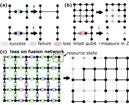
Figure 1: (a) Rotated type-II fusion Gimeno-Segovia et al. (2015); Löbl et al. (2023a) between two nodes of a graph state. If the fusion succeeds (s), the neighbor of one fusion photon gets connected to the neighbor of the other one and vice versa. If the fusion fails (f), there is no connection (b). Photon loss is compensated by removing the neighborhood of the lost qubit from the graph by Z-measurements. If a fusion qubit is lost (lower part of the figure), the neighborhood of both qubits involved in the fusion is measured in the $Z$-basis. (c) The effect of photon loss on a fusion network of star-shaped photonic resource states.

II Background on graph states

Every graph $G=(V,E)$ represents a corresponding quantum state where the vertices of the graph, $V$, are the qubits and the edges, $E$, are entangling operations between the qubits. The graph state can be defined as $\ket{G}=\prod_{(i,j)\in E}C_{ij}\ket{+}^{\otimes{|V|}}$, where $C_{ij}$ is a control phase gate between qubits $i$ and $j$ and $\ket{+}^{\otimes{|V|}}$ is the tensor product where all qubits are in an equal superposition of the two basis states $\ket{0}$ and $\ket{1}$: $\ket{+}=\frac{1}{\sqrt{2}}(\ket{0}+\ket{1})$ Hein et al. (2006).

Measurements can be used to manipulate graph states Hein et al. (2006) and use them for universal quantum computing Raussendorf and Briegel (2001). For this manuscript, it is only necessary to know the effect of two types of measurements: measurement in the $Z$-basis and rotated type-II fusion (a two-photon Bell measurement). For the used resource states, rotated type-II fusion connects the neighborhood of the measured qubits upon success and leaves them mutually unconnected upon failure Gimeno-Segovia et al. (2015); Gimeno-Segovia (2016); Löbl et al. (2023a) (see Fig. 1(a)). The fusion can be implemented using linear optics elements and photon detectors, with the measured photon pattern on the detectors heralding the successful implementation of the fusion Browne and Rudolph (2005); Gimeno-Segovia (2016).

A $Z$-basis measurement of a qubit resulting in $+1$ projects the qubit into the state $\ket{0}$ and corresponds to removing the qubit and its edges from the graph. Measuring $-1$ projects the qubit into $\ket{1}$ and, in addition to the removal of the photon from the graph, applies Pauli $Z$ gates ($Z=\big{(}\begin{smallmatrix}1&0\\ 0&-1\end{smallmatrix}\big{)}$) to the qubits in the neighborhood $N(i)$ of qubit $i$ Hein et al. (2006).

Loss of a qubit can be interpreted as measuring the qubit without knowing the outcome of the measurement, i.e. without knowing whether the gates $\prod_{j\in N(i)}Z_{j}$ have been applied or not. The resulting quantum state is thus a mixed state. To retain a pure quantum state, the qubits in $N(i)$ can be removed from the graph by measuring them in the $Z$-basis Gimeno-Segovia et al. (2015) which is the method that we consider here (see Fig. 1(b)) .

With the method used in this work, a giant cluster state is created above the percolation threshold for photon loss. The obtained cluster state can then be renormalized into a fault-tolerant lattice and be used, e.g., for quantum computing Morley-Short et al. (2017); Herr et al. (2018). For the renormalization, measurements in the $Y$-basis are required as well, as described in Ref. Hein et al. (2006).

Graph states are part of both the larger classes of stabilizer states  Aaronson and Gottesman (2004) and the class of hyper-graph states Rossi et al. (2013). For more detailed information on graph states, we refer the reader to Ref. Hein et al. (2006). An explanation of the required rotated type-II fusion can be found in Fig. 4 of Ref. Gimeno-Segovia et al. (2015) or Fig. A5(d) of Ref. Löbl et al. (2023a). Proposals for generating small resource graph states can be found in Refs. Lindner and Rudolph (2009); Buterakos et al. (2017); Tiurev et al. (2021) and recent experimental realizations in Refs. Schwartz et al. (2016); Coste et al. (2022); Cogan et al. (2023); Thomas et al. (2022); Cao et al. (2023); Maring et al. (2023); Meng et al. (2023).

III Union-find algorithm for simulating photon loss

Generating large-scale entanglement with high tolerance to photon loss is key for implementing quantum computing and networking architectures with photons. We consider the simulation of photon-loss thresholds when the loss is either applied to an existing cluster state or to a fusion network that aims at constructing the cluster state by fusing small resource states. In both cases, it is not obvious which lattice is the best choice Löbl et al. (2023a). In classical bond-site-percolation, a larger vertex degree (coordination number) of the lattice is typically helpful to lower the percolation threshold. In contrast, when a loss is compensated by removing all neighbors of a lost photon by Z-measurements (see Fig. 1(b)), a graph or fusion network with a high vertex degree is particularly sensitive to photon loss. However, a too-low vertex degree makes the graph state or fusion network also fragile due to the higher bond-percolation threshold Kieling et al. (2007); Pant et al. (2019). To find the optimum in between and simulate various fusion lattices, a fast algorithm for computing percolation thresholds for photon loss is required. This algorithm should ideally scale linearly with the number of qubits/photons.

The easiest way to perform classical bond-site-percolation simulations is in the canonical ensemble where the bond (site) probabilities $p_{\text{bond}}$ ($p_{\text{site}}$) are fixed. According to these probabilities, bonds/sites are occupied randomly. Connected components, their size, or whether they percolate the lattice can then be obtained with a time complexity that is linear in the system size by depth- or breadth-first graph traversal Cormen et al. (2022). Constructing a lattice with constant vertex degree (coordination number $z$), $|V|$ nodes, and $|E|=\frac{z}{2}\cdot|V|$ edges takes $\mathcal{O}\left(|V|\right)$ and traversing the graph with e.g. breadth first search takes $\mathcal{O}\left(|V|\right)$ as well Newman and Ziff (2001). This scaling can be slightly improved for two-dimensional percolation by parsing only the boundary of a spanning cluster Ziff et al. (1984); Newman and Ziff (2001). However, this trick does not solve the general issue described in the following.

To make a percolation simulation for $N$ different probabilities of bond occupation ($p_{\text{bond}}$) or site occupation ($p_{\text{site}}$), the computation has to be repeated $N$ times and the running time becomes $\mathcal{O}\left(N\cdot|V|\right)$ Newman and Ziff (2001). When many different probabilities $p_{\text{bond}}$ or $p_{\text{site}}$ are considered, the factor $N$ becomes a major hurdle. For classical bond- and site-percolation simulations, an algorithm that avoids this issue by considering the problem in the microcanonical ensemble Newman and Ziff (2001) has been developed : in such a simulation, the number of occupied bonds/sites is fixed (not the bond/site probability as before). In the corresponding site-percolation simulations, all nodes are initially removed and added to the graph in random order one by one. Bond percolation can be performed analogously by adding bonds as illustrated in Fig. 2(a). Connected graph components of existing nodes are stored and when a new node is added, the corresponding data structure storing the connected components is updated. At the same time, one keeps track of the size of the largest connected component $S(i)$ and a list of booleans $B(i)$ that specifies if percolation (cluster spanning Newman and Ziff (2001)) has been achieved after adding node number $i$. Having computed $\langle S(i)\rangle$ by averaging several simulations of $S(i)$, the expectation value of the largest component size can be computed as a function of $p_{\text{site}}$: 

$$\langle S(p_{\text{site}})\rangle=\sum_{i=0}^{|V|}\langle S(i)\rangle\cdot\binom{|V|}{i}\cdot p_{\text{site}}^{i}\cdot(1-p_{\text{site}})^{|V|-i}$$ (1)

where we compute the binomial coefficients in a normalized way using the iterative method from Ref. Newman and Ziff (2001) (for large $|V|$ a Gaussian approximation of the binomial distribution Malarz (2022) is an alternative). Replacing $S(i)$ by $B(i)$ in the above equation computes the probability of percolation for a given probability $p_{\text{site}}$. It has been shown that the above percolation simulation has a time-complexity of only $\mathcal{O}\left(|V|\right)$ (with no factor $N$) if a suitable union-find algorithm (see below) is used Tarjan (1975); Newman and Ziff (2001).

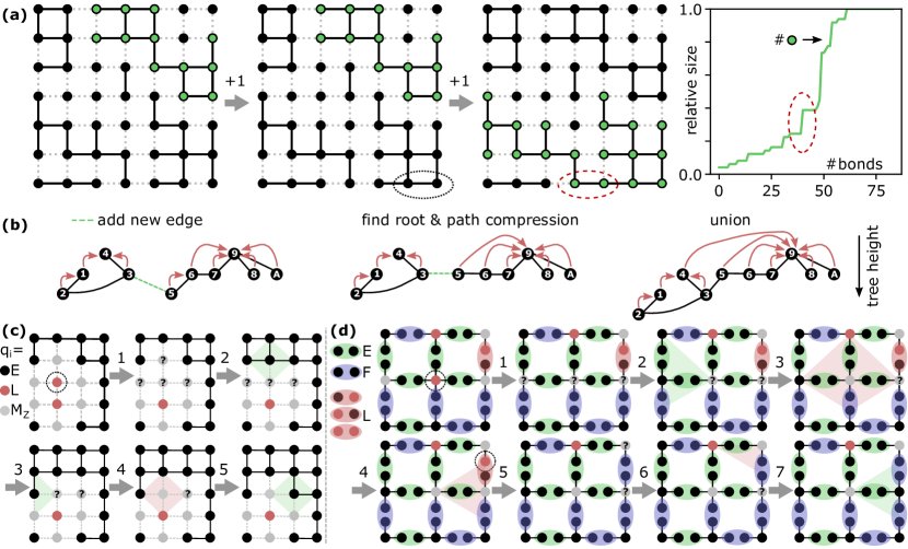
Figure 2: Algorithms to speed-up percolation simulations. (a) The key idea of the Newman-Ziff algorithm Newman and Ziff (2001) illustrated for bond-percolation. Bonds are added one by one and the largest connected component of the graph (green nodes) is monitored. (b) Update the connected graph components in classical bond-percolation Newman and Ziff (2001). In the first step (find), the root nodes of the two components that the new edge connects are identified by following the tree data structure (red arrows). In the second step (union), the two components are merged by connecting the root node of the smaller component to the root node of the larger one. (c) Illustration of algorithm 1 for simulating the effect of loss on a graph state. Initially, two qubits are lost (red nodes) and their neighborhood is therefore measured in the Z-basis (gray). When adding one missing qubit in step 1, several qubits in the neighborhood need to be potentially updated. This update is done in steps $2-5$ where the neighborhoods of all potentially affected nodes are checked for lost qubits. When none of a qubit’s neighbors are lost, there is no need anymore to measure it in the Z-basis and it is added to the graph. (d) Illustration of algorithm 2 for simulating the effect of loss when creating a large graph state by fusing star-shaped resource states. In step 1, a lost central qubit is added. All qubits that are not lost and connected to the added qubit by a successful fusion potentially need to be updated. The update is done in steps $2-4$ by applying the rules from Fig. 1 to all potentially affected qubits. In step 5, a previously lost fusion qubit is added. The subsequent update algorithm (steps 6, 7) is the same as before with the difference that only the central node belonging to the added fusion qubit and the central node belonging to its fusion partner need to be updated.

Critical to implementing such an algorithm is a data structure that is efficiently keeping track of the graph and its connected components as well as a method to update it when adding an edge/node. As in Ref. Newman and Ziff (2001) we use a tree data structure Galler and Fisher (1964) where every node is either a root node representing an isolated graph component or it points to a parent node that is part of the same graph component. An example of such a data structure and how to update it for bond-percolation is shown in Fig. 2(b) where the simulated graph is drawn in black and the tree data structure is illustrated by the red arrows. Adding a previously missing edge is done by an update of the graph and the tree data structure using the union-find algorithm from Ref. Newman and Ziff (2001): following the tree data structure, the algorithm first determines the root nodes of the two graph components that the new edge connects (find). (To reduce the length of subsequently traversed paths, we employ path compression Tarjan (1975); Newman and Ziff (2001) such that the parent node for all nodes along the path is updated to the root node.) If the two root nodes are different, the graph components are merged by making one of the root nodes point to the other (union). To improve the performance, one attaches the smaller component to the larger one (weighted union Tarjan (1975); Newman and Ziff (2001)). This union operation is done in $\mathcal{O}\left(1\right)$ steps as opposed to an approach based on a look-up table storing the graph component for every node in an array. The latter would need $\mathcal{O}\left(1\right)$ for a single find operation but $\mathcal{O}\left(|V|\right)$ to determine all nodes of the cluster that must be updated in a union. The overall time complexity would become $\mathcal{O}\left(|V|^{2}\right)$. In contrast, the combination of path compression and weighted union using the tree data structure results in a practically linear time scaling, respectively $\mathcal{O}\left(|V|\right)$  . This result is important for efficiently performing classical bond-site percolation simulations Newman and Ziff (2001) and also for efficient union-find decoders in quantum error correction Delfosse and Nickerson (2021).

Adding a previously missing node in a site percolation simulation is done similarly Newman and Ziff (2001): the algorithm first adds the new node as an isolated single-node graph component. Then it adds the edge to the first neighbor and updates the graph like in the case of bond percolation . This procedure is repeated for all the other neighbors and we denote the algorithm from Ref. Newman and Ziff (2001) for adding a previously missing node algorithm 0.

In the following, we describe algorithms that use the tools described so far to efficiently simulate photon loss as a percolation problem. Algorithm 1 applies to the loss tolerance of a given cluster state, and Algorithm 2 computes the loss tolerance of fusion networks of all-photon star-shaped resource states. Note that to apply Algorithms 1 and 2 in practice, one needs to know where photon loss has happened Morley-Short et al. (2017) (heralded loss). When loss is unheralded, challenging quantum non-demolition detection of the loss Stricker et al. (2020) would be required to find connected paths in the lattice. To circumvent this issue, we consider another model where the central qubits of the star-shaped resource states are spins, and hence one can typically assume that they cannot be lost. All the photons are measured in type-II fusions Browne and Rudolph (2005), where photon loss is heralded Gimeno-Segovia et al. (2015); Gimeno-Segovia (2016). The corresponding model can be efficiently simulated with Algorithm 3. Finally, Algorithm 4 simulates a corresponding adaptive scheme where fusions can be repeated until success by generating new fusion photons on-demand. In the case of Algorithms 3, 4, the computed percolation thresholds present necessary and sufficient conditions for measurement-based quantum computing Löbl et al. (2023a) after lattice renormalization Herr et al. (2018). In the case of Algorithms 1 and 2 (all-photonic case), the computed thresholds are only meaningful under the assumption that loss of non-fusion photons is heralded Morley-Short et al. (2017).

III.1 Update rule for graph states and fusion networks

Similar to the Newman-Ziff algorithm Newman and Ziff (2001) we assume initially that all photons are lost and then add them one by one keeping track of the largest connected graph component or checking if a graph component percolates. However, new rules are required to update the graph when a previously lost photon is added.

First, we consider an existing photon cluster state suffering loss. The update of the cluster state after adding a previously lost qubit $i$ is complicated by the fact that the neighborhood $N(i)$ of a lost qubit is measured in the Z-basis Gimeno-Segovia et al. (2015). When adding a missing qubit, those neighbors potentially have to be updated and added to the graph if there is no longer any need to measure them in the Z-basis. We assign a label $q_{i}$ to every central qubit of a resource state: $q_{i}=L$ meaning that the qubit is lost, $q_{i}=M_{Z}$ meaning that the qubit needs to be measured in the Z-basis, or $q_{i}=E$ meaning that the qubit exists (not lost nor has to be measured in Z, and therefore is part of the graph/cluster state). Algorithm 1 describes the corresponding data structure update when changing the label of a qubit in a cluster state (no fusion network) from lost to not lost (decreasing the number of lost photons by one). The algorithm is illustrated in Fig. 2(c).

(1) $q_{i}:=M_{Z}$;

(2) $\tilde{V}:=\{j\in N(i)\mid q_{j}=M_{Z}\}\cup\{i\}$;

(3) for $j\in\ \tilde{V}$ do

                 if $\left(\nexists\ k\in N(j):q_{k}=L\right)$ then

                            $q_{j}:=E$;

                            add node $j$ via algorithm 0;

          

          

Algorithm 1 add lost qubit ($q_{i}=L$) to the graph

In the first step, the label of the lost qubit $i$ is changed to $q_{i}=M_{Z}$ indicating that it is not lost anymore. In the second step, a list $\tilde{V}$ of all potentially affected qubits is created (all qubits in the neighborhood $N(i)$ of qubit $i$ as well as qubit $i$ itself). In the final step, the neighborhood of all qubits in $\tilde{V}$ is checked for lost qubits. If a lost qubit is still found in the neighborhood of a qubit in $\tilde{V}$, no update needs to be done. If no lost qubit in the neighborhood is found, the corresponding qubit label is updated to $E$. In the latter case, the corresponding qubit was only affected by the loss of qubit $i$ and can be added to the graph once qubit $i$ is not lost anymore. Adding qubits to the graph is done with algorithm 0 from Ref. Newman and Ziff (2001).

The above algorithm is useful for estimating the loss tolerance of a pre-existing cluster state. A more realistic experimental situation is a scenario where a large graph state is constructed by fusing many small star-shaped resource states (Fig. 1(c)) Gimeno-Segovia et al. (2015); Löbl et al. (2023a). As described above, we consider rotated type-II fusion with two fusion photons per edge (success probability $p_{s}=0.5$ Gimeno-Segovia (2016); Löbl et al. (2023a)) . Every photon (either in the center of a star-shaped resource state or a fusion photon on the leaf of it) can be lost with a uniform probability $p_{loss}=1-\eta$. We assign different labels to every edge $e_{ij}$ ($i$, $j$ are the numbers of the central qubits of the star-shaped resource states that the edge connects upon successful fusion): $e_{ij}=L$ when at least one of the photons on this edge is lost (probability $1-\eta^{2}$), $e_{ij}=E$ when the corresponding fusion was successful (probability $p_{s}\eta^{2}$), and $e_{ij}=F$ when the fusion failed but no photon was lost (probability $(1-p_{s})\eta^{2}$).

When adding a previously lost photon, there are two cases: the photon can be a central qubit of the star-shaped resource state or it can be a fusion qubit.

We first consider the case of adding a lost central qubit to the corresponding fusion network. The graph update is done by Algorithm 2 (see Fig. 2(d) for an illustration).

(1) $q_{i}:=M_{Z}$;

(2) $\tilde{V}:=\{j\in N(i)\mid q_{j}=M_{Z}\land\ e_{ij}=E\}\cup\{i\}$;

(3) for $j\in\tilde{V}$ do

                 if $\left(\nexists\ k\in N(j):q_{k}=L\land\ e_{jk}=E\right)\land$

                 $\left(\nexists\ k\in N(j):e_{jk}=L\right)$ then

                            $q_{j}:=E$;

                            add node $j$ via algorithm 0;

          

          

Algorithm 2 add lost central qubit ($q_{i}=L$) to the fusion network

Here $N(i)$ refers to all qubits in the center of other star-shaped resource states that one tries to connect to qubit $i$ by a fusion. In the first step, the label of the lost qubit is changed to $q_{i}:=M_{Z}$ as in Algorithm 1. In the second step, a list $\tilde{V}$ of all potentially affected qubits is created. A qubit $j\neq i$ can only be affected by a change of qubit $i$ when there is a connection between both qubits obtained by a successful fusion ($e_{ij}=E$). In the final step, all potentially affected qubits $j\in\tilde{V}$ are updated. A qubit can only be added ($q_{j}:=E$) when it is not connected to a lost qubit by a successful fusion ($\nexists\ k\in\ N(j):q_{k}=L\land\ e_{jk}=E$) and no fusion photon on any of its edges is lost ($\nexists\ k\in\ N(j):e_{jk}=L$).

Next, we consider the case where the lost qubit is a fusion qubit between two central qubits $i$, $j$. Here, Algorithm 2 is slightly modified: first, the edge $e_{ij}$ must be updated iff the fusion partner of the new qubit is not lost (otherwise $e_{ij}$ keeps the label $L$). In this case, the edge label is updated to $e_{ij}=F$ or $e_{ij}=E$ with probabilities of $1-p_{s}=p_{s}=1/2$ and only then steps 2 and 3 need to be done. Second, the list of affected central qubits in step 2 must be changed to $\tilde{V}=\{i,j\}$. Algorithm 3 describes the corresponding graph update rule.

(1) if both qubits on $e_{ij}$ are not lost then

                  with probability $p_{s}$: $e_{ij}:=E$

                  otherwise: $e_{ij}:=F$;

     

            else

                       skip steps 2, 3;

          

           (2) $\tilde{V}:=\{k\in\{i,j\}\mid q_{k}\neq L\}$;

           (3) for $l\in\tilde{V}$ do

                           if $\left(\nexists\ k\in N(l):q_{k}=L\land\ e_{lk}=E\right)\land$

                            $\left(\nexists\ k\in N(l):e_{lk}=L\right)$ then

                                      $q_{l}:=E$;

                                      add node $l$ via algorithm 0;

                    

                    

Algorithm 3 add lost fusion qubit on edge $e_{ij}$

III.2 Running time analysis

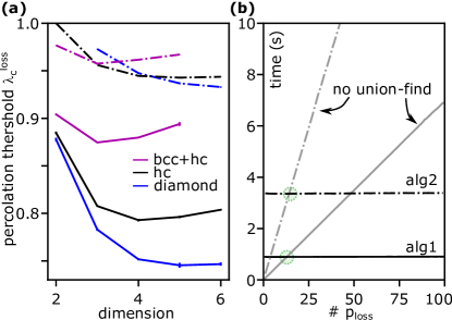
Figure 3: (a) Percolation threshold for photon loss $\lambda_{c}^{loss}$ for the diamond, hypercubic (hc), and bcc+hc lattices. $\lambda_{c}^{loss}$ has two different meanings here: the solid lines show simulations of given cluster states suffering photon loss, and the dashed lines are corresponding simulations of a fusion network with star-shaped resource states. (b) Running time for simulating a 3D simple-cubic lattice with $10^{6}$ nodes (not the simulations in part (a)) . Without algorithm 1, the simulation time increases linearly when the number of values for $p_{loss}$ increases. When using Algorithm 1, the simulation time is constant, independent of how many different values for $p_{loss}$ are simulated.

Fig. 3(a) shows simulations of the loss tolerance of cluster states with algorithm 1. It also shows simulations of corresponding fusion networks using star-shaped resource states (simulated using algorithms 2, 3). As expected, the running time of these simulations is independent of the number of simulated photon loss probabilities (see Fig. 3(b)). Without these algorithms, a new graph traversal is performed for every photon loss probability leading to a time that is linear in the number of simulated loss probabilities. Fig. 3(b) shows that the union-find algorithms become more efficient when about a dozen different values for $p_{loss}$ are simulated. The speed advantage is key for simulating the loss tolerance of large fusion networks Löbl et al. (2023a).

The above algorithms allow performing percolation simulations of various lattices representing cluster states or fusion networks and the running time is independent of how many values of $p_{loss}$ are simulated. We expect that the running time as a function of the system size (number of vertices in the cluster state or fusion network) scales identically to Ref. Newman and Ziff (2001) (and so practically linear in system size). The reason is that the overhead of Algorithms 1 and 2 compared to Algorithm 0 is a constant prefactor.

III.3 Update rule for an adaptive scheme

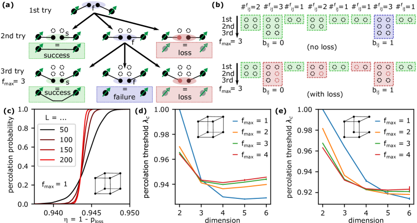
Figure 4: (a) Adaptive scheme where fusions are repeated until either success, heralded photon loss, or until $f_{max}$ trials are reached. This scheme can be realized using quantum emitters with a spin (drawn as black dots with green arrows) where adjacent quantum emitters generate new fusion photons if an attempt to entangle them with a fusion fails (see e.g. Ref. Tiurev et al. (2021) for a system providing the required spin-photon entanglement). When there is a loss, both quantum emitter spins need to be reinitialized (measured in the $Z$-basis) as indicated in gray. (b) Schematic illustration of the data structure used for keeping track of the fusion results when sweeping the number of lost photons. In the absence of loss (upper part), the overall fusion succeeds except when all individual fusion attempts fail ($b_{ij}=1$). As long as there is one loss in the fusion ($c_{ij}<2\cdot\#^{f}_{ij}$), it terminates by re-initializing the spin qubit. (c) Simulation of the simple cubic fusion lattice with $f_{max}=1$. (d) Percolation threshold of the hypercubic fusion lattice for different values of $f_{max}$. (e) Corresponding simulation of the generalized diamond lattice.

So far, we have explored how the Newman-Ziff algorithm can be applied to simulate the effect of photon loss in fusion networks where all fusions are performed at once (ballistically). In such a scheme, every fusion is performed no matter what the outcome of the other fusions is. In adaptive schemes, a fusion attempt may depend on the previous measurement record and that makes it more challenging to apply algorithms as the ones described so far. In the previous algorithms, we initially labeled all photons as lost ($L$) and added them one by one. The question is then how the algorithm should work if the graph structure or the overall number of photons is flexible and it is therefore unclear how many photons exist and where in the graph they are used. Below, we give an example showing that Newman-Ziff-type algorithms can nevertheless be applied to some adaptive schemes.

We consider a scheme where the central nodes of the star-shaped resource states are spins in quantum emitters. To establish a connection between two emitters, each of them creates a photon entangled with it, e.g. by using a suitable optical pulse Lindner and Rudolph (2009); Tiurev et al. (2021). When the fusion succeeds, we proceed with no further actions. When the fusion fails, both quantum emitters generate a new photon entangled with them, and the fusion is repeated as illustrated in Fig. 4(a). This procedure is repeated until the fusion either succeeds, fails after a maximum number of repetitions $f_{max}$, or heralds photon loss before. In the latter case, the two quantum emitter spin qubits are removed from the graph by Z-measurements as before . In this model, the probabilities that the fusion attempts on a certain edge succeed ($p_{S}$), fail ($p_{F}$), or terminate with a loss ($p_{L}$) are Lim et al. (2006); de Gliniasty et al. (2023):

$$p_{F}=\left(\eta^{2}(1-p_{s})\right)^{f_{max}}=\alpha^{f_{max}}$$ (2)

$$p_{S}=\eta^{2}\cdot p_{s}\cdot\sum_{k=0}^{f_{max}-1}(\eta^{2}(1-p_{s}))^{k}=\frac{\eta^{2}}{2}\cdot\frac{\alpha^{f_{max}}-1}{\alpha-1}$$ (3)

$$p_{L}=1-p_{F}-p_{S}$$ (4)

where we have used $p_{s}=0.5$ for a single fusion attempt and defined $\alpha\equiv\eta^{2}/2$.

The described adaptive approach is related to well-known schemes for creating spin-spin entanglement via Bell-measurements and corresponding repeat-until success schemes Barrett and Kok (2005); Lim et al. (2005, 2006). The difference is that it is still in some sense ballistic because the maximum number of repetitions is bounded. This avoids unbounded delays from arbitrary many repetitions of a single fusion attempt. Furthermore, fusion repetitions can be performed in parallel as the outcome of a fusion does not influence what is done at different nodes elsewhere (the scheme is only locally adaptive).

Note that this slightly adaptive approach has a lower loss tolerance compared to repeat-until success schemes that employ multiple qubits per node Choi et al. (2019). In turn, the scheme can be applied for emitters with only a single spin per node. Higher thresholds to photon loss can principally be achieved with an adaptive divide and conquer approach Barrett and Kok (2005); Duan and Raussendorf (2005); Lim et al. (2006) or loss-tolerant encoding Varnava et al. (2008); Borregaard et al. (2020); Bell et al. (2023). However, both methods introduce a substantial overhead for creating a large entangled graph state.

Our algorithm to simulate the loss tolerance of the adaptive scheme described above consists of two main steps. In the first step, we assume that there is no photon loss and determine for every edge $e_{ij}$ how many fusion attempts are required for the fusion to succeed. We label this number of fusion attempts $\#^{f}_{ij}$ and it is determined by tossing a random coin until the coin indicates a success. The frequency distribution of the number $\#^{f}_{ij}$ is thus exponentially smaller for higher values of $\#^{f}_{ij}$. When none of the $f_{max}$ fusions succeed, we keep track of that by a Boolean array $b_{ij}$ where $b_{ij}=0$ indicates fusion success and $b_{ij}=1$ fusion failure. The number $\#^{f}_{ij}$ determines how many potentially lost photons we have to consider for the edge $e_{ij}$, namely exactly $2\cdot\#^{f}_{ij}$ as illustrated in Fig. 4(b). The reason is that after $\#^{f}_{ij}$ fusion attempts, no further fusions on $e_{ij}$ are performed because the fusion either succeeded, failed when $\#^{f}_{ij}=f_{max}\land b_{ij}=1$, or because there has been a heralded photon loss before. So without loss, the overall number of fusion photons is $\sum_{ij}2\cdot\#^{f}_{ij}$.

In the second step, the fusion photons of all the edges are labeled as lost. As before, they are added one by one in random order while keeping track of the connected graph components. In that process, an edge keeps the label $e_{ij}=L$ until all its $2\cdot\#^{f}_{ij}$ fusion qubits are not lost anymore. We count on every edge $e_{ij}$ the number of photons that are not lost with a counter variable $c_{ij}$ (initially zero and increases whenever a fusion photon is added on edge $e_{ij}$). A change on the graph needs to be done once $c_{ij}$ reaches $2\cdot\#^{f}_{ij}$ (before the attempt to establish a connection between nodes $i$ and $j$ always terminates with a photon loss). Algorithm 4 describes how this update is done. As the central qubits $q_{i}$ are quantum emitters (and thus cannot be lost), Algorithm 4 differs from Algorithm 3 in steps 2, 3).

The described method to simulate the adaptive scheme is justified because it fulfills the following condition: assume a fraction $\tilde{\eta}$ of all fusion photons has been labeled as not lost. Then the probabilities that the result of the fusion attempts on a random edge $e_{ij}$ is failure, success, or loss are equal to the probabilities $p_{F},p_{S},p_{F}$ in Eq. 2, 3, 4. Thus Eq. 1 (with $|V|$ being replaced by the number of all photons $\sum_{ij}2\cdot\#^{f}_{ij}$ and the averaging being done outside the sum) can be used to get the expectation value of the largest graph component size as a function of $p_{loss}=1-\tilde{\eta}$.

(1) $c_{ij}:=c_{ij}+1$;

     if $c_{ij}=2\cdot\#^{f}_{ij}$ then

                 if $b_{ij}=1$ then

                            $e_{ij}=F$;

          

                      else

                                 $e_{ij}=E$;

               

               

                     else

                                skip all following steps;

                    

                     (2) $\tilde{V}:=\{i,j\}$;

                     (3) for $l\in\tilde{V}$ do

                                     if $\left(\nexists\ k\in N(l):e_{kl}=L\right)$ then

                                                $q_{l}:=E$;

                                                add node $l$ via algorithm 0;

                              

                              

Algorithm 4 add previously lost fusion photon on edge $e_{ij}$.

An alternative method for boosting the fusion success probability uses ancilla entangled photon pairs Grice (2011). The probabilities for fusion success and loss of a fusion photon differ from Eqs. 3, 4 as $2^{n}$ photons are used for every fusion ($n=1$ being the standard fusion) to achieve a success probability of $1-1/2^{n}$. We therefore have: $p_{F}=\eta^{(2^{n})}/2^{n}$, $p_{S}=\eta^{(2^{n})}\cdot(1-1/2^{n})$, $p_{L}=1-p_{F}-p_{S}$. Using $2^{n}$ photons per fusion can be simulated with the approach from before by setting $2\cdot\#^{f}_{ij}=2^{n}$. Once all fusion photons exist, the fusion is set to failure with a probability of $1/2^{n}$ and success otherwise.

For the all-photonic boosting, the number of photons is fixed and it thus would be possible to make a modified Newman-Ziff algorithm by adding lost fusions one by one (instead of virtually adding lost photons). The size of the largest connected graph component is then obtained as a function of the number of fusions with no lost photons. Using the relation between $\eta$ and $p_{L}$ one can convert such a simulation into the largest connected graph component as a function of $\eta$ rescaling the $x$-axis. For the discussed adaptive scheme, such a simplification is, however, not possible as $p_{S}/p_{F}$ is not constant as a function of $\eta$. Even if one would compute $p_{S}/p_{F}$ (by converting $p_{L}$ into $\eta$) in every step where a previously lossy fusion is added, all the fusions that were added before would appear in a ratio $p_{S}/p_{F}$ that is inconsistent with the current fraction of not lossy fusions (resp. $p_{L}$). Also when fusion photons as well as other photons are lost (Algorithm 2), we believe that the only feasible approach is virtually adding photons one by one and doing the required data structure update in every step.

III.4 Adaptive Simulations

Fig. 4(c) shows a percolation simulation of the simple cubic lattice for different lattice sizes. In this simulation, only one fusion attempt per edge is made which corresponds to the ballistic scheme and therefore can be simulated by either Algorithm 3 or Algorithm 4. Figs. 4(d,e) show the obtained percolation thresholds for the loss tolerance of the hypercubic (hc) and the generalized diamond fusion lattice Van der Marck (1998) in several dimensions. Using Algorithm 4, these simulations are done for different values of the maximum number of fusion repetitions ($f_{max}$). We observe that the adaptive scheme investigated here improves the loss tolerance for the low-dimensional lattices but makes it worse in higher dimensions. This trend is observed for all fusion lattices that we investigate. The reason for the worse loss tolerance is that repeating the fusions until success increases the chance that the fusion terminates by photon loss. Using all-photonic boosting Grice (2011); Ewert and van Loock (2014) would have a similar issue. Of course, the illustrated adaptive scheme is not ideal: fusions are for instance performed even if it is known that one of the involved quantum-emitter qubits must be measured in $Z$ due to a loss in a previous fusion. Problems like this can be avoided with more sophisticated adaptive schemes.

IV Summary and Outlook

We have shown that it is possible to use a modification of Newman and Ziff’s algorithm Newman and Ziff (2001) for non-standard percolation models motivated by photon loss in cluster states and fusion networks. We have considered ballistic fusion networks where many resource states are connected by simultaneous probabilistic fusions and an adaptive scheme where fusions are repeated until success. Speeding up the simulation of such architectures allows running optimizations over many fusion lattices Löbl et al. (2023a). Mitigating the photon loss with such optimizations is relevant as loss is arguably the biggest challenge for photonic quantum computing and networking.

We have considered star-shaped resource states but our algorithms also apply when resource states such as branched chains are used (like star-shaped resource states these states can be generated by a single quantum emitter Paesani and Brown (2023)). The only condition for our algorithms to work is that all fusion photons are leaf nodes of the resource state graphs and thus only have a single neighbor (which can also apply to some types of higher-dimensional states that cannot be generated by a single quantum emitter Economou et al. (2010); Li et al. (2022)). Whether similar algorithms also can be used when fusing other types of states such as linear chain graph states Lindner and Rudolph (2009); Thomas et al. (2022) could be investigated in future works. Another interesting direction is investigating if similar algorithms can be developed for efficiently simulating adaptive schemes where a policy, more sophisticated than repeat until success, is applied to decide if a fusion is performed or not.

Finally, we hope that our results might be inspiring or useful for other applications in quantum information: percolation models can be applied to quantum networks Acín et al. (2007), the bond-percolation threshold of the syndrome graph determines the loss threshold of various topological quantum error-correction codes Stace et al. (2009); Barrett and Stace (2010); Auger et al. (2018); Stricker et al. (2020); Bartolucci et al. (2023), and qubit loss in color codes can be simulated with modified percolation models Vodola et al. (2018); Amaro et al. (2020). In addition, logical errors in topological codes are operators that span around the code Dennis et al. (2002). The transition where errors plus the decoder output give a percolating operator is thus a lower bound for the error threshold Hastings et al. (2014). All these points indicate that similar algorithms as the ones developed here could improve the analysis of quantum error correction in general.

V Acknowledgment

We would like to thank Love A. Pettersson for fruitful discussions and Daniel Löbl for support with the C-implementation. We are grateful for financial support from Danmarks Grundforskningsfond (DNRF 139, Hy-Q Center for Hybrid Quantum Networks). S.P. acknowledges funding from the Marie Skłodowska-Curie Fellowship project QSun (nr. 101063763), from the VILLUM FONDEN research grant VIL50326, and support from the NNF Quantum Computing Programme.

VI Appendix: source code

VI.1 General description

Our simulation program is written in the programming language C and can be freely downloaded Löbl et al. (2023b). It can be used to simulate the loss tolerance of fusion networks with various lattice geometries in several dimensions. Furthermore, it enables simulating the loss tolerance of an existing cluster state as well as classical bond-site and site-bond percolation simulations. The following explanation focuses on simulating non-adaptive fusion networks but all the other simulations can be performed very similarly with the provided source code.

Every simulation consists of three main steps: In the first step, a certain lattice with fixed size and dimension is built. We use an adjacency list to represent the graphs/fusion lattices keeping the data structure analogous to Ref. Newman and Ziff (2001). Therefore, other lattices can be easily built or taken from the literature where a similar implementation is used Malarz (2022). In the second step, the effect of the random process of photon loss and fusion failure is simulated. Since the fusion probability is a fixed parameter given by the physical implementation, we first randomly set fusions to success/fail. The effect of photon loss is then simulated using the described algorithms where all photons are labeled as lost initially and then added one by one. During that process, we keep track of the largest component size $S(i)$ or a Boolean array $B(i)$ specifying if percolation (cluster spanning) has been achieved. This second part of the simulation is repeated several times to get good statistics by averaging. In the third step, Eq. 1 is used to compute the probability of percolation or the expectation value of the largest component size as a function of the loss.

For the graph construction in the first step, we provide several functions with which lattices such as hypercubic, diamond, bcc, and fcc can be built in a dimension of choice. In particular, our implementation allows simulating all lattices from Ref. Kurzawski and Malarz (2012) including their higher-dimensional generalizations, all lattices from Ref. Van der Marck (1998) except the Kagome lattice, and hypercubic lattices with extended neighborhoods Malarz and Galam (2005); Xun and Ziff (2020); Zhao et al. (2022).

VI.2 Verification of the implementation

To verify our lattice constructions, we have performed classical site-percolation simulations of lattices with known percolation thresholds Van der Marck (1998); Kurzawski and Malarz (2012). These simulations can be found in Ref. Löbl et al. (2023a) where we have simulated two- to six-dimensional lattices that, for periodic boundaries, correspond to various $k$-regular graphs with $k\in[3..50]$. Additionally, we compute here a few bond-percolation thresholds. For instance, for the bond-percolation thresholds of the generalized diamond lattices Van der Marck (1998), we find $\lambda_{bond}=0.6529(10),\,0.3893(7),\,0.2709(18),\,0.2072(15),\,0.1646(43)$ for dimensions $2-6$ respectively which is in agreement with Refs. Sykes and Essam (1964); Xu et al. (2014); Van der Marck (1998). Furthermore, we find $\lambda_{bond}=0.24886\pm 0.00002$ for the bond-percolation threshold of the simple-cubic lattice (roughly agrees with Ref. Wang et al. (2013)) which also represents the syndrome graph of the RHG lattice Raussendorf et al. (2006). For the latter, we find a bond-percolation threshold of $\lambda_{bond}=0.3845(1)$ and a site-percolation threshold of $\lambda_{site}=0.4220(5)$.

Algorithms 1, 2, 3, 4 do not correspond to a percolation model that has been used in the literature. To verify that the implementation of these algorithms is correct, we have implemented several redundant functions for the corresponding percolation models without any Newman-Ziff-type algorithm. (see read-me file of the code repository Löbl et al. (2023b) for more information). We have performed several tests for which the results were consistent between the different implementations.

References

- Hein et al. (2006) M. Hein, W. Dür, J. Eisert, R. Raussendorf, M. Nest, and H.-J. Briegel, arXiv quant-ph/0602096 (2006).
- Raussendorf and Briegel (2001) R. Raussendorf and H. J. Briegel, Phys. Rev. Lett. 86, 5188 (2001).
- Raussendorf et al. (2003) R. Raussendorf, D. E. Browne, and H. J. Briegel, Phys. Rev. A 68, 022312 (2003).
- Gimeno-Segovia et al. (2015) M. Gimeno-Segovia, P. Shadbolt, D. E. Browne, and T. Rudolph, Phys. Rev. Lett. 115, 020502 (2015).
- Paesani and Brown (2023) S. Paesani and B. J. Brown, Phys. Rev. Lett. 131, 120603 (2023).
- Morley-Short et al. (2017) S. Morley-Short, S. Bartolucci, M. Gimeno-Segovia, P. Shadbolt, H. Cable, and T. Rudolph, Quantum Sci. Technol. 3, 015005 (2017).
- Herr et al. (2018) D. Herr, A. Paler, S. J. Devitt, and F. Nori, npj Quantum Information 4, 27 (2018).
- Kieling et al. (2007) K. Kieling, T. Rudolph, and J. Eisert, Phys. Rev. Lett. 99, 130501 (2007).
- Pant et al. (2019) M. Pant, D. Towsley, D. Englund, and S. Guha, Nat. Commun. 10, 1070 (2019).
- Browne and Rudolph (2005) D. E. Browne and T. Rudolph, Phys. Rev. Lett. 95, 010501 (2005).
- Knill et al. (2001) E. Knill, R. Laflamme, and G. J. Milburn, Nature 409, 46 (2001).
- Hacker et al. (2016) B. Hacker, S. Welte, G. Rempe, and S. Ritter, Nature 536, 193 (2016).
- Löbl et al. (2023a) M. C. Löbl, S. Paesani, and A. S. Sørensen, arxiv:2304.03796 (2023a).
- Chanana et al. (2022) A. Chanana, H. Larocque, R. Moreira, J. Carolan, B. Guha, E. G. Melo, V. Anant, J. Song, D. Englund, D. J. Blumenthal, et al., Nat. Commun. 13, 7693 (2022).
- Uppu et al. (2021) R. Uppu, L. Midolo, X. Zhou, J. Carolan, and P. Lodahl, Nat. Nanotechnol. 16, 1308 (2021).
- Tomm et al. (2021) N. Tomm, A. Javadi, N. O. Antoniadis, D. Najer, M. C. Löbl, A. R. Korsch, R. Schott, S. R. Valentin, A. D. Wieck, A. Ludwig, et al., Nat. Nanotechnol. 16, 399 (2021).
- Ding et al. (2023) X. Ding, Y.-P. Guo, M.-C. Xu, R.-Z. Liu, G.-Y. Zou, J.-Y. Zhao, Z.-X. Ge, Q.-H. Zhang, M.-C. C. Hua-Liang Liu, et al., arxiv:2311.08347 (2023).
- Varnava et al. (2008) M. Varnava, D. E. Browne, and T. Rudolph, Phys. Rev. Lett. 100, 060502 (2008).
- Stauffer and Aharony (2018) D. Stauffer and A. Aharony, Introduction to percolation theory (CRC press, 2018).
- Newman and Ziff (2001) M. E. J. Newman and R. M. Ziff, Phys. Rev. E 64, 016706 (2001).
- Cabello et al. (2011) A. Cabello, L. E. Danielsen, A. J. López-Tarrida, and J. R. Portillo, Phys. Rev. A 83, 042314 (2011).
- Adcock et al. (2020) J. C. Adcock, S. Morley-Short, A. Dahlberg, and J. W. Silverstone, Quantum 4, 305 (2020).
- Gimeno-Segovia (2016) M. Gimeno-Segovia, Towards practical linear optical quantum computing, Ph.D. thesis, Imperial College London (2016).
- Thomas et al. (2022) P. Thomas, L. Ruscio, O. Morin, and G. Rempe, Nature 608, 677 (2022).
- Warburton (2013) R. J. Warburton, Nat. Mater. 12, 483 (2013).
- Lodahl et al. (2015) P. Lodahl, S. Mahmoodian, and S. Stobbe, Rev. Mod. Phys. 87, 347 (2015).
- Atatüre et al. (2018) M. Atatüre, D. Englund, N. Vamivakas, S.-Y. Lee, and J. Wrachtrup, Nat. Rev. Mater. 3, 38 (2018).
- Shandilya et al. (2022) P. K. Shandilya, S. Flågan, N. C. Carvalho, E. Zohari, V. K. Kavatamane, J. E. Losby, and P. E. Barclay, J. Light. Technol. 40, 7538 (2022).
- Montblanch et al. (2023) A. R.-P. Montblanch, M. Barbone, I. Aharonovich, M. Atatüre, and A. C. Ferrari, Nat. Nanotechnol. 18, 555 (2023).
- Simmons (2023) S. Simmons, arXiv:2311.04858 (2023).
- Lindner and Rudolph (2009) N. H. Lindner and T. Rudolph, Phys. Rev. Lett. 103, 113602 (2009).
- Economou et al. (2010) S. E. Economou, N. Lindner, and T. Rudolph, Phys. Rev. Lett. 105, 093601 (2010).
- Grice (2011) W. P. Grice, Phys. Rev. A 84, 042331 (2011).
- Ewert and van Loock (2014) F. Ewert and P. van Loock, Phys. Rev. Lett. 113, 140403 (2014).
- Bayerbach et al. (2023) M. J. Bayerbach, S. E. D’Aurelio, P. van Loock, and S. Barz, Sci. Adv. 9, eadf4080 (2023).
- Löbl et al. (2023b) M. C. Löbl et al., “perqolate,” https://github.com/nbi-hyq/perqolate (2023b).
- Aaronson and Gottesman (2004) S. Aaronson and D. Gottesman, Phys. Rev. A 70, 052328 (2004).
- Looi et al. (2008) S. Y. Looi, L. Yu, V. Gheorghiu, and R. B. Griffiths, Phys. Rev. A 78, 042303 (2008).
- Rossi et al. (2013) M. Rossi, M. Huber, D. Bruß, and C. Macchiavello, New J. Phys. 15, 113022 (2013).
- Buterakos et al. (2017) D. Buterakos, E. Barnes, and S. E. Economou, Phys. Rev. X 7, 041023 (2017).
- Tiurev et al. (2021) K. Tiurev, P. L. Mirambell, M. B. Lauritzen, M. H. Appel, A. Tiranov, P. Lodahl, and A. S. Sørensen, Phys. Rev. A 104, 052604 (2021).
- Schwartz et al. (2016) I. Schwartz, D. Cogan, E. R. Schmidgall, Y. Don, L. Gantz, O. Kenneth, N. H. Lindner, and D. Gershoni, Science 354, 434 (2016).
- Coste et al. (2022) N. Coste, D. Fioretto, N. Belabas, S. Wein, P. Hilaire, R. Frantzeskakis, M. Gundin, B. Goes, N. Somaschi, M. Morassi, et al., arXiv:2207.09881 (2022).
- Cogan et al. (2023) D. Cogan, Z.-E. Su, O. Kenneth, and D. Gershoni, Nat. Photon. 17, 324–329 (2023).
- Cao et al. (2023) H. Cao, L. M. Hansen, F. Giorgino, L. Carosini, P. Zahalka, F. Zilk, J. C. Loredo, and P. Walther, arXiv:2308.05709 (2023).
- Maring et al. (2023) N. Maring, A. Fyrillas, M. Pont, E. Ivanov, P. Stepanov, N. Margaria, W. Hease, A. Pishchagin, T. H. Au, S. Boissier, et al., arXiv:2306.00874 (2023).
- Meng et al. (2023) Y. Meng, M. L. Chan, R. B. Nielsen, M. H. Appel, Z. Liu, Y. Wang, B. Nikolai, A. D. Wieck, A. Ludwig, L. Midolo, A. Tiranov, A. S. Sørensen, and P. Lodahl, arxiv:2310.12038 (2023).
- Cormen et al. (2022) T. H. Cormen, C. E. Leiserson, R. L. Rivest, and C. Stein, Introduction to algorithms (MIT press, 2022).
- Ziff et al. (1984) R. M. Ziff, P. T. Cummings, and G. Stells, J. Phys. A: Math. Gen. 17, 3009 (1984).
- Choi and Yu (2019) J.-O. Choi and U. Yu, J. Comput. Phys. 386, 1 (2019).
- Malarz (2022) K. Malarz, Chaos: An Interdisciplinary Journal of Nonlinear Science 32, 083123 (2022).
- Tarjan (1975) R. E. Tarjan, Journal of the ACM (JACM) 22, 215 (1975).
- Galler and Fisher (1964) B. A. Galler and M. J. Fisher, Communications of the ACM 7, 301 (1964).
- Delfosse and Nickerson (2021) N. Delfosse and N. H. Nickerson, Quantum 5, 595 (2021).
- Stricker et al. (2020) R. Stricker, D. Vodola, A. Erhard, L. Postler, M. Meth, M. Ringbauer, P. Schindler, T. Monz, M. Müller, and R. Blatt, Nature 585, 207 (2020).
- Witthaut et al. (2012) D. Witthaut, M. D. Lukin, and A. S. Sørensen, Europhys. Lett. 97, 50007 (2012).
- Choi et al. (2019) H. Choi, M. Pant, S. Guha, and D. Englund, npj Quantum Information 5, 104 (2019).
- Lim et al. (2006) Y. L. Lim, S. D. Barrett, A. Beige, P. Kok, and L. C. Kwek, Phys. Rev. A 73, 012304 (2006).
- de Gliniasty et al. (2023) G. de Gliniasty, P. Hilaire, P.-E. a. W. S. C. Emeriau, A. Salavrakos, and M. Shane, arXiv:2311.05605 (2023).
- Barrett and Kok (2005) S. D. Barrett and P. Kok, Phys. Rev. A 71, 060310(R) (2005).
- Lim et al. (2005) Y. L. Lim, A. Beige, and L. C. Kwek, Phys. Rev. Lett. 95, 030505 (2005).
- Duan and Raussendorf (2005) L.-M. Duan and R. Raussendorf, Phys. Rev. Lett. 95, 080503 (2005).
- Borregaard et al. (2020) J. Borregaard, H. Pichler, T. Schröder, M. D. Lukin, P. Lodahl, and A. S. Sørensen, Phys. Rev. X 10, 021071 (2020).
- Bell et al. (2023) T. J. Bell, L. A. Pettersson, and S. Paesani, PRX Quantum 4, 020328 (2023).
- Van der Marck (1998) S. C. Van der Marck, Int. J. Mod. Phys. C 9, 529 (1998).
- Li et al. (2022) B. Li, S. E. Economou, and E. Barnes, npj Quantum Information 8, 1 (2022).
- Acín et al. (2007) A. Acín, J. I. Cirac, and M. Lewenstein, Nat. Phys. 3, 256 (2007).
- Stace et al. (2009) T. M. Stace, S. D. Barrett, and A. C. Doherty, Phys. Rev. Lett. 102, 200501 (2009).
- Barrett and Stace (2010) S. D. Barrett and T. M. Stace, Phys. Rev. Lett. 105, 200502 (2010).
- Auger et al. (2018) J. M. Auger, H. Anwar, M. Gimeno-Segovia, T. M. Stace, and D. E. Browne, Phys. Rev. A 97, 030301(R) (2018).
- Bartolucci et al. (2023) S. Bartolucci, P. Birchall, H. Bombin, H. Cable, C. Dawson, M. Gimeno-Segovia, E. Johnston, K. Kieling, N. Nickerson, M. Pant, et al., Nat. Commun. 14, 912 (2023).
- Vodola et al. (2018) D. Vodola, D. Amaro, M. A. Martin-Delgado, and M. Müller, Phys. Rev. Lett. 121, 060501 (2018).
- Amaro et al. (2020) D. Amaro, J. Bennett, D. Vodola, and M. Müller, Phys. Rev. A 101, 032317 (2020).
- Dennis et al. (2002) E. Dennis, A. Kitaev, A. Landahl, and J. Preskill, J. Math. Phys. 43, 4452 (2002).
- Hastings et al. (2014) M. B. Hastings, G. H. Watson, and R. G. Melko, Phys. Rev. Lett. 112, 070501 (2014).
- Kurzawski and Malarz (2012) Ł. Kurzawski and K. Malarz, Rep. Math. Phys. 70, 163 (2012).
- Malarz and Galam (2005) K. Malarz and S. Galam, Phys. Rev. E 71, 016125 (2005).
- Xun and Ziff (2020) Z. Xun and R. M. Ziff, Phys. Rev. E 102, 012102 (2020).
- Zhao et al. (2022) P. Zhao, J. Yan, Z. Xun, D. Hao, and R. M. Ziff, J. Stat. Mech.: Theory Exp. 2022, 033202 (2022).
- Sykes and Essam (1964) M. F. Sykes and J. W. Essam, J. Math. Phys. 5, 1117 (1964).
- Xu et al. (2014) X. Xu, J. Wang, J.-P. Lv, and Y. Deng, Frontiers of Physics 9, 113 (2014).
- Wang et al. (2013) J. Wang, Z. Zhou, W. Zhang, T. M. Garoni, and Y. Deng, Phys. Rev. E 87, 052107 (2013).
- Raussendorf et al. (2006) R. Raussendorf, J. Harrington, and K. Goyal, Annals of physics 321, 2242 (2006).