Identification and Characterization of Six Spectroscopically Confirmed Massive Protostructures at $2.5<z<4.5$

Abstract

We present six spectroscopically confirmed massive protostructures, spanning a redshift range of $2.5<z<4.5$ in the Extended Chandra Deep Field South (ECDFS) field discovered as part of the Charting Cluster Construction in VUDS and ORELSE (C3VO) survey. We identify and characterize these remarkable systems by applying an overdensity measurement technique on an extensive data compilation of public and proprietary spectroscopic and photometric observations in this highly studied extragalactic field. Each of these six protostructures, i.e., a large scale overdensity (volume $>9000$ cMpc³) of more than $2.5\sigma_{\delta}$ above the field density levels at these redshifts, have a total mass $M_{tot}\geq 10^{14.8}M_{\odot}$ and one or more highly overdense (overdensity$\thinspace>5\sigma_{\delta}$) peaks. One of the most complex protostructures discovered is a massive ($M_{tot}=10^{15.1}M_{\odot}$) system at $z\sim 3.47$ that contains six peaks and 55 spectroscopic members. We also discover protostructures at $z\sim 3.30$ and $z\sim 3.70$ that appear to at least partially overlap on sky with the protostructure at $z\sim 3.47$, suggesting a possible connection. We additionally report on the discovery of three massive protostructures at $z=2.67$, 2.80, and 4.14 and discuss their properties. Finally, we discuss the relationship between star formation rate and environment in the richest of these protostructures, finding an enhancement of star formation activity in the densest regions. The diversity of the protostructures reported here provide an opportunity to study the complex effects of dense environments on galaxy evolution over a large redshift range in the early universe.

1 Introduction

Galaxy clusters are the most massive gravitationally bound systems in our universe. The processes driving their formation and their effect on the constituent galaxies, especially in the early universe, remain areas of ongoing research. To understand these processes and constrain their significance across cosmic time, studies of large populations of the progenitors of the massive clusters observed in the local universe are required. These progenitors are known as galaxy protoclusters. Protoclusters are considered to be in the process of becoming gravitationally bound systems, finally collapsing into galaxy clusters by $z=0$ (or earlier). However, observational limitations constrain our ability to confirm if a given high-redshift protocluster candidate will eventually evolve into a present-day galaxy cluster. Therefore, many observationally-based studies use the definition of a protocluster as a structure with high-enough overdensity of galaxies (with respect to its surroundings) on large ($\sim 10$ comoving Mpc) scales (Overzier, 2016).

Studies have shown that dense environments play a critical role in galaxy evolution. At lower redshifts ($z<2$), through processes such as ram pressure stripping (Abadi et al., 1999; Bekki, 2009; Boselli et al., 2022), harassment (Moore et al., 1996, 1998), strangulation (Larson et al., 1980; Bekki et al., 2002; van den Bosch et al., 2008), viscous stripping (Nulsen, 1982), and thermal evaporation (Cowie & Songaila, 1977), overdense environments in galaxy clusters accelerate galaxy evolution, making galaxies redder, and reducing or quenching their star formation compared to their counterparts in sparser (i.e., field) environments (e.g., Lemaux et al., 2019; Tomczak et al., 2019; Old et al., 2020; van der Burg et al., 2020; McNab et al., 2021). On average, there is over-representation of highly massive galaxies in clusters at $z$$\sim$1 compared to the field (Baldry et al., 2006; Bamford et al., 2009; Calvi et al., 2013; Tomczak et al., 2017).

Given the result that massive galaxies with very low star formation rates (SFRs) are overrepresented in clusters at these redshifts, the implication is that the progenitors of such galaxies must have experienced rapid growth in the past to achieve their high stellar mass. This rapid growth is suggested by some studies showing higher SFRs in overdense protocluster galaxies compared to field galaxies at high redshift ($z>2$) (e.g., Greenslade et al., 2018; Miller et al., 2018; Ito et al., 2020; Lemaux et al., 2022; Toshikawa et al., 2023, though, see also Chartab et al. 2020). The roles of various processes that can facilitate this rapid growth — such as mergers and interactions (Alonso et al., 2012; Mei et al., 2023), gas accretion (D’Amato et al., 2020), interactions with the intracluster medium (ICM) (Di Mascolo et al., 2023), the contrast between in-situ and ex-situ stellar mass assembly (Cannarozzo et al., 2023), star formation efficiency (Zavala et al., 2019; Bassini et al., 2020), active galactic nuclei (AGN) feedback (Brienza et al., 2023), and AGN-ram pressure stripping connection (Peluso et al., 2022) - are yet to be fully understood. In order to unravel the complex interplay of processes guiding galaxy evolution within high-density environments and to discern how these processes evolve across cosmic time, large samples of high-redshift protostructures are needed.

While clusters of galaxies can be identified using various methods, finding protostructures can be more challenging. Many studies utilize relatively rare tracers, such as radio galaxies (Hatch et al., 2014; Karouzos et al., 2014), quasars (Song et al., 2016), dusty star-forming galaxies (DSFGs) (Clements et al., 2014; Casey et al., 2015; Hung et al., 2016), strong Lyman-alpha emitters (LAEs) (Shi et al., 2019; Jiang et al., 2018) and ultra-massive galaxies (McConachie et al., 2022) to trace protostructures. However, some studies show no significant association between these tracers and protostructures (Husband et al., 2013; Uchiyama et al., 2018), and it is unclear that such tracers do not select a biased protocluster sample when they are found to be associated with an overdensity. Preferably, one would instead select samples of protostructures traced by galaxies that are representative of the overall population at a given epoch.

In this study, we leverage the plethora of observations in the Extended Chandra Deep Field South (ECDFS) field. This widely-studied extragalactic field contains extensive imaging (e.g., Wuyts et al., 2008; Cardamone et al., 2010; Dahlen et al., 2013; Hsu et al., 2014) and spectroscopic data (e.g., Le Fèvre et al., 2004, 2013; Kriek et al., 2015; McLure et al., 2018). These exquisite data, along with new spectroscopic observations taken as part of the Charting Cluster Construction in VUDS and ORELSE (C3VO; Lemaux et al. 2022) survey, in concert with a novel density mapping technique allowed us to identify a large number of protostructures in the ECDFS field over the redshift range $2<z<5$. This density mapping technique, known as Voronoi Monte Carlo (VMC) mapping, has already been used to discover and/or characterize other massive protostructures: Hyperion at $z=2.5$ (Cucciati et al., 2018), PCl J1000+0200 at $z=2.9$ (Cucciati et al., 2014), PCl J0227-0421 at $z=3.3$ (Lemaux et al., 2014; Shen et al., 2021), Elentári at $z=3.3$ (Forrest et al., 2023), and PCl J1001+0220 at $z=4.6$ (Lemaux et al., 2018, Staab et al., submitted).

In this study, we present six of the most formidable protostructures in the ECDFS field found in our search over the redshift range $2.5<z<4.5$. These protostructures, with their wide range of redshift, mass, morphology and complexity offer a great opportunity for advancing our understanding of galaxy evolution during the critical epoch of the early universe.

Figure 1: Left: The spatial distribution of galaxies with a secure spectroscopic redshift falling within the range of $2.5<z<4.5$. Galaxies are colored based on the survey from which the spectroscopic redshift was obtained: the VUDS survey (green/blue), C3VO MOSFIRE (orange) and DEIMOS (purple), and a compilation of other spectral surveys (gray, see text). The footprints of the GOODS-S and JADES surveys are also shown. Center: Stacked histogram representing the spectroscopic redshift distribution of all galaxies with a secure $z_{spec}$ in this range adopting the same color coding as in the left panel. Right: The redshift distribution of the spectroscopic members of each of the six different protostructures presented in this study as labeled in Figure  2.

The structure of this paper is as follows: spectroscopic and photometric data are described in §2. In §3, we discuss the methodology used to identify and characterize protostructures. In §4, we describe the individual protostructures along with their properties. We discuss our findings and compare them with other observational studies and expectations from simulations in §5. Finally, in §6, we summarize our study. Throughout this study, we use a Chabrier (2003) IMF, AB magnitude system (Oke & Gunn, 1983), and a $\Lambda$CDM cosmology with $H_{0}=70$ km/s/Mpc, $\Omega_{M}=0.27$, and $\Omega_{\Lambda}=0.73$. Both comoving Mpc and proper Mpc distances are used in this study and are denoted cMpc and pMpc, respectively.

2 Data

The ECDFS (Lehmer et al., 2005) survey was envisioned as an expansion on the Chandra Deep Field South survey (Giacconi et al., 2002) with 2 Ms of Chandra X-ray observations (Virani et al., 2006; Xue et al., 2016) across the entire field (and up to 7 Ms in some areas). It has now been targeted across the multi-wavelength spectrum (e.g., Zheng et al., 2004; Grazian et al., 2006; Wuyts et al., 2008; Cardamone et al., 2010; Luo et al., 2010; Dahlen et al., 2013; Hsu et al., 2014), and become one of main targets for galaxy evolution studies (e.g., Kaviraj et al. 2008; Le Fèvre et al. 2015; Marchi et al. 2018; Birkin et al. 2021). This extended field spans an area of 0.5${}^{\circ}\times\thinspace$0.5^∘ in the southern sky. Here, we briefly describe the relevant photometric and spectroscopic data used in this work.

2.1 Photometry

In this study, we utilize the imaging and associated photometric catalogs from Cardamone et al. (2010) and references therein. This catalog contains deep optical 18 medium-band photometry obtained using the Subaru telescope, combined with the existing UBVRIz obtained from the Garching-Bonn Deep Survey (GaBoDS; Hildebrandt et al., 2006) and the Multiwavelength Survey by Yale-Chile (MUSYC; Gawiser et al., 2006) survey, deep near-infrared (NIR) imaging in JHK from MUSYC (Moy et al., 2003) and Spitzer Infrared Array Camera (IRAC) images from the Spitzer IRAC/MUSYC Public Legacy Survey in ECDFS (SIMPLE; Damen et al., 2011). We selected the Cardamone et al. (2010) catalog for our analysis after comparing it with an updated photometric catalog compiled by a deep VIMOS survey of the CDFS and UDS fields (VANDELS; McLure et al., 2018) team in which more contemporary observations were used. The VANDELS catalog consists of two catalogs in the CDFS field: VANDELS-HST and VANDELS-ground. These catalogs do not, however, cover the entirety of the VUDS footprint. A comparison of sources in the VANDELS catalogs and MUSYC (Cardamone et al., 2010) catalog over the area where the catalogs overlap shows that there is scatter at the faint end and this scatter seems to be different between the VANDELS-HST and VANDELS-ground catalog (i.e., there are lot of faint sources in the VANDELS-HST catalog) and this lack of homogeneity makes us weary of using a two catalog approach. For sources which are matched between the (Cardamone et al., 2010) and the VANDELS catalogs, the overall photometry, i.e., the apparent magnitudes in different bands and their associated errors, and the estimation of the physical parameters, such as, e.g., stellar mass and SFR, based performing SED fitting using the photometry from the various catalogs, were broadly comparable between the two catalogs. For example, the median offset in the stellar mass estimates using identical SED-fitting runs with Le Phare on the photometry from the (Cardamone et al., 2010) and VANDELS-ground catalog for galaxies with photometric redshift of $2.5<z<4.5$ was $\sim 0.16$ dex. Despite the various virtues of the VANDELS photometric catalogs, such as having updated observations from HST and VISTA, for our purposes we prioritized uniformity across the region we mean to reconstruct the density field. As such, we decided to retain the (Cardamone et al., 2010) catalog for this study. More details will be given in a companion paper (Shah et al. in prep). Photometric redshifts ($z_{phot}$) were fit to the Cardamone et al. (2010) photometry using the method described in Le Fèvre et al. (2015) and references therein.

We estimate physical parameters of the galaxies, e.g., stellar mass and SFR, by using the spectral energy distribution (SED) fitting code LePhare (Arnouts et al., 1999; Ilbert et al., 2006) in conjunction with the Cardamone et al. (2010) catalog, with the redshift of galaxies fixed to the $z_{phot}$ or $z_{spec}$ (when available, see next section). The adopted methodology is identical to that used in (Le Fèvre et al., 2015; Tasca et al., 2015; Lemaux et al., 2022).

For this study, we only use photometric and spectroscopic objects with IRAC1 or IRAC2 magnitudes brighter than 24.8. This cutoff was selected based on the 3$\sigma$ limiting depth of the IRAC images in the ECDFS and a reliable detection in the rest-frame optical in order to constrain the Balmer/4000Å break for galaxies at $2<z<5$. Adopting a similar method to Lemaux et al. (2018), we estimate the 80% stellar mass completeness of our selected sample to be $log(M_{*}/M_{\odot})\sim 9.0-9.34$ (depending on the redshift). This stellar mass limit is additionally imposed on all $z_{spec}$ members reported in this paper.

2.2 Spectroscopy

Spectroscopic redshifts ($z_{spec}$) are crucial for mapping the underlying density field with a high degree of confidence. In this study, we employ a wide range of proprietary and publicly available spectroscopic observations in the ECDFS.

We use observations from Keck/DEep Imaging Multi-Object Spectrograph (DEIMOS, Faber et al. 2003) and Keck/Multi-Object Spectrometer for Infra-Red Exploration (MOSFIRE, McLean et al. 2010, 2012) obtained as a part of the C3VO survey (Lemaux et al., 2022). We targeted a suspected protostructure at $z\sim 3.5$ (e.g., Ginolfi et al., 2017; Forrest et al., 2017) using five MOSFIRE masks PClJ0332_mask1-mask5 and two DEIMOS slitmasks: dongECN1 and dongECS1. Targeting for DEIMOS and MOSFIRE followed a similar prioritization scheme to that described in (Lemaux et al. 2022; Forrest et al. 2023, Staab et al. submitted) and will be described in detail in our companion paper (Shah et al. in prep).

For the DEIMOS observations, we used the GG400 order blocking filter with $\lambda_{c}=7000\mathring{A}$ and $1^{\prime\prime}$ wide slits. The total integration time was 4h45m and 2h10m for the masks dongECN1 and dongECS1, respectively, with an average seeing of $\sim 0.9^{\prime\prime}$ and no extinction. The placements of these masks, labeled D1 and D2, respectively, are shown in the left panel of Figure 1. These data were reduced using a modified version of the spec2D pipeline (Cooper et al., 2012; Newman et al., 2013) and analyzed using the technique described in Lemaux et al. (2022). For the MOSFIRE data, all observations were taken in the K band. The integration time ranges from 1h18m to 1h36m with a seeing range of $\sim 0.65^{\prime\prime}-1.05^{\prime\prime}$ and little to no extinction for the five MOSFIRE masks, PClJ0332_mask1-mask5. These masks are shown in the left panel of Figure 1 and labeled M1-M5. These data were reduced using the MOSDEF2D data reduction pipeline (Kriek et al., 2015) and spectroscopic redshifts were measured adopting the method of Forrest et al. (2023) and Forrest et. al. (in prep). Additional details will be provided in a companion paper. In total, we recovered 29 and 26 secure (i.e., reliability of $\gtrsim 95$%) spectroscopic redshifts from the MOSFIRE and DEIMOS observations, respectively, with the vast majority of these redshifts in the range of $2.5<z<4.5$.

Other spectroscopic redshifts are incorporated from the the VIMOS Ultra-Deep Survey (VUDS; Le Fèvre et al., 2015) and a list of publicly available redshifts compiled by one of the authors (NPH). The latter catalog contains spectroscopic redshifts from various surveys such as the VIsible Multi-Object Spectrograph (VIMOS; Le Fèvre et al., 2003)- based the VIMOS VLT Deep Survey (VVDS; Le Fèvre et al., 2004, 2013), the MOSFIRE Deep Evolution Field (MOSDEF) survey (Kriek et al., 2015), the 3D-HST survey (Momcheva et al., 2016), (VANDELS; McLure et al., 2018; Pentericci et al., 2018), and a variety of other surveys. These surveys usually target star-forming galaxies (SFGs) at $\sim$L^∗ are broadly representative of SFGs at these redshifts with the exception of dusty galaxies (see discussion in Lemaux et al. 2022). In cases where we have more than one spectroscopic redshift for a given photometric object, we select the best $z_{spec}$ based on criteria such as redshift quality, instrument, survey depth, and photometric redshift (more details will be given in Shah et al. in prep). After resolving duplicates, we retained 1539 unique galaxies with a secure $z_{spec}$ (in this case, corresponding to a reliability of $\gtrsim 70$%) over $2.5<z<4.5$, with 1075 of these galaxies satisfying the IRAC1/2 cut mentioned in the previous section.

Figure 1, shows the redshift and spatial distribution of all 1539 galaxies with a secure $z_{spec}$ in the range $2.5<z<4.5$. We also present the redshift distribution of all the $z_{spec}$ members of the protostructures reported in this work (described in the next two sections). In the left panel of Figure 1, we also show the footprints of the GOODS-S portion of the Cosmic Assembly Near-infrared Deep Extragalactic Legacy Survey (CANDELS; Grogin et al., 2011; Koekemoer et al., 2011; Guo et al., 2013) and the Near-Infrared Spectrograph (NIRSpec)- based observations taken as a part of the JWST Advanced Deep Extragalactic Survey (JADES; Eisenstein et al., 2023). These dedicated observations overlap with portions of the protostructures reported here, can be leveraged for more in-depth investigations in the future.

3 Characterization of protostructures

3.1 Environment measurement using VMC-mapping

We use Voronoi tessellation Monte Carlo (VMC) mapping to quantify the environment of galaxies. The VMC method is described in detail in a variety of other papers (e.g., Lemaux et al. 2017, 2018; Tomczak et al. 2017; Cucciati et al. 2018; Hung et al. 2020; Shen et al. 2021. The VMC mapping method divides the distribution of galaxies in cells called Voronoi cells based on their proximity with other galaxies. Hence it encapsulates the variation in galaxy distribution, making it a reliable measure of the local density of galaxies. We use both spectroscopic and photometric redshifts weighted based on their uncertainty to select redshifts for different Monte Carlo iterations. The exact version of VMC mapping used for this study is that of Lemaux et al. (2022); Forrest et al. (2023).

The output of the VMC process is a measure of galaxy overdensity ($\delta_{gal}$) and the significance of overdensity ($\sigma_{\delta}$) for individual VMC cells over a 3D-grid along the RA-DEC and z (redshift) axis. For more details on how the latter is calculated, see Forrest et al. (2023) and Staab et. al (submitted). Overdensity values for galaxies are defined as the $\sigma_{\delta}$ value of the VMC cell that is closest to the galaxy coordinates.

3.2 Defining and Identifying Large Protostructures Encapsulating Overdense Peaks

We use the method described in Cucciati et al. (2018); Shen et al. (2021); Forrest et al. (2023) to identify overdense peaks and their corresponding protostructures. These peaks and protostructures are defined as overdensity isopleths consisting of contiguous voxels with overdensity significance of $\sigma_{\delta}>5$ and $\sigma_{\delta}>2.5$, respectively. The coordinates and redshift of a given protostructure are defined as the the overdensity-weighted barycenter in each dimension of all contiguous voxels at $\sigma_{\delta}>2.5$ of a given protostructure (see more details later in this section.) Spectral members of a given protostructure are defined as those galaxies bounded by the $\sigma_{\delta}>2.5$ isopleths of that protostructure. The redshift bounds of the volume defined by the set of contiguous voxels that satisfy $\sigma_{\delta}>2.5$ for a given protostructure set the redshift bounds of that protostructure.

In this paper, we present the six most massive (M${}_{tot}\geq 10^{14.8}M_{\odot}$) protostructures in the $2.5<z<4.5$ identified in our sample using this method. All of the reported protostructures also get detected if we vary threshold from $2.5\sigma_{\delta}$ to $2\sigma_{\delta}-3\sigma_{\delta}$ (though the extension of the protostructures change), suggesting the detection of these protostructures is robust against changes in $\sigma_{\delta}$. In a companion paper, we will report on the full ensemble of the protostructures identified in this field.

Table 1 reports the properties of these six protostructures and their corresponding peaks. The total mass of the protostructure (or peak) is calculated using $M_{tot}=\rho_{m}V(1+\delta_{m})$, where $\rho_{m}$ is the comoving matter density, $\delta_{m}$ is the mass overdensity, and V is the volume of the $2.5\sigma_{\delta}$ (or $5\sigma_{\delta}$) envelope, computed by adding together the volume of all the voxels in the envelope. We determine the mass overdensity ($\delta_{m}$) by scaling the average galaxy overdensity in the envelope, ($\delta_{gal}$) using a bias factor, i.e., $\delta_{m}=\delta_{gal}/bias$. For this study, we derive the bias values from a linear interpolation of the numbers presented in Chiang et al. (2013), with the interpolation using the redshift of a given protostructure and stellar mass 80% completeness limit of our sample at a given redshift. The latter is estimated following the methods described in Appendix B of Lemaux et al. (2018). The bias values used for individual protostructures are provided in the footnote of Table 1. Adopting bias factors from other works leads to a negligible change in the reported results. For the vast majority of cases in our protostructure sample, changing the $\sigma_{\delta}$ values by $10\%$ compared to the fiducial value of 2.5 used in this study, the mass estimates of the protostructures change by less than 0.1 dex, which is much less than 0.25 dex systematic uncertainty estimated based on the comparison between VMC-based mass estimates and true masses of structures in simulations (Hung et al., in prep). Note that in this study, we only report on peaks more massive than $M_{tot}>10^{12}M_{\odot}$.

We apply a method identical to previous C3VO works such as Cucciati et al. (2018), Shen et al. (2021) and Forrest et al. (2023), to determine the barycenter positions of the peaks and protostructures and the elongation corrections for the peaks. To calculate the position of the barycenters, we use $X_{bc}=\Sigma_{i}(\delta_{gal,X_{i}}X_{i})/\Sigma_{i}(\delta_{gal,X_{i}})$ for $X=R.A.,Dec.,z$ and effective radius $R_{X}=\sqrt{\Sigma_{i}(\delta_{gal,X_{i}}(X_{i}-X_{bc})^{2})/\Sigma_{i}(\delta_{gal,X_{i}})}$. The estimated effective radius in the $z$ (redshift) dimension ($R_{z}$) is usually elongated compared to that in the transverse dimensions as they get affected by the relatively large uncertainties in the photometric redshifts as well as the peculiar velocities of galaxies in protostructures. Due to these effects, the measured value of $R_{z}$ is inflated compared to its intrinsic value. To correct for this effect on the volume and density estimation, we use an elongation correction factor $E_{z/xy}=R_{z}/R_{xy}$, where $R_{xy}=(R_{x}+R_{y})/2$. The intrinsic (corrected) volume of the peak is then calculated as the ratio of the measured volume to the elongation factor $(V_{corr}=V_{meas}/E_{z/xy}).$ We also apply this correction to estimate the elongation corrected average overdensity using $<\delta_{gal}>_{corr}=M_{tot}/(V_{corr\rho_{m}})-1$. We only make these elongation-based corrections in these estimates of the properties of the peaks.

We report associated quantities for all six protostructures detailed in this work in Table 1. The 2D and 3D overdensity maps of the six protostructures are presented in Figure 2 and Figure 3, respectively. We also show the redshift distribution of the $z_{spec}$ members of the protostructures in the right panel of Figure 1. We describe these six protostructures and their properties below.

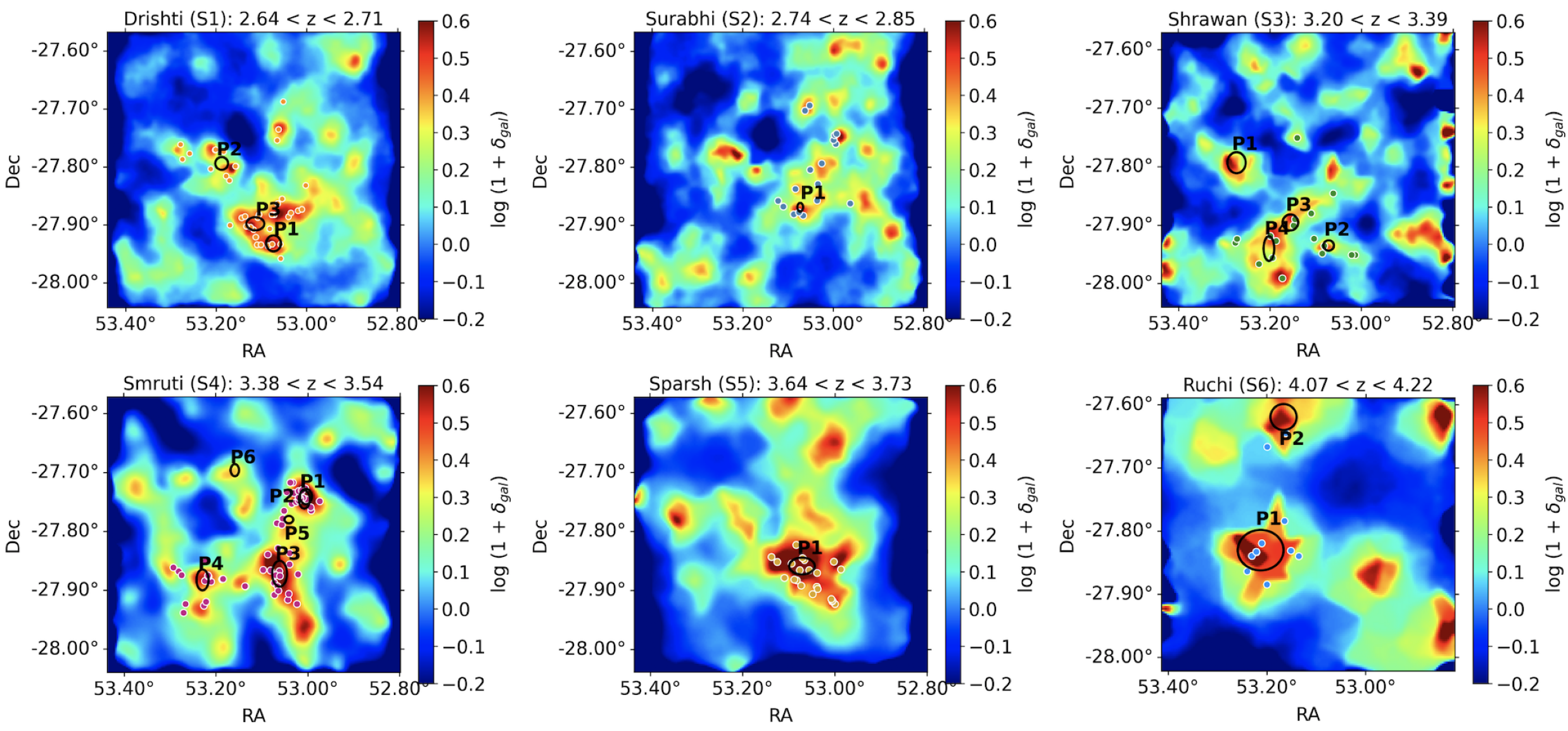
Figure 2: Projected Overdensity map of all six protostructures ($\sigma_{\delta}>2.5$) at $2.5<z<4.5$ presented in this study: The darker red colors present higher overdensity values and bluer colors present lower overdensity values. The overdense peaks ($\sigma_{\delta}>5$) with mass log($M/M_{\odot}>12$) are represented with black ellipses based on their $R_{x}$ and $R_{y}$ values from Table 1. The spectroscopic members of protostructures are presented using dots with the same protostructure specific color scheme as in the third panel of Figure 1.

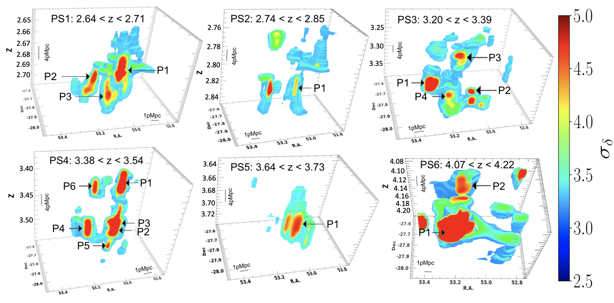
Figure 3: 3D Overdensity map of ECDFS in the redshift range all six protostructures: Red color shows higher overdensity and light blue shows lower overdensity. As a reminder, we use the term protostructure here and throughout the paper agnostically as we are unsure of their future fate. It can be seen that in some protostructures (e.g., protostructure 4 in lower left and protostructure 2 in the middle column of the upper panel), the overdense regions in red are connected through a relatively lower density bridge. There is also a wide range in the morphology and volume of the protostructures. The range of $\sigma_{\delta}$ is slightly larger (2.5-6.0 $\sigma_{\delta}$) for the highest redshift protostructure (PS6) than shown in the colorbar for a better visual representation of the structure.

Table 1: The properties of all six protostructures (S1-S6) and their corresponding overdense peaks (Pi) estimated using formulae described in Section 3.

ID	RA	DEC	z	$n_{sp}$a	<$\delta_{gal}$>b	V	$logM_{tot}$	SzFc	Rxd	Ryd	Rzd	Ez/xye	V${}_{corr}^{f}$	<$\delta_{gal}$>corrf
S1	53.0824	-27.8670	2.671	40	1.21	11292	14.9	0.09	-	-	-	-	-	-
P1_S1	53.0731	-27.9323	2.674	-	3.03	495	13.7	-	1.51	1.27	6.12	4.40	127	20.30
P2_S1	53.1876	-27.7943	2.694	-	2.36	297	13.4	-	1.49	1.16	7.54	5.69	59	23.11
P3_S1	53.1133	-27.8984	2.697	-	2.12	381	13.5	-	2.09	1.19	6.58	4.01	107	14.97
S2	52.9988	-27.8063	2.795	17	0.95	11251	14.8	0.09	-	-	-	-	-	-
P1_S2	53.0731	-27.8694	2.809	-	1.97	111	12.9	-	0.61	0.70	6.60	10.09	12	39.05
S3	53.1519	-27.9222	3.301	17	0.90	23634	15.1	0.12	-	-	-	-	-	-
P1_S3	53.2727	-27.7936	3.343	-	2.47	1683	14.1	-	2.05	1.85	8.53	4.36	386	19.01
P2_S3	53.0714	-27.9353	3.355	-	1.94	263	13.3	-	1.17	0.91	4.98	4.80	55	18.62
P3_S3	53.1552	-27.8959	3.242	-	1.98	629	13.7	-	1.73	1.38	7.06	4.54	139	17.66
P4_S3	53.2022	-27.9406	3.335	-	1.63	483	13.5	-	1.19	2.16	7.81	4.66	103	16.59
S4	53.0848	-27.8250	3.466	55	1.75	19854	15.1	0.18	-	-	-	-	-	-
P1_S4	53.0076	-27.7463	3.410	-	3.18	867	13.9	-	1.23	1.60	9.67	6.83	127	36.62
P2_S4	53.0042	-27.7411	3.479	-	3.86	650	13.8	-	1.34	1.37	10.03	7.40	88	44.90
P3_S4	53.0613	-27.8723	3.471	-	3.70	1740	14.3	-	1.68	2.30	9.44	4.75	367	27.11
P4_S4	53.2290	-27.8828	3.462	-	3.08	745	13.8	-	1.37	1.84	8.95	5.57	134	28.82
P5_S4	53.0412	-27.7804	3.530	-	3.93	141	13.2	-	0.99	0.66	5.25	6.36	22	38.66
P6_S4	53.1586	-27.6964	3.418	-	2.32	268	13.3	-	0.95	1.06	6.05	6.04	44	26.93
S5	53.0579	-27.8670	3.696	22	2.36	9032	14.8	0.20	-	-	-	-	-	-
P1_S5	53.0714	-27.8592	3.696	-	4.46	1201	14.1	-	2.96	1.52	7.17	3.20	375	20.22
S6	53.1876	-27.7991	4.144	11	1.15	42319	15.4	0.14	-	-	-	-	-	-
P1_S6	53.2124	-27.8306	4.150	-	2.48	11748	15.0	-	5.20	3.60	10.79	2.45	4789	10.51
P2_S6	53.1659	-27.6199	4.109	-	1.28	2552	14.2	-	2.96	2.31	8.99	3.41	748	11.68

The units of the columns of the table are - RA, DEC: [deg], V, Vcorr: [cMpc³], $M_{tot}$: [$M_{\odot}$], and Rx, Ry, and Rz: [cMpc]. The bias values used for the calculation of $M_{tot}$, $V_{corr}$, and <$\delta_{gal}$>_corr for the six protostructures, in order of increasing protostructure redshift, are 2.05, 2.10, 2.45, 2.55, 2.70, and 3.02, respectively, and are based on Chiang et al. (2013).

$a$: The number of $z_{spec}$ members in the protostructure satisfying stellar mass and IRAC magnitude cuts. We do not report the number of $z_{spec}$ members for peak regions $b$: The average galaxy overdensity in the region of interest as measured on the VMC maps $c$: Fraction of objects with photometric redshifts consistent with the protostructure that have secure spectroscopic redshifts $d$: Effective radius of the region of interest in the transverse and line of sight dimensions $e$: Elongation correction (see Cucciati et al. 2018) $f$: Corrected for elongation

4 Individual Protostructures and their properties

4.1 Protostructure 1: Drishti

Drishti is the lowest redshift protostructure reported here. It is located at $[\alpha_{J2000},\delta_{J2000}]=[53.0824,-27.8670$], spans $2.64<z<2.71$ and has a systemic redshift of $z$=2.671. It has a total mass of $10^{14.9}M_{\odot}$, an average $\sigma_{\delta}$ of 3.68, and occupies volume of 11292 cMpc³. It consists of three overdensity peaks, each with M${}_{tot}>10^{13.3}M_{\odot}$ as shown in Figure 2 and Figure 3. The southern-most peak P1_S1 is the largest and most massive of the three peaks. This protostructure was suggested by Guaita et al. (2020) based on the VANDELS observations. Their reported center of the highest density peak ($z=2.69$) is separated by $\sim 3.4$$\arcmin$ ($\sim$1.6 pMpc in projection) from P3_S1 at $z\sim 2.697$. However, they did not have any $z_{spec}$ members for this protostructure as opposed to the 40 $z_{spec}$ members in this work.

4.2 Protostructure 2: Surabhi

Surabhi is located at $[\alpha_{J2000},\delta_{J2000}]=[52.9988,-27.8063$] and $z$=2.795 ($2.74<z<2.85$). It has a total mass of $10^{14.8}M_{\odot}$, an average $\sigma_{\delta}$ of 3.29, and occupies a volume of $\sim 11251$ cMpc³. It has one overdensity peak with mass $>10^{12.8}M_{\odot}$, and two less massive peaks not reported here.

This protostructure may be related to three protoclusters at $z\sim 2.8$ in ECDFS identified in Zheng et al. (2016) based on the overdensity of LAEs. Guaita et al. (2020) also report a protostructure at $z\sim 2.8$ that could be related to this protostructure. Their protostructure is located $\sim$5$\arcmin$ ($\sim$2.4 pMpc in projection) from P1_S2 at $z\sim 2.809$. They report four $z_{spec}$ members as compared to 17 spectroscopic members in our work.

4.3 Protostructure 3: Shrawan

Shrawan is a massive protostructure situated at $[\alpha_{J2000},\delta_{J2000}]=[53.1519,-27.9222$] and redshift $z$=3.301 ($3.20<z<3.39$). It has a total mass of $10^{15.1}M_{\odot}$, an average $\sigma_{\delta}$ of 3.45, and it encompasses 23634 cMpc³. It contains four massive overdense peaks (each with $M_{tot}>10^{13.2}M_{\odot}$) as shown in Fig 2 and Fig 3. The northern-most peak, P1_S3, is the largest and most massive peak out of all four peaks. This protostructure has 17 spectroscopic member galaxies. A candidate overdensity, ‘CCPC-z32–003’ at $z=3.258$, is reported in Franck & McGaugh (2016) at a similar location, though with a “cluster probability” of 10%. This candidate is $\sim 0.13$ deg ($\sim$3.5 pMpc projected) from the nearest peak, P3_S3, at $z\sim 3.24$. Another candidate, ‘CCPC-z33–003’, is reported at $z=3.368$ is $\sim 0.16$ deg ($\sim$4.3 pMpc in projection) from the nearest redshift overdensity peak P2_S3 at $z\sim 3.355$. However, this candidate has a similarly low cluster probability of 10%.

4.4 Protostructure 4: Smruti

Smruti is a massive protostructure located at $[\alpha_{J2000},\delta_{J2000}]=[53.0848,-27.8250$] and $z$=3.466 ($3.38<z<3.54$). It has a mass of $M_{tot}=10^{15.1}M_{\odot}$, an average $\sigma_{\delta}$ of 4.05, and occupies a volume of 19854 cMpc³. It has six massive overdensity peaks (each with $M_{tot}>10^{13.1}M_{\odot}$) as shown in Fig 2 and Fig 3. The protostructure contains 55 spectroscopic member galaxies.

This existence of this protostructure was suggested by a few studies. An overdensity of galaxies at $z\sim 3.5$ was observed in the full redshift (both photometric and spectroscopic) distribution of galaxies in the GOODS-S/CDFS field in 3D-HST (Skelton et al., 2014), as well as observations from The FourStar Galaxy Evolution Survey (ZFOURGE) (Straatman et al., 2016). The overdensity was also alluded to in Guaita et al. (2020) as a protocluster candidate at $z=3.43$ identified in VANDELS with six spectroscopic members. It is $\sim$0.55$\arcmin$ ($\sim$0.24 pMpc in projection) away from the P1_S4, suggesting they are part of the same protostructure. Forrest et al. (2017) also detected an overdensity of Extreme [OIII]+H$\beta$ Emission Line Galaxies (EELGs) and Strong [OIII] Emission Line Galaxies (SELGs) at $z\sim 3.5$ that is $\sim 8.4$$\arcmin$ ($\sim$3.70 pMpc in projection) away from P3_S4. Franck & McGaugh (2016) report the candidate ‘CCPC-z34–002’ at $z=3.476$ with a cluster probability of 48%, which is $\sim$0.9$\arcmin$ ($\sim$0.40 pMpc in projection) away from P3_S4.

The peak P3_S4 also contains the most massive galaxy out of all ALMA-detected galaxies at $3<z<4$ in the GOODS-ALMA field (Ginolfi et al., 2017). Zhou et al. (2020) report that four optically dark galaxies detected in an ALMA continuum survey, reside in this protostructure, which suggests that considerable star formation activity is occurring in this protostructure. While the above studies appeared to detect parts of this protostructure, the extensive spectroscopic data and density mapping technique employed here interconnected and expanded on these detections.

4.5 Protostructure 5: Sparsh

Sparsh is located at $[\alpha_{J2000},\delta_{J2000}]=[53.0579,-27.8670$] and $z=3.696$ ($3.64<z<3.73$). It has a mass of $10^{14.8}M_{\odot}$, an average $\sigma_{\delta}$ of 3.48, and occupies a volume of 9032 cMpc³. It contains one massive overdensity peak, as well as two lower mass ($<$10¹³ $M_{\odot}$) peaks that are not reported here due to their small volume ($\sim$50 cMpc).

Hints of this protostructure were reported in Kang & Im (2009). They reported and overdensity at $z\sim 3.7$ that is $\sim 2.00$$\arcmin$ ($\sim$0.86 pMpc in projection) away from P1_S5. This study was followed by Kang & Im (2015), who also report on the same candidate with two $z_{spec}$ members. We find 22 spectroscopic member galaxies in this protostructure. Franck & McGaugh (2016) have two candidates that may correspond to this protostructure. The first is ‘CCPC-z36–002’ at $z=3.658$ with cluster probability 1%, which is $\sim 2.92\arcmin$ ($\sim 1.26$ pMpc in projection) away from P1_S5. The second is ‘CCPC-z37–001’ at $z=3.704$ with cluster probability 10%, which is $\sim 10.75$$\arcmin$ ($\sim$4.6 pMpc in projection) away from P1_S5.

4.6 Protostructure 6: Ruchi

Ruchi is the highest redshift protostructure reported here. It is located at $[\alpha_{J2000},\delta_{J2000}]=[53.1876,-27.7991$] and $z\sim 4.14$ ($4.07<z<4.22$). It is also the most massive protostructure, with a mass of $10^{15.4}M_{\odot}$, an average $\sigma_{\delta}$ of 5.15, and occupying the largest volume of our sample (42319 cMpc³). It has two overdensity peaks, each with mass more than $10^{14.0}M_{\odot}$ as shown in Fig 2 and Fig 3. We note that the precision of the mass estimates decreases at these high redshifts, due to relatively limited number of spectral redshifts and our inability to probe galaxies with lower luminosity and lower mass. There are 11 spectroscopic member galaxies in this protostructure. To our knowledge, this structure has not been reported in any other works.

5 Discussion

We report six massive protostructures (with masses greater than $10^{14.8}M_{\odot}$) in the ECDFS. While some hints of these structures were previously mentioned in other studies as described in the last section, it is only through our extensive spectroscopic and photometric samples, combined with the VMC mapping technique, that we have unequivocally confirmed the existence of these structures, mapped out their full extent, and measured their properties.

To contextualize these findings, we compare the observed number density of these protostructures with the predictions from a simulation based study that will be described in detail in an upcoming C3VO paper (Hung et al., in prep). Very briefly, we employ the GAlaxy Evolution and Assembly (GAEA) semi-analytic (SAM) model (Xie et al., 2017) applied to the dark matter merger trees of Millenium Simulation (Springel et al., 2005). A lightcone of radius 2.3 deg was generated from the Millenium simulation using a method similar to Zoldan et al. (2017). Mock observations are made of this lightcone that mimic the properties of the spectroscopic and photometric data in the ECDFS field, including spectroscopic redshift fraction and photo-$z$ statistics as a function of both redshift and apparent (IRAC1) magnitude. For each mock dataset, we perform identical VMC mapping to that performed on the real data (observations) and a structure finding technique is applied following the methodology described in Hung et al., in prep. From the full lightcone, we sampled 1000 iterations of fields with a volume equivalent to that of ECDFS over the range 2.5$<$$z$$<$4.5 taking care to avoid boundary effects. For each sampled volume, we counted the number of simulated protoclusters with similar masses to those of the protostructures detected in ECDFS taking into account completeness effects. Over all 1000 iterations we recover an expectation value of five protostructures with similar masses to those reported in this paper within an ECDFS-like volume from 2.5$<$$z$$<$4.5, with a 1$\sigma$ range of 3-7. These numbers are well consistent with the number of massive protostructures recovered in our observations.

Additionally, the sizes of all protostructures, with the possible exception of the $z\sim 4.144$ protostructure, are in agreement with the sizes predicted for protoclusters for the same mass and redshift based on simulations (Chiang et al., 2013, 2017; Muldrew et al., 2015; Contini et al., 2016, , Hung et al., in prep). For example, for simulated protoclusters in the mass and redshift range of the protostructures detailed in this work, Chiang et al. (2013) report a range of effective radii of $\sim 4.5$ cMpc - $\sim$ 10.5 cMpc, which is a size scale comparable to the protostructures identified here. However, we caution the reader that many differences exist in the methods used for identification of structure in observations and simulations, as well as differences in how structure sizes are calculated between simulations and observations. Some of the nuances associated with these comparisons will be detailed in an upcoming work (Hung et al., in prep). The range of volumes of all of our peaks at $z<4$ are comparable to the volume of the peaks of other C3VO structures at similar redshifts, e.g., Hyperion (Cucciati et al., 2018), Elentári (Forrest et al., 2023), and PCl J0227-0421 (Shen et al., 2021). The range of volumes for the highest redshift protostructure, Ruchi, at $z\sim 4.1$ is comparable to the range of volume of peaks in PCl J1001+0220 at $z\sim 4.57$ (Staab et. al., submitted).

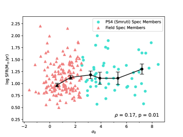
Figure 4: Relationship between SFR and overdensity ($\sigma_{\delta}$) for the spectroscopic members of the protostructure 4, i.e, Smruti ($\sigma_{\delta}>2.5$ and $3.38<z<3.54$), presented using filled turquoise circles and the spectroscopic members of a corresponding coeval field sample at $3.2<z<3.7$ and $\sigma_{\delta}<2.5$ presented using coral triangles. The black points show median values of the SFRs in a given $\sigma_{\delta}$ bin. The error bars show $1\sigma$ uncertainties in the median SFR values. The $\sigma_{\delta}$ bins for the black points are created such that all bins in the coeval field have approximately the same number of points and all bins for the protostructure members also have approximately the same number of points. A Spearman test for this data show a weak but statistically significant positive correlation between the SFR and environment.

To understand the impact of the dense protostructure environments on galaxy evolution, as a test case, we focus on Smruti at $z\sim 3.5$, as elevated star formation in this protostructure has been hinted at in previous works (e.g, Forrest et al., 2017; Ginolfi et al., 2017; Zhou et al., 2020). SFRs of the 55 $z_{spec}$ members of the protostructure ($\sigma_{\delta}>2.5$) as well as a corresponding coeval field sample at $3.2<z<3.7$ and $\sigma_{\delta}<2.5$ were used to investigate the relationship between SFR and environment in this protostructure as shown in Figure 4. A Spearman test is performed and returns a correlation coefficient of $\rho=0.17$ with $p=0.01$, which implies a weak but statistically significant positive correlation. This correlation is $\sim$30% stronger than that of the overall galaxy population at these redshifts (Lemaux et al., 2022). The positive correlation indicates rapid in situ stellar mass growth in the dense environments of such high-redshift protostructures, which is potentially necessary for forming the massive galaxies observed in clusters in the nearby universe (Baldry et al., 2006; Bamford et al., 2009; Calvi et al., 2013). This enhanced star formation in protostructures at high redshift is also in agreement with the results from some simulation-based studies (e.g., Chiang et al., 2017) and observations-based studies (e.g, Greenslade et al., 2018; Lemaux et al., 2022). We will present a detailed study on this relation, as well as other galaxy properties, in all of the protostructures reported here, as well as lower mass systems, in a follow-up paper (E. Shah et. al., in prep).

6 Summary

We identify and present six spectroscopically-confirmed massive ($M_{tot}>10^{14.8}M_{\odot}$) protostructures at $2.5<z<4.5$ in the ECDFS field. These structures are identified by applying an overdensity-measurement technique on the publicly available extensive spectroscopic and photometric observations as well as targeted spectral observations in the ECDFS field from the C3VO survey. We calculate the volume, mass, and average overdensities of the protostructures, as well as other associated quantities. One of these protostructures, named Smruti, is a large complex protostructure at $z\sim 3.47$ containing six overdense ($\sigma_{\delta}>5$) peaks and 55 spectroscopic members. Its member galaxies show a statistically significant correlation between the SFR and environment density. This protostructure, as well as another protostructure at $z$$\sim$3.3, dubbed Shrawan, are very massive ($M\sim 10^{15.15}M_{\odot}$) and each contains $\geq 4$ overdense peaks. The remaining protostructures at $z$$<$4 are slightly less massive (10^14.8-14.9 $M_{\odot}$) and contain fewer peaks. The highest redshift protostructure reported here ($z$$\sim$4.14), dubbed Ruchi, contains 11 spectroscopic members. The number density, masses, and sizes of these protostructures are broadly in agreement with the prediction of these properties of protoclusters in simulations (Chiang et al., 2013, 2017; Muldrew et al., 2015; Contini et al., 2016, , Hung et al., in prep). These protostructures span wide ranges of complexity, masses, volume, and redshift and will be used in a companion paper (Shah et al. in prep) to study the effect of dense environments on star formation and nuclear activity at high redshift.

7 Data Availability

The data used this study would be shared based on a reasonable request to the corresponding author.

References

- Abadi et al. (1999) Abadi M. G., Moore B., Bower R. G., 1999, MNRAS, 308, 947
- Alonso et al. (2012) Alonso S., Mesa V., Padilla N., Lambas D. G., 2012, A&A, 539, A46
- Arnouts et al. (1999) Arnouts S., Cristiani S., Moscardini L., Matarrese S., Lucchin F., Fontana A., Giallongo E., 1999, MNRAS, 310, 540
- Baldry et al. (2006) Baldry I. K., Balogh M. L., Bower R. G., Glazebrook K., Nichol R. C., Bamford S. P., Budavari T., 2006, MNRAS, 373, 469
- Bamford et al. (2009) Bamford S. P., et al., 2009, MNRAS, 393, 1324
- Bassini et al. (2020) Bassini L., et al., 2020, A&A, 642, A37
- Bekki (2009) Bekki K., 2009, MNRAS, 399, 2221
- Bekki et al. (2002) Bekki K., Couch W. J., Shioya Y., 2002, ApJ, 577, 651
- Birkin et al. (2021) Birkin J. E., et al., 2021, MNRAS, 501, 3926
- Boselli et al. (2022) Boselli A., Fossati M., Sun M., 2022, A&ARv, 30, 3
- Brienza et al. (2023) Brienza M., et al., 2023, A&A, 672, A179
- Calvi et al. (2013) Calvi R., Poggianti B. M., Vulcani B., Fasano G., 2013, MNRAS, 432, 3141
- Cannarozzo et al. (2023) Cannarozzo C., et al., 2023, MNRAS, 520, 5651
- Cardamone et al. (2010) Cardamone C. N., et al., 2010, ApJS, 189, 270
- Casey et al. (2015) Casey C. M., et al., 2015, ApJ, 808, L33
- Chabrier (2003) Chabrier G., 2003, PASP, 115, 763
- Chartab et al. (2020) Chartab N., et al., 2020, ApJ, 890, 7
- Chiang et al. (2013) Chiang Y.-K., Overzier R., Gebhardt K., 2013, ApJ, 779, 127
- Chiang et al. (2017) Chiang Y.-K., Overzier R. A., Gebhardt K., Henriques B., 2017, ApJ, 844, L23
- Clements et al. (2014) Clements D. L., et al., 2014, MNRAS, 439, 1193
- Contini et al. (2016) Contini E., De Lucia G., Hatch N., Borgani S., Kang X., 2016, MNRAS, 456, 1924
- Cooper et al. (2012) Cooper M. C., et al., 2012, MNRAS, 425, 2116
- Cowie & Songaila (1977) Cowie L. L., Songaila A., 1977, Nature, 266, 501
- Cucciati et al. (2014) Cucciati O., et al., 2014, A&A, 570, A16
- Cucciati et al. (2018) Cucciati O., et al., 2018, A&A, 619, A49
- D’Amato et al. (2020) D’Amato Q., et al., 2020, A&A, 641, L6
- Dahlen et al. (2013) Dahlen T., et al., 2013, ApJ, 775, 93
- Damen et al. (2011) Damen M., et al., 2011, ApJ, 727, 1
- Di Mascolo et al. (2023) Di Mascolo L., et al., 2023, Nature, 615, 809
- Eisenstein et al. (2023) Eisenstein D. J., et al., 2023, arXiv e-prints, p. arXiv:2306.02465
- Faber et al. (2003) Faber S. M., et al., 2003, in Iye M., Moorwood A. F. M., eds, Society of Photo-Optical Instrumentation Engineers (SPIE) Conference Series Vol. 4841, Instrument Design and Performance for Optical/Infrared Ground-based Telescopes. pp 1657–1669, doi:10.1117/12.460346
- Forrest et al. (2017) Forrest B., et al., 2017, ApJ, 838, L12
- Forrest et al. (2023) Forrest B., et al., 2023, MNRAS, 526, L56
- Franck & McGaugh (2016) Franck J. R., McGaugh S. S., 2016, ApJ, 817, 158
- Gawiser et al. (2006) Gawiser E., et al., 2006, ApJS, 162, 1
- Giacconi et al. (2002) Giacconi R., et al., 2002, ApJS, 139, 369
- Ginolfi et al. (2017) Ginolfi M., et al., 2017, MNRAS, 468, 3468
- Grazian et al. (2006) Grazian A., et al., 2006, A&A, 449, 951
- Greenslade et al. (2018) Greenslade J., et al., 2018, MNRAS, 476, 3336
- Grogin et al. (2011) Grogin N. A., et al., 2011, ApJS, 197, 35
- Guaita et al. (2020) Guaita L., et al., 2020, A&A, 640, A107
- Guo et al. (2013) Guo Y., et al., 2013, ApJS, 207, 24
- Hatch et al. (2014) Hatch N. A., et al., 2014, MNRAS, 445, 280
- Hildebrandt et al. (2006) Hildebrandt H., et al., 2006, A&A, 452, 1121
- Hsu et al. (2014) Hsu L.-T., et al., 2014, ApJ, 796, 60
- Hung et al. (2016) Hung C.-L., et al., 2016, ApJ, 826, 130
- Hung et al. (2020) Hung D., et al., 2020, MNRAS, 491, 5524
- Husband et al. (2013) Husband K., Bremer M. N., Stanway E. R., Davies L. J. M., Lehnert M. D., Douglas L. S., 2013, MNRAS, 432, 2869
- Ilbert et al. (2006) Ilbert O., et al., 2006, A&A, 457, 841
- Ito et al. (2020) Ito K., et al., 2020, ApJ, 899, 5
- Jiang et al. (2018) Jiang L., et al., 2018, Nature Astronomy, 2, 962
- Kang & Im (2009) Kang E., Im M., 2009, ApJ, 691, L33
- Kang & Im (2015) Kang E., Im M., 2015, Journal of Korean Astronomical Society, 48, 21
- Karouzos et al. (2014) Karouzos M., et al., 2014, ApJ, 797, 26
- Kaviraj et al. (2008) Kaviraj S., et al., 2008, MNRAS, 388, 67
- Koekemoer et al. (2011) Koekemoer A. M., et al., 2011, ApJS, 197, 36
- Kriek et al. (2015) Kriek M., et al., 2015, ApJS, 218, 15
- Larson et al. (1980) Larson R. B., Tinsley B. M., Caldwell C. N., 1980, ApJ, 237, 692
- Le Fèvre et al. (2003) Le Fèvre O., et al., 2003, in Iye M., Moorwood A. F. M., eds, Society of Photo-Optical Instrumentation Engineers (SPIE) Conference Series Vol. 4841, Instrument Design and Performance for Optical/Infrared Ground-based Telescopes. pp 1670–1681, doi:10.1117/12.460959
- Le Fèvre et al. (2004) Le Fèvre O., et al., 2004, A&A, 428, 1043
- Le Fèvre et al. (2013) Le Fèvre O., et al., 2013, A&A, 559, A14
- Le Fèvre et al. (2015) Le Fèvre O., et al., 2015, A&A, 576, A79
- Lehmer et al. (2005) Lehmer B. D., et al., 2005, ApJS, 161, 21
- Lemaux et al. (2014) Lemaux B. C., et al., 2014, A&A, 572, A41
- Lemaux et al. (2017) Lemaux B. C., Tomczak A. R., Lubin L. M., Wu P. F., Gal R. R., Rumbaugh N., Kocevski D. D., Squires G. K., 2017, MNRAS, 472, 419
- Lemaux et al. (2018) Lemaux B. C., et al., 2018, A&A, 615, A77
- Lemaux et al. (2019) Lemaux B. C., et al., 2019, MNRAS, 490, 1231
- Lemaux et al. (2022) Lemaux B. C., et al., 2022, A&A, 662, A33
- Luo et al. (2010) Luo B., et al., 2010, ApJS, 187, 560
- Marchi et al. (2018) Marchi F., et al., 2018, A&A, 614, A11
- McConachie et al. (2022) McConachie I., et al., 2022, ApJ, 926, 37
- McLean et al. (2010) McLean I. S., et al., 2010, in McLean I. S., Ramsay S. K., Takami H., eds, Society of Photo-Optical Instrumentation Engineers (SPIE) Conference Series Vol. 7735, Ground-based and Airborne Instrumentation for Astronomy III. p. 77351E, doi:10.1117/12.856715
- McLean et al. (2012) McLean I. S., et al., 2012, in McLean I. S., Ramsay S. K., Takami H., eds, Society of Photo-Optical Instrumentation Engineers (SPIE) Conference Series Vol. 8446, Ground-based and Airborne Instrumentation for Astronomy IV. p. 84460J, doi:10.1117/12.924794
- McLure et al. (2018) McLure R. J., et al., 2018, MNRAS, 479, 25
- McNab et al. (2021) McNab K., et al., 2021, MNRAS, 508, 157
- Mei et al. (2023) Mei S., et al., 2023, A&A, 670, A58
- Miller et al. (2018) Miller T. B., et al., 2018, Nature, 556, 469
- Momcheva et al. (2016) Momcheva I. G., et al., 2016, ApJS, 225, 27
- Moore et al. (1996) Moore B., Katz N., Lake G., Dressler A., Oemler A., 1996, Nature, 379, 613
- Moore et al. (1998) Moore B., Lake G., Katz N., 1998, ApJ, 495, 139
- Moy et al. (2003) Moy E., Barmby P., Rigopoulou D., Huang J. S., Willner S. P., Fazio G. G., 2003, A&A, 403, 493
- Muldrew et al. (2015) Muldrew S. I., Hatch N. A., Cooke E. A., 2015, MNRAS, 452, 2528
- Newman et al. (2013) Newman J. A., et al., 2013, ApJS, 208, 5
- Nulsen (1982) Nulsen P. E. J., 1982, MNRAS, 198, 1007
- Oke & Gunn (1983) Oke J. B., Gunn J. E., 1983, ApJ, 266, 713
- Old et al. (2020) Old L. J., et al., 2020, MNRAS, 493, 5987
- Overzier (2016) Overzier R. A., 2016, A&ARv, 24, 14
- Peluso et al. (2022) Peluso G., et al., 2022, ApJ, 927, 130
- Pentericci et al. (2018) Pentericci L., et al., 2018, A&A, 616, A174
- Shen et al. (2021) Shen L., et al., 2021, ApJ, 912, 60
- Shi et al. (2019) Shi K., et al., 2019, ApJ, 879, 9
- Skelton et al. (2014) Skelton R. E., et al., 2014, ApJS, 214, 24
- Song et al. (2016) Song H., Park C., Lietzen H., Einasto M., 2016, ApJ, 827, 104
- Springel et al. (2005) Springel V., et al., 2005, Nature, 435, 629
- Straatman et al. (2016) Straatman C. M. S., et al., 2016, ApJ, 830, 51
- Tasca et al. (2015) Tasca L. A. M., et al., 2015, A&A, 581, A54
- Tomczak et al. (2017) Tomczak A. R., et al., 2017, MNRAS, 472, 3512
- Tomczak et al. (2019) Tomczak A. R., et al., 2019, MNRAS, 484, 4695
- Toshikawa et al. (2023) Toshikawa J., et al., 2023, MNRAS,
- Uchiyama et al. (2018) Uchiyama H., et al., 2018, PASJ, 70, S32
- Virani et al. (2006) Virani S. N., Treister E., Urry C. M., Gawiser E., 2006, AJ, 131, 2373
- Wuyts et al. (2008) Wuyts S., Labbé I., Förster Schreiber N. M., Franx M., Rudnick G., Brammer G. B., van Dokkum P. G., 2008, ApJ, 682, 985
- Xie et al. (2017) Xie L., De Lucia G., Hirschmann M., Fontanot F., Zoldan A., 2017, MNRAS, 469, 968
- Xue et al. (2016) Xue Y. Q., Luo B., Brandt W. N., Alexander D. M., Bauer F. E., Lehmer B. D., Yang G., 2016, ApJS, 224, 15
- Zavala et al. (2019) Zavala J. A., et al., 2019, ApJ, 887, 183
- Zheng et al. (2004) Zheng W., et al., 2004, ApJS, 155, 73
- Zheng et al. (2016) Zheng Z.-Y., Malhotra S., Rhoads J. E., Finkelstein S. L., Wang J.-X., Jiang C.-Y., Cai Z., 2016, ApJS, 226, 23
- Zhou et al. (2020) Zhou L., et al., 2020, A&A, 642, A155
- Zoldan et al. (2017) Zoldan A., De Lucia G., Xie L., Fontanot F., Hirschmann M., 2017, MNRAS, 465, 2236
- van den Bosch et al. (2008) van den Bosch F. C., Aquino D., Yang X., Mo H. J., Pasquali A., McIntosh D. H., Weinmann S. M., Kang X., 2008, MNRAS, 387, 79
- van der Burg et al. (2020) van der Burg R. F. J., et al., 2020, A&A, 638, A112