Massive black hole binaries in LISA: constraining cosmological parameters at high redshifts

Abstract

One of the primary scientific objectives of the Laser Interferometer Space Antenna (LISA) is to probe the expansion of the Universe using gravitational wave observations. Indeed, as gravitational waves from the coalescence of a massive black hole binary (MBHB) carry direct information of the luminosity distances, an accompanying electromagnetic (EM) counterpart can be used to determine the redshift. This method of bright sirens enables one to build a gravitational Hubble diagram to high redshift when applied to LISA. In this work, we forecast the ability of LISA-detected MBHB bright sirens to constrain cosmological models. As the expected EM emission from MBHBs can be detected up to redshift $z\sim 7$ with future astronomical facilities, we focus on the ability of LISA to constrain the expansion of the Universe at $z\sim 2-3$, a poorly charted epoch in cosmography. We find that a model-independent approach to cosmology based on a spline interpolation of the luminosity distance-redshift relation, can constrain the Hubble parameter at $z\sim 2-3$ with a relative precision of at least $10\%$.

I Introduction

In the next decade, the Laser Interferometer Space Antenna (LISA) Amaro-Seoane et al. (2017) will observe gravitational waves (GWs) from the coalescence of massive black hole binaries (MBHBs) of mass $10^{4}-10^{7}{\,\rm M}_{\odot}$ at redshifts up to $z\sim 20$.

For nearly 40 years, these systems have been considered as the key to a method that can shed light on the cosmic expansion history of our Universe Schutz (1986); Auclair et al. (2022). Indeed, a coalescing binary system can be considered as a standard siren because the final burst of GWs carries direct information of the luminosity distance of the source. The GW signal is degenerate in the redshift, however, meaning that additional information is required to infer the distance-redshift relationship.

If an electromagnetic (EM) counterpart is associated with the coalescence, the redshift may be determined with spectroscopic or photometric follow-up observations Tamanini et al. (2016); Holz and Hughes (2005); Dalal et al. (2006); Nissanke et al. (2010); Del Pozzo (2012); Abbott et al. (2017a); Mangiagli et al. (2022); D’Orazio and Charisi (2023). This approach to constructing a standard-siren distance-redshift relationship is usually referred to in the literature as the method of bright sirens. In the absence of an EM counterpart, the redshift may be estimated probabilistically by cross-correlating the region hosting the GW merger with galaxy catalogs Petiteau et al. (2011); Del Pozzo et al. (2018); Kyutoku and Seto (2017a); Muttoni et al. (2022); Laghi et al. (2021); Zhu et al. (2022); Dalang and Baker (2023). This approach is referred to as the method of dark sirens. Finally, the redshift may also be inferred from the detected mass distribution of the source. Due to cosmic expansion, the gravitational waveform determines the product $M(1+z)$ where $M$ is the intrinsic, rest-frame mass parameter. Assuming a parametrized functional form for the intrinsic mass distribution, the cosmological parameters can be constrained together with the parameters describing the mass distribution The LIGO Scientific Collaboration et al. (2021a); Ezquiaga and Holz (2022). This approach has been recently named the method of spectral sirens. The dark and spectral siren approaches can be combined in a single inference methodology where both information on the intrinsic distribution of sources and cross-correlation with galaxy catalogs provide stringier cosmological constraints Gray et al. (2023); Mastrogiovanni et al. (2023); Leyde et al. (2023). Further approaches have been proposed to test cosmology with GWs, for example, by exploiting the cross-correlation of the weak lensing of both GWs and galaxy fields Balaudo et al. (2022); Mukherjee et al. (2021), prior knowledge either of the equation of state of neutron stars Messenger and Read (2012); Chatterjee et al. (2021) or of the merger rate evolution of GW sources Ding et al. (2019); Ye and Fishbach (2021).

A new, independent method to determine the distance-redshift relationship would provide valuable information about the nature of our Universe. The standard $\Lambda$CDM model provides a good fit to the bulk of cosmological data. However, in recent years, several tensions between late- and early-Universe measurements have arisen. The most famous one is the Hubble constant $H_{0}$ tension wherein early-time measurements from the Cosmic Microwave Background (CMB) report a value of $H_{0}\sim 67\,\rm km/s/Mpc$ Planck Collaboration et al. (2020) and late-time measurements from supernovae (SNe) obtain $H_{0}\sim 72\,\rm km/s/Mpc$ Riess et al. (2021). (See also Di Valentino et al. (2021); Abdalla et al. (2022); Perivolaropoulos and Skara (2022) and reference therein for recent reviews on the topic.) Whether these tensions are due to systematics in the different measurements and datasets or are the hints of new physics is a pressing, open question.

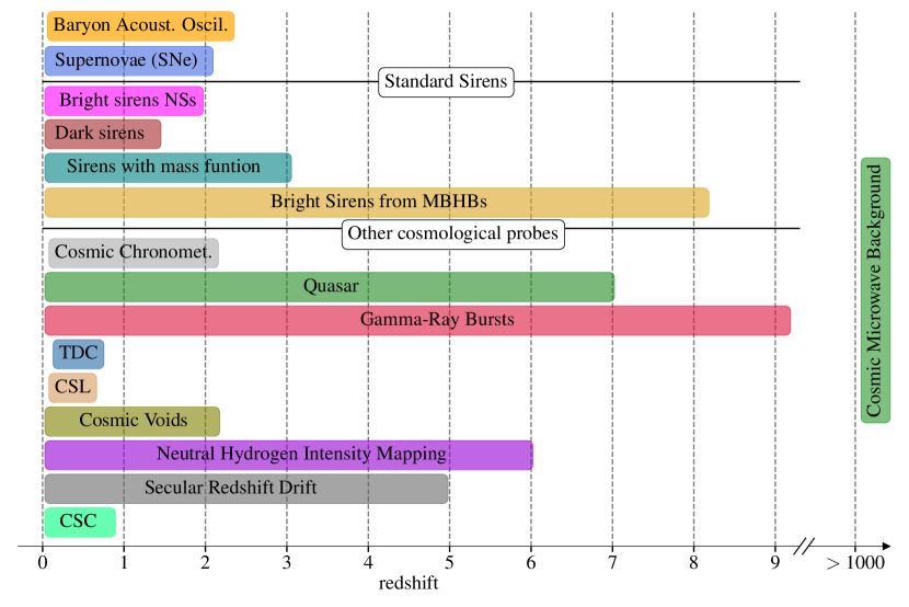
Figure 1: Redshift range covered by several cosmological probes. On the right and on the top, the three main cosmological probes, i.e. CMB, BAO and SNe. In the middle, the standard sirens forecasts with different approaches for future 3G detectors and LISA. In the bottom part, other emerging cosmological probes. The acronyms stand for cosmic chronometers (‘Cosmic Chronomet.’), time delay cosmography (TDC), cluster strong lensing (CSL) and clustering of standard candles (CSC). Bright sirens from MBHBs can probed the expansion of the Universe up to $z\sim 8$ where few other cosmological probes are available. We refer to Moresco et al. (2022) for more details on each of the techniques listed in the plot.

In Fig. 1 we report the redshift range covered by different cosmological probes (see also Fig. 52 in Moresco et al. (2022) for a similar plot). The three main measurements in the literature are the CMB at early-time and SNe and BAO at late-time. However, while the former is at $z>1000$, the latters can test the expansion up to $z\sim 2$ Riess et al. (2018) and $z\sim 2.5$ Addison et al. (2018), respectively.

Moving to standard sirens, current ground-based detectors are expected to detect NS-NS and NS-BH mergers up to $z\sim 0.1$ Colombo et al. (2022). Third-generation ground-based detectors as Einstein Telescope (ET) Punturo et al. (2010) and Cosmic Explorer (CE) Abbott et al. (2017b), together with EM facilities as Fermi Meegan et al. (2009) and Theseus Amati et al. (2018), should be able to detect the GW signal and the EM emission up to $z\sim 2.5$ in X-ray and up to $z\sim 3$ in $\gamma$-band Ronchini et al. (2022). The dark sirens approach can be, in principle, applied to any type of standard sirens, i.e. compact object binaries in ground-based interferometers or in the high-frequency portion of LISA band Del Pozzo et al. (2018); Kyutoku and Seto (2017b); Muttoni et al. (2022) and extreme-mass ratio inspiral (EMRIs) MacLeod and Hogan (2008); Laghi et al. (2021); Liu et al. (2023). However, independently from the type of source, this technique is limited to $z\sim 1$-1.5 by the completeness of the galaxy catalogs. Concerning spectral sirens, current detectors are limited at $z\sim 1.5$ at design sensitivity Taylor et al. (2012); Leyde et al. (2022); Mancarella et al. (2022); Leandro et al. (2022), but ET and CE can potentially expand this approach up to $z\sim 3$. The peak of the star formation rate is at $z\sim 2-3$, meaning that the number of BHs and NSs will decrease quickly at higher redshifts Santoliquido et al. (2021) and BHBs will not provide strong constraints on $H(z)$ at $z\gtrsim 2$ (see Fig. 1 in Ezquiaga and Holz (2022)). MBHs can also be used as spectral sirens even if, at the moment, we do not expect any particular feature in their mass distribution and a consistent study is still missing. Finally, the detection of the GW signal from a MBHB merger together with the identification of the host galaxy, might probe the expansion of the Universe up to $z\sim 8$ Tamanini et al. (2016); Mangiagli et al. (2022); Speri et al. (2021), depending on the astrophysical model assumed. However, although MBHBs may become interesting sources to test alternative cosmological models at high-redshift Caprini and Tamanini (2016); Cai et al. (2017); Corman et al. (2022, 2021); Belgacem et al. (2019), there are large uncertainties on the expected rates of MBHB mergers (see Sec. 2.4.2 in Amaro-Seoane et al. (2022)), on the modeling of the EM counterpart and on the possibility to identify the host galaxy at high redshift.

In the lower part of the plot, we show other cosmological probes that have been exploited in the recent years. Here we describe briefly the probes at $z>3$ and refer the interested reader to Moresco et al. (2022) for a complete review.

Quasar have been proposed as standardizable candles, exploiting the non linear relation between the X-ray and UV luminosities (Risaliti and Lusso (2019) and reference therein). This relation should represent an universal mechanism taking place in quasars and their emission can be detected up to $z\sim 7$. However the selection of the samples is affected by observational issues, leading to an intrinsic dispersion of $0.2$ dex (even if this value reduces to $0.12$ with high-quality data Sacchi et al. (2022)), and the majority of quasars is located at $z<4$.

Similarly, gamma-ray bursts (GRBs) can be promoted to cosmological probes exploiting correlations between rest- and observer-frame quantities, as the relation between the intrinsic peak energy and the total radiated energy Amati et al. (2002). GRBs can be detected up to very high redshift $z\sim 9$-10 and, emitting in $\gamma$ and hard X-ray band, they are not affected by dust absorption. However the correlations can not be calibrated in a cosmology-independent way due to the lack of low-redshift events. Therefore the parameters describing the empirical relations have to be fitted together with the cosmological parameters Amati and Della Valle (2013) or calibrated with lower redshift standard candles, as SNe Demianski et al. (2017).

Neutral hydrogen intensity mapping consists in exploiting the $21\,\rm cm$ emission to map the large-scale structures Kovetz et al. (2019). Even if the single galaxies are not resolved, the neutral hydrogen follows the matter density fluctuations, providing information of the Universe evolution. This emission can be detected up to very high redshift but there might be contamination from other sources.

The secular redshift shift consists in measuring the variation in redshift due to an expanding Universe Loeb (1998). Any type of redshift indicator can be used (absorption/emission lines and feature in the spectrum) and the approach is completely cosmological model-independent. However it require long observing time and it might not be as accurate as other cosmological probes.

Standard sirens represent a new cosmological probe to test the expansion of the Universe. Motivated by the redshift range from Fig. 1, in this work we examine the potential of MBHBs as bright sirens to constrain the cosmic evolution of the Universe at intermediate redshifts. In particular, current knowledge of the properties of MBHBs suggests that we may be able to probe the expansion across redshifts $2\lesssim z\lesssim 8$, a territory that is still poorly explored in modern cosmology.

We built this paper on the previous work done in Mangiagli et al. 2022 (hereafter ‘M22’) where we explored the number of MBHBs mergers emitting a detectable EM counterpart under different astrophysical models and EM configurations. Here we focus on the subset of EM counterparts (EMcps), i.e. systems with :

1. GW signal-to-noise ratio (SNR) above 10;

2. Detectable EM emission;

3. Sufficiently accurate sky-localization, depending on the EM telescopes considered (see Mangiagli et al. (2022) for more details).

We assume to be able to identify the host galaxy of EMcps and to get an independent measurement of the redshift. In other words, EMcps are standard sirens, i.e. systems that can be used to test the expansion of the Universe. For each astrophysical population, we build 100 realisations to perform cosmological tests. We divide the analysis in two branches: the first focuses on local Universe quantities such as the local Hubble constant, $\Omega_{m}$ or late-time dark energy models while the second explores LISA capabilities to constrain $H(z)$ at $z\gtrsim 2$ using various strategies, both model-dependent and -independent.

The paper is organised as follows. In Sec. II we review the results of M22. In Sec. III we introduce some useful notions in cosmology and we present the models we tested in this work. The catalogues of MBHBs are constructed in Sec. IV and the likelihood is formulated in Sec. V. In Sec. VI we present the analysis setup and discuss some caveats. In Sec. VII we report our main results. In Sec. VIII we conclude with some final remarks and comments. In Appendix A we check that the number of realisations are sufficient to provide solid results. In Appendix B we assess the Gaussianity of the luminosity distance posterior distributions. In Appendix C we discuss a test we adopted to determine informative realisations. In Appendix D we derive a redshift where the correlation between the Hubble parameter and $\Omega_{m}$ is minimum.

II Review of M22

In this section we briefly summarise the main results of M22. We build our methodology on the previous work done by Tamanini et al. (2016) with some major improvements. Since this work is a follow-up of M22, here we limit to summarise the most important results and refer the interested readers to the original paper.

There are still large uncertainties on the populations of MBHBs that LISA will observe, mostly due to the lack of observational evidences. Therefore we have to rely on simulations. In the past years, semi-analytical models (SAMs) have established as one of the possible approach to predict the population of merging MBHBs. In this work we adopt the SAM developed in Barausse (2012) (with contributions from Sesana et al. (2014); Antonini et al. (2015a, b)) to track the evolution of MBHs across cosmic time. We consider three different astrophysical models:

1. Pop3: a model where MBHs grow from light seeds BHs that are the remnant of young metal-poor Pop3 stars. This model takes into account the delay between the galaxy merger and the MBHB merger;

2. Q3d: in this case, MBHs originate from the collapse of proto-galactic disks at $10^{4}-10^{6}{\,\rm M}_{\odot}$. Time-delays between mergers are included;

3. Q3nd: a heavy-seed scenario, similar to Q3d, but without merger time-delays, leading to an increase number of MBHB mergers.

The three population models above yield three qualitatively different catalogs of MBHB mergers across cosmic time. Among these, we are interested in the MBHB mergers producing an EM counterpart.

Even larger uncertainties affect the EM emission from MBHBs. Even if few binary-AGN candidates at sub-parsec separation have been reported (see Part II in De Rosa et al. (2020) for a recent review), these systems are still far from merger in the LISA frequency band and more massive than the ones LISA will be able to detect. The behaviour of gas in a rapidly changing space-time is yet unclear so we have to rely again on simulations. During the inspiral phase, General Relativity MagnetoHydroDynamic (GRMHD) simulations showed that the binary excavate a cavity in the circumbinary disks and streams of gas flow from the inner edge to form minidisks around each BHs Bowen et al. (2018); Gold et al. (2014); Noble et al. (2021); Combi et al. (2022); Franchini et al. (2022); Cattorini et al. (2022). While UV photons are produced by the inner edge of the circumbinary disk, a large amount of X-ray radiation is emitted by the minidisks Tang et al. (2018); d’Ascoli et al. (2018). The motion of the binary is expected to imprint a modulation in the EM emission Dal Canton et al. (2019). If the binary is already ‘on’ years before the merger, the modulation might appear in optical and, possibly, it can be detected with surveys as LSST Ivezić et al. (2019). In the last phase of the inspiral, the modulation can be instead detected in X-ray with future telescopes, such as the Advanced Telescope for High ENergy Astrophysics (Athena) Nandra et al. (2013); Piro et al. (2023).

During or after the merger, flare or jet emissions are expected at different wavelengths and on timescales of weeks or months Milosavljevic and Phinney (2005); Fontecilla et al. (2017); Yuan et al. (2021). Additional transient features might be produced by a re-brightening of the accretion disk or by internal shocks in the gas, adjusting to the new gravitational potential Rossi et al. (2010).

To test the expansion on the Universe with bright MBHBs sirens, we get the luminosity distance estimate from the GW signal and the redshift from the EM counterpart. As in M22, if the source is sufficiently bright in optical, its redshift can be determined with the Vera C. Rubin Observatory Ivezić et al. (2019); abo . Otherwise, the host galaxy can be identified in radio with the Square Kilometre Array (SKA) Dewdney et al. (2009) telescope or in X-ray with Athena Piro et al. (2022) . The source redshift can be subsequently determined with photometric or spectroscopic observations performed, for example, with the Extremely Large Telescope (ELT) E-ELT .

In M22, we defined a GW event with EM counterpart (EMcp for the rest of the paper) as a system whose EM counterpart can be detected by any of our strategies and whose sky localization is sufficiently accurate to fall inside the aforementioned telescopes field of view (FOV). Therefore, these sources represent the subset of MBHB systems for which we have both the luminosity distance and the redshift measurements.

The rate of EMcps changes significantly depending on the processes responsible for the production of the EM counterpart (i.e. the accretion rate or the jet opening angle for the radio emission), on the assumptions of the environment surrounding the MBHBs (i.e. the AGN obscuration) and on the sky localization provided by LISA. In order to simplify the presentation of results, in M22 we considered two models, labelled as ‘maximising’ and ‘minimising’. The two main differences between these models were that in the former there was no AGN obscuration and the radio flare emission was isotropic while, in the latter, we included the AGN obscuration and the radio flare emission was collimated with an opening angle of $\sim 30^{\circ}$. In Tab. 1 we report the average number of EMcps for each model, assuming 4yr of observations. The ‘maximising’ model predicts on average between $\sim 7$ and $\sim 20$ EMcps in 4 yr, depending on the astrophysical population, while in the ‘minimising’ one we expect $\sim 2-3$ EMcps. The AGN obscuration and the collimated jet emission are the two main factors that drastically reduce the number of EMcps.

Standard siren cosmology is one of the LISA science objectives that strongly depends on the number of sources and on the mission time Auclair et al. (2022). In this study, we consider only the ‘maximising’ case and not the ‘minimising’ one, due to its limited number of EMcps. If the ‘minimising’ case will result to be the one closer to reality, the cosmology science case with bright MBHBs will be undermined if LISA will operate for only 4 yr. However we note that in 10yr the heavy models (Q3d and Q3nd) in the minimising case predict $\sim 3.3\times 10/4\sim 8.2$ EMcps which are close to the number of EMcps in the Pop3 model in the ‘maximising’ case but in 4yr.

Table 1: Average number of EMcps in 4yr for ‘maximising’ and ‘minimising’ case.

(in 4yr)	Maximising	Minimising
Pop3	6.4	1.6
Q3d	14.8	3.3
Q3nd	20.7	3.5

III Cosmological models

In the standard Friedmann-Lemaître-Robertson-Walker (FLRW) formalism, we can define the universe metric as Dodelson (2003); Piattella (2018)

$$ds^{2}=-c^{2}dt^{2}+a^{2}(t)\left(\frac{dr}{1-Kr^{2}}+r^{2}d\Omega\right)$$ (1)

with $K=0,-1,+1$, $a(t)$ the scale factor and $c$ the light speed. From the FLRW, we can derive the Friedmann equations as

$$H^{2}=\frac{8\pi G}{3}\rho-\frac{Kc^{2}}{a^{2}}$$ (2)

$$\frac{\ddot{a}}{a}=\frac{-4\pi G}{3}\left(\rho+\frac{3P}{c^{2}}\right)$$ (3)

where $H=(da/dt)/a=\dot{a}/a$ is the Hubble rate, $G$ the gravitational constant and $\rho$ and $P$ are the sum of the energy densities of all the components of our universe, i.e. $(\rho,P)=(\rho_{r}+\rho_{m}+\rho_{\Lambda},P_{r}+P_{m}+P_{\Lambda})$, where the subscripts ‘$r$’, ‘$m$’ and ‘$\Lambda$’ refer to radiation, matter and dark energy, respectively. Each component satisfy the continuity equation

$$\dot{\rho_{i}}+3H\left(\rho_{i}+\frac{P_{i}}{c^{2}}\right)=0$$ (4)

where $i$ runs over the individual components. Eq. 4 can be easily solved if we assume $P_{i}=\omega_{i}\rho_{i}c^{2}$ where $\omega_{i}$ is the equation of state for the i-component. For example, in the standard $\Lambda$CDM model, the equations of state are $w_{i}=(1/3,0,-1)$ for radiation, matter and dark energy, respectively. Plugging these values in Eqs. (2-4), we obtain the Hubble rate as (from this moment we neglect the contribution from radiation, i.e. $\rho_{r}=0$, and we assume a flat universe, i.e. $K=0$)

$$H(z)=H_{0}\sqrt{\Omega_{m}(1+z)^{3}+(1-\Omega_{m})}$$ (5)

where $H_{0}=h\times 100\,\rm km/(s\cdot Mpc)$ is the Hubble constant at the present day, $\Omega_{m}=8\pi G\rho_{m,0}/(3H^{2}_{0})$ is the matter relative energy density today and $z=1/a-1$ is the redshift. For our fiducial cosmological model, we adopted $h=0.6774\,(H_{0}=67.74\,\rm km/(s\cdot Mpc))$ and $\Omega_{m}=0.3075$; we note that in this case, $\Omega_{\Lambda}=\Lambda c^{2}/3H_{0}^{2}$ is fixed by the condition $\sum_{i}\Omega_{i}=1$ (from Eq. (2)), i.e. $\Omega_{\Lambda}=1-\Omega_{m}$.

Assuming that the Universe is flat, we can define the luminosity distance $d_{L}(z)$ and the comoving distance $d_{C}(z)$, respectively as

$$d_{L}(z)=c(1+z)\int_{0}^{z}\frac{dz^{\prime}}{H(z^{\prime})}$$ (6)

$$d_{C}(z)=\frac{d_{L}(z)}{1+z}=c\int_{0}^{z}\frac{dz^{\prime}}{H(z^{\prime})}.$$ (7)

A final useful remark for the future discussions is that, under the assumption of a flat Universe, the comoving distance $d_{C}$ is related to $H(z)$ as in Eq. 7 and we can express $H(z)$ as the inverse of the derivative in $z$ of the comoving distance, i.e.

$$H(z)=c\left(\frac{d}{dz}d_{C}\right)^{-1}\,.$$ (8)

III.1 Local Universe models

In this work, we test the standard cosmological model and two additional beyond $\Lambda$CDM models. In particular, we analyse the following models:

1. $\bm{(h,\Omega_{m})}$ : Standard $\Lambda$CDM model. This is a two-parameters model where we fit for $(h,\Omega_{m})$ using Eq. 5.

2. $\bm{(h,\Omega_{m},\omega_{0},\omega_{a})}$: one of the most adopted parametrization of the dark energy equation of state in the literature is the Chevallier-Polarski-Linder (CPL) formalism Linder (2003); Chevallier and Polarski (2001) where one defines

   $$\omega(z)=\omega_{0}+\omega_{a}(1-a)=\omega_{0}+\omega_{a}\frac{z}{z+1}.$$ (9)

   With this equation of the state, the Hubble rate becomes

   $$\begin{split}\frac{H(z)}{H_{0}}&=\bigg{(}\Omega_{m}(1+z)^{3}+(1-\Omega_{m})\\ &\times\exp{\left[-\frac{3\omega_{a}z}{1+z}\right]}(1+z)^{3(1+\omega_{0}+\omega_{a})}\bigg{)}^{1/2}.\end{split}$$ (10)

   Here we fit for $(h,\Omega_{m},\omega_{0},\omega_{a})$ assuming $\omega_{0}=-1$ and $\omega_{a}=0$ as fiducial values.

3. $\bm{(h,\Omega_{m},\omega_{0},\Xi_{0})}$: Alternative gravity theories with non trivial dark energy models predicts that GWs do not scale as $1/d_{L}$ even if they travel at light speed. In such theories the luminosity distance measured by GWs assuming the usual $1/d_{L}$ scaling may differ from the luminosity distance measured by EM observations. One phenomenological parametrization that encompass several of these models is Belgacem et al. (2018, 2019)

   $$\frac{d_{L}^{gw}(z)}{d_{L}^{em}(z)}=\Xi_{0}+\frac{1-\Xi_{0}}{(1+z)^{n}}\,,$$ (11)

   where $d_{L}^{gw}$ and $d_{L}^{em}$ are the luminosity distances as measured by GW and EM observations, respectively. In this case the Hubble rate is expressed as in Eq. 10. This is a 4-parameters model where we fit for $(h,\Omega_{m},\omega_{0},\Xi_{0})$ assuming $\omega_{0}=-1$ and $\Xi_{0}=1$ as fiducial values (these values correspond to $\Lambda$CDM) and fixing $n=2.5$ and $\omega_{a}=0$ in the inference process.

III.2 High-redshift Universe approaches

Figure 2: Representation of the redshift bins and matter-only approximation models, according to the legend. The blue line corresponds to the comoving distance in the standard $\Lambda$CDM Universe; the yellow dotted-dashed line represents the matter-only approximation from Eq. 13 with $z_{p}=3$ and the two orange dashed lines the redshift bins approach in Eq. 14 for two redshift bins with $z_{p}=1.5$ and $z_{p}=3$ (black stars). Green points correspond to the MBHBs from a random realisation of Q3d with the corresponding errors on redshift and comoving distance, accounting also for lensing and peculiar velocities errors as described in Sec. IV. For low-redshift events, the errors are smaller than the size of the dot.

By the time LISA will be operational, EM telescopes as Euclid Racca et al. (2016), LSST Ivezić et al. (2019) or LiteBIRD Hazumi et al. (2020) will have provided accurate measurements on the expansion of the Universe up to $z\lesssim 2-3$. However, thanks to the fact that we expect to detect the EM counterpart of MBHB mergers up to $z\sim 8$, we may wonder how we can use these systems to test the high redshift portion of the Universe (up to the redshift where we have both the EM and GW signal).

Differently from the previous models, here we present methods that focus on the estimate of cosmological parameters at $z>1$. The first one introduces a possible deviation to the matter equation of state; the second and third models have in common that the cosmological inference is performed over two parameters $(H(z_{p}),d_{C}(z_{p}))$ corresponding to the Hubble value and the comoving distance at a given pivot redshift $z_{p}$; the last one is a model-independent approach based on the splines interpolations. More in details, these approaches are:

1. $\bm{(h,\Omega_{m},\beta)}$: we introduce a deviation to the matter equation of state of the form $\omega_{m}=\beta$. In this case, Eq. 5 becomes

   $$H(z)=H_{0}\sqrt{\Omega_{m}(1+z)^{3(1+\beta)}+(1-\Omega_{m})}.$$ (12)

   This is a 3-parameters model where we fit for $(h,\Omega_{m},\beta)$, assuming $\beta=0$ as our fiducial value. The scope of this model is to test if LISA can put constraints on the cold dark matter equation of state if it deviates from zero at high redshift; for this reason we decide to place this model in the ‘high-redshift’ part even if we still have $h$ and $\Omega_{m}$ in the inference. Note that this is a simple phenomenological model which can be applied only to the late-time universe. Strong constraints would apply if CMB or other early universe observations would be taken into account. We must thus assume that ordinary $\Lambda$CDM evolution happens at say $z\gtrsim 10$ (i.e. outside the range of LISA MBHB multi-messenger data).

2. Matter-only approximation: Since we aim at constraints at high redshift, one reasonable assumption is that the Universe is matter-dominated, i.e. $H(z)=H_{0}\sqrt{\Omega_{m}}(1+z)^{3/2}$. In this case, the comoving distance can be written as

   $$d_{C}(z)=d_{C}(z_{p})+2(1+z_{p})H^{-1}(z_{p})\bigg{(}1-\frac{\sqrt{1+z_{p}}}{\sqrt{1+z}}\bigg{)}.$$ (13)

   This is a 2-parameters model and we infer $(h(z_{p}),d_{C}(z_{p}))$. For both parameters, we assume the $\Lambda$CDM values as the fiducial ones.

3. Redshift bins: According to Eq. 8, $H(z)$ is the slope of the comoving distance relation. If we consider a small redshift interval around a pivot redshift $z_{p}$, we can approximate the $d_{c}-z$ relation as a Taylor expansion at $z_{p}$ as

   $$d_{C}(z)=d_{C}(z_{p})+\frac{c}{H(z_{p})}(z-z_{p}).$$ (14)

   This is also a 2-parameters model and we fit the same parameters as in the matter-only model, though $H(z_{p})$ does not have the same exact meaning of the corresponding parameter in the previous model, but they coincide to first order in the limit $z\rightarrow z_{p}$. We note that this approach is independent from the chosen cosmological model.

4. Splines interpolation: In this model, we interpolate the luminosity distance at several knots redshifts with cubic polynomials. The final product of the inference is the multi-dimensional posterior distribution on the $d_{L}$ at the knots. For the splines, we adopt the implementation in ‘InterpolatedUnivariateSpline’ from SciPy Virtanen et al. (2020).

For clarity, in Fig. 2 we show an example of the redshift bins model for two bins at $z_{p}=1.5$ and $z_{p}=3$ respectively and the matter-only approximation with pivot redshift $z_{p}=3$. For all the models we report more details on the technical implementation and some caveats in Sec. VI.

IV Catalogues construction

For each astrophysical model, we have 90 years of data and we want to construct different Universe realisations, depending on the LISA mission observational time ($t_{m}$). We proceed in the following way:

1. We compute the average intrinsic number of mergers per year, $\Lambda_{i}$, multiplying the total number of mergers in the 90 years of data by $1/90$. The average intrinsic number of events during a certain time mission $\lambda_{i}$ is obtained as $\lambda_{i}=t_{m}\cdot\Lambda_{i}$. For example, assuming $t_{m}=4\,\text{yr}$, the average number of events in 4 years is 691, 31 and 475 for Pop3, Q3d and Q3nd, respectively, as reported in the first column of Tab. (III) in M22;

2. Since each realisation is independent from the others, we extract the intrinsic number of events in each realisation according to a Poisson distribution with mean $\lambda=\lambda_{i}$. Each realisation is constructed drawing random events from the 90 years of data up to $\lambda$;

3. In each realisation, we select only the events that are EMcps (i.e. satisfy the requirements of SNR, detectability of the EM emission and sky localization accuracy).

For our purpose, we need the luminosity distance and redshift of the EMcps and the corresponding errors on these quantities. While the former is provided directly from the catalogues, the latter requires some considerations.

For the luminosity distance, we consider the marginalized posterior distribution from LISA data analysis process. However, in the real case, the recovered luminosity distance will not be centered around the true values, as different sources of errors are expected to affect our data. First of all, LISA sensitivity is expected to fluctuate around an average value due to the orbital motion of the spacecrafts and the instrumentation. This noise is expected to shift the posterior distribution on the luminosity distance by a factor draw from a Gaussian distribution with the same dispersion of the posterior. Moreover, the inhomogeneous distribution of matter between the source and the observer will affect the propagation of the GW signal and potentially affect the recovered parameters Canevarolo and Chisari (2023). Since the weak-lensing depends on the amount of matter, it plays a significant role at high redshift, dominating the error budget at $z\gtrsim 2$. We model this source of error as Cusin and Tamanini (2021)

$$\frac{\sigma_{\rm lens}}{d_{L}}=\begin{cases}\frac{0.061}{2}\left(\frac{1-(z+1)^{-0.264}}{0.264}\right)^{1.89}&\mbox{for }z\leq 9.35\\ 0.034+0.015z&\mbox{for }z>9.35\\ \end{cases}$$ (15)

for Pop3 and as

$$\frac{\sigma_{\rm lens}}{d_{L}}=\frac{0.096}{2}\left(\frac{1-(z+1)^{-0.62}}{0.62}\right)^{2.36}$$ (16)

for the two massive astrophysical models. Similarly to Speri et al. (2021); Shapiro et al. (2010), we also take into account the possibility of specific observations along the line of sight of the GW event to estimate the amount of matter and reduce the lensing error. We estimate the delensing factor as Speri et al. (2021)

$$F_{\rm delens}=1-\frac{0.6}{\pi}\arctan\left(\frac{z}{0.073}\right).$$ (17)

The final lensing uncertainty is then

$$\sigma_{\rm delens}=F_{\rm delens}\sigma_{\rm lens}.$$ (18)

The peculiar motion of the host galaxy will add an additional source of uncertainty, especially at low redshift. We model the peculiar velocity error as Kocsis et al. (2006)

$$\frac{\sigma_{\rm pv}}{d_{L}}=\bigg{[}1+\frac{c(1+z)^{2}}{H(z)D_{L}(z)}\bigg{]}\frac{\sqrt{\langle v^{2}\rangle}}{c}$$ (19)

where $\langle v^{2}\rangle=500\,\rm km/s$, in agreement with the value observed in galaxy surveys.

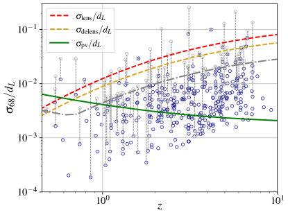
Figure 3: Scatter plot of the luminosity distance uncertainty at 1$\sigma$ from LISA parameter estimation as a function of redshift. Blue points correspond to all MBHBs simulated for the Q3d model and to the luminosity distance uncertainties adopted in the analysis. Green line represents the errors from peculiar velocities as in Eq. 19. Red (yellow) dashed line corresponds to the lensing error as in Eq. 16 without (with) the delensing correction. The grey dotted-dashed line corresponds to the arbitrary cut-off we impose on the $1\sigma$ error on $d_{L}$: we rerun the systems (grey points) whose $d_{L}$ error was originally above this grey line without the parameters describing the sky position of the binary, i.e. assuming perfect localisation thanks to the EM counterpart. For points below the grey line, the error on $d_{L}$ is, in all cases, dominated by lensing or peculiar velocities.

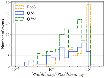
Figure 4: Ratio of the luminosity distance error without the sky position in the analysis over luminosity distance error from the full analysis. Both errors are at 90% level. Colors and line styles correspond to the three astrophysical models, as reported in the legend.

In Fig. 3, the grey points represent the luminosity distance uncertainty for the MBHBs simulated in the Q3d model as a function of redshift. As expected, lensing dominates the error budget at $z>2$ for the majority of sources while peculiar velocities are relevant only at $z<0.6$. However it is clear that there is a sub-population of events for which the uncertainty on the luminosity distance from LISA data analysis is larger than the lensing or peculiar velocities errors. Therefore, we decided to rerun the parameter estimation for the systems with $\sigma_{68,d_{L}}>0.5\,\rm\sigma_{\rm delens}$ or $0.5\sigma_{\rm pv}$ (the grey dotted-dashed line), assuming that the detection of the EM counterpart allow to localise precisely the galaxy hosting the merger. In this way, we can remove the two parameters describing the binary sky position from the inference of the GW signal and obtain better estimates on the luminosity distance (blue points).

In Fig. 4, we show the ratio of the luminosity distance uncertainties with and without the sky position for the subset of systems whose $d_{L}$ uncertainties was originally above the grey dotted-dashed line in Fig. 3. Overall, we find an improvement in the estimate of the luminosity distance up to one order of magnitude for the two massive models. However, in Pop3 the gain is slightly less, due to the intrinsic low mass of these systems that make the the parameter estimation more complicated. We have a single MBHB merger in the Q3nd model for which the ratio is larger than unity due to the stochastic behaviour of the MCMC chains.

To take into account the aforementioned sources of errors in luminosity distance for each MBHB event, we proceed in the following way:

1. We compute the $1\sigma$ dispersion of the luminosity distance posterior, $\sigma_{68,d_{L}}$, and shift all the $d_{L}$ samples by a random value extracted from $\mathcal{N}(0,\sigma_{68,d_{L}})$ where $\mathcal{N}$ is a Gaussian distribution;

2. To take into account the lensing and peculiar velocities errors, we scatter all the $d_{L}$ samples $x_{i}$ as

   $$x_{i,\mbox{new}}=x_{i}+x_{\mathcal{N}(0,\sigma_{\rm delens})}+x_{\mathcal{N}(0,\sigma_{\rm pv})}$$ (20)

   where $x_{\mathcal{N}(0,\sigma_{\rm delens})}$ and $x_{\mathcal{N}(0,\sigma_{\rm pv})}$ are random numbers extracted from a Gaussian distribution with zero mean and the corresponding standard deviation;

3. Finally, we shift all the samples by a random value extracted from $\mathcal{N}(0,\sqrt{\sigma^{2}_{\rm delens}+\sigma^{2}_{\rm pv}})$.

Step (1) models the effect of LISA noise realisations while steps (2) and (3) represent the fact that lensing and peculiar velocities are expected to spread our luminosity distance posteriors and to shift them with respect to the true value. At the end of this procedure, for each event, we have a new $d_{L}$ posterior distribution that is wider than the original one and not centered on the $d_{L}$ value from the assumed cosmology.

Moving to the redshift, it can be obtained by the EM counterpart. We assume that such measurement provides an estimate of the true source redshift $z_{true}$ and its uncertainty $\sigma_{z}$. The value of $\sigma_{z}$ depends on the technique adopted to detect the EM emission and on the magnitude of the source. If the EM emission is detected with LSST, we can measure the redshift of the source photometrically with an error $\sigma_{z}=0.031(1+z)$ Laigle et al. (2019). For ELT, if the source is sufficiently bright, the redshift can be spectroscopically estimated with $\Delta z=10^{-3}$. Otherwise, we can measure the redshift photometrically with the Lyman-$\alpha$ ($\Delta z=0.2$) or the Balmer break ($\Delta z=0.5$) as summarised in Tab. I of M22 (c.f. see also the discussion at the end of Sec. IVD). We also stress that while the spectroscopic error depends only on the spectral resolution of the instruments, the redshift uncertainties for the photometric measurements are more uncertain and it has to be considered as conservative. For ELT, these errors correspond to the 90% confidence interval. Therefore we can simply assume that, if the system is detected with ELT, $\sigma_{z}\simeq\Delta z/2$ where $\Delta z$ might be $10^{-3},\,0.2,\,0.5$.

Similarly to $d_{L}$, we also scatter our observations in redshift: for each EMcp, we extract a new redshift to perform the cosmological inference $z_{\rm em}$ as

$$z_{\rm em}=z_{\rm true}+\mathcal{N}_{\rm trunc}(0,\sigma_{z})$$ (21)

where $\mathcal{N}_{\rm trunc}$ is the truncated normal distribution, to avoid the extraction of negative redshift values at small redshift.

V Likelihood construction

In this section we describe the Bayesian formalism adopted in this study. Suppose we observe $N$ gravitational events $x_{\rm gw}=\{x_{\rm gw,1},\dots,x_{\rm gw,N}\}$ together with their corresponding EM counterparts $x_{\rm em}=\{x_{\rm em,1},\dots,x_{\rm em,N}\}$. The posterior distribution on the set of cosmological parameters $\theta_{c}$ based on some cosmological model $\mathcal{H}$ and on the total set of observations $\{x_{\rm gw},x_{\rm em}\}$ can be expressed as Del Pozzo (2012); Laghi et al. (2021)

$$p(\theta_{c}|x_{\rm gw}x_{\rm em}\theta_{m}\mathcal{H}\mathcal{I})=\frac{p(x_{\rm gw}x_{\rm em}|\theta_{c}\theta_{m}\mathcal{H}\mathcal{I})}{p(x_{\rm gw}x_{\rm em}|\theta_{m}\mathcal{H}\mathcal{I})}\pi(\theta_{c}|\mathcal{H}\mathcal{I})\,,$$ (22)

where $\theta_{m}$ collect the parameters describing the astrophysical populations and $\mathcal{I}$ collects all the necessary background information The quasi-likelihood $p(x_{\rm gw}x_{\rm em}|\theta_{c}\theta_{m}\mathcal{H}\mathcal{I})$ can be rewritten as a function of the GW signal and EM counterpart parameters. We define $\hat{\theta}_{\rm bin}$ as the set of GW signal parameters minus the luminosity distance $d_{L}$ and $\hat{\theta}_{\rm env}$ as the set of parameters describing the surrounding environment where the EM counterpart is produced minus the redshift $z$. In our case $\hat{\theta}_{\rm bin}$ corresponds to the two rest-frame BH masses, sky position, inclination, polarization, final phase and time to coalescence and the two spin magnitudes. The set of parameters $\hat{\theta}_{\rm env}$ corresponds to the parameters necessary to produce the EM counterparts as described in M22.

The quasi-likelihood $p(x_{\rm gw}x_{\rm em}|\theta_{c}\theta_{m}\mathcal{H}\mathcal{I})$ can be expanded as

$$p(x_{\rm gw}x_{\rm em}|\theta_{c}\theta_{m}\mathcal{H}\mathcal{I})=\frac{p^{\prime}(x_{\rm gw}x_{\rm em}|\theta_{c}\theta_{m}\mathcal{H}\mathcal{I})}{\alpha(\theta_{c}\theta_{m})}$$ (23)

$$\begin{split}p^{\prime}(x_{\rm gw}x_{\rm em}|&\theta_{c}\theta_{m}\mathcal{H}\mathcal{I})=\int d\hat{\theta}_{\rm bin}d\hat{\theta}_{\rm env}dd_{L}dz\\ &\times p(x_{\rm gw}x_{\rm em}|\hat{\theta}_{\rm bin}\hat{\theta}_{\rm env}d_{L}z\,\theta_{c}\theta_{m}\mathcal{H}\mathcal{I})\\ &\times p(\hat{\theta}_{\rm bin}\hat{\theta}_{\rm env}d_{L}z|\theta_{c}\theta_{m}\mathcal{H}\mathcal{I}).\end{split}$$ (24)

Let’s start working out the expression in the integral in Eq. 24. The second term in Eq. (24) defines how the parameters of the GW and EM events depend on the astrophysical population for a given cosmology. It can be split in the following way

$$p(\hat{\theta}_{\rm bin}\hat{\theta}_{\rm env}d_{L}z|\theta_{c}\theta_{m}\mathcal{H}\mathcal{I})=$$ (25)

$$p(\hat{\theta}_{\rm bin}\hat{\theta}_{\rm env}z|\theta_{c}\theta_{m}\mathcal{H}\mathcal{I})p(d_{L}|z\theta_{c}\mathcal{H}\mathcal{I})$$ (26)

where the first term determines how the parameters of the events depend on the population, whereas the second term $p(d_{L}|z\theta_{c}\mathcal{H}\mathcal{I})$ defines how luminosity distance and redshift are related. In the analysis we assume that $p(\hat{\theta}_{\rm bin}\hat{\theta}_{\rm env}z|\theta_{c}\theta_{m}\mathcal{H}\mathcal{I})$ can be treated as a constant in our inference. We do not fit the population parameters $\theta_{m}$ and we expect that $\hat{\theta}_{\rm bin}\hat{\theta}_{\rm env}$ to be mostly affected by astrophysical processes, rather than $\theta_{c}$ or the cosmological and background prior $\mathcal{H}\mathcal{I}$. Therefore, we assume that the impact of changing cosmology does not affect the distribution of events. Assessing this assumption would require rerunning the SAM model multiple times which is computationally prohibitive. For our purposes, constant quantities can be discharged so only the term $p(d_{L}|z\theta_{c}\mathcal{H}\mathcal{I})$ remains.

The first term in the integral of Eq. (24) defines how the GW and EM data {$x_{\rm gw},x_{\rm em}$} are related to the models that fit the data. It can be simplified assuming that the GW and EM measurements are independent. We also suppose that GW event depends only on the binary parameters, leading to

$$\begin{split}p(x_{\rm gw}x_{\rm em}|\hat{\theta}_{\rm bin}\hat{\theta}_{\rm env}d_{L}z\,\theta_{c}\theta_{m}\mathcal{H}\mathcal{I})&=p(x_{\rm gw}|\hat{\theta}_{\rm bin}d_{L}\,\theta_{c}\mathcal{H}\mathcal{I})\\ &\times p(x_{\rm em}|\hat{\theta}_{\rm env}\theta_{c}z\mathcal{H}\mathcal{I}).\end{split}$$ (27)

We assume that the EM observation depends only on the redshift of the source, and we can write the EM counterpart likelihood as:

$$\begin{split}\int d\hat{\theta}_{\rm env}p(x_{\rm em}|\hat{\theta}_{\rm env}\theta_{c}z\mathcal{H}\mathcal{I})=p(z_{em}|z).\end{split}$$ (28)

Moreover, the luminosity distance can be expressed as a function of $z$ and the cosmological parameters $\theta_{c}$ so we can rewrite the integral in Eq. 24 as

$$\begin{split}p^{\prime}(x_{\rm gw}x_{\rm em}|&\theta_{c}\theta_{m}\mathcal{H}\mathcal{I})=\int d\hat{\theta}_{\rm bin}dd_{L}dz\,\\ &\times p(x_{\rm gw}|\hat{\theta}_{\rm bin}d_{L}\,\theta_{c}\mathcal{H}\mathcal{I})\,p(z_{em}|z)\\ &\times\delta(d_{L}-d_{L}^{c}(z,\theta_{c}))\end{split}$$ (29)

where $d_{L}^{c}(z,\theta_{c})$ is the luminosity distance according to a specific cosmological model as the ones specified in Sec. III and the $\delta(\dots)$ comes from the $p(d_{L}|z\theta_{c}\mathcal{H}\mathcal{I})$ term. The quantity $p(x_{\rm gw}|\hat{\theta}_{\rm bin}d_{L}\,\theta_{c}\mathcal{H}\mathcal{I})$ can be expressed as the ratio between the posterior distribution of the binary parameters and the prior, i.e.

$$p(x_{\rm gw}|\hat{\theta}_{\rm bin}d_{L}\,\theta_{c}\mathcal{H}\mathcal{I})=\frac{p(\hat{\theta}_{\rm bin}d_{L}|x_{\rm gw})}{p(\hat{\theta}_{\rm bin}d_{L})}.$$ (30)

Since we assumed uniform prior, Eq. 29 becomes

$$\begin{split}p^{\prime}(x_{\rm gw}&x_{\rm em}|\theta_{c}\theta_{m}\mathcal{H}\mathcal{I})=\int dd_{L}dz\,\\ &\times\,p(d_{L}|x_{\rm gw})\,p(z_{\rm em}|z)\,\delta(d_{L}-d_{L}^{c}(z,\theta_{c}))\end{split}$$ (31)

where we marginalized over $\hat{\theta}_{\rm bin}$ to obtain $p(d_{L}|x_{\rm gw})$.

The property of the delta function $\delta(f(z))=\delta(z-z_{0})|\partial_{z}f(z_{0})|^{-1}$, where $f(z_{0})=0$ allows to rewrite the above equation as follows

$$p^{\prime}(x_{\rm gw} x_{\rm em}|\theta_{c}\theta_{m}\mathcal{H}\mathcal{I})=\int dd_{L}dz\,p(d_{L}|x_{\rm gw})\,$$ (32)

$$\times\,p(z_{\rm em}|z)\delta(z-z^{c}(d_{L},\theta_{c}))\left|\frac{dd_{L}(z,\theta_{c})}{dz}\right|^{-1}\,,$$ (33)

where we denote $z^{c}(d_{L},\theta_{c})$ as the redshift for a given luminosity distance and cosmological parameters, i.e. the inverse of $d_{L}^{c}(z,\theta_{c})$. We can now solve the integral in redshift and obtain

$$p^{\prime}(x_{\rm gw} x_{\rm em}|\theta_{c}\theta_{m}\mathcal{H}\mathcal{I})=\int dd_{L}\,p(d_{L}|x_{\rm gw})\,$$ (34)

$$\times\,p(z_{\rm em}|z^{c}(d_{L},\theta_{c}))\left|\frac{dd_{L}(z^{c}(d_{L},\theta_{c}),\theta_{c})}{dz}\right|^{-1}\,.$$ (35)

From the LISA parameter estimation we have the posterior $p(d_{L}|x_{\rm gw})$ and the associated samples $d^{i}_{L}$. This allows to evaluate the integral in a Monte Carlo way:

$$p^{\prime}(x_{\rm gw} x_{\rm em}|\theta_{c}\theta_{m}\mathcal{H}\mathcal{I})=$$ (36)

$$\sum_{d_{L}^{i}\in p(d_{L}|x_{\rm gw})}p(z_{\rm em}|z^{c}(d^{i}_{L},\theta_{c}))\left|\frac{dd_{L}(z^{c}(d^{i}_{L},\theta_{c}),\theta_{c})}{dz}\right|^{-1}\,.$$ (37)

For the likelihood of the EM counterpart we adopted a Gaussian form as

$$p(z_{\rm em}|z)=\frac{1}{\sqrt{2\pi\sigma^{2}_{z}}}\exp{\Big{[}-\frac{1}{2}\frac{(z_{\rm em}-z)^{2}}{\sigma^{2}_{z}}\Big{]}}.$$ (38)

The quantity $\alpha(\theta_{c}\theta_{m})$ in Eq. 23 is the selection function and it takes into account that not all the GW events or all the EM counterparts are observed Mandel et al. (2019) The fact that we observe only a sub-sample of the entire population might lead to biased estimates if not properly accounted for. On a practical level, selection effects can be understood thinking that, for example, some combinations of $h$ and $\Omega_{m}$ might move sources outside/inside the GW (or EM) horizon changing the luminosity distance of the source. The computation of the selection function requires the integration of the integral in Eq. 24 over all the possible combinations of $\{x_{\rm gw},x_{\rm em}\}$ above the respective detection thresholds. Before delving into the calculation of this quantity, we checked how the number of EM counterparts changes for different values of $(h,\Omega_{m})$. We picked the median realisation for the Q3d model and the pair of samples $(h,\Omega_{m})$ that give the smallest and largest luminosity distance. For these two values of $d_{L}$ we recomputed the EM counterpart for each MBHB in our catalogs and we rescaled the sky localization as in Klein et al. (2016) in order to quantify the number of EMcps that could enter or exit the analysis, varying the cosmological parameters. For Q3d we find a difference of $\sim 0.35$ EMcps in 4 yr of observation. Since the variation is negligible, we simply assume that $\alpha(\theta_{c}\theta_{m})\sim\rm const.$, and neglect its contribution in the analysis. This assumption is also motivated by the actual results of cosmological inference because we do not observe any strong bias coming from selection effects.

VI Inference analysis

Table 2: Inferred parameters and the corresponding priors for the ‘Local Universe’ models. In agreement with Belgacem et al. (2019), in the last model, we adopt normal priors as $\mathcal{N}[\mu,\sigma]$ (for $\omega_{0},\,\Xi_{0}$ we consider truncated normal distributions). In the last case, the prior on $h$ and $\Omega_{m}$ are based on CMB+BAO+SNe data.

Model	Parameter	Prior
$(h,\Omega_{m})$	$h$	$\mathcal{U}[0.2,1]$
	$\Omega_{m}$	$\mathcal{U}[0,1]$
$(h,\Omega_{m},\omega_{0},\omega_{a})$	$h$	$\mathcal{U}[0.2,1]$
	$\Omega_{m}$	$\mathcal{U}[0,1]$
	$\omega_{0}$	$\mathcal{U}[-3,-0.3]$
	$\omega_{a}$	$\mathcal{U}[-2,2]$
$(h,\Omega_{m},\omega_{0},\Xi_{0})$	$h$	$\mathcal{N}[0.6774,0.012]$
	$\Omega_{m}$	$\mathcal{N}[0.3075,0.0124]$
	$\omega_{0}$	truncated $\mathcal{N}[-1,1]$ in $[-3,-0.3]$
	$\Xi_{0}$	truncated $\mathcal{N}[1,0.5]$ in $[0,+\infty]$

Table 3: Inferred parameters and the corresponding priors for the ‘High-redshift Universe’ models. First three columns as in Tab. 2. Fourth and fifth columns represent the pivot redshift (if applicable) and the corresponding redshift range. In the last column we report the number of EMcps in 10 yr in the redshift range. For most of the parameters we choose uniform priors but see Sec. VI for more details. For the priors on the splines check specifically Sec. VI.3.

Model	Parameter	Prior	$z_{p}$	$[z_{\rm min},z_{\max}]$	EMcps in 10 yr
$(h,\Omega_{m},\beta)$	$h$	$\mathcal{U}[0.2,1]$	-	[$0,+\infty$]	16.0
	$\Omega_{m}$	$\mathcal{U}[0,1]$			37.0
	$\beta$	$\mathcal{U}[-3,3]$			51.7
Matter-only approx.	$d_{C}(z_{p})$/Gpc $h(z_{p})$	$\mathcal{U}[1,9]$ $\mathcal{U}[0.2,5]$	2	$[1,+\infty]$	13.2
					31.2
					43.2
			3	$[1.5,+\infty]$	11.0
					27.2
					36.2
Redshift bins	$d_{C}(z_{p})$/Gpc $h(z_{p})$	$\mathcal{U}[0.1,50]$ $\mathcal{U}[0.1,50]$	1	$[0.8,1.3]$	1.9
					2.8
					5.1
			1.5	$[1.2,2.0]$	3.2
					6.0
					9.1
			2	$[1.7,2.8]$	3.9
					8.9
					11.2
			2.5	$[2.0,3.5]$	4.9
					11.3
					15.3
			3	$[2.0,4.0]$	6.1
					14.7
					20.7
			3.5	$[2.6,5.0]$	5.7
					15.2
					20.3
			4	$[3.0,5.0]$	4.1
					13.1
					17.0
			5	$[3.5,6.0]$	3.9
					12.5
					16.1
Splines interp.	$d_{L}(z=0.2)$	$d_{L}^{\Lambda{\rm CDM}}$	-	[$0,7$]	16.0 35.8 51.5
	$d_{L}(z=0.7)$
	$d_{L}(z=2)$
	$d_{L}(z=4)$
	$d_{L}(z=6)$

Following the procedure described in Sec. IV, we generate 100 realisations of 4 and 10 yr of LISA observations for the three astrophysical models. We run the MCMC for 2500 iterations with $n\times 16$ walkers where $n$ corresponds to the number of parameters in the model.

In Tab. 2 we report the prior range for the parameters over which we performed the inference in the ‘Local Universe’ models. In the first two cases we assume uniform priors while for the $(h,\Omega_{m},\omega_{0},\Xi_{0})$ model, we follow the same approach of Belgacem et al. (2019): since the proposed modification can be measured only with GWs, we assume CMB+BAO+SNe priors for $h$ and $\Omega_{m}$.

Moving to the ‘High-redshift Universe’ scenarios, we assume uniform priors for the $(h,\Omega_{m},\beta)$ model. However additional considerations are necessary for the other approaches.

VI.1 Matter-only approximation

Since in the matter-only model we assume that the Universe is matter-dominated, we have to choose values of $z_{p}$ sufficiently large. In our case we consider two values: $z_{p}=2$ and $z_{p}=3$. In the former case, the matter-only approximation is accurate at $\sim 2-1\%$ in the redshift range $1<z<7$, while in the latter we have an accuracy of $\sim 4\%$ already at $z=1$. As a consequence, in order to avoid significant biases in the reconstructed parameters, we chose to remove the EMcps at low redshift. In particular, in the case $z_{p}=2$, we remove all the EMcps at $z<1$ while for $z_{p}=3$ we remove all systems at $z<1.5$. We do not apply any cut at high redshift where deviations are below $\sim 1\%$ at $z=10$.

VI.2 Redshift bins approach

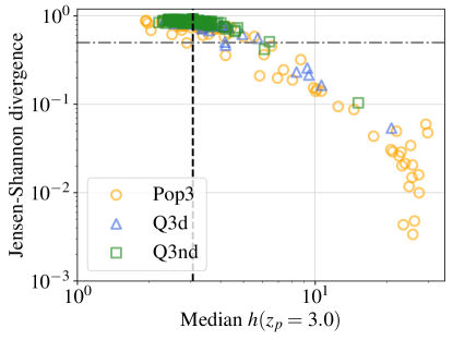
Figure 5: Example of JS divergence computed between the posterior distribution of $h(z_{p}=3)$ and an uniform prior between $[0.1,50]$ versus the inferred median value of $h(z_{p}=3)$. Each point corresponds to a single realisation for each astrophysical model, according to legend. The horizontal grey dotted-dashed line corresponds to the arbitrary cut-off of 0.5 on the value of the JS divergence (more details in the text). The blacked dashed line represents the true value of $h(z_{p}=3)\sim 3.06$, according to $\Lambda$CDM. Uninformative realisations show inferred median values at $\sim 25$, corresponding to the midpoint of the prior range, and JS divergence closer to 0, i.e. the posterior is similar to the prior.

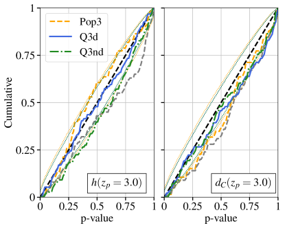
Figure 6: Cumulative distribution of events with p-value smaller or equal to the abscissa. Colors and line styles according to legend. The dotted lines represent the 90% uncertainty region expected from the finite number of realisations. The dashed black line represents the expected value. Grey dashed line: same as the orange one for Pop3 but including all the realisations. It is clear that selecting only the informative realisations provide results consistent with the expected values.

In the redshift bins approach we approximate the comoving distance as Eq. 14 in a redshift interval. Therefore we consider only the EMcps that fall in that particular bin and discharge all the others . One can easily see that there are two competing effects: on one hand, one would like to increase the size of the redshift bin as much as possible in order to include more EMcps; on the other hand, extending the redshift range leads to an inaccurate representation of the $d_{C}-z$ relation (the relation is not anymore a straight line) which introduce significant biases in the recovered $(h(z_{p}),d_{C}(z_{p}))$. The redshift bins approach might also leads to biased results for the comoving distance by construction: if we have EMcps only close to the bin edges, the inference recovers a comoving distance that it slightly smaller than the expected value at the pivot redshift, while the slope is still the same. Therefore the lower and upper limit of the redshift bin play an important role in the inference and we choose them in order to have the maximum number of EMcps in a redshift bin without compromising the recovered parameters or the accuracy ($\lesssim 3\%$ in most cases) between the linear approximation and $\Lambda$CDM.

Depending on the astrophysical models and on the redshift bin we might not have many EMcps ( at low or high redshift) or the EMcps in the bins might have large $d_{L}$ and $z$ uncertainties (at high redshift). In these cases, we have to be extra cautious because if the data are not sufficiently informative, the priors play a pivotal role.

For both $h(z_{p})$ and $d_{C}(z_{p})$ we impose an uniform prior between $[0.1,50]$ (in the corresponding units). However, in standard $\Lambda$CDM, we expect that $h(z=0)=0.6774$ and $h(z=7)\sim 8.5$. Considering these values, a prior extending up to 50 might seem too broad and not realistic of our current and future ‘degree of belief’ on $h(z)$. Here we justify our choice.

Originally we had chosen smaller priors for $h(z_{p})$ and $d_{C}(z_{p})$, symmetric and centered on the true values assuming $\Lambda$CDM. However, after a deeper inspection of the results, we noticed that some realisations were not informative, i.e. the posteriors on $h(z_{p})$ and $d_{C}(z_{p})$ were identical to the priors. As expected, this happened if the data were not sufficiently informative, i.e. small number of EMcps in a given bin or $d_{L}$ and $z$ uncertainties too large. Without accounting for these uninformative realisations, our forecasts would have been prior dominated.

To distinguish between informative and uninformative realisations, we apply the Jensen-Shannon (JS) divergence Lin (1991) between the posterior and the prior distributions for $h(z_{p})$ and $d_{C}(z_{p})$. Our argument is that, if the realisation is informative, the posterior distribution will be significantly different from the prior and the JS divergence will be close to 1. If the realisation is uninformative the posterior will be instead similar to the prior and the JS will be closer to 0.

In Fig. 5 we show an example of the JS divergence computed between the posterior in $h(z_{p})$ and a flat uniform prior in $[0.1,50]$. On the x-axis we report the inferred median value of $h(z_{p}=3)$. Especially for Pop3, it is clear that there is a sub-population of realisations with median value $h(z_{p}=3)\sim 25$ (the midpoint of the bin) and low JS divergence, indicating that those realisations would not provide any constraint on $h(z_{p}=3)$. As expected Pop3 show the largest number of uninformative realisations due to the smaller average number of EMcps and larger errors on luminosity distance and redshift.

In order to get rid of the uninformative cases, we select as informative realisations only the ones with JS divergence $>0.5$ . This value is somewhat arbitrary but we provide more details on this choice in Appendix C. We decide to apply this criteria only on the posterior distribution for $h(z_{p})$ because it’s the parameter we are mostly interested in in this approach.

Moreover, in order to further support the choice of this value, we present a probability-probability (PP) plot of the p-value following the approach in The LIGO Scientific Collaboration et al. (2021b) and considering only the informative realisations. For each informative realisation, we compute the quantile in which is contained the true value and we assume $n=$p-value$\times\rm N$ and $\rm N=\rm N_{info-real}$ where $\rm N_{info-real}$ corresponds to the number of informative realisations. We show an example of the PP plot for $z_{p}=3$ in Fig. 6. For $h(z_{p})$, the pp-plots follow the diagonal line and they are compatible with the corresponding errors. The results for $d_{C}(z_{p})$ are a bit worse but still compatible with the overall errors. This is due to the nature of the bin approach which tends to produce slightly biased results for the comoving distance. It’s also clear that, if we include all the realisations ($\rm N=100$), there is a significant deviation in the cumulative distribution of the p-value from the expected one, as showed by the grey line.

We note that the JS divergence and the PP plot tell us two different information: the former quantify the difference between the posterior and the prior distribution without telling us where the posterior peaks; the latter tell us the fraction of realisations that contain the true value in a given percentile interval.

In all the results for the redshift bins approach, we applied the JS divergence and the PP-plot to assess the number of informative realisations. We extended this analysis also for the other cosmological models but we found no particular issues with them. We note indeed that these tests were necessary for the particular nature of the redshift bins approach: most of the other models adopt a functional form for the $d_{L}-z$ relation that is more complicated than a simple straight line and cover a wider range of redshifts. Therefore, even with a smaller number of EMcps, these models can provide reasonable constraints because we are adding an ‘a priori’ additional information on our Universe model. The only exception is represented by the splines interpolation model. However, in this case, we have typically more EMcps than in the redshift bins case.

Finally, since the bin approach is the most sensitive to the number of EMcps, we perform this analysis assuming only the scenario of 10 years of time mission. If LISA will provide data for only 4 yr, this analysis could not be performed.

VI.3 Splines interpolation

For the splines interpolation model, we approximate the luminosity distance with cubic polynomials. We fix the knots at $z=[0.2,0.7,2,4,6]$ with the additional information that the luminosity distance $d_{L}(z=0)=0$. In order to avoid issues at high redshift, we remove all the systems at $z>7$. The result of the inference is a 5-dimensional posterior distribution of the $d_{L}$ values at the aforementioned knots. The $d_{L}$ posteriors can then be easily converted into $d_{C}$ posteriors at the knot redshifts and we can evaluate the slope of the splines to obtain information on $H(z)$ at any redshift. Contrary to the redshift bins model, splines allow us to use the entire population of EMcps. To construct the prior on the luminosity distance at a given knot, we take samples from the uniform priors in $(h,\Omega_{m})$ and convert them in $d_{L}$ assuming $\Lambda$CDM, i.e. according to Eq. 5. The resulting $d_{L}$ distribution is assumed as the prior and we repeat this process at each of the knots. We note that we use $\Lambda$CDM only to fix the priors for the luminosity distance: the splines approach is model-independent, and we have tested that the choice of priors does not impact our results.

VII Results

In this section we present the results of our inference analyses applied to the cosmological models mentioned in Sec. III. In what follows relative uncertainties on the inferred parameters are reported for the Q3d (Pop3) {Q3nd} model following this bracket convention.

VII.1 Local Universe results

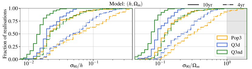
Figure 7: Cumulative distributions of the relative uncertainties for $h$ (left panel) and $\Omega_{m}$ (right panel) in the $(h,\Omega_{m})$ model, namely $\Lambda$CDM. Solid (dashed) lines correspond to 10 (4) yr of observations. Colors represent different astrophysical models as described in the legend and the grey area represents uncertainties larger than $100\%$. We expect relative errors of $\lesssim 5\%$ for $h$ in 4 yr and $\lesssim 2\%$ in 10 yr. For $\Omega_{m}$, we forecast relative errors $\lesssim 10\%$ only in 10 yr.

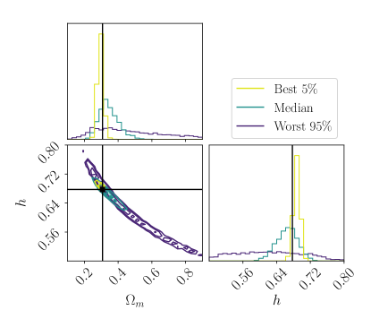
Figure 8: Corner plot for $(h,\Omega_{m})$ for the median, the 5th and 95th percentile realisations of Q3d (more details in the text) for the $(h,\Omega_{m})$ model in 4 yr. Colors according to legend.

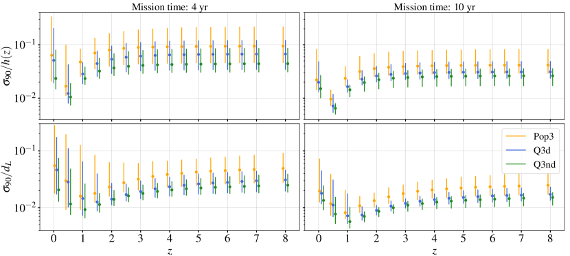
Figure 9: Relative errors at 90% for $h(z)$ (upper panels) and $d_{L}(z)$ (lower panels) as a function of redshift from the $(h,\Omega_{m})$ model, i.e. assuming $\Lambda$CDM. Error bars also correspond to $90\%$. Colors correspond to different astrophysical models, according to the legend. Uncertainties are obtained from the $(h,\Omega_{m})$ samples, assuming Eq. 5 . To be compared with Fig. 2 of Bull et al. (2021) but note that they report the uncertainties at $1\sigma$ so our values must be divided by a factor $\sim 1.6$ for proper comparison. To avoid null values in the lower panels, the first point for $d_{L}$ is at $z=0.1$.

In Fig. 7 we report the relative errors at 90% confidence level for $h$ and $\Omega_{m}$ as in the $(h,\Omega_{m})$ model (aka $\Lambda$CDM,) for 4 yr and 10 yr of LISA mission. For the relative uncertainty on $h$, we predict a median uncertainty of $5.1\%$ ($6.3\%$) {$2.3\%$} in 4 years. These figures improve to $2.0\%$ ($2.2\%$) {$1.5\%$} in 10 years.

Overall Q3nd provides the best estimates because it has on average $\sim 3$ times more EMcps than Pop3. However moving from 4yr to 10yr of observations, the uncertainties for the Pop3 model reduce by a factor $\sim 3$ while in Q3nd the reduction is only $\sim 1.5$. This is due to the fact that the estimates on the cosmological parameters improves as $\sim N_{EMcps}^{-1/2}$ so we have larger improvements when the number of events is small. Our estimates are affected by large uncertainties: for the Q3d model and in 4 yr, for example, the relative uncertainty vary from few percent up to $\sim 20\%$. As we move to 10 yr, the uncertainties variability decreases because we have more EMcps and we are less sensitive to single events in each realisation.

For $\Omega_{m}$, we expect relative uncertainties of $23\%$ ($32\%$) {$13\%$}, in 4 yr and of $10\%$ ($12\%$) {$8\%$} in 10 yr. We note that $h$ is typically determined better than $\Omega_{m}$. Indeed the former corresponds to the first derivative of $d_{L}(z)$ at $z=0$ and $d_{L}(z=0)=0$ is fixed. This means that a single precise measurement at high $z$ can constrain $h$ to a tight value (similarly to the CMB). To constrain $\Omega_{m}$ we need to probe the curvature (e.g. second derivatives) of $d_{L}(z)$ meaning that we need multiple precise measurements at high-redshift, i.e. where the curvature of $d_{L}(z)$ is more pronounced, to get a good precision on $\Omega_{m}$.

In Fig. 8 we show the correlation between $(h,\Omega_{m})$ for three representative realisations of Q3d for the case of 4 yr. We ranked all the realisations according to the area covered by the samples. This quantity keeps track of the correlation between the two parameters and it is more representative than the separate error in each of them. Following this procedure, we obtain the areas for all the 100 realisations in Q3d. Here we plot the realisations with the area closest to the median, the 5th and the 95th percentiles. The parameters $(h,\Omega_{m})$ are negatively correlated because small values of $h$ require large value for $\Omega_{m}$ to compensate in the $d_{L}-z$ relation. We highlight this feature as other cosmological probes have different orientations for the correlation. For example, EMRIs are expected to have more positive correlation between $h$ and $\Omega_{m}$ Laghi et al. (2021) and combining different types of sources we would be able to further break degeneracies between cosmological parameters Tamanini (2017); Laghi et al. ; Betoule et al. (2014).

We also use the samples on $(h,\Omega_{m})$ to get the errors on $h(z)$ or $d_{L}(z)$ at higher redshifts. Following Eq. 5 and Eq. 6, we can convert each pair of $(h,\Omega_{m})$ samples in a sample for $h(z)$ or for the luminosity distance at any redshift. We note that the forecasts obtained in this case are based on the assumption of $\Lambda$CDM. In Fig. 9 we report the relative errors on $h(z)$ and $d_{L}(z)$ as a function of redshift. The best constraints on $h(z)$ are achieved at $z\sim 0.5$, because at low redshift we expect better constraints on $h_{0}$ than on $\Omega_{m}$ and vice-versa at high redshift. Moreover, we also find that $z\sim 0.5$ is where the correlation between $h(z)$ and $\Omega_{m}$ is zero (more details in Appendix D). Starting from 4 yr of time mission, at $z\sim 0.5$ we expect a relative uncertainty on $h(z)$ of $1.2\%$ ($1.7\%$) {$1.0\%$}. Above $z\gtrsim 2$, the relative errors flatten around $7\%$ ($9\%$) {$4\%$} while at $z=0$ we recover the previous results. If we will have 10 years of data, the uncertainties at $z\sim 0.5$ will improve to $0.7\%$ ($0.9\%$) {$0.6\%$} while at $z\gtrsim 2$ the relative uncertainties will be between $2\%$ and $5\%$ , depending on the MBHB population model.

For $d_{L}(z)$, we find the same trends of $h(z)$ but the best constraints are obtained at $z\sim 1$. In particular, in 4 yr at $z\sim 1$ we predict $d_{L}(z)$ relative errors of $1.4\%$ ($1.6\%$) {$0.9\%$}. While in 10 yr, we expect the errors to be between $0.5\%$ and $0.8\%$ at $z\sim 1$ and at $\sim 1-2\%$ for $z\gtrsim 4$.

The results from MBHBs can be compared to other cosmological probes. In particular, we can compare Fig. 9 with Fig. 2 of Bull et al. (2021): note that we are plotting the $90\%$ error while they are reporting the $1\sigma$ uncertainty so the values from Fig. 9 should be divided by a factor $\sim 1.6$ for a proper comparison. At low redshift, the results for $h(z)$ with MBHBs are slightly worse than what we might be able to do with other cosmological probes: in 4yr, at $z\sim 1$ the median relative error for Q3d is $\sim 4$ times larger than the forecasts for HIRAX and one order of magnitude larger than the ones expected from DESI. However MBHBs provide comparable results with an high-redshift version of HIRAX at $z>5$. Concerning the luminosity distance, at $z\sim 1$, the relative error from Q3d model is $<2$ larger than the forecasts from DESI but at the same level of HIRAX. As we move to higher redshifts our forecasts tend to flatten thanks to the high-redshift sources while the predictions from EM probes degrade quickly: for example MBHBs predict better constraints than a high-redshift version of HIRAX at $z\sim 4$ and than a stage 2 intensity mapping experiment at $z\sim 6$ .

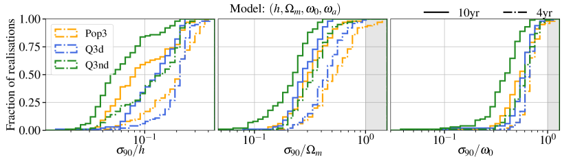
Figure 10: Same as Fig. 7 but with $h,\Omega_{m}$ and $\omega_{0}$ from the $(h,\Omega_{m},\omega_{0},\omega_{a})$ model. $\omega_{a}$ is unconstrained and not reported. The addition of two parameters worsen the estimates on $(h,\Omega_{m})$.

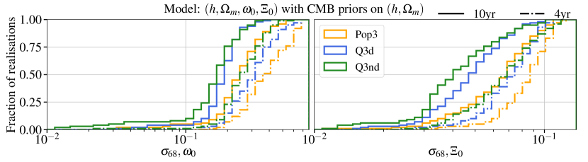
Figure 11: Absolute uncertainties at $1\sigma$ for $\omega_{0}$ and $\Xi_{0}$ for the $(h,\Omega_{m},\omega_{0},\Xi_{0})$ model. Note that we report the absolute $1\sigma$ uncertainties for comparison with Tab.2 in Belgacem et al. (2019). The uncertainties on $h$ and $\Omega_{m}$ are not reported because they coincide with the CMB priors. We can constrain $\Xi_{0}$ to $<10\%$ using only standard sirens.

For the $(h,\Omega_{m},\omega_{0},\omega_{a})$ model, we report the uncertainties on $h$, $\Omega_{m}$ and $\omega_{0}$ in Fig. 10. As expected, the presence of two additional parameters worsen the estimates on $h$ and $\Omega_{m}$. In 10 yr, $h$ is constrained to $\sim 10\%$ accuracy and $\Omega_{m}$ at $\sim 20-30\%$. We also find that $\omega_{0}$ is poorly constrained with uncertainties $>30\%$ in all cases while $\omega_{a}$ is unconstrained. As showed by previous work Tamanini et al. (2016); Belgacem et al. (2019), we conclude saying that in this scenario LISA could hardly provide information.

In Fig. 11 we report the uncertainties on $\Xi_{0}$ and $\omega_{0}$ for the $(h,\Omega_{m},\omega_{0},\Xi_{0})$ model. For this scenario we adopt the same CMB priors of Belgacem et al. (2019) in order to assess LISA ability to constrain $\Xi_{0}$ only with standard sirens and we report the $1\sigma$ uncertainty. In comparison to Belgacem et al. (2019), we obtain uncertainties on $\Xi_{0}$ approximately 2-3 times larger. This is due to the fact that, in Belgacem et al. (2019), the authors also included information from CMB, BAO, and SNe, leading to a better estimate of $\omega_{0}$ and, consequently, of $\Xi_{0}$ (this can be appreciated from their Fig. 17 and Fig. 18). In 4 yr, the median relative errors on $\Xi_{0}$ are $7.6\%$ ($8.9\%$) {$7.0\%$}. Assuming 10 years of observation, the estimates improve to $4.9\%$ ($7.1\%$) {$4.1\%$}, respectively. Due to the choice of priors on $h$ and $\Omega_{m}$, the uncertainties on these parameters are comparable with the prior, i.e. the priors are too strong respect to the data, so we choose not to report them.

We can also compare our results with the forecasts for EMRIs Liu et al. (2023), although, in this case, the comparison is not straightforward due to the different analysis setups. In their fiducial model and assuming only $\Xi_{0}$ as free parameter, the authors report an error of $8.5\%$ at 90% C.I. This value is slightly better than our results in 4 yr. However, when more parameters are left free to vary, the reported errors on $\Xi_{0}$ in Liu et al. (2023) are larger than ours. Taking into account the uncertainties from the different priors adopted, we expect MBHBs and EMRIs to provide similar constraints on $\Xi_{0}$.

VII.2 High-redshift Universe results

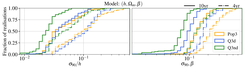
Figure 12: Same as Fig. 7 but for $h$ and $\beta$ for the $(h,\Omega_{m},\beta)$ model. The parameter $\beta$ models possible deviation for the matter equation of state, i.e. $\omega_{m}=\beta$ and it should be constrained with a relative accuracy of $<20\%$ with 4 yr of observations and $\lesssim 10\%$ in 10 yr.

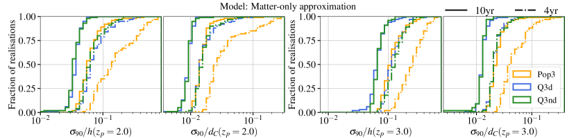
Figure 13: Same as Fig. 7 but for $h(z_{p})$ and $d_{C}(z_{p})$ from the matter-only approximation. Left panels: $z_{p}=2$. Right panels: $z_{p}=3$. In 10yr of observation, we expect constraints on $h(z_{p}=2)$ at $3-5\%$ and on $h(z_{p}=3)$ at $\lesssim 10\%$.

In Fig. 12 we report the results of the analysis for the $(h,\Omega_{m},\beta)$ model, i.e. assuming $\omega_{m}=\beta$ as the matter equation of state. As expected, the addition of $\beta$ worsen the constraining power on $h$. In 4 yr, $h$ is constrained at $11\%$ ($10\%$) {$4.9\%$}, while in 10 yr the estimates improve to $3.8\%$ ($3.4\%$) {$2.5\%$}.

Concerning the matter part, $\Omega_{m}$ and $\beta$ are degenerate: if $\beta$ decreases, $\Omega_{m}$ increases to compensate. We find that in 4 yr $\Omega_{m}$ is unconstrained and, for this reason, we decided to not plot it. In 10 yr, $\Omega_{m}$ can be constrained with large uncertainties of $\sim 30-40\%$. For $\beta$, we expect constraints of $18\%$ ($23\%$) {$14\%$} and $10\%$ ($14\%$) {$8.0\%$} in 4 yr and 10 yr, respectively.

The fact that $\beta$ is constrained while $\Omega_{m}$ is not can be understood looking at how they appear in Eq. 12. While $\Omega_{m}$ acts a multiplicative factor, $\beta$ is an exponential. Therefore a small variation in $\beta$ can lead to a large difference in the expected luminosity distance. Or, in other words, if $\beta$ varies, $\Omega_{m}$ has to vary even more in order to compensate and reproduce the expected $d_{L}-z$ relation.

Moving to the matter-only approximation, in Fig. 13 we report the relative uncertainties at $90\%$ on $h(z_{p})$ and $d_{C}(z_{p})$ for $z_{p}=2$ and $z_{p}=3$. Starting from $h(z_{p})$, we find overall better results at $z_{p}=2$ than $z_{p}=3$. For example, in 10 yr we predict median errors of $3.8\%$ ($6.0\%$) {$3.6\%$} at $z_{p}=2$ and $6.8\%$ ($11\%$) {$6.8\%$} at $z_{p}=3$. We recall that for the case at $z_{p}=2$ ($z_{p}=3$), we removed all the systems at $z<1$ ($z<1.5$). As a consequence, the case $z_{p}=2$ contains overall more standard sirens than the one at $z_{p}=3$, leading to better estimates.

Moving to the comoving distance $d_{C}(z_{p})$ and still in 10 yr, we expect relative uncertainties at $0.9\%$ ($1.5\%$) {$0.9\%$} at $z_{p}=2$ and $1.3\%$ ($2.3\%$) {$1.3\%$} at $z_{p}=3$. Similarly to the case for $h(z_{p})$, we obtain better estimates at $z_{p}=2$ than at $z_{p}=3$.

It is interesting to compare these results with the uncertainties reported in Fig. 9. The estimates on $h(z_{p}=2)$ in the matter-only approximation are marginally worse while at $z=3$ the difference increases to a factor of $\sim 2-3$. This is expected because in the matter-only approximation we removed the low-redshift sources so there are effectively less EMcps. The results for the distance uncertainties are more similar between the two approaches: we think that the explanation resides in the fact that the comoving distance appears in Eq. 13 as a simple normalizing factor for the whole expression, leading to better estimates even with less EMcps.

In Fig. 14 we report the uncertainties on $h(z_{p}$) and $d(z_{p})$ from the redshift bins approach, assuming 10 yr of observation. Following the discussion in Sec. VI.2, the cumulative distributions do not reach the value of 1 but the fraction of informative realisation in that particular redshift bin. For example at $z_{p}=1$, we have $49$ ($43$) {$77$} informative realisations out of 100 in total. It can be appreciated that the number of informative realisation is small at low redshift ($z_{p}=1$), then it start increasing, reaching the maximum at $z_{p}=3$ and then it decreases again at higher redshifts. The largest fraction of informative realisations at $z_{p}=2.5-3$ reflects the redshift distribution of merging MBHBs (c.f. solid green line in Fig.1 of M22). At $z<1.5$ we do not expect many events so the number of uninformative realisations increases. The same argument can be applied at high redshift $z>3.5$, where we also expect larger errors on the luminosity distance and redshift of the source.

A part from $z_{p}=1$ where the number of informative realisation is below $50\%$ even for Q3d, we have the best constraints on $h(z_{p})$ at $z_{p}=3$ with $75\%$ of the realisation predicting a relative error on $h(z_{p})$ smaller than $30\%$ for the massive models, while this fraction decreases to only $25\%$ for Pop3. Comparing these results with the uncertainties reported in Fig. 9, it is clear that the redshift bins approach is less performing. Even if the prospect of a model-independent test is appealing, the small number of EMcp in each bin makes it feasible only between $1.5<z<3.5$ if the Q3 models are the correct ones.

Motivated by the model-independent technique adopted with the redshift bins, we searched for another model-independent method that could allow us to use the entire set of EMcps. The results of this search is the splines interpolation model, whose results are reported in Fig. 15. Starting from $d_{L}$, we predict errors $<10\%$ between $0.7<z<4$ in 4 yr of observations. In the case of 10 yr of observation, we reach $1-2\%$ precision in between $0.7<z<3$ while at $z>4$ we have few percents precision uncertainties with wider error bars. If we compare our results with Fig.2 of Bull et al. (2021), we see that splines provide estimates that are competitive with future EM observations. The fact that we obtain better estimate at $z\sim 6$ than at $z\sim 4$ is due to the nature of the splines that do not possess a rigid model by construction.

Moving to $h(z)$, splines can provide constraints $<10\%$ up to $z\lesssim 3$ in 10 yr of observations. With the splines we break the correlation between $h$ and $\Omega_{m}$ because the cosmological model is not anymore fixed and, as a consequence, the best estimates are not anymore at $z\sim 0.5$ as in Fig. 9.

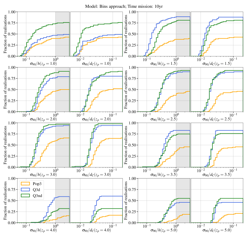
Figure 14: Same as Fig. 7 but for $h(z_{p})$ and $d_{C}(z_{p})$ from the redshift bins approach at different pivot redshifts, according to the x-axis labels. Colors represent different astrophysical models as reported in the legend. The cumulative distributions reach the fraction of informative realisations (see Sec. VI.2): for example at $z_{p}=3.5$, only $\sim 75\%$ of the Q3d and Q3nd realisations provide useful constraints.

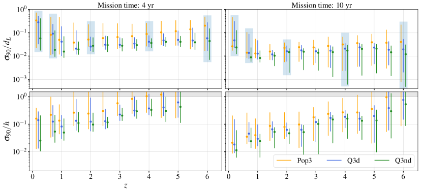
Figure 15: Relative errors at 90% for $d_{L}(z)$ (upper panels) and $h(z)$ (lower panels) as a function of redshift from the splines interpolation model. Error bars also correspond to $90\%$. Light blue boxes highlight the uncertainties at the knot redshifts. To be compared with Fig. 9 but we switched the order of $d_{L}(z)$ and $h(z)$ because the outcomes of the splines are the $d_{L}$ posterior distributions at the knots. To be compared also with Fig. 2 of Bull et al. (2021) but note that they report the uncertainties at $1\sigma$ so our values must be divided by a factor $\sim 1.6$ for proper comparison. Splines can constrain the luminosity distance to $<10\%$ in 4 yr at $1<z<4$ and up to $z\sim 6$ in 10 yr of observations.

VIII Discussions and conclusions

In this paper we provide forecasts on LISA ability to constrain the expansion of the Universe, combining the luminosity distance information from the GW signal of MBHBs with the redshift, obtained from the identification of the host galaxy. We built this paper following the results of M22 Mangiagli et al. (2022) where we estimated the number of EMcps, i.e. systems for which we have a detectable EM counterpart and a sufficiently good sky localization. Since these sources provide independent estimates on $d_{L}$ and $z$, they can be considered as standard sirens, perfect tools for cosmological tests. The additional advantage of MBHBs is that we expect to detect their EM counterpart up $z\sim 7-8$, which means that we can use these systems to test the expansion of the Universe at intermediate redshifts $2\lesssim z\lesssim 8$.

Starting with 90 years of simulated data, we generated 100 realisations of our Universe for three astrophysical models, assuming 4-year and 10-year mission durations. For each event, we convolved the $d_{L}$ posterior distributions from the LISA data analysis process with the expected errors from lensing and peculiar velocities. Regarding the redshift error, we assumed a Gaussian distribution. We split the analysis in ‘Local Universe’ models where we focused on local measurements, as the Hubble constant at $z=0$, and in ‘High-redshift Universe’ models where we explored LISA abilities to put constraints on $h(z)$ with $z\gtrsim 2$. For each model, we performed the Bayesian inference of the corresponding cosmological parameters and we combined the 100 realisations to provide realistic forecasts of LISA capabilities.

As a general trend, we find that LISA will likely not provide estimates on $h$ and $\Omega_{m}$ competitive with future EM measurements due to the limited number of expected EMcps. For instance, assuming $\Lambda$CDM, LISA will constrain $h$ with a relative error of less than $5\%$ in 4 years and less than $2\%$ in 10 years, while $\Omega_{m}$ is constrained with an accuracy of only $10\%$ in 10 years. If the Hubble tension remains unresolved by around 2040, LISA observations of MBHBs can potentially shed light on the true value of $h$, addressing one of cosmology’s long-standing challenges. LISA will also not be particularly sensitive to deviations in the dark energy equation of state: assuming the standard CPL formalism to describe dark energy, we found constraints on $\omega_{0}$ greater than $30-40\%$ in almost all cases and no constraining power on $\omega_{a}$. However, LISA can test alternative gravity theories where GWs do not propagate as photons even if they have the same speed Belgacem et al. (2019): we found that MBHBs-only observations can constrain $\Xi_{0}$ to $<10\%$ in just 4 yr.

The detection of the EM counterparts from MBHBs up to $z\lesssim 8$ gives us the possibility to test the expansion of the Universe in a still unmapped range. As MBHBs can only be observed with LISA, this represents a unique science case for the mission. To fully assess LISA capabilities, we investigated four ‘High-redshift Universe’ models to constrain the matter equation of state or the value of the Hubble parameter at certain pivot redshifts.

In the $(h,\Omega_{m},\beta)$ model we tested LISA ability to determine the matter equation of state, assuming $\omega_{m}=\beta$. LISA constrains $\beta$ within $10\%$ ($20\%$) in 10 yr (4 yr) of observations. However, in this analysis, we also discovered that LISA has no constraining power on $\Omega_{m}$ due to its degeneracy with $\beta$.

In the matter-only approximation we assumed that the Universe is matter-dominated and we defined a $d_{L}-z$ relation with $h(z_{p})$ and $d_{C}(z_{p})$ as unknown parameters. We found that $h(z_{p}=2)$ can be constrained at $3-5\%$ in 10 yr while $h(z_{p}=3)$ is constrained with an accuracy $<10\%$ in the same time interval. For the comoving distance we expect few percent precision in almost all cases.

In the redshift bins model we interpolated $d_{L}(z)$ as a straight line around a pivot redshift $z_{p}$. The advantage of this approach is that we do not assume a functional form for $h(z)$ (the only assumption at the level of the luminosity distance is that the Universe is flat) but only the EMcps falling in a given redshift bin can be considered in the analysis. The simple nature of the cosmological model (c.f. for example with the $\Lambda$CDM where $h(z)$ is expressed as in Eq. 8) and the smaller fraction of EMcps available for the analysis required a more thoughtful approach to avoid results that would have been dominated by priors. In order to identify the informative realisations, we computed the JS divergence between the posterior and the prior distributions of $h(z_{p})$ and we retained only the realisations with $\rm JS>0.5$ . Following this procedure, the largest number of informative realisations is achieved at $z_{p}=3$ because it is where the distribution of the EMcps peaks in redshift. However, the constraints on $h(z_{p}=3)$ are only at $\sim 20\%$. At lower redshift we still have a similar precision in the recovered values of $h(z_{p})$ because $d_{L}$ and $z$ errors are smaller but the number of informative realisations decrease due to the lack of sources. At higher redshifts $(z_{p}>3.5)$ the lack of EMcps and the larger errors lead naturally to a decrease of the informative realisations and to worse constraints on $h(z_{p})$.

The key results of this work are presented in the splines interpolation model where we fit the $d_{L}-z$ relation with cubic splines polynomials from $z=0$ up to $z=7$. The outcomes of the analysis are the $d_{L}$ posterior distributions at 5 knots redshifts that can be used directly to determine the luminosity distance or, if the derivative is computed, the Hubble parameter at any redshift. In this model, we recover the luminosity distance with an error of $<10\%$ up to $z\sim 6$ with 10 yr of data, a forecast competitive with future EM-only observations.

During the realisation of this manuscript, we also tested additional models. Most of them predict a $d_{L}-z$ relation different from $\Lambda$CDM. Since our data are constructed according to the $\Lambda$CDM model, we can make predictions only assuming this cosmology or any extension of it; any alternative cosmology leads to systematic biases in the recovered parameters. In particular, we tested:

1. A phenomenological expression where the luminosity distance is approximated by a third-order polynomial expansion Risaliti and Lusso (2019). The expected $d_{L}-z$ relation is close to $\Lambda$CDM at small redshift but but deviates at $z>2$, resulting in systematic biases in the recovered $h$. For this case, we also attempted to expand the luminosity distance in redshift (scale factor) around a general pivot redshift (scale factor) but with no success.

2. A phenomenological tracker model Bull et al. (2021) where the dark energy equation of state undergoes a smooth transition, parameterised by four additional parameters. This model aroused our interest because the transition might happen in the matter-dominated era, at $1<z<7$. However the large number of parameters (6 = 4 + $h$ + $\Omega_{m}$) and the limited number of EMcps make the model challenging to test with MBHBs.

3. A dark energy model, in which the cosmological constant switches sign at a certain $z_{\dagger}$ due to a transition from an anti-de Sitter to a de Sitter Universe Akarsu et al. (2023). Assuming $\Lambda$CDM, $z_{\dagger}\rightarrow+\infty$, so we were only able to establish lower limits on this parameter. Since it was not particularly informative, we decided to remove it.

4. A vacuum metamorphosis model Parker and Raval (2000); Caldwell et al. (2006) where the Ricci scalar $R$ evolves during cosmic history until a certain $z_{\star}$ where it freezes to $R=m^{2}$, being $m$ the mass of the scalar field. The interest in this model lies in the fact that it is not a phenomenological description but rather a consequence of first principles theory. However, the predicted $d_{L}-z$ relation by this model differs from the $\Lambda$CDM one, leading to strong biases in our estimates.

In this work, we restrict our analyses to MBHBs. However LISA will also observe EMRIs and, at higher frequencies, the early inspiral stellar-mass binary black holes. Both of these populations can in principle be used as dark (or spectral) sirens Del Pozzo et al. (2018); Kyutoku and Seto (2017b); Muttoni et al. (2022); MacLeod and Hogan (2008); Laghi et al. (2021); Liu et al. (2023). We expect LISA constraints to significantly improve when EMRIs and MBHBs are analyzed together Tamanini (2017); Laghi et al. . The former will probe the low-redshift portion of the Universe, while the latter will test the intermediate redshift range. This interplay between the redshift range probed by different LISA source populations will help breaking degeneracies in the $d_{L}(z)$ relation, substantially improving the constraints we found in the present study.

Appendix A Convergence of the realisations

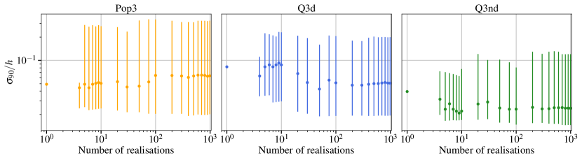
Figure 16: Median relative uncertainty on $h$ as a function of the number of realisations. Errors bars represent the 90 percentile. For all astrophysical models, 100 realisations are sufficient to construct a statistically representative sample.

Since we adopted mock catalogues of MBHB mergers, one important question is how many realisations are necessary in order to provide reliable estimates on the cosmological parameters. If the number of realisations is too small, the results are strongly affected by the Poisson noise, i.e. we might have better or worse estimates respect to the median value, depending on the MBHBs we randomly select. However, we expect that after a sufficiently large number of realisations the average results will not be anymore sensitive to the particular realisations. To answer this question, we generate 900 additional realisations respect to the 100 that were used for the results in the main text, for a total of 1000 realisations. For each of these additional realisations, we performed the inference only in the $(h,\Omega_{m})$ model. In Fig. 16 we show the median relative uncertainty in $h$ and the range of the 90 percentile for the three astrophysical models as a function of the number of realisations. As expected, if we consider $<10$ realisations, the median and 90 percentile values fluctuate by a factor of $\sim 2$. After 100 realisations, the average results stabilise, justifying the choice of 100 realisations that we adopted throughout the entire analysis.

Appendix B Gaussianity of the luminosity distance posteriors

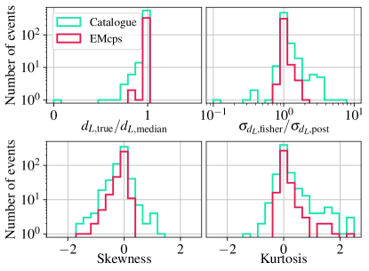
Figure 17: Upper left panel: ratio between the true value of the luminosity distance and the median value from the $d_{L}$ posterior distributions. Upper right panel: ratio between the $1\sigma$ uncertainty from fisher analysis and from $d_{L}$ posterior distribution. Lower left panel: skewness of the $d_{L}$ posteriors. Lower right panel: same as the left one but for the kurtosis. Aquamarine (crimson) lines correspond to the distribution for the entire catalogues (the subset of EMcps). This plot is only for the Q3d model. Overall, the $d_{L}$ posterior distributions for the EMcps can be considered as Gaussian distributions.

In this appendix, we discuss the gaussianity of the luminosity distance posterior distributions. This approximation has been extensively used in the past, in all the analysis performed with a fisher matrix (by construction, the fisher matrix ‘assumes’ that the posterior is a Gaussian distribution). Here we check the validity of this approximation.

In Fig. 17, we report:

1. the ratio between the true luminosity distance and the median of the posterior distributions;

2. the ratio between the variance from the fisher and from the posterior distributions;

3. the skewness of the luminosity distance posterior distributions;

4. the kurtosis of the luminosity distance posterior distributions;

for the entire Q3d catalogue and for the subset of EMcps. If we consider the entire population of MBHBs, it is evident that the results from the fisher analysis are not fully compatible with the Bayesian results. However if we consider the sub-population of EMcps, the posterior distributions appear more Gaussian with median values closer to the real luminosity distance and the ratio of the variances peaking at 1. Similarly, also the skewness and the kurtosis are more centered around the zero, as expected from a normal distribution. We obtain similar results for Pop3 and Q3nd.

Appendix C Assessment of the JS convergence statistic

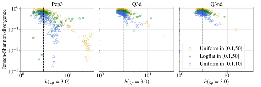
Figure 18: Scatter plot of JS divergence computed between the posterior distribution of $h(z_{p}=3)$ and different priors (as specified in the legend) versus the inferred median value of $h(z_{p}=3)$. The dashed black line represents the value of $h(z_{p}=3)\sim 3.06$, according to $\Lambda$CDM.

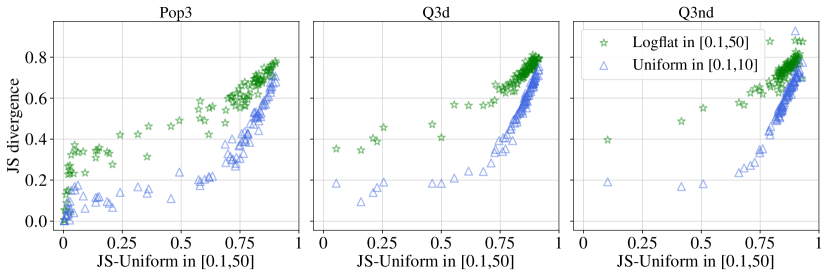
Figure 19: Comparison between JS divergence values from different priors, as stated in the legend. On the x-axis we report the JS divergence adopted in the main text, i.e. with uniform prior in [0.1,50].

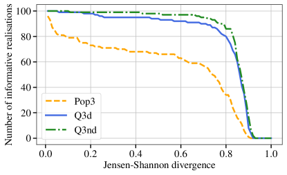
Figure 20: Number of informative realisations as a function of the JS divergence for the three astrophysical models, as in the legend. The JS divergence is computed for $h(z_{p}=3)$ with the prior adopted in the main text.

In this appendix, we present further details on the JS divergence adopted to distinguish between informative and uninformative realisations in the case of the redshift bins approach. As reported in the main text, the value of the JS divergence depends on the choice of the prior adopted. In Fig. 18 we show the JS divergence for three different types of priors:

1. Uniform in $[0.1,50]$;

2. Logflat in $[0.1,50]$;

3. Uniform in $[0.1,10]$.

The first one corresponds to the prior adopted in the analysis in the main text. As expected different priors lead to different JS divergence values. In particular, both the logflat prior and the uniform prior in [0.1,10] present smaller JS divergences. This stems from the fact that in the logflat case we give more weight to small values of $h(z_{p})$, where the true value is. In the uniform case between [0.1,10], the JS values are smaller because the range of the prior is narrower and, therefore, the posteriors look more similar to the priors. Moreover in the uniform case in [0.1,10], we can observe some realisations with low JS divergence and median value $\sim 5$, the midpoint of this prior range. As expected, this subset of systems correspond to the uninformative realisations. From Fig. 18, it is clear that the choice of the threshold for the JS divergence depends on the adopted prior. As discussed in the main text, this value is somewhat arbitrary, and we aim to understand if there is a way to justify or support this choice.

In Fig. 19 we present the scatter plot of the JS divergence in the logflat or in the uniform in $[0.1,10]$ case versus the JS values from the uniform prior in $[0.1,50]$ adopted in the main text. Both cases exhibit a monotonic behavior (with only a few exceptions for Pop3 at small JS values), granting us the possibility to change priors, keeping the same informative realisations. For example, a JS divergence threshold of $0.5$ for the uniform prior in $[0.1,50]$ roughly corresponds to the same value for a logflat prior in $[0.1,50]$. However, if we adopt a uniform prior in $[0.1,10]$, we need to lower the threshold to $\sim 0.2$ to maintain consistency in the analysis and select the same systems. While this comparison allows us to make prediction that are less dependent on the choice of the prior, the open question remains on how to set the “first” threshold. In the main analysis with the uniform prior in $[0.1,50]$, we fixed the JS divergence threshold at $0.5$ in order to eliminate the spurious points with the inferred median values of $h(z_{p})\sim 25$.

Performing the cosmological analysis with different priors and fixing the thresholds following the scaling relations in Fig. 19, we found that the uninformative realisations were always the same, irrespective of the adopted priors. Finally, in Fig. 20 we report the number of informative realisations as a function of the JS threshold for the uniform prior in $[0.1,50]$. As expected, setting a value close to 0 renders all realisations informative, while a value close to 1 makes none of them informative. However, it’s worth noting that there isn’t a ’plateau’ around the value of $0.5$ we adopted, so the presented figures might slightly change with an increase or decrease in the threshold.

Appendix D Pivot parameter for $(h(z),\Omega_{m})$

A set of variables might present some degree of correlation. Therefore, a natural approach is to construct a new set of variables where the correlation is zero. In the context of dark energy, this approach has been adopted by several studies in the past (see Eisenstein et al. (1999) for the original idea and Albrecht et al. (2006) for an application). Assuming the same dark energy expression in Eq. 9, one can search for a pivot redshift $z_{p}$ (or corresponding scale factor $a_{p}$) where the error on $\omega(a)$ is minimized. It can be demonstrated that this redshift corresponds to

$$1-a_{p}=-\frac{\sigma_{\omega_{0}\omega_{a}}}{\sigma_{\omega_{a}}^{2}}$$ (39)

where $\sigma_{\omega_{0}\omega_{a}}$ corresponds to the correlation between $\omega_{0}$ and $\omega_{a}$ and $\sigma_{\omega_{a}}^{2}$ corresponds to the variance for $\omega_{a}$. In order to explain the fact that we have the best constraints on $h(z)$ at $z\sim 0.5$ in Fig. 9, we want to find a redshift for which the correlation between $h(z)$ and $\Omega_{m}$ is minimum. We start defining the variance-covariance matrix between $h$ and $\Omega_{m}$ as

$$\Sigma_{h,\Omega_{m}}=\begin{pmatrix}\sigma_{h}^{2}&\sigma_{hm}\\ \sigma_{hm}&\sigma_{m}^{2}\\ \end{pmatrix}$$ (40)

where $\sigma_{h}^{2}$ ($\sigma_{m}^{2}$) corresponds to the variance for $h$ ($\Omega_{m}$) and $\sigma_{hm}$ is the correlation term. We want to go from the old set of variables $(h,\Omega_{m})$ to the new set formed by $(h(z),\Omega_{m})$ with $z$ that will be specified imposing the minimum correlation. Following the rules for the propagation of errors, we can write the variance-covariance matrix for $(h(z),\Omega_{m})$ as

$$\Sigma_{h(z),\Omega_{m}}=\rm{J}\,\Sigma_{h,\Omega_{m}}\,\rm{J}^{\rm T}.$$ (41)

where $\rm J$ is the Jacobian of the transformation defined as

$$\rm{J}=\begin{pmatrix}\frac{\partial h(z)}{\partial h}&\frac{\partial h(z)}{\partial\Omega_{m}}\\ \frac{\partial\Omega_{m}}{\partial h}&\frac{\partial\Omega_{m}}{\partial\Omega_{m}}\\ \end{pmatrix}.$$ (42)

Performing the calculation, we get

$$\Sigma_{h(z),\Omega_{m}}^{11} =\frac{hz\left(z^{2}+3z+3\right)\left(h\sigma_{m}^{2}z\left(z^{2}+3z+3\right)+4\sigma_{hm}\left(\Omega_{m}z\left(z^{2}+3z+3\right)+1\right)\right)+4\left(\Omega_{m}\sigma_{h}z\left(z^{2}+3z+3\right)+\sigma_{h}\right)^{2}}{4\Omega_{m}z\left(z^{2}+3z+3\right)+4}$$ (43)

$$\Sigma_{h(z),\Omega_{m}}^{12} =\frac{h\sigma_{m}^{2}z\left(z^{2}+3z+3\right)+2\sigma_{hm}\left(\Omega_{m}z\left(z^{2}+3z+3\right)+1\right)}{2\sqrt{\Omega_{m}z\left(z^{2}+3z+3\right)+1}}$$ (44)

$$\Sigma_{h(z),\Omega_{m}}^{22} =\sigma_{m}^{2}$$ (45)

We highlight three points:

1. The element $\Sigma_{h(z),\Omega_{m}}^{22}$ is left unchanged from the transformation as expected because $\Omega_{m}$ remains the same;

2. If we set $z=0$ in $\Sigma_{h(z),\Omega_{m}}^{11}$, we recover the original value of $\sigma_{h}^{2}$;

3. For the term $\Sigma_{h(z),\Omega_{m}}^{12}$, if we insert the value of variance-covariance matrix from the median realisation, we find that the expression has a zero at $z\sim 0.6$, compatible with the results in Fig. 9.