Short-term prediction of construction waste transport activities using AI-Truck

Abstract

Construction waste hauling trucks (or ‘slag trucks’) are among the most commonly seen heavy-duty vehicles in urban streets, which not only produce significant NOx and PM emissions but are also a major source of on-road and on-site fugitive dust. Slag trucks are subject to a series of spatial and temporal access restrictions by local traffic and environmental policies. This paper addresses the practical problem of predicting slag truck activity at a city scale during heavy pollution episodes, such that environmental law enforcement units can take timely and proactive measures against localized truck aggregation. A deep ensemble learning framework (coined AI-Truck) is designed, which employs a soft vote integrator that utilizes BI-LSTM, TCN, STGCN, and PDFormer as base classifiers to predict the level of slag truck activities at a resolution of 1km$\times$1km, in a 193 km² area in Chengdu, China. As a classifier, AI-Truck yields a Macro f1 close to 80% for 0.5h- and 1h-prediction.

I Introduction

According to the World Health Organization (WHO), almost everyone worldwide (99%) is exposed to air that surpasses the recommended WHO guidelines and contains significant levels of pollutants. This issue is particularly severe in lower-middle-income countries, where the population faces the highest levels of exposure. Prolonged exposure to poor air quality can lead to severe health problems [1, 2, 3]. Studies indicate that air pollution has now become the fourth leading cause of death globally. Consequently, there is an urgent imperative to enhance air quality.

Slag trucks are significant contributors to air pollution[4]. On the one hand, as one of the most common heavy-duty diesel vehicles on city roads, they generate substantial amounts of NOx and PM emissions, which are major pollutants. As an example, 25% of the worldwide PM air pollution comes from transportation[5], with heavy-duty diesel vehicles being the primary source of PM emissions[6]. Specifically, in China, heavy-duty vehicles were responsible for over 76% of total vehicle emissions of NOx and over 51% of total vehicle emissions of PM in 2022 [7]. Meanwhile, during the transport of soil and sand, slag trucks also contribute to the generation of fugitive dust[9, 10, 11], which is a major source of atmospheric particulate matter[8]. Last but not least, slag truck aggregation usually indicates ongoing earthworks throughout the city, which are also within the purview of environmental management.

To combat air pollution, local authorities have implemented a range of transportation and environmental policies targeting the use of slag trucks, especially during heavy pollution episodes (HPEs). Specifically, a series of access restrictions are imposed for several key management areas (KMAs) in the city during HPEs. From the standpoint of environmental law enforcement, it is crucial to predict locations with high truck concentration, such that personnel can be dispatched in a timely fashion to collect evidence and administer intervention while on site, thereby enabling proactive measures against environmental deterioration associated with the use of slag trucks.

Driven by this practical challenge, this paper focuses on short-term prediction of the level of slag truck activities on a city scale during HPEs. We present a deep ensemble learning framework called AI-Truck to assist environmental law enforcement, which employs a soft-voting integrator that utilizes BI-LSTM, TCN, STGCN, and PDFormer as the base classifiers. Our work demonstrates its scientific and practical values in the following aspects:

1. This work uses bagging with a voting strategy to synthesize information from multiple independent base classifiers (deep neural networks), which renders more stable prediction results than conventional boosting strategy.

2. Unlike conventional traffic prediction that focuses on link flows or speeds, this work predicts vehicle concentration in a two-dimensional space, which has a unique challenge of data imbalance due to the sparse distribution of truck activities. We address this issue by proposing a combination of down-sampling and weighted loss.

3. Unlike previous work that assumes correlated flows of neighboring grids, we propose an approach based on stay points to determine the correlation between neighboring grids and construct accurate and effective spatial features.

4. In a real-world scenario in Chengdu (China) during the Heavy Pollution Episode in August 2022, our predictions has a Macro f1 score of approximately 80% for both 0.5-hour and 1-hour prediction intervals. AI-Truck can assist local authorities to take timely and effective actions without conducting exhaustive search.

II Related work

Predicting traffic conditions is a challenging task due to the intricate and ever-changing spatio-temporal dependencies present in traffic data[12]. Among the plethora of methods available for traffic prediction, deep neural networks have risen to prominence[13] owing to their remarkable capability to effectively capture intricate and nonlinear traffic patterns[14, 15]. To capture temporal dependence, previous researchers commonly employed recurrent neural networks (RNNs)[16, 17] and temporal convolutional modules (TCNs)[18, 19]. On the other hand, convolutional neural networks (CNNs)[16] were utilized to capture spatial dependency. However, CNNs have certain limitations when applied to regular grid-based traffic data. To address this limitation, graph neural networks (GNNs) have been introduced, offering improved modeling of the inherent graph structure in traffic data[20, 21, 22, 23, 24, 25, 26]. Nevertheless, the spatial dependencies constructed by GNNs are static and localized, lacking consideration for time delays[27]. As a result, researchers have recently shifted towards transformer-based methods to construct spatio-temporal features for traffic prediction[27, 28].

Bootstrap Aggregation, also known as bagging, is a highly effective ensemble method for improving unstable estimates or classifiers, particularly in scenarios involving high-dimensional datasets[29, 30]. The key to the success of bagging methods lies in the utilization of diverse base classifiers that can complement each other effectively[31]. Among the various bagging classification strategies, soft voting and hard voting are widely recognized for their exceptional performance in numerous studies[32, 33, 34, 35]. Soft voting, in particular, offers the advantage of synthesizing information from multiple classifiers, thereby enhancing the model’s robustness.

We observe that existing traffic flow prediction methods primarily estimate vehicle counts at specific locations (e.g. links, subnetworks) and times [12, 36], but there is a lack of prediction regarding the level of vehicle concentration, which is motivated by the slag truck application at hand. While a wide spectrum of deep learning models can effectively learn features from high-dimensional traffic flow data to facilitate prediction, they often encounter the issue of instability [37, 38]. To tackle this challenge, we employ bagging, a technique that adeptly handles high-dimensional data and improves classifier stability [39]. We hypothesize that combining different traffic flow prediction models with bagging techniques can yield promising results, although research in this area is still in the exploratory stage.

III Problem and data description

III-A Problem Definition

We begin by dividing the study area into a set $S$ of 1 km × 1 km spatial grids and set $T$ of 0.5-hr periods. The scope of the study is defined as an element $u=\left(s,t\right)\in S\times T$. The main task of this work is according to $k$ historical slag truck traffic conditions $\left(f^{\tau-k+1},...,f^{\tau}\right)$ observed by the $M$ grids and a traffic network $\mathcal{G}$, using a forecasting model $\mathcal{F}$ to predict the level of slag truck activities at next time step $\left({\hat{c}}^{\tau+2},{\hat{c}}^{\tau+3}\right)$. It is important to note that the next time step we predict starts at ${\hat{c}}^{\tau+2}$, rather than ${\hat{c}}^{\tau+1}$. This adjustment is necessary to allow for a minimum 0.5-hour interval, ensuring that environmental law enforcement units have sufficient time to reach the region where slag trucks concentrate. The prediction problem for the level of slag truck activities is defined as follows:

$$\left({\hat{c}}^{\tau+2},{\hat{c}}^{\tau+3}\right)=\mathcal{F}\left(f^{\tau-k+1},...,f^{\tau},\mathcal{G}\right)$$ (1)

where $f^{\tau}$ denotes the features at moment $\tau$ for predicting the target values. $\hat{c}^{\tau}$ and $c_{m}^{\tau}$ denote the predicted and true level of slag truck activities at moment $\tau$, respectively. The level of slag truck activities $c_{m}^{\tau}$ can be divided into three categories, which are defined as follows:

$$\left\{\begin{aligned} &v_{m}^{\tau}=0,c_{m}^{\tau}=0\\ &0<v_{m}^{\tau}\leq 5,c_{m}^{\tau}=1\\ &v_{m}^{\tau}>5,c_{m}^{\tau}=0\\ \end{aligned}\right.$$ (2)

where $v_{m}^{\tau}$ donates the number of slag trucks in grid $m$ at moment $\tau$.

III-B Trajectory points of slag trucks in chengdu

With the widespread use of GPS in slag trucks, obtaining the trajectory points of slag trucks is no longer a challenging task. Fig. 1 illustrates the full volume trajectory map of slag trucks in Chengdu at a specific moment.

Figure 1: Slag trucks’ stay points in Chengdu at a specific moment.

For our preliminary study, we utilized trajectory point data from all slag trucks in Chengdu during heavy pollution episode from August 3, 2022, 0:00 to August 28, 2023, 23:00. However, not all trajectory points proved useful for predicting the level of slag truck activities. For instance, stationary slag trucks over extended periods have minimal impact on air quality, while managing high-speed trucks poses challenges. Hence, the screening of trajectory points becomes necessary.

We have specifically focused on the trajectory points generated by slag trucks during the loading and unloading process. On the one hand, this is due to this process contributes to the most severe air pollution. The slower speed of slag trucks during loading and unloading results in incomplete fuel combustion, leading to increased emission of air pollutants[40]. Additionally, loading and unloading sites are often characterized by dust, with trucks engaging in these sites generating a significant amount of fugitive dust, further exacerbating air pollution. On the other hand, the slower speeds of slag trucks during loading and unloading make them easier to manage. Therefore, in this paper, we specifically focus on the trajectory points during this period of time, which we refer to as stay points. Stay points are defined as trajectory points where the mileage of an active slag truck does not exceed 200 meters within a 10-minute period. According to the definition of stay points, we apply semantic-based trajectory segmentation[41] for each vehicle, as illustrated in Fig. 2.

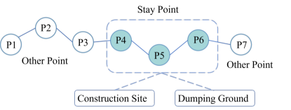
Figure 2: Schematic of semantic segmentation of trajectory points.

We initially chose the Key Management Areas (KMAs) as the primary study regions due to their designation as crucial control zones by the government. These areas are characterized by a high level of activity in terms of slag truck entry and exit. In the case of Chengdu, KMAs have been divided into 1,199 grids, with each grid measuring 1km x 1km, as illustrated in Fig. 3.

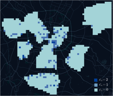
Figure 3: Slag trucks activity levels in Chengdu’s KMAs.

After selecting the study object and study area, we counted the number of slag trucks in each grid with a time granularity of 30 minutes to obtain the level of slag truck activities. The detailed calculation process is described in Algorithm 1. The spatial feature of grid $m$ is denoted by the two-tuple $g_{m}=\left(g_{m}^{br},g_{m}^{tl}\right)\in G$, where $g_{m}^{br}=(\text{lat}_{m}^{br},\text{lon}_{m}^{br})$ and $g_{m}^{tl}=(\text{lat}_{m}^{tl},\text{lon}_{m}^{tl})$ are the coordinates of the bottom right and top left corners of the grid, respectively. Furthermore, the features of stay point $n$ is represented as $p_{n}=\left(l_{n},d_{n},t_{n}\right)\in P$. In this representation, $l_{n}$, $d_{n}$, and $t_{n}$ correspond to the spatial feature of the stay point, the license plate number of the slag truck, and the time when the stay point is generated, respectively. Additionally, the features of slag truck $j$ are denoted by $c_{j}=\left(d_{j},e_{j}\right)\in C$, where $d_{j}$ and $e_{j}$ represent the license plate number and emission standard of the slag truck, respectively.

Algorithm 1 Calculation of the level of slag truck activities

  

  INPUT

       $\textbf{(1) Spatial feature}\ g_{m}=\left(g_{m}^{br},g_{m}^{tl}\right)\in G$

       $\textbf{(2) Stay point features}\ p_{n}=\left(l_{n},d_{n},t_{n}\right)\in P$

       $\textbf{(3) Slag truck features}\ c_{j}=\left(d_{j},e_{j}\right)\in C$

  PROCEDURE

       Step1: Drop the stay points generated by slag

       trucks with emissions standards below National 5

       $\textbf{(1) For }p_{n}\in P$, $c_{j}\in C\textbf{, if }d_{n}==d_{j}\textbf{, then }$

       $p_{n\,\,}=\left(l_{n},d_{n},t_{n},e_{j}\right)$

       $\textbf{(2) If }e_{j}>5\textbf{, drop }p_{n}$

       Step2: Statistical the level of slag truck activities

       (1) Make 30 minutes as the time granularity, for

       $g_{m}\in G\ \textbf{and }p_{n}\in P\textbf{, if }l_{n}\ \textbf{in }g_{m}\textbf{, then }p_{n}\ \textbf{in }g_{m}\textbf{,}$

       $g_{mn}=\left(g_{m}^{br},g_{m}^{tl},d_{n}\right)$

       $\textbf{(2) For }g_{mn}\in G\textbf{, group by }\left(g_{m}^{br},g_{m}^{tl}\right)\textbf{, within the}$

       $\textbf{same group, if multiple}\ g_{mn}\ \textbf{have the same }d_{n}\textbf{, }$

       retain only one of them

       $\textbf{(3) Calculate the number of}\ g_{mn}\ \textbf{in each subgroup }$

       $\textbf{i.e.,}\ v_{m}^{\tau}\textbf{, and obtain the level of slag truck activities }$

       trucks according to function (2)

  OUTPUT

       $\textbf{The level of slag truck activities }c_{m}^{\tau}$

Since slag trucks primarily serve construction sites, it is common for the majority of grids in the target area to be non-occupied, i.e. $c_{m}^{\tau}=0$, as depicted in Fig. 3. Consequently, the level of slag truck activities exhibits a notable sample imbalance, with $a_{m}^{\tau}=1$ accounts for 8.08% of the total samples, while $c_{m}^{\tau}=2$ represents only 1.59% of the total samples. This imbalance leads to the model performing well in predicting samples from the majority class, but it struggles in predicting samples from the minority class.

To tackle the problem of sample imbalance, we employ an under-sampling approach for the grids, retaining only those grids with predictive value. Among all the loading and unloading locations, construction sites contribute the most significant air pollution. Consequently, we identified construction sites as potential study areas within the KMAs region. But we only had access to coordinate information (latitude and longitude) for these construction sites, relying solely on this information to assign them to specific grids would overlook their actual footprint. To account for the possibility of construction sites spanning multiple grids, we also included the eight neighboring grids surrounding each construction site in the alternative study area. However, it is important to note that not all grids necessarily contain construction sites.

We implemented additional selection on the alternative grids to ensure the precise representation of the actual scenario in the grid map. Stay points are generated when slag trucks conduct operations at construction sites, so if there are more stay points in a given grid, it is more likely that a construction site exists in that grid. Consequently, we calculated the average number of stay points for each grid within the alternative study area during the slag trucks control period (21:00 to 7:00 the following day) and removed grids with an average number of stay points below 0.1. This rigorous screening process allowed us to identify grids where construction sites were located.

We have ultimately selected 193 grids as the study area, and their distribution is illustrated in Fig. 4. Although the sample imbalance has been reduced, it still persists. Specifically, $c_{m}^{\tau}=1$ accounts for 27.36% of the total samples, while $c_{m}^{\tau}=2$ accounts for 7.11% of the total samples. The uneven distribution of samples posed a significant challenge in our work.

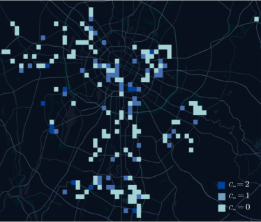
Figure 4: Distribution of slag trucks activity levels after under-sampling.

IV SPATIAL AND TEMPORAL FEATURES

IV-A Spatial Dependence

Effectively capturing spatial dependence enhances prediction accuracy[42]. Traffic flow exhibits spatial connectivity and semantic similarity within space[23], so we construct spatial features from both geographic and semantic perspectives.

IV-A1 Geographic Features

In grid-based traffic maps, there exists a robust correlation between a particular grid and its neighboring grids[43, 44]. As shown in Fig. 5, the flow in grid $g$ is influenced by both the inflow from and outflow to its neighboring grids $g\prime_{m}$. From this observation, it can be inferred that the level of slag truck activities in grid $g$ is also influenced by the level of slag truck activities in its neighboring grids.

Figure 5: Geographic connectivity between neighboring grids.

In previous studies, it has been commonly assumed that all eight neighboring grids $g\prime_{m}$ have spatial dependence on the grid $g$ when constructing the adjacency matrix [16, 27, 43, 45]. However, this approach only yields a pseudo-topology in the constructed adjacency matrix. In reality, the flow out of a grid $g$ is influenced by factors such as roads, resulting in the flow being directed towards only a few specific neighboring grids, rather than all of them. In other words, the grid $g$ does not necessarily exhibit spatial dependence with all eight neighboring grids.

It is worth mentioning that in Section III, we conducted a grid filtering process, resulting in the center grid and its neighboring grids being occupied by the same construction site. As a result, in the graph constructed in this study, the neighboring grids are geographically connected to each other, exhibiting spatial dependence. This allows for the direct construction of the adjacency matrix based on the proximity relationship between the grids.

Eventually, we constructed the adjacency matrix $A$ by taking into account the proximity relationship between the grids, as shown in (3).

$$A\left(i,j\right)=\begin{cases}1,\quad&\text{if}~{}g_{i}~{}\text{and}~{}g_{j}~{}\text{are neighboring}\\ 0,\quad&\text{otherwise}\end{cases}$$ (3)

IV-A2 Semantic Features

Although all the grids within the study area are construction sites, the mode of operation can differ across different construction sites due to factors such as site footprint and construction stage. As a result, the grids demonstrate varying degrees of semantic correlation with each other. To explore the semantic correlation between grids, we utilize the Fast Dynamic Time Warping (FastDTW) approach.

FastDTW is an approximation algorithm for Dynamic Time Warping (DTW) that offers linear time and space complexity[46]. It is widely employed for measuring the similarity between time series data[47, 48]. The core idea of DTW is shown in (4).

$$D\left(i,j\right)= \text{Dist}\left(i,j\right)+\min$$ (4)

$$\big{\{}D\left(i-1,j\right),D\left(i,j-1\right),D\left(i-1,j-1\right)\big{\}}$$

where $\text{Dist}\left(i,j\right)$ represents the first-order relationship between sequences $i$ and $j$.

We computed the semantic matrix $D\left(i,j\right)$ by FastDTW, which represents the degree of semantic correlation between grids. The pseudo-code for exploring semantic correlation is shown in Algorithm 2.

Figure 6: The schema of FastDTW. (a) Time granularity is 4/1. (b) Time granularity is 4/1. (c) Time granularity is 1/1.

Algorithm 2 Exploring semantic correlation among grids

  

  STEP1

       Dividing the time series, we establish the length of

       $\textbf{each subsequence as}\ k\ \textbf{is 48, which corresponds to a }$

       duration of 24 hours

  STEP2

       By setting the time granularity as 1/1, 2/1, and 4/1,

       $\textbf{we divide the original sequence}\ s_{i}\ \textbf{into subsequences }$

       based on the different time granularities

  STEP3

       We calculate the average of each subsequence,

       $\textbf{resulting in three new sequences denoted as}\ s_{i}^{1/1}\textbf{, }$

       $s_{i}^{2/1}\textbf{ and }s_{i}^{4/1}$

  STEP4

       $\textbf{Run \eqref{eq4} for }s_{i4/1}\textbf{ at time granularity of 4/1, as in }$

       Fig. 6(a)

  STEP5

       Obtain path from previous step, it is refined

       temporally to a finer granularity of 2/1 and

       $\textbf{extended outward by additional }q\textbf{ granularities, }$

       $\textbf{where }q=1\textbf{. Then, run \eqref{eq4} for }s_{i2/1}\textbf{ at time }$

       granularity of 2/1, as in Fig. 6(b)

  STEP6

       Repeat STEP3, but this time set the time

       granularity to 1/1, as in Fig. 6(c)

  STEP7

       $\textbf{The final }D\left(i,j\right)\textbf{ represents the degree of semantic }$

       correlation of the grids

IV-B Temporal Dependence

Temporal proximity and periodicity are two crucial components of the temporal relationship in traffic conditions[49]. They play a significant role in predicting traffic patterns, with periodicity being widely regarded as one of the most influential factors[50].

IV-B1 Temporal Proximity

Due to the dynamic nature of the transportation system, the timestamps that are closer to each other tend to exhibit higher similarity compared to timestamps that are further apart[45]. This phenomenon is commonly referred to as temporal proximity.

We calculated the total hourly level of slag truck activities by summing the level of slag truck activities in individual grids. Fig. 7 shows the trend in the total level of slag truck activities on a specific day, highlighting the high degree of similarity that exists in the level of slag truck activities between neighboring timestamps.

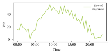
Figure 7: Temporal proximity of the level of slag truck activities.

To capture the temporal proximity in the level of slag truck activities, we employ a sliding window technique[51] with a window size of $k=12$. For a schematic representation of the sliding window, please refer to Fig. 8.

Figure 8: Sliding window schematic.

IV-B2 Temporal Periodicity

A desirable model that effectively captures periodicity can accurately predict future traffic conditions[50]. Fig. 9 depicts the trend in the sum of slag truck activity levels over three consecutive weeks during the study period. The graph demonstrates that the level of slag truck activities exhibits noticeable daily and weekly periodicity. However, unlike other traffic flows, there is no discernible difference in the operating pattern of slag trucks between weekdays and weekends, as construction sites remain active throughout the week. Moreover, the operating pattern of slag trucks exhibits a high level of volatility. This can be attributed to the increased susceptibility of slag trucks to external factors, which presents a challenge in our work.

Figure 9: Temporal periodicity of the level of slag truck activities.

To analyze the daily and weekly periodicity, we extracted the information $h$ and $w$ from the timestamps, representing the hour of the day and the day of the week, respectively.

In summary, the expression for the spatio-temporal feature at a specific point in time $\tau$ is shown as follows:

$$f_{s}^{\tau} =\left(A,D\right)$$ (5)

$$f_{t}^{\tau} =\left(c_{m}^{\tau},h^{\tau},k^{\tau}\right)$$ (6)

$$f^{\tau} =\left(f_{t}^{\tau},f_{s}^{\tau}\right)$$ (7)

where $f_{s}^{\tau}$, $f_{t}^{\tau}$, and $f^{\tau}$ represent the spatial, temporal, and spatio-temporal features, respectively.

V Deep Ensemble Learning for Slag Truck Activity Level

We chose BI-LSTM, TCN, STGCN, and PDFormer as the base classifiers, which are renowned models for traffic flow prediction at various stages of development. These models employ different types of neural networks and are based on different underlying principles[20, 27, 52, 53]. Their diversity and variability align well with the requirements of bagging for base classifiers.

Once the base classifiers are selected, we use soft vote integrator to aggregate the output $\hat{c}_{m}^{\prime}$ of each base classifier, following the aggregation principle shown in (8).

$$\hat{c}_{m} =w_{0}^{\prime}\times\hat{c}_{m}^{\left(BI-LSTM\right)}+w_{1}^{\prime}\times\hat{c}_{m}^{\left(TCN\right)}$$ (8)

$$+w_{2}^{\prime}\times\hat{c}_{m}^{\left(STGCN\right)}+w_{3}^{\prime}\times\hat{c}_{m}^{\left(PDFormer\right)}$$

where $w_{i}^{\prime}$ is the weight of the base classifier, which we set to either 0 or 1 to allow the voter to selectively filter out certain base classifiers. Fig. 10 shows the framework of the model.

Figure 10: A framework for the AI-Truck model.

Despite employing the under-sampling method during the data processing phase to address the issue of slag truck data, sample imbalance remains a challenge. To mitigate the impact of sample imbalance on the model and achieve a balanced prediction effect for both majority and minority samples, we have implemented a weighting approach in the computation of the loss function. By assigning distinct weights to different activity levels, we prioritize the minority samples, giving them greater influence during loss calculation. This enhances the model’s predictive accuracy for the minority samples. The loss function utilized in the model is depicted in (9).

$$\text{loss}=-\sum_{i=0,1,2}{w_{i}\times\log\left(p_{i}\right)}$$ (9)

where $w_{i}$ and $p_{i}$ represent the weights and probabilities, respectively, for activity level $i$.

VI Experiment Results

VI-A Experimental Settings

To evaluate the model’s prediction ability, we divided the slag truck data into a training set and a test set, following an 8:2 ratio. Furthermore, we utilized data from the preceding 6 hours (12-time steps) to predict the level of slag truck activities in the grid after a 0.5-hour interval (14th time step) and a 1.0-hour interval (15th time step).

All experiments were conducted on a machine equipped with an NVIDIA GeForce 4060 GPU and an Intel(R) Core(TM) i9-13900HX CPU. The AI-Truck model was implemented using Windows 11, PyTorch 1.13.1, and Python 3.7. We performed an extensive search for the weights of the loss function and soft vote integrator, and the model was optimized when $\left(w_{0},w_{1},w_{2}\right)=\left(0.4,0.95,1.75\right)$, and $\left(w_{0}^{\prime},w_{1}^{\prime},w_{2}^{\prime},w_{3}^{\prime}\right)=\left(1,0,0,1\right)$ (time interval of 0.5h), and $\left(w_{0}^{\prime},w_{1}^{\prime},w_{2}^{\prime},w_{3}^{\prime}\right)=\left(1,0,1,1\right)$ (time interval of 1h). We trained our model using the Adam optimizer with a batch size of 16 and a training epoch of 200.

VI-B Evaluation Metrics

In practical scenarios, environmental law enforcement units typically focus on the location of construction sites when taking timely and proactive measures against locations with high truck concentrations. Considering that neighboring grids are typically associated with the same construction site, we account for the possibility of prediction mismatches when evaluating the accuracy of sample predictions. Specifically, if a grid’s level of slag truck activities is predicted to belong to category $i$, we consider the prediction to be correct if either the level of slag truck activities on that grid or its neighboring grids also falls into category $i$.

Based on the aforementioned definition of forecast accuracy, we use three metrics in the experiments: Precision, Recall, F1 score, and Macro f1.

VI-C Performance Comparison

We conducted a performance comparison between the AI-Truck model and a base model (BI-LSTM, TCN, STGCN, PDFormer), and the results are presented in Table I and Table II. The best-performing results are indicated in bold, while the second-best results are underlined. Figure 11 displays the confusion matrix of the AI-Truck model on the test data, where Class 0, Class 1, and Class 2 represent the level of slag truck activities $c_{m}=0$, $c_{m}=1$, and $c_{m}=2$, respectively.

TABLE I: Performance of different models at a prediction interval of 0.5h.

Model	Precision			Recall			F1 score			Marco f1
	$c_{m}=2$	$c_{m}=1$	$c_{m}=0$	$c_{m}=2$	$c_{m}=1$	$c_{m}=0$	$c_{m}=2$	$c_{m}=1$	$c_{m}=0$
AI-Truck	0.773	0.771	0.964	0.732	0.835	0.893	0.752	0.801	0.927	0.8267
BI-LSTM	0.734	0.750	0.960	0.707	0.842	0.897	0.720	0.793	0.928	0.8137
TCN	0.716	0.763	0.958	0.749	0.815	0.919	0.732	0.788	0.938	0.8193
STGCN	0.794	0.766	0.971	0.654	0.822	0.800	0.718	0.793	0.877	0.7960
PDFormer	0.741	0.766	0.959	0.712	0.835	0.913	0.726	0.799	0.936	0.8203

TABLE II: Performance of different models at a prediction interval of 1h.

Model	Precis			Recall			F1 score			Marco f1
	$c_{m}=2$	$c_{m}=1$	$c_{m}=0$	$c_{m}=2$	$c_{m}=1$	$c_{m}=0$	$c_{m}=2$	$c_{m}=1$	$c_{m}=0$
AI-Truck	0.703	0.744	0.955	0.678	0.824	0.882	0.690	0.782	0.918	0.7967
BI-LSTM	0.678	0.718	0.954	0.645	0.839	0.860	0.661	0.774	0.905	0.7800
TCN	0.663	0.730	0.953	0.686	0.805	0.884	0.659	0.766	0.918	0.7810
STGCN	0.656	0.752	0.960	0.693	0.774	0.821	0.674	0.763	0.885	0.7740
PDFormer	0.643	0.724	0.959	0.718	0.850	0.854	0.679	0.782	0.903	0.7880

Figure 11: Confusion matrix. (a) Prediction interval of 0.5h. (b) Prediction interval of 1h.

Based on this Table I, Table II and Fig. 11, we can draw the following conclusions:

1. AI-Truck demonstrates a relatively good prediction of the level of slag truck activities, with Macro f1 being approximately 80% for both prediction intervals of 0.5h and 1h. Furthermore, as the prediction time interval increases, the prediction accuracy of AI-Truck remains consistently stable, highlighting its strong robustness.

2. The AI-Truck model, employing the bagging strategy, demonstrates superior performance compared to other base classifiers, providing compelling evidence for the effectiveness of bagging in enhancing predictive accuracy.

3. Among the base classifiers, the PDFormer stands out as the optimal choice. This is attributed to its ability to effectively capture a wide range of features, including geographic features, semantic features, temporal proximity features, and temporal periodicity features. In contrast, the other models only consider a limited number of these features.

4. STGCN exhibits the poorest performance among all base classifiers when the prediction interval is 0.5h. However, in the AI-Truck, we did not assign a weight of 0 to STGCN. The effectiveness of bagging depends not only on the individual performance of each base classifier but also on their complementarity. In this specific case, there is a notable complementarity between BI-LSTM, STGCN, and PDFormer, which contributes to their combined effectiveness.

VI-D Case study

Figure 12: Comparison of projected versus real situation. (a) Predictions for a time interval of 0.5h. (b) The real situation with a time interval of 0.5h. (c) Predictions for a time interval of 1h. (d) The real situation with a time interval of 1h. (e) Consistency at time intervals of 0.5h. (f) Consistency at time intervals of 1h.

In this section, we showcase the prediction results of the AI-trucks on a real traffic map and conduct a comparative analysis with the actual situation. Based on the results of our analysis, we have also provided recommendations to environmental law enforcement units on how to effectively take timely and proactive measures against locations with high truck concentrations.

Fig. 12(a)-(c) respectively display AI-Truck’s predicted classes, true classes, and level of agreement ($A$- difference by two categories, $B$-difference by one category, $C$-agreement), for 0.5h prediction. Fig. 12(d)-(f) display the same quantity for 1.0h prediction. Based on these results, we draw the following conclusions and provide corresponding recommendations:

1. The AI-Truck provides more reliable predictions for the grid in the downtown area compared to other areas. This is largely due to the more regularity of the slag trucks serving the downtown area. The high volume of vehicles in the downtown area during the day makes it challenging for slag trucks to access, resulting in their increased activity primarily occurring at night when the traffic is reduced. In contrast, trucks serving other areas are not constrained by roadway conditions and exhibit a higher degree of randomness in their activity patterns. Therefore, when the predictions indicate a high level of slag truck activities in a downtown grid during nighttime, environmental law enforcement units should prioritize taking timely and proactive measures against locations with high truck concentrations.

2. In the forecasting process, there are instances where the same traffic class occurs simultaneously on two or more neighboring grids. This occurrence typically carries a high level of confidence, as neighboring grids usually belong to the same site and exhibit a similar demand for slag trucks. Environmental law enforcement units can prioritize checks of grids where this condition is observed.

3. The model demonstrates higher reliability when it comes to isolated grids, specifically small construction sites. This can be attributed to the relatively stable demand for slag trucks at these sites. However, due to the lower overall demand for slag trucks at small construction sites, the model’s reliability in predicting high activity levels is not as strong. Therefore, when low activity levels are predicted for slag trucks in isolated grids, environmental law enforcement units can prioritize checks of grids where this condition is observed.

4. Predictions made with a 1-hour time interval are slightly less accurate compared to predictions made with a 0.5-hour time interval. As a result, environmental law enforcement units should take into account both the accuracy of the prediction and the proximity of the current location to a grid with the high level of slag truck activities. It is advisable to prioritize the nearby high activity level grids and choose the closest one as the destination.

VII Conclusion

In this paper, we present an ensemble deep learning framework called AI-Truck, which utilizes a bagging strategy to predict the level of slag truck activities on grids. Our framework utilizes the predictive power of BI-LSTM, TCN, STGCN, and PDFormer as base classifiers and soft vote integrator. Our model effectively captures both temporal and spatial dependencies, including geographic features, semantic features, temporal proximity features, and temporal periodicity features. This comprehensive approach allows us to accurately predict the level of slag truck activities. One of the key challenges we addressed is the uneven sample distribution across the three types of the level of slag truck activities. Despite significant differences in sample sizes, our model consistently produces reliable predictions. This demonstrates the robustness of our framework in handling imbalanced datasets. Furthermore, we have made significant progress in predicting traffic flow categories, achieving promising results. To enhance interpretability, we have mapped the predicted and actual results onto real traffic maps. Based on the results of the visualization, we provide recommendations for environmental law enforcement units to take timely and proactive measures against locations with high truck concentrations.

Overall, our AI-Truck framework offers a powerful solution for predicting the level of slag truck activities on grids. Its ability to capture temporal and spatial dependencies, handle imbalanced datasets, and provide interpretable results makes it a valuable tool for taking timely and proactive measures against locations with high truck concentrations.

As part of our future work, we plan to enhance AI-Truck by integrating additional base classifiers and extracting a broader range of spatio-temporal features from the data. This will further improve the accuracy and robustness of our predictions. Additionally, we aim to apply AI-Truck in a wider range of scenarios that necessitate the prediction of traffic flow categories. By doing so, we can explore its potential in various real-world applications and validate its effectiveness across different contexts.

References

- [1] M. Kampa and E. Castanas, “Human health effects of air pollution,”Environmental polllution, vol. 151, no. 2, pp. 362–367, 2008.
- [2] B. Brunekreef and S. T. Holgate, “Air pollution and health,” The lancet, vol. 360, no. 9341, pp. 1233–1242, 2002.
- [3] J. A. Bernstein, N. Alexis, C. Barnes, I. L. Bernstein, A. Nel, D. Peden, D. Diaz-Sanchez, S. M. Tarlo, and P. B. Williams, “Health effects of air pollution,” Journal of allergy and clinical immunology, vol. 114, no. 5, pp. 1116–1123, 2004.
- [4] X. Deng, “Economic costs of motor vehicle emissions in china: a case study,” Transportation Research Part D: Transport and Environment, vol. 11, no. 3, pp. 216–226, 2006.
- [5] F. Karagulian, C. A. Belis, C. F. C. Dora, A. M. Prüss-Ustün, S. Bonjour, H. AdairRohani, and M. Amann, “Contributions to cities’ ambient particulate matter (pm): A systematic review of local source contributions at global level,” Atmospheric environment, vol. 120, pp. 475–483, 2015.
- [6] P. Jiang, X. Zhong, and L. Li, “On-road vehicle emission inventory and its spatio-temporal variations in north china plain,” Environmental Pollution, vol. 267, p. 115639, 2020.
- [7] Ministry of Ecology and Environment of China, “China mobile source environmental management annual report”, 2022.
- [8] H. Wang, L. Han, T. Li, S. Qu, Y. Zhao, S. Fan, T. Chen, H. Cui, and J. Liu. Temporal-spatial distributions of road silt loadings and fugitive road dust emissions in beijing from 2019 to 2020. Journal of Environmental Sciences, 132:56-70, 2023.
- [9] Y. Ma, M. Gong, H. Zhao, and X. Li. Contribution of road dust from low impact development (lid) construction sites to atmospheric pollution from heavy metals. Science of The Total Environment, 698:134243, 2020.
- [10] H. Yan, G. Ding, K. Feng, L. Zhang, H. Li, Y. Wang, and T. Wu, “Systematic evalua-tion framework and empirical study of the impacts of building construction dust on the surrounding environment,” Journal of Cleaner Production, vol. 275, p. 122767, 2020.
- [11] S. Yang, J. Liu, X. Bi, Y. Ning, S. Qiao, Q. Yu, and J. Zhang, “Risks related to heavy metal pollution in urban construction dust fall of fast-developing chinese cities,” Ecotoxicology and Environmental Safety, vol. 197, p. 110628, 2020.
- [12] X. Yin, G. Wu, J. Wei, Y. Shen, H. Qi, and B. Yin, “Deep learning on traffic prediction: Methods, analysis, and future directions,” IEEE Transactions on Intelligent Transportation Systems, vol. 23, no. 6, pp. 4927–4943, 2021.
- [13] D. A. Tedjopurnomo, Z. Bao, B. Zheng, F. M. Choudhury, and A. K. Qin, “A survey on modern deep neural network for traffic prediction: Trends, methods and challenges,” IEEE Transactions on Knowledge and Data Engineering, vol. 34, no. 4, pp. 1544–1561, 2020.
- [14] W. Huang, G. Song, H. Hong, and K. Xie, “Deep architecture for traffic flow prediction: Deep belief networks with multitask learning,” IEEE Transactions on Intelligent Transportation Systems, vol. 15, no. 5, pp. 2191–2201, 2014.
- [15] H. Yu, Z. Wu, S. Wang, Y. Wang, and X. Ma, “Spatiotemporal recurrent convolutional networks for traffic prediction in transportation networks,” Sensors, vol. 17, no. 7, p. 1501, 2017.
- [16] J. Zhang, Y. Zheng, and D. Qi, “Deep spatio-temporal residual networks for citywide crowd flows prediction,” in Proceedings of the AAAI conference on artificial intelligence, vol. 31, no. 1, 2017.
- [17] H. Yao, F. Wu, J. Ke, X. Tang, Y. Jia, S. Lu, P. Gong, J. Ye, and Z. Li, “Deep multiview spatial-temporal network for taxi demand prediction,” in Proceedings of the AAAI conference on artificial intelligence, vol. 32, no. 1, 2018.
- [18] A. Borovykh, S. Bohte, and C. W. Oosterlee, “Conditional time series forecasting with convolutional neural networks,” arXiv preprint arXiv:1703.04691, 2017.
- [19] S. Bai, J. Z. Kolter, and V. Koltun, “An empirical evaluation of generic convolutional and recurrent networks for sequence modeling,” arXiv preprint arXiv:1803.01271, 2018.
- [20] B. Yu, H. Yin, and Z. Zhu, “Spatio-temporal graph convolutional networks: A deep learning framework for traffic forecasting,” arXiv preprint arXiv:1709.04875, 2017.
- [21] Z. Wu, S. Pan, G. Long, J. Jiang, X. Chang, and C. Zhang, “Connecting the dots: Multivariate time series forecasting with graph neural networks,” in Proceedings of the 26th ACM SIGKDD international conference on knowledge discovery & data mining, 2020, pp. 753–763.
- [22] Z. Wu, S. Pan, G. Long, J. Jiang, and C. Zhang, “Graph wavenet for deep spatial-temporal graph modeling,” arXiv preprint arXiv:1906.00121, 2019.
- [23] Z. Fang, Q. Long, G. Song, and K. Xie, “Spatial-temporal graph ode networks for traffic flow forecasting,” in Proceedings of the 27th ACM SIGKDD conference on knowledge discovery & data mining, 2021, pp. 364–373.
- [24] J. Choi, H. Choi, J. Hwang, and N. Park, “Graph neural controlled differential equations for traffic forecasting,” in Proceedings of the AAAI Conference on Artificial Intelligence, vol. 36, no. 6, 2022, pp. 6367–6374.
- [25] Y. Li, R. Yu, C. Shahabi, and Y. Liu, “Diffusion convolutional recurrent neural network: Data-driven traffic forecasting,” arXiv preprint arXiv:1707.01926, 2017.
- [26] S. Guo, Y. Lin, N. Feng, C. Song, and H. Wan, “Attention based spatial-temporal graph convolutional networks for traffic flow forecasting,” inProceedings of the AAAI conference on artificial intelligence , vol. 33, no. 01, 2019, pp. 922–929.
- [27] J. Jiang, C. Han, W. X. Zhao, and J. Wang, “Pdformer: Propagation delay-aware dynamic long-range transformer for traffic flow prediction,” arXiv preprint arXiv:2301.07945, 2023.
- [28] W. Chen, L. Chen, Y. Xie, W. Cao, Y. Gao, and X. Feng, “Multi-range attentive bicomponent graph convolutional network for traffic forecasting,” in Proceedings of the AAAI conference on artificial intelligence , vol. 34, no. 04, 2020, pp. 3529–3536.
- [29] P. Bühlmann and B. Yu, “Analyzing bagging,” The annals of Statistics, vol. 30, no. 4, pp. 927–961, 2002.
- [30] Z.-H. Zhou, Machine learning. Springer Nature, 2021.
- [31] L. I. Kuncheva and C. J. Whitaker, “Measures of diversity in classifier ensembles and their relationship with the ensemble accuracy,” Machine learning, vol. 51, pp. 181–207, 2003.
- [32] H. B. Mitchell and P. A. Schaefer, “A “soft” k-nearest neighbor voting scheme,” International journal of intelligent systems, vol. 16, no. 4, pp. 459–468, 2001.
- [33] Z. Xu, M. Bashir, W. Zhang, Y. Yang, X. Wang, and C. Li, “An intelligent fault diagnosis for machine maintenance using weighted soft-voting rule based multi-attention module with multi-scale information fusion,” Information Fusion, vol. 86, pp. 17–29, 2022.
- [34] Q. Zhou and H. Wu, “Nlp at iest 2018: Bilstm-attention and lstm-attention via soft voting in emotion classification,” in Proceedings of the 9th workshop on computational approaches to subjectivity, sentiment and social media analysis, 2018, pp. 189–194.
- [35] S. Kumari, D. Kumar, and M. Mittal, “An ensemble approach for classification and prediction of diabetes mellitus using soft voting classifier,” International Journal of Cognitive Computing in Engineering, vol. 2, pp. 40–46, 2021.
- [36] E. I. Vlahogianni, M. G. Karlaftis, and J. C. Golias, “Short-term traffic forecasting: Where we are and where we’re going,” Transportation Research Part C: Emerging Technologies, vol. 43, pp. 3-19, 2014.
- [37] R. Yu, Y. Li, C. Shahabi, U. Demiryurek, and Y. Liu, “Deep learning: A generic approach for extreme condition traffic forecasting,” in Proceedings of the 2017 SIAM international Conference on Data Mining. SIAM, 2017, pp. 777-785.
- [38] H. Xu and C. Jiang, “Deep belief network-based support vector regression method for traffic flow forecasting,” Neural Computing and Applications, vol. 32, pp. 2027-2036, 2020.
- [39] L. Breiman, “Bagging predictors,” Machine learning, vol. 24, pp. 123-140, 1996.
- [40] D. R. Gentner, D. R. Worton, G. Isaacman, L. C. Davis, T. R. Dallmann, E. C. Wood, S. C. Herndon, A. H. Goldstein, and R. A. Harley, “Chemical composition of gas-phase organic carbon emissions from motor vehicles and implications for ozone production,”Environmental Science & Technology, vol. 47, no. 20, pp. 11 837–11 848, 2013
- [41] P. Xie, T. Li, J. Liu, S. Du, X. Yang, and J. Zhang, “Urban flow prediction from spatiotemporal data using machine learning: A survey,” Information Fusion, vol. 59, pp. 1–12, 2020.
- [42] M. Xu, W. Dai, C. Liu, X. Gao, W. Lin, G.-J. Qi, and H. Xiong, “Spatial-temporal transformer networks for traffic flow forecasting,” arXiv preprint arXiv:2001.02908, 2020.
- [43] A. Ali, Y. Zhu, and M. Zakarya, “Exploiting dynamic spatio-temporal graph convolutional neural networks for citywide traffic flows prediction,” Neural networks, vol. 145, pp. 233–247, 2022.
- [44] S. Yang, S. Shi, X. Hu, and M. Wang, “Spatiotemporal context awareness for urban traffic modeling and prediction: sparse representation based variable selection,” PloS one, vol. 10, no. 10, p. e0141223, 2015.
- [45] J. Zhang, Y. Zheng, D. Qi, R. Li, and X. Yi, “Dnn-based prediction model for spatio-temporal data,” in Proceedings of the 24th ACM SIGSPATIAL international conference on advances in geographic information systems, 2016, pp. 1–4.
- [46] S. Salvador and P. Chan, “Toward accurate dynamic time warping in linear time and space,” Intelligent Data Analysis, vol. 11, no. 5, pp. 561–580, 2007.
- [47] T. Rakthanmanon, B. Campana, A. Mueen, G. Batista, B. Westover, Q. Zhu, J. Zakaria, and E. Keogh, “Searching and mining trillions of time series subsequences under dynamic time warping,” in Proceedings of the 18th ACM SIGKDD international conference on Knowledge discovery and data mining, 2012, pp. 262–270.
- [48] O. Maimon and L. Rokach, Data mining and knowledge discovery handbook. Springer, 2005, vol. 2, no. 2005.
- [49] Y. Wu, H. Tan, L. Qin, B. Ran, and Z. Jiang, “A hybrid deep learning based traffic flow prediction method and its understanding,” Transportation Research Part C: Emerging Technologies, vol. 90, pp. 166–180, 2018.
- [50] H. Tan, G. Feng, J. Feng, W. Wang, Y.-J. Zhang, and F. Li, “A tensor-based method for missing traffic data completion,” Transportation Research Part C: Emerging Technologies, vol. 28, pp. 15–27, 2013.
- [51] T. Thianniwet, S. Phosaard, and W. Pattara-Atikom, “Classification of road traffic congestion levels from gps data using a decision tree algorithm and sliding windows,” in Proceedings of the world congress on engineering, vol. 1, 2009, pp. 1–3.
- [52] R. L. Abduljabbar, H. Dia, and P.-W. Tsai, “Unidirectional and bidirectional lstm models for short-term traffic prediction,” Journal of Advanced Transportation, vol. 2021, pp. 1–16, 2021.
- [53] R. Zhang, F. Sun, Z. Song, X. Wang, Y. Du, and S. Dong, “Short-term traffic flow forecasting model based on ga-tcn,” Journal of Advanced Transportation, vol. 2021, pp. 1–13,2021.
- [54] Z. Pan, Y. Liang, W. Wang, Y. Yu, Y. Zheng, and J. Zhang, “Urban traffic prediction from spatio-temporal data using deep meta learning,” in Proceedings of the 25th ACM SIGKDD international conference on knowledge discovery & data mining, 2019, pp. 1720–1730.
- [55] S. M. Abd Elrahman and A. Abraham, “A review of class imbalance problem,” Journal of Network and Innovative Computing, vol. 1, no. 2013, pp. 332–340, 2013.
- [56] S.-J. Yen and Y.-S. Lee, “Cluster-based under-sampling approaches for imbalanced data distributions,” Expert Systems with Applications, vol. 36, no. 3, pp. 5718–5727, 2009.
- [57] E. Chamseddine, N. Mansouri, M. Soui, and M. Abed, “Handling class imbalance in covid-19 chest x-ray images classification: Using smote and weighted loss,” Applied Soft Computing, vol. 129, p. 109588, 2022.
- [58] Y. Wu and H. Tan, “Short-term traffic flow forecasting with spatial-temporal correlation in a hybrid deep learning framework,” arXiv preprint arXiv:1612.01022, 2016.
- [59] M. Li and Z. Zhu, “Spatial-temporal fusion graph neural networks for traffic flow forecasting,” in Proceedings of the AAAI conference on artificial intelligence, vol. 35, no. 5, 2021,pp. 4189–4196.