Urban Region Representation Learning with Attentive Fusion

Abstract

An increasing number of related urban data sources have brought forth novel opportunities for learning urban region representations, i.e., embeddings. The embeddings describe latent features of urban regions and enable discovering similar regions for urban planning applications. Existing methods learn an embedding for a region using every different type of region feature data, and subsequently fuse all learned embeddings of a region to generate a unified region embedding.

However, these studies often overlook the significance of the fusion process. The typical fusion methods rely on simple aggregation, such as summation and concatenation, thereby disregarding correlations within the fused region embeddings.

To address this limitation, we propose a novel model named HAFusion. Our model is powered by a dual-feature attentive fusion module named DAFusion, which fuses embeddings from different region features to learn higher-order correlations between the regions as well as between the different types of region features. DAFusion is generic – it can be integrated into existing models to enhance their fusion process. Further, motivated by the effective fusion capability of an attentive module, we propose a hybrid attentive feature learning module named HALearning to enhance the embedding learning from each individual type of region features. Extensive experiments on three real-world datasets demonstrate that our model HAFusion outperforms state-of-the-art models across three different prediction tasks. Using our learned region embeddings leads to consistent and up to 31% improvements in the prediction accuracy.

I Introduction

Urban region representation learning has recently gained much attention in the field of urban data management [1, 2, 3, 4, 5, 6], which transforms urban regions into vector representations called embeddings. These embeddings yield the correlation of regional functionalities and valuable insights into urban structures and properties. They are valuable in developing innovative solutions to critical urban issues and common problems in daily life [7, 8, 9]. For example, if the manager of a well-run restaurant in a particular region is considering expanding to new locations, utilizing region embeddings can assist in identifying the most comparable regions for this new venture. As the volume of urban data sources continues to grow, it is essential to develop effective methods for region representation learning from rich urban data.

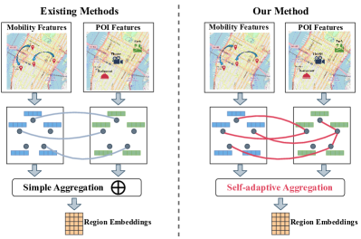
Figure 1: Multi-view fusion region representation learning (each dot denotes a region). Left: existing methods; Right: ours.

Recently, a rising number of studies [10, 11, 12, 13, 14, 15, 16, 17, 18, 19] focus on learning region representations by comparing region correlations from multiple sets of data that describe the same regions (e.g., human mobility and POI data), where each dataset can be considered as depicting the region from a distinct view. For example, two regions may share a similar functionality if they both feature huge human mobility and a large number of entertainment venues.

As Fig. 1 (left sub-figure) shows, existing studies [10, 14, 11, 12] primarily adhere to the following process. Initially, they construct multiple region-based graphs based on distinct sets of data, collectively referred to as multi-view graphs. Subsequently, a view-based embedding is generated from each individual view graph by capturing information of the same region within a single view and across multiple views. Following this, the view-based embeddings are fused to generate a cohesive and unified region embedding.

There are two limitations with the existing studies.

Limitation 1. Existing studies overlook higher-order correlations between regions in the fused embeddings. They often emphasize the generation of more effective view-based embeddings from individual views, neglecting the fusion process. The typical fusion methods leverage simple aggregation, such as summation and concatenation, to fuse multiple view-based embeddings. They overlook higher-order correlations between regions in the fused embeddings, while regions are implicitly interconnected through various types of correlations.

Limitation 2. Existing studies do not consider the correlations of different regions in different views. Existing methods [10, 14] typically learn region correlations in the view-based embedding learning process. As Fig. 1 (left sub-figure) shows, they consider the correlations of different regions in each individual view, and those of the same region in different views (denoted by the blue curves connecting the same region in different views). They do not consider the correlations of different regions in different views.

To address these limitations, we propose a novel model named HAFusion (Fig. 1, right sub-figure), which consists of a dual-feature attentive fusion (DAFusion) module and a hybrid attentive feature learning (HALearning) module.

DAFusion (Section IV-B) has two sub-modules: a view-aware attentive fusion module (ViewFusion) and a region-aware attentive fusion module (RegionFusion). ViewFusion aggregates view-based embeddings from multiple views into one, through the attention mechanism. RegionFusion further captures higher-order correlations between regions from the embeddings that have aggregated information from multiple views, through the self-attention mechanism. By introducing RegionFusion, we can propagate information in the fused region embeddings to encode more comprehensive region correlation information into the final region embeddings. It is important to note that our DAFusion module is generic – it can be integrated with existing models to enhance their fusion process, as shown by our experiments (Section VI-C).

HALearning (Section V), on the other hand, focuses on enhancing the view-based embedding learning process. It captures region correlations in individual views and across views, for both the same region and different regions (denoted by the red curves connecting different regions in different views in the right sub-figure of Fig. 1, with intra-view attentive feature learning (IntraAFL) and inter-view attentive feature learning (InterAFL) modules based on adapted self-attention mechanisms, respectively.

To summarize, this paper makes the following contributions:

• We propose an effective learning model named HAFusion for region representation learning over multiple sets of data for the same region.

• For effective learning, we propose two modules:

  • The hybrid attentive feature learning module computes view-based embeddings that capture region correlations from both individual views and across different views, for both the same region and different regions.

  • The dual-feature attentive fusion module fuses the view-based embeddings while further learning higher-order correlations between the regions from the embeddings that have aggregated information from different views.

• We develop two additional datasets to assess the generalizability of urban region representation learning models, and will release them upon paper publication.

• We conduct extensive experiments to evaluate HAFusion on three real-world datasets. The results demonstrate that HAFusion produces embeddings that yield consistent improvements in the accuracy of downstream urban prediction tasks (crime, check-in, and service call predictions), with an advantage of up to 31% over the state-of-the-art.

II Related Work

Based on whether different types of region features are considered (i.e., each type is a view), region representation learning models can be divided into two categories: single-view learning and multi-view learning.

II-A Single-view Region Representation Learning

We categorize the single-view region representation learning models by the type of region features considered.

Human mobility feature-based. HDGE [20], ZE-Mob [21] and MGFN [22] use human mobility features. HDGE creates two graphs based on human mobility and the spatial similarity between regions, respectively, where regions are the vertices. The human mobility graph uses the trip count from one region to another (recorded over some period) as an edge weight, and the spatial similarity graph uses the inverse of region distance. HDGE then runs random walks on the two graphs to generate sequences of vertices and applies word2vec (i.e., the skip-gram model) [23] to learn region embeddings. ZE-Mob calculates the point-wise mutual information (PMI) between regions by measuring the co-occurrences of regions in the same trip (i.e., as source and destination regions). It learns region embeddings whose dot products approach the PMI values.

MGFN constructs multiple mobility graphs, each with trip counts recorded at a different hour. After that, it clusters the graphs into seven groups according to their time-weighted “distances,” which are defined based on aggregations (e.g., sum) of the edge weights of each graph. All mobility graphs of the same group form a mobility pattern graph. Each mobility pattern graph is then treated as a view, and MGFN learns intra-view and inter-view correlations using the vanilla self-attention mechanism on these graphs to generate region embeddings.

POI feature-based. CDAE [24] and HGI [25] mainly leverage POI features to learn region embeddings. CDAE represents each region as a graph of POIs, where the edge weights are trip counts between the POIs. It uses a collective deep auto-encoder model to learn the POI embeddings over the POI graphs, where are aggregated (weighted sum) as the region embedding. HGI generates embeddings at three hierarchical levels: POI, region (aggregation of POI embeddings), and city (aggregation of region embeddings) levels. It uses a GNN to compute the POI embeddings, which are aggregated to initialise the region embeddings. Another GNN is then used to refine and produce the final region embeddings.

Others. RegionDCL [26] uses building footprints. It partitions the buildings in a region into non-overlapping groups using the road network. The footprint of each building (i.e., an image) is used to compute an embedding with a convolutional neural network (CNN). The building footprint embeddings of a group are aggregated (average) to initialize the embedding of the group. A contrastive learning layer [27] is applied to refine the building group embeddings. The mean of the embeddings of all building groups in a region is the final region embedding. Tile2Vec [28], on the other hand, applies a CNN to learn region embeddings from satellite images directly.

The works above (including our own recent work [29]) except for MGFN use single views and do not require multi-view fusion, which differ from our model structure. Like MGFN, our model HAFusion also uses self-attention. However, we adapt the self-attention mechanism such that the correlation coefficients learned are explicitly (rather than implicitly as done in MGFN) encoded into the region embeddings learned from each view. Further, we learn the correlation between different regions in different views, instead of just the same region in different views as done in MGFN. Thus, we achieve more effective learning outcomes as shown in Section VI.

II-B Multi-view Region Representation Learning

Multi-view region representation learning models [10, 11, 12, 13, 14, 15, 16, 17, 18, 19] incorporate different types (i.e., views) of regions features. Studies [30, 31, 32, 33] have shown that multi-view learning-based models lead to embeddings of a higher quality – they yield higher accuracy on downstream (prediction) tasks. We review these studies based on their view encoders.

Multi-layer perceptron (MLP)-based. MLP-based models include MP-VN [11], CGAL [12], and ReMVC [15].

MP-VN constructs two POI graphs for the POIs in a region. One graph uses POI distances as the edge weights, and the other uses trip counts between POIs. POI embeddings on each graph are randomly initialized and updated with probabilistic propagation-based aggregation [34]. The POI embeddings from both graphs are concatenated into a vector to initialize the region embedding. Then, MP-VN uses an MLP-based autoencoder to learn the latent region embedding. CGAL further introduces two adversarial modules into the autoencoder, which bring in constraints on the learned embeddings, e.g., the cosine similarities of region embeddings should match the region similarity calculated by POI distributions in the regions.

ReMVC is based on self-supervised contrastive learning. It uses an MLP-based encoder to transform region features (e.g., count of POIs in different POI categories) into a latent embedding. Then, it performs contrastive learning on embeddings of the same view, as well as embeddings of different views (for the same region). The embeddings of the same region from different views are concatenated as the final region embedding.

GNN-based. GNN-based models [13, 14, 10, 16] represent regions and their correlations with a graph. For example, DLCL [13] applies a graph convolutional network (GCN) [35] on top of the region embeddings learned from CGAL, to further learn the correlations between the regions.

MVURE [10] also treats regions as vertices. It constructs four graphs using human mobility (source and destination), POI category vector similarity, and POI check-in vector similarity for the edges. It then uses graph attention networks (GAT) [36] to learn embeddings. The final region embeddings are weighted sums of the embeddings from the graphs.

HREP [14] enhances MVURE by replacing the GATs with a relation-aware GCN to learn different relation-specific region embeddings on each graph. Given a downstream task (e.g., crime count prediction), HREP further attaches a task-specific prefix (i.e., a prompt) to the front of each region embedding, which is fine-tuned (i.e., prompt learning) for the task.

HUGAT [16] constructs a heterogeneous graph where the vertices include regions, POIs, POI categories, etc. Then, it applies a heterogeneous GAT [37] to learn region embeddings on the graph, which is effectively a single view-based solution.

Multi-modal-based.. Multi-modal-based models [17, 18, 19] combine numerical features and visual features (e.g., street view images). RegionEncoder [17] uses a GCN and a CNN to jointly learn region embeddings from POIs category count vectors, trip counts, region adjacency data, and satellite images. Urban2Vec [18] and M3G [19] use the triplet loss [38] (similar to contrastive learning) to learn region embeddings from street view images and POI textual descriptions.

Discussion: After embeddings are computed from each view, existing models use simple aggregations, e.g., summation or concatenation, to fuse these embeddings and generate the final region embeddings. In contrast, we propose a self-adaptive fusion module that learns higher-order correlations between the regions as well as between the different types of region features, thus obtaining region embeddings that are more effective for downstream (prediction) tasks.

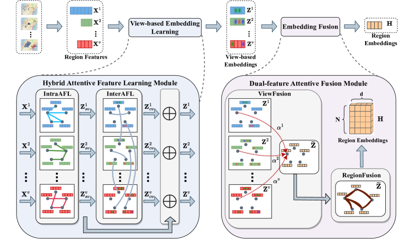
Figure 2: HAFusion model overview. The model takes region feature matrices $\mathbf{X}^{1},\mathbf{X}^{2},\dots,\mathbf{X}^{v}$ (called views) as input and computes region embeddings with two main modules: (1) The hybrid attentive feature learning module computes view-based embeddings ($\mathbf{Z}^{1},\mathbf{Z}^{2},\ldots,\mathbf{Z}^{v}$) for each input view. (2) The dual-feature attentive fusion module further fuses the view-based embeddings at both the view and region perspective to generate the final region embeddings $\mathbf{H}$.

III Preliminaries

We start with a few basic concepts and a problem statement. Frequently used symbols are listed in Table I.

TABLE I: Frequently Used Symbols

3 Symbol	Description
$\mathcal{R}$	A set of regions (non-overlapping space partitions)
$\mathbf{X}^{j}~{}(\mathbf{M},\mathbf{P},\mathbf{L})$	Region feature matrices
$\mathbf{Z}$	View-based region embedding matrix
$\widetilde{\mathbf{Z}}$	Region embedding matrix after ViewFusion
$\mathbf{H}$	Final model output region embedding matrix
3

Region. Regions $\mathcal{R}$ refer to a set of non-overlapping space partitions within a designated area of interest, acquired through a certain partition method (e.g., by census tracts). We consider three types of features for each region to compute their representations as follows.

Human mobility features. Given a set $\mathcal{R}$ of $n$ regions, we define a human mobility matrix $\mathbf{M}$ with a set of human flow records between regions, where $m_{i,j}\in\mathbf{M}$ denotes the number of people moving from region $r_{i}$ to region $r_{j}$ ($r_{i},r_{j}\in\mathcal{R}$) in an observed period of time (e.g., a month or a year as in our experimental datasets, which is orthogonal to our problem definition). We further use $\textbf{m}_{i}$ to denote the vector of outflow records from $r_{i}$ , i.e., $\textbf{m}_{i}=[m_{i,1},m_{i,2},\ldots,m_{i,n}]$. We call it the human mobility feature vector of $r_{i}$.

POI features. Given a region $r_{i}\in\mathcal{R}$, we collect all POIs in $r_{i}$ from OpenStreetMap [39] and extract the POI categories. We consider 26 categories (e.g., restaurants, schools, etc.) following a previous study [29] and count the number of POIs in each category, resulting in a 26-dimensional POI feature vector $\mathbf{p}_{i}$. Such vectors of all $n$ regions form a POI matrix $\mathbf{P}$.

Land use features. The land use features share a similar setup with the POI features. Given a region $r_{i}$, we count the number of zones in $r_{i}$ that fall into different zone categories, e.g., industrial zones, residential zones, or transportation zones. These counts together form the land use feature vector $\mathbf{l}_{i}$ of $r_{i}$. The land use feature vectors of all $n$ regions form a land use matrix $\mathbf{L}$.

Human mobility and POI features have been commonly used in urban region representation learning [11, 12, 17, 10, 14], while we are the first to introduce land use attributes into the problem. Compared with the POI features, the land use features are coarser-grained, which could yield a clearer overall picture about the most distinctive functionalities of a region. Land use data is often available in the open data repositories of different cities [40, 41, 42].

Problem statement. Given a set $\mathcal{R}$ of regions and $v$ $(v>1)$ feature matrices $\mathbf{X}^{1},\mathbf{X}^{2},\ldots,\mathbf{X}^{v}$ of the regions, we aim to learn a function $f$ : $(r_{i},\mathbf{x}^{1}_{i},\mathbf{x}^{2}_{i},\ldots,\mathbf{x}^{v}_{i})\rightarrow\mathbf{h}_{i}$ that maps a region $r_{i}\in\mathcal{R}$, described by its features $\mathbf{x}_{j}\in\mathbf{X}^{j}$ $(j\in[1,v])$ , to a $d$-dimensional vector $\mathbf{h}_{i}\in\mathbf{H}$, where $d$ is a small constant.

The learned region representation (i.e., $\mathbf{h}_{i}$) is expected to preserve distinctive characteristics of the region and can be applied to a wide range of downstream tasks, e.g., crime or check-in count predictions.

Here, the human mobility, POI, and land use matrices $\mathbf{M}$, $\mathbf{P}$, and $\mathbf{L}$ serve as the three feature matrices $\mathbf{X}^{1}$, $\mathbf{X}^{2}$, and $\mathbf{X}^{3}$ in our model implementation. For generality of discussion, we will use $\mathbf{X}^{j}$ to refer to an input region feature matrix.

IV Proposed model

This section presents our proposed model HAFusion. We first provide an overview of the model (Section IV-A). Then, we detail its core component, the dual-feature attentive fusion module (Section IV-B) Finally, we present the training objective of our model (Section IV-C).

IV-A Model Overview

Fig. 2 shows the overall architecture of HAFusion. The model takes as input a set $\mathcal{R}$ of regions as represented by their feature matrices $\mathbf{X}^{1},\mathbf{X}^{2},\ldots,\mathbf{X}^{v}$. We call each feature matrix a view to keep in line with the literature [10, 14, 11, 12, 15]. The views are first fed into a feature learning module to learn view-based region embeddings on each view. Any feature learning model can be applied, e.g., a GNN as done in the literature [10, 14]. We propose a hybrid attentive feature learning module (HALearning) for the task, which will be detailed in Section V.

The view-based region embedding matrices, denoted by $\mathbf{Z}^{1},\mathbf{Z}^{2},\ldots,\mathbf{Z}^{v}$, are then fed into our dual-feature attentive fusion (DAFusion) module to generate the final region embeddings $\mathbf{H}$. DAFusion fuses (1) embeddings of the same region from different views and (2) embeddings of different regions (hence “dual fusion”). It captures the correlation and dissimilarity between the regions. The generated region embeddings can be used in various downstream tasks, e.g., crime count and check-in predictions as shown in our experimental study.

It is important to note that our model HAFusion offers a generic framework to learn region embeddings with multiple (not necessarily our three) input features. As will be shown in our experiments (Section VI-C), our DAFusion module can be easily integrated into existing models [14, 10, 22] and enhance their fusion process, resulting in region embeddings of higher effectiveness for downstream prediction tasks.

IV-B Dual-Feature Attentive Fusion

As Fig. 3 shows, DAFusion has two sub-modules: view-aware attentive fusion (ViewFusion) and region-aware attentive fusion (RegionFusion). ViewFusion fuses the view-based embeddings of the same region from different views into one embedding; RegionFusion further fuses the resulting embeddings of different regions to learn their higher-order correlations and derive the final embedding of each region.

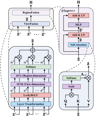
Figure 3: Dual-feature attentive fusion and its components. (1) DAFusion (upper left); (2) ViewFusion (lower left); (3) RegionFusion (right).

View-aware attentive fusion. ViewFusion leverages the attention mechanism to learn fusion weights that indicate the relative importance of the views to aggregate the view-based embeddings {$\mathbf{Z}^{1},\mathbf{Z}^{2},...,\mathbf{Z}^{v}\}$. It first computes correlation scores between different views by adopting a simplified self-attention [36] as follows:

$$a^{jk}_{i}=\mathrm{LeakyReLU}\big{(}\mathbf{a}^{\intercal}(\mathbf{W}_{F}\mathbf{z}^{j}_{i}||\mathbf{W}_{F}\mathbf{z}^{k}_{i})\big{)},$$ (1)

where $a^{jk}_{i}$ is the correlation score between the $j$-th and the $k$-th views of region $r_{i}$, $\mathbf{a}\in\mathbb{R}^{2d^{\prime}}$ and $\mathbf{W}_{F}\in\mathbb{R}^{d^{\prime}\times d}$ are learnable parameters (Linear Transformation in Fig. 3), $d^{\prime}$ is the dimensionality of the latent representation ($d^{\prime}=64$ in the experiments), ‘$||$’ denotes concatenation and LeakyReLU is an activation function.

Then, we aggregate the correlation scores along the views and the regions to obtain an overall weight for each view, and then we apply a Softmax function to obtain the normalized fuse weight $\alpha^{j}$ ($j\in[1,v]$) of each view.

$$\alpha^{j}=\mathrm{Softmax}(\frac{1}{n}\sum^{n}_{i=1}\sum^{v}_{k=1}a_{i}^{jk}),$$ (2)

We use the fusion weights to fuse the view-based embeddings into a single embedding matrix, denoted as $\widetilde{\mathbf{Z}}\in\mathbb{R}^{n\times d}$:

$$\widetilde{\mathbf{Z}}=\sum_{j=1}^{v}\alpha^{j}\cdot\mathbf{Z}^{j}$$ (3)

Region-aware attentive fusion. RegionFusion further applies self-attention [43] on the embeddings $\widetilde{\mathbf{Z}}$ learned by ViewFusion, to encode the higher order correlations among the learned region embeddings.

As Fig. 3 shows, the embeddings $\widetilde{\mathbf{Z}}$ are first fed into a self-attention module, which applies linear transformations to $\widetilde{\mathbf{Z}}$ to form three projected matrices in latent spaces, i.e., a query matrix $\mathbf{Q}\in\mathbb{R}^{n\times d}=\mathbf{W}_{Q}\widetilde{\mathbf{Z}}$, a key matrix $\mathbf{K}\in\mathbb{R}^{n\times d}=\mathbf{W}_{K}\widetilde{\mathbf{Z}}$, and a value matrix $\mathbf{V}\in\mathbb{R}^{n\times d}=\mathbf{W}_{V}\widetilde{\mathbf{Z}}$. Here, $\mathbf{W}_{Q}$, $\mathbf{W}_{K}$, and $\mathbf{W}_{V}$ are learned parameter matrices of the linear transformations and are all in $\mathbb{R}^{d\times d}$. Multi-head attention [43] is applied here to enhance the model learning capacity, while its details are omitted as it is a direct adoption.

Next, we compute attention coefficients between regions:

$$\mathbf{A}_{rf}=\mathrm{Softmax}\big{(}\frac{\mathbf{Q}\cdot{\mathbf{K}}^{\intercal}}{\sqrt{d}}\big{)},$$ (4)

where $\sqrt{d}$ is a scaling factor and $\mathbf{A}_{rf}\in\mathbf{R}^{n\times n}$ is a coefficient matrix that records the correlation between every two regions.

After that, we compute hidden representations of the regions based on the attention coefficients $\mathbf{A}_{rf}$:

$$\hat{\mathbf{Z}}=\mathbf{A}_{rf}\cdot\mathbf{V}.$$ (5)

The output of the self-attention module $\hat{\mathbf{Z}}$ is added with the input embeddings $\widetilde{\mathbf{Z}}$ (through a residual connection) and then goes through a layer normalization (LN) with dropout (to alleviate issues of exploding and vanishing gradients). Subsequently, a multi-layer perceptron (MLP) and another layer normalization (again with a residual connection) are applied to enhance the model learning capacity. These steps can be summarized as follows:

$$\hat{\mathbf{Z}}^{\prime}=\mathrm{LayerNorm}(\widetilde{\mathbf{Z}}+\mathrm{Dropout}(\hat{\mathbf{Z}})),$$ (6)

$${\mathbf{H}}=\mathrm{LayerNorm}(\hat{\mathbf{Z}}^{\prime}+\mathrm{Dropout}(\mathrm{MLP}(\hat{\mathbf{Z}}^{\prime}))).$$ (7)

Here, $\hat{\mathbf{Z}}^{\prime}$ is the output of the first layer normalization, and $\mathbf{H}$ is the output region embeddings.

We stack multiple layers of the structure above, and the output of the final layer is our learned region embeddings $\mathbf{H}$.

IV-C Model Training

We present a multi-task learning objective $\mathcal{L}$ with $v$ sub-objective functions $\mathcal{L}^{1},\mathcal{L}^{2},\ldots,\mathcal{L}^{v}$ to guide our model HAFusion to learn generic and robust region representations:

$$\mathcal{L}=\mathcal{L}^{1}+\mathcal{L}^{2}+\ldots+\mathcal{L}^{v}$$ (8)

Here, each sub-objective function $\mathcal{L}^{j}$ ($j\in[1,v]$) focuses on learning from an input feature.

Given that there are no external supervision signals (e.g., region class labels), we use the similarity between the regions as computed by their input feature vectors to guide model training. To compute $\mathcal{L}^{j}$, we use an MLP (i.e., a linear layer and a ReLU activation function) to map the region embedding matrix $(\mathbf{H})$ to an input-feature-oriented region embedding matrix $(\mathbf{H})^{j}$, i.e., $\mathbf{H}^{j}=\mathrm{MLP}(\mathbf{H})$. Then,

$$\mathcal{L}^{j}=\frac{1}{n}\frac{1}{n}\sum_{i=1}^{n}\sum_{k=1}^{n}\Big{|}\mathrm{cos}(\mathbf{x}^{j}_{i},\mathbf{x}^{j}_{k})-{\mathbf{h}^{j}_{i}}\cdot\mathbf{h}^{j}_{k}\Big{|}$$ (9)

Here, $\mathbf{x}^{j}_{i}$ and $\mathbf{x}^{j}_{k}$ are feature vectors of regions $r_{i}$ and $r_{k}$ of the $j$-th input feature, and $\mathrm{cos}(\cdot)$ computes their cosine similarity. Vectors $\mathbf{h}^{j}_{i}$ and $\mathbf{h}^{j}_{k}$ from $\mathbf{H}^{j}$ are the learned embeddings of $r_{i}$ and $r_{k}$ mapped towards the $j$-th feature, and their dot product represents the region similarity in the embedding space. The intuition is that the learned embeddings should reflect the region similarity as entailed by the input features. We note that the cosine similarity of $\mathbf{h}^{j}_{i}$ and $\mathbf{h}^{j}_{k}$ can be used in Equation 9 instead of the dot product. Empirically, we find that both approaches produce embeddings that yield very similar accuracy in downstream tasks, while using the cosine similarity takes more time in embedding learning. Thus, we have used the dot product instead.

The loss function above is generic and can be applied to input features without requiring further domain knowledge. We use it for the POI and land use features. For the human mobility features, they entail both the source and the destination distribution patterns of human mobility. While the sub-objective function above also works, we follow previous studies [10, 14, 22] and use a KL-divergence based sub-objective function described below.

Mobility distribution loss. Using the human mobility feature matrix $\mathbf{M}$ (cf. Section III). We compute two transition probabilities for movements from region $r_{i}$ to region $r_{k}$:

$$\begin{aligned} p_{s}(r_{k}|r_{i})=\frac{m_{i,k}}{\sum^{n}_{l=1}m_{i,l}},\end{aligned}\quad\quad\begin{aligned} p_{d}(r_{k}|r_{i})=\frac{m_{i,k}}{\sum^{n}_{l=1}m_{l,k}}\end{aligned}$$ (10)

Here, $p_{s}(\cdot)$ denotes how likely people move to region $r_{k}$ when they move out from region $r_{i}$, and $p_{d}(\cdot)$ denotes how likely people come from $r_{i}$ when they move into $r_{k}$.

To enable computing the KL-divergence loss, we need such probability values from the learned embeddings. We map $\mathbf{H}$ into a source feature-oriented matrix $\mathbf{H}^{S}$ and a destination feature-oriented $\mathbf{H}^{D}$ (each with an MLP like above). We compute two transition probabilities with these matrices:

$$\hat{p_{s}}(r_{k}|r_{i})=\frac{\exp(\mathbf{h}^{S}_{i}\cdot\mathbf{h}^{D}_{k})}{\sum^{n}_{l=1}\exp(\mathbf{h}^{S}_{i}\cdot\mathbf{h}^{D}_{l})}$$ (11)

$$\hat{p_{d}}(r_{k}|r_{i})=\frac{\exp(\mathbf{h}^{S}_{i}\cdot\mathbf{h}^{D}_{k})}{\sum^{n}_{l=1}\exp(\mathbf{h}^{S}_{l}\cdot\mathbf{h}^{D}_{k})}$$ (12)

Here, $\mathbf{h}^{S}_{i}\in\mathbf{H}^{S}$ and $\mathbf{h}^{D}_{k}\in\mathbf{H}^{D}$ correspond to regions $r_{i}$ and $r_{k}$, respectively. The KL divergence loss is then computed:

$$\mathcal{L}^{M}=\sum_{i=1}^{n}\sum_{k=1}^{n}\big{(} -p_{s}(r_{k}|r_{i})\log(\hat{p_{s}}(r_{k}|r_{i}))$$ (13)

$$-p_{d}(r_{k}|r_{i})\log(\hat{p_{d}}(r_{k}|r_{i}))\,\big{)}.$$

V Hybrid Attentive Feature Learning

Motivated by the strong learning performance of our attention-based fusion module, we further propose an attention-based embedding learning module for the view-based embedding learning process, i.e., the hybrid attentive feature learning (HALearning) module, as mentioned in Section IV-A.

HALearning consists of an intra-view attentive feature learning (IntraAFL) module and an inter-view attentive feature learning (InterAFL) module to generate view-based region embeddings. IntraAFL encodes region correlation information entailed in the input features of each single view, while InterAFL further captures region correlation across views.

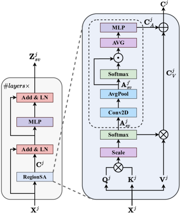
Figure 4: Intra-view attentive feature learning (IntraAFL).

Intra-view attentive feature learning. Fig. 4 shows the structure of the IntraAFL module, which is also based on the Transformer encoder [43] structure like the RegionFusion  module described earlier, except that its input is a view matrix $\mathbf{X}^{j}$ and its output is an intermediate region embedding matrix, denoted by $\mathbf{Z}^{j}_{sv}$ (“$sv$” refers to “single view”).

We do not repeat the full computation steps of IntraAFL. Instead, we focus on its RegionSA module (right sub-figure in Fig. 4), which is our new design for learning both region correlations and region embeddings within each view.

RegionSA adapts the vanilla multi-head self-attention by incorporating a simple yet effective module (inside the dashed rectangle in Fig. 4). It takes as input the region features of one view, $\mathbf{X}^{j}$, and computes the attention coefficient scores between the regions, denoted by $\mathbf{A}^{j}_{sv}$, and the latent region representations, denoted by $\mathbf{C}^{j}_{V}$. The calculations are similar to Equations 4 and 5 except that the inputs to the equations are different. We hence do not repeat the equations again.

Next, we aim to combine the intermediate view-based region embeddings $\mathbf{C}^{j}_{V}$ and the coefficient score matrix $\mathbf{A}^{j}_{sv}$, such that the region embeddings further encode the region correlation information. We observe that it is sub-optimal to directly concatenate the two matrices. This is because the coefficient score matrix $\mathbf{A}^{j}_{sv}$ is obtained by computing the correlation between every two regions. It does not capture the correlations among multiple regions, e.g., the feature of a region may be impacted by multiple regions jointly.

To address this issue, we introduce a lightweight module (inside the dashed rectangle in Fig. 4) applied on $\mathbf{A}^{j}_{sv}$ to learn multi-region correlations. We first employ a 2-dimensional convolution layer and an average pooling layer, denoted as Conv2D and AvgPool, to compute a correlation matrix (in $\mathbb{R}^{c\times n\times n}$) that learns the higher-order region correlations (entailed in convolution operation), where $c$ is a hyper-parameter ($c=64$ in our experiments). Let the resulting matrix be ${\mathbf{A}^{j^{\prime}}_{sv}}$. We compute the element-wise product between ${\mathbf{A}^{j^{\prime}}_{sv}}$ and its normalized version (obtained by a Softmax layer). Finally, we average the resulting matrix and project the matrix to $\mathbb{R}^{n\times d}$ with an MLP, such that it can be added with $\mathbf{C}^{j}_{V}$. The steps above are summarized as follows:

$${\mathbf{A}^{j^{\prime}}_{sv}}=\mathrm{AvgPool}(\mathrm{Conv2D}({\mathbf{A}^{j}_{sv}})),$$ (14)

$$\mathbf{C}^{j}_{A}=\mathrm{MLP}(\mathrm{AVG}({\mathbf{A}^{j^{\prime}}_{sv}}\odot\mathrm{Softmax}({\mathbf{A}^{j^{\prime}}_{sv}}))).$$ (15)

Then, we encode the region correlation information into the region embeddings as the output of RegionSA, denoted as $\mathbf{C}^{j}$:

$$\mathbf{C}^{j}=\mathbf{C}^{j}_{V}+\mathbf{C}^{j}_{A}.$$ (16)

Matrix $\mathbf{C}^{j}$ will go through the rest of the computation steps of IntraAFL as shown in the left sub-figure of Fig. 4 (which resemble Equations 6 and 7) to produce the output embeddings of the module, $\mathbf{Z}^{j}_{sv}$. Overall, from the $v$ input views, we will obtain $v$ embedding matrices, $\mathbf{Z}_{sv}^{1},\mathbf{Z}_{sv}^{2},\ldots,\mathbf{Z}_{sv}^{v}$. We call these matrices the intra-view attentive region embedding matrices.

Inter-view attentive feature learning. Next, we present InterAFL to learn correlations between regions across views. Note that we consider the correlations between all regions across all views, instead of only the same region from different views as done in existing works [10, 15, 14, 22].

A naive method is to apply self-attention over $\mathbf{Z}_{sv}$, like RegionFusion does, to compute correlation coefficients between all pairs of regions from the same and different views. This approach, however, is computationally expensive, as $\mathbf{Z}_{sv}^{1},\mathbf{Z}_{sv}^{2},\ldots,\mathbf{Z}_{sv}^{v}$ together form a large matrix in $\mathbb{R}^{n\times v\times d}$, and it introduces unnecessary noise signals – many regions far away from each other are unlikely to be correlated.

To avoid these issues, we introduce a learnable memory unit [44] to help effectively and efficiently learn the correlations among the regions across views. Fig. 5 shows the structure of InterAFL. The memory unit stores a list of $d^{m}$ ($d^{m}=144$ in the experiments) learned representative embeddings in the latent region embedding space (which can be thought of as the cluster centers of the region embeddings). We learn the correlations between each region and the representative embeddings in the memory unit to implicitly learn the correlation between the region and the rest of the regions, since the memory unit serves as a summary of the latent embedding space. As there are limited embeddings in the memory unit, the learning process can be done efficiently.

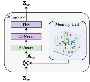
Figure 5: Inter-view attentive feature learning (InterAFL).

InterAFL reads the embedding matrices $\{\mathbf{Z}_{sv}^{j}\}_{j=1}^{v}$ from IntraAFL and concatenates them into one large matrix $\mathbf{Z}_{sv}\in\mathbb{R}^{n\times v\times d}$ for ease of process. It computes the correlation coefficients between all regions in $\mathbf{Z}_{sv}$ and the memory unit:

$$\mathbf{A}_{cv}=\mathrm{FFN}(\mathbf{Z}_{sv})$$ (17)

where $\mathbf{A}_{cv}$ denotes inter-view region correlation coefficients between regions. $\mathrm{FFN}(\cdot)$ denotes a feedforward neural network, where the weight matrix is in $\mathbb{R}^{d\times d^{m}}$. The $d^{m}$ vectors in this weight matrix are considered as the representative embeddings (of $d$ dimensions). They can be seen as $d^{m}$ randomly sampled cluster centers in the latent region embedding space.

Then, the inter-view region correlation coefficients are fed into two normalization layers (i.e., a Softmax layer and an L1-Norm layer) and another FFN to produce embeddings $\mathbf{Z}_{cv}$ embedded with cross-view region correlation coefficients:

$$\mathbf{Z}_{cv}=\mathrm{FFN}(\mathrm{L1{\text{-}}{Norm}}(\mathrm{Softmax(\mathbf{A}_{cv})}))$$ (18)

where the weight matrix of the FFN is in $\mathbb{R}^{d^{m}\times d}$. Here, the Softmax layer is applied on the second dimension (i.e., the view dimension), and the L1-Norm layer is applied on the third dimension (i.e., the embedding dimension). We repeat the computations above for multiple layers to enhance the model learning capacity. The final $\mathbf{Z}_{cv}$ output of InterAFL can be decomposed into a list of sub-matrices by the second dimension (the views), i.e., $\mathbf{Z}_{cv}^{1},\mathbf{Z}_{cv}^{2},...,\mathbf{Z}_{cv}^{v}$, where each sub-matrix is in $\mathbb{R}^{n\times d}$. We call these matrices the inter-view attentive region embedding matrices.

Finally, we adaptively combine the intra-view attentive region embedding matrices $\{\mathbf{Z}_{sv}^{j}\}$ and the inter-view attentive region embedding matrices $\{\mathbf{Z}_{cv}^{j}\}$ with a learnable weight $\beta\in[0,1]$, to form the view-based region embeddings $\{\mathbf{Z}^{j}\}$:

$${\mathbf{Z}^{j}}=\beta{\mathbf{Z}_{sv}^{j}}+(1-\beta){\mathbf{Z}_{cv}^{j}}$$ (19)

VI EXPERIMENTS

We perform an empirical study to verify: (Q1) the accuracy of our proposed model HAFusion on three downstream tasks as compared with the state-of-the-art (SOTA) methods, (Q2) the general applicability of our proposed dual-feature attentive fusion technique when incorporated into existing multi-view region representation learning models, (Q3) the effectiveness of our model components, and (Q4) the impact of our model hyper-parameters.

TABLE II: Dataset Statistics

3	NYC [40]	CHI [41]	SF [42]
#regions	180	77	175
#POIs	24,496	57,891	28,578
#POI categories	26	26	26
#land use categories	11	12	23
#taxi trips	10,953,879	3,381,807	357,749
(data collection time)	06/2015 - 07/2015	01/2021 - 01/2022	05/2008 - 06/2008
#crime records	35,335	18,200	48,489
(data collection time)	unknown	12/2022 - 12/2022	01/2022 - 12/2022
#check-ins	106,902	167,232	87,750
(data collection time)	04/2012 - 09/2013	04/2012 - 09/2013	04/2012 - 09/2013
#service calls	516,187	24,350	34,385
(data collection time)	01/2023 - 03/2023	12/2022 - 12/2022	01/2022 - 12/2022
3

VI-A Experimental Settings

Dataset. The experiments are conducted using real-world data from cities: New York City (NYC) [40], Chicago (CHI) [41], and San Francisco (SF) [42]. Previous works [10, 22, 14] only used NYC, while CHI and SF are used for the first time in our study, to show the general applicability of our model across different datasets. We plan to release the datasets and our source code upon paper publication.

Table II summarizes the datasets. For each city, we have:

(1) region boundary of each region;

(2) taxi trip records including the pickup and drop-off points of each trip – we use the numbers of trips from a region to the others as the mobility feature vector of the region;

(3) POIs in each region (from OpenStreetMap [39]), along with their category labels as described in Section III;

(4)) zones in each region, along with their land use category labels as described in Section III – there are 11, 12, and 13 categories for NYC, CHI, and SF, respectively;

(5) crime, check-in (from a Foursquare dataset [45]), and service call records, each with a location and a time – we count the number of these records in each region, respectively, and predict the counts using the region embeddings learned from the features above, following previous works [10, 22, 14].

Prediction model. We use three downstream tasks for model evaluation, i.e., crime, check-in, and service call count prediction, which are regression tasks. We implement a Lasso regression model (model parameter $\alpha=1$) for each prediction task, following previous works [22, 14, 10].

Evaluation metrics. We use three classic evaluation metrics for regression tasks: Mean Absolute Error (MAE), Root Mean Square (RMSE), and Coefficient of Determination ($\boldsymbol{R^{2}}$).

Competitors. We compare with the following models, including the SOTA models RegionDCL [26] and HREP [14]:

(1) MVURE [10] leverages both the intra-region (POI and check-in features) and inter-region features (human mobility features) to construct multi-view graphs, which is followed by multi-view fusion to learn region embeddings.

(2) MGFN [22] leverages human mobility features to construct mobility pattern graphs by clustering mobility graphs based on their spatio-temporal distances. Afterwards, it performs inter-view and intra-view messages passing on the mobility pattern graphs to generate region embeddings.

(3) RegionDCL [26] leverages building footprints from OpenStreetMap and uses contrastive learning at both the building-group and region levels to learn building-group embeddings. Afterwards, it aggregates all building-group embeddings in a region to generate region embeddings.

(4) HREP [14] leverages human mobility, POI, and geographic neighbor features to generate region embeddings. Subsequently, it integrates task-based learnable prompt embeddings with the pre-trained region embeddings to customize the embeddings for different downstream tasks.

TABLE III: Overall Prediction Accuracy Results (‘$\downarrow$’ indicates that smaller values are preferred, and ‘$\uparrow$’ indicates that large values are preferred. The best results are in boldface, and the second best results are underlined. Same for the tables below.)

Taks 1: Check-in	New York City			Chicago			San Francisco
	MAE $\downarrow$	RMSE $\downarrow$	$R^{2}\uparrow$	MAE $\downarrow$	RMSE $\downarrow$	$R^{2}\uparrow$	MAE $\downarrow$	RMSE $\downarrow$	$R^{2}\uparrow$
MVURE [10]	306.7 $\pm$ 8.20	499.6 $\pm$ 12.9	0.627 $\pm$ 0.019	1721 $\pm$   68	3339 $\pm$ 147	0.618 $\pm$ 0.033	346.8 $\pm$ 8.7	659.3 $\pm$ 15.7	0.562 $\pm$ 0.021
MGFN [22]	292.6 $\pm$ 17.1	451.8 $\pm$ 28.1	0.690 $\pm$ 0.040	1281 $\pm$   41	2276 $\pm$   86	0.817 $\pm$ 0.011	310.8 $\pm$ 9.1	542.1 $\pm$ 17.6	0.708 $\pm$ 0.010
RegionDCL [26]	371.2 $\pm$ 10.3	495.5 $\pm$ 15.9	0.471 $\pm$ 0.023	2427 $\pm$ 123	4184 $\pm$ 136	0.402 $\pm$ 0.042	398.8 $\pm$ 9.9	748.1 $\pm$ 17.8	0.437 $\pm$ 0.024
HREP [14]	276.3 $\pm$ 11.7	448.2 $\pm$ 17.1	0.703 $\pm$ 0.021	1702 $\pm$   79	3301 $\pm$ 101	0.628 $\pm$ 0.023	330.9 $\pm$ 9.3	606.7 $\pm$ 25.8	0.629 $\pm$ 0.032
HAFusion	202.8 $\pm$ 7.2	322.8 $\pm$ 12.6	0.844 $\pm$ 0.012	929 $\pm$   62	1947 $\pm$   75	0.870 $\pm$ 0.010	233.1 $\pm$ 9.5	429.6 $\pm$ 28.1	0.813 $\pm$ 0.024
Improvement	26.6%	28.0%	20.6%	27.4%	14.5%	6.5%	25%	20.7%	14.8%
Task 2: Crime	New York City			Chicago			San Francisco
	MAE $\downarrow$	RMSE $\downarrow$	$R^{2}\uparrow$	MAE $\downarrow$	RMSE $\downarrow$	$R^{2}\uparrow$	MAE $\downarrow$	RMSE $\downarrow$	$R^{2}\uparrow$
MVURE [10]	67.9 $\pm$ 1.1	93.8 $\pm$ 1.9	0.591 $\pm$ 0.016	100.4 $\pm$ 6.6	129.2 $\pm$ 7.3	0.461 $\pm$ 0.062	130.3 $\pm$ 1.7	201.7 $\pm$ 3.2	0.594 $\pm$ 0.013
MGFN [22]	70.2 $\pm$ 2.3	89.6 $\pm$ 2.5	0.630 $\pm$ 0.020	107.4 $\pm$ 5.4	137.9 $\pm$ 5.2	0.386 $\pm$ 0.047	128.4 $\pm$ 3.3	199.9 $\pm$ 4.3	0.601 $\pm$ 0.017
RegionDCL [26]	98.7 $\pm$ 3.1	127.9 $\pm$ 5.2	0.251 $\pm$ 0.026	121.7 $\pm$ 4.8	159.6 $\pm$ 6.3	0.179 $\pm$ 0.053	156.3 $\pm$ 2.1	242.3 $\pm$ 4.6	0.413 $\pm$ 0.021
HREP [14]	62.8 $\pm$ 2.1	83.1 $\pm$ 2.3	0.680 $\pm$ 0.014	88.3 $\pm$ 6.4	114.4 $\pm$ 5.5	0.578 $\pm$ 0.041	124.4 $\pm$ 2.3	196.9 $\pm$ 3.9	0.612 $\pm$ 0.014
HAFusion	56.1 $\pm$ 1.3	76.1 $\pm$ 2.2	0.734 $\pm$ 0.015	77.8 $\pm$ 3.6	107.1 $\pm$ 5.4	0.631 $\pm$ 0.036	101.5 $\pm$ 3.3	178.4 $\pm$ 3.6	0.682 $\pm$ 0.013
Improvement	10.8%	8.4%	7.8%	11.9%	6.4%	9.2%	18.4%	9.4%	11.4%
Task 3: Service call	New York City			Chicago			San Francisco
	MAE $\downarrow$	RMSE $\downarrow$	$R^{2}\uparrow$	MAE $\downarrow$	RMSE $\downarrow$	$R^{2}\uparrow$	MAE $\downarrow$	RMSE $\downarrow$	$R^{2}\uparrow$
MVURE [10]	1428 $\pm$ 33	2180 $\pm$   46	0.367 $\pm$ 0.027	190.3 $\pm$   9.8	266.9 $\pm$ 12.1	0.441 $\pm$ 0.050	102.1 $\pm$ 4.8	164.7 $\pm$ 2.7	0.479 $\pm$ 0.017
MGFN [22]	1554 $\pm$ 81	2286 $\pm$ 115	0.303 $\pm$ 0.069	208.2 $\pm$ 11.3	293.4 $\pm$ 16.6	0.329 $\pm$ 0.077	102.8 $\pm$ 2.2	166.3 $\pm$ 2.5	0.468 $\pm$ 0.021
RegionDCL [26]	1783 $\pm$ 21	2597 $\pm$   38	0.103 $\pm$ 0.026	195.7 $\pm$   7.6	272.1 $\pm$ 10.1	0.445 $\pm$ 0.041	116.6 $\pm$ 2.3	196.7 $\pm$ 3.2	0.256 $\pm$ 0.024
HREP [14]	1430 $\pm$ 29	2286 $\pm$   34	0.398 $\pm$ 0.021	185.7 $\pm$   6.1	262.2 $\pm$ 10.8	0.468 $\pm$ 0.022	103.4 $\pm$ 3.2	167.4 $\pm$ 4.6	0.461 $\pm$ 0.029
HAFusion	1273 $\pm$ 20	1951 $\pm$   27	0.493 $\pm$ 0.014	159.3 $\pm$ 13.9	222.0 $\pm$ 18.9	0.613 $\pm$ 0.067	81.5 $\pm$ 2.5	142.1 $\pm$ 3.2	0.612 $\pm$ 0.018
Improvement	10.9%	8.3%	23.9%	14.2%	15.3%	31.0%	20.2%	13.7%	27.8%

Hyperparameter settings. For the competitor models, we use parameter settings recommended in their papers as much as possible. Special settings have been made on CHI, to prevent model overfitting on this dataset which has fewer regions. For MGFN, we employ a 1-layer (instead of the default 3-layer) mobility pattern joint learning module on CHI. For MVURE and HREP, we reduce the number of layers in their GNN modules from 3 to 2 on CHI. RegionDCL does not need a special setting on CHI because the training process is determined by the number of buildings and building groups, rather than the number of regions.

For our model HAFusion, the number of layers in the IntraAFL module is 3 for NYC and SF and 1 for CHI, respectively. In the InterAFL module, the number of layers is 3 for NYC and 2 for CHI and SF, respectively. The number of layers in the RegionFusion module is 3 for all three datasets. These parameter values are set by a grid search. We train our model for 2,500 epochs in full batches, using Adam optimization with a learning rate of 0.0005.

The region embedding dimensionality $d$ is set as 144 for HAFusion following an SOTA model HREP [14], and 96, 96, and 64 for MVURE, MGFN, and RegionDCL, respectively, as suggested by their original papers.

VI-B Overall Results

We evaluate the quality of the learned region embeddings through using them in three downstream prediction tasks. We first learn region embeddings using each model on data from each city, respectively. We subsequently feed the learned region embeddings into a Lasso regression model for each prediction task, employing ten-fold cross-validation (because the number of regions in each dataset is relatively small), and report in Table III the average prediction accuracy results.

VI-B1 Task 1: Check-in Count Prediction

Predicting check-in counts for regions can provide guidance for urban planning, business decision-making, and public safety management (e.g., movement tracking [46, 47]), based on people’s locations and interests.

We make the following observations from Table III (Task 1):

(1) Our model HAFusion outperforms all competitors across all datasets with up to 28% improvement in RMSE. Our model not only considers various types of features of each region but also learns the correlation among the features of different regions both within a single view and across multiple views, which enables the learned embeddings to capture the feature patterns to a full extent. Simultaneously, we effectively fuse the patterns to extract their joint impact, leading to highly effective embeddings for region-based prediction tasks.

(2) MGFN, which only considers one input feature (i.e., human mobility), outperforms (up to 20% in terms of $R^{2}$) the baseline methods MVURE and HREP that use human mobility, POI, geographic neighbor, and check-in features, on CHI and SF datasets, while it performs worse on NYC. There are three main reasons: (i) human mobility is intrinsically linked to the check-in count of each region. (ii) MGFN explores the complex mobility patterns from the human mobility data, allowing it to learn the relationships among regions from such patterns. (iii) the human mobility data of NYC is noisy, which negatively impacts the learning effectiveness of MGFN. In this case, the limitations of relying on a single data feature become evident, emphasizing the necessity to gather information from multiple data sources as done in our model HAFusion.

(3) HREP outperforms MVURE across all three datasets, as it introduces a relational embedding to capture different correlations among regions, which helps encode the importance of correlations among regions into the region embeddings. It also incorporates prompt learning to add task-specific prompt embeddings for different downstream task.

(4) RegionDCL performs the worst, even though it is one of the SOTA models. It only utilizes building footprints to learn region embeddings (its original targeted downstream tasks are population and land use predictions [26]), which do not exhibit a strong correlation with the check-in counts. Furthermore, distinguishing the functionality of regions by buildings can be challenging in cities such as NYC, where buildings predominantly take on a rectangular shape, irrespective of whether they are situated in industrial or residential areas. In addition, RegionDCL is based on contrastive learning, which is biased to generate similar embeddings for regions nearby.

VI-B2 Task 2: Crime Prediction

Predicting crime counts in different regions is a valuable tool for law enforcement and community safety, as it allows for a more proactive and strategic approach to crime prevention and reduction.

Table III (Task 2) presents model performance for such a task.

Our model HAFusion again outperforms the best competitor model HREP across all datasets (7.8% on NYC, 9.2% on CHI, and 11.4% on SF in $R^{2}$), for our more effective multi-view fusion techniques to capture inter-region relationships.

The baseline models MVURE and HREP that take multiple types of input features are now also better than those taking only a single type of feature, i.e., MGFN and RegionDCL. Crime counts are impacted by multiple factors. Regions with high crime counts typically have a high level of human mobility, many entertainment venues such as bars and clubs, and are proximity to public transportation. These factors cannot be reflected by only a single type of region features.

VI-B3 Task 3: Service Call Prediction

Predicting service calls in each region is a valuable tool for service providers, allowing proactive optimization of facility and service deployments, which helps improve the urban living experience.

As Table III shows, our model HAFusion achieves consistent and substantial improvements over all competitors, with an advantage over the best baseline results by 23.9% on NYC, 31% on CHI, and 27.8% on SF in terms of $R^{2}$, respectively, further confirming the robustness of the embeddings learned by HAFusion for urban prediction tasks.

Like in the crime count prediction task, the baseline models MVURE and HREP which consider multiple types of input features, once again outperform MGFN and RegionDCL.

Model performance on NYC is, in general, lower than that on CHI and SF. This is because NYC contains about 400 categories of service calls, including noise complaints, graffiti cleanup, etc., while SF and CHI only have 67 and 104, respectively. It is more challenging to generate region embeddings that correlate to all these different types of calls.

TABLE IV: Embedding Learning and Downstream Task Running Times (seconds)

3	Embedding Learning			Downstream Task
	NYC	CHI	SF	NYC	CHI	SF
MVURE	557	153	518	0.016	0.049	0.028
MGFN	1,452	460	1,388	0.017	0.054	0.032
RegionDCL	2,004	17,435	5,748	0.014	0.051	0.026
HREP	302	136	267	171	325	152
HAFusion	934	346	856	0.019	0.062	0.037
3

TABLE V: Prediction Accuracy Results When Powering Existing Models with Our DualAFM Module (NYC)

3 New York City	Check-in Prediction			Crime Prediction			Service Call Prediction
	MAE $\downarrow$	RMSE $\downarrow$	$R^{2}\uparrow$	MAE $\downarrow$	RMSE $\downarrow$	$R^{2}\uparrow$	MAE $\downarrow$	RMSE $\downarrow$	$R^{2}\uparrow$
MGFN	292.6 $\pm$ 17.1	451.8 $\pm$ 28.1	0.690 $\pm$ 0.040	70.2 $\pm$ 2.3	89.6 $\pm$ 2.5	0.630 $\pm$ 0.020	1553.8 $\pm$ 80	2286 $\pm$ 115	0.303 $\pm$ 0.069
MGFN-DualAFM	222.0 $\pm$   5.7	363.6 $\pm$   8.5	0.802 $\pm$ 0.009	59.8 $\pm$ 1.2	81.1 $\pm$ 2.4	0.699 $\pm$ 0.018	1375.7 $\pm$ 16	2101 $\pm$   29	0.412 $\pm$ 0.016
Improvement	24.2%	19.5%	16.2%	14.8%	9.5%	11.0%	11.5%	8.1%	36.0%
MVURE	306.7 $\pm$ 8.2	499.6 $\pm$ 12.9	0.627 $\pm$ 0.019	67.9 $\pm$ 1.1	93.8 $\pm$ 1.9	0.591 $\pm$ 0.016	1428 $\pm$ 33	2180 $\pm$ 46	0.367 $\pm$ 0.027
MVURE-DualAFM	275.8 $\pm$ 5.9	438.5 $\pm$ 14.4	0.712 $\pm$ 0.018	62.6 $\pm$ 1.5	85.9 $\pm$ 1.9	0.663 $\pm$ 0.015	1317 $\pm$ 16	2049 $\pm$ 33	0.441 $\pm$ 0.018
Improvement	10.1%	12.2%	13.6%	7.8%	8.4%	12.4%	7.8%	6.0%	20.2%
HREF	276.3 $\pm$ 11.7	448.2 $\pm$ 16.9	0.703 $\pm$ 0.022	62.8 $\pm$ 2.1	83.1 $\pm$ 2.3	0.681 $\pm$ 0.014	1430 $\pm$ 29	2127 $\pm$ 34	0.398 $\pm$ 0.019
HREF-DualAFM	224.6 $\pm$   8.5	360.0 $\pm$ 10.3	0.806 $\pm$ 0.011	59.2 $\pm$ 1.6	78.6 $\pm$ 1.3	0.717 $\pm$ 0.011	1325 $\pm$ 19	2031 $\pm$ 29	0.451 $\pm$ 0.015
Improvement	18.7%	19.7%	15.1%	5.7%	5.4%	5.3%	7.3%	4.5%	13.3%

Model running time. Table IV reports the embedding learning and downstream task running times (including regression model learning and inference, and they have the same input and output size irrespective to the exact downstream tasks). All models are trained and tested on a computer running Windows 10 with a 16-core Intel i7 2.6 GHz CPU and 16 GB memory (same for the rest of the experiments).

HAFusion takes extra time to learn the embeddings because of its extra attention computation and fusion steps. However, we see that its embedding learning time is still on the same order of magnitude as that of the fastest model HERP, which on the other hand is very slow at testing with the downstream tasks, because it requires extra task-based prompt embedding learning for each downstream task. Also, HAFusion can be trained on a CPU in just 15 minutes, which makes it highly practical in terms of the training cost.

MVURE and HREP simply aggregate region embeddings from all views, which are faster to train, but this efficiency comes at the cost of significantly higher prediction errors with their learned embeddings, as shown above.

All models share the same prediction model for the downstream tasks, and hence their downstream task running times are very similar (except for HREP). The slight difference in the running times is due to the difference in the embedding dimensionality. HREP is much slower because it requires a prompt embedding learning step for each downstream task.

VI-C Applicability of Dual-feature Attentive Fusion

To show the general applicability of our dual-feature attentive fusion module (DAFusion), we integrate it with the three baseline models that compute multiple views and require an embedding fusion, i.e., MVURE, MGFN, and HREP. We denote the resulting models as MVURE-DAFusion, MGFN-DAFusion, and HREP-DAFusion, respectively.

We run experiments with the three datasets and three downstream tasks on these new model variants, with 10-fold cross-validation as done above. We show the results on NYC in Table V for conciseness, as the results on the other two datasets have a similar comparative pattern. We see that DAFusion can also enhance the effectiveness of learning region embeddings for the existing multi-view based models. Compared to the vanilla models, the variants powered by DAFusion achieve significant improvements, i.e., up to 16.2%, 12.4%, and 36% in terms ${R^{2}}$, across the three downstream prediction tasks. These results confirm the effectiveness and wide applicability of our DAFusion module. The improvement on MGFN, in particular, indicates that DAFusion can also better integrate information from multiple graphs even when the graphs are constructed using a single type of input feature.

By further comparing the results in Tables III and V, we note that our HAFusion still outperforms the baseline models even when they are powered by DAFusion, which confirms the contribution of our hybrid attentive feature learning module to the overall model accuracy. We further verify this with an ablation study next.

VI-D Ablation Study

We use the following model variants to study the effectiveness of our model components:

(1) HAFusion-w/o-D$+$: We replace DAFusion with a simple element-wise sum of embeddings from different views.

(2) HAFusion-w/o-D$\|$: We replace DAFusion with a simple concatenation of the embeddings from different views, followed by an MLP layer to reduce the dimensionality.

(3) HAFusion-w/o-C: We replace InterAFL with the vanilla self-attention.

(4) HAFusion-w/o-S: We replace IntraAFL with the vanilla self-attention.

TABLE VI: Ablation Study Results (NYC)

3  Prediction Task	Check-in	Crime	Service Call
	$R^{2}\uparrow$	$R^{2}\uparrow$	$R^{2}\uparrow$
HAFusion-w/o-D$+$	0.803 $\pm$ 0.008	0.686 $\pm$ 0.015	0.459 $\pm$ 0.005
HAFusion-w/o-D$\|$	0.816 $\pm$ 0.007	0.699 $\pm$ 0.009	0.468 $\pm$ 0.006
HAFusion-w/o-C	0.832 $\pm$ 0.004	0.696 $\pm$ 0.016	0.462 $\pm$ 0.011
HAFusion-w/o-S	0.838 $\pm$ 0.005	0.725 $\pm$ 0.017	0.482 $\pm$ 0.008
HAFusion	0.844 $\pm$ 0.012	0.734 $\pm$ 0.015	0.493 $\pm$ 0.014

We again repeat the above experiments with these model variants and report the results in Table VI. We only show the $R^{2}$ results, as the comparative performance in MAE and RMSE is similar (same below). Our full model HAFusion significantly outperforms all variants. This highlights the contribution of all model components to the overall effectiveness of HAFusion. We make the following further observations:

(1) DAFusion contributes the most model performance gains. The variants with DAFusion, i.e., HAFusion-w/o-C and HAFusion-w/o-S, outperform those without DAFusion, i.e., HAFusion-w/o-D$+$ and HAFusion-w/o-D$\|$. This is because the region-aware fusion enables the learning of correlations between regions in the fused representation, leading to more accurate embedding-based prediction results.

(2) HAFusion-w/o-S performs better than HAFusion-w/o-C, which indicates that it is important to capture the correlation information between all regions across all views.

VI-E Impact of Land Use Features

Our model HAFusion uses land use features that have not been used in the baseline models. Next, we show that HAFusion can learn more informative embeddings than those of the baseline models even without land use features. We denote our model without land use features by HAFusion^-. We compare it with MVURE and HREP which also use human mobility and POI features like HAFusion.

TABLE VII: Impact of Land Use Features (NYC)

3 New York City	Prediction Task	Check-in	Crime	Service Call
	Input Data	$R^{2}\uparrow$	$R^{2}\uparrow$	$R^{2}\uparrow$
MVURE	Mobility, POI, Check-in	0.627 $\pm$ 0.019	0.591 $\pm$ 0.016	0.367 $\pm$ 0.027
HREP	Mobility, POI, Geo-data	0.703 $\pm$ 0.022	0.681 $\pm$ 0.014	0.398 $\pm$ 0.019
HAFusion-	Mobility, POI	0.838 $\pm$ 0.013	0.703 $\pm$ 0.013	0.475 $\pm$ 0.010
HAFusion	Mobility, POI, Land use	0.844 $\pm$ 0.012	0.734 $\pm$ 0.015	0.493 $\pm$ 0.014

As Table VII shows, HAFusion^- also outperforms MVURE and HREP across all downstream tasks, particularly achieving a 20% and 10% improvement in check-in prediction on all metrics, respectively. This is because our fusion modules can better capture region features from the input data. Meanwhile, HAFusion still outperforms HAFusion^-, which confirms that land use features bring extra information to the embeddings that benefit the downstream tasks.

TABLE VIII: Impact of the Region Granularity (NYC)

3 Prediction Task	Check-in	Crime	Service Call
180 Regions	$R^{2}\uparrow$	$R^{2}\uparrow$	$R^{2}\uparrow$
MVURE	0.627 $\pm$ 0.019	0.590 $\pm$ 0.016	0.367 $\pm$ 0.027
MGFN	0.690 $\pm$ 0.040	0.630 $\pm$ 0.020	0.303 $\pm$ 0.069
RegionDCL	0.471 $\pm$ 0.023	0.251 $\pm$ 0.025	0.103 $\pm$ 0.026
HREP	0.703 $\pm$ 0.022	0.681 $\pm$ 0.014	0.398 $\pm$ 0.019
HAFusion	0.844 $\pm$ 0.012	0.734 $\pm$ 0.015	0.493 $\pm$ 0.014
150 Regions	$R^{2}\uparrow$	$R^{2}\uparrow$	$R^{2}\uparrow$
MVURE	0.659 $\pm$ 0.017	0.524 $\pm$ 0.015	0.338 $\pm$ 0.028
MGFN	0.685 $\pm$ 0.030	0.597 $\pm$ 0.039	0.269 $\pm$ 0.094
RegionDCL	0.401 $\pm$ 0.020	0.106 $\pm$ 0.019	0.015 $\pm$ 0.009
HREP	0.671 $\pm$ 0.022	0.569 $\pm$ 0.005	0.323 $\pm$ 0.014
HAFusion	0.842 $\pm$ 0.005	0.686 $\pm$ 0.022	0.442 $\pm$ 0.005
120 Regions	$R^{2}\uparrow$	$R^{2}\uparrow$	$R^{2}\uparrow$
MVURE	0.685 $\pm$ 0.011	0.561 $\pm$ 0.028	0.417 $\pm$ 0.008
MGFN	0.771 $\pm$ 0.040	0.617 $\pm$ 0.042	0.365 $\pm$ 0.019
RegionDCL	0.439 $\pm$ 0.032	0.132 $\pm$ 0.013	0.037 $\pm$ 0.011
HREP	0.694 $\pm$ 0.029	0.640 $\pm$ 0.014	0.435 $\pm$ 0.017
HAFusion	0.892 $\pm$ 0.016	0.708 $\pm$ 0.010	0.522 $\pm$ 0.020
90 Regions	$R^{2}\uparrow$	$R^{2}\uparrow$	$R^{2}\uparrow$
MVURE	0.613 $\pm$ 0.024	0.525 $\pm$ 0.018	0.308 $\pm$ 0.030
MGFN	0.753 $\pm$ 0.042	0.645 $\pm$ 0.019	0.369 $\pm$ 0.081
RegionDCL	0.598 $\pm$ 0.029	0.373 $\pm$ 0.015	0.248 $\pm$ 0.017
HREP	0.613 $\pm$ 0.018	0.622 $\pm$ 0.034	0.381 $\pm$ 0.026
HAFusion	0.827 $\pm$ 0.006	0.718 $\pm$ 0.013	0.499 $\pm$ 0.021

VI-F Impact of to Region Granularity

The performance of region representation learning can be impacted by the granularity of regions. To evaluate our model’s robustness against different region granularities, we recursively merge the initial 180 regions in NYC with their neighboring regions to form 150-, 120-, and 90-regions. Specifically, we randomly choose a region from the initial dataset, merge it with a randomly chosen neighboring region, put it back into the set of regions (and remove the merged neighboring region), and repeat the sampling and merging process until a desired number of regions is obtained. We repeat the experiments like above and report the results in Table VIII.

HAFusion shows the best results across different region granularity settings, with fluctuations within 5%, which confirms the robustness of the model. The baseline models, on the other hand, are much more vulnerable to changes in the region granularity. For example, RegionDCL fluctuates by 20% on crime count prediction, e.g., 0.401 on 150 regions vs. 0.598 on 90 regions. Note that $R^{2}$ does not necessarily grow when there are fewer regions, because we randomly merge regions, which may combine regions that are not similar, thus making it difficult to make predictions on the merged regions.

VI-G Impact of Parameter Values

Next, we study model sensitivity to two key hyper-parameters: the dimensionality of the region embeddings ($d$) and the number of RegionFusion layers in DAFusion ($\#layers$). We note that there are also multiple layers in IntraAFL and InterAFL. The numbers of those layers are set with grid search as mentioned earlier, and the experimental results are omitted for conciseness.

Impact of the region embedding dimensionality ${d}$. We vary $d$ from 36 to 576. As Fig. 7 shows, HAFusion performs better across three tasks when $d$ is between 144 and 288. A smaller embedding dimensionality leads to underfitting, preventing fully capturing the region information. A larger $d$ value, on the other hand, leads to overfitting. Furthermore, a larger $d$ also translates to longer training times. As a result, we default our model to using $d=144$ to strike a balance between learning effectiveness and efficiency.

Impact of the number of RegionFusion layers in DAFusion $\#layers$. The number of layers in DAFusion reflects the depth of our model. We vary it from 1 to 5. As Fig. 7 shows, our model performance initially improves as $\#\textit{layers}$ increases but starts to decline when $\#\textit{layers}$ exceeds 3. Adding more layers can help the model better capture intricate patterns, as the model can learn different levels of feature representations. However, when there are too many layers, the model is prone to overfitting due to its high capacity to memorize the training data, resulting in poor generalization to unseen data. We thus have set $\#\textit{layers}$ as 3 by default.

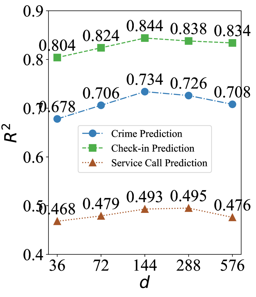
Figure 6: Impact of ${d}$

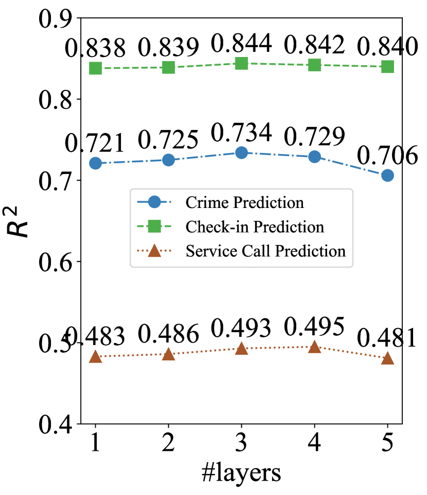
Figure 7: Impact of $\#layers$

VII Conclusion

We proposed a model named HAFusion for urban region representation learning by leveraging human mobility, POI, and land use features. To learn region embeddings from each region feature, we proposed a hybrid attentive feature learning module named HALearning that captures the abundant correlation information between different regions within a single view and across different views. To fuse region embeddings learned from different region features, we further proposed a dual-feature attentive fusion module named DAFusion that encodes higher-order correlations between the regions. To show the effectiveness of HAFusion, we perform three urban prediction tasks using the embeddings learned by HAFusion. The results show that our learned embeddings lead to consistent and up to 31% improvements in prediction accuracy, comparing with those generated by the state-of-the-art models. Meanwhile, our DAFusion module helps improve the quality of the learned embeddings of the existing models by up to 36%.

References

- [1] C. H. Liu, C. Piao, X. Ma, Y. Yuan, J. Tang, G. Wang, and K. K. Leung, “Modeling Citywide Crowd Flows using Attentive Convolutional LSTM,” in ICDE, 2021, pp. 217–228.
- [2] Z. Li, C. Huang, L. Xia, Y. Xu, and J. Pei, “Spatial-Temporal Hypergraph Self-Supervised Learning for Crime Prediction,” in ICDE, 2022, pp. 2984–2996.
- [3] C. Xiao, J. Zhou, J. Huang, H. Zhu, T. Xu, D. Dou, and H. Xiong, “A Contextual Master-Slave Framework on Urban Region Graph for Urban Village Detection,” in ICDE, 2023, pp. 736–748.
- [4] Y. Zheng, L. Capra, O. Wolfson, and H. Yang, “Urban Computing: Concepts, Methodologies, and Applications,” TIST, vol. 5, no. 3, pp. 1–55, 2014.
- [5] J. Zhang, Y. Zheng, and D. Qi, “Deep Spatio-Temporal Residual Networks for Citywide Crowd Flows Prediction,” in AAAI, 2017, pp. 1655–1661.
- [6] Y. Liu, Y. Zheng, Y. Liang, S. Liu, and D. S. Rosenblum, “Urban Water Quality Prediction based on Multi-Task Multi-View Learning,” in IJCAI, 2016, pp. 2576–2582.
- [7] W. Zhuo, K. H. Chiu, J. Chen, J. Tan, E. Sumpena, S.-H. G. Chan, S. Ha, and C.-H. Lee, “Semi-Supervised Learning with Network Embedding on Ambient rf Signals for Geofencing Services,” in ICDE, 2023, pp. 2713–2726.
- [8] Y. Chang, J. Qi, Y. Liang, and E. Tanin, “Contrastive Trajectory Similarity Learning with Dual-Feature Attention,” in ICDE, 2023, pp. 2933–2945.
- [9] P. Yang, H. Wang, Y. Zhang, L. Qin, W. Zhang, and X. Lin, “T3S: Effective Representation Learning for Trajectory Similarity Computation,” in ICDE, 2021, pp. 2183–2188.
- [10] M. Zhang, T. Li, Y. Li, and P. Hui, “Multi-View Joint Graph Representation Learning for Urban Region Embedding,” in IJCAI, 2020, pp. 4431–4437.
- [11] Y. Fu, P. Wang, J. Du, L. Wu, and X. Li, “Efficient Region Embedding with Multi-View Spatial Networks: A Perspective of Locality-Constrained Spatial Autocorrelations,” in AAAI, 2019, pp. 906–913.
- [12] Y. Zhang, Y. Fu, P. Wang, X. Li, and Y. Zheng, “Unifying Inter-Region Autocorrelation and Intra-Region Structures for Spatial Embedding via Collective Adversarial Learning,” in KDD, 2019, pp. 1700–1708.
- [13] J. Du, Y. Zhang, P. Wang, J. Leopold, and Y. Fu, “Beyond Geo-First Law: Learning Spatial Representations via Integrated Autocorrelations and Complementarity,” in ICDM, 2019, pp. 160–169.
- [14] S. Zhou, D. He, L. Chen, S. Shang, and P. Han, “Heterogeneous Region Embedding with Prompt Learning,” in AAAI, 2023, pp. 4981–4989.
- [15] L. Zhang, C. Long, and G. Cong, “Region Embedding With Intra and Inter-View Contrastive Learning,” TKDE, vol. 35, no. 9, pp. 9031–9036, 2023.
- [16] N. Kim and Y. Yoon, “Effective Urban Region Representation Learning using Heterogeneous Urban Graph Attention Network (HUGAT),” arXiv preprint arXiv:2202.09021, 2022.
- [17] P. Jenkins, A. Farag, S. Wang, and Z. Li, “Unsupervised Representation Learning of Spatial Data via Multimodal Embedding,” in CIKM, 2019, pp. 1993–2002.
- [18] Z. Wang, H. Li, and R. Rajagopal, “Urban2Cec: Incorporating Street View Imagery and POIs for Multi-Modal Urban Neighborhood Embedding,” in AAAI, 2020, pp. 1013–1020.
- [19] T. Huang, Z. Wang, H. Sheng, A. Y. Ng, and R. Rajagopal, “Learning Neighborhood Representation from Multi-Modal Multi-Graph: Image, Text, Mobility Graph and Beyond,” arXiv preprint arXiv:2105.02489, 2021.
- [20] H. Wang and Z. Li, “Region Representation Learning via Mobility Flow,” in CIKM, 2017, pp. 237–246.
- [21] Z. Yao, Y. Fu, B. Liu, W. Hu, and H. Xiong, “Representing Urban Functions through Zone Embedding with Human Mobility Patterns,” in IJCAI, 2018, pp. 3919–3925.
- [22] S. Wu, X. Yan, X. Fan, S. Pan, S. Zhu, C. Zheng, M. Cheng, and C. Wang, “Multi-Graph Fusion Networks for Urban Region Embedding,” in IJCAI, 2022, pp. 2312–2318.
- [23] T. Mikolov, K. Chen, G. Corrado, and J. Dean, “Efficient Estimation of Word Representations in Vector Space,” in ICLR-Workshop, 2013.
- [24] P. Wang, Y. Fu, J. Zhang, X. Li, and D. Lin, “Learning Urban Community Structures: A Collective Embedding Perspective with Periodic Spatial-Temporal Mobility Graphs,” TIST, vol. 9, no. 6, pp. 1–28, 2018.
- [25] W. Huang, D. Zhang, G. Mai, X. Guo, and L. Cui, “Learning Urban Region Representations with POIs and Hierarchical Graph Infomax,” ISPRS Journal of Photogrammetry and Remote Sensing, vol. 196, pp. 134–145, 2023.
- [26] Y. Li, W. Huang, G. Cong, H. Wang, and Z. Wang, “Urban Region Representation Learning with OpenStreetMap Building Footprints,” in KDD, 2023, pp. 1363–1373.
- [27] T. Chen, S. Kornblith, M. Norouzi, and G. Hinton, “A Simple Framework for Contrastive Learning of Visual Representations,” in ICML, 2020, pp. 1597–1607.
- [28] N. Jean, S. Wang, A. Samar, G. Azzari, D. Lobell, and S. Ermon, “Tile2vec: Unsupervised Representation Learning for Spatially Distributed Data,” in AAAI, 2019, pp. 3967–3974.
- [29] Y. Zhao, J. Qi, B. D. Trisedya, Y. Su, R. Zhang, and H. Ren, “Learning Region Similarities via Graph-based Deep Metric Learning,” TKDE, vol. 35, no. 10, pp. 10 237–10 250, 2023.
- [30] J. Li, H. Yong, B. Zhang, M. Li, L. Zhang, and D. Zhang, “A Probabilistic Hierarchical Model for Multi-View and Multi-Feature Classification,” in AAAI, 2018, pp. 3498–3505.
- [31] J. Zhao, X. Xie, X. Xu, and S. Sun, “Multi-View Learning Overview: Recent Progress and New Challenges,” Information Fusion, vol. 38, pp. 43–54, 2017.
- [32] C. Zhang, H. Fu, Q. Hu, X. Cao, Y. Xie, D. Tao, and D. Xu, “Generalized Latent Multi-View Subspace Clustering,” TPAMI, vol. 42, no. 1, pp. 86–99, 2018.
- [33] Y. Li, M. Yang, and Z. Zhang, “A Survey of Multi-View Representation Learning,” TKDE, vol. 31, no. 10, pp. 1863–1883, 2018.
- [34] Y. Fu, H. Xiong, Y. Ge, Z. Yao, Y. Zheng, and Z.-H. Zhou, “Exploiting Geographic Dependencies for Real Estate Appraisal: A Mutual Perspective of Ranking and Clustering,” in KDD, 2014, pp. 1047–1056.
- [35] T. N. Kipf and M. Welling, “Semi-Supervised Classification with Graph Convolutional Cetworks,” in ICLR, 2017.
- [36] P. Veličković, G. Cucurull, A. Casanova, A. Romero, P. Lio, and Y. Bengio, “Graph Attention Networks,” in ICLR, 2018.
- [37] X. Wang, H. Ji, C. Shi, B. Wang, Y. Ye, P. Cui, and P. S. Yu, “Heterogeneous Graph Attention Network,” in WWW, 2019, pp. 2022–2032.
- [38] M. Schultz and T. Joachims, “Learning a Distance Metric from Relative Comparisons,” in NeurIPS, 2003, pp. 41–48.
- [39] OpenStreetMap. https://www.openstreetmap.org/.
- [40] New York Dataset. https://opendata.cityofnewyork.us/.
- [41] Chicago Dataset. https://data.cityofchicago.org/.
- [42] San Francisco Dataset. https://datasf.org/opendata/.
- [43] A. Vaswani, N. Shazeer, N. Parmar, J. Uszkoreit, L. Jones, A. N. Gomez, Ł. Kaiser, and I. Polosukhin, “Attention is All You Need,” in NeurIPS, 2017, pp. 6000–6010.
- [44] M.-H. Guo, Z.-N. Liu, T.-J. Mu, and S.-M. Hu, “Beyond Self-Attention: External Attention using Two Linear Layers for Visual Tasks,” TPAMI, vol. 45, no. 5, pp. 5436–5447, 2022.
- [45] Foursquare Dataset. https://sites.google.com/site/yangdingqi/home/foursquare-dataset.
- [46] P. G. Ward, Z. He, R. Zhang, and J. Qi, “Real-time continuous intersection joins over large sets of moving objects using graphic processing units,” VLDBJ, vol. 23, no. 6, p. 965–985, 2014.
- [47] Y. Wang, R. Zhang, C. Xu, J. Qi, Y. Gu, and G. Yu, “Continuous visible k nearest neighbor query on moving objects,” Information Systems, vol. 44, pp. 1–21, 2014.