Second- and third-order properties of multidimensional Langevin equations

Abstract.

Recent work has addressed the problem of inferring Langevin dynamics from data. In this work, we address the problem of relating terms in the Langevin equation to statistical properties, such as moments of the probability density function and of the probability current density, as well as covariance functions. We first review the case of linear Gaussian dynamics, and then consider extensions beyond this simple case. We address the question of quantitative significance of effects. We also analyze underdamped (second-order) processes, specifically in the limit where dynamics in state space is almost Markovian.

1. Introduction

Langevin equations, or equivalently Fokker–Planck equations, play an important role in stochastic modeling of biological systems, from animal locomotion [1] to cell migration [2]. These stochastic differential equations describe Markov processes in continuous time having values in a continuous state space with continuous paths [3]. The simplest process admitting a stationary probability distribution is a linear Gaussian process where drift is a linear function of the state variables, and diffusion matrix is constant. Such processes have been discussed in [4], where their properties are analyzed in an coordinate-invariant manner. In this paper, we elaborate on the linear case and extend this analysis to processes having nonlinear drift and inhomogeneous diffusion.

Probability currents are related to entropy production in the case where the state variables are even under time reversal [5]. It has been proposed to use state-space coarse-graining to analyze probability currents [6]. However, this approach is not ideal for purposes of statistical testing, as it requires arbitrarily choosing a (closed) path around which to calculate the probability flux (see [7]). In addition, it is data-hungry in high dimension. Instead, a quantity known as angular momentum, also known as twice the stochastic area, has been proposed to quantify circulation in linear models [8]. In this paper, we extend this approach to nonlinear circulations.

Recent work has addressed the problem of inferring Langevin dynamics from data [9, 10]. The amount of information that can be statistically resolved depends on the amount of data collected [11, 12]. However, just because effects can be statistically resolved does not mean that they are quantitatively significant. Effects of interest include non-Gaussian probability distributions, non-vanishing probability currents, and inhomogeneous diffusion. We introduce a framework in which to evaluate the quantitative significance of such effects, invariant under linear transformations of the state coordinates.

We discuss the case where some variables do not admit stationary probability distributions. We also discuss the case where some variables are odd under time reversal. We discuss experimentally measurable covariance functions, and prove that they are time-reversible under certain assumptions and suitable approximations. We also discuss quantitative comparison of theoretical and experimental covariance functions.

Finally, we consider underdamped (second-order) processes, specifically in the limit where dynamics in state space is almost Markovian.

2. Linear Gaussian stationary systems

2.1. Preliminaries: Definition, covariance functions, and detailed balance

We consider the following Langevin system:

(1) $$\dot{\mathbf{x}}=\mathbf{A}\mathbf{x}+\boldsymbol{\xi},\quad\langle\boldsymbol{\xi}(t)\rangle=\mathbf{0},\quad\langle\boldsymbol{\xi}(t)\boldsymbol{\xi}(t^{\prime})^{\mathsf{T}}\rangle=2\mathbf{D}\delta(t-t^{\prime}),$$

with $\mathbf{A}$ and $\mathbf{D}$ constant, and $\delta(\cdot)$ is Dirac delta function. The covariance matrix $\mathbf{C}:=\langle\mathbf{x}\mathbf{x}^{\mathsf{T}}\rangle$ is determined from the Lyapunov equation:

(2) $$\mathbf{A}\mathbf{C}+\mathbf{C}\mathbf{A}^{\mathsf{T}}+2\mathbf{D}=\mathbf{0},$$

which can be solved using tensor notation and Einstein summation notation as:

(3) $$C^{ij}=-2\left[{(\mathbf{A}\otimes\mathds{1}+\mathds{1}\otimes\mathbf{A})^{-1}}\right]^{ij}_{kl}D^{kl}.$$

where $\mathds{1}$ denotes the identity matrix of appropriate dimension. When comparing to experimental data, this relation is not to be considered as a test of the linear model, as it is a simple consequence of stationarity of $\mathbf{x}$ and the model fit, by Itô’s lemma:

(4) $$\mathbf{0}=\frac{\mathrm{d}}{\mathrm{d}t}\langle\mathbf{x}(t)\mathbf{x}(t)^{\mathsf{T}}\rangle=\langle\dot{\mathbf{x}}(t)\mathbf{x}(t)^{\mathsf{T}}\rangle+\langle\mathbf{x}(t)\dot{\mathbf{x}}(t)^{\mathsf{T}}\rangle+\left\langle{\frac{\mathrm{d}[\mathbf{x},\mathbf{x}^{\mathsf{T}}](t)}{\mathrm{d}t}}\right\rangle$$

where the time-derivative is interpreted in the Itô sense, and $[\cdot,\cdot]$ is the covariation. In fact, the above follows simply from a rearrangement of terms:

(5) $$\langle(\mathbf{x}(\tau)-\mathbf{x}(0))(\mathbf{x}(\tau)-\mathbf{x}(0))^{\mathsf{T}}\rangle =\langle\mathbf{x}(\tau)\mathbf{x}(\tau)^{\mathsf{T}}-\mathbf{x}(0)\mathbf{x}(\tau)^{\mathsf{T}}\rangle-\langle(\mathbf{x}(\tau)-\mathbf{x}(0))\mathbf{x}(0)^{\mathsf{T}}\rangle$$

$$=\langle\mathbf{x}(0)(\mathbf{x}(0)-\mathbf{x}(\tau))^{\mathsf{T}}\rangle-\langle(\mathbf{x}(\tau)-\mathbf{x}(0))\mathbf{x}(0)^{\mathsf{T}}\rangle$$

upon dividing by $\tau$ and taking $\tau\to 0$, where we used $\langle\mathbf{x}(\tau)\mathbf{x}(\tau)^{\mathsf{T}}\rangle=\langle\mathbf{x}(0)\mathbf{x}(0)^{\mathsf{T}}\rangle$. (In certain cases, care must be taken when evaluating these expressions; see Appendix B.)

Of interest is the covariance function:

(6) $$\langle\mathbf{x}(\tau)\mathbf{x}(0)^{\mathsf{T}}\rangle=e^{\mathbf{A}\tau}\mathbf{C},$$

where $\tau\geq 0$ is always assumed. Note that this is satisfied even in the case of non-constant diffusion.

Of interest also is the condition for detailed balance. A requirement for detailed balance is that the covariance function is symmetric, $\langle\mathbf{x}(\tau)\mathbf{x}(0)^{\mathsf{T}}\rangle=\langle\mathbf{x}(0)\mathbf{x}(\tau)^{\mathsf{T}}\rangle$. By differentiating with respect to $\tau$, we get $\mathbf{A}\mathbf{C}=\mathbf{C}\mathbf{A}^{\mathsf{T}}$. To gain insight into this relation, we switch to “covariance-identity” coordinates in which $\mathbf{C}=\mathds{1}$ [13]. In such a basis, $\mathbf{A}$ is symmetric, which means it is diagonalizable by an orthogonal basis. In these coordinates, an orthogonal basis means uncorrelated components. By the Lyapunov equation, $\mathbf{D}$ must also be diagonal in this basis. Hence the system decomposes into a number of noninteracting one-dimensional linear systems [4]. Ref. [4] also contains good discussions about general properties of linear Gaussian systems.

The Lyapunov equation implies a relationship between the eigenvalues of $\mathbf{A}$ and of $\mathbf{D}\mathbf{C}^{-1}$. We work in a coordinate system in which $\mathbf{C}=\mathds{1}$. Let $\lambda$ be an eigenvalue of $\mathbf{A}$ and $\mathbf{v}$ be a corresponding eigenvector. Then:

(7) $$\mathbf{v}^{\mathsf{H}}\mathbf{D}\mathbf{v}=-\mathbf{v}^{\mathsf{H}}\left({\frac{\mathbf{A}+\mathbf{A}^{\mathsf{T}}}{2}}\right)\mathbf{v}=-(\Re\lambda)(\mathbf{v}^{\mathsf{H}}\mathbf{v}),$$

therefore $-\Re\lambda$ is bounded by the smallest and largest eigenvalues of $\mathbf{D}$ [14].

2.2. Comparison of experimental data with theoretical predictions

Now, we turn to the question of comparing experimental data and theoretical predictions under a linear model. We may consider comparing the deviation of $\langle\mathbf{x}(\tau)\mathbf{x}(0)^{\mathsf{T}}\rangle$ to $\mathbf{C}$. That is, if we consider a whitened dataset for which $\mathbf{C}=\mathds{1}$, the entries of the deviation matrix in these coordinates should be compared to unity. For a coordinate-independent description, we may look at the symmetric and antisymmetric parts of the deviation matrix and multiply these on the right by $\mathbf{C}^{-1}$, and inspect the eigenvalues, which are purely real and imaginary in the symmetric and antisymmetric cases, respectively.

We denote the deviation $\mathbf{M}:=\langle\mathbf{x}\mathbf{x}^{\mathsf{T}}\rangle_{\text{expt}}-\mathbf{C}_{\text{theo}}$. From now on we suppress the “theo” subscript and treat $\mathbf{C}$ as fixed. We may consider the eigenvalues of $\mathbf{M}\mathbf{C}^{-1}$, which are real since we have a matrix that is symmetric in coordinates in which $\mathbf{C}=\mathds{1}$. We may imagine an ensemble of stochastic systems, in which deviations of $\mathbf{M}$ from $\mathbf{0}$ are permitted. We may ask the question of what a suitable variance of $\mathbf{M}$ would be. We may then compare the elements of $\mathbf{M}$ to the square root of the “ensemble variance”. For biological applications, a factor of 0.3 or more may be considered significant.

In the presence of symmetries, some components of $\mathbf{M}$ may be constrained to be 0. Absent such restrictions, we may consider the putative relation:

(8) $$M^{ij}M^{i^{\prime}j^{\prime}}\sim C^{ii^{\prime}}C^{jj^{\prime}}.$$

where $\sim$ denotes ensemble expectation. We may treat $(i,j)$ as a single index and similarly for $(i^{\prime},j^{\prime})$, and multiply the l.h.s. (left-hand side) by the matrix inverse of the r.h.s. (right-hand side). We denote by $\boldsymbol{\Gamma}$ the resulting matrix:

(9) $$\Gamma^{ij}_{i^{\prime}j^{\prime}}:=M^{ij}M^{kl}C^{-1}_{i^{\prime}k}C^{-1}_{j^{\prime}l}.$$

It so happens that $\boldsymbol{\Gamma}$ has at most one non-zero eigenvalue $\mu$, which is equal to its trace. (In future sections, this will not necessarily be the case.) We have:

(10) $$\operatorname{tr}(\boldsymbol{\Gamma})=M^{ij}M^{i^{\prime}j^{\prime}}C^{-1}_{ii^{\prime}}C^{-1}_{jj^{\prime}}=\operatorname{tr}((\mathbf{M}\mathbf{C}^{-1})^{2}).$$

Operating in “covariance-identity” coordinates, it is seen that $M^{ij}$ where $i\neq j$ is counted double as compared to when $i=j$. We give an example of this in two dimensions. Changing coordinates to $x^{\prime}:=(x+y)/\sqrt{2}$ and $y^{\prime}=(y-x)/\sqrt{2}$, we see that:

(11) $$\langle{x^{\prime}}^{2}\rangle =1+\langle xy\rangle,$$

(12) $$\langle{y^{\prime}}^{2}\rangle =1-\langle xy\rangle,$$

(13) $$\langle x^{\prime}y^{\prime}\rangle =0.$$

This shows indeed that deviations in $\langle xy\rangle$ should be counted double compared to deviations in $\langle x^{2}\rangle$ or $\langle y^{2}\rangle$.

There is, however, a problem with Eq. (8), which is that it does not obey symmetry in the indices. We may denote by $v_{ij}$ a left eigenvector of $\boldsymbol{\Gamma}$ with eigenvalue $\mu$, which satisfies:

(14) $$v_{ij}M^{ij}M^{i^{\prime}j^{\prime}}=\mu v_{ij}C^{ii^{\prime}}C^{jj^{\prime}}.$$

Since this is symmetric in $(i^{\prime},j^{\prime})$, we can write this as:

(15) $$v_{ij}M^{ij}M^{i^{\prime}j^{\prime}}=\mu v_{ij}\frac{C^{ii^{\prime}}C^{jj^{\prime}}+C^{ij^{\prime}}C^{ji^{\prime}}}{2}.$$

Now if we neglect permutations in $(i,j)$ and $(i^{\prime},j^{\prime})$, we can see that the matrix product of $M^{ij}M^{i^{\prime}j^{\prime}}$ with the matrix inverse of the quantity following $v_{ij}$ on the r.h.s. of Eq. (15) has the same eigenvalue $\mu$. Thus we may consider instead of Eq. (8) the relation:

(16) $$M^{ij}M^{i^{\prime}j^{\prime}}\sim\frac{C^{ii^{\prime}}C^{jj^{\prime}}+C^{ij^{\prime}}C^{ji^{\prime}}}{2}.$$

We may assess the quantitative significance of a single element $M^{ij}$ by setting $i^{\prime}=i$, $j^{\prime}=j$ in the above, taking square roots, and comparing. For an assessment of all $M^{ij}$ collectively, we may calculate the trace of $\boldsymbol{\Gamma}$ according to this prescription:

(17) $$\operatorname{tr}(\boldsymbol{\Gamma})=\mu\sim\frac{d(d+1)}{2},$$

where $d$ is the dimension. The r.h.s. is the number of degrees of freedom in $\mathbf{M}$, accounting for symmetry. If $\sqrt{\mu}$ is comparable to $\sqrt{d(d+1)/2}$, then it may be considered quantitatively significant.

Now we turn to covariance functions with a time-lag. We may again denote the deviation $\mathbf{M}:=\langle\mathbf{x}(\tau)\mathbf{x}(0)^{\mathsf{T}}\rangle_{\text{expt}}-\langle\mathbf{x}(\tau)\mathbf{x}(0)^{\mathsf{T}}\rangle_{\text{theo}}$. We can separate $\mathbf{M}$ into symmetric and antisymmetric components:

(18) $$\mathbf{S} :=\frac{\mathbf{M}+\mathbf{M}^{\mathsf{T}}}{2},$$

(19) $$\mathbf{T} :=\frac{\mathbf{M}-\mathbf{M}^{\mathsf{T}}}{2}.$$

Then $\mathbf{S}\mathbf{C}^{-1}$ and $\mathbf{T}\mathbf{C}^{-1}$ have purely real and purely imaginary eigenvalues, respectively. We have:

(20) $$S^{ij}S^{i^{\prime}j^{\prime}}C^{-1}_{ii^{\prime}}C^{-1}_{jj^{\prime}} =\operatorname{tr}((\mathbf{S}\mathbf{C}^{-1})^{2}),$$

(21) $$T^{ij}T^{i^{\prime}j^{\prime}}C^{-1}_{ii^{\prime}}C^{-1}_{jj^{\prime}} =-\operatorname{tr}((\mathbf{T}\mathbf{C}^{-1})^{2}).$$

Straightforward calculation reveals that:

(22) $$(S^{ij}S^{i^{\prime}j^{\prime}}+T^{ij}T^{i^{\prime}j^{\prime}})C^{-1}_{ii^{\prime}}C^{-1}_{jj^{\prime}}=M^{ij}M^{i^{\prime}j^{\prime}}C^{-1}_{ii^{\prime}}C^{-1}_{jj^{\prime}}.$$

The above equality relates its r.h.s. to the sums of the squared eigenvalues of $\mathbf{S}\mathbf{C}^{-1}$ and $\mathbf{T}\mathbf{C}^{-1}$. Since there is no symmetry requirement for $\mathbf{M}$, we may take the components of $\mathbf{M}$ as obeying Eq. (8), in which case the components of $\mathbf{S}$ and $\mathbf{T}$ follow:

(23) $$S^{ij}S^{i^{\prime}j^{\prime}} \sim\frac{C^{ii^{\prime}}C^{jj^{\prime}}+C^{ij^{\prime}}C^{ji^{\prime}}}{2},$$

(24) $$T^{ij}T^{i^{\prime}j^{\prime}} \sim\frac{C^{ii^{\prime}}C^{jj^{\prime}}-C^{ij^{\prime}}C^{ji^{\prime}}}{2}.$$

This implies:

(25) $$S^{ij}S^{i^{\prime}j^{\prime}}C^{-1}_{ii^{\prime}}C^{-1}_{jj^{\prime}} \sim\frac{d(d+1)}{2},$$

(26) $$T^{ij}T^{i^{\prime}j^{\prime}}C^{-1}_{ii^{\prime}}C^{-1}_{jj^{\prime}} \sim\frac{d(d-1)}{2}.$$

The r.h.s.’s correspond to the degrees of freedom in $\mathbf{S}$ and $\mathbf{T}$, respectively. If $\sqrt{M^{ij}M^{i^{\prime}j^{\prime}}C^{-1}_{ii^{\prime}}C^{-1}_{jj^{\prime}}}$ is comparable to $d$, then $\mathbf{M}$ may be considered (collectively) quantitatively significant.

For the case of complex variables, see Appendix A.

2.3. Probability current density and angular momentum

At stationarity (which is assumed throughout), the probability density is $p(\mathbf{x})\propto\exp\left({-\frac{1}{2}\mathbf{x}^{\mathsf{T}}\mathbf{C}^{-1}\mathbf{x}}\right)$ and the probability current density is $\mathbf{J}(\mathbf{x})=\boldsymbol{\Omega}\mathbf{x}p(\mathbf{x})$, where $\boldsymbol{\Omega}=\mathbf{A}+\mathbf{D}\mathbf{C}^{-1}$. The matrix $\boldsymbol{\Omega}$ is traceless and has purely imaginary eigenvalues [13] which define stochastic rotation frequencies, and the corresponding complex eigenvectors define planes in which breaking of detailed balance occurs.

The dynamics of the linear system is determined by the matrices $\mathbf{A}$ and $\mathbf{D}$. However, to characterize the system based on quantities even and odd under time-reversal, we may consider the angular momentum matrix:

(27) $$\mathbf{L}:=\lim_{\tau\to 0}\frac{\langle\mathbf{x}(0)\mathbf{x}(\tau)^{\mathsf{T}}-\mathbf{x}(\tau)\mathbf{x}(0)^{\mathsf{T}}\rangle}{\tau}=\langle\mathbf{x}\dot{\mathbf{x}}^{\mathsf{T}}-\dot{\mathbf{x}}\mathbf{x}^{\mathsf{T}}\rangle=\mathbf{C}\mathbf{A}^{\mathsf{T}}-\mathbf{A}\mathbf{C},$$

where the time-derivatives are interpreted in Itô sense. We also have $\mathbf{L}=2\langle\mathbf{x}\circ\dot{\mathbf{x}}^{\mathsf{T}}\rangle$ where the time-derivative is interpreted in Stratonovich sense. The system may now be characterized in terms of $\mathbf{C}$, $\mathbf{L}$, and $\mathbf{D}$.

Now we specialize to the two-dimensional case, where $\mathbf{x}=(x,y)^{\mathsf{T}}$. Here, $\boldsymbol{\Omega}$ has a single pair of purely imaginary eigenvalues $\pm i\omega_{\mathrm{stoch}}$. The angular momentum is $L(x,y):=\langle x\dot{y}-\dot{x}y\rangle$ (where the time-derivatives are interpreted in Itô sense). The angular momentum is related to the matrix $\boldsymbol{\Omega}$ by the relation

(28) $$\mathbf{A}\mathbf{C}-\mathbf{C}\mathbf{A}^{\mathsf{T}}=\begin{pmatrix}0&-L\\ L&0\end{pmatrix}=2\boldsymbol{\Omega}\mathbf{C},$$

and upon taking determinants, we get

(29) $$\omega_{\mathrm{stoch}}=\frac{L}{2\sqrt{\det(\mathbf{C})}}.$$

In the three-dimensional case, $\boldsymbol{\Omega}$ has at most a single pair of non-zero purely imaginary eigenvalues, and the stochastic rotation frequency is half the magnitude of the angular momentum vector evaluated in “covariance-identity” coordinates.

The stochastic rotation frequency where $\mathbf{A}$ has two real eigenvalues has been computed in [15] and is easily derived from the above formula in coordinates where:

(30) $$\mathbf{A}=\begin{pmatrix}-\lambda_{x}&0\\ 0&-\lambda_{y}\end{pmatrix},$$

where $\lambda_{x},\lambda_{y}>0$. For completeness, the result is:

(31) $$\omega_{\mathrm{stoch}}=(\lambda_{x}-\lambda_{y})D^{xy}\left[{\frac{(\lambda_{x}+\lambda_{y})^{2}}{\lambda_{x}\lambda_{y}}D^{xx}D^{yy}-4(D^{xy})^{2}}\right]^{-1/2}.$$

The stochastic rotation frequency is bounded above by the geometric mean of the relaxation rates, $\left|\omega_{\mathrm{stoch}}\right|\leq\sqrt{\lambda_{x}\lambda_{y}}$, with equality attained when $\mathbf{D}$ is singular ($D^{xx}D^{yy}=(D^{xy})^{2}$). Now, we turn to the case where $\mathbf{A}$ has a pair of complex conjugate eigenvalues. Without loss of generality, after a change of coordinates, we may write:

(32) $$\mathbf{A}=\begin{pmatrix}-\lambda&-\omega\\ \omega&-\lambda\end{pmatrix},\quad D^{xy}=0,$$

where $\lambda>0$, $\omega>0$. Here, $L=\omega\operatorname{tr}(\mathbf{C})$, which gives

(33) $$\omega_{\mathrm{stoch}}=\frac{\omega\operatorname{tr}(\mathbf{C})}{2\sqrt{\det(\mathbf{C})}}.$$

Since $\mathbf{C}$ has real eigenvalues, $(\operatorname{tr}(\mathbf{C}))^{2}-4\det(\mathbf{C})\geq 0$ and therefore $\omega_{\mathrm{stoch}}\geq\omega$. Equality holds if and only if $\mathbf{C}$ is a multiple of the identity.

To continue the calculation, we solve the Lyapunov equation $\mathbf{A}\mathbf{C}+\mathbf{C}\mathbf{A}^{\mathsf{T}}=-2\mathbf{D}$ for $\mathbf{C}$ and obtain:

(34) $$\mathbf{C}=\frac{1}{\lambda}\begin{pmatrix}D^{xx}-\delta/2&\lambda\delta/{2\omega}\\ \lambda\delta/{2\omega}&D^{yy}+\delta/2\end{pmatrix},\quad\delta:=\frac{D^{xx}-D^{yy}}{1+\lambda^{2}/\omega^{2}}.$$

This gives:

(35) $$\omega_{\mathrm{stoch}}=\omega(D^{xx}+D^{yy})\left[{4D^{xx}D^{yy}+\frac{(D^{xx}-D^{yy})^{2}}{1+\lambda^{2}/\omega^{2}}}\right]^{-1/2}.$$

It can be seen from elementary algebra that $\omega_{\mathrm{stoch}}\leq\sqrt{\lambda^{2}+\omega^{2}}$, with equality holding if and only if $D^{xx}D^{yy}=0$, i.e., the matrix $\mathbf{D}$ is singular.

As noted in [15], the stochastic rotation frequencies can be experimentally measured by averaging over angular motions. We can formally prove this by working in coordinates where $\mathbf{C}=\mathds{1}$ and use Stratonovich calculus to transform to polar coordinates $(r,\phi)$. We have:

(36) $${}\circ\mathrm{d}\phi=\frac{\cos\phi\circ\mathrm{d}y-\sin\phi\circ\mathrm{d}x}{r}=\frac{x\circ\mathrm{d}y-y\circ\mathrm{d}x}{r^{2}}$$

Because the phase-space velocity $\mathbf{J}(\mathbf{x})/p(\mathbf{x})$ is linear, $\langle{}\circ\dot{\phi}\mid r,\phi\rangle$ is independent of $r$. Also, by our choice of coordinates, the distribution of $\mathbf{x}$ is isotropic, which means that $r$ is independent of $\phi$. Thus $L=\langle r^{2}\circ\dot{\phi}\rangle=\langle r^{2}\rangle\langle\dot{\phi}\rangle=2\langle\dot{\phi}\rangle$, as desired. We have numerically verified this for a system obeying Eq. (32) where $\lambda=\omega=1$, $D^{xx}=1$, $D^{yy}=10$. We simulated this system using Euler–Maruyama discretization with $\Delta t=0.005$ for 1000 time-units. We see that the measured stochastic rotation frequency is in agreement with the theoretical value of 1.23 (Fig. 1).

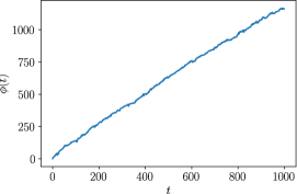
Figure 1. Measured stochastic rotation frequency.

At this point, we still do not have a good dimensionless measure of when broken detailed balance is quantitatively significant. To do this, we turn to a modified definition of gain matrix [13, 4]:

(37) $$\mathbf{H}:=\mathds{1}+\mathbf{A}\mathbf{C}\mathbf{D}^{-1}=(\mathbf{A}\mathbf{C}-\mathbf{C}\mathbf{A}^{\mathsf{T}})(2\mathbf{D})^{-1}.$$

where the last equality follows from the Lyapunov equation. The entropy production rate $\dot{S}$ is related to $\mathbf{H}$ as $\dot{S}=-\operatorname{tr}(\mathbf{A}\mathbf{H})$ [13]. By a similar argument as in [13], in coordinates in which $\mathbf{D}=\mathds{1}$, we see that $\mathbf{H}$ is antisymmetric and therefore, like $\boldsymbol{\Omega}$, has purely imaginary complex conjugate eigenvalues. As an alternative derivation, following [3], we may consider that $\mathbf{D}^{-1/2}\mathbf{H}\mathbf{D}^{1/2}$ is antisymmetric and therefore $\mathbf{H}$ is similar to an antisymmetric matrix. In two dimensions the (dimensionless) eigenvalues $\pm ih$ are given by a simple formula similar to that of $\omega_{\mathrm{stoch}}$:

(38) $$h=\frac{L}{2\sqrt{\det(\mathbf{D})}}.$$

If $h$ is at least comparable to unity, then we consider that broken detailed balance is significant. (We may understand the factor of 2 in the definition of $\mathbf{H}$ by considering that the symmetric part of $\mathbf{A}\mathbf{C}$ is $-\mathbf{D}$ by the Lyapunov equation, so the antisymmetric part should be compared to $\mathbf{D}$.) We may illustrate this on the two examples above. For two real eigenvalues of $\mathbf{A}$,

(39) $$h=\frac{\lambda_{x}-\lambda_{y}}{\lambda_{x}+\lambda_{y}}\cdot\frac{D^{xy}}{\sqrt{D^{xx}D^{yy}-(D^{xy})^{2}}}.$$

For broken detailed balance to be significant, one possibility is that $\lambda_{x}$ is far away from $\lambda_{y}$ and $D^{xy}/\sqrt{D^{xx}D^{yy}}$ is far from zero. The other possibility is that $D^{xy}\approx\sqrt{D^{xx}D^{yy}}$. The latter possibility allows for $\lambda_{x}\approx\lambda_{y}$, in which case $\mathbf{C}$ as well as $\mathbf{D}$ is almost singular in the chosen coordinates. In coordinates where $\mathbf{C}$ is well-conditioned, this corresponds to the case where $\mathbf{A}$ almost has a generalized eigenvector.

For the case of complex conjugate eigenvalues of $\mathbf{A}$,

(40) $$h=\frac{\omega}{\lambda}\cdot\frac{D^{xx}+D^{yy}}{2\sqrt{D^{xx}D^{yy}}}.$$

We see that $h\geq\omega/\lambda$. Again, there are two possibilities for significant broken detailed balance. One possibility is that $\omega/\lambda$ is significant compared to unity. The other possibility is $\sqrt{D^{xx}}\ll\sqrt{D^{yy}}$ (or vice versa), which allows for the possibility that $\omega\ll\lambda$. As before, this corresponds to the case where $\mathbf{A}$ almost has a generalized eigenvector.

For angular momenta of $d$-dimensional systems, we may follow the part of the previous discussion pertaining to the antisymmetric part, except with $\mathbf{C}$ replaced by $2\mathbf{D}$, i.e.:

(41) $$L^{ij}L^{i^{\prime}j^{\prime}}\sim 2(D^{ii^{\prime}}D^{jj^{\prime}}-D^{ij^{\prime}}D^{ji^{\prime}}).$$

Note that when summing the squared eigenvalues of $\mathbf{H}$, the eigenvalues occur in pairs. If the time-step is not small and angular momenta are measured using discrete time, then on the r.h.s. of the above, it may be suitable to use instead discrete-time estimators of the diffusion.

2.4. Estimation of $\mathbf{A}$ from trajectories

We now consider the estimation of $\mathbf{A}$ in multiple dimensions. It has been shown that for estimation of the force field from stochastic trajectories, there is a finite rate at which information can be extracted [9]. This work has shown that the mean coefficient of the inferred force field $\widehat{\mathbf{A}}\mathbf{x}$ is $\langle\widehat{\mathbf{A}}\rangle=\mathbf{A}$ with correction $\mathcal{O}(T^{-1})$. However, they do not discuss the dependence of $\langle\widehat{\mathbf{A}}\rangle$ on dimension $d$. Eq. (C11) in [9] is summed over basis function index $\alpha$, and we may guess Eq. (C13) to be of order $\mathcal{O}(d^{3})$, leaving a $\mathcal{O}(d)$ bias for the inferred force field coefficient. We explicitly calculate the bias and variance of $\widehat{\mathbf{A}}$ for a $d$-dimensional linear system in which $-\mathbf{A}=\mathbf{D}=\mathbf{C}=\mathds{1}$. According to the information-theoretic criterion in [9], the force field should start to be resolved for a trajectory length of 2 time-units. The value of $\widehat{\mathbf{A}}$ inferred from a trajectory of duration $T$ is:

(42) $$\widehat{\mathbf{A}}(T)=\left({\int_{0}^{T}\mathrm{d}\tau\,\dot{\mathbf{x}}(\tau)\mathbf{x}(\tau)^{\mathsf{T}}}\right)\left({\int_{0}^{T}\mathrm{d}\tau^{\prime}\,\mathbf{x}(\tau^{\prime})\mathbf{x}(\tau^{\prime})^{\mathsf{T}}}\right)^{-1}.$$

We now define:

(43) $$\widehat{\mathbf{C}}(T):=\frac{1}{T}\int_{0}^{T}\mathrm{d}\tau\,\mathbf{x}(\tau)\mathbf{x}(\tau)^{\mathsf{T}}.$$

Denoting $\Delta\widehat{\mathbf{C}}(T):=\widehat{\mathbf{C}}(T)-\mathds{1}$, we expand:

(44) $$\widehat{\mathbf{C}}(T)^{-1}=(\mathds{1}+\Delta\widehat{\mathbf{C}}(T))^{-1}=\sum_{n=0}^{\infty}(-1)^{n}(\Delta\widehat{\mathbf{C}}(T))^{n}.$$

The $n=0$ term contributes $-\mathds{1}$ to $\langle\widehat{\mathbf{A}}(T)\rangle$. For the contribution of the $n=1$ term, we have from Gaussianity and Isserlis’s theorem:

(45) $$\frac{1}{T^{2}}\int_{0}^{T}\mathrm{d}\tau\int_{0}^{T}\mathrm{d}\tau^{\prime}\,\langle\dot{x}^{i}(\tau)x^{j}(\tau)(x^{k}(\tau^{\prime})x^{l}(\tau^{\prime})-\delta^{kl})\rangle$$

$$\quad{}=\frac{1}{T^{2}}\int_{0}^{T}\mathrm{d}\tau\int_{0}^{T}\mathrm{d}\tau^{\prime}\,(\langle\dot{x}^{i}(\tau)x^{k}(\tau^{\prime})\rangle\langle x^{j}(\tau)x^{l}(\tau^{\prime})\rangle+\langle\dot{x}^{i}(\tau)x^{l}(\tau^{\prime})\rangle\langle x^{j}(\tau)x^{k}(\tau^{\prime})\rangle).$$

We have:

(46) $$\langle x^{i}(\tau)x^{j}(\tau^{\prime})\rangle =\delta^{ij}e^{-|\tau-\tau^{\prime}|},$$

(47) $$\langle\dot{x}^{i}(\tau)x^{j}(\tau^{\prime})\rangle =\delta^{ij}e^{-|\tau-\tau^{\prime}|}\begin{cases}-1,\quad\tau^{\prime}\leq\tau,\\ +1,\quad\tau^{\prime}>\tau,\end{cases}$$

where $\delta$ is Kronecker delta. Thus the contribution of the $n=1$ term vanishes. For the contribution of the $n=2$ term, we have:

(48) $$\left\langle{\frac{1}{T}\int_{0}^{T}\mathrm{d}\tau\,\dot{x}^{i}(\tau)x^{j}(\tau)(\Delta\widehat{C}(T))^{kl}(\Delta\widehat{C}(T))^{k^{\prime}l^{\prime}}}\right\rangle=\frac{1}{T^{3}}\int_{0}^{T}\mathrm{d}\tau\int_{0}^{T}\mathrm{d}\tau^{\prime}\int_{0}^{T}\mathrm{d}\tau^{\prime\prime}$$

$$\quad\Big{[}{\langle\dot{x}^{i}(\tau)x^{j}(\tau)\rangle(\langle x^{k}(\tau^{\prime})x^{k^{\prime}}(\tau^{\prime\prime})\rangle\langle x^{l}(\tau^{\prime})x^{l^{\prime}}(\tau^{\prime\prime})\rangle+\langle x^{k}(\tau^{\prime})x^{l^{\prime}}(\tau^{\prime\prime})\rangle\langle x^{l}(\tau^{\prime})x^{k^{\prime}}(\tau^{\prime\prime})\rangle)}\Big{.}$$

$$\qquad{}+\langle\dot{x}^{i}(\tau)x^{k}(\tau^{\prime})\rangle(\langle x^{j}(\tau)x^{k^{\prime}}(\tau^{\prime\prime})\rangle\langle x^{l}(\tau^{\prime})x^{l^{\prime}}(\tau^{\prime\prime})\rangle+\langle x^{j}(\tau)x^{l^{\prime}}(\tau^{\prime\prime})\rangle\langle x^{l}(\tau^{\prime})x^{k^{\prime}}(\tau^{\prime\prime})\rangle)$$

$$\qquad{}+\langle\dot{x}^{i}(\tau)x^{l}(\tau^{\prime})\rangle(\langle x^{j}(\tau)x^{k^{\prime}}(\tau^{\prime\prime})\rangle\langle x^{k}(\tau^{\prime})x^{l^{\prime}}(\tau^{\prime\prime})\rangle+\langle x^{j}(\tau)x^{l^{\prime}}(\tau^{\prime\prime})\rangle\langle x^{k}(\tau^{\prime})x^{k^{\prime}}(\tau^{\prime\prime})\rangle)$$

$$\qquad{}+\langle\dot{x}^{i}(\tau)x^{k^{\prime}}(\tau^{\prime\prime})\rangle(\langle x^{j}(\tau)x^{k}(\tau^{\prime})\rangle\langle x^{l}(\tau^{\prime})x^{l^{\prime}}(\tau^{\prime\prime})\rangle+\langle x^{j}(\tau)x^{l}(\tau^{\prime})\rangle\langle x^{l^{\prime\prime}}(\tau^{\prime\prime})x^{k}(\tau^{\prime})\rangle)$$

$$\Big{.}{\qquad{}+\langle\dot{x}^{i}(\tau)x^{l^{\prime}}(\tau^{\prime\prime})\rangle(\langle x^{j}(\tau)x^{k}(\tau^{\prime})\rangle\langle x^{k^{\prime}}(\tau^{\prime\prime})x^{l}(\tau^{\prime})\rangle+\langle x^{j}(\tau)x^{l}(\tau^{\prime})\rangle\langle x^{k}(\tau^{\prime})x^{k^{\prime}}(\tau^{\prime\prime})\rangle)}\Big{]}.$$

Only the integral of the first line does not vanish, as the rest of the lines are antisymmetric upon swapping $\tau$ and $\tau^{\prime}$, or $\tau$ and $\tau^{\prime\prime}$, after (Kronecker) delta functions are factored out. It evaluates to:

(49) $$-\delta^{ij}(\delta^{kk^{\prime}}\delta^{ll^{\prime}}+\delta^{kl^{\prime}}\delta^{lk^{\prime}})\frac{2T+e^{-2T}-1}{2T^{2}}$$

and therefore combining the terms accounted for thus far:

(50) $$\langle\widehat{A}(T)^{i}_{j}\rangle\approx-\delta^{i}_{j}\left({1+\frac{d+1}{T}}\right),\quad T\gg\frac{1}{2}.$$

Thus in addition to $T\gg 2$, we also need $T\gg d+1$ in order to correctly resolve the force field. This is shown in Fig. 2. Statistics were obtained from 1000 trajectories with $\Delta t=0.05$ for each point on the plots. We expect similar effects to occur when trying to infer a large number of coefficients for nonlinear drift. However, under the assumption of a linear Gaussian model, by symmetry $\mathbf{x}\to-\mathbf{x}$, the expectation of inferred coefficients of quadratic terms in $\langle\dot{\mathbf{x}}\mid\mathbf{x}\rangle$ vanishes.

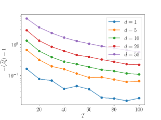
Figure 2. Effect of dimensionality on mean of (inferred) $\widehat{A}^{i}_{i}$ ($i$ not summed) when $-\mathbf{A}=\mathbf{D}=\mathbf{C}=\mathds{1}$.

For the second moment of $\widehat{\mathbf{A}}$, we need to evaluate the expectation:

(51) $$\left\langle{\left({\frac{1}{T}\int_{0}^{T}\mathrm{d}\tau\,\dot{x}^{i}(\tau)x^{j}(\tau)}\right)\sum_{m=0}^{\infty}(-1)^{m}[(\Delta\widehat{\mathbf{C}}(T))^{m}]^{kl}\left({\frac{1}{T}\int_{0}^{T}\mathrm{d}\tau^{\prime}\,\dot{x}^{i^{\prime}}(\tau^{\prime})x^{j^{\prime}}(\tau^{\prime})}\right)\sum_{n=0}^{\infty}(-1)^{n}[(\Delta\widehat{\mathbf{C}}(T))^{n}]^{k^{\prime}l^{\prime}}}\right\rangle.$$

The $m=n=0$ term is simply $\delta^{ij}\delta^{i^{\prime}j^{\prime}}$. For the $m+n=1$ terms, we need to evaluate:

(52) $$\frac{1}{T^{3}}\int_{0}^{T}\mathrm{d}\tau\int_{0}^{T}\mathrm{d}\tau^{\prime}\int_{0}^{T}\mathrm{d}\upsilon\,\langle\dot{x}^{i}(\tau)x^{j}(\tau)\dot{x}^{i^{\prime}}(\tau^{\prime})x^{j^{\prime}}(\tau^{\prime})(x^{k}(\upsilon)x^{l}(\upsilon)-\delta^{kl})\rangle=\frac{1}{T^{3}}\int_{0}^{T}\mathrm{d}\tau\int_{0}^{T}\mathrm{d}\tau^{\prime}\int_{0}^{T}\mathrm{d}\upsilon$$

$$\quad\Big{[}{\langle\dot{x}^{i}(\tau)x^{j}(\tau)\rangle(\langle\dot{x}^{i^{\prime}}(\tau^{\prime})x^{k}(\upsilon)\rangle\langle x^{j^{\prime}}(\tau^{\prime})x^{l}(\upsilon)\rangle+\langle\dot{x}^{i^{\prime}}(\tau^{\prime})x^{l}(\upsilon)\rangle\langle x^{j^{\prime}}(\tau^{\prime})x^{k}(\upsilon)\rangle)}\Big{.}$$

$$\qquad{}+\langle\dot{x}^{i^{\prime}}(\tau^{\prime})x^{j^{\prime}}(\tau^{\prime})\rangle(\langle\dot{x}^{i}(\tau)x^{k}(\upsilon)\rangle\langle x^{j}(\tau)x^{l}(\upsilon)\rangle+\langle\dot{x}^{i}(\tau)x^{l}(\upsilon)\rangle\langle x^{j}(\tau)x^{k}(\upsilon)\rangle)$$

$$\qquad{}+\langle\dot{x}^{i}(\tau)\dot{x}^{i^{\prime}}(\tau^{\prime})\rangle(\langle x^{j}(\tau)x^{k}(\upsilon)\rangle\langle x^{j^{\prime}}(\tau^{\prime})x^{l}(\upsilon)\rangle+\langle x^{j}(\tau)x^{l}(\upsilon)\rangle\langle x^{j^{\prime}}(\tau^{\prime})x^{k}(\upsilon)\rangle)$$

$$\qquad{}+\langle\dot{x}^{i}(\tau)x^{j^{\prime}}(\tau^{\prime})\rangle(\langle x^{j}(\tau)x^{k}(\upsilon)\rangle\langle\dot{x}^{i^{\prime}}(\tau^{\prime})x^{l}(\upsilon)\rangle+\langle x^{j}(\tau)x^{l}(\upsilon)\rangle\langle\dot{x}^{i^{\prime}}(\tau^{\prime})x^{k}(\upsilon)\rangle)$$

$$\qquad{}+\langle\dot{x}^{i}(\tau)x^{k}(\upsilon)\rangle(\langle x^{j}(\tau)\dot{x}^{i^{\prime}}(\tau^{\prime})\rangle\langle x^{j^{\prime}}(\tau^{\prime})x^{l}(\upsilon)\rangle+\langle x^{j}(\tau)x^{j^{\prime}}(\tau^{\prime})\rangle\langle\dot{x}^{i^{\prime}}(\tau^{\prime})x^{l}(\upsilon)\rangle)$$

$$\Big{.}{\qquad{}+\langle\dot{x}^{i}(\tau)x^{l}(\upsilon)\rangle(\langle x^{j}(\tau)\dot{x}^{i^{\prime}}(\tau^{\prime})\rangle\langle x^{j^{\prime}}(\tau^{\prime})x^{k}(\upsilon)\rangle+\langle x^{j}(\tau)x^{j^{\prime}}(\tau^{\prime})\rangle\langle\dot{x}^{i^{\prime}}(\tau^{\prime})x^{k}(\upsilon)\rangle)}\Big{]}.$$

The integrals of the first two lines vanish, and the remaining lines have integral $\mathcal{O}(T)$ (before dividing by $T^{3}$). For the $m+n=2$ terms, we have:

(53) $$\frac{1}{T^{4}}\int_{0}^{T}\mathrm{d}\tau\int_{0}^{T}\mathrm{d}\tau^{\prime}\int_{0}^{T}\mathrm{d}\upsilon\int_{0}^{T}\mathrm{d}\upsilon^{\prime}\,\langle\dot{x}^{i}(\tau)x^{j}(\tau)\dot{x}^{i^{\prime}}(\tau^{\prime})x^{j^{\prime}}(\tau^{\prime})(x^{k}(\upsilon)x^{l}(\upsilon)-\delta^{kl})(x^{k^{\prime}}(\upsilon^{\prime})x^{l^{\prime}}(\upsilon^{\prime})-\delta^{k^{\prime}l^{\prime}})\rangle$$

$$\quad{}=\frac{1}{T^{4}}\int_{0}^{T}\mathrm{d}\tau\int_{0}^{T}\mathrm{d}\tau^{\prime}\int_{0}^{T}\mathrm{d}\upsilon\int_{0}^{T}\mathrm{d}\upsilon^{\prime}\,\langle\dot{x}^{i}(\tau)x^{j}(\tau)\rangle\langle\dot{x}^{i^{\prime}}(\tau^{\prime})x^{j^{\prime}}(\tau^{\prime})\rangle$$

$$\qquad{}\times(\langle x^{k}(\upsilon)x^{k^{\prime}}(\upsilon^{\prime})\rangle\langle x^{l}(\upsilon)x^{l^{\prime}}(\upsilon^{\prime})\rangle+\langle x^{k}(\upsilon)x^{l^{\prime}}(\upsilon^{\prime})\rangle\langle x^{l}(\upsilon)x^{k^{\prime}}(\upsilon^{\prime})\rangle)+\mathcal{O}\left({\frac{1}{T^{2}}}\right)$$

$$\quad{}\approx\frac{\delta^{ij}\delta^{i^{\prime}j^{\prime}}(\delta^{kk^{\prime}}\delta^{ll^{\prime}}+\delta^{kl^{\prime}}\delta^{lk^{\prime}})}{T},\quad T\gg\frac{1}{2}.$$

This gives:

(54) $$\langle\widehat{A}(T)^{i}_{j}\widehat{A}(T)^{i^{\prime}}_{j^{\prime}}\rangle-\langle\widehat{A}(T)^{i}_{j}\rangle\langle\widehat{A}(T)^{i^{\prime}}_{j^{\prime}}\rangle\approx\frac{\delta^{ii^{\prime}}\delta^{jj^{\prime}}+\delta^{ij^{\prime}}\delta^{ji^{\prime}}}{T}.$$

Perhaps surprisingly, there is no $d$-dependence to leading order in $T^{-1}$ (Fig. 3). This means that it is possible for the bias to dominate the variance. The $d$-dependence in the variance presumably occurs at higher order, but we do not bother to calculate it.

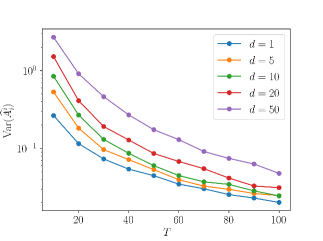
Figure 3. Effect of dimensionality on variance of (inferred) $\widehat{A}^{i}_{i}$ ($i$ not summed) when $-\mathbf{A}=\mathbf{D}=\mathbf{C}=\mathds{1}$.

Finally, we can calculate the covariance of the estimated drift:

(55) $$\langle\widehat{A}^{i}_{k}\widehat{A}^{j}_{l}\widehat{C}^{kl}\rangle=\frac{1}{T^{2}}\left\langle\left({\int_{0}^{T}\mathrm{d}\tau\,\dot{x}^{i}(\tau)x^{k}(\tau)}\right)\left({\int_{0}^{T}\mathrm{d}\tau^{\prime}\,\dot{x}^{j}(\tau^{\prime})x^{l}(\tau^{\prime})}\right)\sum_{n=0}^{\infty}[(\Delta\widehat{\mathbf{C}}(T))^{n}]^{kl}\right\rangle\approx\left({1+\frac{2d}{T}}\right)\delta^{ij},$$

which is an overestimate (Fig. 4).

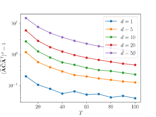
Figure 4. Effect of dimensionality on variance of inferred drift ($\widehat{A}^{i}_{k}\widehat{A}^{i}_{l}\widehat{C}^{kl}$, $i$ not summed) when $-\mathbf{A}=\mathbf{D}=\mathbf{C}=\mathds{1}$.

3. Integrated variables

3.1. Preliminaries: Definition, covariance functions, and detailed balance

In the statistical literature, the term “integrated variable” in a stochastic process refers to a variable with no stationary distribution, but whose increments, or increments of increments, etc., do possess a stationary distribution. Here, we focus on variables integrated of order one, i.e., variables whose increments possess a stationary distribution. Such variables can be used to model e.g. the position and orientation of a particle in a homogeneous, isotropic medium. The dynamics of these variables may depend on degrees of freedom represented by variables possessing a stationary distribution. For linear dynamics, this type of system is modeled as:

(56) $$\dot{\mathbf{x}} =\mathbf{A}\mathbf{x}+\boldsymbol{\xi}^{\mathbf{x}},$$

(57) $$\dot{y} =\boldsymbol{\alpha}^{\mathsf{T}}\mathbf{x}+\xi^{y},$$

(58) $$\langle\boldsymbol{\xi}^{\mathbf{x}}(t)\boldsymbol{\xi}^{\mathbf{x}}(t^{\prime})^{\mathsf{T}}\rangle =2\mathbf{D}^{\mathbf{x}\mathbf{x}}\delta(t-t^{\prime}),$$

(59) $$\langle\boldsymbol{\xi}^{\mathbf{x}}(t)\xi^{y}(t^{\prime})\rangle =2\mathbf{D}^{\mathbf{x}y}\delta(t-t^{\prime}),$$

(60) $$\langle\xi^{y}(t)\xi^{y}(t^{\prime})\rangle =2D^{yy}\delta(t-t^{\prime}).$$

where a possible additive constant in $\dot{y}$ has been omitted. In this case, the angular momentum is defined as:

(61) $$\mathbf{L}(\mathbf{x},y):=\lim_{\tau\to 0}\frac{\langle(\mathbf{x}(0)+\mathbf{x}(\tau))(y(\tau)-y(0))\rangle}{\tau}$$

which, in this model, evaluates to:

(62) $$\mathbf{L}(\mathbf{x},y)=2\langle\mathbf{x}\dot{y}\rangle+\left\langle{\frac{\mathrm{d}[\mathbf{x},y](t)}{\mathrm{d}t}}\right\rangle=2\mathbf{C}\boldsymbol{\alpha}+2\mathbf{D}^{\mathbf{x}y}.$$

The condition for detailed balance is $\mathbf{L}(\mathbf{x},y)=\mathbf{0}$ and $L(x^{i},x^{j})=0$ for all $i,j$.

To calculate covariance functions, it is useful to switch to a new variable:

(63) $$z:=y-\boldsymbol{\alpha}^{\mathsf{T}}\mathbf{A}^{-1}\mathbf{x},$$

so that $z$ obeys

(64) $$\dot{z}=\xi^{z},\quad\langle\xi^{z}(t)\rangle=0,\quad\langle\boldsymbol{\xi}^{\mathbf{x}}(t)\xi^{z}(t^{\prime})\rangle=2\mathbf{D}^{\mathbf{x}z}\delta(t-t^{\prime}),\quad\langle\xi^{z}(t)\xi^{z}(t^{\prime})\rangle=2D^{zz}\delta(t-t^{\prime}).$$

The transformed diffusion coefficients are:

(65) $$\mathbf{D}^{\mathbf{x}z} =\mathbf{D}^{\mathbf{x}y}-\mathbf{D}^{\mathbf{x}\mathbf{x}}(\mathbf{A}^{-1})^{\mathsf{T}}\boldsymbol{\alpha},$$

(66) $$D^{zz} =D^{yy}-2\boldsymbol{\alpha}^{\mathsf{T}}\mathbf{A}^{-1}\mathbf{D}^{\mathbf{x}y}+\boldsymbol{\alpha}^{\mathsf{T}}\mathbf{A}^{-1}\mathbf{D}^{\mathbf{x}\mathbf{x}}(\mathbf{A}^{-1})^{\mathsf{T}}\boldsymbol{\alpha}.$$

If detailed balance is satisfied for $\mathbf{x}$, then $\mathbf{D}^{\mathbf{x}\mathbf{x}}(\mathbf{A}^{-1})^{\mathsf{T}}=-\mathbf{C}$ and $\mathbf{L}(\mathbf{x},z)=\mathbf{L}(\mathbf{x},y)$. Moreover, the detailed balance condition for $z$ simply becomes $\mathbf{D}^{\mathbf{x}z}=\mathbf{0}$.

There are two kinds of covariance functions that can be evaluated. One is the forward-difference covariance function, which for $z$ evaluates to zero:

(67) $$\langle\mathbf{x}(0)(z(\tau)-z(0))\rangle=\mathbf{0},$$

where again $\tau\geq 0$ is (always) assumed. The backward-difference covariance function satisfies the equation:

(68) $$\frac{\mathrm{d}}{\mathrm{d}\tau}\langle\mathbf{x}(\tau)(z(\tau)-z(0))\rangle=\mathbf{A}\langle\mathbf{x}(\tau)(z(\tau)-z(0))\rangle+2\mathbf{D}^{\mathbf{x}z},$$

which has solution

(69) $$\langle\mathbf{x}(\tau)(z(\tau)-z(0))\rangle=2\mathbf{A}^{-1}\left({e^{\mathbf{A}\tau}-\mathds{1}}\right)\mathbf{D}^{\mathbf{x}z}.$$

We also have:

(70) $$\langle(z(\tau)-z(0))^{2}\rangle=2D^{zz}\tau.$$

Note that in the case where $\mathbf{x}$ is one-dimensional, the stochastic rotation frequency always vanishes because of a zero relaxation rate, but the entropy production does not vanish if detailed balance is broken.

To characterize the coupling between $\mathbf{x}$ and $y$, instead of $\boldsymbol{\alpha}$ and $\mathbf{D}^{\mathbf{x}y}$, we may prefer to use $\mathbf{L}(\mathbf{x},y)$ and $\mathbf{D}^{\mathbf{x}y}$. Here, we consider $\mathbf{L}(y,\mathbf{x}):=-\mathbf{L}(\mathbf{x},y)$ and use the same criterion as in the previous section to judge significance of angular momenta.

Between two integrated variables, there is no additional quantity governing break of detailed balance. Thus the angular momentum between them is considered to be 0, assuming that dynamics do not depend in any way on the values of those variables—in particular, not any combination of them.

3.2. Quantitative significance of the deterministic contribution

The next question we wish to consider is that of quantitative significance. How do we judge whether or not the deterministic contribution $\boldsymbol{\alpha}^{\mathsf{T}}\mathbf{x}$ to $y$ is significant? And how do we compare whether a fitted model is a good match to experimental data, at least to linear order? This question has been addressed in the case of the usual stationary variables: compare the values of the experimentally measured covariance functions to the theoretical model prediction, and if the difference is small compared to $\mathbf{C}$, it is declared a good fit. However, we cannot proceed in an analogous way because the measured quantities are differences $y(\tau)-y(0)$ whose expectations scale as $\tau^{1}$ whereas root-mean-square values $\langle(y(\tau)-y(0))^{2}\rangle^{1/2}$ scale as $\tau^{1/2}$. Hence, they are not comparable.

We specialize to the case where $\mathbf{x}$ is one-dimensional, i.e.:

(71) $$\dot{x} =-\lambda x+\xi^{x},$$

$$\dot{y} =\alpha x+\xi^{y},$$

where $\lambda>0$. The dimensionless combination involving $\alpha$ is $(\alpha/\lambda)\sqrt{D^{xx}/D^{yy}}$. We will explicitly arrive at this quantity by studying the function $\langle(y(\tau)-y(0))^{2}\rangle$. We introduce as before the variable $z$, with:

(72) $$z :=y+\frac{\alpha}{\lambda}x,$$

(73) $$D^{xz} =D^{xy}+\frac{\alpha}{\lambda}D^{xx},$$

(74) $$D^{zz} =D^{yy}+2\frac{\alpha}{\lambda}D^{xy}+\left({\frac{\alpha}{\lambda}}\right)^{2}D^{xx}.$$

From the covariance function above, we obtain:

(75) $$\langle(y(\tau)-y(0))^{2}\rangle=2D^{yy}\tau+2\frac{\alpha}{\lambda}\left({\frac{\alpha}{\lambda}D^{xx}+2D^{xy}}\right)\left({\tau-\frac{1-e^{-\lambda\tau}}{\lambda}}\right).$$

We see that depending on $D^{xy}$, the value can be either increased or decreased relative to that due to the deterministic ($\alpha$) or stochastic ($D^{yy}$) contributions alone. Nevertheless, some bounds can be established by using $\left|{D^{xy}}\right|\leq\sqrt{D^{xx}D^{yy}}$. By minimizing with respect to $\alpha$ while keeping $D^{yy}$ fixed, we get:

(76) $$\langle(y(\tau)-y(0))^{2}\rangle\geq 2D^{yy}\frac{1-e^{-\lambda\tau}}{\lambda}.$$

On the other hand, by minimizing with respect to $D^{yy}$ while keeping $\alpha$ fixed, we have

(77) $$\langle(y(\tau)-y(0))^{2}\rangle\geq 2\left({\frac{\alpha}{\lambda}}\right)^{2}D^{xx}\left({1-\frac{1-e^{-\lambda\tau}}{\lambda\tau}}\right)\frac{1-e^{-\lambda\tau}}{\lambda}.$$

Notice that both of these bounds stay finite as $\tau\to\infty$. The reason for this is that the $\tau\to\infty$ behavior of $\langle(y(\tau)-y(0))^{2}\rangle$ is given by $2D^{zz}\tau$ if $D^{zz}>0$, and $D^{zz}$ can be made arbitrarily small for any particular choice of either $\alpha$ and $D^{yy}$ (but not both simultaneously). Comparing these two bounds, we see that the relevant comparison is between $(\alpha/\lambda)\sqrt{D^{xx}}$ and $\sqrt{D^{yy}}$. Indeed, if $(|\alpha|/\lambda)\sqrt{D^{xx}}\ll\sqrt{D^{yy}}$, then the contribution of $D^{yy}$ to $\langle(y(\tau)-y(0))^{2}\rangle$ is dominant. On the other hand, if $(|\alpha|/\lambda)\sqrt{D^{xx}}\gg\sqrt{D^{yy}}$, then for long times $\tau\gg 1/\lambda$, the contribution of $\alpha$ to $\langle(y(\tau)-y(0))^{2}\rangle$ is dominant.

For multidimensional $\mathbf{x}$, we may compare the square roots of the quadratic variation of the two terms in Eq. (63).

3.3. Comparison of experimental data with theoretical predictions

To compare experimentally measured covariance functions to theoretical predictions, we can again normalize by the diffusion matrix. We may consider coordinates in which $\mathbf{D}=\mathds{1}$ and compare the experimental and theoretical values of $\langle\dot{\mathbf{x}}(\tau)\mathbf{x}(0)^{\mathsf{T}}\rangle$. Or, for a coordinate-independent description, similarly to the case of stationary variables, we may decompose the deviation of experimental to theoretical $\langle\dot{\mathbf{x}}(\tau)\mathbf{x}(0)^{\mathsf{T}}\rangle$ into symmetric and antisymmetric parts, multiply on the right by $\mathbf{D}^{-1}$ and inspect the eigenvalues and compare them to unity. In terms of “ensemble variance”, this amounts to:

(78) $$\Delta_{\textrm{exp\textendash theo}}\langle\dot{x}^{i}(\tau)x^{j}(0)\rangle\Delta_{\textrm{exp\textendash theo}}\langle\dot{x}^{i^{\prime}}(\tau)x^{j^{\prime}}(0)\rangle\sim D^{ii^{\prime}}D^{jj^{\prime}},$$

where $\Delta_{\textrm{exp\textendash theo}}$ denotes the deviation of experimental to theoretical values. As mentioned for the angular momentum, if the time-step is not small, then on the r.h.s. of the above, it may be suitable to use discrete-time estimators of the diffusion. In case the eigenvalues of $\mathbf{H}$ exceed unity, the eigenvalues need to be compared to these instead, not just for the antisymmetric part but also for the symmetric part. We may illustrate this by way of two-dimensional linear Gaussian dynamics with complex conjugate eigenvalues and $D^{xx}=D^{yy}$, $D^{xy}=0$, in which case:

(79) $$(\langle\dot{\mathbf{x}}(\tau)\mathbf{x}(0)^{\mathsf{T}}\rangle+\langle\mathbf{x}(0)\dot{\mathbf{x}}(\tau)^{\mathsf{T}}\rangle)(2\mathbf{D})^{-1}=e^{-\lambda\tau}\left({-\cos(\omega\tau)-\frac{\omega}{\lambda}\sin(\omega\tau)}\right)\mathds{1}.$$

Thus if $\omega/\lambda\gg 1$, deviation of experimental to theoretical values could be amplified by this factor. Now, we need to extend the notion of $\langle\dot{\mathbf{x}}(\tau)\mathbf{x}(0)^{\mathsf{T}}\rangle$ to integrated variables. We easily make the identification $\text{``$\langle\dot{\mathbf{x}}(\tau)y(0)\rangle$''}=-\langle\mathbf{x}(\tau)\dot{y}(0)\rangle$ for $\tau>0$. (For $\tau=0$, the time-derivative $\dot{y}(0)$ is interpreted in the anti-Itô sense.) For a pair of integrated variables $y$ and $z$ (not the same $z$ as in Eq. (63)), we manipulate the terms in the following equation, similarly to Eq. (5):

(80) $$2D^{yz}=\lim_{\tau\to 0}\frac{\langle(y(\tau)-y(0))(z(\tau)-z(0))\rangle}{\tau}=\text{``$\langle-\dot{y}z-y\dot{z}\rangle$''}.$$

Since there is no angular momentum between $y$ and $z$, we assign $\dot{y}z$ and $y\dot{z}$ the same (fictional) value, $-D^{yz}$. For non-zero time lags, we integrate:

(81) $$\text{``$\langle\dot{y}(\tau)z(0)\rangle$''}=\text{``$\langle\dot{y}(0)z(0)\rangle$''}-\int_{0^{+}}^{\tau}\mathrm{d}\tau^{\prime}\,\langle\dot{y}(\tau^{\prime})\dot{z}(0)\rangle.$$

As an example, for a single (integrated) variable the quantity in Eq. (81) approaches as $\tau\to\infty$ the negative of the long-time diffusivity, to be compared to the short-time diffusivity.

4. Third-order properties

So far, we have dealt with linear Gaussian systems. These are characterized by the quantities $\mathbf{A}$ and $\mathbf{D}$ which give rise to the second-order moments $\langle\mathbf{x}\mathbf{x}^{\mathsf{T}}\rangle$ and $\langle\dot{\mathbf{x}}\mathbf{x}^{\mathsf{T}}\rangle$. To address the possibility of third-order moments, we may consider additional terms in the model:

(82) $$\langle\dot{x}^{i}(t)\mid\mathbf{x}(t)\rangle =A^{i}_{j}x^{j}+a^{i}_{jk}(x^{j}x^{k}-C^{jk})$$

(83) $$\left\langle\frac{\mathrm{d}[x^{i},x^{j}](t)}{\mathrm{d}t}\mid\mathbf{x}(t)\right\rangle =2D^{ij}+2b^{ij}_{k}x^{k}$$

where we have suppressed $t$-dependence, and Einstein summation notation is used. Neither addition to the model can stand on its own: in general, $a^{i}_{jk}$ by itself leads to divergences of $\mathbf{x}\to\infty$, and $b^{ij}_{k}$ by itself renders $\langle\mathrm{d}[x^{i},x^{j}]/\mathrm{d}t\mid\mathbf{x}(t)\rangle$ not positive semidefinite. A third possible contribution,

(84) $$\lim_{\tau\to 0}\frac{\langle(x^{i}(\tau)-x^{i}(0))(x^{j}(\tau)-x^{j}(0))(x^{k}(\tau)-x^{k}(0))\rangle}{\tau}=0,$$

vanishes in the case where $\mathbf{x}$ has continuous paths. In such a situation, the probability density evolution satisfies a Fokker–Planck equation [3], leading to vanishing of the “cubic variation”. This gives a relation between the angular momenta, as:

(85) $$L(x^{i}x^{j},x^{k})+L(x^{j}x^{k},x^{i})+L(x^{k}x^{i},x^{j})=0.$$

This may also be understood by taking the time-derivative of (the time-independent quantity) $\langle x^{i}x^{j}x^{k}\rangle$ and interpreting in the Stratonovich sense.

The angular momenta are related to probability currents. We start with the Fokker–Planck equation:

(86) $$\frac{\partial}{\partial t}p(\mathbf{x},t)=-\frac{\partial}{\partial x^{i}}[\mathcal{A}^{i}(\mathbf{x})p(\mathbf{x},t)]+\frac{1}{2}\frac{\partial^{2}}{\partial x^{i}\partial x^{j}}[\mathcal{B}^{ij}(\mathbf{x})p(\mathbf{x},t)],$$

for which the probability current density $\mathbf{J}(\mathbf{x})$ reads [3]:

(87) $$J^{i}(\mathbf{x})=\mathcal{A}^{i}(\mathbf{x})p(\mathbf{x})-\frac{1}{2}\partial_{j}[\mathcal{B}^{ij}(\mathbf{x})p(\mathbf{x})],$$

where $p(\mathbf{x})$ is the stationary distribution. Multiplying by an arbitrary function $f(\mathbf{x})$ and integrating, we get:

(88) $$\int\mathrm{d}\mathbf{x}\,J^{i}(\mathbf{x})f(\mathbf{x}) =\langle\mathcal{A}^{i}(\mathbf{x})f(\mathbf{x})\rangle+\frac{1}{2}\langle\mathcal{B}^{ij}(\mathbf{x})\partial_{j}f(\mathbf{x})\rangle$$

$$=\langle f(\mathbf{x})\dot{x}^{i}\rangle+\frac{1}{2}\left\langle\frac{\mathrm{d}[f(\mathbf{x}),x^{i}](t)}{\mathrm{d}t}\right\rangle$$

$$=\langle f(\mathbf{x})\circ\dot{x}^{i}\rangle$$

$$=\frac{1}{2}L(f(\mathbf{x}),x^{i}).$$

Thus $L(x^{i}x^{j},x^{k})$ gives complete information about probability currents to “third order” (counting two orders for quadratic $f(\mathbf{x})$, and one order for $x^{i}$).

We can define other quantities that are odd under time reversal:

(89) $$\widetilde{L}(x^{i},x^{j},x^{k}):=\lim_{\tau\to 0}\frac{\langle x^{i}(\tau/2)(x^{j}(0)x^{k}(\tau)-x^{j}(\tau)x^{k}(0))\rangle}{\tau}.$$

We can use an Itô–Taylor expansion [10] to compute this as:

(90) $$\widetilde{L}(x^{i},x^{j},x^{k})=\langle x^{i}(x^{j}\mathcal{A}^{k}(\mathbf{x})-\mathcal{A}^{j}(\mathbf{x})x^{k})\rangle+\frac{\langle\mathcal{B}^{ik}(\mathbf{x})x^{j}-\mathcal{B}^{ij}(\mathbf{x})x^{k}\rangle}{2}=\frac{L(x^{i}x^{j},x^{k})-L(x^{i}x^{k},x^{j})}{2}$$

We can invert this relationship to give $L$ in terms of $\widetilde{L}$:

(91) $$L(x^{i}x^{j},x^{k})=\frac{2}{3}\left[{\widetilde{L}(x^{i},x^{j},x^{k})+\widetilde{L}(x^{j},x^{i},x^{k})}\right].$$

Thus $\widetilde{L}$ also gives complete information about time-reversal asymmetry to third order. This will become useful when we consider underdamped processes. Like $L$, it satisfies the relation:

(92) $$\widetilde{L}(x^{i},x^{j},x^{k})+\widetilde{L}(x^{j},x^{k},x^{i})+\widetilde{L}(x^{k},x^{i},x^{j})=0.$$

Now, we address the case of integrated variables. The angular momentum involving $y$ is again defined by Eq. (61) and the requirement for detailed balance is $L(x^{i}x^{j},y)=0$. We can compute:

(93) $$L(x^{i}x^{j},y)=2\langle x^{i}x^{j}\mathcal{A}^{y}(\mathbf{x})\rangle+\langle x^{i}\mathcal{B}^{jy}(\mathbf{x})\rangle+\langle x^{j}\mathcal{B}^{iy}(\mathbf{x})\rangle.$$

It can be shown that:

(94) $$\lim_{\tau\to 0}\frac{\langle(x^{i}(0)x^{j}(\tau)+x^{i}(\tau)x^{j}(0))(y(\tau)-y(0))\rangle}{\tau}=\lim_{\tau\to 0}\frac{\langle x^{i}(\tau/2)(x^{j}(0)+x^{j}(\tau))(y(\tau)-y(0))\rangle}{\tau}=L(x^{i}x^{j},y).$$

For inhomogeneous diffusion, we have from Eq. (84):

(95) $$\lim_{\tau\to 0}\frac{\langle x^{i}(\tau)(x^{j}(\tau)-x^{j}(0))(x^{k}(\tau)-x^{k}(0))\rangle}{\tau}=\lim_{\tau\to 0}\frac{\langle x^{i}(0)(x^{j}(\tau)-x^{j}(0))(x^{k}(\tau)-x^{k}(0))\rangle}{\tau}.$$

5. Inhomogeneous diffusion

In this section, we shall restrict ourselves to the case where $\langle\dot{\mathbf{x}}\mid\mathbf{x}\rangle$ is linear. In addition to being easier to deal with, in the case of weak nonlinearity, coordinates can be chosen via Koopman eigenfunctions [16, 17] to transform the system into this form, as will be done in the next section. Additional terms in inhomogeneous diffusion are assumed to be small.

Our first task is the compute the third moments $\langle x^{i}x^{j}x^{k}\rangle$. In analogy with the derivation of the Lyapunov equation, we have:

(96) $$0=\langle(\mathbf{A}\mathbf{x})^{i}x^{j}x^{k}\rangle+\langle x^{i}(\mathbf{A}\mathbf{x})^{j}x^{k}\rangle+\langle x^{i}x^{j}(\mathbf{A}\mathbf{x})^{k}\rangle+2b^{ij}_{l}C^{kl}+2b^{ik}_{l}C^{jl}+2b^{jk}_{l}C^{il},$$

which has solution

(97) $$\langle x^{i}x^{j}x^{k}\rangle=-\left[{(\mathbf{A}\otimes\mathds{1}\otimes\mathds{1}+\mathds{1}\otimes\mathbf{A}\otimes\mathds{1}+\mathds{1}\otimes\mathds{1}\otimes\mathbf{A})^{-1}}\right]^{ijk}_{i^{\prime}j^{\prime}k^{\prime}}\left({2b^{i^{\prime}j^{\prime}}_{l}C^{k^{\prime}l}+2b^{i^{\prime}k^{\prime}}_{l}C^{j^{\prime}l}+2b^{j^{\prime}k^{\prime}}_{l}C^{i^{\prime}l}}\right).$$

The second task is to compute covariance functions. In the current model, $\langle\mathbf{x}(\tau)\mid\mathbf{x}(0)\rangle=e^{\mathbf{A}\tau}\mathbf{x}(0)$, so:

(98) $$\langle x^{i}(\tau)x^{j}(0)x^{k}(0)\rangle=(e^{\mathbf{A}\tau})^{i}_{i^{\prime}}\langle x^{i^{\prime}}x^{j}x^{k}\rangle.$$

Now, the function $\langle x^{i}(\tau)x^{j}(\tau)\mid\mathbf{x}(0)\rangle$ satisfies the equation:

(99) $$\frac{\mathrm{d}}{\mathrm{d}\tau}\langle x^{i}(\tau)x^{j}(\tau)\mid\mathbf{x}(0)\rangle =\langle(\mathbf{A}\mathbf{x})^{i}(\tau)x^{j}(\tau)\mid\mathbf{x}(0)\rangle+\langle x^{i}(\tau)(\mathbf{A}\mathbf{x})^{j}(\tau)\mid\mathbf{x}(0)\rangle$$

$$\quad{}+2D^{ij}+2b^{ij}_{k}(e^{\mathbf{A}\tau})^{k}_{k^{\prime}}x^{k^{\prime}}(0)$$

which has solution

(100) $$\langle x^{i}(\tau)x^{j}(\tau)\mid\mathbf{x}(0)\rangle=C^{ij}+(e^{\mathbf{A}\tau})^{i}_{i^{\prime}}(e^{\mathbf{A}\tau})^{j}_{j^{\prime}}\left({x^{i^{\prime}}(0)x^{j^{\prime}}(0)-C^{i^{\prime}j^{\prime}}}\right)$$

$$\qquad{}+2\left[{(\mathbf{A}\otimes\mathds{1}\otimes\mathds{1}+\mathds{1}\otimes\mathbf{A}\otimes\mathds{1}-\mathds{1}\otimes\mathds{1}\otimes\mathbf{A})^{-1}(e^{\mathbf{A}\tau}\otimes e^{\mathbf{A}\tau}\otimes\mathds{1}-\mathds{1}\otimes\mathds{1}\otimes e^{\mathbf{A}\tau})}\right]^{ijk}_{i^{\prime}j^{\prime}k^{\prime}}b^{i^{\prime}j^{\prime}}_{k}x^{k^{\prime}}(0).$$

The covariance function $\langle x^{i}(\tau)x^{j}(\tau)x^{k}(0)\rangle$ is then easily obtained.

The last task is to understand time-reversal asymmetry. We can easily compute the angular momenta:

(101) $$L(x^{i}x^{j},x^{k})=\langle x^{i}x^{j}(\mathbf{A}\mathbf{x})^{k}\rangle-\langle(\mathbf{A}\mathbf{x})^{i}x^{j}x^{k}\rangle-\langle x^{i}(\mathbf{A}\mathbf{x})^{j}x^{k}\rangle-2b^{ij}_{l}C^{kl}.$$

The question is, if this quantity is 0 for all $i,j,k$, are the covariance functions time-reversible? We see that we need the lower-order time-reversibility to hold, i.e., $\mathbf{A}\mathbf{C}=\mathbf{C}\mathbf{A}^{\mathsf{T}}$. Calling $\widetilde{\mathbf{A}}(\tau)$ the long quantity in square brackets in Eq. (100) involving $\mathbf{A}$, we have the covariance function:

(102) $$\langle x^{i}(\tau)x^{j}(\tau)x^{k}(0)\rangle=(e^{\mathbf{A}\tau})^{i}_{i^{\prime}}(e^{\mathbf{A}\tau})^{j}_{j^{\prime}}\langle x^{i^{\prime}}x^{j^{\prime}}x^{k}\rangle+2\widetilde{A}(\tau)^{ijl}_{i^{\prime}j^{\prime}k^{\prime}}b^{i^{\prime}j^{\prime}}_{l}C^{kk^{\prime}}.$$

Now from $\mathbf{A}\mathbf{C}=\mathbf{C}\mathbf{A}^{\mathsf{T}}$, we have:

(103) $$\widetilde{A}(\tau)^{ijl}_{i^{\prime}j^{\prime}k^{\prime}}C^{kk^{\prime}}=\widetilde{A}(\tau)^{ijk}_{i^{\prime}j^{\prime}k^{\prime}}C^{k^{\prime}l}.$$

Now in $\langle x^{i}(0)x^{j}(0)x^{k}(\tau)\rangle-\langle x^{i}(\tau)x^{j}(\tau)x^{k}(0)\rangle$ we can pull out a factor of $e^{\mathbf{A}\tau}\otimes e^{\mathbf{A}\tau}\otimes\mathds{1}-\mathds{1}\otimes\mathds{1}\otimes e^{\mathbf{A}\tau}$ and thus the condition for this quantity to be 0 for all $\tau$ and all $i,j,k$ reduces to that of $L(x^{i}x^{j},x^{k})=0$.

So far, we have understood how the quantities $b$ give rise to the quantities $\langle x^{i}x^{j}x^{k}\rangle$ and $L(x^{i}x^{j},x^{k})$. The remaining degree of freedom, $\langle x^{i}x^{j}\dot{x}^{k}\rangle$ is accounted for by nonlinearities, considered in the next section.

Now we turn to an example in two dimensions. Assume that there is a symmetry $y\to-y$, so that $\mathbf{A}=\operatorname{diag}(-\lambda_{x},-\lambda_{y})$ with $D^{xy}=0$ and $b^{xx}_{y}=b^{xy}_{x}=b^{yy}_{y}=0$. Then $\langle x^{2}\rangle=D^{xx}/\lambda_{x}$, $\langle y^{2}\rangle=D^{yy}/\lambda_{y}$, and

(104) $$\langle x^{3}\rangle =\frac{2b^{xx}_{x}\langle x^{2}\rangle}{\lambda_{x}},$$

(105) $$L(x^{2},x) =0,$$

(106) $$\langle xy^{2}\rangle =\frac{2b^{yy}_{x}\langle x^{2}\rangle+4b^{xy}_{y}\langle y^{2}\rangle}{\lambda_{x}+2\lambda_{y}},$$

(107) $$L(x,y^{2}) =\frac{4\lambda_{x}b^{yy}_{x}\langle x^{2}\rangle+4(\lambda_{x}-2\lambda_{y})b^{xy}_{y}\langle y^{2}\rangle}{\lambda_{x}+2\lambda_{y}},$$

(108) $$L(xy,y) =\frac{L(x,y^{2})}{2}.$$

We see that there is only one “mode of time-reversal asymmetry”, corresponding to $L(x,y^{2})$. An angular momentum $L(x,y^{2})>0$ represents probability current which is anticlockwise for $y>0$ and clockwise for $y<0$. We see that $b^{yy}_{x}$ contributes positively to $L(x,y^{2})$. However, the sign of the contribution due to $b^{xy}_{y}$ depends on the ratio $\lambda_{x}/\lambda_{y}$.

The question now arises: if $L(x,y^{2})=0$, is time-reversal symmetry truly satisfied? To answer this question, we investigate Eq. (88) where $i=x$ and $f(x,y)=y^{4}$. First, we write for the moment:

(109) $$0=\frac{\mathrm{d}}{\mathrm{d}t}\langle x(t)y(t)^{4}\rangle=(-\lambda_{x}-4\lambda_{y})\langle xy^{4}\rangle+8b^{xy}_{y}\langle y^{4}\rangle+12b^{yy}_{x}\langle x^{2}y^{2}\rangle.$$

Now treating the added term in the model as a perturbation, the fourth moments obey:

(110) $$\langle y^{4}\rangle =3\langle y^{2}\rangle+\mathcal{O}(b^{2})$$

(111) $$\langle x^{2}y^{2}\rangle =\langle x^{2}\rangle\langle y^{2}\rangle+\mathcal{O}(b^{2}).$$

Now we write the condition for detailed balance for this choice of $f$:

(112) $$-\lambda_{x}\langle xy^{4}\rangle=-4b^{xy}_{y}\langle y^{4}\rangle.$$

We see that the above is not generally satisfied, even to order $\mathcal{O}(b)$, when $L(x,y^{2})=0$. Thus $L(x,y^{2})=0$ is not a sufficient condition for detailed balance in the model; higher-order terms in $\mathbf{x}$ need to be included in the dynamics in order to truly satisfy detailed balance. However, this effect is absent from the third-order covariance functions.

Now, we address the case of integrated variables. Following the previous section, we assume such a variable $y$ obeys the law $\langle\dot{y}\mid\mathbf{x}\rangle=0$. We now use the model:

(113) $$\left\langle\frac{\mathrm{d}[x^{i},y](t)}{\mathrm{d}t}\mid\mathbf{x}(t)\right\rangle =2D^{iy}+2b^{iy}_{j}x^{j},$$

(114) $$\left\langle\frac{\mathrm{d}[y,y](t)}{\mathrm{d}t}\mid\mathbf{x}(t)\right\rangle =2D^{yy}+2b^{yy}_{i}x^{i}.$$

Then:

(115) $$L(x^{i}x^{j},y)=2b^{iy}_{k}C^{jk}+2b^{jy}_{k}C^{ik}.$$

We can solve for the covariance functions in the same manner as before. Therefore, we focus on the condition for detailed balance. As before, we have:

(116) $$\langle x^{i}(0)x^{j}(0)(y(\tau)-y(0))\rangle=0.$$

The following covariance function satisfies the equation:

(117) $$\frac{\mathrm{d}}{\mathrm{d}\tau}\langle x^{i}(\tau)x^{j}(\tau)(y(\tau)-y(0))\rangle =\langle(\mathbf{A}\mathbf{x})^{i}(\tau)x^{j}(\tau)(y(\tau)-y(0))\rangle+\langle x^{i}(\tau)(\mathbf{A}\mathbf{x})^{j}(\tau)(y(\tau)-y(0))\rangle$$

$$\qquad{}+2b^{ij}_{k}\langle x^{k}(\tau)(y(\tau)-y(0))\rangle+2b^{iy}_{k}C^{jk}+2b^{jy}_{k}C^{ik}.$$

We note that if $D^{ky}=0$ for $k$ stationary, which is a condition for detailed balance, then $\langle x^{k}(\tau)(y(\tau)-y(0))\rangle=0$. If in addition $2b^{iy}_{k}C^{jk}+2b^{jy}_{k}C^{ik}=0$, then $\langle x^{i}(\tau)x^{j}(\tau)(y(\tau)-y(0))\rangle=0$.

The other covariance function is of the form:

(118) $$\langle x^{i}(\tau)x^{j}(0)(y(\tau)-y(0))\rangle=2\left[{\lim_{\nu\to 1}(\nu\mathbf{A}\otimes\mathds{1}-\mathds{1}\otimes\mathbf{A})^{-1}(e^{\nu\mathbf{A}\tau}\otimes\mathds{1}-\mathds{1}\otimes e^{\mathbf{A}\tau})}\right]^{ik}_{i^{\prime}l}b^{i^{\prime}y}_{k}C^{jl}.$$

If $\mathbf{A}\mathbf{C}=\mathbf{C}\mathbf{A}^{\mathsf{T}}$, then calling $\widetilde{\mathbf{A}}(\tau)$ the long quantity in the square brackets involving $\mathbf{A}$:

(119) $$\widetilde{A}(\tau)^{ik}_{i^{\prime}l}C^{jl}=\widetilde{A}(\tau)^{ij}_{i^{\prime}l}C^{kl}.$$

If in addition $b^{iy}_{k}C^{jk}=-b^{jy}_{k}C^{ik}$, then we may write:

(120) $$\langle x^{i}(\tau)x^{j}(0)(y(\tau)-y(0))\rangle=-2\widetilde{A}(\tau)^{ij}_{i^{\prime}l}b^{ly}_{k}C^{i^{\prime}k}=-2\widetilde{A}(\tau)^{kj}_{i^{\prime}l}b^{ly}_{k}C^{ii^{\prime}}=-\langle x^{i}(0)x^{j}(\tau)(y(\tau)-y(0))\rangle$$

where we used $\widetilde{A}(\tau)^{ij}_{kl}=\widetilde{A}(\tau)^{ji}_{lk}$.

At this point, we introduce a second integrated variable $z$ obeying $\langle\dot{z}\mid\mathbf{x}\rangle=0$ as well as analogous laws as for $y$ with corresponding notation. The term $b^{yz}_{i}$ does not give rise to breaking detailed balance. However, detailed balance can still be broken to lower order in $\mathbf{x},y,z$ and as before, this will be reflected in the three-point covariance functions. Specifically, we can compute:

(121) $$\langle x^{i}(0)(y(\tau)-y(0))(z(\tau)-z(0))\rangle=2\left[{\mathbf{A}^{-1}(e^{\mathbf{A}\tau}-\mathds{1})}\right]^{j}_{k}b^{yz}_{j}C^{ik}.$$

We can write down the differential equation in the other direction:

(122) $$\frac{\mathrm{d}}{\mathrm{d}\tau}\langle x^{i}(\tau)(y(\tau)-y(0))(z(\tau)-z(0))\rangle =\langle(\mathbf{A}\mathbf{x})^{i}(y(\tau)-y(0))(z(\tau)-z(0))\rangle+2b^{iy}_{j}\langle x^{j}(\tau)(z(\tau)-z(0))\rangle$$

$$\qquad{}+2b^{iz}_{j}\langle x^{j}(\tau)(y(\tau)-y(0))\rangle+2b^{yz}_{j}C^{ij}.$$

We will again not solve this equation in full, but will simply assume $D^{iy}=D^{iz}=0$ for all stationary $i$, corresponding to detailed balance. Under this condition, the covariance function becomes:

(123) $$\langle x^{i}(\tau)(y(\tau)-y(0))(z(\tau)-z(0))\rangle=2\left[{\mathbf{A}^{-1}(e^{\mathbf{A}\tau}-\mathds{1})}\right]^{i}_{k}b^{yz}_{j}C^{jk}.$$

If $\mathbf{A}\mathbf{C}=\mathbf{C}\mathbf{A}^{\mathsf{T}}$, it is seen that the two covariance functions are equal.

6. Nonlinear drift

6.1. Preliminaries

Processes with nonlinear drift suffer from the fact that the determination of lower-order moments depends on higher-order moments. We first address the case in one dimension. We set the relaxation time and the diffusion coefficient to 1. Then to a first approximation, $\langle x^{2}\rangle=1$. As mentioned before, a quadratic function for $\langle\dot{x}\mid x\rangle$ gives rise to diverging $x$. Thus a cubic contribution is needed for stability. However, if this cubic contribution is too small, $x$ will no longer be localized around 0. We consider an “extreme” case where $\langle\dot{x}\mid x\rangle$ has a double zero. Such a case is attained by the function

(124) $$\langle\dot{x}\mid x\rangle=-x\left({\frac{ax}{2}-1}\right)^{2}=-x+ax^{2}-\frac{a^{2}}{4}x^{3},$$

showing that we only need the coefficient of $x^{3}$ to be $\mathcal{O}(a^{2})$ for the model to make sense, a result which could have been anticipated by symmetry. Thus, for small $a$, we can interpret the quadratic model for $\langle\dot{x}\mid x\rangle$ irrespective of any higher-order contributions. We also assume the linear model for inhomogeneous diffusion, noting similarly that in order for the diffusion function to be non-negative we can add a term $(b^{2}/4)x^{2}$, which is $\mathcal{O}(b^{2})$. Thus, to order $\mathcal{O}((a,b)^{2})$, our model is:

(125) $$\langle\dot{x}\mid x\rangle =-x+a(x^{2}-1),$$

(126) $$\left\langle\frac{\mathrm{d}[x,x](t)}{\mathrm{d}t}\mid x\right\rangle =2(1+bx).$$

6.2. One-dimensional case

Our first task is to compute the moments. We do this by introducing the probabilist’s Hermite polynomials ${He}_{n}(x)$ and calculating their time-derivatives using Itô’s lemma:

(127) $$\left\langle\frac{\mathrm{d}}{\mathrm{d}t}{He}_{n}(x)\mid x\right\rangle =-n{He}_{n}(x)+na\left[{{He}_{n+1}(x)+2(n-1){He}_{n-1}(x)+(n-1)(n-2){He}_{n-3}(x)}\right]$$

$$\qquad{}+n(n-1)b\left[{{He}_{n-1}(x)+(n-2){He}_{n-3}(x)}\right].$$

This gives rise to a system of equations for $\langle{He}_{n}(x)\rangle$, as:

(128) $$\begin{pmatrix}1&&&&&\\ &-1&a&&&\\ &2a+b&-1&a&&\\ 2(a+b)&&2(2a+b)&-1&a&\\ &6(a+b)&&3(2a+b)&-1&\ddots\\ &&\ddots&&\ddots&\ddots\end{pmatrix}\begin{pmatrix}\langle{He}_{0}(x)\rangle\\ \langle{He}_{1}(x)\rangle\\ \langle{He}_{2}(x)\rangle\\ \langle{He}_{3}(x)\rangle\\ \langle{He}_{4}(x)\rangle\\ \vdots\end{pmatrix}=\begin{pmatrix}1\\ 0\\ 0\\ 0\\ 0\\ \vdots\end{pmatrix}.$$

We solve this by truncation, which gives

(129) $$\langle x\rangle =a^{2}\mathcal{O}(a,b),$$

(130) $$\langle{He}_{2}(x)\rangle =a\mathcal{O}(a,b),$$

(131) $$\langle{He}_{3}(x)\rangle =2(a+b)+a\mathcal{O}((a,b)^{2}),$$

(132) $$|\langle{He}_{n}(x)\rangle| \leq\mathcal{O}((a,b)^{2}),\quad n\geq 4.$$

This is similar to an asymptotic expansion in that the above behavior holds as $a,b\to 0$ for any finite maximum degree $N$, but the solutions do not converge for fixed $a\neq 0$ as $N\to\infty$, as expected since trajectories obeying the Langevin equation diverge. Notice that the actual values of $\langle x\rangle$ and $\langle x^{2}\rangle$ differ from the “nominal” values of 0 and 1, respectively, used to construct the equation for the dynamics. We may understand this by rescaling $x$ and $t$ and attempting to set the mean and variance of $x$ to $\mu$ and $\nu$ respectively, obtaining:

(133) $$\langle\dot{x}\mid x\rangle =A\left\{{x-\mu+\frac{a}{\sqrt{D/A}}\left[{(x-\mu)^{2}-\nu}\right]}\right\},$$

(134) $$\left\langle\frac{\mathrm{d}[x,x]}{\mathrm{d}t}\mid x\right\rangle =2D\left[{1+b(x-\mu)}\right].$$

Apparently, there are 6 parameters ($A$, $D$, $a$, $b$, $\mu$, $\nu$); however, there are actually only 5 (quadratic drift has only 3 coefficients). Thus, if $\mu$ and $\nu>0$ are the actual mean and variance of $x$, then given these together with $D>0$ and $b$, the possible values of the pair $(A,a)$ must lie along a one-dimensional manifold. Thus in Eq. (82), $\mathbf{C}$ should be interpreted as a “nominal” value not necessarily corresponding to the actual covariance matrix. In particular, we will take it to be the value obeying the Lyapunov equation for the linear part of the dynamics (Eq. (3)).

Now we introduce the stochastic Koopman operator $\mathcal{K}$ [16, 17]. It is defined as an operator on functions of state space $f(\mathbf{x})$, as follows:

(135) $$(\mathcal{K}f)(\mathbf{x})=\left\langle\frac{\mathrm{d}f(\mathbf{x}(t))}{\mathrm{d}t}\mid\mathbf{x}(t)=\mathbf{x}\right\rangle.$$

The significance of the eigenfunctions of the stochastic Koopman operator (hereafter called “Koopman eigenfunctions”) is that their dynamics follows a linear law in expectation. Techniques and results for estimation of the Koopman operator are presented in [18, 19]. When $a=b=0$, the Koopman eigenfunctions are the probabilist’s Hermite polynomials ${He}_{n}(x)$ with eigenvalues $-n$. In the present case, the Koopman eigenfunctions $f_{n}(x)$ and the corresponding eigenvalues $\lambda_{n}$ are:

(136) $$f_{1}(x) =a^{2}\mathcal{O}(a,b){He}_{0}(x)+{He}_{1}(x)+(a+a^{2}\mathcal{O}(a,b)){He}_{2}(x)$$

$$\qquad{}+a^{2}\mathcal{O}(1){He}_{3}(x)+a^{3}\mathcal{O}(1){He}_{4}(x)+\cdots,$$

(137) $$\lambda_{1} =-1+a\mathcal{O}(a,b);$$

(138) $$f_{2}(x) =a\mathcal{O}(a,b){He}_{0}(x)+(-2(2a+b)+a^{2}\mathcal{O}(a,b)){He}_{1}(x)+{He}_{2}(x)$$

$$\qquad{}+(2a+a^{2}\mathcal{O}(a,b)){He}_{3}(x)+a^{2}\mathcal{O}(1){He}_{4}(x)+\cdots,$$

(139) $$\lambda_{2} =-2+a\mathcal{O}(a,b).$$

Now to calculate covariance functions, we use the linearity property of eigenfunctions:

(140) $$\langle f_{n}(x(\tau))g(x(0))\rangle=e^{\lambda_{n}\tau}\langle f_{n}(x(0))g(x(0))\rangle.$$

First, we apply this to $n=1$ and $g(x)=x$, leading to:

(141) $$\langle(x(\tau)+a{He}_{2}(x(\tau)))x(0)\rangle=e^{-\tau}\langle(x(0)+a{He}_{2}(x(0)))x(0)\rangle+a\mathcal{O}(a,b).$$

Now, just like the moments, $\langle{He}_{2}(x(\tau))x(0)\rangle=\mathcal{O}(a,b)$ and so

(142) $$\langle x(\tau)x(0)\rangle=e^{-\tau}+a\mathcal{O}(a,b),$$

where the quadratic correction could have been anticipated by symmetry. Thus the second-order covariance functions can be expected to be a poor proxy for nonlinearity.

Next, we would like the covariance function with $g(x)=x^{2}$. However, we need to use Isserlis’s theorem to calculate $\langle(x(\tau)^{2}-1)x(0)^{2}\rangle$ to zeroth-order in $a,b$. In fact, by symmetry, this has corrections of order only $\mathcal{O}((a,b)^{2})$, and we could show this explicitly by calculating $\langle f_{2}(x(\tau))f_{2}(x(0))\rangle$ (which we will not do). The result is:

(143) $$\langle x(\tau)x(0)^{2}\rangle=2(a+b)e^{-\tau}+2a(e^{-\tau}-e^{-2\tau})+a\mathcal{O}((a,b)^{2}).$$

Addressing the other covariance function, in one dimension this should be identical, but we calculate it again here. The eigenfunction $f_{2}(x(\tau))$ involves ${He}_{3}(x(\tau))$, but when multiplying by $x(0)$ and taking the expectation, it vanishes to zeroth order. Thus Isserlis’s theorem holds again to zeroth order. The result is:

(144) $$\langle x(\tau)^{2}x(0)\rangle=2(a+b)e^{-2\tau}-2(2a+b)(e^{-2\tau}-e^{-\tau})+a\mathcal{O}((a,b)^{2}),$$

which is indeed identical to Eq. (143).

We now present some numerical simulations to confirm the above results. We simulate a one-dimensional stochastic process where $\langle\dot{x}\mid x\rangle$ follows Eq. (124) with $x\to x+a$ and inhomogeneous diffusion $(1+bx/2)^{2}$. We use an Euler–Maruyama discretization with time-step $\Delta t=0.05$ and trajectory length $10^{6}$ time-units. Although corrections to the third-order covariance functions are only cubic order in $a,b$, they turn out to be quite large, as shown in Fig. 5 (the exception being when $a=0$). The second-order covariance function is also affected, although less so (Fig. 6), but the deviation is still larger than what one might expect for a quadratic correction. However, the deviations are limited to approximate multiplication by a constant, and thus nonlinearity cannot be effectively discerned from the second-order covariance functions, as expected. For larger values of $|a|$ ($\sim$ 0.3), the covariance functions are nowhere near the theoretically predicted values (not shown).

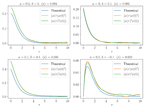
Figure 5. Third-order covariance functions.

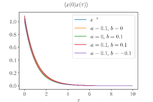
Figure 6. Second-order covariance functions.

6.3. Multidimensional case

Now we consider the multidimensional case, given by Eqs. (82)–(83). Without loss of generality, we assume $a^{i}_{jk}=a^{i}_{kj}$. We could expand functions in terms of multidimensional Hermite polynomials, defined as:

(145) $$x^{i},\quad x^{i}x^{j}-C^{ij},\quad x^{i}x^{j}x^{k}-C^{ij}x^{k}-C^{ik}x^{j}-C^{jk}x^{i},\quad\ldots.$$

We could use these to calculate multidimensional generalizations of the Koopman eigenfunctions satisfying $\langle\mathrm{d}\mathbf{f}(\mathbf{x}(t))/\mathrm{d}t\mid\mathbf{x}(t)\rangle=\mathbf{A}\mathbf{f}(\mathbf{x}(t))$ to transform into the case of the previous section ($a=0$). However, we opt for a more direct approach here and calculate covariance functions by means of differential equations, as in the previous sections. We must first calculate the third moments to order $\mathcal{O}(a,b)$:

(146) $$\langle x^{i}x^{j}x^{k}\rangle =-2\left[{(\mathbf{A}\otimes\mathds{1}\otimes\mathds{1}+\mathds{1}\otimes\mathbf{A}\otimes\mathds{1}+\mathds{1}\otimes\mathds{1}\otimes\mathbf{A})^{-1}}\right]^{ijk}_{i^{\prime}j^{\prime}k^{\prime}}$$

$$\qquad{}\times\left({a^{i^{\prime}}_{lm}C^{j^{\prime}l}C^{k^{\prime}m}+a^{j^{\prime}}_{lm}C^{i^{\prime}l}C^{k^{\prime}m}+a^{k^{\prime}}_{lm}C^{i^{\prime}l}C^{j^{\prime}m}+b^{i^{\prime}j^{\prime}}_{l}C^{k^{\prime}l}+b^{i^{\prime}k^{\prime}}_{l}C^{j^{\prime}l}+b^{j^{\prime}k^{\prime}}_{l}C^{i^{\prime}l}}\right)$$

$$\quad{}+a\mathcal{O}((a,b)^{2}).$$

For the covariance functions, we solve a differential equation, replacing fourth-order moments using Isserlis’s theorem, with $\mathcal{O}((a,b)^{2})$ corrections. Without going through the details of the calculations, we use again the quantity we called $\widetilde{\mathbf{A}}(\tau)$ (the long quantity in square brackets in Eq. (100)), and the result is:

(147) $$\langle x^{i}(0)x^{j}(0)x^{k}(\tau)\rangle =(e^{\mathbf{A}\tau})^{k}_{k^{\prime}}\langle x^{i}x^{j}x^{k^{\prime}}\rangle+2\widetilde{A}(\tau)^{i^{\prime}j^{\prime}k}_{lmk^{\prime}}a^{k^{\prime}}_{i^{\prime}j^{\prime}}C^{il}C^{jm}+a\mathcal{O}((a,b)^{2}),$$

$$\langle x^{i}(\tau)x^{j}(\tau)x^{k}(0)\rangle =(e^{\mathbf{A}\tau})^{i}_{i^{\prime}}(e^{\mathbf{A}\tau})^{j}_{j^{\prime}}\langle x^{i^{\prime}}x^{j^{\prime}}x^{k}\rangle+2\widetilde{A}(\tau)^{ijk^{\prime}}_{i^{\prime}j^{\prime}l}\left({b^{i^{\prime}j^{\prime}}_{k^{\prime}}+a^{i^{\prime}}_{k^{\prime}m}C^{j^{\prime}m}+a^{j^{\prime}}_{k^{\prime}m}C^{i^{\prime}m}}\right)C^{kl}$$

(148) $$\quad{}+a\mathcal{O}((a,b)^{2}).$$

As expected, we see that as in the case where $a=0$, the third-order covariance functions are symmetric (with $a\mathcal{O}((a,b)^{2})$ corrections) if $L(x^{i},x^{j})=0$ and $L(x^{i}x^{j},x^{k})=0$ for all $i,j,k$.

At this point, we note that by a similar calculation, if there are cubic terms in the drift or quadratic terms in the diffusivity, then the corrections to the second- and third-order covariance functions are quadratic in the coefficients deviating from a linear Gaussian model (written in terms of multidimensional Hermite polynomials). Beyond this, the calculations may not work as expected (see Appendix B).

We can expand the stationary probability distribution into a sum of terms, each of which is the product of a Hermite polynomial with a Gaussian function [20]:

(149) $$p(\mathbf{x}) =\frac{1}{\sqrt{\det(2\pi\mathbf{C})}}\exp\left({-\frac{1}{2}\mathbf{x}^{\mathsf{T}}\mathbf{C}^{-1}\mathbf{x}}\right)\Big{[}{1+p^{(1)}_{i}x^{i}+p^{(2)}_{ij}(x^{i}x^{j}-C^{ij})}\Big{.}$$

$$\Big{.}{\qquad{}+p^{(3)}_{ijk}(x^{i}x^{j}x^{k}-C^{ij}x^{k}-C^{ik}x^{j}-C^{jk}x^{i})+\cdots}\Big{]},$$

where $p^{(n)}$ is symmetric. From the moments, we have:

(150) $$p^{(1)} =a^{2}\mathcal{O}(a,b),$$

(151) $$p^{(2)} =a\mathcal{O}(a,b),$$

(152) $$p^{(3)}_{ijk} =\frac{1}{6}C^{-1}_{ii^{\prime}}C^{-1}_{jj^{\prime}}C^{-1}_{kk^{\prime}}\langle x^{i^{\prime}}x^{j^{\prime}}x^{k^{\prime}}\rangle,$$

(153) $$|p^{(n)}| \leq\mathcal{O}((a,b)^{2}),\quad n\geq 4.$$

We can calculate the probability current density $\mathbf{J}(\mathbf{x})$ from Eq. (87).

One may characterize the third-order dynamics by the $a$ and $b$ coefficients, or alternatively by the combination of the third-order moments $\langle x^{i}x^{j}x^{k}\rangle$, the angular momenta $L(x^{i}x^{j},x^{k})$, and the $b^{ij}_{k}$ coefficients.

6.4. Generalized Koopman eigenfunctions

In case the time-step is not small compared to dynamics, and we want to convert between continuous-time and discrete-time quantities, it is useful to calculate the multidimensional generalization of Koopman eigenfunctions. To order $\mathcal{O}(a,b)$, they are:

(154) $$f_{1}^{i}(\mathbf{x}) =x^{i}+\alpha^{i}_{jk}(x^{j}x^{k}-C^{jk}),$$

(155) $$\left\langle\frac{\mathrm{d}}{\mathrm{d}t}f_{1}^{i}(\mathbf{x})\mid\mathbf{x}\right\rangle =A^{i}_{j}f_{1}^{j}(\mathbf{x})+a\mathcal{O}(a,b),$$

where

(156) $$\alpha^{i}_{jk}:=\left[{(\mathbf{A}\otimes\mathds{1}\otimes\mathds{1}-\mathds{1}\otimes\mathbf{A}\otimes\mathds{1}-\mathds{1}\otimes\mathds{1}\otimes\mathbf{A})^{-1}}\right]^{ij^{\prime}k^{\prime}}_{i^{\prime}jk}a^{i^{\prime}}_{j^{\prime}k^{\prime}},$$

and

(157) $$f_{2}^{ij}(\mathbf{x}) =\beta^{ij}_{k}x^{k}+(x^{i}x^{j}-C^{ij})+\gamma^{ij}_{klm}(x^{k}x^{l}x^{m}-C^{kl}x^{m}-C^{km}x^{l}-C^{lm}x^{k}),$$

(158) $$\left\langle\frac{\mathrm{d}}{\mathrm{d}t}f_{2}^{ij}(\mathbf{x})\mid\mathbf{x}\right\rangle =(A^{i}_{k}\delta^{j}_{l}+\delta^{i}_{k}A^{j}_{l})f_{2}^{kl}(\mathbf{x})+a\mathcal{O}(a,b),$$

where

(159) $$\beta^{ij}_{k} :=2\left[{(\mathbf{A}\otimes\mathds{1}\otimes\mathds{1}+\mathds{1}\otimes\mathbf{A}\otimes\mathds{1}-\mathds{1}\otimes\mathds{1}\otimes\mathbf{A})^{-1}}\right]^{ijk^{\prime}}_{i^{\prime}j^{\prime}k}\left({b^{i^{\prime}j^{\prime}}_{k^{\prime}}+a^{i^{\prime}}_{k^{\prime}l}C^{j^{\prime}l}+a^{j^{\prime}}_{k^{\prime}l}C^{i^{\prime}l}}\right),$$

$$\gamma^{ij}_{klm} :=\left\{{\left[{(\mathbf{A}\otimes\mathds{1}+\mathds{1}\otimes\mathbf{A})\otimes\mathds{1}\otimes\mathds{1}\otimes\mathds{1}-\mathds{1}\otimes\mathds{1}\otimes(\mathbf{A}\otimes\mathds{1}\otimes\mathds{1}+\mathds{1}\otimes\mathbf{A}\otimes\mathds{1}+\mathds{1}\otimes\mathds{1}\otimes\mathbf{A})}\right]^{-1}}\right\}^{ijk^{\prime}l^{\prime}m^{\prime}}_{i^{\prime}j^{\prime}klm}$$

(160) $$\quad{}\times\left({a^{i^{\prime}}_{k^{\prime}l^{\prime}}\delta^{j^{\prime}}_{m^{\prime}}+a^{j^{\prime}}_{k^{\prime}l^{\prime}}\delta^{i^{\prime}}_{m^{\prime}}}\right).$$

These equalities yield:

(161) $$\langle x^{i}(\tau)\mid\mathbf{x}(0)\rangle =(e^{\mathbf{A}\tau})^{i}_{j}x^{j}(0)+\left[{(e^{\mathbf{A}\tau})^{i}_{i^{\prime}}\delta^{j}_{j^{\prime}}\delta^{k}_{k^{\prime}}-\delta^{i}_{i^{\prime}}(e^{\mathbf{A}\tau})^{j}_{j^{\prime}}(e^{\mathbf{A}\tau})^{k}_{k^{\prime}}}\right]\alpha^{i^{\prime}}_{jk}\left({x^{j^{\prime}}(0)x^{k^{\prime}}(0)-C^{j^{\prime}k^{\prime}}}\right)$$

$$\quad{}+a\mathcal{O}(a,b),$$

(162) $$\langle x^{i}(\tau)x^{j}(\tau)\mid\mathbf{x}(0)\rangle =C^{ij}+(e^{\mathbf{A}\tau})^{i}_{i^{\prime}}(e^{\mathbf{A}\tau})^{j}_{j^{\prime}}\left({x^{i^{\prime}}(0)x^{j^{\prime}}(0)-C^{i^{\prime}j^{\prime}}}\right)$$

$$\quad{}+\left[{(e^{\mathbf{A}\tau})^{i}_{i^{\prime}}(e^{\mathbf{A}\tau})^{j}_{j^{\prime}}\delta^{k}_{k^{\prime}}-\delta^{i}_{i^{\prime}}\delta^{j}_{j^{\prime}}(e^{\mathbf{A}\tau})^{k}_{k^{\prime}}}\right]\beta^{i^{\prime}j^{\prime}}_{k}x^{k^{\prime}}(0)$$

$$\quad{}+\left[{(e^{\mathbf{A}\tau})^{i}_{i^{\prime}}(e^{\mathbf{A}\tau})^{j}_{j^{\prime}}\delta^{k}_{k^{\prime}}\delta^{l}_{l^{\prime}}\delta^{m}_{m^{\prime}}-\delta^{i}_{i^{\prime}}\delta^{j}_{j^{\prime}}(e^{\mathbf{A}\tau})^{k}_{k^{\prime}}(e^{\mathbf{A}\tau})^{l}_{l^{\prime}}(e^{\mathbf{A}\tau})^{m}_{m^{\prime}}}\right]\gamma^{i^{\prime}j^{\prime}}_{klm}$$

$$\qquad{}\times\left({x^{k^{\prime}}(0)x^{l^{\prime}}(0)x^{m^{\prime}}(0)-C^{k^{\prime}l^{\prime}}x^{m^{\prime}}(0)-C^{k^{\prime}m^{\prime}}x^{l^{\prime}}(0)-C^{l^{\prime}m^{\prime}}x^{k^{\prime}}(0)}\right)$$

$$\quad{}+a\mathcal{O}(a,b).$$

It is not desirable to try to estimate $b$ from the quantity:

(163) $$\langle(x^{i}(\tau)-\langle x^{i}(\tau)\mid\mathbf{x}(0)\rangle)(x^{j}(\tau)-\langle x^{j}(\tau)\mid\mathbf{x}(0)\rangle)x^{k}(0)\rangle$$

with $\langle\mathbf{x}(\tau)\mid\mathbf{x}(0)\rangle$ a quadratic function, since this would involve fifth moments.

6.5. Integrated variables

In the case of an integrated variable $y$, where

(164) $$\langle\dot{y}\mid\mathbf{x}\rangle=A^{y}_{i}x^{i}+a^{y}_{ij}(x^{i}x^{j}-C^{ij})$$

We can define:

(165) $$y^{(0)} :=y-A^{y}_{i}(\mathbf{A}^{-1})^{i}_{j}x^{j},$$

(166) $$D^{iy^{(0)}} :=\frac{1}{2}\left\langle\frac{\mathrm{d}[x^{i},y^{(0)}](t)}{\mathrm{d}t}\right\rangle=D^{iy}-A^{y}_{j}(\mathbf{A}^{-1})^{j}_{k}D^{ik},$$

(167) $$y^{\prime} :=y^{(0)}-\left({a^{y}_{ij}-A^{y}_{i^{\prime}}(\mathbf{A}^{-1})^{i^{\prime}}_{j^{\prime}}a^{j^{\prime}}_{ij}}\right)\left[{(\mathbf{A}\otimes\mathds{1}+\mathds{1}\otimes\mathbf{A})^{-1}}\right]^{ij}_{kl}(x^{k}x^{l}-C^{kl}),$$

and similarly for $b^{iy^{(0)}}$, where the notation of $\mathbf{A}$ by itself excludes the dynamics of $y$, so that $y^{\prime}$ satisfies the law:

(168) $$\langle\dot{y}^{\prime}\mid\mathbf{x}\rangle=a\mathcal{O}(a,b).$$

We change coordinates to ${x^{\prime}}^{i}:=f_{1}^{i}(\mathbf{x})$, where

(169) $$\langle{x^{\prime}}^{i}{x^{\prime}}^{j}\rangle=C^{ij}+a\mathcal{O}(a,b),$$

(170) $$\left\langle\frac{\mathrm{d}[{x^{\prime}}^{i},y^{\prime}](t)}{\mathrm{d}t}\mid\mathbf{x}(t)\right\rangle =2D^{iy^{(0)}}+2b^{iy^{(0)}}_{j}x^{j}$$

$$\qquad{}-4\left({a^{y}_{jk}-A^{y}_{j^{\prime}}(\mathbf{A}^{-1})^{j^{\prime}}_{k^{\prime}}a^{k^{\prime}}_{jk}}\right)\left[{(\mathbf{A}\otimes\mathds{1}+\mathds{1}\otimes\mathbf{A})^{-1}}\right]^{jk}_{lm}D^{il}x^{m}$$

$$\qquad{}+4\left[{(\mathbf{A}\otimes\mathds{1}\otimes\mathds{1}-\mathds{1}\otimes\mathbf{A}\otimes\mathds{1}-\mathds{1}\otimes\mathds{1}\otimes\mathbf{A})^{-1}}\right]^{ij^{\prime}k^{\prime}}_{i^{\prime}jk}a^{i^{\prime}}_{j^{\prime}k^{\prime}}D^{jy^{(0)}}x^{k}$$

$$\qquad{}+a\mathcal{O}(a,b).$$

The above shows the values of $b^{iy^{\prime}}$. On the r.h.s., $x$ can be replaced by $x^{\prime}$ with an error $a\mathcal{O}(a,b)$. We can now calculate third-order covariance functions with $a\mathcal{O}((a,b)^{2})$ correction by evaluating fourth-order quantities by applying Isserlis’s theorem. The condition for detailed balance (with $a\mathcal{O}((a,b)^{2})$ correction) is also now ready to be formulated. When writing the time-reversibility for third-order covariance functions of the primed variables, one obtains those for the unprimed variables by adding $\mathcal{O}(a)$ terms involving fourth-order quantities. The fourth-order quantities satisfy time-reversibility with correction $\mathcal{O}((a,b)^{2})$ by applying Isserlis’s theorem and the time-reversibility of second-order moments. The condition for detailed balance then reduces to the time-reversibility for primed variables, which for the same reason reduces to the time-reversibility for unprimed variables.

6.6. Second-order covariance functions to quadratic order

We may calculate second-order covariance functions to order $a\mathcal{O}(a,b)$, with $a^{2}\mathcal{O}((a,b)^{2})$ corrections. We may consider what happens if second-order angular momenta are $a^{2}\mathcal{O}((a,b)^{2})$ and third-order angular momenta are $a\mathcal{O}((a,b)^{2})$. We again change coordinates to ${x^{\prime}}^{i}:=f_{1}^{i}(\mathbf{x})$. We have:

(171) $$L({x^{\prime}}^{i},{x^{\prime}}^{j}) =a^{2}\mathcal{O}((a,b)^{2}),$$

(172) $$L({x^{\prime}}^{i}{x^{\prime}}^{j},{x^{\prime}}^{k}) =a\mathcal{O}((a,b)^{2}),$$

and therefore:

(173) $$\langle{x^{\prime}}^{i}(0){x^{\prime}}^{j}(\tau)\rangle-\langle{x^{\prime}}^{i}(\tau){x^{\prime}}^{j}(0)\rangle =a^{2}\mathcal{O}((a,b)^{2}),$$

(174) $$\langle{x^{\prime}}^{i}(0){x^{\prime}}^{j}(0){x^{\prime}}^{k}(\tau)\rangle-\langle{x^{\prime}}^{i}(\tau){x^{\prime}}^{j}(\tau){x^{\prime}}^{k}(0)\rangle =a\mathcal{O}((a,b)^{2}).$$

Switching back to the original coordinates:

(175) $$x^{i}=\mathcal{N}^{i}_{j}\left[{{x^{\prime}}^{j}-\alpha^{j}_{kl}\mathcal{O}(1)\left({{x^{\prime}}^{k}{x^{\prime}}^{l}-{C^{\prime}}^{kl}}\right)+a^{2}\mathcal{O}(1){He}_{3}^{\prime}(\mathbf{x}^{\prime})+a^{3}\mathcal{O}(1){He}_{4}^{\prime}(\mathbf{x}^{\prime})+\cdots}\right],$$

where $\mathcal{N}^{i}_{j}=\delta^{i}_{j}+a^{2}\mathcal{O}(1)$ is a normalization factor, $\mathbf{C}^{\prime}:=\langle\mathbf{x}^{\prime}{\mathbf{x}^{\prime}}^{\mathsf{T}}\rangle$, and ${He}_{n}^{\prime}$ denotes the multidimensional Hermite polynomial defined with respect to covariance matrix $\mathbf{C}^{\prime}$. We then have:

(176) $$\langle x^{i}(0)x^{j}(\tau)\rangle-\langle x^{i}(\tau)x^{j}(0)\rangle=a^{2}\mathcal{O}((a,b)^{2}),$$

i.e., the second-order covariance functions are symmetric to quadratic order. A similar result holds for integrated variables.

6.7. Finite time interval inhomogeneous diffusion

When the variables are of even parity (i.e., invariant under time reversal), the coefficients describing inhomogeneous diffusion are time-symmetric and can be estimated by way of the time-symmetric quantities:

(177) $$\langle(x^{i}(0)+x^{i}(\tau))(x^{j}(\tau)-x^{j}(0))(x^{k}(\tau)-x^{k}(0))\rangle.$$

However, for finite $\tau$, the above quantity can be non-zero for homogeneous diffusion because of non-vanishing third moments. This can be illustrated by the example of Eq. (82) in one dimension with $-A=D=1$. From Eqs. (143)–(144), we have:

(178) $$\langle(x(0)+x(\tau))(x(\tau)-x(0))^{2}\rangle=4a(1-2e^{-\tau}+e^{-2\tau})=\mathcal{O}(\tau^{2}).$$

It can be easily seen that if the $b$ coefficients vanish, then Eq. (177) is $\mathcal{O}(\tau^{2})$.

6.8. Quantitative significance of third-order effects

Now, we address the problem of determining if the third-order quantities are quantitatively significant. Following the discussion for the second moments, we may consider the third moments to be significant when:

(179) $$\langle x^{i}x^{j}x^{k}\rangle\langle x^{i^{\prime}}x^{j^{\prime}}x^{k^{\prime}}\rangle\sim C^{ii^{\prime}}C^{jj^{\prime}}C^{kk^{\prime}}.$$

Following the discussion of deviations of experiment from theory for the second moments, we may treat $(i,j,k)$ as a single index and similarly for $(i^{\prime},j^{\prime},k^{\prime})$, then multiply the l.h.s. by the matrix inverse of the r.h.s. The resulting matrix has a single non-zero eigenvalue $\mu$ equal to its trace. To satisfy symmetry, we may consider an ensemble of stochastic systems whose “covariance” of third moments (l.h.s. of the above) is:

(180) $$\frac{C^{ii^{\prime}}C^{jj^{\prime}}C^{kk^{\prime}}+C^{ii^{\prime}}C^{jk^{\prime}}C^{kj^{\prime}}+C^{ik^{\prime}}C^{jj^{\prime}}C^{ki^{\prime}}+C^{ij^{\prime}}C^{ji^{\prime}}C^{kk^{\prime}}+C^{ij^{\prime}}C^{jk^{\prime}}C^{ki^{\prime}}+C^{ik^{\prime}}C^{ji^{\prime}}C^{kj^{\prime}}}{6}.$$

In the absence of symmetry constraints, we may calculate the “expected value” of $\mu$:

(181) $$\mu=\langle x^{i}x^{j}x^{k}\rangle\langle x^{i^{\prime}}x^{j^{\prime}}x^{k^{\prime}}\rangle C^{-1}_{ii^{\prime}}C^{-1}_{jj^{\prime}}C^{-1}_{kk^{\prime}}\sim\frac{d^{3}+3d^{2}+2d}{6},$$

where $d$ is the dimension. The r.h.s. of the above is the degrees of freedom of the third moments.

The $b$ coefficients may be considered significant when:

(182) $$b^{ij}_{k}b^{i^{\prime}j^{\prime}}_{k^{\prime}}\sim D^{ii^{\prime}}D^{jj^{\prime}}C^{-1}_{kk^{\prime}}.$$

As before, we may consider $(i,j)$ as a single index and similarly for $(i^{\prime},j^{\prime})$ and take the l.h.s. multiplied by the matrix inverse of the r.h.s. In this case, however, the resulting matrix will generally have multiple non-zero eigenvalues. Nevertheless, we may use the same arguments to deduce that the eigenvalues remain the same when symmetrizing the r.h.s. (which is inverted after neglecting permutations). In the absence of symmetry constraints, we may consider the “covariance” for an ensemble of stochastic systems to be:

(183) $$b^{ij}_{k}b^{i^{\prime}j^{\prime}}_{k^{\prime}}\sim\frac{D^{ii^{\prime}}D^{jj^{\prime}}+D^{ij^{\prime}}D^{ji^{\prime}}}{2}C^{-1}_{kk^{\prime}}.$$

An alternative choice would be to divide the above by the dimension $d$. However, this choice is inconsistent with the scaling with the dimension of the “covariance” of the third moments. We now calculate the “significant” value for $b$ collectively:

(184) $$\sqrt{b^{ij}_{k}b^{i^{\prime}j^{\prime}}_{k^{\prime}}D^{-1}_{ii^{\prime}}D^{-1}_{jj^{\prime}}C^{kk^{\prime}}}\sim\sqrt{\frac{d_{0}d(d+1)}{2}}.$$

where $d_{0}$ is the dimension of the stationary variables only and $d$ is the total dimension including integrated variables. In the above, $k$ and $k^{\prime}$ are summed over stationary variables only, whereas $i$, $j$, $i^{\prime}$, and $j^{\prime}$ are summed over all variables including integrated variables.

For the coefficients $a^{i}_{jk}$, we need to consider the matrix:

(185) $$M^{jkj^{\prime}k^{\prime}}:=\langle(x^{j}x^{k}-C^{jk})(x^{j^{\prime}}x^{k^{\prime}}-C^{j^{\prime}k^{\prime}})\rangle,$$

where $(j,k)$ is considered as a single index, as is $(j^{\prime},k^{\prime})$. We need to invert the above matrix neglecting permutations of $(j,k)$ and $(j^{\prime},k^{\prime})$. This is done by introducing a matrix $N_{jkj^{\prime}k^{\prime}}$ symmetric under the swappings $j\leftrightarrow k$, $j^{\prime}\leftrightarrow k^{\prime}$, and $(j,k)\leftrightarrow(j^{\prime},k^{\prime})$ such that:

(186) $$M^{jkj^{\prime}k^{\prime}}N_{j^{\prime}k^{\prime}lm}=\frac{\delta^{j}_{l}\delta^{k}_{m}+\delta^{j}_{m}\delta^{k}_{l}}{2},$$

and specifying:

(187) $$a^{i}_{jk}a^{i^{\prime}}_{j^{\prime}k^{\prime}}\sim A^{i}_{l}A^{i^{\prime}}_{l^{\prime}}C^{ll^{\prime}}N_{jkj^{\prime}k^{\prime}}.$$

We then have for the “significant” value:

(188) $$\sqrt{a^{i}_{jk}a^{i^{\prime}}_{j^{\prime}k^{\prime}}M^{jkj^{\prime}k^{\prime}}(\mathbf{A}^{-1})^{l}_{i}(\mathbf{A}^{-1})^{l^{\prime}}_{i^{\prime}}C^{-1}_{ll^{\prime}}}\sim\sqrt{\frac{d_{0}^{2}(d_{0}+1)}{2}}.$$

The above applies only to stationary variables. For integrated variables, we compare the quadratic variations of the two terms in Eq. (167). We can easily generalize this to two integrated variables $y$ and $z$. We need the quantity:

(189) $${\widetilde{M}}^{iji^{\prime}j^{\prime}}:=\left\langle{\frac{\mathrm{d}[x^{i}x^{j},x^{i^{\prime}}x^{j^{\prime}}]}{\mathrm{d}t}}\right\rangle=2\left({C^{ii^{\prime}}D^{jj^{\prime}}+C^{ij^{\prime}}D^{ji^{\prime}}+C^{ji^{\prime}}D^{ij^{\prime}}+C^{jj^{\prime}}D^{ii^{\prime}}}\right).$$

We also need the “symmetric inverse” $\widetilde{N}$ of the above, neglecting permutations:

(190) $${\widetilde{M}}^{iji^{\prime}j^{\prime}}{\widetilde{N}}_{i^{\prime}j^{\prime}kl}=\frac{\delta^{i}_{k}\delta^{j}_{l}+\delta^{i}_{l}\delta^{j}_{k}}{2}.$$

This results in:

(191) $$\left({a^{y}_{ij}-A^{y}_{k}(\mathbf{A}^{-1})^{k}_{l}a^{l}_{ij}}\right)\left({a^{z}_{i^{\prime}j^{\prime}}-A^{z}_{k^{\prime}}(\mathbf{A}^{-1})^{k^{\prime}}_{l^{\prime}}a^{l^{\prime}}_{i^{\prime}j^{\prime}}}\right)\sim 2{\widetilde{N}}_{klk^{\prime}l^{\prime}}(A^{k}_{i}\delta^{l}_{j}+\delta^{k}_{i}A^{l}_{j})(A^{k^{\prime}}_{i^{\prime}}\delta^{l^{\prime}}_{j^{\prime}}+\delta^{k^{\prime}}_{i^{\prime}}A^{l^{\prime}}_{j^{\prime}})$$

$$\qquad\qquad\qquad{}\times\left({D^{yz}-A^{y}_{p}(\mathbf{A}^{-1})^{p}_{q}D^{qz}-A^{z}_{r}(\mathbf{A}^{-1})^{r}_{s}D^{sy}+A^{y}_{p}A^{z}_{r}(\mathbf{A}^{-1})^{p}_{q}(\mathbf{A}^{-1})^{r}_{s}D^{qs}}\right).$$

Lastly, we may consider the angular momenta $L(x^{i}x^{j},x^{k})$. Motivated by the case of angular momenta between two variables, we may suppose a “covariance” of the form:

(192) $$L(x^{i}x^{j},x^{k})L(x^{i^{\prime}}x^{j^{\prime}},x^{k^{\prime}}) \sim\frac{1}{2}\left\langle{\frac{\mathrm{d}[x^{i}x^{j},x^{i^{\prime}}x^{j^{\prime}}]}{\mathrm{d}t}\frac{\mathrm{d}[x^{k},x^{k^{\prime}}]}{\mathrm{d}t}-\frac{\mathrm{d}[x^{i}x^{j},x^{k^{\prime}}]}{\mathrm{d}t}\frac{\mathrm{d}[x^{i^{\prime}}x^{j^{\prime}},x^{k}]}{\mathrm{d}t}}\right\rangle$$

$$=2\Big{[}{C^{ii^{\prime}}(D^{jj^{\prime}}D^{kk^{\prime}}-D^{jk^{\prime}}D^{kj^{\prime}})+C^{ij^{\prime}}(D^{ji^{\prime}}D^{kk^{\prime}}-D^{jk^{\prime}}D^{ki^{\prime}})}\Big{.}$$

$$\qquad\Big{.}{{}+C^{ji^{\prime}}(D^{ij^{\prime}}D^{kk^{\prime}}-D^{ik^{\prime}}D^{kj^{\prime}})+C^{jj^{\prime}}(D^{ii^{\prime}}D^{kk^{\prime}}-D^{ik^{\prime}}D^{ki^{\prime}})}\Big{]}.$$

where the expectation is evaluated in the linear model. It is seen that the above satisfies Eq. (85). Collectively, these quantities may be considered significant when:

(193) $$\sqrt{L(x^{i}x^{j},x^{k})L(x^{i^{\prime}}x^{j^{\prime}},x^{k^{\prime}})C^{-1}_{ii^{\prime}}C^{-1}_{jj^{\prime}}D^{-1}_{kk^{\prime}}}\sim 2\sqrt{(d_{0}+1)(d-1)D^{jj^{\prime}}C^{-1}_{jj^{\prime}}},$$

where $d_{0}$ is the dimension of the stationary variables only and $d$ is the total dimension including integrated variables. In the above, $i$, $i^{\prime}$, $j$, and $j^{\prime}$ are summed over the stationary variables only, whereas $k$ and $k^{\prime}$ are summed over all the variables including integrated variables.

As for second-order quantities, if the time-step is not small, it may be suitable to use discrete-time estimators of the diffusion.

6.9. Finite time interval “cubic variations”

We now briefly address the issue of measuring “cubic variations” at finite time intervals $\tau$. As mentioned before, this vanishes faster than $\tau$. We can solve a differential equation to obtain:

(194) $$\frac{\mathrm{d}}{\mathrm{d}\tau}\langle(x^{i}(\tau)-x^{i}(0))(x^{j}(\tau)-x^{j}(0))(x^{k}(\tau)-x^{k}(0))\rangle=2A^{i}_{l}b^{jk}_{m}C^{lm}\tau+2A^{j}_{l}b^{ik}_{m}C^{lm}\tau+2A^{k}_{l}b^{ij}_{m}C^{lm}\tau$$

$$\quad{}+2b^{jk}_{l}(2D^{il}+A^{i}_{m}C^{lm})\tau+2b^{ik}_{l}(2D^{jl}+A^{j}_{m}C^{lm})\tau+2b^{ij}_{l}(2D^{kl}+A^{k}_{m}C^{lm})\tau+a\mathcal{O}((a,b)^{2})\tau+\mathcal{O}(\tau^{2}).$$

where we have organized terms by application of Itô’s rule. We can swap $l$ and $m$ in the first line and combine terms using the Lyapunov equation:

(195) $$2D^{il}+2A^{i}_{m}C^{lm}=A^{i}_{m}C^{lm}-A^{l}_{m}C^{im}=-L(x^{i},x^{l}).$$

and similarly for $j$ and $k$. We see that if second-order angular momenta vanish, then the “cubic variation” at finite time intervals $\tau$ vanishes, with corrections $a\mathcal{O}((a,b)^{2})\tau^{2}$ and $\mathcal{O}(\tau^{3})$. We may evaluate quantitative significance by applying the procedure for $L$ and $b$ independently.

6.10. Comparison of experimental data and theoretical predictions

We now address the issue of comparing experimental and theoretical values. While a fit to a Langevin equation can be performed, it remains a question whether the measured system actually obeys such dynamics. We limit our discussion to three-point covariance functions where two of the times are equal, or, in the case of integrated variables, may differ by at most a single time-step. The quantities $\langle x^{i}(\tau)x^{j}(0)x^{k}(0)\rangle$ and $\langle x^{i}(0)x^{j}(\tau)x^{k}(\tau)\rangle$ can be evaluated like the third-order moments, but only symmetrizing with respect to $(j,k)$. For an integrated variable $y$ measured at a short frame interval $\Delta t$, we have the quantities

(196) $$\langle x^{i}(0)x^{j}(0)(y(\tau+\Delta t)-y(\tau))\rangle,$$

(197) $$\langle x^{i}(\tau+\Delta t)x^{j}(\tau+\Delta t)(y(\Delta t)-y(0))\rangle.$$

We consider the sum and difference of these quantities at $\tau=0$. The former is equal to $(\Delta t)L(x^{i}x^{j},y)$, while the latter is equal to $-2(\Delta t)(C^{ik}b^{jy}_{k}+C^{jk}b^{iy}_{k})$. We can calculate the “ensemble covariance” of these quantities using the aforementioned prescriptions. We may consider using them for comparison at arbitrary $\tau$. However, we should not compare the sum and difference, but rather combinations of them that result in the above quantities. For example, even if $L(x^{i}x^{j},y)=0$, time-reversibility need not hold for the above quantities at finite $\tau$. Again, we may treat $L$ and $b$ as independent in the ensemble. As in the linear case, and as is analogously true for all quantities, if the theoretical values at $\tau=0$ exceed the prescriptions of the “ensemble covariance” (for either second- or third-order quantities), we may need to increase the tolerance for comparison accordingly.

Next, there are the quantities:

(198) $$\langle x^{i}(\tau+\Delta t)(x^{j}(0)+x^{j}(\Delta t))(y(\Delta t)-y(0))\rangle,$$

(199) $$\langle x^{i}(0)(x^{j}(\tau)+x^{j}(\tau+\Delta t))(y(\tau+\Delta t)-y(\tau))\rangle.$$

Again we consider the sum and difference at $\tau=0$ and generalize to arbitrary $\tau$. These are $2(\Delta t)L(x^{i}x^{j},y)$ and $4(\Delta t)b^{iy}_{k}C^{jk}$, respectively. As in the previous case, we use combinations of the sum and difference that result in the above quantities.

Now we replace $x^{i}$ with an integrated variable $z$. In this case there is no angular momentum. Thus we may compare:

(200) $$\langle(z(\tau+\Delta t)-z(\Delta t))(x^{j}(0)+x^{j}(\Delta t))(y(\Delta t)-y(0))\rangle,$$

(201) $$\langle(z(\tau)-z(0))(x^{j}(\tau)+x^{j}(\tau+\Delta t))(y(\tau+\Delta t)-y(\tau))\rangle$$

to the prescription for $2(\Delta t)b^{yz}_{k}C^{jk}$.

Next, we consider the quantities:

(202) $$\langle x^{i}(\tau+\Delta t)(x^{j}(\Delta t)-x^{j}(0))(y(\Delta t)-y(0)),$$

(203) $$\langle x^{i}(0)(x^{j}(\tau+\Delta t)-x^{j}(\tau))(y(\tau+\Delta t)-y(\tau))\rangle,$$

where $x^{j}$ may be an integrated variable. These are simply compared to the prescription for $2(\Delta t)b^{jy}_{k}C^{ik}$.

Finally, we again replace $x^{i}$ with an integrated variable $z$. We compare:

(204) $$\langle(z(\tau+\Delta t)-z(\tau))(x^{j}(\Delta t)-x^{j}(0))(y(\Delta t)-y(0))\rangle,$$

(205) $$\langle(z(\Delta t)-z(0))(x^{j}(\tau+\Delta t)-x^{j}(\tau))(y(\tau+\Delta t)-y(\tau))\rangle$$

to the prescription for:

(206) $$\langle(z(\Delta t)-z(0))(x^{j}(\Delta t)-x^{j}(0))(y(\Delta t)-y(0))\rangle,$$

discussed above.

7. Odd variables

7.1. Linear Gaussian systems

So far, we have considered variables that are even under time reversal. However, some so-called “odd” variables, like velocity, change sign upon time reversal. We first consider linear Gaussian systems. Our state variable contains some even variables, denoted $\mathbf{x}^{+}$, and some odd variables, denoted $\mathbf{x}^{-}$. The dynamical matrix $\mathbf{A}$ can be partitioned into various components depending on which variables they connect, viz.:

(207) $$\dot{\mathbf{x}}^{+} =\mathbf{A}^{+}_{+}\mathbf{x}^{+}+\mathbf{A}^{+}_{-}\mathbf{x}^{-}+\boldsymbol{\xi}^{+},$$

(208) $$\dot{\mathbf{x}}^{-} =\mathbf{A}^{-}_{+}\mathbf{x}^{+}+\mathbf{A}^{-}_{-}\mathbf{x}^{-}+\boldsymbol{\xi}^{-},$$

(209) $$\langle\boldsymbol{\xi}^{\pm}(t)\rangle=\mathbf{0},\quad\langle\boldsymbol{\xi}^{\pm}(t){\boldsymbol{\xi}^{\pm}(t^{\prime})}^{\mathsf{T}}\rangle=2\mathbf{D}^{\pm\pm}\delta(t-t^{\prime}),\quad\langle\boldsymbol{\xi}^{+}(t){\boldsymbol{\xi}^{-}(t^{\prime})}^{\mathsf{T}}\rangle=2\mathbf{D}^{+-}\delta(t-t^{\prime}).$$

To have time-reversal symmetry, we must have $\mathbf{D}^{+-}=\mathbf{0}$ and $\langle\mathbf{x}^{+}{\mathbf{x}^{-}}^{\mathsf{T}}\rangle=\mathbf{0}$. These imply:

(210) $$\mathbf{0}=\frac{\mathrm{d}}{\mathrm{d}t}\langle\mathbf{x}^{+}(t)\mathbf{x}^{-}(t)^{\mathsf{T}}\rangle=\mathbf{A}^{+}_{-}\langle\mathbf{x}^{-}{\mathbf{x}^{-}}^{\mathsf{T}}\rangle+\langle\mathbf{x}^{+}\mathbf{x^{+}}^{\mathsf{T}}\rangle{\mathbf{A}^{-}_{+}}^{\mathsf{T}},$$

i.e., it automatically satisfies the relation:

(211) $$\langle\dot{\mathbf{x}}^{+}{\mathbf{x}^{-}}^{\mathsf{T}}\rangle=-\langle\mathbf{x}^{+}{{}\dot{\mathbf{x}}^{-}}^{\mathsf{T}}\rangle.$$

We must also have the relations from before:

(212) $$\langle\dot{\mathbf{x}}^{\pm}{\mathbf{x}^{\pm}}^{\mathsf{T}}\rangle=\langle\mathbf{x}^{\pm}{{}\dot{\mathbf{x}}^{\pm}}^{\mathsf{T}}\rangle$$

which implies:

(213) $$\mathbf{A}^{\pm}_{\pm}\langle\mathbf{x}^{\pm}{\mathbf{x}^{\pm}}^{\mathsf{T}}\rangle=\langle\mathbf{x}^{\pm}{\mathbf{x}^{\pm}}^{\mathsf{T}}\rangle{\mathbf{A}^{\pm}_{\pm}}^{\mathsf{T}}.$$

Next, we address the time-reversibility of the second moments. It turns out that this depends only on the linear dynamics and not on the homogeneity of the diffusion matrix.

(214) $$\langle\mathbf{x}^{\pm}(\tau)\mathbf{x}^{\pm}(0)^{\mathsf{T}}\rangle =\langle\mathbf{x}^{\pm}(0)\mathbf{x}^{\pm}(\tau)^{\mathsf{T}}\rangle$$

(215) $$\langle\mathbf{x}^{+}(\tau)\mathbf{x}^{-}(0)^{\mathsf{T}}\rangle =-\langle\mathbf{x}^{+}(0)\mathbf{x}^{-}(\tau)^{\mathsf{T}}\rangle$$

which leads to:

(216) $${e^{\mathbf{A}\tau}}^{\pm}_{\pm}\langle\mathbf{x}^{\pm}{\mathbf{x}^{\pm}}^{\mathsf{T}}\rangle =\langle\mathbf{x}^{\pm}{\mathbf{x}^{\pm}}^{\mathsf{T}}\rangle{{e^{\mathbf{A}\tau}}^{\pm}_{\pm}}^{\mathsf{T}}$$

(217) $${e^{\mathbf{A}\tau}}^{+}_{-}\langle\mathbf{x}^{-}{\mathbf{x}^{-}}^{\mathsf{T}}\rangle =-\langle\mathbf{x}^{+}{\mathbf{x}^{+}}^{\mathsf{T}}\rangle{{e^{\mathbf{A}\tau}}^{-}_{+}}^{\mathsf{T}}$$

or equivalently for $n\geq 1$:

(218) $${\mathbf{A}^{n}}^{\pm}_{\pm}\langle\mathbf{x}^{\pm}{\mathbf{x}^{\pm}}^{\mathsf{T}}\rangle =\langle\mathbf{x}^{\pm}{\mathbf{x}^{\pm}}^{\mathsf{T}}\rangle{{\mathbf{A}^{n}}^{\pm}_{\pm}}^{\mathsf{T}}$$

(219) $${\mathbf{A}^{n}}^{+}_{-}\langle\mathbf{x}^{-}{\mathbf{x}^{-}}^{\mathsf{T}}\rangle =-\langle\mathbf{x}^{+}{\mathbf{x}^{+}}^{\mathsf{T}}\rangle{{\mathbf{A}^{n}}^{-}_{+}}^{\mathsf{T}}.$$

The base case $n=1$ is guaranteed by our assumptions and the mathematical induction step is easily performed.

For the case of an integrated variable, for simplicity we consider an even variable $y$ obeying the law:

(220) $$\dot{y}=\mathbf{A}^{y}_{+}\mathbf{x}^{+}+\mathbf{A}^{y}_{-}\mathbf{x}^{-}+\xi^{y},$$

(221) $$\langle\xi^{y}(t)\rangle=0,\quad\langle\boldsymbol{\xi}^{\pm}(t)\xi^{y}(t^{\prime})\rangle=2\mathbf{D}^{y\pm}\delta(t-t^{\prime}),\quad\langle\xi^{y}(t)\xi^{y}(t^{\prime})\rangle=2D^{yy}\delta(t-t^{\prime}).$$

For time-reversibility, we need $\mathbf{D}^{y-}=\mathbf{0}$. We write $\Delta y(\tau):=y(\tau)-y(0)$, and:

(222) $$\left\langle{\frac{\mathrm{d}}{\mathrm{d}\tau}\begin{pmatrix}\mathbf{x}^{+}\\ \mathbf{x}^{-}\\ \Delta y\end{pmatrix}\mid\mathbf{x}}\right\rangle=\begin{pmatrix}\mathbf{A}^{+}_{+}&\mathbf{A}^{+}_{-}&\mathbf{0}\\ \mathbf{A}^{-}_{+}&\mathbf{A}^{-}_{-}&\mathbf{0}\\ \mathbf{A}^{y}_{+}&\mathbf{A}^{y}_{-}&0\end{pmatrix}\begin{pmatrix}\mathbf{x}^{+}\\ \mathbf{x}^{-}\\ \Delta y\end{pmatrix}$$

Also:

(223) $$\frac{\mathrm{d}}{\mathrm{d}\tau}\begin{pmatrix}1\\ \langle\mathbf{x}^{+}\Delta y\rangle\\ \langle\mathbf{x}^{-}\Delta y\rangle\end{pmatrix}=\begin{pmatrix}0&\mathbf{0}^{\mathsf{T}}&\mathbf{0}^{\mathsf{T}}\\ \widehat{\mathbf{A}}^{y(1)+}_{(0)}&\mathbf{A}^{+}_{+}&\mathbf{A}^{+}_{-}\\ \widehat{\mathbf{A}}^{y(1)-}_{(0)}&\mathbf{A}^{-}_{+}&\mathbf{A}^{-}_{-}\end{pmatrix}\begin{pmatrix}1\\ \langle\mathbf{x}^{+}\Delta y\rangle\\ \langle\mathbf{x}^{-}\Delta y\rangle\end{pmatrix}$$

where we wrote $\widehat{\mathbf{A}}$ for the matrix on the r.h.s. and labeled $\mathbf{x}^{\pm}\Delta y$ as $y^{(1)\pm}$. The elements are:

(224) $$\widehat{\mathbf{A}}^{y(1)+}_{(0)} =2\mathbf{D}^{y+}+\langle\mathbf{x}^{+}{\mathbf{x}^{+}}^{\mathsf{T}}\rangle{\mathbf{A}^{y}_{+}}^{\mathsf{T}},$$

(225) $$\widehat{\mathbf{A}}^{y(1)-}_{(0)} =\langle\mathbf{x}^{-}{\mathbf{x}^{-}}^{\mathsf{T}}\rangle{\mathbf{A}^{y}_{-}}^{\mathsf{T}}$$

For time-reversibility, we require:

(226) $$2\mathbf{D}^{y+}+2\langle\mathbf{x}^{+}{\mathbf{x}^{+}}^{\mathsf{T}}\rangle{\mathbf{A}^{y}_{+}}^{\mathsf{T}}=\mathbf{0}.$$

We need to show that, for $n\geq 1$:

(227) $$\langle\mathbf{x}^{+}{\mathbf{x}^{+}}^{\mathsf{T}}\rangle{{{}\widehat{\mathbf{A}}^{n}}^{y}_{+}}^{\mathsf{T}} =-{{}\widehat{\mathbf{A}}^{n}}^{y(1)+}_{(0)}$$

(228) $$\langle\mathbf{x}^{-}{\mathbf{x}^{-}}^{\mathsf{T}}\rangle{{{}\widehat{\mathbf{A}}^{n}}^{y}_{-}}^{\mathsf{T}} ={{}\widehat{\mathbf{A}}^{n}}^{y(1)-}_{(0)}$$

which can be easily shown by induction provided that the $\mathbf{x}$ variables satisfy detailed balance. The case for an odd integrated variable is analogous.

7.2. Third-order quantities

Here we discuss the conditions for detailed balance in the Fokker–Planck equation Eq. (86) in the presence of odd variables. Each variable $x^{i}$ has a parity $\epsilon^{i}$, and the product $\boldsymbol{\epsilon}\mathbf{x}$ is defined as $(\boldsymbol{\epsilon}\mathbf{x})^{i}=\epsilon^{i}x^{i}$ ($i$ not summed over), following [3]. In terms of the stationary distribution $p(\mathbf{x})$, the conditions for detailed balance are [3]:

(229) $$\epsilon^{i}\mathcal{A}^{i}(\boldsymbol{\epsilon}\mathbf{x})p(\mathbf{x}) =-\mathcal{A}^{i}(\mathbf{x})p(\mathbf{x})+\partial_{j}[\mathcal{B}^{ij}(\mathbf{x})p(\mathbf{x})]$$

(230) $$\epsilon^{i}\epsilon^{j}\mathcal{B}^{ij}(\boldsymbol{\epsilon}\mathbf{x}) =\mathcal{B}^{ij}(\mathbf{x}).$$

where $i$ or $j$ appearing twice because of $\boldsymbol{\epsilon}$ is not summed over. Now, as before we multiply Eq. (229) by a test function $f(\mathbf{x})$ and integrate. We consider test functions that are either even or odd under time reversal, i.e., $f(\boldsymbol{\epsilon}\mathbf{x})=\pm f(\mathbf{x})$. We also have a necessary condition for detailed balance:

(231) $$p(\boldsymbol{\epsilon}\mathbf{x})=p(\mathbf{x}),$$

which means that we may write $\langle g(\boldsymbol{\epsilon}\mathbf{x})\rangle=\langle g(\mathbf{x})\rangle$ for any function $g(\cdot)$. If $f(\cdot)$ and $x^{i}$ have the same parity, then we arrive back to the same condition as the case considered earlier, i.e., where there are no odd variables. On the other hand, if $f(\cdot)$ and $x^{i}$ have the opposite parity, then upon multiplying by $f(\mathbf{x})$ and integrating, the l.h.s. of Eq. (229) cancels the first term on the r.h.s. of Eq. (229), and the remaining term reads:

(232) $$\langle\mathcal{B}^{ij}(\mathbf{x})\partial_{j}f(\mathbf{x})\rangle=0$$

which is guaranteed by substituting $\mathbf{x}\to\boldsymbol{\epsilon}\mathbf{x}$ (allowed because of Eq. (231)) and applying Eq. (230). Thus Eq. (229) gives no further information besides that contained in Eq. (230) and Eq. (231) in the case where odd quantities are considered.

7.3. Inhomogeneous diffusion

For inhomogeneous diffusion, we introduce the notations:

(233) $$\mathbf{x}^{(2)+} :=\{{x^{+}}^{i}{x^{+}}^{j}-\langle{x^{+}}^{i}{x^{+}}^{j}\rangle,{x^{-}}^{i}{x^{-}}^{j}-\langle{x^{-}}^{i}{x^{-}}^{j}\rangle\}_{i,j}$$

(234) $$\mathbf{x}^{(2)-} :=\{{x^{+}}^{i}{x^{-}}^{j}-\langle{x^{+}}^{i}{x^{-}}^{j}\rangle\}_{i,j}$$

which are the even and odd generalizations of the Hermite polynomials. In this way we can write:

(235) $$\left\langle{\frac{\mathrm{d}}{\mathrm{d}\tau}\begin{pmatrix}\mathbf{x}^{+}\\ \mathbf{x}^{-}\\ \mathbf{x}^{(2)+}\\ \mathbf{x}^{(2)-}\end{pmatrix}\mid\mathbf{x}}\right\rangle=\begin{pmatrix}\mathbf{A}^{+}_{+}&\mathbf{A}^{+}_{-}&&\\ \mathbf{A}^{-}_{+}&\mathbf{A}^{-}_{-}&&\\ \widehat{\mathbf{A}}^{(2)+}_{+}&\widehat{\mathbf{A}}^{(2)+}_{-}&\widehat{\mathbf{A}}^{(2)+}_{(2)+}&\widehat{\mathbf{A}}^{(2)+}_{(2)-}\\ \widehat{\mathbf{A}}^{(2)-}_{+}&\widehat{\mathbf{A}}^{(2)-}_{-}&\widehat{\mathbf{A}}^{(2)-}_{(2)+}&\widehat{\mathbf{A}}^{(2)-}_{(2)-}\end{pmatrix}\begin{pmatrix}\mathbf{x}^{+}\\ \mathbf{x}^{-}\\ \mathbf{x}^{(2)+}\\ \mathbf{x}^{(2)-}\end{pmatrix}.$$

We again assume, as throughout this section, that $\mathbf{D}^{+-}=\mathbf{0}$ and $\langle\mathbf{x}^{+}{\mathbf{x}^{-}}^{\mathsf{T}}\rangle=\mathbf{0}$. To have time-reversibility of the covariance functions, we first need that:

(236) $$\langle\mathbf{x}^{(2)\pm}{\mathbf{x}^{\mp}}^{\mathsf{T}}\rangle=\mathbf{0}.$$

In this model we also must have:

(237) $$b^{++}_{-}=b^{--}_{-}=b^{+-}_{+}=0.$$

We also need for $n\geq 1$:

(238) $${{}\widehat{\mathbf{A}}^{n}}^{(2)\pm}_{\pm}\langle\mathbf{x}^{\pm}{\mathbf{x}^{\pm}}^{\mathsf{T}}\rangle+{{}\widehat{\mathbf{A}}^{n}}^{(2)\pm}_{(2)\pm}\langle\mathbf{x}^{(2)\pm}{\mathbf{x}^{\pm}}^{\mathsf{T}}\rangle =\langle\mathbf{x}^{(2)\pm}{\mathbf{x}^{\pm}}^{\mathsf{T}}\rangle{{\mathbf{A}^{n}}^{\pm}_{\pm}}^{\mathsf{T}}$$

(239) $${{}\widehat{\mathbf{A}}^{n}}^{(2)\pm}_{\mp}\langle\mathbf{x}^{\mp}{\mathbf{x}^{\mp}}^{\mathsf{T}}\rangle+{{}\widehat{\mathbf{A}}^{n}}^{(2)\pm}_{(2)\mp}\langle\mathbf{x}^{(2)\mp}{\mathbf{x}^{\mp}}^{\mathsf{T}}\rangle =-\langle\mathbf{x}^{(2)\pm}{\mathbf{x}^{\pm}}^{\mathsf{T}}\rangle{{\mathbf{A}^{n}}^{\mp}_{\pm}}^{\mathsf{T}}.$$

The base case $n=1$ for Eq. (238) is an assumption needed for time-reversal symmetry. The base case $n=1$ for Eq. (239) is a consequence of Eq. (236) and Eq. (237), as the latter implies:

(240) $$\left\langle\frac{\mathrm{d}[\mathbf{x}^{(2)\pm},{\mathbf{x}^{\mp}}^{\mathsf{T}}](t)}{\mathrm{d}t}\right\rangle=\mathbf{0}.$$

Then mathematical induction can be performed when time-reversibility for the second moments holds.

Now, we consider an integrated variable $y$, again assumed to be even under time reversal. The dynamics of various quantities obey the laws:

(241) $$\left\langle{\frac{\mathrm{d}}{\mathrm{d}\tau}\begin{pmatrix}1\\ \mathbf{x}^{+}\\ \mathbf{x}^{-}\\ \mathbf{x}^{(2)+}\\ \mathbf{x}^{(2)-}\\ \mathbf{x}^{+}\Delta y\\ \mathbf{x}^{-}\Delta y\end{pmatrix}\mid\mathbf{x}}\right\rangle=\begin{pmatrix}0&&&&&&\\ &\mathbf{A}^{+}_{+}&\mathbf{A}^{+}_{-}&&&&\\ &\mathbf{A}^{-}_{+}&\mathbf{A}^{-}_{-}&&&&\\ &\widehat{\mathbf{A}}^{(2)+}_{+}&\widehat{\mathbf{A}}^{(2)+}_{-}&\widehat{\mathbf{A}}^{(2)+}_{(2)+}&\widehat{\mathbf{A}}^{(2)+}_{(2)-}&&\\ &\widehat{\mathbf{A}}^{(2)-}_{+}&\widehat{\mathbf{A}}^{(2)-}_{-}&\widehat{\mathbf{A}}^{(2)-}_{(2)+}&\widehat{\mathbf{A}}^{(2)-}_{(2)-}&&\\ \widehat{\mathbf{A}}^{y(1)+}_{(0)}&\widehat{\mathbf{A}}^{y(1)+}_{+}&\widehat{\mathbf{A}}^{y(1)+}_{-}&\widehat{\mathbf{A}}^{y(1)+}_{(2)+}&\widehat{\mathbf{A}}^{y(1)+}_{(2)-}&\mathbf{A}^{+}_{+}&\mathbf{A}^{+}_{-}\\ \widehat{\mathbf{A}}^{y(1)-}_{(0)}&\widehat{\mathbf{A}}^{y(1)-}_{+}&\widehat{\mathbf{A}}^{y(1)-}_{-}&\widehat{\mathbf{A}}^{y(1)-}_{(2)+}&\widehat{\mathbf{A}}^{y(1)-}_{(2)-}&\mathbf{A}^{-}_{+}&\mathbf{A}^{-}_{-}\end{pmatrix}\begin{pmatrix}1\\ \mathbf{x}^{+}\\ \mathbf{x}^{-}\\ \mathbf{x}^{(2)+}\\ \mathbf{x}^{(2)-}\\ \mathbf{x}^{+}\Delta y\\ \mathbf{x}^{-}\Delta y\end{pmatrix}.$$

To have time-reversibility we must additionally have:

(242) $$b^{y+}_{-}=b^{y-}_{+}=0.$$

We must also have, for $n\geq 1$:

(243) $${{}\widehat{\mathbf{A}}^{n}}^{y(1)\pm}_{\pm}\langle\mathbf{x}^{\pm}{\mathbf{x}^{\pm}}^{\mathsf{T}}\rangle+{{}\widehat{\mathbf{A}}^{n}}^{y(1)\pm}_{(2)\pm}\langle\mathbf{x}^{(2)\pm}{\mathbf{x}^{\pm}}^{\mathsf{T}}\rangle =-\langle\mathbf{x}^{\pm}{\mathbf{x}^{\pm}}^{\mathsf{T}}\rangle{{{}\widehat{\mathbf{A}}^{n}}^{y(1)\pm}_{\pm}}^{\mathsf{T}}-\langle\mathbf{x}^{\pm}{\mathbf{x}^{(2)\pm}}^{\mathsf{T}}\rangle{{{}\widehat{\mathbf{A}}^{n}}^{y(1)\pm}_{(2)\pm}}^{\mathsf{T}}$$

(244) $${{}\widehat{\mathbf{A}}^{n}}^{y(1)+}_{-}\langle\mathbf{x}^{-}{\mathbf{x}^{-}}^{\mathsf{T}}\rangle+{{}\widehat{\mathbf{A}}^{n}}^{y(1)+}_{(2)-}\langle\mathbf{x}^{(2)-}{\mathbf{x}^{-}}^{\mathsf{T}}\rangle =\langle\mathbf{x}^{+}{\mathbf{x}^{+}}^{\mathsf{T}}\rangle{{{}\widehat{\mathbf{A}}^{n}}^{y(1)-}_{+}}^{\mathsf{T}}+\langle\mathbf{x}^{+}{\mathbf{x}^{(2)+}}^{\mathsf{T}}\rangle{{{}\widehat{\mathbf{A}}^{n}}^{y(1)-}_{(2)+}}^{\mathsf{T}}.$$

Again, the base case $n=1$ of Eq. (244) is a consequence of Eqs. (236) and (242), while Eq. (243)–(244) can be shown by mathematical induction on $n$.

For the final demonstration, we note that Eq. (222) still holds. We also have:

(245) $$\frac{\mathrm{d}}{\mathrm{d}\tau}\begin{pmatrix}1\\ \langle\mathbf{x}^{+}\Delta y\rangle\\ \langle\mathbf{x}^{-}\Delta y\rangle\\ \langle\mathbf{x}^{(2)+}\Delta y\rangle\\ \langle\mathbf{x}^{(2)-}\Delta y\rangle\end{pmatrix}=\begin{pmatrix}0&&&&\\ {\widehat{\mathbf{A}}}^{y(1)+}_{(0)}&\mathbf{A}^{+}_{+}&\mathbf{A}^{+}_{-}&&\\ {\widehat{\mathbf{A}}}^{y(1)-}_{(0)}&\mathbf{A}^{-}_{+}&\mathbf{A}^{-}_{-}&&\\ {\widehat{\mathbf{A}}}^{y(2)+}_{(0)}&\widehat{\mathbf{A}}^{(2)+}_{+}&\widehat{\mathbf{A}}^{(2)+}_{-}&\widehat{\mathbf{A}}^{(2)+}_{(2)+}&\widehat{\mathbf{A}}^{(2)+}_{(2)-}\\ {\widehat{\mathbf{A}}}^{y(2)-}_{(0)}&\widehat{\mathbf{A}}^{(2)-}_{+}&\widehat{\mathbf{A}}^{(2)-}_{-}&\widehat{\mathbf{A}}^{(2)-}_{(2)+}&\widehat{\mathbf{A}}^{(2)-}_{(2)-}\end{pmatrix}\begin{pmatrix}1\\ \langle\mathbf{x}^{+}\Delta y\rangle\\ \langle\mathbf{x}^{-}\Delta y\rangle\\ \langle\mathbf{x}^{(2)+}\Delta y\rangle\\ \langle\mathbf{x}^{(2)-}\Delta y\rangle\end{pmatrix}.$$

To have time-reversibility of the third-order covariance functions, we must have for $n\geq 1$:

(246) $${{}\widehat{\mathbf{A}}^{n}}^{y(2)+}_{(0)} =-\langle\mathbf{x}^{(2)+}{\mathbf{x}^{+}}^{\mathsf{T}}\rangle{{{}\widehat{\mathbf{A}}^{n}}^{y}_{+}}^{\mathsf{T}}$$

(247) $${{}\widehat{\mathbf{A}}^{n}}^{y(2)-}_{(0)} =\langle\mathbf{x}^{(2)-}{\mathbf{x}^{-}}^{\mathsf{T}}\rangle{{{}\widehat{\mathbf{A}}^{n}}^{y}_{-}}^{\mathsf{T}}$$

Once again, the case $n=1$ for Eq. (247) is a consequence of Eqs. (236) and (242), while Eq. (246)–(247) can be shown assuming the case $n=1$.

7.4. Nonlinear drift

Now for dynamics obeying Eqs. (82)–(83), in place of Eq. (235) we have the multivariate analog of Eq. (127):

(248) $$\left\langle{\frac{\mathrm{d}}{\mathrm{d}\tau}\begin{pmatrix}1\\ \mathbf{x}^{+}\\ \mathbf{x}^{-}\\ \mathbf{x}^{(2)+}\\ \mathbf{x}^{(2)-}\\ \mathbf{x}^{(3)+}\\ \mathbf{x}^{(3)-}\\ \vdots\end{pmatrix}\mid\mathbf{x}}\right\rangle=\begin{pmatrix}0&&&&&&&\\ &\mathbf{A}^{+}_{+}&\mathbf{A}^{+}_{-}&{\widehat{\mathbf{A}}}^{+}_{(2)+}&{\widehat{\mathbf{A}}}^{+}_{(2)-}&&&\\ &\mathbf{A}^{-}_{+}&\mathbf{A}^{-}_{-}&{\widehat{\mathbf{A}}}^{-}_{(2)+}&{\widehat{\mathbf{A}}}^{-}_{(2)-}&&&\\ &{\widehat{\mathbf{A}}}^{(2)+}_{+}&{\widehat{\mathbf{A}}}^{(2)+}_{-}&{\widehat{\mathbf{A}}}^{(2)+}_{(2)+}&{\widehat{\mathbf{A}}}^{(2)+}_{(2)-}&{\widehat{\mathbf{A}}}^{(2)+}_{(3)+}&{\widehat{\mathbf{A}}}^{(2)+}_{(3)-}&\\ &{\widehat{\mathbf{A}}}^{(2)-}_{+}&{\widehat{\mathbf{A}}}^{(2)-}_{-}&{\widehat{\mathbf{A}}}^{(2)-}_{(2)+}&{\widehat{\mathbf{A}}}^{(2)-}_{(2)-}&{\widehat{\mathbf{A}}}^{(2)-}_{(3)+}&{\widehat{\mathbf{A}}}^{(2)-}_{(3)-}&\\ {\widehat{\mathbf{A}}}^{(3)+}_{(0)}&{\widehat{\mathbf{A}}}^{(3)+}_{+}&{\widehat{\mathbf{A}}}^{(3)+}_{-}&{\widehat{\mathbf{A}}}^{(3)+}_{(2)+}&{\widehat{\mathbf{A}}}^{(3)+}_{(2)-}&{\widehat{\mathbf{A}}}^{(3)+}_{(3)+}&{\widehat{\mathbf{A}}}^{(3)+}_{(3)-}&\ddots\\ {\widehat{\mathbf{A}}}^{(3)-}_{(0)}&{\widehat{\mathbf{A}}}^{(3)-}_{+}&{\widehat{\mathbf{A}}}^{(3)-}_{-}&{\widehat{\mathbf{A}}}^{(3)-}_{(2)+}&{\widehat{\mathbf{A}}}^{(3)-}_{(2)-}&{\widehat{\mathbf{A}}}^{(3)-}_{(3)+}&{\widehat{\mathbf{A}}}^{(3)-}_{(3)-}&\ddots\\ \vdots&\vdots&\vdots&\vdots&\vdots&\ddots&\ddots&\ddots\end{pmatrix}\begin{pmatrix}1\\ \mathbf{x}^{+}\\ \mathbf{x}^{-}\\ \mathbf{x}^{(2)+}\\ \mathbf{x}^{(2)-}\\ \mathbf{x}^{(3)+}\\ \mathbf{x}^{(3)-}\\ \vdots\end{pmatrix}.$$

We have that for $n\geq 1$, $i\geq 1$, $j\geq 1$:

(249) $${{}\widehat{\mathbf{A}}^{n}}^{(i)}_{(i+j)}=\mathcal{O}(a^{j})[1+a\mathcal{O}(a,b)],$$

which can be proven by induction on $n$. We also have, by orthogonality of the Hermite polynomials and symmetry:

(250) $$\langle\mathbf{x}^{(3)}(\tau)\mathbf{x}(0)^{\mathsf{T}}\rangle =\mathcal{O}((a,b)^{2})$$

(251) $$\langle\mathbf{x}^{(4)}(\tau)\mathbf{x}(0)^{\mathsf{T}}\rangle =\mathcal{O}(a,b),$$

which implies, for $n\geq 1$:

(252) $${{}\widehat{\mathbf{A}}^{n}}^{(3)} =\mathcal{O}((a,b)^{2})$$

(253) $${{}\widehat{\mathbf{A}}^{n}}^{(4)} =\mathcal{O}(a,b).$$

We need for $n\geq 1$:

(254) $${{}\widehat{\mathbf{A}}^{n}}^{(2)\pm}_{\pm}\langle\mathbf{x}^{\pm}{\mathbf{x}^{\pm}}^{\mathsf{T}}\rangle+{{}\widehat{\mathbf{A}}^{n}}^{(2)\pm}_{(2)\pm}\langle\mathbf{x}^{(2)\pm}{\mathbf{x}^{\pm}}^{\mathsf{T}}\rangle =\langle\mathbf{x}^{(2)\pm}{\mathbf{x}^{\pm}}^{\mathsf{T}}\rangle{{{}\widehat{\mathbf{A}}^{n}}^{\pm}_{\pm}}^{\mathsf{T}}+\langle\mathbf{x}^{(2)\pm}{\mathbf{x}^{(2)\pm}}^{\mathsf{T}}\rangle{{{}\widehat{\mathbf{A}}^{n}}^{\pm}_{(2)\pm}}^{\mathsf{T}}+a\mathcal{O}((a,b)^{2})$$

(255) $${{}\widehat{\mathbf{A}}^{n}}^{(2)\pm}_{\mp}\langle\mathbf{x}^{\mp}{\mathbf{x}^{\mp}}^{\mathsf{T}}\rangle+{{}\widehat{\mathbf{A}}^{n}}^{(2)\pm}_{(2)\mp}\langle\mathbf{x}^{(2)\mp}{\mathbf{x}^{\mp}}^{\mathsf{T}}\rangle =-\langle\mathbf{x}^{(2)\pm}{\mathbf{x}^{\pm}}^{\mathsf{T}}\rangle{{{}\widehat{\mathbf{A}}^{n}}^{\mp}_{\pm}}^{\mathsf{T}}-\langle\mathbf{x}^{(2)\pm}{\mathbf{x}^{(2)\pm}}^{\mathsf{T}}\rangle{{{}\widehat{\mathbf{A}}^{n}}^{\mp}_{(2)\pm}}^{\mathsf{T}}+a\mathcal{O}((a,b)^{2}).$$

Again, the base case $n=1$ for Eq. (255) follows from Eqs. (236)–(237). To carry out the proof by induction for Eq. (254)–(255) assuming the base case $n=1$, we need to use, for $i\geq 1$:

(256) $${{}\widehat{\mathbf{A}}^{n}}^{(i+1)}_{(i)}=\mathcal{O}(a,b)$$

which allows us to write:

(257) $${{}\widehat{\mathbf{A}}^{n}}^{(i)}_{(i)}={{{}\widehat{\mathbf{A}}}^{(i)}_{(i)}}^{n}+a\mathcal{O}(a,b).$$

We also need to use that $\widehat{\mathbf{A}}^{(2)}_{(2)}=\mathbf{A}\otimes\mathbf{A}$ which means that the same rules of time-reversibility that apply to $\mathbf{x}$ and $\mathbf{A}$ also apply to $\mathbf{x}^{(2)}$ and $\widehat{\mathbf{A}}^{(2)}_{(2)}$ (respectively).

7.5. Integrated variables

For an integrated variable $y$, we have for $n\geq 1$, $i\geq 1$, $j\geq 1$:

(258) $${{}\widehat{\mathbf{A}}^{n}}^{y(i-1)}_{(i+j)}=\mathcal{O}(a^{j})[1+a\mathcal{O}(a,b)].$$

Also, for $n\geq 1$, $i\geq 0$, $j\geq 0$:

(259) $${{}\widehat{\mathbf{A}}^{n}}^{y(i)}_{y(j)}={{}\widehat{\mathbf{A}}^{n}}^{(i)}_{(j)},$$

and for $i\geq 1$:

(260) $${{}\widehat{\mathbf{A}}^{n}}^{y(i)}_{(i)}=\mathcal{O}(a,b).$$

We also have:

(261) $${{}\widehat{\mathbf{A}}^{n}}^{(1)}_{(0)} =a^{2}\mathcal{O}(a,b),$$

(262) $${{}\widehat{\mathbf{A}}^{n}}^{y(0)}_{(0)} =a^{2}\mathcal{O}(a,b).$$

From orthogonality of Hermite polynomials and symmetry, we have:

(263) $$\langle\Delta y(\tau)\mathbf{x}^{(2)}(\tau)\mathbf{x}(0)^{\mathsf{T}}\rangle =\mathcal{O}((a,b)^{2}),$$

(264) $$\langle\Delta y(\tau)\mathbf{x}^{(3)}(\tau)\mathbf{x}(0)^{\mathsf{T}}\rangle =\mathcal{O}(a,b),$$

which implies:

(265) $${{}\widehat{\mathbf{A}}^{n}}^{y(2)} =\mathcal{O}((a,b)^{2}),$$

(266) $${{}\widehat{\mathbf{A}}^{n}}^{y(3)} =\mathcal{O}(a,b).$$

We now assume for simplicity that $y$ is of even parity. We also need to use the fact that under the assumption of time-symmetric second moments, fourth-order moments are also time-symmetric with error $\mathcal{O}((a,b)^{2})$ from Isserlis’s theorem. This is expressed as:

(267) $${{}\widehat{\mathbf{A}}^{n}}^{y(2)\pm}_{\pm}\langle\mathbf{x}^{\pm}{\mathbf{x}^{\pm}}^{\mathsf{T}}\rangle =-\langle\mathbf{x}^{(2)\pm}{\mathbf{x}^{(2)\pm}}^{\mathsf{T}}\rangle{{{}\widehat{\mathbf{A}}^{n}}^{y(1)\pm}_{(2)\pm}}^{\mathsf{T}}+\mathcal{O}((a,b)^{2})$$

(268) $${{}\widehat{\mathbf{A}}^{n}}^{y(2)\pm}_{\mp}\langle\mathbf{x}^{\mp}{\mathbf{x}^{\mp}}^{\mathsf{T}}\rangle =\langle\mathbf{x}^{(2)\pm}{\mathbf{x}^{(2)\pm}}^{\mathsf{T}}\rangle{{{}\widehat{\mathbf{A}}^{n}}^{y(1)\mp}_{(2)\pm}}^{\mathsf{T}}+\mathcal{O}((a,b)^{2})$$

for $n\geq 1$. The above can be used to show that, for $n\geq 1$:

(269) $${{}\widehat{\mathbf{A}}^{n}}^{y(1)\pm}_{\pm}\langle\mathbf{x}^{\pm}{\mathbf{x}^{\pm}}^{\mathsf{T}}\rangle+{{}\widehat{\mathbf{A}}^{n}}^{y(1)\pm}_{(2)\pm}\langle\mathbf{x}^{(2)\pm}{\mathbf{x}^{\pm}}^{\mathsf{T}}\rangle =-\langle\mathbf{x}^{\pm}{\mathbf{x}^{\pm}}^{\mathsf{T}}\rangle{{{}\widehat{\mathbf{A}}^{n}}^{y(1)\pm}_{\pm}}^{\mathsf{T}}-\langle\mathbf{x}^{\pm}{\mathbf{x}^{(2)\pm}}^{\mathsf{T}}\rangle{{{}\widehat{\mathbf{A}}^{n}}^{y(1)\pm}_{(2)\pm}}^{\mathsf{T}}+a\mathcal{O}((a,b)^{2})$$

(270) $${{}\widehat{\mathbf{A}}^{n}}^{y(1)+}_{-}\langle\mathbf{x}^{-}{\mathbf{x}^{-}}^{\mathsf{T}}\rangle+{{}\widehat{\mathbf{A}}^{n}}^{y(1)+}_{(2)-}\langle\mathbf{x}^{(2)-}{\mathbf{x}^{-}}^{\mathsf{T}}\rangle =\langle\mathbf{x}^{+}{\mathbf{x}^{+}}^{\mathsf{T}}\rangle{{{}\widehat{\mathbf{A}}^{n}}^{y(1)-}_{+}}^{\mathsf{T}}+\langle\mathbf{x}^{+}{\mathbf{x}^{(2)+}}^{\mathsf{T}}\rangle{{{}\widehat{\mathbf{A}}^{n}}^{y(1)-}_{(2)+}}^{\mathsf{T}}+a\mathcal{O}((a,b)^{2}),$$

where the base case $n=1$ for Eq. (269) follows from $L(\mathbf{x}^{(2)+},y)=0$ and for Eq. (270) follows from Eqs. (236) and (242). This shows the time-reversibility of the covariance function $\langle\Delta y(\tau)\mathbf{x}(\tau)\mathbf{x}(0)^{\mathsf{T}}\rangle$. For $\langle\Delta y(\tau)\mathbf{x}^{(2)}(0)\rangle$, we need to show that for $n\geq 1$:

(271) $${{}\widehat{\mathbf{A}}^{n}}^{y(2)\pm}_{(0)}+{{}\widehat{\mathbf{A}}^{n}}^{y(2)\pm}_{(3)+}\langle{\mathbf{x}}^{(3)+}\rangle=\mp\langle\mathbf{x}^{(2)\pm}{\mathbf{x}^{\pm}}^{\mathsf{T}}\rangle{{{}\widehat{\mathbf{A}}^{n}}^{y}_{\pm}}^{\mathsf{T}}\mp\langle\mathbf{x}^{(2)\pm}{\mathbf{x}^{(2)\pm}}^{\mathsf{T}}\rangle{{{}\widehat{\mathbf{A}}^{n}}^{y}_{(2)\pm}}^{\mathsf{T}}+a\mathcal{O}((a,b)^{2}).$$

where the base case $n=1$ for the upper sign follows from $L(\mathbf{x}^{(2)+},y)=0$ and for the lower sign follows from Eqs. (236) and (242). Here, we need to use:

(272) $${{}\widehat{\mathbf{A}}^{n}}^{(2)}_{(0)} =a\mathcal{O}(a,b),$$

(273) $$\left|{{}\widehat{\mathbf{A}}^{n}}^{(m)}_{(0)}\right| \leq\mathcal{O}((a,b)^{2}),\quad m\geq 4$$

(274) $${{}\widehat{\mathbf{A}}^{n}}^{y(3)}_{(0)} =\mathcal{O}((a,b)^{2}),$$

(275) $${{}\widehat{\mathbf{A}}^{n}}^{y(4)}_{(0)} =\mathcal{O}(a,b).$$

We also need to use the identity from stationarity:

(276) $${{}\widehat{\mathbf{A}}}^{(3)}_{(0)}+{{}\widehat{\mathbf{A}}}^{(3)}_{(3)}\langle\mathbf{x}^{(3)}\rangle=a\mathcal{O}((a,b)^{2}).$$

With these, together with the detailed balance conditions to linear order, the equality is readily proven.

7.6. Second-order covariance functions to quadratic order

We now consider the case where second-order time-antisymmetric quantities are $a^{2}\mathcal{O}((a,b)^{2})$ and third-order time-antisymmetric quantities are $a\mathcal{O}((a,b)^{2})$. We seek to show that second-order covariance functions obey time-reversal symmetry, with $a^{2}\mathcal{O}((a,b)^{2})$ corrections. We need to show that, for $n\geq 1$:

(277) $${{}\widehat{\mathbf{A}}^{n}}^{\pm}_{\pm}\langle\mathbf{x}^{\pm}{\mathbf{x}^{\pm}}^{\mathsf{T}}\rangle+{{}\widehat{\mathbf{A}}^{n}}^{\pm}_{(2)\pm}\langle\mathbf{x}^{(2)\pm}{\mathbf{x}^{\pm}}^{\mathsf{T}}\rangle =\langle\mathbf{x}^{\pm}{\mathbf{x}^{\pm}}^{\mathsf{T}}\rangle{{{}\widehat{\mathbf{A}}^{n}}^{\pm}_{\pm}}^{\mathsf{T}}+\langle\mathbf{x}^{\pm}{\mathbf{x}^{(2)\pm}}^{\mathsf{T}}\rangle{{{}\widehat{\mathbf{A}}^{n}}^{\pm}_{(2)\pm}}^{\mathsf{T}}+a^{2}\mathcal{O}((a,b)^{2}),$$

(278) $${{}\widehat{\mathbf{A}}^{n}}^{+}_{-}\langle\mathbf{x}^{-}{\mathbf{x}^{-}}^{\mathsf{T}}\rangle+{{}\widehat{\mathbf{A}}^{n}}^{+}_{(2)-}\langle\mathbf{x}^{(2)-}{\mathbf{x}^{-}}^{\mathsf{T}}\rangle =-\langle\mathbf{x}^{+}{\mathbf{x}^{+}}^{\mathsf{T}}\rangle{{{}\widehat{\mathbf{A}}^{n}}^{-}_{+}}^{\mathsf{T}}-\langle\mathbf{x}^{+}{\mathbf{x}^{(2)+}}^{\mathsf{T}}\rangle{{{}\widehat{\mathbf{A}}^{n}}^{-}_{(2)+}}^{\mathsf{T}}+a^{2}\mathcal{O}((a,b)^{2}),$$

where the base case $n=1$ is assumed for Eq. (277), and for Eq. (278) follows from our assumptions that $\mathbf{D}^{+-}$ and $\langle\mathbf{x}^{+}{\mathbf{x}^{-}}^{\mathsf{T}}\rangle$ are $a^{2}\mathcal{O}((a,b)^{2})$, and that $\langle\mathbf{x}^{(2)\pm}{\mathbf{x}^{\mp}}^{\mathsf{T}}\rangle=a\mathcal{O}((a,b)^{2})$. Using the properties stated in the subsection “Nonlinear drift”, the induction step is readily performed. For the case of an integrated variable $y$ of even parity, we additionally need the equalities in the subsection “Integrated variables” and:

(279) $${{}\widehat{\mathbf{A}}^{n}}^{y(1)\pm}_{(0)}+{{}\widehat{\mathbf{A}}^{n}}^{y(1)\pm}_{(2)+}\langle\mathbf{x}^{(2)+}\rangle+{{}\widehat{\mathbf{A}}^{n}}^{y(1)\pm}_{(3)+}\langle\mathbf{x}^{(3)+}\rangle=\mp\langle\mathbf{x}^{\pm}{\mathbf{x}^{\pm}}^{\mathsf{T}}\rangle{{{}\widehat{\mathbf{A}}^{n}}^{y}_{\pm}}^{\mathsf{T}}\mp\langle\mathbf{x}^{\pm}{\mathbf{x}^{(2)\pm}}^{\mathsf{T}}\rangle{{{}\widehat{\mathbf{A}}^{n}}^{y}_{(2)\pm}}^{\mathsf{T}}+a^{2}\mathcal{O}((a,b)^{2}).$$

We also need to use Eq. (276) and:

(280) $${{}\widehat{\mathbf{A}}}^{(2)}_{(2)}\langle\mathbf{x}^{(2)}\rangle+{{}\widehat{\mathbf{A}}}^{(2)}_{(3)}\langle\mathbf{x}^{(3)}\rangle=a^{2}\mathcal{O}((a,b)^{2}).$$

8. Underdamped processes

8.1. Linear Gaussian processes: Covariance functions and detailed balance

With the discussion of odd variables, we are ready to introduce processes obeying a second-order Langevin equation where the variable with non-zero quadratic variation is not the (observable) state or “position” variable $\mathbf{x}$, but its (unobservable) time derivative (i.e., “velocity”) $\mathbf{v}:=\dot{\mathbf{x}}$. We restrict our discussion to “position” variables that are even under time reversal. We start with linear Gaussian processes:

(281) $$\dot{\mathbf{v}} =\mathbf{A}_{\mathbf{x}}\mathbf{x}+\mathbf{A}_{\mathbf{v}}\mathbf{v}+\boldsymbol{\xi},$$

(282) $$\langle\boldsymbol{\xi}(t){\boldsymbol{\xi}(t^{\prime})}^{\mathsf{T}}\rangle =2\mathbf{D}\delta(t-t^{\prime}).$$

The first property of interest is:

(283) $$\frac{\mathrm{d}}{\mathrm{d}\tau}\langle\mathbf{x}(\tau)\mathbf{x}(\tau)^{\mathsf{T}}\rangle=\mathbf{0}=\langle\mathbf{x}\mathbf{v}^{\mathsf{T}}\rangle+\langle\mathbf{v}\mathbf{x}^{\mathsf{T}}\rangle,$$

so that $\langle\mathbf{x}\mathbf{v}^{\mathsf{T}}\rangle$ is antisymmetric. We want to understand the quantities that characterize the system in terms of the covariance function. Its derivative is the position-velocity covariance function:

(284) $$\frac{\mathrm{d}}{\mathrm{d}\tau}\langle\mathbf{x}(\tau)\mathbf{x}(0)^{\mathsf{T}}\rangle=\langle\mathbf{v}(\tau)\mathbf{x}(0)^{\mathsf{T}}\rangle,$$

or equivalently:

(285) $$\frac{\mathrm{d}}{\mathrm{d}\tau}\langle\mathbf{x}(0)\mathbf{x}(-\tau)^{\mathsf{T}}\rangle=-\langle\mathbf{x}(0)\mathbf{v}(-\tau)^{\mathsf{T}}\rangle=-\langle\mathbf{x}(\tau)\mathbf{v}(0)^{\mathsf{T}}\rangle.$$

By similar reasoning, the second derivative of the position-position covariance function is (negative) the velocity-velocity covariance function:

(286) $$\frac{\mathrm{d}^{2}}{\mathrm{d}\tau^{2}}\langle\mathbf{x}(\tau)\mathbf{x}(0)^{\mathsf{T}}\rangle=-\langle\mathbf{v}(\tau)\mathbf{v}(0)^{\mathsf{T}}\rangle.$$

The quantities that characterize this system are then the position-position covariances $\langle\mathbf{x}\mathbf{x}^{\mathsf{T}}\rangle$, constrained by symmetry, the position-velocity covariances $\langle\mathbf{x}\mathbf{v}^{\mathsf{T}}\rangle$, constrained by antisymmetry, the velocity-velocity covariances $\langle\mathbf{v}\mathbf{v}^{\mathsf{T}}\rangle$, constrained by symmetry, and the quantities $\langle\dot{\mathbf{v}}\mathbf{v}^{\mathsf{T}}\rangle$ interpreted in Itô sense. In place of the latter, we may take the angular momenta $L(v^{i},v^{j})$ together with the diffusivity $\mathbf{D}$.

For the condition for detailed balance, Eq. (210) gives:

(287) $$\langle\mathbf{v}\mathbf{v}^{\mathsf{T}}\rangle=-\langle\mathbf{x}\mathbf{x}^{\mathsf{T}}\rangle\mathbf{A}_{\mathbf{x}}^{\mathsf{T}},$$

while Eq. (213) gives a trivial equality, along with:

(288) $$\mathbf{A}_{\mathbf{v}}\langle\mathbf{v}{\mathbf{v}}^{\mathsf{T}}\rangle=\langle\mathbf{v}{\mathbf{v}}^{\mathsf{T}}\rangle\mathbf{A}_{\mathbf{v}}^{\mathsf{T}}.$$

However, Eq. (287) is not properly a condition solely for detailed balance, since contained in it is also the solution for $\langle\mathbf{x}\mathbf{x}^{\mathsf{T}}\rangle$, which cannot be solved by Eq. (3). Rather, the proper statement of the condition for detailed balance is given by manipulating Eq. (287) to obtain:

(289) $$\mathbf{A}_{\mathbf{x}}\langle\mathbf{v}\mathbf{v}^{\mathsf{T}}\rangle=\langle\mathbf{v}\mathbf{v}^{\mathsf{T}}\rangle\mathbf{A}_{\mathbf{x}}^{\mathsf{T}}.$$

These two conditions Eqs. (288)–(289) then provide the correct number of equalities needed for detailed balance.

8.2. Almost Markovian dynamics

Now we specialize to the situation where the dynamics of $\mathbf{x}$ is almost Markovian. To this end, we make the substitutions $\mathbf{A}_{\mathbf{v}}\to\mu\mathbf{A}_{\mathbf{v}}$ and $\mathbf{D}\to\mu\mathbf{D}$ and put $\mu^{2}\gg 1$. We now introduce multivariate generalizations of Koopman modes:

(290) $$\widetilde{\mathbf{x}} =\mathbf{x}-\mu^{-1}\mathbf{A}_{\mathbf{v}}^{-1}\mathbf{v}+\mathcal{O}(\mu^{-3}),$$

(291) $$\widetilde{\mathbf{v}} =\mathbf{v}+\mu^{-1}\mathbf{A}_{\mathbf{v}}^{-1}\mathbf{A}_{\mathbf{x}}\mathbf{x}+\mathcal{O}(\mu^{-3}),$$

which satisfy:

(292) $$\dot{\widetilde{\mathbf{x}}} =(-\mu^{-1}\mathbf{A}_{\mathbf{v}}^{-1}\mathbf{A}_{\mathbf{x}}+\mathcal{O}(\mu^{-3}))\widetilde{\mathbf{x}},$$

(293) $$\dot{\widetilde{\mathbf{v}}} =(\mu\mathbf{A}_{\mathbf{v}}+\mu^{-1}\mathbf{A}_{\mathbf{v}}^{-1}\mathbf{A}_{\mathbf{x}}+\mathcal{O}(\mu^{-3}))\widetilde{\mathbf{v}}.$$

We see that the condition $\mu^{2}\gg 1$ amounts to separation of time-scales. More specifically, the squares of the real parts of the eigenvalues of $\mu\mathbf{A}_{\mathbf{v}}$ should be large compared to the complex moduli of the eigenvalues of $\mathbf{A}_{\mathbf{x}}$. We also assume that the real parts of the eigenvalues of $\mathbf{A}_{\mathbf{x}}$ are at least of order 1 in magnitude. The inverse transformation is given by:

(294) $$\mathbf{x} =\widetilde{\mathbf{x}}+\mu^{-1}\mathbf{A}_{\mathbf{v}}^{-1}\widetilde{\mathbf{v}}-\mu^{-2}\mathbf{A}_{\mathbf{v}}^{-2}\mathbf{A}_{\mathbf{x}}\widetilde{\mathbf{x}}+\mathcal{O}(\mu^{-3}),$$

(295) $$\mathbf{v} =\widetilde{\mathbf{v}}-\mu^{-1}\mathbf{A}_{\mathbf{v}}^{-1}\mathbf{A}_{\mathbf{x}}\widetilde{\mathbf{x}}-\mu^{-2}\mathbf{A}_{\mathbf{v}}^{-1}\mathbf{A}_{\mathbf{x}}\mathbf{A}_{\mathbf{v}}^{-1}\widetilde{\mathbf{v}}+\mathcal{O}(\mu^{-3}).$$

We can then solve for the modified covariances:

(296) $$\langle\widetilde{x}^{i}\widetilde{x}^{j}\rangle =2\left[{(\mathbf{A}_{\mathbf{v}}^{-1}\mathbf{A}_{\mathbf{x}}\otimes\mathds{1}+\mathds{1}\otimes\mathbf{A}_{\mathbf{v}}^{-1}\mathbf{A}_{\mathbf{x}})^{-1}}\right]^{ij}_{kl}\left({\mathbf{A}_{\mathbf{v}}^{-1}\mathbf{D}{\mathbf{A}_{\mathbf{v}}^{-1}}^{\mathsf{T}}}\right)^{kl}+\mathcal{O}(\mu^{-2})$$

(297) $$\langle\widetilde{v}^{i}\widetilde{v}^{j}\rangle =-2\left[{(\mathbf{A}_{\mathbf{v}}\otimes\mathds{1}+\mathds{1}\otimes\mathbf{A}_{\mathbf{v}})^{-1}}\right]^{ij}_{kl}D^{kl}+\mathcal{O}(\mu^{-2})$$

(298) $$\langle\widetilde{\mathbf{x}}\widetilde{\mathbf{v}}^{\mathsf{T}}\rangle =2\mu^{-1}\mathbf{A}_{\mathbf{v}}^{-1}\mathbf{D}{\mathbf{A}_{\mathbf{v}}^{-1}}^{\mathsf{T}}+\mathcal{O}(\mu^{-3}).$$

The condition for detailed balance reads:

(299) $$\mathbf{A}_{\mathbf{v}}^{-1}\mathbf{A}_{\mathbf{x}}\langle\widetilde{\mathbf{x}}\widetilde{\mathbf{x}}^{\mathsf{T}}\rangle =\langle\widetilde{\mathbf{x}}\widetilde{\mathbf{x}}^{\mathsf{T}}\rangle(\mathbf{A}_{\mathbf{v}}^{-1}\mathbf{A}_{\mathbf{x}})^{\mathsf{T}}$$

(300) $$\mathbf{A}_{\mathbf{v}}\langle\widetilde{\mathbf{v}}\widetilde{\mathbf{v}}^{\mathsf{T}}\rangle =\langle\widetilde{\mathbf{v}}\widetilde{\mathbf{v}}^{\mathsf{T}}\rangle\mathbf{A}_{\mathbf{v}}^{\mathsf{T}}.$$

The actual covariances are:

(301) $$\langle\mathbf{x}\mathbf{x}^{\mathsf{T}}\rangle =\langle\widetilde{\mathbf{x}}\widetilde{\mathbf{x}}^{\mathsf{T}}\rangle+\mathcal{O}(\mu^{-2})$$

(302) $$\langle\mathbf{v}\mathbf{v}^{\mathsf{T}}\rangle =\langle\widetilde{\mathbf{v}}\widetilde{\mathbf{v}}^{\mathsf{T}}\rangle+\mathcal{O}(\mu^{-2})$$

(303) $$\langle\mathbf{x}\mathbf{v}^{\mathsf{T}}\rangle =\langle\widetilde{\mathbf{x}}\widetilde{\mathbf{v}}^{\mathsf{T}}\rangle-\mu^{-1}\langle\widetilde{\mathbf{x}}\widetilde{\mathbf{x}}^{\mathsf{T}}\rangle(\mathbf{A}_{\mathbf{v}}^{-1}\mathbf{A}_{\mathbf{x}})^{\mathsf{T}}+\mu^{-1}\mathbf{A}_{\mathbf{v}}^{-1}\langle\widetilde{\mathbf{v}}\widetilde{\mathbf{v}}^{\mathsf{T}}\rangle+\mathcal{O}(\mu^{-3}).$$

We see that if the detailed balance conditions Eq. (299)–(300) are satisfied, then because $\langle\widetilde{\mathbf{x}}\widetilde{\mathbf{v}}^{\mathsf{T}}\rangle=\langle\widetilde{\mathbf{v}}\widetilde{\mathbf{x}}^{\mathsf{T}}\rangle$ it follows that $\langle\mathbf{x}\mathbf{v}^{\mathsf{T}}\rangle$ is symmetric (with error $\mathcal{O}(\mu^{-3})$), and therefore zero since it is also antisymmetric. We also note that $\langle\mathbf{x}\mathbf{v}^{\mathsf{T}}\rangle=\mathcal{O}(\mu^{-1})$, which makes sense because $\mathbf{x}$ changes on a time-scale $\mathcal{O}(\mu)$. It also means that its magnitude cannot be judged by the products of $\langle\mathbf{x}\mathbf{x}^{\mathsf{T}}\rangle$ and $\langle\mathbf{v}\mathbf{v}^{\mathsf{T}}\rangle$. Rather, we can write:

(304) $$\langle\mathbf{x}\mathbf{v}^{\mathsf{T}}\rangle =\frac{\langle\mathbf{x}\mathbf{v}^{\mathsf{T}}\rangle-\langle\mathbf{v}\mathbf{x}^{\mathsf{T}}\rangle}{2}$$

$$=\mu^{-1}\frac{\mathbf{A}_{\mathbf{v}}^{-1}\mathbf{A}_{\mathbf{x}}\langle\widetilde{\mathbf{x}}\widetilde{\mathbf{x}}^{\mathsf{T}}\rangle-\langle\widetilde{\mathbf{x}}\widetilde{\mathbf{x}}^{\mathsf{T}}\rangle(\mathbf{A}_{\mathbf{v}}^{-1}\mathbf{A}_{\mathbf{x}})^{\mathsf{T}}}{2}+\mu^{-1}\frac{\mathbf{A}_{\mathbf{v}}^{-1}\langle\widetilde{\mathbf{v}}\widetilde{\mathbf{v}}^{\mathsf{T}}\rangle-\langle\widetilde{\mathbf{v}}\widetilde{\mathbf{v}}^{\mathsf{T}}\rangle{\mathbf{A}_{\mathbf{v}}^{-1}}^{\mathsf{T}}}{2}+\mathcal{O}(\mu^{-3})$$

$$=\frac{1}{2}\mathbf{L}(\widetilde{\mathbf{x}},\widetilde{\mathbf{x}}^{\mathsf{T}})+\frac{1}{2}\mu^{-2}\mathbf{A}_{\mathbf{v}}^{-1}\mathbf{L}(\widetilde{\mathbf{v}},\widetilde{\mathbf{v}}^{\mathsf{T}}){\mathbf{A}_{\mathbf{v}}^{-1}}^{\mathsf{T}}+\mathcal{O}(\mu^{-3}).$$

Following the discussion in the first section (“Linear Gaussian stationary systems”), we may judge the significance of this quantity by comparing to $2\mu^{-1}\mathbf{A}_{\mathbf{v}}^{-1}\mathbf{D}{\mathbf{A}_{\mathbf{v}}^{-1}}^{\mathsf{T}}$. The last covariance of interest is:

(305) $$\langle\dot{\mathbf{v}}\mathbf{v}^{\mathsf{T}}\rangle=\mu\mathbf{A}_{\mathbf{v}}\langle\mathbf{v}\mathbf{v}^{\mathsf{T}}\rangle+\mathcal{O}(\mu^{-1}).$$

Now we turn to the actual covariance functions. Similarly to the covariances, we have:

(306) $$\langle\mathbf{x}(\tau)\mathbf{x}(0)^{\mathsf{T}}\rangle=\langle\widetilde{\mathbf{x}}(\tau)\widetilde{\mathbf{x}}(0)^{\mathsf{T}}\rangle+\mathcal{O}(\mu^{-2})=\exp(-\mu^{-1}\mathbf{A}_{\mathbf{v}}^{-1}\mathbf{A}_{\mathbf{x}}\tau)\langle\mathbf{x}\mathbf{x}^{\mathsf{T}}\rangle+\mathcal{O}(\mu^{-2}).$$

However, the expression on the r.h.s. results in a non-differentiable covariance function at $\tau=0$. The differentiability at $\tau=0$ is expressed as:

(307) $$\left.{\frac{\mathrm{d}}{\mathrm{d}\tau}\langle\mathbf{x}(\tau)\mathbf{x}(0)^{\mathsf{T}}\rangle}\right|_{\tau=0}+\left.{\frac{\mathrm{d}}{\mathrm{d}\tau}\langle\mathbf{x}(-\tau)\mathbf{x}(0)^{\mathsf{T}}\rangle}\right|_{\tau=0}=\mathbf{0}.$$

Thus the $\mathcal{O}(\mu^{-2})$ correction has derivatives of order $\mathcal{O}(\mu^{-1})$. Similarly, the velocity-velocity covariance function is:

(308) $$\langle\mathbf{v}(\tau)\mathbf{v}(0)^{\mathsf{T}}\rangle=\exp(\mu\mathbf{A}_{\mathbf{v}}\tau)\langle\mathbf{v}\mathbf{v}^{\mathsf{T}}\rangle+\mathcal{O}(\mu^{-2}),$$

but as a consequence of the twice differentiability of the position-position covariance function, it must satisfy:

(309) $$\int_{0}^{\infty}\mathrm{d}\tau\,\langle\mathbf{v}(\tau)\mathbf{v}(0)^{\mathsf{T}}\rangle+\int_{0}^{\infty}\mathrm{d}\tau\,\langle\mathbf{v}(-\tau)\mathbf{v}(0)^{\mathsf{T}}\rangle=\mathbf{0},$$

if $\mathbf{x}$ is stationary, meaning that the $\mathcal{O}(\mu^{-2})$ correction has an integral of value $\mathcal{O}(\mu^{-1})$.

8.3. Third-order properties

We now consider dynamics involving inhomogeneous diffusion and nonlinearity, as follows:

$$\langle\dot{v}^{i}\mid\mathbf{x},\mathbf{v}\rangle =(A_{x})^{i}_{j}x^{j}+\mu(A_{v})^{i}_{j}v^{j}+(a_{xx})^{i}_{jk}(x^{j}x^{k}-\langle x^{j}x^{k}\rangle)$$

(310) $$\quad{}+2\mu(a_{xv})^{i}_{jk}(x^{j}v^{k}-\langle x^{j}v^{k}\rangle)+\mu(a_{vv})^{i}_{jk}(v^{j}v^{k}-\langle v^{j}v^{k}\rangle),$$

(311) $$\left\langle\frac{\mathrm{d}[v^{i},v^{j}](t)}{\mathrm{d}t}\mid\mathbf{x}(t),\mathbf{v}(t)\right\rangle =2\mu D^{ij}+2\mu(b_{x})^{ij}_{k}x^{k}+2\mu(b_{v})^{ij}_{k}v^{k}.$$

We first note that the estimation of quantities $\langle f(\mathbf{x},\mathbf{v})\dot{\mathbf{v}}\rangle$ from measured time-series data $\mathbf{x}(n\Delta t)$, $n=0,1,2,\ldots$ is not what might be naïvely expected from time-discretization of $\mathbf{v}$ and $\dot{\mathbf{v}}$, but has a correction due to fluctuations [10]. Aside from that, there is the issue of measuring quantities that are robust against measurement noise, for which the authors of Ref. [10] consider quantities of the form:

(312) $$\left\langle f\left({\mathbf{x}(t),\frac{\mathbf{x}(t+\Delta t)-\mathbf{x}(t-\Delta t)}{2\Delta t}}\right)\frac{\mathbf{x}(t+\Delta t)-2\mathbf{x}(t)+\mathbf{x}(t-\Delta t)}{(\Delta t)^{2}}\right\rangle$$

where this is computed for a number of “basis functions” $f(\mathbf{x},\mathbf{v})$ to obtain information about $\langle\dot{\mathbf{v}}\mid\mathbf{x},\mathbf{v}\rangle$. For our purposes, we consider polynomial basis functions of degree at most 2. If we choose monomials, the resulting quantities are either even or odd under time reversal. To characterize third-order properties of the dynamics using such quantities, we can use $\langle x^{i}x^{j}x^{k}\rangle$, $\langle x^{i}x^{j}v^{k}\rangle$ which satisfy:

(313) $$0=\frac{\mathrm{d}}{\mathrm{d}t}\langle x^{i}(t)x^{j}(t)x^{k}(t)\rangle=\langle x^{i}x^{j}v^{k}\rangle+\langle x^{i}v^{j}x^{k}\rangle+\langle v^{i}x^{j}x^{k}\rangle,$$

$\langle x^{i}v^{j}v^{k}\rangle$, $\widetilde{L}(x^{i},v^{j},v^{k})$, $\langle v^{i}v^{j}v^{k}\rangle$, $L(v^{i}v^{j},v^{k})$ (satisfying Eq. (85)), $\langle x^{i}\mathrm{d}[v^{j},v^{k}]/\mathrm{d}t\rangle$, and $\langle v^{i}\mathrm{d}[v^{j},v^{k}]/\mathrm{d}t\rangle$. With the exception of the last two, these quantities can be straightforwardly estimated from time-lapse data without corrections due to fluctuations. The estimation of fluctuation covariance $\mathcal{B}$ and measurement error covariance $\boldsymbol{\Lambda}$ is derived in the Supplementary Material in [10]. However, Eq. (S70) should read $(6/11)(-1,1,1,-3,1,1)^{\mathsf{T}}$ as in the code. We may write these estimators in terms of the measured values $\mathbf{y}:=\mathbf{x}+\boldsymbol{\eta}$, where $\boldsymbol{\eta}$ is measurement noise. Using the second differences:

(314) $$\Delta^{2}\mathbf{y}_{(-)} :=\mathbf{y}(t+2\Delta t)-2\mathbf{y}(t+\Delta t)+\mathbf{y}(t),$$

(315) $$\Delta^{2}\mathbf{y}_{(+)} :=\mathbf{y}(t+3\Delta t)-2\mathbf{y}(t+2\Delta t)+\mathbf{y}(t+\Delta t),$$

we may write the estimators as:

(316) $$\widehat{\mathcal{B}}^{ij} =\frac{3}{11(\Delta t)^{3}}\left({2\Delta^{2}y^{i}_{(-)}\Delta^{2}y^{j}_{(-)}+2\Delta^{2}y^{i}_{(+)}\Delta^{2}y^{j}_{(+)}+3\Delta^{2}y^{i}_{(-)}\Delta^{2}y^{j}_{(+)}+3\Delta^{2}y^{i}_{(+)}\Delta^{2}y^{j}_{(-)}}\right),$$

(317) $$\widehat{\Lambda}^{ij} =\frac{1}{44}\left({\Delta^{2}y^{i}_{(-)}\Delta^{2}y^{j}_{(-)}+\Delta^{2}y^{i}_{(+)}\Delta^{2}y^{j}_{(+)}-4\Delta^{2}y^{i}_{(-)}\Delta^{2}y^{j}_{(+)}-4\Delta^{2}y^{i}_{(+)}\Delta^{2}y^{j}_{(-)}}\right).$$

Unfortunately, the error in [10] is propagated to the subsequent calculations. Considering inhomogeneous diffusion, Eq. (S77) in [10] should vanish as a result of $\widehat{\mathcal{B}}$ being written in terms of second differences. The next-order correction is obtained by multiplying the force by the measurement error, in place of Eq. (S75). The resulting correction analogous to Eq. (S77) is of order $\mathcal{O}(\Lambda/(\Delta t)^{2})$, which can be ignored because the range of validity of the inference procedure is $\boldsymbol{\Lambda}\ll\langle\mathbf{v}\mathbf{v}^{\mathsf{T}}\rangle(\Delta t)^{2}$. Thus, the choice of position and velocity estimators in Eq. (S92) are of little consequence. The same is true for the position estimator in Eq. (S48). We may choose time-symmetric or -antisymmetric combinations to preserve time-symmetry or -antisymmetry. The error in Eq. (S48) should also be $\mathcal{O}(\Delta t,\Lambda/(\Delta t)^{2})$, where the $\mathcal{O}(\Lambda/(\Delta t)^{2})$ arises from second derivatives with respect to velocity of the basis functions.

Next, we analyze how the aforementioned quantities depend on the $a$ and $b$ coefficients. We have, to order $\mathcal{O}(a,b)$:

(318) $$\langle\widetilde{x}^{i}\widetilde{x}^{j}\widetilde{x}^{k}\rangle =2\left[{(\mathbf{A}_{\mathbf{v}}^{-1}\mathbf{A}_{\mathbf{x}}\otimes\mathds{1}\otimes\mathds{1}+\mathds{1}\otimes\mathbf{A}_{\mathbf{v}}^{-1}\mathbf{A}_{\mathbf{x}}\otimes\mathds{1}+\mathds{1}\otimes\mathds{1}\otimes\mathbf{A}_{\mathbf{v}}^{-1}\mathbf{A}_{\mathbf{x}})^{-1}}\right]^{ijk}_{i^{\prime}j^{\prime}k^{\prime}}$$

$$\quad{}\times\Big{[}{-(\mathbf{A}_{\mathbf{v}}^{-1})^{i^{\prime}}_{i^{\prime\prime}}\left({(\widetilde{a}_{xx})^{i^{\prime\prime}}_{lm}\langle\widetilde{x}^{j^{\prime}}\widetilde{x}^{l}\rangle\langle\widetilde{x}^{k^{\prime}}\widetilde{x}^{m}\rangle+\mu(a_{xv})^{i^{\prime\prime}}_{lm}\langle\widetilde{x}^{j^{\prime}}\widetilde{x}^{l}\rangle\langle\widetilde{x}^{k^{\prime}}\widetilde{v}^{m}\rangle+\mu(a_{xv})^{i^{\prime\prime}}_{lm}\langle\widetilde{x}^{j^{\prime}}\widetilde{v}^{m}\rangle\langle\widetilde{x}^{k^{\prime}}\widetilde{x}^{l}\rangle}\right)}\Big{.}$$

$$\qquad{}-(\mathbf{A}_{\mathbf{v}}^{-1})^{j^{\prime}}_{j^{\prime\prime}}\left({(\widetilde{a}_{xx})^{j^{\prime\prime}}_{lm}\langle\widetilde{x}^{i^{\prime}}\widetilde{x}^{l}\rangle\langle\widetilde{x}^{k^{\prime}}\widetilde{x}^{m}\rangle+\mu(a_{xv})^{j^{\prime\prime}}_{lm}\langle\widetilde{x}^{i^{\prime}}\widetilde{x}^{l}\rangle\langle\widetilde{x}^{k^{\prime}}\widetilde{v}^{m}\rangle+\mu(a_{xv})^{j^{\prime\prime}}_{lm}\langle\widetilde{x}^{i^{\prime}}\widetilde{v}^{m}\rangle\langle\widetilde{x}^{k^{\prime}}\widetilde{x}^{l}\rangle}\right)$$

$$\qquad{}-(\mathbf{A}_{\mathbf{v}}^{-1})^{k^{\prime}}_{k^{\prime\prime}}\left({(\widetilde{a}_{xx})^{k^{\prime\prime}}_{lm}\langle\widetilde{x}^{i^{\prime}}\widetilde{x}^{l}\rangle\langle\widetilde{x}^{j^{\prime}}\widetilde{x}^{m}\rangle+\mu(a_{xv})^{k^{\prime\prime}}_{lm}\langle\widetilde{x}^{i^{\prime}}\widetilde{x}^{l}\rangle\langle\widetilde{x}^{j^{\prime}}\widetilde{v}^{m}\rangle+\mu(a_{xv})^{k^{\prime\prime}}_{lm}\langle\widetilde{x}^{i^{\prime}}\widetilde{v}^{m}\rangle\langle\widetilde{x}^{j^{\prime}}\widetilde{x}^{l}\rangle}\right)$$

$$\qquad{}+(\mathbf{A}_{\mathbf{v}}^{-1})^{i^{\prime}}_{i^{\prime\prime}}(\mathbf{A}_{\mathbf{v}}^{-1})^{j^{\prime}}_{j^{\prime\prime}}(b_{x})^{i^{\prime\prime}j^{\prime\prime}}_{l}\langle\widetilde{x}^{k^{\prime}}\widetilde{x}^{l}\rangle+(\mathbf{A}_{\mathbf{v}}^{-1})^{i^{\prime}}_{i^{\prime\prime}}(\mathbf{A}_{\mathbf{v}}^{-1})^{k^{\prime}}_{k^{\prime\prime}}(b_{x})^{i^{\prime\prime}k^{\prime\prime}}_{l}\langle\widetilde{x}^{j^{\prime}}\widetilde{x}^{l}\rangle$$

$$\qquad\Big{.}{{}+(\mathbf{A}_{\mathbf{v}}^{-1})^{j^{\prime}}_{j^{\prime\prime}}(\mathbf{A}_{\mathbf{v}}^{-1})^{k^{\prime}}_{k^{\prime\prime}}(b_{x})^{j^{\prime\prime}k^{\prime\prime}}_{l}\langle\widetilde{x}^{i^{\prime}}\widetilde{x}^{l}\rangle}\Big{]}+\mathcal{O}(\mu^{-1})(a_{vv},b_{v})+\mathcal{O}(\mu^{-2})(a_{xx},a_{xv},b_{x})$$

where

(319) $$(\widetilde{a}_{xx})^{i}_{jk}:=(a_{xx})^{i}_{jk}-(\mathbf{A}_{\mathbf{v}}^{-1}\mathbf{A}_{\mathbf{x}})^{l}_{k}(a_{xv})^{i}_{jl}-(\mathbf{A}_{\mathbf{v}}^{-1}\mathbf{A}_{\mathbf{x}})^{l}_{j}(a_{xv})^{i}_{kl}.$$

We also have:

(320) $$\langle\widetilde{x}^{i}\widetilde{x}^{j}\widetilde{v}^{k}\rangle =-2\mu^{-1}(\mathbf{A}_{\mathbf{v}}^{-1})^{k}_{k^{\prime}}\Big{(}{-(\mathbf{A}_{\mathbf{v}}^{-1})^{i}_{i^{\prime}}(a_{xv})^{i^{\prime}}_{lm}\langle\widetilde{x}^{j}\widetilde{x}^{l}\rangle\langle\widetilde{v}^{k}\widetilde{v}^{m}\rangle-(\mathbf{A}_{\mathbf{v}}^{-1})^{j}_{j^{\prime}}(a_{xv})^{j^{\prime}}_{lm}\langle\widetilde{x}^{i}\widetilde{x}^{l}\rangle\langle\widetilde{v}^{k}\widetilde{v}^{m}\rangle}\Big{.}$$

$$\qquad{}+(\widetilde{a}_{xx})^{k^{\prime}}_{lm}\langle\widetilde{x}^{i}\widetilde{x}^{l}\rangle\langle\widetilde{x}^{j}\widetilde{x}^{m}\rangle+\mu(a_{xv})^{k^{\prime}}_{lm}\langle\widetilde{x}^{i}\widetilde{x}^{l}\rangle\langle\widetilde{x}^{j}\widetilde{v}^{m}\rangle+\mu(a_{xv})^{k^{\prime}}_{lm}\langle\widetilde{x}^{i}\widetilde{v}^{m}\rangle\langle\widetilde{x}^{j}\widetilde{x}^{l}\rangle$$

$$\qquad\Big{.}{{}-(\mathbf{A}_{\mathbf{v}}^{-1})^{i}_{i^{\prime}}(b_{x})^{i^{\prime}k^{\prime}}_{l}\langle\widetilde{x}^{j}\widetilde{x}^{l}\rangle-(\mathbf{A}_{\mathbf{v}}^{-1})^{j}_{j^{\prime}}(b_{x})^{j^{\prime}k^{\prime}}_{l}\langle\widetilde{x}^{i}\widetilde{x}^{l}\rangle}\Big{)}$$

$$\quad{}+\mathcal{O}(\mu^{-2})(a_{vv},b_{v})+\mathcal{O}(\mu^{-3})(a_{xx},a_{xv},b_{x}),$$

(321) $$\langle\widetilde{x}^{i}\widetilde{v}^{j}\widetilde{v}^{k}\rangle =-2\left[{(\mathbf{A}_{\mathbf{v}}\otimes\mathds{1}+\mathds{1}\otimes\mathbf{A}_{\mathbf{v}})^{-1}}\right]^{jk}_{j^{\prime}k^{\prime}}\left({(a_{xv})^{j^{\prime}}_{lm}\langle\widetilde{x}^{i}\widetilde{x}^{l}\rangle\langle\widetilde{v}^{k^{\prime}}\widetilde{v}^{m}\rangle+(a_{xv})^{k^{\prime}}_{lm}\langle\widetilde{x}^{i}\widetilde{x}^{l}\rangle\langle\widetilde{v}^{j^{\prime}}\widetilde{v}^{m}\rangle+(b_{x})^{j^{\prime}k^{\prime}}_{l}\langle\widetilde{x}^{i}\widetilde{x}^{l}\rangle}\right)$$

$$\quad{}+\mathcal{O}(\mu^{-1})\mathcal{O}(a_{vv},b_{v})+\mathcal{O}(\mu^{-2})\mathcal{O}(a_{xx},a_{xv},b_{x}),$$

(322) $$\langle\widetilde{v}^{i}\widetilde{v}^{j}\widetilde{v}^{k}\rangle =-2\left[{(\mathbf{A}_{\mathbf{v}}\otimes\mathds{1}\otimes\mathds{1}+\mathds{1}\otimes\mathbf{A}_{\mathbf{v}}\otimes\mathds{1}+\mathds{1}\otimes\mathds{1}\otimes\mathbf{A}_{\mathbf{v}})^{-1}}\right]^{ijk}_{i^{\prime}j^{\prime}k^{\prime}}$$

$$\quad{}\times\Big{(}{(a_{vv})^{i^{\prime}}_{lm}\langle\widetilde{v}^{j^{\prime}}\widetilde{v}^{l}\rangle\langle\widetilde{v}^{k^{\prime}}\widetilde{v}^{m}\rangle+(a_{vv})^{j^{\prime}}_{lm}\langle\widetilde{v}^{i^{\prime}}\widetilde{v}^{l}\rangle\langle\widetilde{v}^{k^{\prime}}\widetilde{v}^{m}\rangle+(a_{vv})^{k^{\prime}}_{lm}\langle\widetilde{v}^{i^{\prime}}\widetilde{v}^{l}\rangle\langle\widetilde{v}^{j^{\prime}}\widetilde{v}^{m}\rangle}\Big{.}$$

$$\qquad\Big{.}{{}+(b_{v})^{i^{\prime}j^{\prime}}_{l}\langle\widetilde{v}^{k^{\prime}}\widetilde{v}^{l}\rangle+(b_{v})^{i^{\prime}k^{\prime}}_{l}\langle\widetilde{v}^{j^{\prime}}\widetilde{v}^{l}\rangle+(b_{v})^{j^{\prime}k^{\prime}}_{l}\langle\widetilde{v}^{i^{\prime}}\widetilde{v}^{l}\rangle}\Big{)}$$

$$\quad{}+\mathcal{O}(\mu^{-1})(a_{xv},b_{x})+\mathcal{O}(\mu^{-2})(a_{vv},b_{v})+\mathcal{O}(\mu^{-3})(a_{xx},a_{xv},b_{x}),$$

(323) $$\langle x^{i}x^{j}x^{k}\rangle =\langle\widetilde{x}^{i}\widetilde{x}^{j}\widetilde{x}^{k}\rangle+\mathcal{O}(\mu^{-2}),$$

(324) $$\langle x^{i}x^{j}v^{k}\rangle =\langle\widetilde{x}^{i}\widetilde{x}^{j}\widetilde{v}^{k}\rangle+\mu^{-1}(\mathbf{A}_{\mathbf{v}}^{-1})^{i}_{i^{\prime}}\langle\widetilde{v}^{i}\widetilde{x}^{j}\widetilde{v}^{k}\rangle+\mu^{-1}(\mathbf{A}_{\mathbf{v}}^{-1})^{j}_{j^{\prime}}\langle\widetilde{x}^{i}\widetilde{v}^{j}\widetilde{v}^{k}\rangle$$

$$\quad{}-\mu^{-1}(\mathbf{A}_{\mathbf{v}}^{-1}\mathbf{A}_{\mathbf{x}})^{k}_{k^{\prime}}\langle\widetilde{x}^{i}\widetilde{x}^{j}\widetilde{x}^{k^{\prime}}\rangle+\mu^{-2}(\mathbf{A}_{\mathbf{v}}^{-1})^{i}_{i^{\prime}}(\mathbf{A}_{\mathbf{v}}^{-1})^{j}_{j^{\prime}}\langle\widetilde{v}^{i^{\prime}}\widetilde{v}^{j^{\prime}}\widetilde{v}^{k}\rangle+\mathcal{O}(\mu^{-3}),$$

(325) $$\langle x^{i}v^{j}v^{k}\rangle =\langle\widetilde{x}^{i}\widetilde{v}^{j}\widetilde{v}^{k}\rangle+\mu^{-1}(\mathbf{A}_{\mathbf{v}}^{-1})^{i}_{i^{\prime}}\langle\widetilde{v}^{i^{\prime}}\widetilde{v}^{j}\widetilde{v}^{k}\rangle+\mathcal{O}(\mu^{-2}),$$

(326) $$\langle v^{i}v^{j}v^{k}\rangle =\langle\widetilde{v}^{i}\widetilde{v}^{j}\widetilde{v}^{k}\rangle-\mu^{-1}(\mathbf{A}_{\mathbf{v}}^{-1}\mathbf{A}_{\mathbf{x}})^{i}_{i^{\prime}}\langle\widetilde{x}^{i^{\prime}}\widetilde{v}^{j}\widetilde{v}^{k}\rangle-\mu^{-1}(\mathbf{A}_{\mathbf{v}}^{-1}\mathbf{A}_{\mathbf{x}})^{j}_{j^{\prime}}\langle\widetilde{v}^{i}\widetilde{x}^{j^{\prime}}\widetilde{v}^{k}\rangle$$

$$\quad{}-\mu^{-1}(\mathbf{A}_{\mathbf{v}}^{-1}\mathbf{A}_{\mathbf{x}})^{k}_{k^{\prime}}\langle\widetilde{v}^{i}\widetilde{v}^{j}\widetilde{x}^{k^{\prime}}\rangle+\mathcal{O}(\mu^{-2}),$$

where we have omitted factors of $a,b$ in Eqs. (323)–(326). From Eq. (90) we can compute $\widetilde{L}(x^{i},v^{j},v^{k})$:

(327) $$\widetilde{L}(x^{i},v^{j},v^{k}) =\mu(\mathbf{A}_{\mathbf{v}})^{k}_{k^{\prime}}\langle x^{i}v^{j}v^{k^{\prime}}\rangle+\mu(a_{xv})^{k}_{lm}\langle x^{i}x^{l}\rangle\langle v^{j}v^{m}\rangle-\mu(\mathbf{A}_{\mathbf{v}})^{j}_{j^{\prime}}\langle x^{i}v^{j^{\prime}}v^{k}\rangle$$

$$\quad{}-\mu(a_{xv})^{j}_{lm}\langle x^{i}x^{l}\rangle\langle v^{k}v^{m}\rangle+\mathcal{O}(\mu^{0})(a_{vv},b_{v})+\mathcal{O}(\mu^{-1})(a_{xx},a_{xv},b_{x}).$$

Also:

(328) $$L(v^{i}v^{j},v^{k}) =\mu(\mathbf{A}_{\mathbf{v}})^{k}_{k^{\prime}}\langle v^{i}v^{j}v^{k^{\prime}}\rangle+2\mu(a_{vv})^{k}_{lm}\langle v^{i}v^{l}\rangle\langle v^{j}v^{m}\rangle-\mu(\mathbf{A}_{\mathbf{v}})^{i}_{i^{\prime}}\langle v^{i^{\prime}}v^{j}v^{k}\rangle$$

$$\quad{}-2\mu(a_{vv})^{i}_{lm}\langle v^{j}v^{l}\rangle\langle v^{k}v^{m}\rangle-\mu(\mathbf{A}_{\mathbf{v}})^{j}_{j^{\prime}}\langle v^{i}v^{j^{\prime}}v^{k}\rangle-2\mu(a_{vv})^{j}_{lm}\langle v^{i}v^{l}\rangle\langle v^{k}v^{m}\rangle$$

$$\quad{}-2\mu(b_{v})^{ij}_{l}\langle v^{k}v^{l}\rangle+\mathcal{O}(\mu^{0})(a_{xv},b_{x})+\mathcal{O}(\mu^{-1})(a_{vv},b_{v})+\mathcal{O}(\mu^{-2})(a_{xx},a_{xv},b_{x}).$$

We see that the considered quantities are partitioned into two groups: one which, to leading order in $\mu$, depends only on $a_{xx}$, $a_{xv}$, and $b_{x}$, and the other which, to leading order in $\mu$, depends only on $a_{vv}$ and $b_{v}$.

To judge quantitative significance, we first consider the quantities $\langle x^{i}x^{j}x^{k}\rangle$, $\langle x^{i}v^{j}v^{k}\rangle$, and $\langle v^{i}v^{j}v^{k}\rangle$. These are judged according to the procedure for third moments. The other quantities are angular momenta which exist only in multiple dimensions, including $\langle x^{i}x^{j}v^{k}\rangle=L(x^{i}x^{j},x^{k})/2$. For this quantity, we write $\mathbf{x}$ in terms of $\widetilde{\mathbf{x}}$ and $\widetilde{\mathbf{v}}$ and expand. We first note the magnitudes of the angular momenta:

(329) $$L(\widetilde{x}^{i}\widetilde{x}^{j},\widetilde{x}^{k}) =\mathcal{O}(\mu^{-1}),$$

(330) $$L(\widetilde{x}^{i}\widetilde{v}^{j},\widetilde{x}^{k}) =\mathcal{O}(\mu^{0}),$$

(331) $$\widetilde{L}(\widetilde{x}^{i},\widetilde{v}^{j},\widetilde{v}^{k}) =\mathcal{O}(\mu),$$

(332) $$L(\widetilde{v}^{i}\widetilde{v}^{j},\widetilde{x}^{k}) =\mathcal{O}(\mu^{0}),$$

(333) $$L(\widetilde{v}^{i}\widetilde{v}^{j},\widetilde{v}^{k}) =\mathcal{O}(\mu),$$

where we have omitted factors of $a,b$, and we can write:

(334) $$L(\widetilde{x}^{i}\widetilde{x}^{j},\widetilde{v}^{k}) =-L(\widetilde{x}^{i}\widetilde{v}^{k},\widetilde{x}^{j})-L(\widetilde{x}^{j}\widetilde{v}^{k},\widetilde{x}^{i}),$$

(335) $$L(\widetilde{x}^{i}\widetilde{v}^{j},\widetilde{v}^{k}) =\widetilde{L}(\widetilde{x}^{i},\widetilde{v}^{j},\widetilde{v}^{k})-\frac{1}{2}L(\widetilde{v}^{j}\widetilde{v}^{k},\widetilde{x}^{i}).$$

At this point, if we use the ensemble covariance of angular momenta, we will get zero since we have merely rewritten $L(x^{i}x^{j},x^{k})$. Therefore, we need to introduce some equalities, similarly to the case of linear Gaussian dynamics where we have:

(336) $$L(\widetilde{x}^{i},(\mathbf{A}_{\mathbf{v}}^{-1}\widetilde{\mathbf{v}})^{j})=L(\widetilde{x}^{j},(\mathbf{A}_{\mathbf{v}}^{-1}\widetilde{\mathbf{v}})^{i})+\mathcal{O}(\mu^{-2}).$$

In the case of third-order dynamics, we have, to order $\mathcal{O}(a,b)$:

(337) $$\widetilde{L}(\widetilde{x}^{i},\widetilde{v}^{j},\widetilde{v}^{k}) =\mu\langle\widetilde{x}^{i}\widetilde{v}^{j}(\mathbf{A}_{\mathbf{v}}\widetilde{\mathbf{v}})^{k}\rangle-\mu\langle\widetilde{x}^{i}(\mathbf{A}_{\mathbf{v}}\widetilde{\mathbf{v}})^{j}\widetilde{v}^{k}\rangle-\frac{\mu}{2}\left[{L(\widetilde{x}^{i}\widetilde{v}^{j},(\mathbf{A}_{\mathbf{v}}\widetilde{\mathbf{x}})^{k})-L(\widetilde{x}^{i}\widetilde{v}^{k},(\mathbf{A}_{\mathbf{v}}\widetilde{\mathbf{x}})^{j})}\right]+\mathcal{O}(\mu^{-1}),$$

$$\langle\widetilde{x}^{i}\widetilde{v}^{j}\widetilde{v}^{k}\rangle =\frac{1}{2}\left[{(\mathbf{A}_{\mathbf{v}}\otimes\mathds{1}+\mathds{1}\otimes\mathbf{A}_{\mathbf{v}})^{-1}}\right]^{jk}_{j^{\prime}k^{\prime}}$$

(338) $$\quad{}\times\left[{L(\widetilde{x}^{i}\widetilde{v}^{j^{\prime}},(\mathbf{A}_{\mathbf{v}}\widetilde{\mathbf{x}})^{k^{\prime}})+L(\widetilde{x}^{i}\widetilde{v}^{k^{\prime}},(\mathbf{A}_{\mathbf{v}}\widetilde{\mathbf{x}})^{j^{\prime}})-\mu^{-1}L(\widetilde{v}^{j^{\prime}}\widetilde{v}^{k^{\prime}},\widetilde{x}^{i})}\right]+\mathcal{O}(\mu^{-2}).$$

where Eq. (338) is substituted into Eq. (337). The resulting equality can be substituted into the expression for $L(x^{i}x^{j},x^{k})$ and the ensemble covariance of angular momenta applied. It should be mentioned that the $\mu^{-2}L(\widetilde{v}^{i}\widetilde{v}^{j},\widetilde{x}^{k})$ and $\mu^{-3}L(\widetilde{v}^{i}\widetilde{v}^{j},\widetilde{v}^{k})$ terms contribute only $\mathcal{O}(\mu^{-4})$ to the ensemble covariance of $L(x^{i}x^{j},x^{k})$. For $\widetilde{L}(x^{i},v^{j},v^{k})$ and $L(v^{i}v^{j},v^{k})$, we can use the usual prescription without issue. It is worth noting that using the above equality and using the prescription for the angular momenta $L(\widetilde{x}^{i}\widetilde{v}^{j},\widetilde{x}^{k})$ gives a different expression for the ensemble covariance:

(339) $$\widetilde{L}(x^{i},v^{j},v^{k})\widetilde{L}(x^{i^{\prime}},v^{j^{\prime}},v^{k^{\prime}}) \sim 2\mu^{2}\left[{(\mathbf{A}_{\mathbf{v}}^{-1}\otimes\mathds{1}+\mathds{1}\otimes\mathbf{A}_{\mathbf{v}}^{-1})^{-1}}\right]^{jk}_{lm}\left[{(\mathbf{A}_{\mathbf{v}}^{-1}\otimes\mathds{1}+\mathds{1}\otimes\mathbf{A}_{\mathbf{v}}^{-1})^{-1}}\right]^{j^{\prime}k^{\prime}}_{l^{\prime}m^{\prime}}$$

$$\quad{}\times\langle x^{i}x^{i^{\prime}}\rangle\Big{[}{D^{ll^{\prime}}\left({\mathbf{A}_{\mathbf{v}}^{-1}\mathbf{D}{\mathbf{A}_{\mathbf{v}}^{-1}}^{\mathsf{T}}}\right)^{mm^{\prime}}-\left({\mathbf{D}{\mathbf{A}_{\mathbf{v}}^{-1}}^{\mathsf{T}}}\right)^{lm^{\prime}}(\mathbf{A}_{\mathbf{v}}^{-1}\mathbf{D})^{ml^{\prime}}}\Big{.}$$

$$\qquad{}-D^{lm^{\prime}}\left({\mathbf{A}_{\mathbf{v}}^{-1}\mathbf{D}{\mathbf{A}_{\mathbf{v}}^{-1}}^{\mathsf{T}}}\right)^{ml^{\prime}}+\left({\mathbf{D}{\mathbf{A}_{\mathbf{v}}^{-1}}^{\mathsf{T}}}\right)^{ll^{\prime}}(\mathbf{A}_{\mathbf{v}}^{-1}\mathbf{D})^{mm^{\prime}}$$

$$\qquad{}-D^{ml^{\prime}}\left({\mathbf{A}_{\mathbf{v}}^{-1}\mathbf{D}{\mathbf{A}_{\mathbf{v}}^{-1}}^{\mathsf{T}}}\right)^{lm^{\prime}}+\left({\mathbf{D}{\mathbf{A}_{\mathbf{v}}^{-1}}^{\mathsf{T}}}\right)^{mm^{\prime}}(\mathbf{A}_{\mathbf{v}}^{-1}\mathbf{D})^{ll^{\prime}}$$

$$\qquad{}+\Big{.}{D^{mm^{\prime}}\left({\mathbf{A}_{\mathbf{v}}^{-1}\mathbf{D}{\mathbf{A}_{\mathbf{v}}^{-1}}^{\mathsf{T}}}\right)^{ll^{\prime}}-\left({\mathbf{D}{\mathbf{A}_{\mathbf{v}}^{-1}}^{\mathsf{T}}}\right)^{ml^{\prime}}(\mathbf{A}_{\mathbf{v}}^{-1}\mathbf{D})^{lm^{\prime}}}\Big{]}+\mathcal{O}(\mu^{0}),$$

which is also a reasonable choice. Lastly, it should be noted that $\langle x^{i}v^{j}v^{k}\rangle=L(x^{i}v^{j},x^{k})/2$ and $\langle v^{i}v^{j}v^{k}\rangle=L(v^{i}v^{j},x^{k})/2$ are also angular momenta, but the calculated ensemble covariances using the angular momenta vanish when $\mathbf{x}$ and $\mathbf{v}$ are expressed in terms of $\widetilde{\mathbf{x}}$ and $\widetilde{\mathbf{v}}$ and when Eqs. (337)–(338) are applied.

For the inhomogeneous diffusion, we have

(340) $$\left\langle x^{i}\frac{\mathrm{d}[v^{j},v^{k}]}{\mathrm{d}t}\right\rangle\left\langle x^{i^{\prime}}\frac{\mathrm{d}[v^{j^{\prime}},v^{k^{\prime}}]}{\mathrm{d}t}\right\rangle \sim 2\mu^{2}\langle x^{i}x^{i^{\prime}}\rangle(D^{jj^{\prime}}D^{kk^{\prime}}+D^{jk^{\prime}}D^{kj^{\prime}}),$$

(341) $$\left\langle v^{i}\frac{\mathrm{d}[v^{j},v^{k}]}{\mathrm{d}t}\right\rangle\left\langle v^{i^{\prime}}\frac{\mathrm{d}[v^{j^{\prime}},v^{k^{\prime}}]}{\mathrm{d}t}\right\rangle \sim 2\mu^{2}\langle v^{i}v^{i^{\prime}}\rangle(D^{jj^{\prime}}D^{kk^{\prime}}+D^{jk^{\prime}}D^{kj^{\prime}}),$$

(342) $$\left\langle x^{i}\frac{\mathrm{d}[v^{j},v^{k}]}{\mathrm{d}t}\right\rangle\left\langle v^{i^{\prime}}\frac{\mathrm{d}[v^{j^{\prime}},v^{k^{\prime}}]}{\mathrm{d}t}\right\rangle \sim 2\mu^{2}\langle x^{i}v^{i^{\prime}}\rangle(D^{jj^{\prime}}D^{kk^{\prime}}+D^{jk^{\prime}}D^{kj^{\prime}}).$$

Finally, we note that from the formula for the inverse of a $2\times 2$ block matrix [21], the quantities $b_{x}$ and $b_{v}$ are even and odd under time reversal, respectively.

8.4. Dynamics on long time-scales

On $\mathcal{O}(\mu)$ time-scales, the process is governed by the dynamics of $\widetilde{\mathbf{x}}$, with relative error $\mathcal{O}(\mu^{-2})$. For example, if $\tau\sim\mathcal{O}(\mu)$, then:

(343) $$\frac{\langle x^{i}(0)x^{j}(0)x^{k}(\tau)-x^{i}(\tau)x^{j}(\tau)x^{k}(0)\rangle}{\tau}=\frac{\langle\widetilde{x}^{i}(0)\widetilde{x}^{j}(0)\widetilde{x}^{k}(\tau)-\widetilde{x}^{i}(\tau)\widetilde{x}^{j}(\tau)\widetilde{x}^{k}(0)\rangle}{\tau}+\mathcal{O}(\mu^{-3}).$$

We now show that the dynamics of $\widetilde{\mathbf{x}}$ is Markovian on these time-scales, with relative error $\mathcal{O}(\mu^{-2})$.

We make the assumption $\left|(a,b)\right|\lesssim\mathcal{O}(\mu^{-1})$ and introduce the notations $\widetilde{\mathbf{A}}_{\mathbf{x}}$, $\widetilde{\mathbf{A}}_{\mathbf{v}}$, and $\widehat{\mathbf{A}}_{\mathbf{v}}$ so that:

(344) $$\langle\dot{\widetilde{\mathbf{x}}}\mid\widetilde{\mathbf{x}},\widetilde{\mathbf{v}}\rangle =\mu^{-1}\widetilde{\mathbf{A}}_{\mathbf{x}}\widetilde{\mathbf{x}}+\mathcal{O}(a),$$

(345) $$\langle\dot{\widetilde{\mathbf{v}}}\mid\widetilde{\mathbf{x}},\widetilde{\mathbf{v}}\rangle =\mu\widetilde{\mathbf{A}}_{\mathbf{v}}\widetilde{\mathbf{v}}+\mathcal{O}(a),$$

(346) $$\widetilde{\mathbf{x}} =\mathbf{x}-\mu^{-1}\widehat{\mathbf{A}}_{\mathbf{v}}^{-1}\mathbf{v}.$$

These quantities have values:

(347) $$\widetilde{\mathbf{A}}_{\mathbf{x}} =-\mathbf{A}_{\mathbf{v}}^{-1}\mathbf{A}_{\mathbf{x}}+\mathcal{O}(\mu^{-2}),$$

(348) $$\widetilde{\mathbf{A}}_{\mathbf{v}} =\mathbf{A}_{\mathbf{v}}+\mathcal{O}(\mu^{-2}),$$

(349) $$\widehat{\mathbf{A}}_{\mathbf{v}} =\mathbf{A}_{\mathbf{v}}+\mathcal{O}(\mu^{-2}).$$

Using these quantities, similarly to Eqs. (296) and (297), the covariances $\langle\widetilde{\mathbf{x}}\widetilde{\mathbf{x}}^{\mathsf{T}}\rangle$ and $\langle\widetilde{\mathbf{v}}\widetilde{\mathbf{v}}^{\mathsf{T}}\rangle$ can be calculated with corrections $\mathcal{O}(\mu)a\mathcal{O}(a,b)$ and $\mathcal{O}(\mu^{0})a\mathcal{O}(a,b)$, respectively. For covariance functions with a time-lag, we have:

(350) $$\frac{\mathrm{d}}{\mathrm{d}\tau}\langle\widetilde{\mathbf{x}}(\tau)\widetilde{\mathbf{x}}(0)^{\mathsf{T}}\rangle=\mu^{-1}\widetilde{\mathbf{A}}_{\mathbf{x}}\langle\widetilde{\mathbf{x}}(\tau)\widetilde{\mathbf{x}}(0)^{\mathsf{T}}\rangle+\mathcal{O}(\mu^{0})a\mathcal{O}(a,b).$$

We multiply by the integrating factor $\exp(-\mu^{-1}\widetilde{\mathbf{A}}_{\mathbf{x}}\tau)$ and integrate. Pretending the correction is constant, this gives:

(351) $$\langle\widetilde{\mathbf{x}}(\tau)\widetilde{\mathbf{x}}(0)^{\mathsf{T}}\rangle=\exp(\mu^{-1}\widetilde{\mathbf{A}}_{\mathbf{x}}\tau)\langle\widetilde{\mathbf{x}}\widetilde{\mathbf{x}}^{\mathsf{T}}\rangle+\mathcal{O}(\mu)a\mathcal{O}(a,b).$$

Similarly, we have:

(352) $$\langle\widetilde{\mathbf{v}}(\tau)\widetilde{\mathbf{v}}(0)^{\mathsf{T}}\rangle=\exp(\mu\widetilde{\mathbf{A}}_{\mathbf{v}}\tau)\langle\widetilde{\mathbf{v}}\widetilde{\mathbf{v}}^{\mathsf{T}}\rangle+\mathcal{O}(\mu^{0})a\mathcal{O}(a,b).$$

The same correction holds for $\langle\widetilde{\mathbf{v}}(\tau)\widetilde{\mathbf{x}}(0)^{\mathsf{T}}\rangle$. Similar results hold for fourth-order moments, e.g.:

(353) $$\langle\widetilde{x}^{i}\widetilde{x}^{j}\widetilde{v}^{k}\widetilde{v}^{l}\rangle =\langle\widetilde{x}^{i}\widetilde{x}^{j}\rangle\langle v^{k}\widetilde{v}^{l}\rangle+\mathcal{O}(\mu^{-2})+\mathcal{O}(\mu^{0})\mathcal{O}((a,b)^{2}),$$

(354) $$\langle\widetilde{x}^{i}(\tau)\widetilde{x}^{j}(\tau)\widetilde{v}^{k}(\tau)\widetilde{v}^{l}(0)\rangle =\langle\widetilde{x}^{i}\widetilde{x}^{j}\rangle\langle\widetilde{v}^{k}(\tau)\widetilde{v}^{l}(0)\rangle+\mathcal{O}(\mu^{-2})+\mathcal{O}(\mu^{0})\mathcal{O}((a,b)^{2}),$$

etc. For $\langle\widetilde{\mathbf{x}}(\tau)\widetilde{\mathbf{v}}(0)^{\mathsf{T}}\rangle$, we have:

(355) $$\frac{\mathrm{d}}{\mathrm{d}\tau}\langle\widetilde{x}^{i}(\tau)\widetilde{v}^{j}(0)\rangle =\mu^{-1}(\widetilde{\mathbf{A}}_{\mathbf{x}})^{i}_{k}\langle\widetilde{x}^{k}(\tau)\widetilde{v}^{j}(0)\rangle-\mu^{-1}(\widehat{\mathbf{A}}_{\mathbf{v}}^{-1})^{i}_{i^{\prime}}[{(\widetilde{a}_{xx})^{i^{\prime}}_{kl}+\mathcal{O}(\mu^{-1})a}]\langle\widetilde{x}^{k}(\tau)\widetilde{x}^{l}(\tau)\widetilde{v}^{j}(0)\rangle$$

$$\quad{}-2(\widehat{\mathbf{A}}_{\mathbf{v}}^{-1})^{i}_{i^{\prime}}[{(a_{xv})^{i^{\prime}}_{jk}+\mathcal{O}(\mu^{-1})a}]\langle\widetilde{x}^{k}(\tau)\widetilde{v}^{l}(\tau)\widetilde{v}^{j}(0)\rangle$$

$$\quad{}-(\widehat{\mathbf{A}}_{\mathbf{v}}^{-1})^{i}_{i^{\prime}}[{(a_{vv})^{i^{\prime}}_{jk}+\mathcal{O}(\mu^{-1})a}]\langle\widetilde{v}^{k}(\tau)\widetilde{v}^{l}(\tau)\widetilde{v}^{j}(0)\rangle.$$

Using Eq. (148), with similar arguments for the correction,

(356) $$\langle\widetilde{x}^{l}(\tau)\widetilde{x}^{m}(\tau)\widetilde{v}^{j}(0)\rangle=\mathcal{O}(\mu^{-1})\mathcal{O}(a,b)+\mathcal{O}(\mu)a\mathcal{O}((a,b)^{2})=\mathcal{O}(\mu^{-1})\mathcal{O}(a,b).$$

The expectations on the second and third lines of Eq. (355) consist of a portion given by Eq. (148), which has integral $\mathcal{O}(\mu^{-1})\mathcal{O}(a,b)$, plus a correction $\mathcal{O}(\mu^{0})a\mathcal{O}((a,b)^{2})$. This gives:

(357) $$\langle\widetilde{\mathbf{x}}(\tau)\widetilde{\mathbf{v}}(0)^{\mathsf{T}}\rangle=\exp(\mu^{-1}\widetilde{\mathbf{A}}_{\mathbf{x}}\tau)\langle\widetilde{\mathbf{x}}\widetilde{\mathbf{v}}^{\mathsf{T}}\rangle+\mathcal{O}(\mu^{-1})a\mathcal{O}(a,b).$$

We will want to perform a fit:

(358) $$\langle\widetilde{x}^{i}(\tau)-\widetilde{x}^{i}(0)\mid\widetilde{\mathbf{x}}(0),\widetilde{\mathbf{v}}(0)\rangle \approx(\breve{A}_{x})^{i}_{j}\widetilde{x}^{j}(0)+(\breve{A}_{v})^{i}_{j}\widetilde{v}^{j}(0)+(\breve{a}_{xx})^{i}_{jk}(\widetilde{x}^{j}(0)\widetilde{x}^{k}(0)-\langle\widetilde{x}^{j}\widetilde{x}^{k}\rangle)$$

$$\quad{}+2(\breve{a}_{xv})(\widetilde{x}^{j}(0)\widetilde{v}^{k}(0)-\langle\widetilde{x}^{j}\widetilde{v}^{k}\rangle)+(\breve{a}_{vv})^{i}_{jk}(\widetilde{v}^{j}(0)\widetilde{v}^{k}(0)-\langle\widetilde{v}^{j}\widetilde{v}^{k}\rangle)$$

To do this, we multiply by a function $f(\widetilde{\mathbf{x}}(0),\widetilde{\mathbf{v}}(0))$ and take expectations. We choose linear and quadratic monomials for $f(\cdot)$. From the linear choices of $f(\cdot)$, we have:

(359) $$\breve{\mathbf{A}}_{\mathbf{x}} =\exp({\mu^{-1}\widetilde{\mathbf{A}}_{\mathbf{x}}\tau})-\mathds{1}+\mathcal{O}(\mu)a\mathcal{O}(a,b),$$

(360) $$\breve{\mathbf{A}}_{\mathbf{v}} =\mathcal{O}(\mu^{-1})a\mathcal{O}(a,b).$$

For the quadratic choices of $f(\cdot)$, we have from Eq. (147):

$$(\breve{a}_{xx})^{k}_{ij} =\Big{\{}{\Big{[}{(\widetilde{\mathbf{A}}_{\mathbf{x}}\otimes\mathds{1}\otimes\mathds{1}+\mathds{1}\otimes\widetilde{\mathbf{A}}_{\mathbf{x}}\otimes\mathds{1}-\mathds{1}\otimes\mathds{1}\otimes\widetilde{\mathbf{A}}_{\mathbf{x}})^{-1}}\Big{.}}\Big{.}$$

$$\Big{.}{\quad\qquad{}\times\left({\exp({\mu^{-1}\widetilde{\mathbf{A}}_{\mathbf{x}}\tau})\otimes\exp({\mu^{-1}\widetilde{\mathbf{A}}_{\mathbf{x}}\tau})\otimes\mathds{1}-\mathds{1}\otimes\mathds{1}\otimes\exp({\mu^{-1}\widetilde{\mathbf{A}}_{\mathbf{x}}\tau})}\right)}\Big{]}^{i^{\prime}j^{\prime}k}_{ijk^{\prime}}(\widetilde{a}_{xx})^{k^{\prime}}_{i^{\prime}j^{\prime}}$$

(361) $$\Big{.}{\qquad{}+\mathcal{O}(\mu^{-1})a}\Big{\}}[1+\mathcal{O}(\mu)\mathcal{O}((a,b)^{2})],$$

(362) $$\breve{a}_{xv} =\mathcal{O}(\mu^{-1})a+\mathcal{O}(\mu)a\mathcal{O}((a,b)^{2})=\mathcal{O}(\mu^{-1})a,$$

(363) $$\breve{a}_{vv} =\mathcal{O}(\mu^{-1})a+\mathcal{O}(\mu)a\mathcal{O}((a,b)^{2})=\mathcal{O}(\mu^{-1})a.$$

We now introduce another time-lag $\tau^{\prime}$ and calculate using Eq. (358):

$$\langle(\widetilde{x}^{i}(\tau+\tau^{\prime})-\widetilde{x}^{i}(\tau^{\prime}))(\widetilde{x}^{j}(\tau^{\prime})-\widetilde{x}^{j}(0))\rangle$$

(364) $$\qquad{}=\langle[(\breve{A}_{x})^{i}_{k}\widetilde{x}^{k}(\tau^{\prime})+(\breve{a}_{xx})^{i}_{kl}(\widetilde{x}^{k}(\tau^{\prime})\widetilde{x}^{l}(\tau^{\prime})-\langle\widetilde{x}^{k}\widetilde{x}^{l}\rangle)](\widetilde{x}^{j}(\tau^{\prime})-\widetilde{x}^{j}(0))\rangle+\mathcal{O}(\mu^{-1})a\mathcal{O}(a,b),$$

$$\langle(\widetilde{x}^{i}(\tau+\tau^{\prime})-\widetilde{x}^{i}(\tau^{\prime}))\widetilde{x}^{j}(\tau^{\prime})(\widetilde{x}^{k}(\tau^{\prime})-\widetilde{x}^{k}(0))\rangle$$

(365) $$\qquad{}=\langle[(\breve{A}_{x})^{i}_{l}\widetilde{x}^{l}(\tau^{\prime})+(\breve{a}_{xx})^{i}_{lm}(\widetilde{x}^{l}(\tau^{\prime})\widetilde{x}^{m}(\tau^{\prime})-\langle\widetilde{x}^{l}\widetilde{x}^{m}\rangle)]\widetilde{x}^{j}(\tau^{\prime})(\widetilde{x}^{k}(\tau^{\prime})-\widetilde{x}^{k}(0))\rangle+\mathcal{O}(\mu^{-2})a,$$

$$\langle(\widetilde{x}^{i}(\tau+\tau^{\prime})-\widetilde{x}^{i}(\tau^{\prime}))(\widetilde{x}^{j}(\tau^{\prime})-\widetilde{x}^{j}(0))(\widetilde{x}^{k}(\tau^{\prime})-\widetilde{x}^{k}(0))\rangle$$

(366) $$\qquad{}=\langle[(\breve{A}_{x})^{i}_{l}\widetilde{x}^{l}(\tau^{\prime})+(\breve{a}_{xx})^{i}_{lm}(\widetilde{x}^{l}(\tau^{\prime})\widetilde{x}^{m}(\tau^{\prime})-\langle\widetilde{x}^{l}\widetilde{x}^{m}\rangle)](\widetilde{x}^{j}(\tau^{\prime})-\widetilde{x}^{j}(0))(\widetilde{x}^{k}(\tau^{\prime})-\widetilde{x}^{k}(0))\rangle+\mathcal{O}(\mu^{-2})a.$$

For $\tau,\tau^{\prime}\lesssim\mathcal{O}(\mu)$, the l.h.s.’s of the above is compared with a magnitude of $\mathcal{O}(\mu^{-2}\tau\tau^{\prime})$. Thus, with regards to the drift, the dynamics of $\widetilde{\mathbf{x}}$ is nearly Markovian, with relative error $\mathcal{O}((\tau\tau^{\prime})^{-1})$.

Now we turn to the quadratic variation. First, we investigate:

$$\frac{\mathrm{d}}{\mathrm{d}\tau}\langle(\widetilde{x}^{i}(\tau)-\widetilde{x}^{i}(0))(\widetilde{x}^{j}(\tau)-\widetilde{x}^{j}(0))\mid\widetilde{\mathbf{x}}(0),\widetilde{\mathbf{v}}(0)\rangle$$

$$\qquad{}=\langle\dot{\widetilde{x}}^{i}(\tau)(\widetilde{x}^{j}(\tau)-\widetilde{x}^{j}(0))\mid\widetilde{\mathbf{x}}(0),\widetilde{\mathbf{v}}(0)\rangle+\langle\dot{\widetilde{x}}^{j}(\tau)(\widetilde{x}^{i}(\tau)-\widetilde{x}^{i}(0))\mid\widetilde{\mathbf{x}}(0),\widetilde{\mathbf{v}}(0)\rangle$$

(367) $$\qquad\quad{}+\left\langle\frac{\mathrm{d}[\widetilde{x}^{i},\widetilde{x}^{j}](\tau)}{\mathrm{d}\tau}\mid\widetilde{\mathbf{x}}(0),\widetilde{\mathbf{v}}(0)\right\rangle$$

$$\qquad{}=\mu^{-1}(\widetilde{A}_{x})^{i}_{i^{\prime}}\langle\widetilde{x}^{i^{\prime}}(\tau)(\widetilde{x}^{j}(\tau)-\widetilde{x}^{j}(0))\mid\widetilde{\mathbf{x}}(0),\widetilde{\mathbf{v}}(0)\rangle+\mu^{-1}(\widetilde{A}_{x})^{j}_{j^{\prime}}\langle\widetilde{x}^{j^{\prime}}(\tau)(\widetilde{x}^{i}(\tau)-\widetilde{x}^{i}(0))\mid\widetilde{\mathbf{x}}(0),\widetilde{\mathbf{v}}(0)\rangle$$

$$\qquad\quad{}-\mu^{-1}(\widehat{\mathbf{A}}_{\mathbf{v}}^{-1})^{i}_{i^{\prime}}[(\widetilde{a}_{xx})^{i^{\prime}}_{kl}+\mathcal{O}(\mu^{-1})a]\langle(\widetilde{x}^{k}(\tau)\widetilde{x}^{l}(\tau)-\langle\widetilde{x}^{k}\widetilde{x}^{l}\rangle)(\widetilde{x}^{j}(\tau)-\widetilde{x}^{j}(0))\mid\widetilde{\mathbf{x}}(0),\widetilde{\mathbf{v}}(0)\rangle$$

$$\qquad\quad{}-\mu^{-1}(\widehat{\mathbf{A}}_{\mathbf{v}}^{-1})^{j}_{j^{\prime}}[(\widetilde{a}_{xx})^{j^{\prime}}_{kl}+\mathcal{O}(\mu^{-1})a]\langle(\widetilde{x}^{k}(\tau)\widetilde{x}^{l}(\tau)-\langle\widetilde{x}^{k}\widetilde{x}^{l}\rangle)(\widetilde{x}^{i}(\tau)-\widetilde{x}^{i}(0))\mid\widetilde{\mathbf{x}}(0),\widetilde{\mathbf{v}}(0)\rangle$$

$$\qquad\quad{}-2(\widehat{\mathbf{A}}_{\mathbf{v}}^{-1})^{i}_{i^{\prime}}[(a_{xv})^{i^{\prime}}_{kl}+\mathcal{O}(\mu^{-1})a]\langle(\widetilde{x}^{k}(\tau)\widetilde{v}^{l}(\tau)-\langle\widetilde{x}^{k}\widetilde{v}^{l}\rangle)(\widetilde{x}^{j}(\tau)-\widetilde{x}^{j}(0))\mid\widetilde{\mathbf{x}}(0),\widetilde{\mathbf{v}}(0)\rangle$$

$$\qquad\quad{}-2(\widehat{\mathbf{A}}_{\mathbf{v}}^{-1})^{j}_{j^{\prime}}[(a_{xv})^{j^{\prime}}_{kl}+\mathcal{O}(\mu^{-1})a]\langle(\widetilde{x}^{k}(\tau)\widetilde{v}^{l}(\tau)-\langle\widetilde{x}^{k}\widetilde{v}^{l}\rangle)(\widetilde{x}^{i}(\tau)-\widetilde{x}^{i}(0))\mid\widetilde{\mathbf{x}}(0),\widetilde{\mathbf{v}}(0)\rangle$$

$$\qquad\quad{}-(\widehat{\mathbf{A}}_{\mathbf{v}}^{-1})^{i}_{i^{\prime}}[(a_{vv})^{i^{\prime}}_{kl}+\mathcal{O}(\mu^{-1})a]\langle(\widetilde{v}^{k}(\tau)\widetilde{v}^{l}(\tau)-\langle\widetilde{v}^{k}\widetilde{v}^{l}\rangle)(\widetilde{x}^{j}(\tau)-\widetilde{x}^{j}(0))\mid\widetilde{\mathbf{x}}(0),\widetilde{\mathbf{v}}(0)\rangle$$

$$\qquad\quad{}-(\widehat{\mathbf{A}}_{\mathbf{v}}^{-1})^{j}_{j^{\prime}}[(a_{vv})^{j^{\prime}}_{kl}+\mathcal{O}(\mu^{-1})a]\langle(\widetilde{v}^{k}(\tau)\widetilde{v}^{l}(\tau)-\langle\widetilde{v}^{k}\widetilde{v}^{l}\rangle)(\widetilde{x}^{i}(\tau)-\widetilde{x}^{i}(0))\mid\widetilde{\mathbf{x}}(0),\widetilde{\mathbf{v}}(0)\rangle$$

(368) $$\qquad\quad{}+\left\langle\frac{\mathrm{d}[\widetilde{x}^{i},\widetilde{x}^{j}](\tau)}{\mathrm{d}\tau}\mid\widetilde{\mathbf{x}}(0),\widetilde{\mathbf{v}}(0)\right\rangle.$$

We now investigate the contributions of the various terms in Eq. (368) to $\langle(\widetilde{x}^{i}(\tau)-\widetilde{x}^{i}(0))(\widetilde{x}^{j}(\tau)-\widetilde{x}^{j}(0))\mid\widetilde{\mathbf{x}}(0),\widetilde{\mathbf{v}}(0)\rangle$ for $\tau\ll\mathcal{O}(\mu)$. We do this by multiplying by 1, $\widetilde{\mathbf{x}}(0)$, or $\widetilde{\mathbf{v}}(0)$, taking the expectation and integrating. First, we address the multiplication by 1. The last line of Eq. (368) contributes $\mathcal{O}(\mu^{-1}\tau)$, while the first three lines of Eq. (368) contribute $\mathcal{O}((\mu^{-1}\tau)^{2})$. The remaining terms contribute $\mathcal{O}(\mu^{0})a\mathcal{O}(a,b)\tau$. Thus, only the last line of Eq. (368) survives. Now, we address the multiplication by $\widetilde{x}^{m}(0)$. The last line of Eq. (368) contributes $\mathcal{O}(\mu^{-1}\tau)b$ (to be calculated later), while the first three lines of Eq. (368) contribute $\mathcal{O}((\mu^{-1}\tau)^{2})\mathcal{O}(a,b)$. The fourth line of Eq. (368) contributes:

(369) $$-2(\widehat{\mathbf{A}}_{\mathbf{v}}^{-1})^{i}_{i^{\prime}}[(a_{xv})^{i^{\prime}}_{kl}+\mathcal{O}(\mu^{-1})a]\left\{{\langle\widetilde{x}^{k}\widetilde{x}^{m}\rangle[\langle\widetilde{x}^{j}\widetilde{v}^{l}\rangle\tau+\mathcal{O}(\mu^{-2})]+\mathcal{O}((\mu^{-1}\tau)^{2})+\mathcal{O}((a,b)^{2})\tau}\right\},$$

and similarly for the fifth line (recall that $\langle\widetilde{\mathbf{x}}\widetilde{\mathbf{v}}^{\mathsf{T}}\rangle=\mathcal{O}(\mu^{-1})$). The sixth and seventh lines contribute $a[\mathcal{O}(\mu^{-2})+\mathcal{O}((a,b)^{2})]\tau$. Finally, we address the multiplication by $\widetilde{v}^{m}(0)$. The first three lines of Eq. (368) contribute $\mathcal{O}(\mu^{-2}\tau)\mathcal{O}(a,b)$. The fourth and fifth lines contribute $a[\mathcal{O}(\mu^{-2}\tau)+\mathcal{O}(\mu^{-3})+\mathcal{O}((a,b)^{2})\tau]$, while the sixth and seventh lines contribute $a[\mathcal{O}(\mu^{-2})+\mathcal{O}((a,b)^{2})\tau]$.

Now, we analyze the last term in Eq. (368). Similarly as for the drift, we perform a fit for $\tau\lesssim\mathcal{O}(\mu)$:

(370) $$\langle[\widetilde{x}^{i},\widetilde{x}^{j}](\tau)\mid\widetilde{\mathbf{x}}(0),\widetilde{\mathbf{v}}(0)\rangle\approx 2\mu^{-1}(\widehat{\mathbf{A}}_{\mathbf{v}}^{-1})^{i}_{i^{\prime}}(\widehat{\mathbf{A}}_{\mathbf{v}}^{-1})^{j}_{j^{\prime}}D^{i^{\prime}j^{\prime}}\tau+2(\breve{b}_{x})^{ij}_{k}\widetilde{x}^{k}(0)+2(\breve{b}_{v})^{ij}_{k}\widetilde{v}^{k}(0).$$

Calculating, we obtain:

$$(\breve{b}_{x})^{ij}_{k} =\left\{{(\widehat{\mathbf{A}}_{\mathbf{v}}^{-1})^{i}_{i^{\prime}}(\widehat{\mathbf{A}}_{\mathbf{v}}^{-1})^{j}_{j^{\prime}}\left[{(\widetilde{\mathbf{A}}_{\mathbf{x}})^{-1}\left({\exp({\mu^{-1}\widetilde{\mathbf{A}}_{\mathbf{x}}\tau})-\mathds{1}}\right)}\right]^{k^{\prime}}_{k}(b_{x})^{i^{\prime}j^{\prime}}_{k^{\prime}}+\mathcal{O}(\mu^{-1})b}\right\}$$

(371) $$\quad{}\times[1+\mathcal{O}(\mu)a\mathcal{O}(a,b)],$$

(372) $$\breve{b}_{v} =\mathcal{O}(\mu^{-1})b[1+\mathcal{O}(\mu)a\mathcal{O}(a,b)]=\mathcal{O}(\mu^{-1})b.$$

Note that $\breve{b}_{v}$ computed from Eq. (370) is of the same order as the corresponding quantity computed from the remaining terms in Eq. (368). Now, we again introduce $\tau^{\prime}$ and compute:

(373) $$\langle([\widetilde{x}^{i},\widetilde{x}^{j}](\tau+\tau^{\prime})-[\widetilde{x}^{i},\widetilde{x}^{j}](\tau^{\prime}))(\widetilde{x}^{k}(\tau^{\prime})-\widetilde{x}^{k}(0))\rangle$$

$$\qquad{}=(\breve{b}_{x})^{ij}_{l}\langle\widetilde{x}^{l}(\tau^{\prime})(\widetilde{x}^{k}(\tau^{\prime})-\widetilde{x}^{k}(0))\rangle+\mathcal{O}(\mu^{-2})b.$$

Again, for $\tau^{\prime}\lesssim\mathcal{O}(\mu)$, the l.h.s. of the above is compared with a magnitude of $\mathcal{O}(\mu^{-2}\tau\tau^{\prime})$. Thus we have shown near-Markovianity with relative error $\mathcal{O}((\tau\tau^{\prime})^{-1})$. This completes the discussion of underdamped systems in the almost-Markovian limit.

9. Conclusions

We have analyzed Langevin equations obeying or deviating from linear Gaussian dynamics. One of our main results is that, from a purely theoretical standpoint, lower-order covariance functions are insensitive to higher-order effects, whereas higher-order covariance functions are affected by lower-order effects. In particular, corrections to second-order covariance functions are quadratic in third-order coefficients (as required by symmetry, although this is also true for fourth-order coefficients), whereas second-order time-irreversibility affects third-order covariance functions to leading order.

We have used Koopman eigenfunctions to facilitate calculations in the case of integrated variables (written in terms of martingales) and nonlinear drift. In the latter case, we might consider these to be new coordinates under a nonlinear coordinate transformation, as these quantities obey a law of linear drift. However, the time-reversed dynamics of Koopman eigenfunctions do not obey a law of linear drift, and hence our use of them is restricted to being a calculational tool.

We have introduced criteria for judging quantitative significance, both for interesting effects such as non-Gaussianity or time-irreversibility, and for comparing experiment with theory. Our analysis takes linear Gaussian models as a reference point and utilizes second- and third-order covariance functions. Due to moment closure problem, our analysis is limited to asymptotic expansion in the drift nonlinearity. For strongly nonlinear drift, other methods may be more suitable [22].

We have used a limited form of “stochastic force inference” [9, 10] where drift functions are fitted by quadratic polynomials and diffusion functions by linear polynomials. We have identified dimensionality as being a limiting factor in inference of dynamics. We note that in this framework generally, entropy production and information content are not well estimated because it involves the inverse of the diffusion matrix. In contrast to a Bayesian analysis [23], in our analysis, effects are evaluated on quantitative rather than statistical grounds. Instead of trying to estimate entropy production, we use moments of probability current density to quantify time-irreversible dynamics. Additionally, we have identified a characterization of stochastic dynamics based on time-symmetric and time-antisymmetric quantities, as an alternative to coefficients in the Langevin equation.

We expect that the framework presented in this work will be useful in analyses of high-dimensional stochastic systems. We note that extensions to our analysis are possible only up to fourth order (cubic polynomial for drift and quadratic polynomial for diffusion). Afterwards, the analysis procedure may fail (see Appendix B). Besides, analysis of moments beyond fourth order may be infeasible in biological applications. Lastly, future directions would extend this approach to include temporal [24] and population [25] heterogeneity.

10. Appendix A

For a complex variable $w$, we now have the possibility for angular momentum of a single variable:

(374) $$L(w,w^{*})=-L(w^{*},w)=-(L(w,w^{*}))^{*},$$

which is purely imaginary, but not necessarily non-zero. If $x$ is real, we also have that $\widetilde{L}(x,w,w^{*})$ is purely imaginary. For judging quantitative significance, we need to treat $w$ and $w^{*}$ as separate variables. Otherwise, we use the same procedure. For example, suppose we have a complex variable $w$ obeying the symmetry $w\to e^{i\phi}w$. We then have, for the “ensemble variance”:

(375) $$\left({\Delta_{\textrm{exp\textendash theo}}\langle ww^{*}\rangle}\right)^{2}\sim\frac{\langle w^{2}\rangle\langle{w^{*}}^{2}\rangle+\langle ww^{*}\rangle^{2}}{2}=\frac{\langle ww^{*}\rangle^{2}}{2},$$

where $\Delta_{\textrm{exp\textendash theo}}$ denotes the deviation of experiment to theory, and the r.h.s. refers to theoretical values. The result is half of what might be expected from the case of real variables. To further justify this choice, we separate the real and imaginary parts: $w=:x+iy$. By symmetry, we have $\langle xy\rangle=0$ and $\langle x^{2}\rangle=\langle y^{2}\rangle=\langle ww^{*}\rangle/2$. We have:

(376) $$\left({\Delta_{\textrm{exp\textendash theo}}\langle ww^{*}\rangle}\right)^{2} =\left({\Delta_{\textrm{exp\textendash theo}}\langle x^{2}\rangle+\Delta_{\textrm{exp\textendash theo}}\langle y^{2}\rangle}\right)^{2}$$

(377) $$=\left({\Delta_{\textrm{exp\textendash theo}}\langle x^{2}\rangle}\right)^{2}+\left({\Delta_{\textrm{exp\textendash theo}}\langle y^{2}\rangle}\right)^{2}+2\left({\Delta_{\textrm{exp\textendash theo}}\langle x^{2}\rangle}\right)\left({\Delta_{\textrm{exp\textendash theo}}\langle y^{2}\rangle}\right)$$

(378) $$\sim\langle x^{2}\rangle^{2}+\langle y^{2}\rangle^{2}+2\langle xy\rangle^{2}$$

(379) $$=\frac{\langle ww^{*}\rangle^{2}}{2},$$

which matches our previous result. The objection may be raised, however, that under assumption of symmetry $w\to e^{i\phi}w$, we cannot consider the experimental measurements of $\langle x^{2}\rangle$ and $\langle y^{2}\rangle$ as uncorrelated. On the other hand, to maintain continuity with the case where symmetry is not obeyed, we have to accept the above result.

If we are interested in the real parts alone (or any combination of real and imaginary parts) of complex quantities, we may use the formula:

(380) $$\Re z_{1}\Re z_{2}=\frac{\Re[z_{1}z_{2}^{*}]+\Re[z_{1}z_{2}]}{2}.$$

For example, if we have complex variables $w_{1},w_{2}$ obeying the symmetry $w_{i}\to e^{i\phi}w_{i}$ (simultaneous transformation of $w_{1},w_{2}$), then we have:

(381) $$\left({\Re\Delta_{\textrm{exp\textendash theo}}\langle w_{1}w_{2}^{*}\rangle}\right)^{2}\sim\frac{\langle w_{1}w_{1}^{*}\rangle\langle w_{2}w_{2}^{*}\rangle+|\langle w_{1}w_{2}^{*}\rangle|^{2}}{4}.$$

11. Appendix B

Consider the Langevin equation:

(382) $$\langle\dot{x}\mid x\rangle=-x,\quad\left\langle\frac{\mathrm{d}[x,x]}{\mathrm{d}t}\mid x\right\rangle=1+x^{6}.$$

The stationary probability distribution is given by [3] (calculated by WolframAlpha):

(383) $$p(x)\propto\frac{1}{1+x^{6}}\exp\left({-\frac{1}{3}\ln(x^{2}+1)+\frac{1}{6}\ln(x^{4}-x^{2}+1)+\frac{\arctan(2x+\sqrt{3})-\arctan(2x-\sqrt{3})}{\sqrt{3}}}\right).$$

Applying Itô’s lemma and taking expectations apparently gives $2\langle x^{2}\rangle=-2\langle x\dot{x}\rangle=1+\langle x^{6}\rangle$. However, the l.h.s. is finite whereas the r.h.s. is infinite. The problem lies in the middle expression. Upon Euler–Maruyama discretization with a fixed time-step, i.e., $x_{i+1}=(1-\Delta t)x_{i}+\sqrt{(1+x_{i}^{6})\Delta t}\cdot\zeta_{i}$ with $\zeta_{i}\sim\mathcal{N}(0,1)$ i.i.d., it would seem that $\langle x_{i}(x_{i+1}-x_{i})/\Delta t\rangle$ should be $-\langle x^{2}\rangle$ because $\langle x^{4}\rangle<\infty$. However, with a fixed time-step $\Delta t$, the sequence $x_{i}$ diverges. To properly simulate this system, an adaptive time-step must be used, i.e., $\Delta t_{i}$ depending on $x_{i}$. We simulated this system using $\Delta t_{i}=0.05(1+x_{i}^{4})^{-1}$ for $10^{8}$ time-steps. Numerically, it appears that $\langle x\dot{x}\rangle=-\infty$ (Fig. 7), in accordance with Eq. (4). Moreover, although the covariance function $\langle x(0)x(\tau)\rangle$ exists for all $\tau$, it is apparently not equal to $\langle x^{2}\rangle e^{-\tau}$ (Fig. 8, calculated using $3\times 10^{5}$ time-steps), as might be expected from the drift function. Thus stochastic force inference fails when using a linear basis function. However, binning reproduces the correct drift (Fig. 9, calculated using $10^{7}$ time-steps). We thus conclude that there is a non-commutation of limits:

(384) $$\lim_{E\to\infty}\lim_{\tau\to 0}\int_{-E}^{E}\mathrm{d}x\,p(x)x\frac{\langle x(\tau)-x(0)\mid x(0)=x\rangle}{\tau}\neq\lim_{\tau\to 0}\lim_{E\to\infty}\int_{-E}^{E}\mathrm{d}x\,p(x)x\frac{\langle x(\tau)-x(0)\mid x(0)=x\rangle}{\tau}.$$

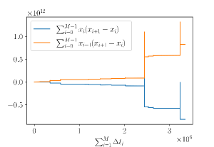
Figure 7. Divergence of $\langle x\dot{x}\rangle$ for Eq. (382).

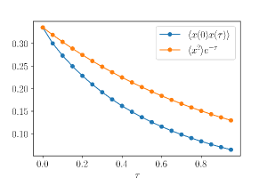
Figure 8. Covariance function for Eq. (382).

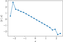
Figure 9. Binned drift function for Eq. (382).

12. Code availability

Code for the simulations is available at https://github.com/yeerenlow/langevin.

13. Acknowledgments

Y.I.L. acknowledges support from the McGill University Department of Physics.

References

- [1] G. J. Stephens, B. Johnson-Kerner, W. Bialek, and W. S. Ryu. Dimensionality and dynamics in the behavior of C. elegans. PLoS Comput. Biol., 4:e1000028, 2008.
- [2] David B. Brückner and Chase P. Broedersz. Learning dynamical models of single and collective cell migration: a review. 2023.
- [3] C. Gardiner. Stochastic Methods. Springer Berlin, Heidelberg, 4 edition, 2009.
- [4] J. B. Weiss. Coordinate invariance in stochastic dynamical systems. Tellus A, 55:208–218, 2003.
- [5] U. Seifert. Stochastic thermodynamics, fluctuation theorems and molecular machines. Rep. Prog. Phys., 75:126001, 2012.
- [6] C. Dieball and A. Godec. Mathematical, thermodynamical, and experimental necessity for corase graining empirical densities and currents in continuous space. Phys. Rev. Lett., 129:140601, 2022.
- [7] C. Battle, C. P. Broedersz, N. Fakhri, V. F. Geyer, J. Howard, C. F. Schmidt, and F. C. MacKintosh. Broken detailed balance at mesoscopic scales in active biological systems. Science, 352:604–607, 2016.
- [8] J. P. Gonzalez, J. C. Neu, and S. W. Teitsworth. Experimental metrics for detection of detailed balance violation. Phys. Rev. E, 99:022143, 2019.
- [9] A. Frishman and P. Ronceray. Learning force fields from stochastic trajectories. Phys. Rev. X, 10:021009, 2020.
- [10] D. B. Brückner, P. Ronceray, and C. P. Broedersz. Inferring the dynamics of underdamped stochastic systems. Phys. Rev. Lett., 125:058103, 2020.
- [11] D. Selmeczi, L. Li, L. I. I. Pedersen, S. F. Nørrelykke, P. H. Hagedorn, S. Mosler, N. B. Larsen, E. C. Cox, and H. Flyvbjerg. Cell motility as random motion: a review. Eur. Phys. J.: Spec. Top., 157:1–15, 2008.
- [12] L. Li, E. C. Cox, and H. Flyvbjerg. “Dicty dynamics”: Dictyostelium motility as persistent random motion. Phys. Biol., 8:046006, 2011.
- [13] F. S. Gnesotto, F. Mura, J. Gladrow, and C. P. Broedersz. Broken detailed balance and non-equilibrium dynamics in living systems: a review. Rep. Prog. Phys., 81:066601, 2018.
- [14] D. Serre (https://mathoverflow.net/users/8799/denis serre). Eigenvalues of sum of a non-symmetric matrix and its transpose . MathOverflow. URL: https://mathoverflow.net/q/52588 (version: 2011-01-20).
- [15] J. Gladrow, N. Fakhri, F. C. MacKintosh, C. F. Schmidt, and C. P. Broedersz. Broken detailed balance of filament dynamics in active networks. Phys. Rev. Lett., 116:248301, 2016.
- [16] I. Mezić. Spectral properties of dynamical systems, model reduction and decompositions. Nonlinear Dyn., 41:309–325, 2005.
- [17] M. O. Williams, I. G. Kevrekidis, and C. W. Rowley. A data-driven approximation of the Koopman operator: extending dynamic mode decomposition. J. Nonlinear Sci., 25:1304–1346, 2015.
- [18] V. R. Kostic, P. Novelli, A. Maurer, C. Ciliberto, L. Rosasco, and M. Pontil. Learning dynamical systems via Koopman operator regression in reproducing kernel Hilbert spaces. Advances in Neural Information Processing Systems, 35:4017–4031, 2022.
- [19] V. R. Kostic, K. Lounici, P. Novelli, and M. Pontil. Sharp spectral rates for Koopman operator learning. In Thirty-seventh Conference on Neural Information Processing Systems, 2023.
- [20] H. Risken. The Fokker–Planck Equation. Springer Berlin, Heidelberg, 2 edition, 1989.
- [21] D. S. Bernstein. Matrix Mathematics. Princeton University Press, 2 edition, 2009.
- [22] G. J. Stephens, M. Bueno de Mesquita, W. S. Ryu, and W. Bialek. Emergence of long timescales and stereotyped behaviors in Caenorhabditis elegans. Proc. Natl. Acad. Sci. U.S.A., 108:7286–7289, 2011.
- [23] F. Ferretti, V. Chardès, T. Mora, A. M. Walczak, and I. Giardina. Building general Langevin models from discrete datasets. Phys. Rev. X, 10:031018, 2020.
- [24] C. Metzner, C. Mark, J. Steinwachs, L. Lautscham, F. Stadler, and B. Fabry. Superstatistical analysis and modelling of heterogeneous random walks. Nat. Commun., 6:7516, 2015.
- [25] D. B. Brückner, A. Fink, J. O. Rädler, and C. P. Broedersz. Disentangling the behavioural variability of confined cell migration. J. R. Soc. Interface, 17:20190689, 2020.