SwarMer: A Decentralized Localization Framework for Flying Light Specks

Abstract.

Swarm-Merging, SwarMer, is a decentralized framework to localize Flying Light Specks (FLSs) to render 2D and 3D shapes. An FLS is a miniature sized drone equipped with one or more light sources to generate different colors and textures with adjustable brightness. It is battery powered, network enabled with storage and processing capability to implement a decentralized algorithm such as SwarMer. An FLS is unable to render a shape by itself. SwarMer uses the inter-FLS relationship effect of its organizational framework to compensate for the simplicity of each individual FLS, enabling a swarm of cooperating FLSs to render complex shapes. SwarMer is resilient to both FLSs failing and FLSs leaving to charge their battery. It is fast, highly accurate, and scales to remain effective when a shape consists of a large number of FLSs.

Source code available at https://github.com/flyinglightspeck/SwarMer. See https://youtu.be/BIiBxD_aUz8 for a MATLAB demonstration of SwarMer, https://youtu.be/Lh11tWWOP5Y for two relative localization techniques as SwarMer plugins. SwarMer is able to transition FLSs from illuminating one point cloud to the next point cloud, see https://youtu.be/4GhhlSq4UrM. It may start with a random pattern and illuminate a shape, see https://youtu.be/cZrz0e61txU. The reported implementation of SwarMer localizes FLSs into a Hat (https://youtu.be/y_xHdz5bs5M), a Dragon (https://youtu.be/PRyjdmw8NVc), and a Skateboard (https://youtu.be/a0fFu0z6BU0).

1. Introduction

An FLS is a miniature sized drone equipped with one or more light sources to generate different colors and textures with adjustable brightness. Synchronized swarms of FLSs will illuminate objects in a pre-specified 3D volume, an FLS display (Ghandeharizadeh, 2021, 2022). The display may be a cuboid that sits on a table (Alimohammadzadeh et al., 2023a) or hangs on a wall, the dashboard of a self-driving vehicle, a room, etc. It will render static 2D or 3D point clouds by assigning the coordinates of their points to different FLSs to illuminate.

An FLS display has diverse multimedia applications ranging from entertainment to healthcare. With entertainment, a photographer may capture 3D point clouds using a depth camera, e.g., Intel RealSense D455, and view them using an FLS display. With healthcare, a physician may illuminate and examine 3D MRI scans of a patient in real time using an FLS display.

Localizing FLSs to render a 2D or a 3D point cloud is non-trivial for several reasons. First, in an indoor setting, FLSs may lack line of sight with GPS satellites to position themselves. Even if GPS was available, it would be too coarse (Saska, 2015; Lee et al., 2016; Ghandeharizadeh, 2021). The best some GPS devices claim is a 3 meter accuracy 95% of the time (Lee et al., 2016; Sun, 2021).

Second, a dead-reckoning technique that requires an FLS to fly to its assigned position is known to suffer from errors that increase as a function of the distance traveled by a drone (Campos et al., 2021; Shurin and Klein, 2022; Chen et al., 2022; Cano et al., 2022). Greater distances result in higher errors, distorting the final rendering. To illustrate, Figure 1.b shows rendering of three 2D point clouds of Figure 1.a (ground truth) using dead reckoning with 5 degrees of error. (See Section 4.1 for a formal definition of the degree of error.) The FLSs are deployed by a dispatcher at the origin, (0, 0). Each FLS uses a collision free path (Guy et al., 2009; Augugliaro et al., 2012; Chen et al., 2015; Hamer et al., 2018; van den Berg et al., 2008, 2011a, 2011b; Stephan et al., 2013; van den Berg et al., 2012; Bareiss and van den Berg, 2013; Arul and Manocha, 2020; Engelhardt et al., 2016; Cheng et al., 2017; Morgan et al., 2013; Báča et al., 2018; Morgan et al., 2014; Tabasso et al., 2021; Cappello et al., 2020; Mylvaganam et al., 2017; Preiss et al., 2017b; Ferrera et al., 2018; Xu et al., 2019; Preiss et al., 2017a; Kushleyev et al., 2013; Jiang et al., 2014) to travel to its coordinate. With dead reckoning, the wing of the butterfly farthest from (closest to) the origin is least (most) accurate because FLSs travel a greater (shorter) distance. With 5 degrees of error, the butterfly wing farthest from the origin is distorted completely, see Figure 1.b. In general, dead reckoning is challenged with realizing symmetrical geometric shapes as simple as a straight line, e.g., the cat’s tail which is close to the dispatcher.

The challenge is to design and implement a general purpose framework that localizes FLSs to render any 2D or 3D shape with an arbitrary amount of dead-reckoning error. This challenge constitutes the focus of this paper. The ideal framework must be:

• Fast. It should localize FLSs as they are deployed. This results in an incremental rendering where portions of a shape become recognizable as other FLSs are deployed to render the remainder of the shape.

• Highly accurate. A rendering should match the intended point cloud. With some applications, this may be an overkill because the human eye may not detect one FLS out of its place even with small point clouds consisting of one hundred FLSs, e.g., compare Figure 1.c with 1.a.

• Continuous. Drones are known to drift (Liu et al., 2017; Gadre et al., 2018). FLSs must be able to execute the algorithm continuously to compensate for both their drift and those of their neighbors.

• Resilient to FLS failures and departures. FLSs are mechanical devices that may fail (Ghandeharizadeh, 2021). Moreover, their battery has a fixed flight time. An FLS must be allowed to fly back to a charging station once its battery is depleted per an algorithm such as STAG (Ghandeharizadeh, 2022). The substituting FLS must be able to localize itself.

• Scalable to render shapes consisting of a large number of FLSs, tens of thousands if not millions.

• Minimal, requiring as few sensors as possible from the display to enhance its flexibility and reduce its cost.

Swarm-Merging, SwarMer, addresses these requirements for 2D and 3D point clouds. It is designed for an in-door 3D display that lacks line of sight with GPS satellites. It is a relative localization system instead of an absolute one, e.g., the teapot of Figure 1.c is moved down relative to its ground truth shown in Figure 1.a. Given a 2D or 3D point cloud, it approximates the position of the FLSs by forcing the neighboring FLSs to match the relative distance and angle (Cano et al., 2022) of their assigned points. Even though the location of each FLS is not exactly the same as that specified by the point cloud, SwarMer’s relative positioning of FLSs produces shapes true to a point cloud. In some instances, there is an exact match between the position of FLSs and the coordinates of points in the point cloud.

SwarMer is a decentralized algorithm, requiring each FLS to localize itself relative to another FLS at a time. Many FLSs may correct their position concurrently and independently. Hence, SwarMer may render a portion of a shape while FLSs are being deployed to complete the rest of the shape. This makes SwarMer fast.

SwarMer constructs swarms (Reynolds, 1987a) of FLSs. Movement of one FLS causes all FLSs in its swarm to move. SwarMer includes provisions that prevent isolated FLSs or fragmented swarms when there should be one swarm. These provisions make SwarMer resilient to FLSs failing and departing to charge their battery.

SwarMer requires FLS to use dead reckoning to position themselves relative to one another repeatedly. Each time, depending on the relative localization technique of the FLSs, the distance traveled by an FLS decreases. Hence, error with inter-FLS dead-reckoning decreases, enhancing SwarMer’s accuracy. See Figure 1.c.

Figures 1.d and 1.e show the use of triangulation and trilateration to localize FLSs. Both are designed for use with anchors that have precise positions (Ledergerber et al., 2015; Zebra, 2018; Corbalán et al., 2019; Chen and Dhekne, 2022; Jung and Weiss, 2022), e.g., GPS satellites (Samama, 2008) used by GPS enabled drones for outdoor light shows. In Figures 1.d and 1.e, an FLS lacks line of sight with a GPS satellite. It uses those FLSs with a high confidence in their location as its anchor with both triangulation and trilateration. The position of these anchors is not 100% precise. This causes triangulation and trilateration to produce distorted shapes.

Assumptions of the SwarMer framework about its FLSs are as follows. First, FLSs are cooperative. Second, an FLS may adjust its radio range by manipulating its transmission power to communicate with FLSs that are farther away (Whitehouse et al., 2007). Third, each FLS has a unique id, FID. FID may be assigned by the FLS hardware, e.g., MAC address of its networking card. Alternatively, a dispatcher (Ghandeharizadeh, 2022) may assign an FID to an FLS as it deploys FLSs. Fourth, an FLS knows its assigned coordinate (a point in a point cloud) and the coordinates of its neighbors. The exact number of neighbors known by an FLS is a tradeoff between the amount of storage required from each FLS and the required network bandwidth for the FLSs to communicate and obtain this information from one another.

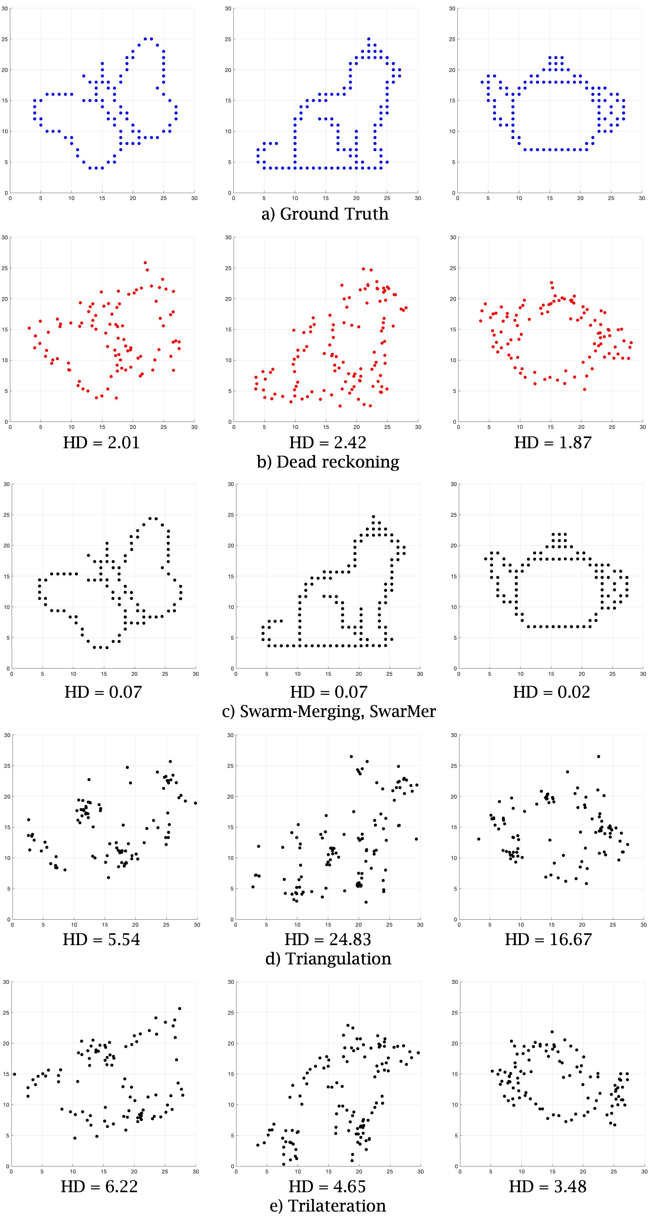
Figure 1. (a) A 2D butterfly, cat, and teapot, (b) illuminations with dead reckoning using $\epsilon$=5 degrees of error, (c) adjustments with swarm-merging using dead reckoning with $\epsilon$=5 degrees of error, (d-e) adjustment with Triangulation and Trilateration using 100% accurate distance and angle.

Contributions of this paper are:

• SwarMer as a relative localization framework to render 2D and 3D shapes. This decentralized framework uses nature inspired swarm concepts. FLSs may execute SwarMer continuously. To the best of our knowledge SwarMer is novel and has not been published elsewhere. (See Section 3.)

• A localization technique is a plugin for the SwarMer framework. We describe two alternative localization techniques using signal strength and physical movement of FLSs relative to one another. In addition, we quantify the tradeoffs associated with these techniques. (See Section 3.1 and https://youtu.be/Lh11tWWOP5Y.)

• Triangulation and trilateration as comparison yardstick to evaluate SwarMer. Obtained results demonstrate the superiority of the SwarMer framework, compare Figure 1.c with 1.d and e. (See Section 5.)

• We present a simulation and an implementation of SwarMer. The MATLAB simulator is used to study and obtain insights into the alternative design decisions. The most promising designs with adjustable configuration parameters are implemented using the Python 3.9 programming language with UDP sockets. We are actively exploring their deployment in a swarm of drones. (See Section 6.)

• We open source our software implementations, and the 2D and 3D data used in this study for further use and investigation by the scientific community. See https://github.com/flyinglightspeck/SwarMer for details.

• A limitation of SwarMer is that it may shift a shape along different dimensions. It requires an accurate reference point or an oracle FLS to address this limitation. (See Section 4.2.4.)

The rest of this paper is organized as follows. Section 2 provides the terminology used by this paper and a formal statement of the localization problem. Section 3 presents SwarMer. We evaluate SwarMer using 2D and 3D point clouds in Section 4. Section 5 provides our Matlab implementation of triangulation and trilateration, comparing them with SwarMer. Section 6 presents an emulation of SwarMer. Related work are described in Section 7. Section 8 presents our future research directions.

2. Terminology, Problem Statement

Given the novelty of FLSs and a 3D FLS display, this section introduces terminology for concepts in order to state the problem solved by SwarMer. We use this terminology throughout the paper. The SwarMer framework is independent of the assumed terminology and may use alternative ontologies that match the concepts per definitions provided in this section.

To render an illumination, an FLS display constructs a 3D mesh on the display volume. A cell of this mesh, a display cell (Ghandeharizadeh, 2022), is dictated by the downwash of an FLS (Arul and Manocha, 2020; Preiss et al., 2017b; Bareiss and van den Berg, 2013; Ferrera et al., 2018; Xu et al., 2019). Assuming an FLS is a quadrotar, a cell may be an ellipsoid (Arul and Manocha, 2020; Preiss et al., 2017b; Bareiss and van den Berg, 2013) or a cylinders (Ferrera et al., 2018; Xu et al., 2019) that results in a larger separation along the height dimension. Each display cell has a unique Length, Height, and Depth (L,H,D) coordinate (Ghandeharizadeh, 2022). We use the L, H, D coordinate system instead of X, Y, Z to identify a cell because there is no consensus on one definition of the Y and Z axes. While the picture industry uses the Z axis as the depth, mathematicians use the Y axis for the depth. It is trivial to map our L, H, D coordinate system to either definition without ambiguity.

We assume a fixed coordinate system for the FLS display with (0, 0, 0) as its bottom left corner. Moreover, we assume the geometry of a 3D point cloud identifies the location of a display cell in an illumination cell. This is the (L,H,D) coordinate of a point assigned to an FLS to illuminate.

Definition 2.0.

Ground truth is the ideal location and orientation of an FLS in an FLS display. It is dictated by the geometry of a point cloud, the (L,H,D) coordinates of a point. An FLS is assigned the coordinates of a point in the ground truth to illuminate.

Definition 2.0.

Estimated truth is the actual location and orientation of an FLS in an FLS display. It is an FLS’s estimate of the ground truth and may match the ground truth with some degree of accuracy including perfect (100%) accuracy.

Definition 2.0.

A vector $\vec{i,j}$ exists between any two points $i$ and $j$ in a point cloud. It has a fixed length $|\vec{i,j}|$. With 2D point clouds, it has an angle $\alpha$ relative to the horizontal L-axis. With 3D point clouds, in addition to $\alpha$, it has an angle $\theta$ relative to the height, H-axis, of a display. See Figure 4.

Problem Definition 1.

Given a 2D (3D) point cloud with each point assigned to a unique FLS, localize FLSs to minimize the Hausdorff distance (Huttenlocher et al., 1993) between the estimated truth and the ground truth.

Section 2.1 provides a formal definition of how we compute the Hausdorff distance (Huttenlocher et al., 1993). Hausdorff distance is used to quantify SwarMer’s accuracy and SwarMer is independent of it.

2.1. Hausdorff Distance, HD

We use the Hausdorff distance (Huttenlocher et al., 1993) to compare the FLS rendering E, i.e., the estimated truth, with the ground truth G, Hausdorff(E,G) or HD for short. This metric reports the maximum error in distance between E and G after applying a translation. A lower value is better with zero reflecting a perfect match between E and G. Below we describe how we compute the maximum error and our translation process in turn.

To compute the maximum error between E and G, for each coordinate $e_{i}$ in E, we find the minimum distance between $e_{i}$ and the coordinate $g_{j}$ of each point $j$ in G. Let {EG} denote this set of values. Next, for the coordinate of each point $g_{i}$ in G, we compute the minimum distance between $g_{i}$ and the coordinate of each FLS $e_{j}$ in E. Let {GE} denote this set of values. The Hausdorff distance is the maximum of the values in these two sets, HD = max(max({EG}), max({GE})).

The translation of E to G with the MATLAB simulator of Section 4 is different than with the implementation of Section 6. With the simulator, we translate E to G using the following stochastic technique. We select $\{R\}$ random FLSs from E; $|R|$=90 FLSs in all our experiments. For each FLS $i$ in $\{R\}$, we identify its assigned point in G. We compute the vector $\vec{D_{i}}$ that reduces the distance between the pair to zero. We apply $\vec{D_{i}}$ to the $\{R\}$ FLSs and compute the sum of errors between the $\{R\}$ FLSs and their assigned points in G, $E_{i}=\sum_{j=1}^{|R|}e_{j}-g_{j}$. We identify the FLS $k$ with minimum error $E_{k}$ ($1\leq k\leq|R|$). Our translation process applies vector $\vec{D_{k}}$ to all FLSs in E. Subsequently, we compute HD. The complexity of this stochastic technique is $90\times(90+3\times 90)+F$ since it applies each translation to 90 points, computes the distance between each pair of 90 corresponding points, and sums them. Then applies the one with the minimum sum of distances to the $F$ FLSs. More generally, the complexity is O($c\times|R|^{2}+F$) where c is a constant.

With the implementation, we compute the center of each point cloud $E$ and $G$, $C_{E}$ and $C_{G}$, respectively. We compute a vector $\vec{D}=C_{G}-C_{E}$ We add all $\vec{D}$ to each point in the point cloud E. Finally, we compute HD. The complexity of computing the center of each point cloud is O($F$) where F is number of FLSs. With the additional scan of E to apply $\vec{D}$, the overall complexity is O($3F$).

The translation process is required because SwarMer is a relative localization technique.

3. Swarm-Merging (SwarMer)

SwarMer is a decentralized algorithm that assumes the error in dead reckoning decreases when FLSs travel shorter distances. A dispatched FLS travels to its assigned destination using dead reckoning. When it arrives at its destination, SwarMer requires the FLS to localize relative to its neighbors using dead reckoning repeatedly. This reduces the travelled distance to enhance the accuracy of dead reckoning, enabling the FLS to approximate the ground truth more accurately.

As soon as an FLS $F_{i}$ arrives at its destination, it constructs a swarm consisting of itself with its Swarm-ID set to its FID, $\xi_{i}$=$i$. Next, $F_{i}$ expands its radio range to identify an FLS $F_{j}$ with a different swarm-id, $\xi_{i}\neq\xi_{j}$. $F_{i}$ challenges $F_{j}$ to merge into one swarm. Assuming $F_{j}$ accepts the challenge, the one with a lower Swarm-ID becomes the anchor FLS and the other becomes the localizing FLS. Assuming $\xi_{i}<\xi_{j}$, the localizing FLS, $F_{j}$, computes a vector $\vec{V}$ for its movement relative to its anchor $F_{i}$ to better approximate the ground truth. Section 3.1 describes two techniques to compute $\vec{V}$.

An FLS maintains a binary status property initialized to available. Its other possible value is busy. When $F_{j}$ is challenged and its status is available then it changes its status to busy and notifies the FLSs that constitute its swarm to change their status to busy. $F_{i}$ also changes its status to busy and informs those FLSs in its swarm to change their status to busy. Each message includes whether the swarm is localizing or anchor. $F_{i}$ and $F_{j}$ determine this independently, by comparing their Swarm-ID, $\xi_{i}$ and $\xi_{j}$. With $\xi_{i}<\xi_{j}$, in addition to the busy status change, $F_{i}$’s ($F_{j}$’s) message includes the anchor (localizing) flag.

An available FLS accepts a challenge always. A busy FLS accepts a challenge only if it is an anchor and its Swarm-ID is lower than that of a challenger. This FLS will serve as the anchor for the challenger. An FLS may serve as the anchor for multiple localizing FLSs beloning to different swarms. Moreover, different FLSs belonging to the same swarm may serve as anchors for multiple localizing FLSs belonging to different swarms. Hence, SwarMer may merge two or more swarms ($M\geq 2$) into one.

Once $F_{j}$ computes a vector $\vec{V}$ for its movement relative to $F_{i}$, $F_{j}$ informs members of its swarm to change their Swarm-ID to $F_{i}$’s Swarm-ID ($\xi_{i}$) and move along $\vec{V}$. $F_{j}$ changes its Swarm-ID to $F_{i}$’s Swarm-ID ($\xi_{i}$) and moves along $\vec{V}$ to localize itself relative to $F_{i}$. Next, it changes its status from busy to available. $F_{j}$’s local movement and status change may occur concurrently with its message transmission to the members of its swarm. Members of $F_{j}$’s swarm change their Swarm-ID to $\xi_{i}$, move along $\vec{V}$, and change their status to available independently. Finally, $F_{j}$ notifies $F_{i}$ to unanchor itself, enabling it to localize relative to other FLSs. This completes merging of the $F_{i}$ and $F_{j}$ swarms into one with the participating FLS’s Swarm-ID set to $\xi_{i}$.

SwarMer localizes FLSs using their nearest neighbor by requiring an FLS to expand its radio range. FLSs must measure distance and angle relative to one another to localize.

Definition 3.0.

A swarm consists of a collection of FLSs with the same Swarm-ID $\xi$. $\xi$ is set to the minimum FID of the FLSs in the swarm. FLSs that constitute a swarm move together (Reynolds, 1987b; Wang et al., 2015a).

Definition 3.0.

A localizing FLS has a Swarm-ID greater than its anchor FLS. It informs all members of its swarm to change their status to busy, preventing them from localizing relative to a different swarm. It computes a new coordinate and orientation $\phi$ relative to its anchor FLS. Both are in the FLS’s estimated truth. Using its current and new coordinates, it computes a vector $\vec{V}$ to travel to its new coordinate. The FLS informs all members of its swarm to change their Swarm-ID to that of its anchor FLS, move along $\vec{V}$ using dead reckoning, and orient themselves using $\phi$. The FLS changes its Swarm-ID to that of the localizing FLS, uses dead reckoning to travel along vector $\vec{V}$ to its new coordinate, and orients itself using angle $\phi$. The localizing FLS and members of its swarm move along $\vec{V}$ as long as $\vec{V}$’s magnitude exceeds a threshold. The localizing FLS changes its status to available and notifies the anchor FLSs to change its status to available.

Definition 3.0.

An anchor FLS remains stationary and changes its status to busy, enabling one or more localizing FLSs belonging to different swarms to compute a vector $\vec{V}$ and orientation $\phi$ relative to it. It has a Swarm-ID lower than its localizing FLSs. It notifies members of its swarm to change their status to busy, preventing them from localizing.

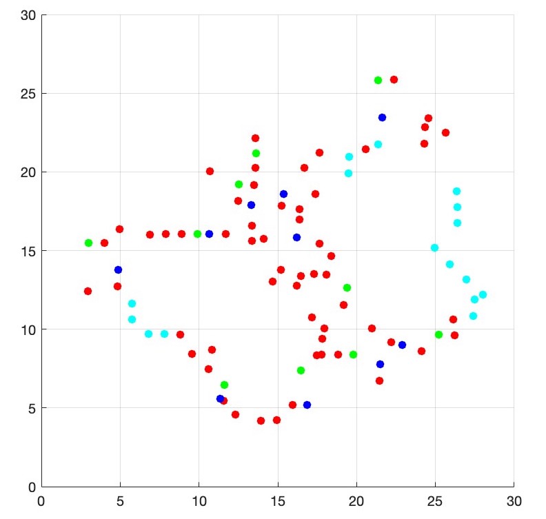
Figure 2. Greens and dark blues are localizing and anchored FLSs, respectively. Members of their swarms are in red. Available FLSs are in light blue.

FLSs belonging to different swarms may localize concurrently. One or more FLSs of a swarm may serve as the anchor for different localizing FLSs. Figure 2 shows 10 localizing FLSs (green), their anchored FLSs (dark blue), members of their swarms (red), and available FLSs (light blue).

When an FLS expands its radio range, it may encounter $M-1$ FLSs with different Swarm-IDs. The FLS with the lowest Swarm-ID becomes the anchor while $M-1$ FLSs localize relative to it. This merges $M$ swarms into one. SwarMer may limit the value of M to 2 or higher ($\infty$), e.g., 2 for binary merging of swarms. The value $\infty$ merges as many candidates as possible.

SwarMer may use different techniques to select the identity of the anchor swarm. Thus far, we have described the Lowest Swarm-ID, a simple technique that uses the FLS with the lowest Swarm-ID as the anchor. A more complex technique is to use the FLS belonging to the swarm with the most number of FLSs as the anchor FLS. It may require an FLS to use a decentralized peer-to-peer technique to estimate the size of its swarm (Bawa et al., 2003). In case of ties with multiple swarms having the same size, the one with the lowest Swarm-ID may serve as the anchor. Section 4.2.2 evaluates four techniques. It shows while one technique may be superior for a specific point cloud, no technique is superior across all point clouds. Hence, we use the lowest Swarm-ID for the rest of this section.

With $F$ FLSs, the number of rounds performed by SwarMer to construct one swarm is $log~{}F$. With $M$=2, the number of rounds is deterministic. With $M$=$\infty$, the base of the log is a function of the average number of swarms merged in a round. It depends on the density of the point cloud and how many swarms are merged at a time. See discussions of Figure 19.

Multiple FLSs, say $\mu$, of a swarm may race with one another to localize relative to different FLSs belonging to different anchor swarms concurrently. This results in a race condition between $\mu$ localizing FLSs generating different vectors for the FLSs of the localizing swarm. SwarMer ensures FLSs of the localizing swarm applies at most one vector, discarding $\mu-1$ vectors. This partitions the localizing swarm into $\mu$ swarms. A localizing FLS that uses anchor FLS $F_{i}$ generates a message containing its Old Swarm-ID ($\xi_{O}$), New Swarm-ID ($\xi_{Ni}$), and its computed vector. There are $\mu-1$ messages with different $\xi_{Ni}<\xi_{O}$ racing with one another. A receiving FLS compares its Swarm-ID with $\xi_{O}$ contained in the message. If they are equal then it sets its Swarm-ID to $\xi_{Ni}$ and travels along the provided vector in the message. This FLS will discard the $\mu-1$ messages since its Swarm-ID $\xi_{Ni}$ does not equal to the old Swarm-ID of the messages. The consequence is that the localizing swarm is fragmented into $\mu$ swarms. These swarms will subsequently localize relative to one another and merge into one.

To illustrate, assume FLSs A and B of Swarm 3 localize relative to an FLS of two different swarms with Swarm-IDs 1 and 2. FLSs A and B issue a Busy message to all FLSs that constitute Swarm 3. After localizing, FLSs A and B generate a message with their independently computed vector, $\xi_{O}$=3, and the new Swarm-ID $\xi_{N}$={1 or 2}. These messages race with one another. A receiving busy FLS $F_{k}$ with Swarm-ID $\xi_{k}$=3 changes its Swarm-ID to the Swarm Id of the winner message (say 1, $\xi_{k}$=1). $F_{k}$’s swarm-ID $\xi_{k}$=1 does not match the loser’s message with $\xi_{O}$=3, causing $F_{k}$ to discard this message. Thus, one vector is applied by a unique and distinct subset of FLSs that constitute Swarm 3, fragmenting Swarm 3 into two swarms with two different Swarm IDs, 1 and 2.

As swarms merge and form larger swarms, SwarMer saves battery power of FLSs by requiring only those FLSs with a missing neighbor to expand their radio range. This saves battery power of many FLSs by preventing them from expanding their radio range only to discover FLSs that decline their challenge to merge. FLSs with no missing neighbors are termed Relatively-Complete, R-Complete. They wait to be challenged.

Definition 3.0.

An FLS is Relatively Complete, R-Complete, once its expands its radio range and discovers $\eta$ FLSs in its estimated truth that match its ground truth and have its Swarm-ID, i.e., they are a part of the same swarm. An R-Complete FLS does not expand its radio range and does not challenge other FLSs to join its swarm. The value of $\eta$ is adjustable and maybe customized for efficient rendering of a point cloud.

SwarMer imposes the following requirement on all FLSs. A swarm consisting of an FLS with busy neighbors belonging to a different swarm is required to localize itself relative to one of the neighbors and join its swarm. This requirement makes SwarMer resilient to FLS failures and FLSs leaving to charge their battery. In both cases, a new FLS arrives to substitute for the departing FLS. The requirement causes this new FLS to localize and join the existing swarm immediately. In addition, this requirement prevents formation of multiple disjoint swarms that should be one with small values of $\eta$.

One may configure SwarMer to localize FLSs continuously. Once all FLSs constitute one swarm, they may thaw their swarm membership. Each FLS resets its Swarm-ID to its FID, Swarm-ID=FID. This forms swarms consisting of one FLS without impacting the position of each FLS. Next, the FLSs repeat the localization process of SwarMer. Section 4.2 shows repeated application of SwarMer enhances the quality of a rendering, i.e., lowers the Hausdorff distance. This repetition is fast. Section 6 shows SwarMer drops the Hausdorff distance to a value below 0.01 after a few repetitions in tens of seconds.

There are multiple ways of thawing the final swarm in a decentralized manner. One approach may require an FLSs to periodically estimate the size of its swarm using a decentralized counting technique such as (Bawa et al., 2003). Each FLS may be provided with the size of the point cloud when it is deployed. Once the two numbers are approximately the same then the FLS broadcasts a thaw message. All FLSs that receive the thaw message reset their SwarmID to their respective FID and repeat the thaw message with some probability.

An alternative approach may require those FLSs at the farthest corner of an illumination to set a timer once they are R-Complete. When this timer expires, an FLS expands its radio range to the maximum possible and generates a thaw message, announcing its Swarm-ID. If a receiving FLS has a different Swarm-ID then it broadcasts a message to abort swarm thawing, causing the transmitter to sleep and try again. Otherwise, it repeats the thaw message using its Swarm-ID with some probability. Once an FLS receives a fixed number of thaw messages, it sets its Swarm-ID to its FID and repeats the localization process using SwarMer. An evaluation of these alternatives is a future research direction.

3.1. Relative Localization

This section describes two techniques for a localizing FLS to position itself relative to an anchor FLS. They are plugins for the SwarMer framework and may be implemented using a variety of techniques described in Section 3.1.1.

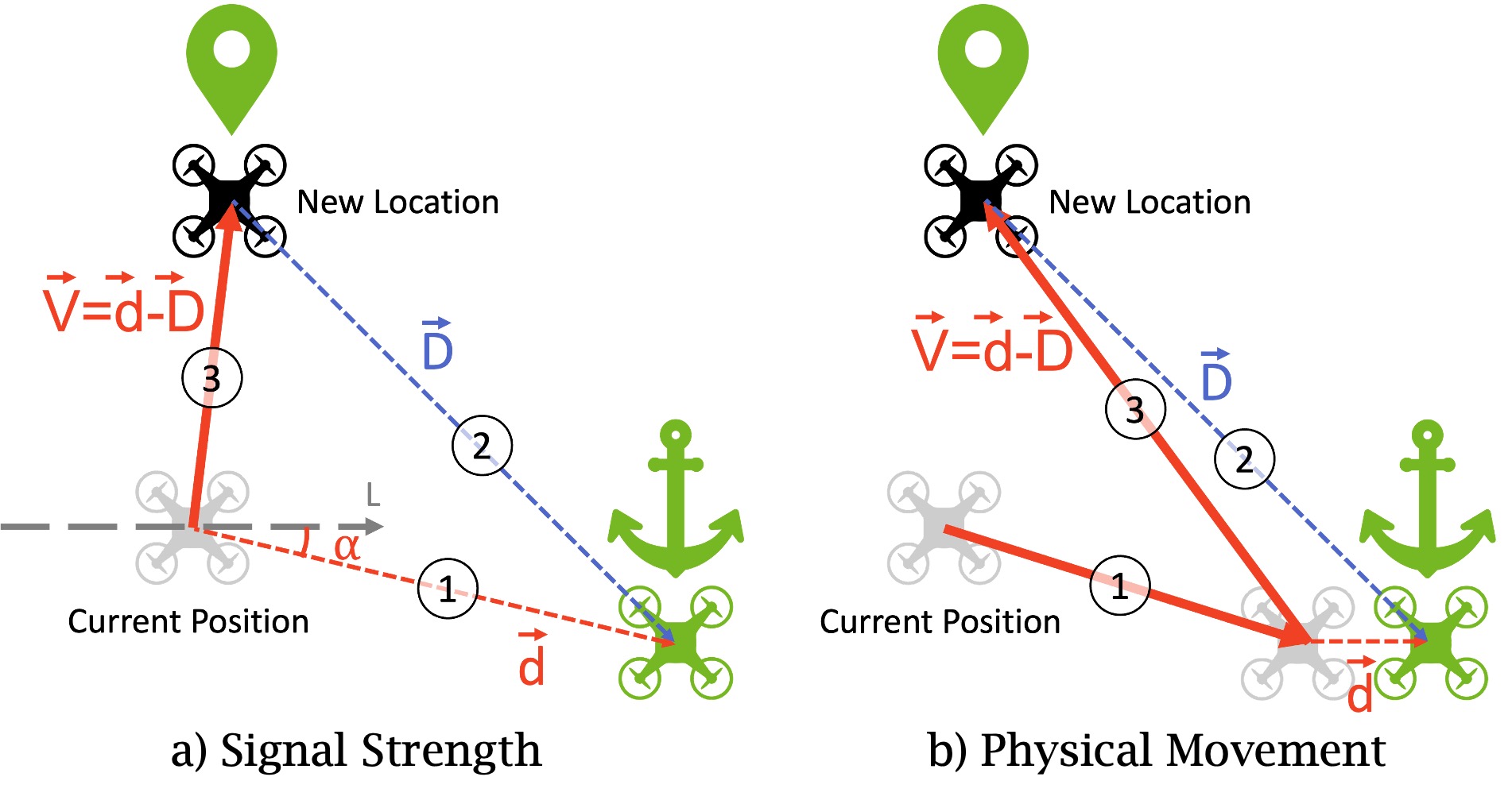
Figure 3. SwarMer FLS Localization in 2D.

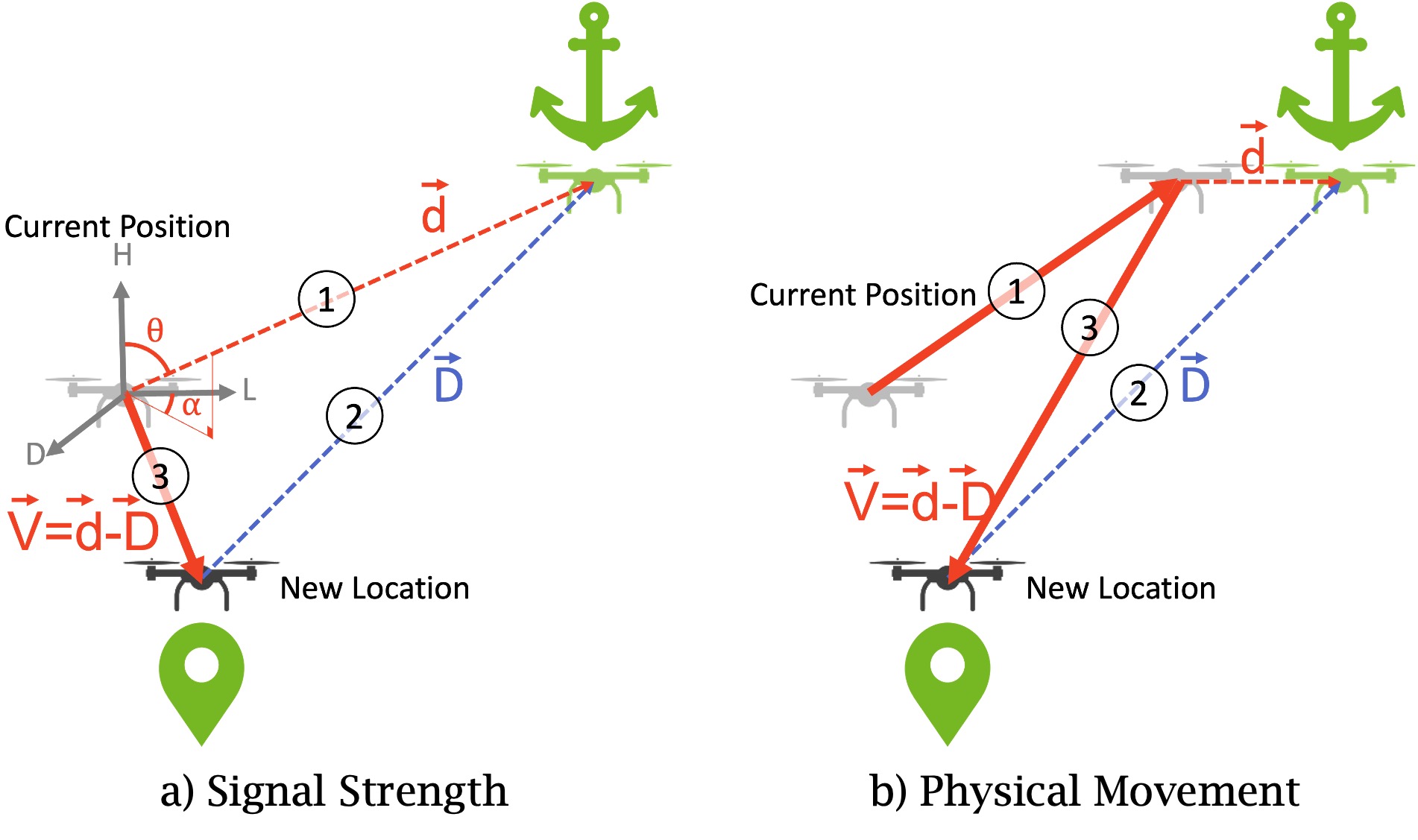
Figure 4. SwarMer FLS Localization in 3D.

The first technique, Signal Strength (SS), assumes an FLS (a) has sensors to detect both the angle and the strength of the signal received from another FLS, and (b) may convert these sensor readings to distance from the FLS generating the signal. One may consider and evaluate alternative sensors when designing and implementing SS with FLSs. Bluetooth (Wang et al., 2015b; Obreja and Vulpe, 2020), Wi-Fi (Rubina et al., 2017; Retscher, 2020), RFID (Wu et al., 2020; Zhang et al., 2019; Patel and Zawodniok, 2022; Bernardini et al., 2021), UWB (Macoir et al., 2019; Silva et al., 2014; Lazzari et al., 2017), Lidar (Cho et al., 2022; Song et al., 2016), RGB cameras (Zhang et al., 2020; Beinschob et al., 2017; Pavliv et al., 2021; Song et al., 2016) and infrared (Kushleyev et al., 2013; Ritz et al., 2012; Preiss et al., 2017b) may be used to obtain distance information. The angle information may be obtained by mounting an antenna array on an FLS, e.g., Bluetooth (Wang et al., 2021b), Wi-Fi (Tong et al., 2021). Angle of Arrival, AOA (Xiong and Jamieson, 2013), obtains the angles at which the signal sent by a localizing FLS reaches the antennas mounted on an anchor FLS. Several surveys document the alternative sensor technologies, their strengths and weaknesses (Chen et al., 2022; Gu et al., 2009; Mainetti et al., 2014; Zafari et al., 2019).

In 2D, SS requires the localizing FLS to request the anchor FLS to generate a signal. It uses its sensors to estimate vector $\vec{d}$. This vector is defined using angle $\alpha$ relative to the L-axis with distance —d— from the anchor FLS, see Step 1 in Figure 3.a. Next, the localizing FLS uses the ground truth to calculate vector $\vec{D}$. The tail (head) of $\vec{D}$ is the position of the localizing (anchor) FLS in the ground truth, see Step 2 in Figure 3.a. We subtract the two vectors to obtain $\vec{V}$, $\vec{V}=\vec{d}-\vec{D}$. The localizing FLS moves along vector $\vec{V}$ to its new position, see Step 3 in Figure 3.a.

The second technique, named Physical Movement (PM), requires the localizing FLS to position itself next to the anchor FLS using its Inertial-Measurement-Unit, IMU. Step 1 of Figure 3.b shows this step in 2D. Next, the localizing FLS computes its angle and distance from the anchor FLS in the ground truth, vector $\vec{D}$ of Step 2 in Figure 3.b. It also computes its displacement vector relative to the anchor, Vector $\vec{d}$. We subtract the two vectors to obtain $\vec{V}$, $\vec{V}=\vec{d}-\vec{D}$. The localizing FLS moves along vector $\vec{V}$ to its new position, see Step 3 in Figure 3.b.

In 3D, SS must also compute the angle $\theta$ relative to the height H, see Figure 4.a. PM uses a similar angle implicitly (not shown in Figure 4.b) as a part of its Step 1.

Figure 5. A comparison of SS with PM, $\epsilon$=5$\degree$.

Figure 6. Dead reckoning distance for the 2D Butterfly of Figure 5.

Figure 7. Hausdorff distance for the 2D Butterfly of Figure 5.

Generally, the dead reckoning distance travelled by a localizing FLS is greater with PM when compared with SS. This results in a higher error with PM, enabling SS to provide more accurate renderings. To illustrate, Figure 6 shows the dead reckoning distance with the 2D butterfly. Generally, SS reduces this distance somewhere between a factor of 5x to 10x with 2D shapes. This increases the accuracy of the rendered shapes, see Figure 5.a. Figure 7 shows the Hausdorff distance for the two alternatives with the 2D butterfly. The Hausdorff distance decreases close to zero with SS because the dead reckoning distance is decreasing as a function of the number of iterations, see Figure 6. PM does not realize the same.

The x-axis of Figures 6 and 7 is an estimate of time. SS approximates the ground truth faster than PM.

With SS, the average dead reckoning distance and Hausdorff distance do not decrease monotonically as a function of the rounds. Figures 9 and 10 show this for the 2D butterfly of Figure 8 consisting of 1008 FLSs. This shape requires FLSs to be aligned in straight lines. SS is more effective than PM in realizing these lines, compare Figure 8.a with 8.b.

Figure 8. A comparison of SS with PM, $\epsilon$=5$\degree$.

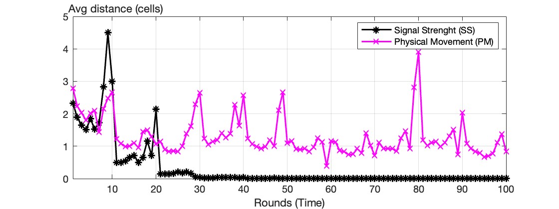
Figure 9. Dead reckoning distance for the 2D Butterfly of Figure 8.

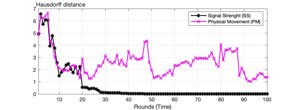
Figure 10. Hausdorff distance for the 2D Butterfly of Figure 8.

In summary, SS is both faster and more accurate than PM. It is also more energy efficient by minimizing the distance traveled by FLSs. This maximizes the flight time of an FLS on a fully charged battery. These observations hold true with both 2D and 3D shapes.

3.1.1. Possible Implementations of SS

Relative state estimation techniques have been an active area of research and they may be the basis of an SS implementation. Some studies use radio technology such as Ultra-WideBand (UWB) to measure distance to estimate the relative 3-DOF location between UAVs (Ledergerber et al., 2015; Alarifi et al., 2016; Großiwindhager et al., 2019). They report measuring distances exceeding 5-7 cm accurately (Großiwindhager et al., 2019; Ledergerber et al., 2015). Some techniques use the odometry information to refine UWB measurements (Zhiqiang et al., 2021).

Visual odometry techniques (Klein and Murray, 2007; Engel et al., 2018; Klose et al., 2010; Babinec et al., 2014) will equip each FLS with an onboard camera to observe other FLSs in its field of view (FoV). They require a texture rich and a well-lit environment. Their accuracy is dictated by the FoV of the on-board camera (Xu et al., 2020, 2022).

Several studies synergize the strength of different sensors by fusing their measurements to enhance accuracy. There are techniques to integrate WiFi access points with IMU (Xie et al., 2018; Xiao et al., 2023), IMU with visual features from a camera (Mur-Artal and Tardós, 2017; Qin et al., 2018; Geneva et al., 2020), LiDAR with odometry (Dube et al., 2017; Zhang and Singh, 2014; Wang et al., 2021a; Lin and Zhang, 2020), UWB with IMU and images from a camera (Xu et al., 2020, 2022; Kao et al., 2023; Yang et al., 2021), UWB with IMU and LiDAR (Nguyen et al., 2021). Laser-based approaches such as LiDaR are highly accurate. However, they may not be suitable for use with FLSs due to their required power, weight, and cost (Xiao et al., 2023).

To evaluate a candidate technology, one must evaluate their scalability to thousands and millions of FLSs to illuminate 2D and 3D shapes.

3.2. FLS Failure and Battery Charging

An FLS is a mechanical device that may fail. One may use the concept of leases (Gray and Cheriton, 1989; Ghandeharizadeh et al., 2014) to prevent failure of a localizing FLS from causing another FLS to remain anchored indefinitely. When a localizing FLS requests another FLS to serve as its anchor, the anchored FLS grants a lease with a fixed duration $\delta$ to the localizing FLS. The localizing FLS must renew this lease prior to its expiration, i.e., $\delta$ time units. Otherwise, the anchored FLS will assume the localizing FLS has failed and will un-anchor itself, i.e., change its status to available.

When an anchor FLS fails, as long as the localizing FLS has sufficient information to localize then it localizes, informs the members of its swarm to update their Swarm-ID to that of the failed anchor FLS, and changes its status to available. SwarMer uses leases to detect failures in an asymmetric manner: Failure of the anchor does not impact the localizing FLS and leases do not detect a failed anchor FLS. SwarMer uses leases to detect failure of the localizing FLS, causing the anchor FLS to unanchor itself.

A standby FLS (Ghandeharizadeh, 2022) will substitute for a failed FLS as follows. It uses dead reckoning to move to the location of the failed FLS and localizes itself relative to a neighbor.

When the battery flight time of an FLS is below a threshold (see STAG (Ghandeharizadeh, 2022)), it notifies its neighbors and the standby that it is leaving the swarm. While it flies back to a charging station, a standby FLS assumes its lighting responsibility per the aforementioned discussion of failure handling.

4. An Evaluation

This section evaluates SwarMer using several 2D and 3D point clouds, see Figures 1.a and 12.a. This evaluation uses a simulation model of SwarMer implemented in MATLAB. Given a point cloud, it assigns a point to an FLS and implements dead reckoning to compute the location of the FLS deployed from a dispatcher at a well known coordinate. This dead reckoning technique is described in Section 4.1. SwarMer uses this technique repeatedly to localize FLSs.

The simulator executes in rounds. At the start of each round, an FLS executes the algorithm of Section 3. We quantify (a) the minimum, average, and maximum number of FLSs that SwarMer localizes in each round, (b) the minimum, average, and maximum distance traveled by FLSs during each round, (c) the number of swarms at the end of each round, (d) the HD at the end of each round.

This evaluation uses standard PNG images for 2D point clouds and the Princeton Shape Benchmark (Shilane et al., 2004) for 3D point clouds. With PNG images, we wrote software to convert it into 2D point clouds, see Figure 1.a. The Princeton benchmark consists of a database of 1,814 3D models. We wrote software to convert its shapes to 3D point clouds. A few are shown in Figure 12.a.

4.1. Dead reckoning

An FLS has a starting position $S$ and a destination $D$ in the ground truth, see Figure 11. Vector $\vec{SD}$ at angle $\theta$ has a fixed length $L$. The error in dead reckoning is bounded by the angle $\epsilon$, $\theta\pm\epsilon$. In 2D (3D), see Figure 11.a (11.b), there is a radius $R_{max}$ for the circular-arc (spherical dome) defined by $\epsilon$. $R_{max}$ increases as a function of $\epsilon$ and $L$.

(a) 2D.

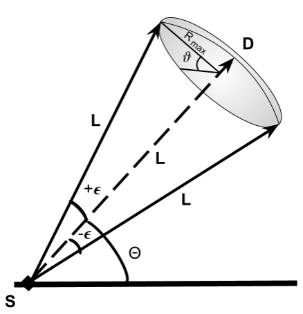
(b) 3D.

Figure 11. Angle of error $\epsilon$ with dead reckoning.

In 3D, in addition to $\epsilon$, another random number $\vartheta$ between 0 and $2\pi$ radian (i.e., 0 and 360 degrees) is used to decide the direction in which the epsilon should be added to the vector. Figure 11.b shows $\vartheta$ in the spherical dome.

The value of $\epsilon$ is a configuration parameter of the simulator and defines $R_{max}$ in Figure 11. Every time an FLS invokes dead reckoning, the simulator generates a random value between $\pm\epsilon$. It adds this angle to $\theta$ to compute a vector with length $L$ starting at S. The point $D$ at the end of this vector is the destination of an FLS and its coordinate in the estimated truth. The FLS flies to this coordinate.

4.2. Experimental Results

Figure 1 shows SwarMer localizes FLSs to approximate the ground truth with $\epsilon$=5$\degree$, compare Figure 1.c with Figure 1.a. These 2D point clouds consist of approximately 100 FLSs. SwarMer employs dead reckoning with the Signal Strength technique (see Section 3.1) and $\eta$=5. It reduces error by minimizing the distance traveled by localizing FLSs.

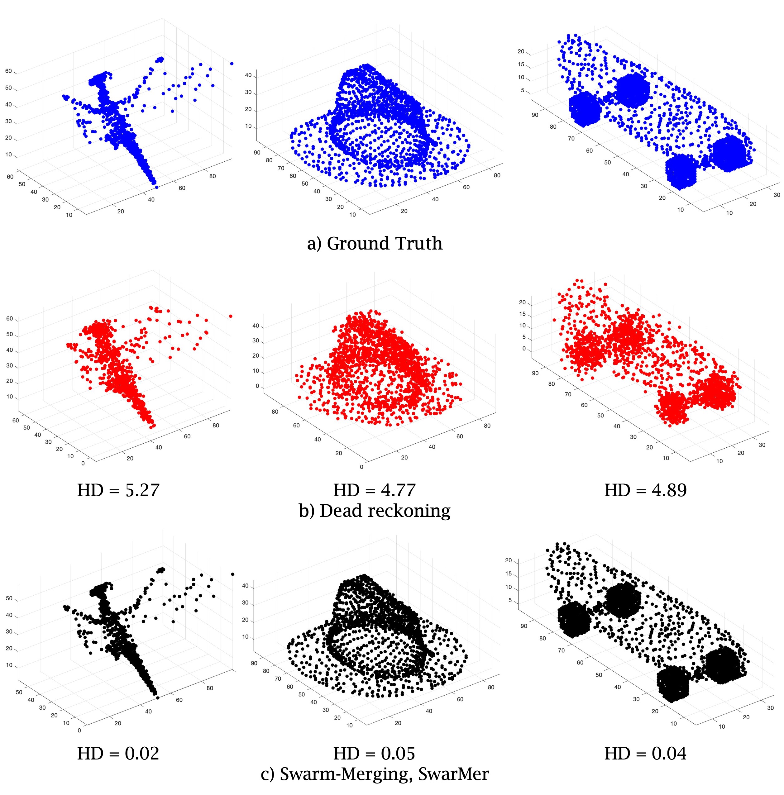
Figure 12. (a) Ground truth for a 3D dragon, a hat, and a skateboard, (b) illuminations with dead reckoning using $\epsilon$=5$\degree$ and a random $\vartheta$ between 0 and 360 degrees, (c) adjustments with n-ary SwarMer using dead reckoning with $\epsilon$=5$\degree$ and a random $\vartheta$ between 0 and 360 degrees.

Figure 12 shows several 3D point clouds from the Princeton Benchmark that challenged our earlier attempts at developing a localizing algorithm. The dragon, hat, and skateboard consist of 760, 1562 and 1727 points (FLSs), respectively. Figure 12.b shows dead reckoning by itself results in renderings that are distorted. These are enhanced by SwarMer, resulting in a low HD, see Figure 12.c. In these experiments, SwarMer merges multiple swarms together at a time, n-ary merging technique of Section 3. Section 4.2.1 compares this with binary that merges two swarms at a time.

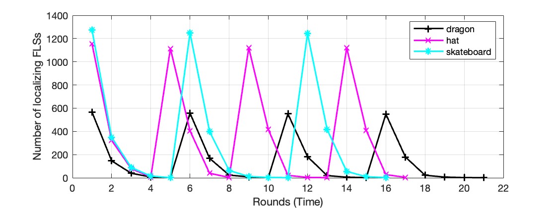
Figure 13. Localizing FLSs for different 3D shapes, $\epsilon$=5$\degree$.

Figure 13 shows the number of localizing FLSs for the different 3D shapes as a function of the number of rounds. The number is lowest with the dragon because it consists of the fewest number of points. As the FLSs form swarms, the number of localizing FLSs decreases. Once there are no localizing FLSs, there is one swarm consisting of all FLSs. Different 3D shapes arrive at this point at different rounds: Round 4 with the hat, and Round 5 with both the dragon and the skateboard. SwarMer is a continuous framework. Once all FLSs constitute a single swarm, all FLSs thaw their swarm memberships and localize again. In our simulation studies, we artificially terminated the simulation once there is a single swarm with a HD lower than 0.09. SwarMer reaches this threshold at a different round for different point clouds. While it forms and thaws a single swarm twice with the skateboard, the count is thrice with the hat and the dragon; count the peaks in Figure 13.

Figure 14. HD.

Below, we focus on the results obtained from the dragon. Figure 14 shows SwarMer’s HD with different degrees of error, i.e., $\epsilon$ values of 1, 3, and 5 degrees, as a function of the number of rounds. A lower HD is better because it shows the rendering approximates the ground truth more accurately. This distance decreases as a function of the number of rounds. With $\epsilon$=1$\degree$, the simulation terminates in the 5th round because its HD drops below 0.09.

Figure 15. Number of swarms.

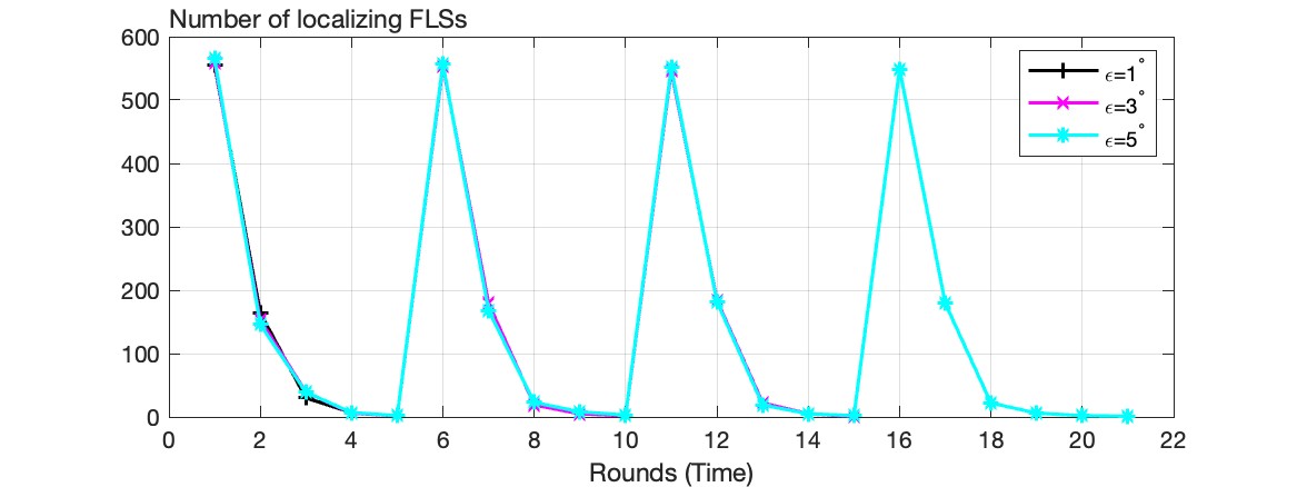
Figure 16. Number of localizing FLSs.

Figure 17. Number of anchor FLSs.

SwarMer forms swarms starting in the first round, see Figure 15. The number of localizing FLSs in each round is approximately the same for different $\epsilon$ values, see Figure 16. It is more than 2x the number of anchor FLSs, see Figure 17 and compare with Figure 16. This is because multiple swarms are merged in each round, see Figure 19.

Figure 18. Average dead reckoning distance.

Figure 18 shows the average dead reckoning distance as a function of the number of rounds. This distance is greater with a higher dead reckoning error. Generally speaking, this distance decreases as a function of the number of rounds but not always, see $\epsilon$=5$\degree$ in Figure 18.

4.2.1. Number of Merged Swarms

An anchor FLS may have multiple localizing FLSs as its candidates. It may proceed with at least one localizing FLS or multiple of them. The former merges two swarms (swarm of the localizing FLS and the anchor FLS) together while the latter may merge a large number of swarms, $\infty$ in theory. This configuration parameter of SwarMer is denoted as M. The results presented in the previous section are with M=$\infty$.

When considering the extreme values of M, 2 and $\infty$, M=$\infty$ minimizes the number of rounds to render a shape faster. This is true for all shapes considered in our experiments. For example, it renders the dragon and the skateboard in 21 and 16 rounds, respectively. M=2 requires 30 and 33 round, respectively. With the skateboard, M=$\infty$ is more than twice faster when compared with M=2.

M=$\infty$ is faster because it merges multiple swarms in each round. Figure 19 shows the minimum, average, and maximum number of localizing swarms per anchor FLS for the dragon in different rounds. The average value is as high as 3.5 swarms merging in a round. The maximum is as high as 6 in the first, sixth, eleventh, and sixteenth rounds. With M=2, the number of merged swarms is always 2 for all rounds.

M=$\infty$ minimizes the overall distance traveled by the FLSs when compared with M=2, compare last two columns of Table 1. Traveled distance may be used to quantify the amount of energy consumed by SwarMer to localize FLSs. Hence, M=$\infty$ may be more energy efficient. We separate distance traveled by localizing FLSs from the distance traveled by the FLSs that constitute swarms. In our experiments, M=2 reduces the distance traveled by localizing FLSs when compared with M=$\infty$, see 2nd and 3rd columns of Table 1. However, M=$\infty$ reduces the distance traveled by swarms when compared with M=2. This distance dominates the total distance, enabling M=$\infty$ to outperform M=2.

	Localizing FLSs		Swarm		Total
	M=2	M=$\infty$	M=2	M=$\infty$	M=2	M=$\infty$
Dragon	1,356	1,478	7,542	4,233	8,898	5,711
Hat	3,352	3,670	19,187	9,184	22,539	12,854
Skateboard	2,733	2,897	17,538	10,411	20,271	13,308

Table 1. Traveled distance (cells)

Figure 19. Number of swarms merged in a round, $\epsilon$=5$\degree$, M=$\infty$.

4.2.2. Techniques to Select Anchor

With M=$\infty$, when an FLS expands its radio range to identify other swarms to merge with, it may encounter multiple FLSs with different Swarm-IDs. We experimented with the following four techniques to select which FLS should serve as an anchor: 1) Random, 2) the FLS expanding its radio range to discover and challenge other FLSs, 3) the FLS with the lowest Swarm-ID, 4) the FLS belonging to the swarm with the most (fewest) number of FLSs.

We compared the alternative techniques by quantifying the total traveled distance by FLSs. No one technique is superior across all point clouds. For a given point cloud, one technique may be superior to another. For example, with the dragon, the technique that selects the FLS belonging to the swarm with the most FLSs is superior to the rest. However, with the skateboard, the technique that selects the FLS belonging to the swarm with the fewst FLSs is suprior. If an FLS renders diverse shapes that are not known in advance then using a simple technique such as the lowest Swarm-ID as the anchor may be sufficient because of its simplicity.

4.2.3. Scalability

SwarMer is decentralized and scales to render shapes consisting of many FLSs accurately and quickly. We evaluated SwarMer using several large point clouds produced using the Princeton shape benchmark (Shilane et al., 2004):

• m1510, a race car, consisting of 11,834 unique points. The original consists of 11,894 points with 60 duplicates.

• m303, statue of a face, consisting of 22,310 unique points. The original consists of 22,375 points with 65 duplicates.

Figure 20 shows the number of rounds required for SwarMer to realize a HD lower than 0.09 with $\epsilon$=5$\degree$. As a comparison, we include the dragon of Figure 12 consisting of fewer than a thousand points (760 points).

The number of rounds required to complete the first swarm is 5 with the dragon and 6 with the race car and the statue. However, the HD is significantly higher with the statue at the sixth round, see Figure 20. While the dragon requires 21 rounds, the race car with more than 10x points requires 24 rounds, and the statue with more than 20x points requires 37 rounds to realize a HD¡0.09.

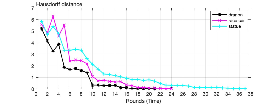
Figure 20. Shapes with tens of thousands of FLSs, $\epsilon$=5$\degree$, M=$\infty$.

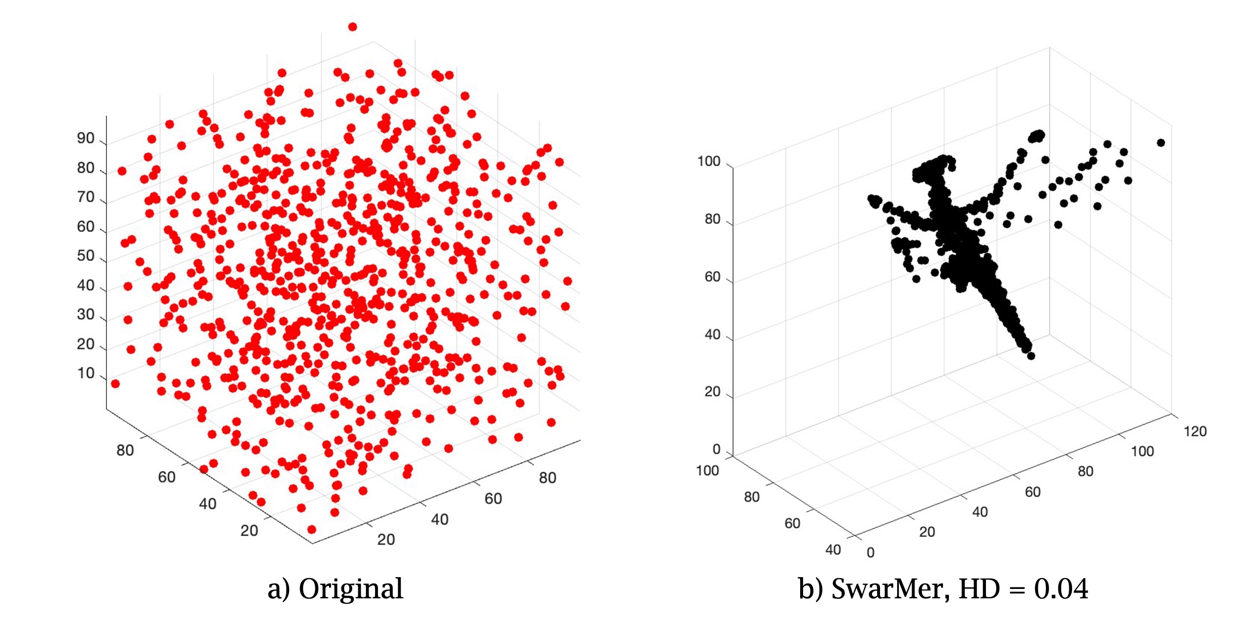
Figure 21. Random placement, see https://youtu.be/cZrz0e61txU.

4.2.4. Random FLS placement

SwarMer will work with a random placement of FLSs in a 3D display as long as the coordinates of a point are assigned to each FLS. A limitation is that the shape may be shifted along the different axes by a wide margin because SwarMer is a relative localization technique. The precise amount of shift depends on how FLSs form swarms, and how swarms merge and move. To illustrate, consider the 3D dragon of Figure 13. We assign FLSs to a 3D space using a random number generator, see Figure 21.a. FLSs use SwarMer to localize and render the dragon with a Hausdorff distance less than 0.09 in 26 rounds, see Figure 21.b. The dragon is shifted along the different axes. One may address this limitation by having either a reference point on the display with a well known position or an oracle FLS configured with specialized hardware that computes its position with a high accuracy. A swarm that localizes relative to either inherits the oracle property. All other swarms are required to localize relative to its FLSs, preventing a shape from shifting across different axes.

5. A Comparison

In our first approach to localize FLSs to render shapes, we considered the feasibility of using triangulation and trilateration. We hypothesized that using those FLSs with a high confidence in their location as anchors will produce shapes with a high accuracy. This hypothesis proved wrong because trilateration and triangulation compound small errors in anchor locations to produce distorted shapes. Below, we describe how an FLS computes its confidence. Subsequently, we describe triangulation and trilateration in turn. This section ends with a comparison of these techniques with SwarMer.

Confidence: Once an FLS $i$ ($F_{i}$) arrives at its destination, it may compute its confidence $C_{i}$ using either the average or worst estimated error attributed to dead-reckoning. With average (worst), it computes the average (maximum) radius R around the semi-circle in 2D (semi-sphere in 3D) as the error in its position relative to each of its $n_{i}$ neighbors. Its confidence is defined as:

(1) $$C_{i}=1-\sum_{k=1}^{n_{i}}{min(\frac{1}{n_{i}},\frac{R}{\delta_{gt}(F_{i},F_{k})})}$$

where $\delta_{gt}(F_{i},F_{k})$ is the distance between FLS $i$ and a neighboring FLS $k$ in the ground truth. When a neighbor is missing, $R$ is set to a large value, e.g., max integer. This causes Equation 1 to use $\frac{1}{n_{i}}$ for the missing neighbor. A large value of $C_{i}$ means the FLS’s estimated truth reflects the ground truth more accurately. $C_{i}$ equal to 1.0 is ideal.

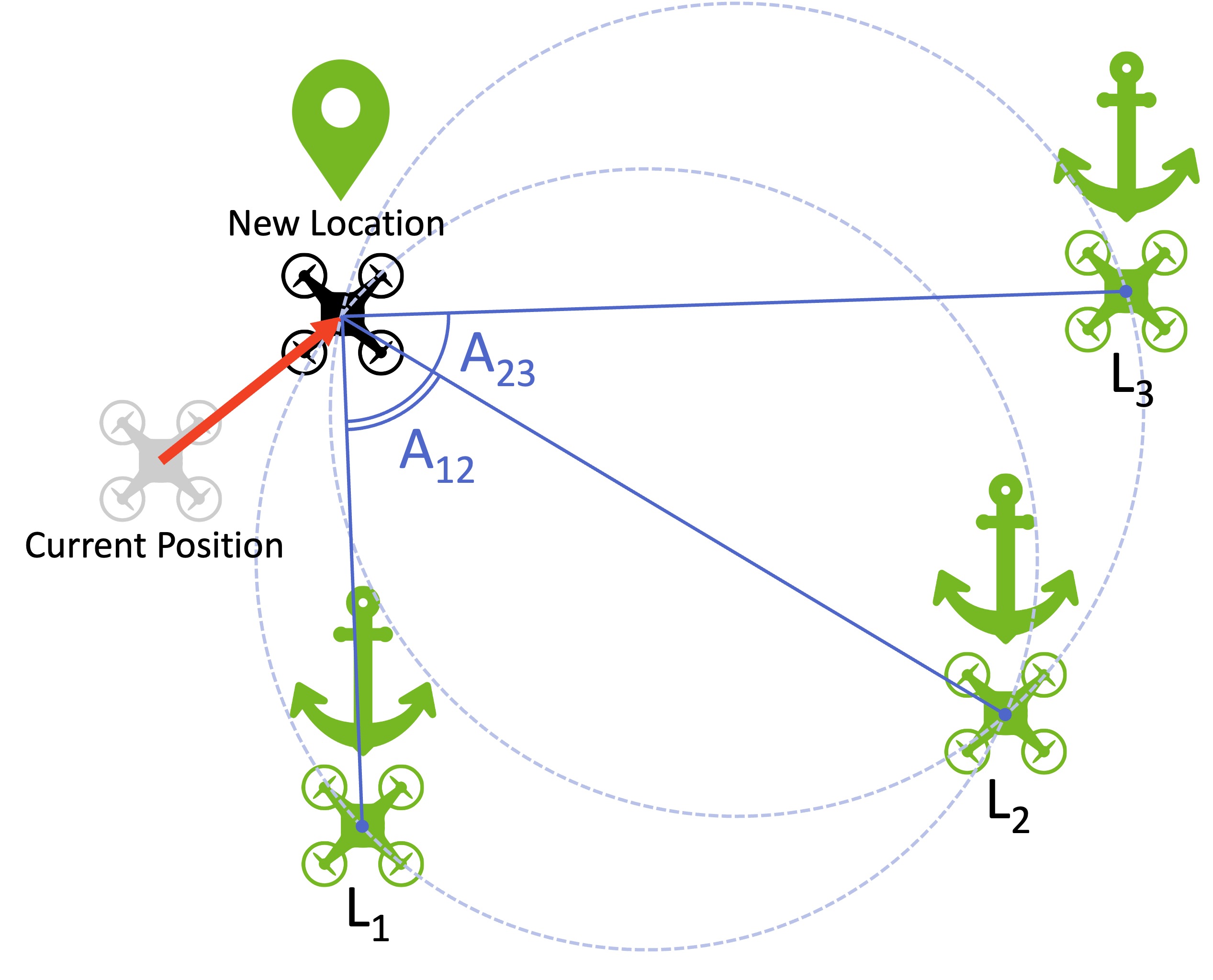
Figure 22. Triangulation

Three Object Triangulation requires a localizing object to compute its location and orientation using its angles relative to three objects. Alternative techniques include iterative search, geometric circle intersection, and Newton-Raphson iterative method (Cohen and Koss, 1993). We use the geometric circle intersection method since it is widely used in the literature and ranked as the best when compared with the other two techniques (Cohen and Koss, 1993).

The geometric circle intersection method is fast and its failures are easy to detect. It requires a localizing FLS, the one with the lowest confidence relative to its neighbors, to compute two circles using the estimated location and the ground truth angle of three FLSs. See Algorithm 1 and Figure 22. The three FLSs may be its neighboring FLSs. In most cases, the two circles intersect at two points. These points are the mutual FLSs and the location of the localizing FLS. The latter has an angle relative to the other three FLSs in the ground-truth. If these angles match those in the estimated truth then the localizing FLS does not move. Otherwise, the localizing FLS computes a new location for itself that matches the angles in the ground truth. The localizing FLS flies to this new location.

1 $f\leftarrow FLS~{}with~{}the~{}lowest~{}confidence~{}in~{}its~{}location$;

2 $\{L\}=3~{}randomly~{}selected~{}neighbors~{}of~{}f$ $\triangleright$ *[r]Return error if F has fewer than 3 neighbors $\{A_{12},A_{23}\}=angles~{}of~{}f~{}to~{}\{L\}~{}in~{}the~{}ground~{}truth,Figure~{}\ref{fig:triangulation}$;

3 $Compute~{}estimated~{}location~{}of~{}\{L\}~{}in~{}the~{}estimate~{}truth$;

4 $Compute~{}a~{}new~{}location~{}for~{}f~{}such~{}that~{}its~{}angle~{}to~{}\{L\}~{}in~{}$
$the~{}estimated~{}truth~{}is~{}the~{}same~{}as~{}the~{}ground~{}truth$;

5 $Move~{}f~{}to~{}the~{}location~{}computed~{}in~{}Step~{}5$;

$Repeat~{}the~{}above~{}6~{}steps~{}until~{}each~{}FLS’s~{}confidence~{}exceeds$
$~{}a~{}prespecified~{}threshold$

Algorithm 1 Triangulation, Circle Intersection Method

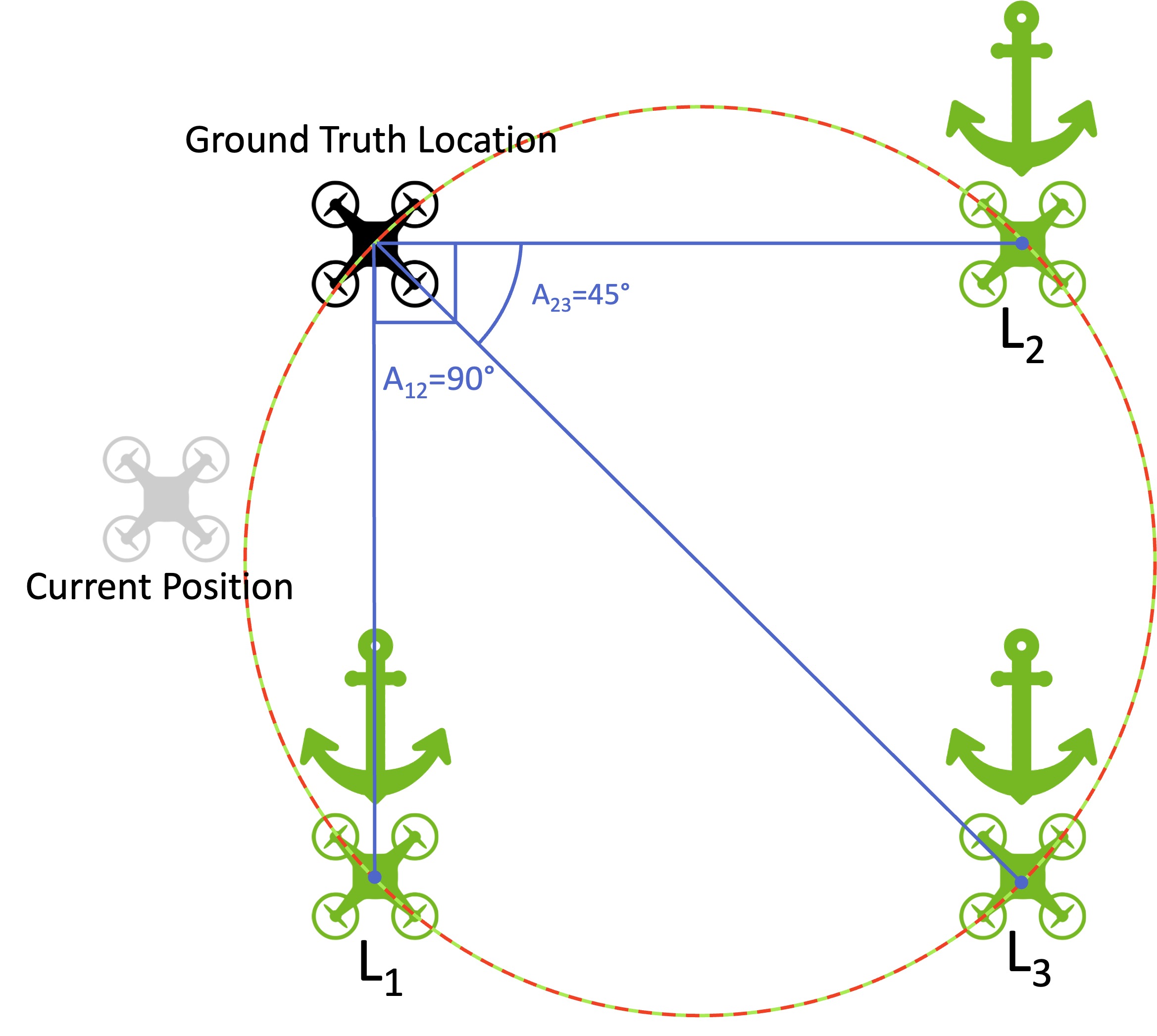
Figure 23. Failure of Triangulation.

This method fails when the center of the two circles is too close (we used 1 illumination cell) or when two circles overlap, see Figure 23.

Figure 24. Trilateration

Three Object Trilateration is the use of distances or ranges for determining the unknown location of an object. The localizing FLS $i$ computes its distance to three neighboring FLSs in the ground truth: $D_{1}$, $D_{2}$, and $D_{3}$. See Figure 24. Each delta is the radius of a circle with the corresponding neighbor as its center. FLS $i$ computes a new estimated location that matches $D_{1}$, $D_{2}$, and $D_{3}$ in its estimated truth. This is the new location of FLS $i$.

Trilateration fails when either the three circles do not intersect at the same point in the ground truth, or there is no location in estimated truth that matches $D_{1}$, $D_{2}$, and $D_{3}$. While rare, both do occur in our experiments.

Our implementation of both triangulation and trilateration assumes Signal Strength (SS) measurements in the estimated truth match those of the ground truth with 100% accuracy. It also assumes an FLS is able to measure angle with triangulation and distances with trilateration with 100% accuracy. We made these assumptions because triangulation and trilateration perform poorly. We wanted to remove error in measuring angle and distance as a possible explanation for their inferior localization.

1 $f\leftarrow FLS~{}with~{}the~{}lowest~{}confidence~{}in~{}its~{}location$;

2 $\{L\}=3~{}randomly~{}selected~{}neighbors~{}of~{}f$ $\triangleright$ *[r]Return error if F has fewer than 3 neighbors $\{D\}=distance~{}of~{}f~{}to~{}\{L\}~{}in~{}the~{}ground~{}truth,Figure~{}\ref{fig:trilateration}$;

3 $Compute~{}location~{}of~{}\{L\}~{}in~{}the~{}estimated~{}truth$;

4 $Compute~{}a~{}new~{}location~{}for~{}f~{}such~{}that~{}its~{}distance~{}to~{}\{L\}~{}in~{}$
$the~{}estimated~{}truth~{}is~{}the~{}same~{}as~{}the~{}ground~{}truth$;

5 $Move~{}f~{}to~{}the~{}location~{}computed~{}in~{}Step~{}5$;

$Repeat~{}the~{}above~{}6~{}steps~{}until~{}each~{}FLS’s~{}confidence~{}exceeds$
$~{}a~{}prespecified~{}threshold$

Algorithm 2 Trilateration

5.1. Experimental Results

Figure 25.a-d show rendering of a 2D butterfly using dead reckoning with different degrees of error, $\epsilon$=$\{1\degree,3\degree,5\degree\}$. Figure 25.b shows application of SwarMer to each butterfly. It continues to use the same $\epsilon$ when applying dead reckoning using signal strength. The last two rows of Figure 25 show triangulation and trilateration do not improve the quality of illumination. With both, an FLS uses the worst estimated error attributed to dead-reckoning to compute its confidence. Trilateration decreases the quality of rendering when compared with dead reckoning with $\epsilon$=1$\degree$. This is despite the fact that both triangulation and trilateration are provided with 100% accurate angle and distance measurements using signal strength. Similar results are observed with the cat and the teapot in Figure 1. The key difference is that Figure 1 reports results with $\epsilon$=5$\degree$ while Figure 1 shows different degrees of error, $\epsilon$=$\{1\degree,3\degree,5\degree\}$.

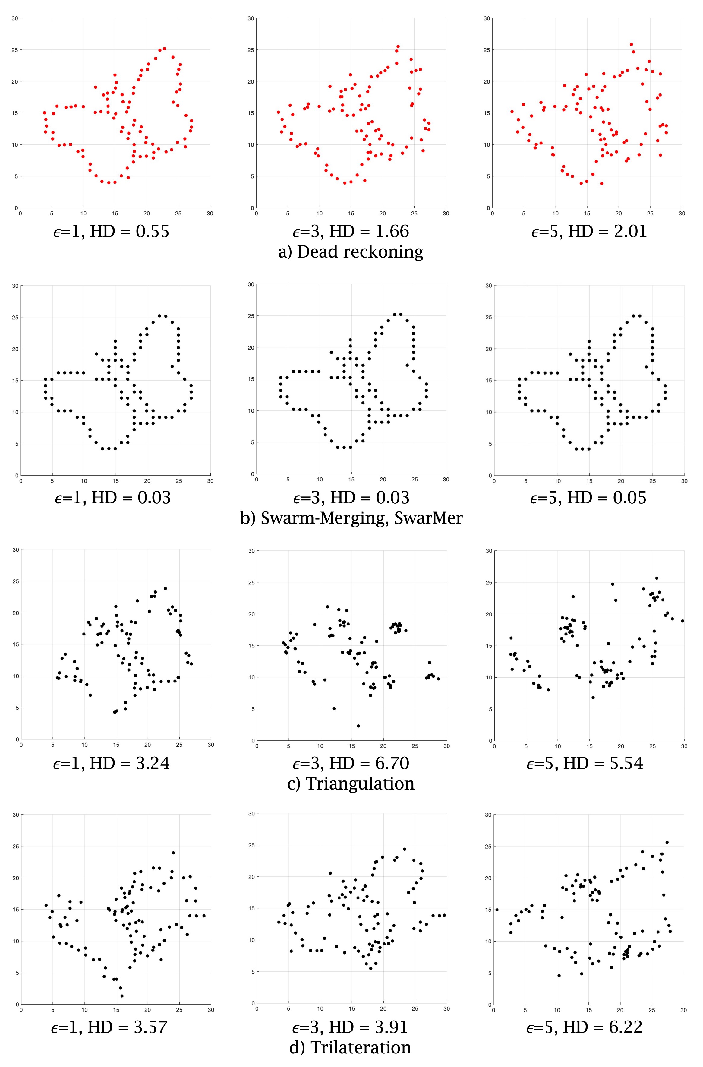
Figure 25. (a) A 2D butterfly with dead reckoning and three different degrees of error, (b) with SwarMer, (c) with Triangulation, and (d) Trilateration.

The number of points in a point cloud impacts the quality of renderings with small values of $\epsilon$. Figure 26 shows a 2D butterfly consisting of 1008 points, more than ten times the number of points in the butterfuly of Figure 25. The FLSs deployed from the origin, (0,0), travel the longest distance to the rightmost wing of the butterfly, incurring the highest amount of error and the most distortion with $\epsilon$=5$\degree$. With $\epsilon$=1$\degree$, the shape of the butterfly is recognizable with both triangulation and trilateration. However, their Hausdorff distance is worse than dead reckoning by itself. With $\epsilon$=3 and 5 degrees, triangulation results in a few FLSs to move away from the illumination by a large distance. This is reflected in their longer scale of the x-axis in Figures 26c. While trilateration does not suffer from this limitation, its localization results in distorted shapes with a large Hausdorff distance. SwarMer continues to provide accurate localization subjectively, see Figures 26b. It realizes a Hausdorff distance lower than 0.09 by executing 20, 30, and 40 rounds with $\epsilon$=1, 3, and 5 degrees, respectively.

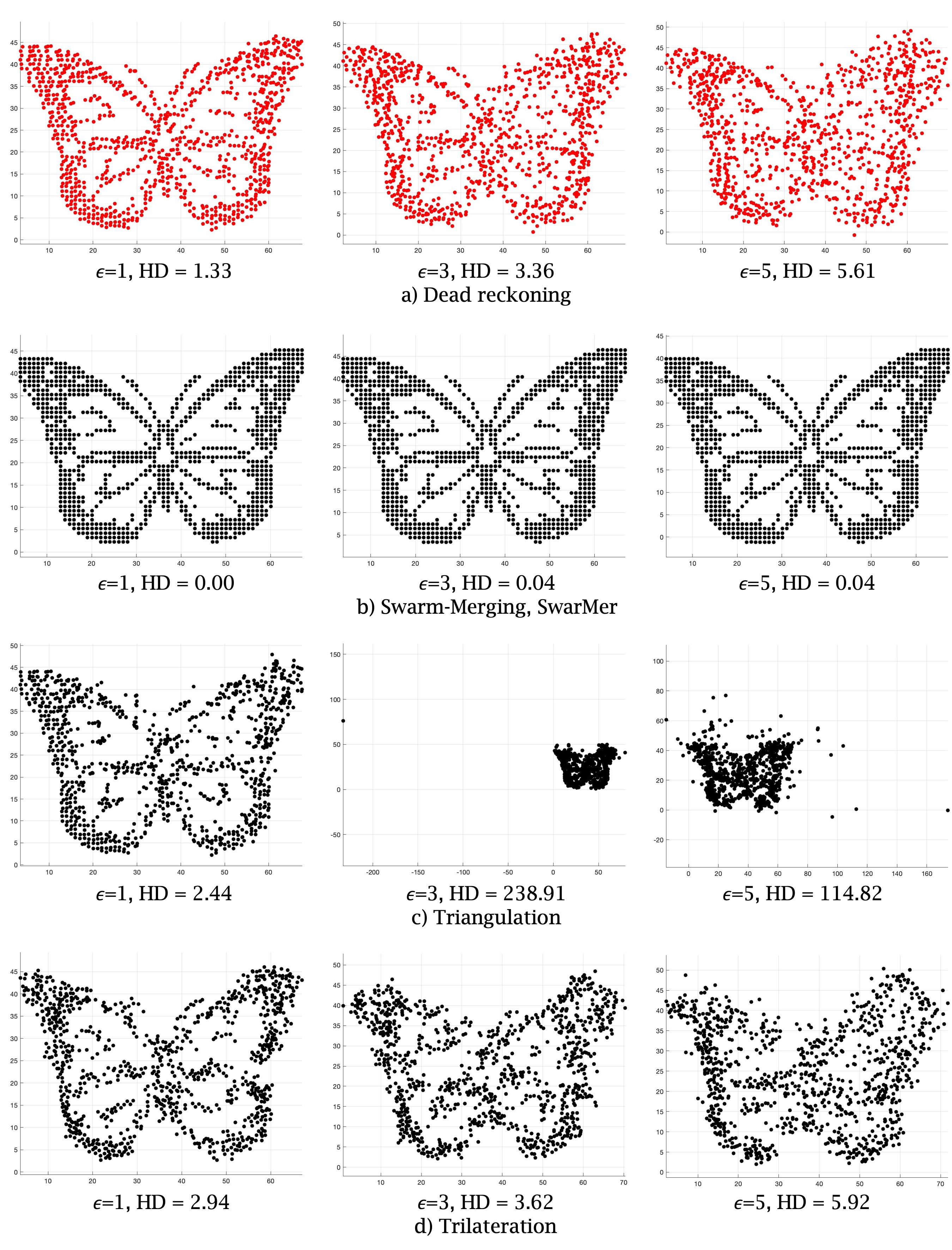
Figure 26. (a) A 2D butterfly with dead reckoning and three different degrees of error, (b) with SwarMer, (c) with Triangulation, and (d) Trilateration..

6. An Implementation

We implemented SwarMer as a process to execute on board an FLS. Processes exchange messages to implement SwarMer. Our current implementation uses the Python 3.9 programming language. We used a cluster of Amazon AWS instance u-6tb1.112xlarge to conduct the experiments reported in this section. Each instance consists of 448 virtual cores and 6 Terabytes of memory. While the Dragon requires a cluster of 6 such servers, the Hat and the Skateboard use a cluster of 16 such servers because they consist of more points (FLSs).

Each process is termed $P_{FLS}$ and implements a finite state machine that maintains the following 5 states: Deploying, Available, Busy Anchor, Busy Localizing, and Waiting. 11 events corresponding to different message types transition the state of a $P_{FLS}$ to implement SwarMer.

A $P_{FLS}$ consists of two threads: A networking thread ($T_{Network}$) and a handler thread ($T_{Handler}$) that mutates the state of the machine. While $T_{Network}$ only reads the FLS state, $T_{Handler}$ may read and write the FLS state. $T_{Network}$ blocks on the network socket and processes messages as fast as they arrive by reading the current state of the machine. One of its objectives is to release the lease granted to an FLS that has decided to become an anchor FLS itself. In addition, it is designed to minimize latency between cooperating FLSs, expediting the execution of SwarMer to form shapes faster. $T_{Network}$ places those messages that change system state in a queue for processing by $T_{Handler}$. $T_{Handler}$ consumes these messages from the queue and may transition and update the state of the machine. The queue introduces delays and $T_{Network}$’s processing of certain messages minimizes the impact of this delay on a swarm of cooperating FLSs.

This implementation is different from the Matlab simulation model in several ways. First, each $P_{FLS}$ implements the concept of time by either sleeping or busy-waiting for the duration of time it travels from its current location to a new destination. It has a realistic velocity model that controls its acceleration and deceleration to arrive at its destination with a speed of zero. Second, each $P_{FLS}$ implements a UDP-Wrapper that emulates a networking card with an adjustable radio range. The time required for a $P_{FLS}$ to expand its radio range and transmit messages is another difference from the Matlab simulator. Third, a $P_{FLS}$ may incur different forms of failures such as packet loss, and a process shutdown to simulate FLS failures. Finally, a $P_{FLS}$ uses a probabilistic method to thaw the final swarm. With this method, a $P_{FLS}$ sets a timer to expire between $H$ and $2H$ seconds where $H=log_{2}F$ and F is the number of FLSs. Once an FLS’s timer expires, it broadcasts a thaw message using its maximum radio range. A receiving FLS sets its Swarm-ID to its FID and resets its timer.

The lessons learned from the emulator are as follows:

• Within a few seconds, SwarMer reduces the HD by several orders of magnitude.

• Packet loss as high as 10% does not hinder SwarMer’s ability to reduce the HD in the first few seconds. It is able to construct a single swarm in the presence of packet loss.

• Today’s small drones may travel at speeds as fast as 3 to 5 meters/second. While FLS speed impacts the initial deployment of FLSs using dead reckoning, it does not impact how fast SwarMer improves the quality of an illumination (i.e., drop in HD) as a function of time. The key insight is that the average distance moved by an FLS (or swarm) to localize is small. This prevents an FLS from accelerating to its maximum speed.

• SwarMer is resilient to FLS failures. It incorporates FLSs that replace failed FLSs seamlessly.

• FLS latency in processing messages may result in undesirable race conditions that slow-down SwarMer without impacting its functionality. We present a multi-threaded $P_{FLS}$ to minimize processing latency.

In our experiments with drones, we have observed the communication link to drop packets. A $P_{FLS}$ uses UDP (instead of TCP) to communicate with other $P_{FLS}$s. UDP is an unreliable communication protocol. It may drop packets, deliver a sequence of packets transmitted by a $P_{FLS}$ out of order, and delay the delivery of packets. Our implementation of SwarMer is non-blocking to accommodate the first two features of UDP. With UDP’s last two features, we introduced a monotonically increasing message id for each packet sent by a $P_{FLS}$. A $P_{FLS_{j}}$ maintains the largest message id it has received from another $P_{FLS}$ and may drop those with a smaller id.

A transmitting $P_{FLS}$ uses UDP in broadcast mode. The emulated processes run on one or more servers. A message sent by one process is received by all processes. We built a thin networking layer around UDP, a UDP-Wrapper, to implement an adjustable radio range. The UDP-Wrapper implements a networking card with a fixed radio range. It uses the distance between FLSs in the ground truth to decide whether a $P_{FLS}$ receives a UDP message broadcasted by another $P_{FLS}$. When a process (i.e., an FLS) broadcasts a message within a fixed radio range, only the processes (FLSs) in this radio range receive the message.

Pushing features into the UDP-Wrapper expedites the processes on a multi-core server. For example, when a member of the swarm issues the challenge message, all FLS processes in the same swarm receive the message due to the broadcast nature of UDP. The UDP-Wrapper may compare the Swarm-ID of a process with the Swarm-ID of the challenger (embedded in the message), dropping the packet with a matching Swarm-ID. Such optimizations enhance performance and reduce the variation in the duration of time required to form a single swarm.

$\lambda$	Total Xmit bytes	# Localizations	# Anchor	# Thawed swarms	# Leases expired	Avg distance traveled
50 ms	706,152,707	41,814	39,569	1,507,271	8606 (11.03%)	70.38
200 ms	284,105,583	15,218	16,131	468,330	2468 (6.92%)	68.37
300 ms	381,641,949	21,050	22,279	830,543	3351 (6.78%)	69.92
450 ms	235,055,229	12,582	13,511	553,477	2013 (6.53%)	72.68
700 ms	153,765,307	8,406	9,149	335,810	1158 (5.35%)	74.67
1000 ms	102,582,418	5,427	5,892	170,807	746 (5.16%)	75.24

Table 2. System metrics as a function of $\lambda$ for a two minute execution of SwarMer.

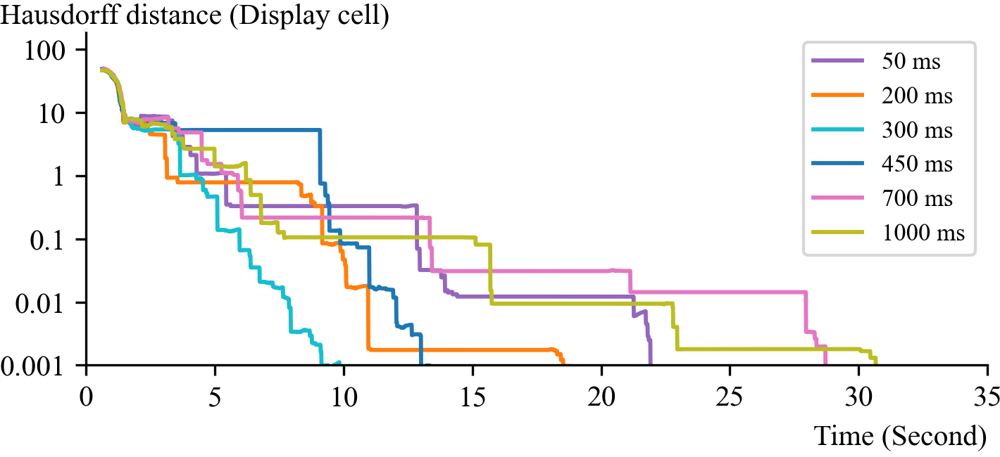
Figure 27. HD with different challenge inter-arrival times, $\lambda$ for a 3D figure sampled with 200 points from the Chess piece. Video clips showing the illuminations with $\lambda$ values 50, 450, and 1500 msec intervals available at https://youtu.be/zwTUgKvg6sI, https://youtu.be/AKJFu05eM1Y, and https://youtu.be/8_OtMU4bE74, respectively.

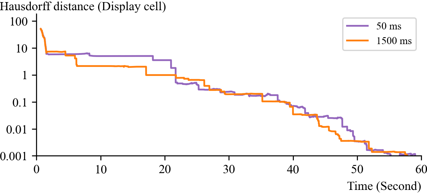
Figure 28. HD with different challenge inter-arrival times, $\lambda$ for the Skateboard. Video clips with $\lambda$ values 50 and 450 available at https://youtu.be/WdjsTJp1RNY and https://youtu.be/pzaOrDuvL3g, respectively.

A key parameter of SwarMer is the inter-arrival time $\lambda$ between the Challenge messages issued by $T_{Handler}$ thread of an FLS to its neighbors. Figure 30 shows the HD with the different values of $\lambda$. Table 2 shows key system metrics for different $\lambda$ values. Experiments below use $\lambda$=500 msec.

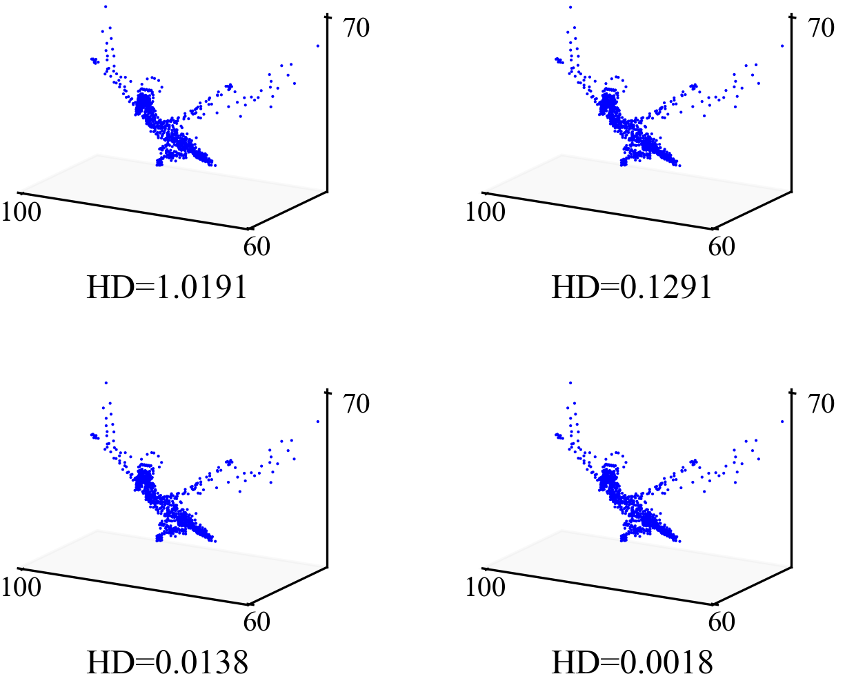
(a) Dragon, https://youtu.be/PRyjdmw8NVc

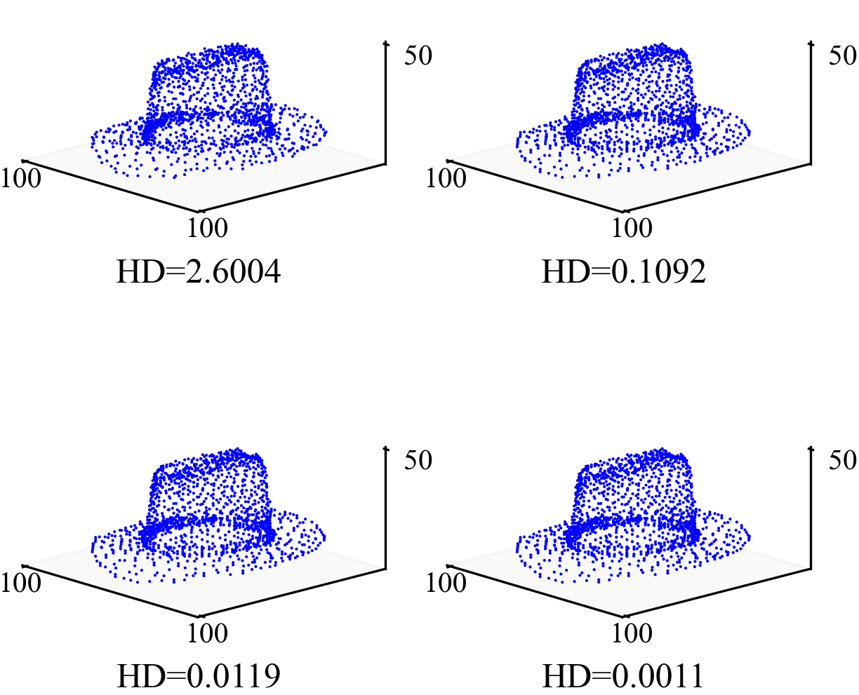
(b) Hat, https://youtu.be/y_xHdz5bs5M

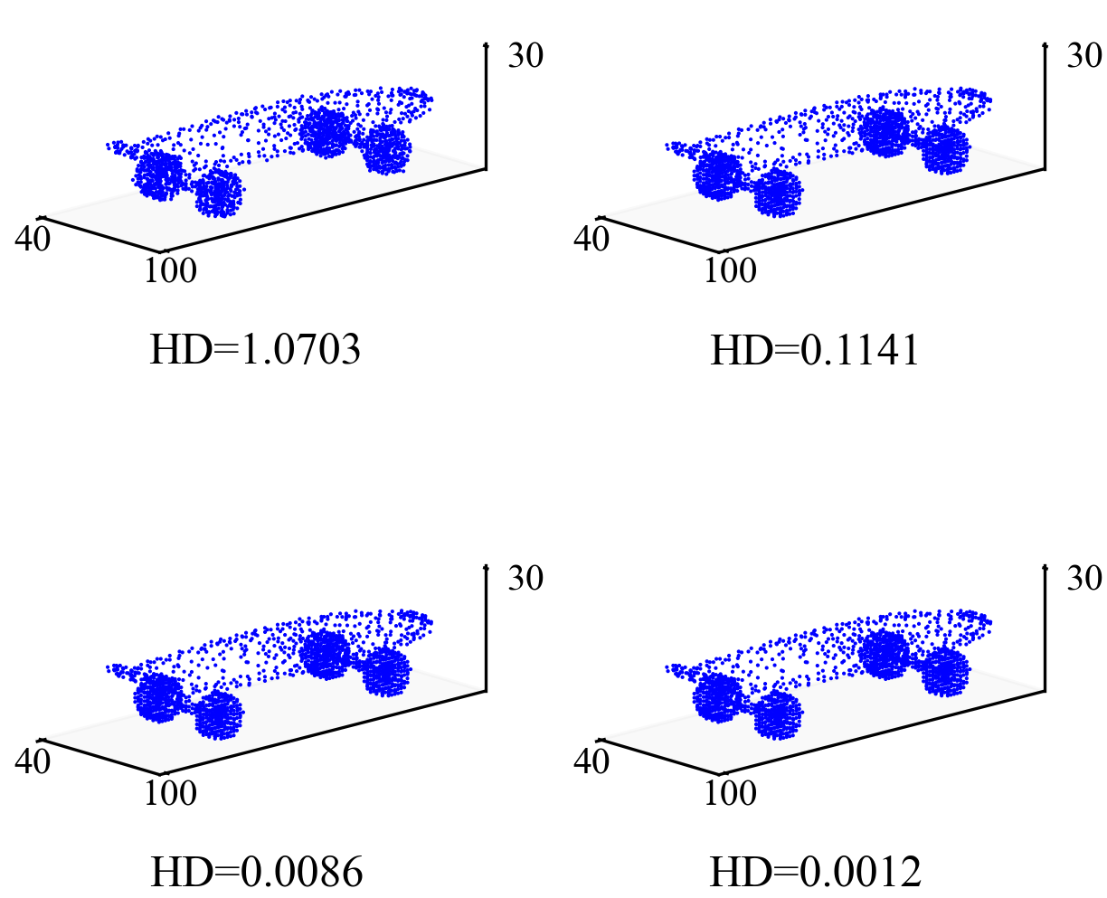
(c) Skateboard, https://youtu.be/a0fFu0z6BU0

Figure 29. No FLS movement is visible with HD$<$0.1. Click the URLs for a video.

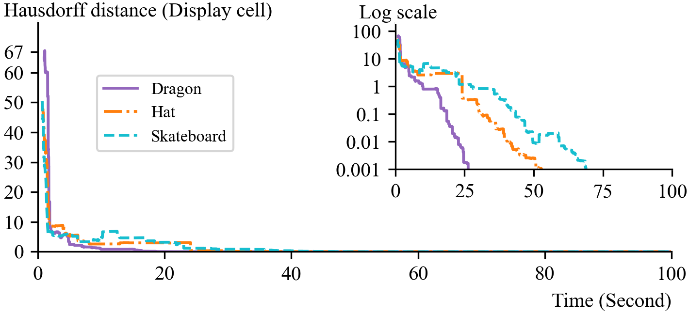
Figure 30. HD with 3D shapes of Figure 12, $\epsilon$=5$\degree$. The figure inside shows the HD in log scale.

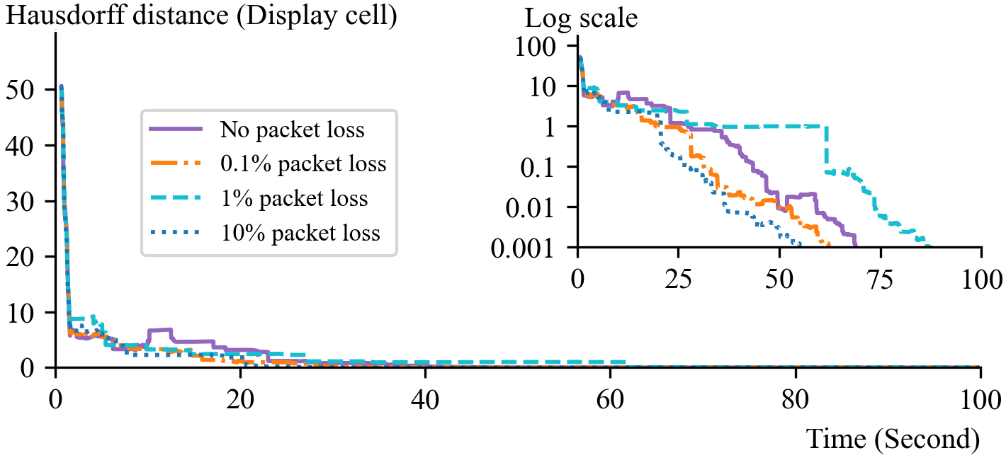
(a) Packet loss at receiver $P_{FLS}$. The figure inside shows the HD in log scale.

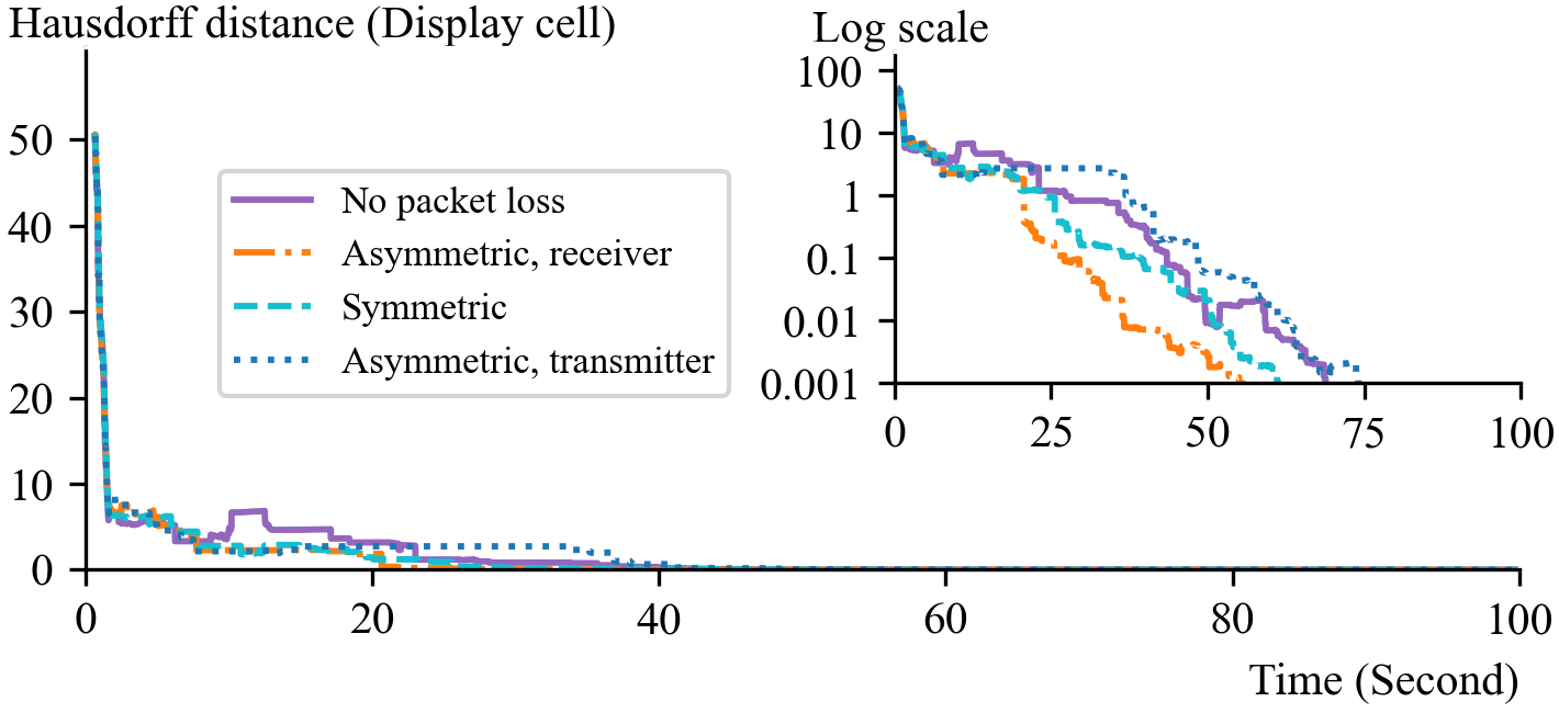
(b) 10% packet loss. The figure inside shows the HD in log scale.

Figure 31. HD with packet loss, Skateboard, $\epsilon$=5$\degree$.

Obtained Results. Figure 30 shows the HD as a function of time for the different shapes in Figure 12. The y-axis of this figure is linear scale. It reports HD as a function of the length of a display cell, a cube with a 5 Centimeter length. Hence, a HD of 1 means the maximum distance between the points in the ground truth and the estimated truth is 5 Centimeter. HD drops significantly in the first few seconds of SwarMer’s execution because FLSs localize relative to one another. When this distance drops below 50 Micrometer (0.005 Centimeter corresponding to HD of 0.001), we consider it close to zero and stop reporting the distance. The different shapes arrive at this threshold at different times. See the variant of the Figure inside its empty space with y-axis in log scale. The Dragon arrives at this threshold soonest as it consists of 760 FLSs. The Skateboard requires the longest as it consists of more than twice (1727) as many FLSs.

Figure 29 shows the different shapes with HD values of 1, 0.1, and two HD values below 0.1. There is no noticeable difference between the shapes with HD values lower than 0.1, i.e., a 5 millimeter error.

We designed the UDP-Wrapper to support both symmetric and asymmetric packet loss. It may be configured to drop packets with a pre-specified probability either at the transmitting, receiving, or both. Figure 31 shows SwarMer is resilient to all kinds of network errors for the Skateboard. Depending on which event is lost, SwarMer may require a longer time to construct one swarm. However, it continues to decrease the HD dramatically in the first few seconds of its execution. We present the Skateboard because its reported HD for different forms of packet loss and loss rates are farthest apart, see the log scale version of the graph in Figure 31. They are alot closer for the Dragon and the Hat.

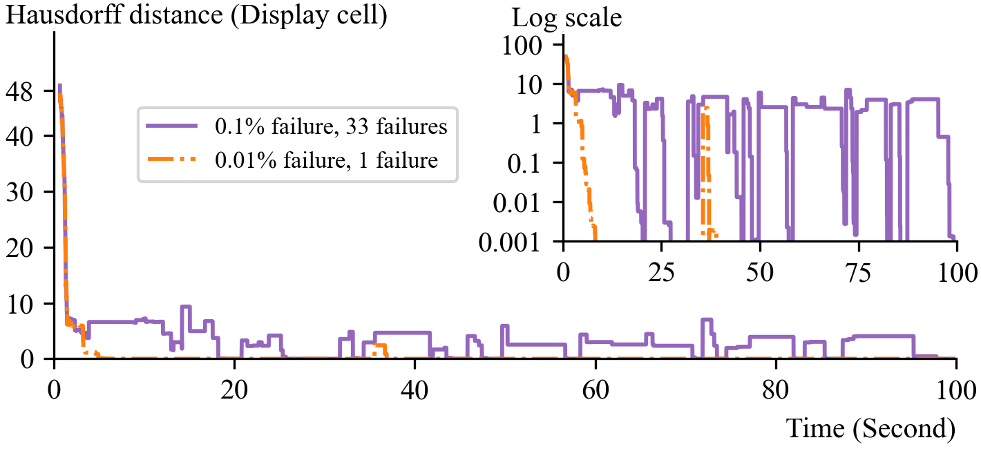
Figure 32. HD with 0.1% and 0.01% failures per FLS per second for a 3D figure sampled with 200 points from the Chess piece.

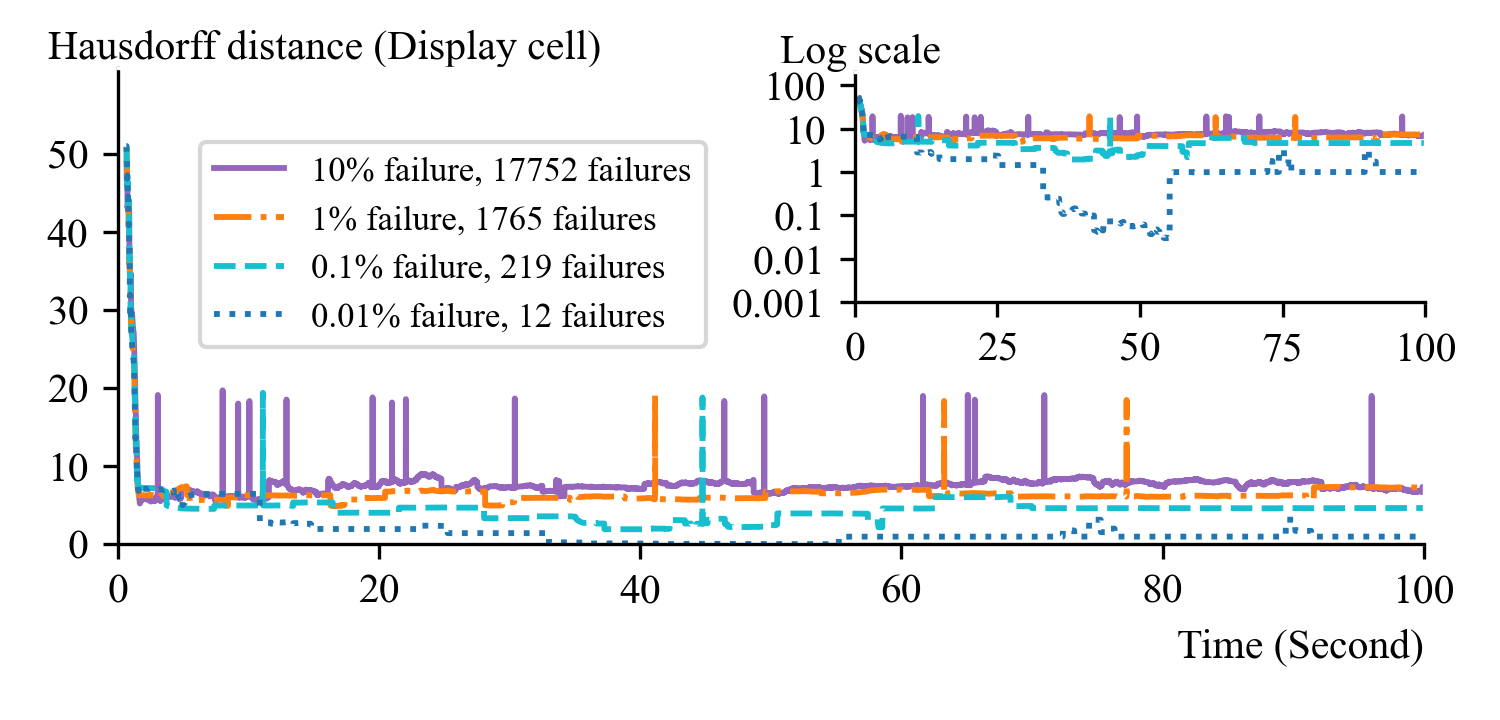
Figure 33. HD with 0.01%, 0.1%, 1%, and 10% failures per FLS per second for the Skateboard. Video clips available at https://youtu.be/YE-hzpfONwg, https://youtu.be/1Tx-_DDZf0w, https://youtu.be/QEKJgNn0Yy8, https://youtu.be/mU-oIVaNu8M, respectively.

SwarMer’s use of leases enables it to tolerate FLS failures. A replacement FLS deployed by a dispatcher may execute SwarMer to incorporate itself. Figure 32 shows the HD with two different probabilities of failure per second per FLS: 0.1% and 0.01%. The HD is different with 0.1% and 0.01% failures per second per FLS because there are a total of 33 and 1 failures during a 100 second execution of SwarMer. The failure of an FLS causes a point to go dark. A dispatcher deploys its replacement FLS. Once this FLS arrives at its coordinates using dead reckoning, it illuminates its assigned point. This causes the HD to increase. As the FLS localizes and merges into the swarm, the HD decreases. This is shown as the sharp drop with the 0.01$ failure. There are more failures with 0.1%. The swarm is thawed when either all FLSs form one swarm or a fixed amount of time elapses. This time is log (base 2) of the number of points, approximately 8 seconds in Figure 32. When a replacement FLS arrives at its coordinates, it may have to localize itself several times to reduce the HD. Each time, this FLS must wait for the swarm to thaw. This explains the plateaus in the order of seconds in Figure 32.

SwarMer is not a failure handling technique. With a high failure rate, the resulting HD may be high. Figure 33 shows the HD with the Skateboard and failure rates as high as 10%. The HD is high with a failure rate of 1% and higher because SwarMer incorporates many replacement FLSs concurrently. The respective video clips show a distorted image. The display requires standby FLSs (Ghandeharizadeh, 2022) to maintain a high quality of illumination.

7. Related Work

The SwarMer framework to localize FLSs is novel and to the best of our knowledge has not been described elsewhere.

Outdoor drone shows use GPS (Samama, 2008) to localize and illuminate shapes in the sky. The largest show consisted of 5200 drones to celebrate the 100th anniversary of the Communist Party of China in the night sky of Longgang, Shenzhen. An FLS display is different because it does not have line of sight with GPS satellites.

The concept of a 3D display using FLSs to render multimedia shapes (Ghandeharizadeh, 2021, 2022; Alimohammadzadeh et al., 2023b; Phan et al., 2023; Alimohammadzadeh et al., 2023a) is relatively new. Prior studies either identify localization as a challenge (Ghandeharizadeh, 2021; Alimohammadzadeh et al., 2023a; Phan et al., 2023) or assume one without describing it (Ghandeharizadeh, 2022; Alimohammadzadeh et al., 2023b). SwarMer is novel and designed for use by these studies.

Centralized indoor techniques such as optical motion capture systems merge images from fixed cameras positioned around a display volume to localize quadrotors and drones (Kushleyev et al., 2013; Ritz et al., 2012; Preiss et al., 2017b). These systems, e.g., Vicon, are highly accurate. They require a unique marker arrangement for each drone and have enabled control and navigation of swarms of tens of drones. It may be difficult (if not impossible) to form unique markers for more than tens of small drones measuring tens of millimeters diagonally (Preiss et al., 2017b). Hence their scalability is limited. Moreover, these systems require broadcast at high frequency from a central computer to each drone (Weinstein et al., 2018). This centralized communication channel is a single point of system failure. It has a latency of several (7) milliseconds (Preiss et al., 2017b) and its bandwidth constrains the robustness and swarm size. SwarMer is different because it is decentralized, requiring each FLS to localize relative to its neighbor to form a swarm. The broadcast range of an FLS is controlled by its signal strength to communicate with a fixed number ($\eta$) of neighboring FLSs.

There exists a large number of studies in the area of formation control (Tron et al., 2016; Zhao et al., 2019; Van Tran and Ahn, 2020; Chan et al., 2021), use of sensors to localize robots and drones (Ledergerber et al., 2015; Alarifi et al., 2016; Zhiqiang et al., 2021; Großiwindhager et al., 2019; Klein and Murray, 2007; Engel et al., 2018; Klose et al., 2010; Babinec et al., 2014; Xu et al., 2020, 2022; Xiao et al., 2023; Xie et al., 2018; Mur-Artal and Tardós, 2017; Qin et al., 2018; Geneva et al., 2020; Dube et al., 2017; Zhang and Singh, 2014; Wang et al., 2021a; Lin and Zhang, 2020; Kao et al., 2023; Yang et al., 2021; Nguyen et al., 2021), and collision avoidance (Guy et al., 2009; Augugliaro et al., 2012; Chen et al., 2015; Hamer et al., 2018; van den Berg et al., 2008, 2011a, 2011b; Stephan et al., 2013; van den Berg et al., 2012; Bareiss and van den Berg, 2013; Arul and Manocha, 2020; Engelhardt et al., 2016; Cheng et al., 2017; Morgan et al., 2013; Báča et al., 2018; Morgan et al., 2014; Tabasso et al., 2021; Cappello et al., 2020; Mylvaganam et al., 2017; Preiss et al., 2017b; Ferrera et al., 2018; Xu et al., 2019; Preiss et al., 2017a; Kushleyev et al., 2013; Jiang et al., 2014). These studies complement SwarMer and may be used by a system that implements a 3D display (Alimohammadzadeh et al., 2023a). These prior studies lack the concept of FLSs forming a group (swarm), requiring a swarm to move together, swarms merging to become one, FLSs thawing their membership to repeat the process continuously, or use leases to explicitly support FLSs failing and leaving to charge their batteries. These concepts, their decentralized design and implementation are novel and a contribution of SwarMer.

8. Conclusions and Future Research

Inspired by swarms in nature, SwarMer is a decentralized technique for relative localization of FLSs to render complex 2D and 3D shapes. It requires FLSs to localize relative to one another to form a swarm. Movement of an FLS along a vector causes its entire swarm to move along the vector. SwarMer uses the unique identifier of an FLS assigned at its deployment time to implement an organizational framework. This framework compensates for the simplicity of individual FLSs to render complex 2D and 3D shapes accurately.

We presented a MATLAB simulation and a Python implementation of SwarMer. The implementation shows SwarMer is fast. Within a few seconds, it reduces the HD to a value below 1 display cell. Its continued execution reduces the HD further to match the ground truth more accurately. It tolerates network packet loss, FLSs failing and leaving to charge their battery, and FLSs returning to illuminate points.

We are initiating an implementation of SwarMer by evaluating the relevant plugins to the SwarMer. These include an investigation of the formation control techniques, alternative sensors for a localizing FLS to orient itself relative to an anchor FLS, and a collision avoidance technique as an FLS moves along a vector, see Section 7.

9. Acknowledgments

We thank Jiadong Bai and Shuqin Zhu for their valuable comments on the earlier drafts of this paper. This research was supported in part by the NSF grant IIS-2232382. We gratefully acknowledge CloudBank (Norman et al., 2021) and CloudLab (White et al., 2002) for the use of their resources to enable all experimental results presented in this paper.

References

- (1)
- Alarifi et al. (2016) Abdulrahman Alarifi, AbdulMalik Al-Salman, Mansour Alsaleh, Ahmad Alnafessah, Suheer Al-Hadhrami, Mai A. Al-Ammar, and Hend S. Al-Khalifa. 2016. Ultra Wideband Indoor Positioning Technologies: Analysis and Recent Advances. Sensors 16, 5 (2016). https://doi.org/10.3390/s16050707
- Alimohammadzadeh et al. (2023a) Hamed Alimohammadzadeh, Rohit Bernard, Yang Chen, Trung Phan, Prashant Singh, Shuqin Zhu, Heather Culbertson, and Shahram Ghandeharizadeh. 2023a. Dronevision: An Experimental 3D Testbed for Flying Light Specks, arXiv, 2308.10121. https://arxiv.org/abs/2308.10121. arXiv:2308.10121 [cs.MM]
- Alimohammadzadeh et al. (2023b) Hamed Alimohammadzadeh, Daryon Mehraban, and Shahram Ghandeharizadeh. 2023b. Modeling Illumination Data with Flying Light Specks. In ACM Multimedia Systems (Vancouver, Canada) (MMSys ’23). Association for Computing Machinery, New York, NY, USA, 363–368. https://doi.org/10.1145/3587819.3592544
- Arul and Manocha (2020) Senthil Hariharan Arul and D. Manocha. 2020. DCAD: Decentralized Collision Avoidance With Dynamics Constraints for Agile Quadrotor Swarms. IEEE Robotics and Automation Letters 5 (2020), 1191–1198. https://doi.org/10.1109/LRA.2020.2967281
- Augugliaro et al. (2012) Federico Augugliaro, Angela Schoellig, and Raffaello D’Andrea. 2012. Generation of Collision-Free Trajectories for a Quadrocopter Fleet: A Sequential Convex Programming Approach. In Proceedings of the IEEE/RSJ International Conference on Intelligent Robots and Systems. IEEE/RSJ International Conference on Intelligent Robots and Systems. 1917–1922. https://doi.org/10.1109/IROS.2012.6385823
- Babinec et al. (2014) Andrej Babinec, Ladislav Jurišica, Peter Hubinský, and František Duchoň. 2014. Visual Localization of Mobile Robot Using Artificial Markers. Procedia Engineering 96 (2014), 1–9. https://doi.org/10.1016/j.proeng.2014.12.091 Modelling of Mechanical and Mechatronic Systems.
- Bareiss and van den Berg (2013) Daman Bareiss and Joran van den Berg. 2013. Reciprocal Collision Avoidance for Robots with Linear Dynamics using LQR-Obstacles. In Proceedings - IEEE International Conference on Robotics and Automation. 3847–3853. https://doi.org/10.1109/ICRA.2013.6631118
- Bawa et al. (2003) Mayank Bawa, Hector Garcia-Molina, Aristides Gionis, and Rajeev Motwani. 2003. Estimating Aggregates on a Peer-to-Peer Network. Technical Report 2003-24. Stanford InfoLab. http://ilpubs.stanford.edu:8090/586/
- Beinschob et al. (2017) Patric Beinschob, Mark Meyer, Christoph Reinke, Valerio Digani, Cristian Secchi, and Lorenzo Sabattini. 2017. Semi-automated map creation for fast deployment of AGV fleets in modern logistics. Robotics and Autonomous Systems 87 (2017), 281–295. https://doi.org/10.1016/j.robot.2016.10.018
- Bernardini et al. (2021) Fabio Bernardini, Alice Buffi, Daniele Fontanelli, David Macii, Valerio Magnago, Mirko Marracci, Andrea Motroni, Paolo Nepa, and Bernardo Tellini. 2021. Robot-Based Indoor Positioning of UHF-RFID Tags: The SAR Method With Multiple Trajectories. IEEE Transactions on Instrumentation and Measurement 70 (2021), 1–15. https://doi.org/10.1109/TIM.2020.3033728
- Báča et al. (2018) Tomáš Báča, Daniel Hert, Giuseppe Loianno, Martin Saska, and Vijay Kumar. 2018. Model Predictive Trajectory Tracking and Collision Avoidance for Reliable Outdoor Deployment of Unmanned Aerial Vehicles. In IEEE/RSJ International Conference on Intelligent Robots and Systems (IROS). 6753–6760. https://doi.org/10.1109/IROS.2018.8594266
- Campos et al. (2021) Carlos Campos, Richard Elvira, Juan J. Gómez Rodríguez, José M. M. Montiel, and Juan D. Tardós. 2021. ORB-SLAM3: An Accurate Open-Source Library for Visual, Visual–Inertial, and Multimap SLAM. IEEE Transactions on Robotics 37, 6 (2021), 1874–1890. https://doi.org/10.1109/TRO.2021.3075644
- Cano et al. (2022) Justin Cano, Gaël Pages, Eric Chaumette, and Jerome Le Ny. 2022. Optimal Localizability Criterion for Positioning with Distance-Deteriorated Relative Measurements. In 2022 IEEE/RSJ International Conference on Intelligent Robots and Systems (IROS). 947–953. https://doi.org/10.1109/IROS47612.2022.9981718
- Cappello et al. (2020) D. Cappello, S. Garcin, Z. Mao, M. Sassano, A. Paranjape, and T. Mylvaganam. 2020. A Hybrid Controller for Multi-Agent Collision Avoidance via a Differential Game Formulation. IEEE Transactions on Control Systems Technology PP (07 2020), 1–8. https://doi.org/10.1109/TCST.2020.3005602
- Chan et al. (2021) Nelson P. K. Chan, Bayu Jayawardhana, and Hector Garcia de Marina. 2021. Angle-Constrained Formation Control for Circular Mobile Robots. IEEE Control Systems Letters 5, 1 (2021), 109–114. https://doi.org/10.1109/LCSYS.2020.3000061
- Chen and Dhekne (2022) Haige Chen and Ashutosh Dhekne. 2022. PnPLoc: UWB Based Plug and Play Indoor Localization. In 2022 IEEE 12th International Conference on Indoor Positioning and Indoor Navigation (IPIN). 1–8. https://doi.org/10.1109/IPIN54987.2022.9918119
- Chen et al. (2022) Siyuan Chen, Dong Yin, and Yifeng Niu. 2022. A Survey of Robot Swarms and Relative Localization Method. Sensors 22, 12 (2022). https://doi.org/10.3390/s22124424
- Chen et al. (2015) Yu Fan Chen, Mark Cutler, and Jonathan How. 2015. Decoupled Multiagent Path Planning via Incremental Sequential Convex Programming. Proceedings - IEEE International Conference on Robotics and Automation 2015 (06 2015), 5954–5961. https://doi.org/10.1109/ICRA.2015.7140034
- Cheng et al. (2017) Hui Cheng, Q. Zhu, Z. Liu, Tianye Xu, and Liang Lin. 2017. Decentralized Navigation of Multiple Agents Based on ORCA and Model Predictive Control. 2017 IEEE/RSJ International Conference on Intelligent Robots and Systems (IROS) (2017), 3446–3451. https://doi.org/10.1109/IROS.2017.8206184
- Cho et al. (2022) Younghun Cho, Giseop Kim, Sangmin Lee, and Jee-Hwan Ryu. 2022. OpenStreetMap-Based LiDAR Global Localization in Urban Environment Without a Prior LiDAR Map. IEEE Robotics and Automation Letters 7, 2 (2022), 4999–5006. https://doi.org/10.1109/LRA.2022.3152476
- Cohen and Koss (1993) Charles J. Cohen and Frank V. Koss. 1993. Comprehensive Study of Three-Object Triangulation. In Mobile Robots VII, William J. Wolfe and Wendell H. Chun (Eds.), Vol. 1831. International Society for Optics and Photonics, SPIE, 95 – 106. https://doi.org/10.1117/12.143782
- Corbalán et al. (2019) Pablo Corbalán, Gian Pietro Picco, and Sameera Palipana. 2019. Chorus: UWB Concurrent Transmissions for GPS-like Passive Localization of Countless Targets. In Proceedings of the 18th International Conference on Information Processing in Sensor Networks (Montreal, Quebec, Canada) (IPSN ’19). Association for Computing Machinery, New York, NY, USA, 133–144. https://doi.org/10.1145/3302506.3310395
- Dube et al. (2017) Renaud Dube, Abel Gawel, Hannes Sommer, Juan Nieto, Roland Siegwart, and Cesar Cadena. 2017. An online multi-robot SLAM system for 3D LiDARs. 1004–1011. https://doi.org/10.1109/IROS.2017.8202268
- Engel et al. (2018) Jakob Engel, Vladlen Koltun, and Daniel Cremers. 2018. Direct Sparse Odometry. IEEE Transactions on Pattern Analysis and Machine Intelligence 40, 3 (2018), 611–625. https://doi.org/10.1109/TPAMI.2017.2658577
- Engelhardt et al. (2016) T. Engelhardt, T. Konrad, Bjorn E. Schafer, and D. Abel. 2016. Flatness-Based Control for a Quadrotor Camera Helicopter using Model Predictive Control Trajectory Generation. 24th Mediterranean Conference on Control and Automation (MED) (2016), 852–859.
- Ferrera et al. (2018) Eduardo Ferrera, Alfonso Alcántara, J. Capitán, Á. R. Castaño, P. Marrón, and A. Ollero. 2018. Decentralized 3D Collision Avoidance for Multiple UAVs in Outdoor Environments. Sensors (Basel, Switzerland) 18 (2018).
- Gadre et al. (2018) Akshay Gadre, Revathy Narayanan, and Swarun Kumar. 2018. Maintaining UAV Stability Using Low-Power WANs. In Proceedings of the 24th Annual International Conference on Mobile Computing and Networking (New Delhi, India) (MobiCom ’18). Association for Computing Machinery, New York, NY, USA, 738–740. https://doi.org/10.1145/3241539.3267747
- Geneva et al. (2020) Patrick Geneva, Kevin Eckenhoff, Woosik Lee, Yulin Yang, and Guoquan Huang. 2020. OpenVINS: A Research Platform for Visual-Inertial Estimation. In Proc. of the IEEE International Conference on Robotics and Automation. Paris, France. https://github.com/rpng/open_vins
- Ghandeharizadeh (2021) Shahram Ghandeharizadeh. 2021. Holodeck: Immersive 3D Displays Using Swarms of Flying Light Specks. In ACM Multimedia Asia (Gold Coast, Australia). https://doi.org/10.1145/3469877.3493698
- Ghandeharizadeh (2022) Shahram Ghandeharizadeh. 2022. Display of 3D Illuminations using Flying Light Specks. In ACM Multimedia (Lisboa, Portugal) (MM ’22). Association for Computing Machinery, New York, NY, USA. https://doi.org/10.1145/3503161.3548250
- Ghandeharizadeh et al. (2014) Shahram Ghandeharizadeh, Jason Yap, and Hieu Nguyen. 2014. Strong Consistency in Cache Augmented SQL Systems. In Proceedings of the 15th International Middleware Conference (Bordeaux, France) (Middleware ’14). Association for Computing Machinery, New York, NY, USA, 181–192. https://doi.org/10.1145/2663165.2663318
- Gray and Cheriton (1989) C. Gray and D. Cheriton. 1989. Leases: An Efficient Fault-Tolerant Mechanism for Distributed File Cache Consistency. SIGOPS Oper. Syst. Rev. 23, 5 (nov 1989), 202–210. https://doi.org/10.1145/74851.74870
- Großiwindhager et al. (2019) Bernhard Großiwindhager, Michael Stocker, Michael Rath, Carlo Alberto Boano, and Kay Römer. 2019. SnapLoc: An Ultra-Fast UWB-Based Indoor Localization System for an Unlimited Number of Tags. In ACM/IEEE International Conference on Information Processing in Sensor Networks (IPSN). 61–72.
- Gu et al. (2009) Yanying Gu, Anthony C. C. Lo, and Ignas G. Niemegeers. 2009. A Survey of Indoor Positioning Systems for Wireless Personal Networks. IEEE Commun. Surv. Tutorials 11, 1 (2009), 13–32. https://doi.org/10.1109/SURV.2009.090103
- Guy et al. (2009) Stephen. J. Guy, Jatin Chhugani, Changkyu Kim, Nadathur Satish, Ming Lin, Dinesh Manocha, and Pradeep Dubey. 2009. ClearPath: Highly Parallel Collision Avoidance for Multi-Agent Simulation. In Proceedings of the 2009 ACM SIGGRAPH/Eurographics Symposium on Computer Animation (New Orleans, Louisiana) (SCA ’09). Association for Computing Machinery, New York, NY, USA, 177–187. https://doi.org/10.1145/1599470.1599494
- Hamer et al. (2018) Michael Hamer, Lino Widmer, and Raffaello Drandrea. 2018. Fast Generation of Collision-Free Trajectories for Robot Swarms Using GPU Acceleration. IEEE Access PP (12 2018), 1–1. https://doi.org/10.1109/ACCESS.2018.2889533
- Huttenlocher et al. (1993) D.P. Huttenlocher, G.A. Klanderman, and W.J. Rucklidge. 1993. Comparing Images Using the Hausdorff Distance. IEEE Transactions on Pattern Analysis and Machine Intelligence 15, 9 (1993), 850–863. https://doi.org/10.1109/34.232073
- Jiang et al. (2014) Hao Jiang, Tianlu Mao, Shuangyuan Wu, Mingliang Xu, and Zhaoqi Wang. 2014. A Local Evaluation Approach for Multi-Agent Navigation in Dynamic Scenarios. In Proceedings of the 13th ACM SIGGRAPH International Conference on Virtual-Reality Continuum and Its Applications in Industry (Shenzhen, China) (VRCAI ’14). Association for Computing Machinery, New York, NY, USA, 89–93. https://doi.org/10.1145/2670473.2670493
- Jung and Weiss (2022) Roland Jung and Stephan Weiss. 2022. Scalable and Modular Ultra-Wideband Aided Inertial Navigation. In 2022 IEEE/RSJ International Conference on Intelligent Robots and Systems (IROS). 2423–2430. https://doi.org/10.1109/IROS47612.2022.9981937
- Kao et al. (2023) Peng-Yuan Kao, Hsiu-Jui Chang, Kuan-Wei Tseng, Timothy Chen, He-Lin Luo, and Yi-Ping Hung. 2023. VIUNet: Deep Visual–Inertial–UWB Fusion for Indoor UAV Localization. IEEE Access 11 (2023), 61525–61534. https://doi.org/10.1109/ACCESS.2023.3279292
- Klein and Murray (2007) Georg Klein and David Murray. 2007. Parallel Tracking and Mapping for Small AR Workspaces. In IEEE and ACM International Symposium on Mixed and Augmented Reality. 225–234. https://doi.org/10.1109/ISMAR.2007.4538852
- Klose et al. (2010) Sebastian Klose, Jian Wang, Michael Achtelik, Giorgio Panin, Florian Holzapfel, and Alois Knoll. 2010. Markerless, vision-assisted flight control of a quadrocopter. In IEEE/RSJ International Conference on Intelligent Robots and Systems. 5712–5717. https://doi.org/10.1109/IROS.2010.5649019
- Kushleyev et al. (2013) Alex Kushleyev, Daniel Mellinger, Caitlin Powers, and Vijay Kumar. 2013. Towards a Swarm of Agile Micro Quadrotors. Autonomous Robots 35 (11 2013), 573–7527. https://doi.org/10.1007/s10514-013-9349-9
- Lazzari et al. (2017) Fabrizio Lazzari, Alice Buffi, Paolo Nepa, and Sandro Lazzari. 2017. Numerical Investigation of an UWB Localization Technique for Unmanned Aerial Vehicles in Outdoor Scenarios. IEEE Sensors Journal 17, 9 (2017), 2896–2903. https://doi.org/10.1109/JSEN.2017.2684817
- Ledergerber et al. (2015) Anton Ledergerber, Michael Hamer, and Raffaello D’Andrea. 2015. A Robot Self-Localization System using One-Way Ultra-Wideband Communication. In 2015 IEEE/RSJ International Conference on Intelligent Robots and Systems (IROS). 3131–3137. https://doi.org/10.1109/IROS.2015.7353810
- Lee et al. (2016) Leong Lee, Matthew Jones, Gregory S. Ridenour, Sam J. Bennett, Arisha C. Majors, Bianca L. Melito, and Michael J. Wilson. 2016. Comparison of Accuracy and Precision of GPS-Enabled Mobile Devices. In 2016 IEEE International Conference on Computer and Information Technology (CIT). IEEE, 73–82. https://doi.org/10.1109/CIT.2016.94
- Lin and Zhang (2020) Jiarong Lin and Fu Zhang. 2020. Loam livox: A fast, robust, high-precision LiDAR odometry and mapping package for LiDARs of small FoV. In 2020 IEEE International Conference on Robotics and Automation (ICRA). 3126–3131. https://doi.org/10.1109/ICRA40945.2020.9197440
- Liu et al. (2017) Zhong Liu, Yuqing He, Liying Yang, and Jianda Han. 2017. Control Techniques of Tilt Rotor Unmanned Aerial Vehicle Systems: A Review. Chinese Journal of Aeronautics 30, 1 (2017), 135–148. https://doi.org/10.1016/j.cja.2016.11.001
- Macoir et al. (2019) Nicola Macoir, Jan Bauwens, Bart Jooris, Ben Van Herbruggen, Jen Rossey, Jeroen Hoebeke, and Eli De Poorter. 2019. UWB Localization with Battery-Powered Wireless Backbone for Drone-Based Inventory Management. Sensors 19, 3 (2019). https://doi.org/10.3390/s19030467
- Mainetti et al. (2014) Luca Mainetti, Luigi Patrono, and Ilaria Sergi. 2014. A Survey on Indoor Positioning Systems. In 22nd International Conference on Software, Telecommunications and Computer Networks (SoftCOM). IEEE, 111–120. https://doi.org/10.1109/SOFTCOM.2014.7039067
- Morgan et al. (2013) Daniel Morgan, Soon-Jo Chung, and Fred Hadaegh. 2013. Decentralized Model Predictive Control of Swarms of Spacecraft Using Sequential Convex Programming. In Advances in the Astronautical Sciences.
- Morgan et al. (2014) Daniel Morgan, Soon-Jo Chung, and Fred Y. Hadaegh. 2014. Model Predictive Control of Swarms of Spacecraft Using Sequential Convex Programming. Journal of Guidance, Control, and Dynamics 37, 6 (2014), 1725–1740. https://doi.org/10.2514/1.G000218
- Mur-Artal and Tardós (2017) Raúl Mur-Artal and Juan D. Tardós. 2017. ORB-SLAM2: An Open-Source SLAM System for Monocular, Stereo, and RGB-D Cameras. IEEE Transactions on Robotics 33, 5 (2017), 1255–1262. https://doi.org/10.1109/TRO.2017.2705103
- Mylvaganam et al. (2017) Thulasi Mylvaganam, Mario Sassano, and Alessandro Astolfi. 2017. A Differential Game Approach to Multi-Agent Collision Avoidance. IEEE Trans. Automat. Control PP (04 2017), 4229–4235. https://doi.org/10.1109/TAC.2017.2680602
- Nguyen et al. (2021) Thien-Minh Nguyen, Muqing Cao, Shenghai Yuan, Yang Lyu, Thien Hoang Nguyen, and Lihua Xie. 2021. LIRO: Tightly Coupled Lidar-Inertia-Ranging Odometry. In IEEE International Conference on Robotics and Automation (ICRA). 14484–14490. https://doi.org/10.1109/ICRA48506.2021.9560954
- Norman et al. (2021) Michael Norman, Vince Kellen, Shava Smallen, Brian DeMeulle, Shawn Strande, Ed Lazowska, Naomi Alterman, Rob Fatland, Sarah Stone, Amanda Tan, Katherine Yelick, Eric Van Dusen, and James Mitchell. 2021. CloudBank: Managed Services to Simplify Cloud Access for Computer Science Research and Education. In Practice and Experience in Advanced Research Computing (Boston, MA, USA) (PEARC ’21). Association for Computing Machinery, New York, NY, USA, Article 45, 4 pages. https://doi.org/10.1145/3437359.3465586
- Obreja and Vulpe (2020) Serban Georgica Obreja and Alexandru Vulpe. 2020. Evaluation of an Indoor Localization Solution Based on Bluetooth Low Energy Beacons. In 2020 13th International Conference on Communications (COMM). 227–231. https://doi.org/10.1109/COMM48946.2020.9141987
- Patel and Zawodniok (2022) Sohel J. Patel and Maciej J. Zawodniok. 2022. 3D Localization of RFID Antenna Tags Using Convolutional Neural Networks. IEEE Transactions on Instrumentation and Measurement 71 (2022), 1–11. https://doi.org/10.1109/TIM.2022.3146604
- Pavliv et al. (2021) Maxim Pavliv, Fabrizio Schiano, Christopher Reardon, Dario Floreano, and Giuseppe Loianno. 2021. Tracking and Relative Localization of Drone Swarms With a Vision-Based Headset. IEEE Robotics and Automation Letters 6, 2 (2021), 1455–1462. https://doi.org/10.1109/LRA.2021.3051565
- Phan et al. (2023) Trung Phan, Hamed Alimohammadzadeh, Heather Culbertson, and Shahram Ghandeharizadeh. 2023. An Evaluation of Three Distance Measurement Sensors for Flying Light Specks. In International Conference on Intelligent Metaverse Technologies and Applications (iMETA).
- Preiss et al. (2017a) James Preiss, Wolfgang Hoenig, Nora Ayanian, and Gaurav Sukhatme. 2017a. Downwash-Aware Trajectory Planning for Large Quadcopter Teams. IEEE/RSJ International Conference on Intelligent Robots and Systems (IROS) (04 2017), 8.
- Preiss et al. (2017b) James Preiss, Wolfgang Honig, Gaurav Sukhatme, and Nora Ayanian. 2017b. Crazyswarm: A Large Nano-Quadcopter Swarm. In IEEE International Conference on Robotics and Automation (ICRA). 3299–3304. https://doi.org/10.1109/ICRA.2017.7989376
- Qin et al. (2018) Tong Qin, Peiliang Li, and Shaojie Shen. 2018. VINS-Mono: A Robust and Versatile Monocular Visual-Inertial State Estimator. IEEE Transactions on Robotics 34, 4 (2018), 1004–1020. https://doi.org/10.1109/TRO.2018.2853729
- Retscher (2020) Guenther Retscher. 2020. Fundamental Concepts and Evolution of Wi-Fi User Localization: An Overview Based on Different Case Studies. Sensors 20, 18 (2020). https://doi.org/10.3390/s20185121
- Reynolds (1987a) Craig W. Reynolds. 1987a. Flocks, Herds and Schools: A Distributed Behavioral Model. In Proceedings of the 14th Annual Conference on Computer Graphics and Interactive Techniques (SIGGRAPH ’87). Association for Computing Machinery, New York, NY, USA, 25–34. https://doi.org/10.1145/37401.37406
- Reynolds (1987b) Craig W. Reynolds. 1987b. Flocks, Herds and Schools: A Distributed Behavioral Model. SIGGRAPH Comput. Graph. 21, 4 (aug 1987), 25–34. https://doi.org/10.1145/37402.37406
- Ritz et al. (2012) Robin Ritz, Mark W. Müller, Markus Hehn, and Raffaello D’Andrea. 2012. Cooperative Quadrocopter Ball Throwing and Catching. In 2012 IEEE/RSJ International Conference on Intelligent Robots and Systems. 4972–4978. https://doi.org/10.1109/IROS.2012.6385963
- Rubina et al. (2017) Alina Rubina, Oleksandr Artemenko, Oleksandr Andryeyev, and Andreas Mitschele-Thiel. 2017. A Novel Hybrid Path Planning Algorithm for Localization in Wireless Networks. In Proceedings of the 3rd Workshop on Micro Aerial Vehicle Networks, Systems, and Applications (Niagara Falls, New York, USA) (DroNet ’17). Association for Computing Machinery, New York, NY, USA, 13–16. https://doi.org/10.1145/3086439.3086441
- Samama (2008) Nel Samama. 2008. Global Positioning: Technologies and Performance. https://doi.org/10.1002/9780470241912
- Saska (2015) Martin Saska. 2015. MAV-swarms: Unmanned aerial vehicles stabilized along a given path using onboard relative localization. In 2015 International Conference on Unmanned Aircraft Systems (ICUAS). 894–903. https://doi.org/10.1109/ICUAS.2015.7152376
- Shilane et al. (2004) Philip Shilane, Patrick Min, Michael M. Kazhdan, and Thomas A. Funkhouser. 2004. The Princeton Shape Benchmark. In 2004 International Conference on Shape Modeling and Applications (SMI 2004), 7-9 June 2004, Genova, Italy. IEEE Computer Society, 167–178. https://doi.org/10.1109/SMI.2004.1314504
- Shurin and Klein (2022) Artur Shurin and Itzik Klein. 2022. QuadNet: A Hybrid Framework for Quadrotor Dead Reckoning. Sensors 22, 4 (2022). https://doi.org/10.3390/s22041426
- Silva et al. (2014) Bruno Silva, Zhibo Pang, Johan Åkerberg, Jonas Neander, and Gerhard Hancke. 2014. Experimental study of UWB-based high precision localization for industrial applications. In 2014 IEEE International Conference on Ultra-WideBand (ICUWB). 280–285. https://doi.org/10.1109/ICUWB.2014.6958993
- Song et al. (2016) Haryong Song, Wonsub Choi, and Haedong Kim. 2016. Robust Vision-Based Relative-Localization Approach Using an RGB-Depth Camera and LiDAR Sensor Fusion. IEEE Transactions on Industrial Electronics 63, 6 (2016), 3725–3736. https://doi.org/10.1109/TIE.2016.2521346
- Stephan et al. (2013) Martin Stephan, Javier Alonso-Mora, and Roland Siegwart. 2013. Reciprocal Collision Avoidance With Motion Continuity Constraints. IEEE Transactions on Robotics 29 (08 2013), 899–912. https://doi.org/10.1109/TRO.2013.2258733
- Sun (2021) Yuan Sun. 2021. Autonomous Integrity Monitoring for Relative Navigation of Multiple Unmanned Aerial Vehicles. Remote Sensing 13, 8 (2021). https://doi.org/10.3390/rs13081483
- Tabasso et al. (2021) Camilla Tabasso, Venanzio Cichella, Syed Mehdi, Thiago Marinho, and Naira Hovakimyan. 2021. Time Coordination and Collision Avoidance Using Leader-Follower Strategies in Multi-Vehicle Missions. Robotics 10 (02 2021), 34. https://doi.org/10.3390/robotics10010034
- Tong et al. (2021) Xinyu Tong, Hao Li, Xiaohua Tian, and Xinbing Wang. 2021. Wi-Fi Localization Enabling Self-Calibration. IEEE/ACM Transactions on Networking 29, 2 (2021), 904–917. https://doi.org/10.1109/TNET.2021.3051998
- Tron et al. (2016) Roberto Tron, Justin Thomas, Giuseppe Loianno, Kostas Daniilidis, and Vijay Kumar. 2016. A Distributed Optimization Framework for Localization and Formation Control: Applications to Vision-Based Measurements. IEEE Control Systems Magazine 36, 4 (2016), 22–44. https://doi.org/10.1109/MCS.2016.2558401
- van den Berg et al. (2011a) Jur van den Berg, Stephen Guy, Ming Lin, and Dinesh Manocha. 2011a. Reciprocal n-Body Collision Avoidance. Vol. 70. 3–19. https://doi.org/10.1007/978-3-642-19457-3_1
- van den Berg et al. (2008) Jur van den Berg, Ming Lin, and Dinesh Manocha. 2008. Reciprocal Velocity Obstacles for Real-Time Multi-agent Navigation. ICRA, 1928–1935. https://doi.org/10.1109/ROBOT.2008.4543489
- van den Berg et al. (2011b) Jur van den Berg, Jamie Snape, Stephen Guy, and Dinesh Manocha. 2011b. Reciprocal Collision Avoidance with Acceleration-Velocity Obstacles. 3475–3482. https://doi.org/10.1109/ICRA.2011.5980408
- van den Berg et al. (2012) Jur van den Berg, David Wilkie, Stephen Guy, Marc Niethammer, and Dinesh Manocha. 2012. LQG-obstacles: Feedback Control with Collision Avoidance for Mobile Robots with Motion and Sensing Uncertainty. Proceedings - IEEE International Conference on Robotics and Automation (05 2012), 346–353. https://doi.org/10.1109/ICRA.2012.6224648
- Van Tran and Ahn (2020) Quoc Van Tran and Hyo-Sung Ahn. 2020. Distributed Formation Control of Mobile Agents via Global Orientation Estimation. IEEE Transactions on Control of Network Systems 7, 4 (2020), 1654–1664. https://doi.org/10.1109/TCNS.2020.2993253
- Wang et al. (2021b) Bowen Wang, Yunlong Wang, Xinyou Qiu, and Yuan Shen. 2021b. BLE Localization With Polarization Sensitive Array. IEEE Wireless Communications Letters 10, 5 (2021), 1014–1017. https://doi.org/10.1109/LWC.2021.3055558
- Wang et al. (2021a) Han Wang, Chen Wang, Chun-Lin Chen, and Lihua Xie. 2021a. F-LOAM: Fast LiDAR Odometry and Mapping. In 2021 IEEE/RSJ International Conference on Intelligent Robots and Systems (IROS) (Prague, Czech Republic). IEEE Press, 4390–4396. https://doi.org/10.1109/IROS51168.2021.9636655
- Wang et al. (2015a) Xinjie Wang, Jiaping Ren, Xiaogang Jin, and Dinesh Manocha. 2015a. BSwarm: Biologically-Plausible Dynamics Model of Insect Swarms. In Proceedings of the 14th ACM SIGGRAPH / Eurographics Symposium on Computer Animation (Los Angeles, California) (SCA ’15). Association for Computing Machinery, New York, NY, USA, 111–118. https://doi.org/10.1145/2786784.2786790
- Wang et al. (2015b) Yixin Wang, Qiang Ye, Jie Cheng, and Lei Wang. 2015b. RSSI-Based Bluetooth Indoor Localization. In 2015 11th International Conference on Mobile Ad-hoc and Sensor Networks (MSN). 165–171. https://doi.org/10.1109/MSN.2015.14
- Weinstein et al. (2018) Aaron Weinstein, Adam Cho, Giuseppe Loianno, and Vijay Kumar. 2018. Visual Inertial Odometry Swarm: An Autonomous Swarm of Vision-Based Quadrotors. IEEE Robotics and Automation Letters 3, 3 (2018), 1801–1807. https://doi.org/10.1109/LRA.2018.2800119
- White et al. (2002) Brian White, Jay Lepreau, Leigh Stoller, Robert Ricci, Shashi Guruprasad, Mac Newbold, Mike Hibler, Chad Barb, and Abhijeet Joglekar. 2002. An Integrated Experimental Environment for Distributed Systems and Networks. SIGOPS Oper. Syst. Rev. 36, SI (Dec. 2002), 255–270. https://doi.org/10.1145/844128.844152
- Whitehouse et al. (2007) Kamin Whitehouse, Chris Karlof, and David Culler. 2007. A Practical Evaluation of Radio Signal Strength for Ranging-Based Localization. SIGMOBILE Mob. Comput. Commun. Rev. 11, 1 (jan 2007), 41–52. https://doi.org/10.1145/1234822.1234829
- Wu et al. (2020) Jinhui Wu, Dequan Zhang, Jie Liu, and Xu Han. 2020. A Moment Approach to Positioning Accuracy Reliability Analysis for Industrial Robots. IEEE Transactions on Reliability 69, 2 (2020), 699–714. https://doi.org/10.1109/TR.2019.2919540
- Xiao et al. (2023) Fei Xiao, Shengkai Zhang, Sheyang Tang, Shaojie Shen, Huixin Dong, and Yi Zhong. 2023. WiSion: Bolstering MAV 3D Indoor State Estimation by Embracing Multipath of WiFi. IEEE Transactions on Vehicular Technology 72, 1 (2023), 253–266. https://doi.org/10.1109/TVT.2022.3205710
- Xie et al. (2018) Yaxiong Xie, Jie Xiong, Mo Li, and Kyle Jamieson. 2018. mD-Track: Leveraging Multi-Dimensionality for Passive Indoor Wi-Fi Tracking. The 25th Annual International Conference on Mobile Computing and Networking (2018).
- Xiong and Jamieson (2013) Jie Xiong and Kyle Jamieson. 2013. ArrayTrack: A Fine-Grained Indoor Location System. In Proceedings of the 10th USENIX Conference on Networked Systems Design and Implementation (Lombard, IL) (nsdi’13). USENIX Association, USA, 71–84.
- Xu et al. (2020) Hao Xu, Luqi Wang, Yichen Zhang, Kejie Qiu, and Shaojie Shen. 2020. Decentralized Visual-Inertial-UWB Fusion for Relative State Estimation of Aerial Swarm. In 2020 IEEE International Conference on Robotics and Automation (ICRA). 8776–8782. https://doi.org/10.1109/ICRA40945.2020.9196944
- Xu et al. (2022) Hao Xu, Yichen Zhang, Boyu Zhou, Luqi Wang, Xinjie Yao, Guotao Meng, and Shaojie Shen. 2022. Omni-Swarm: A Decentralized Omnidirectional Visual-Inertial-UWB State Estimation System for Aerial Swarms. IEEE Trans. Robotics 38, 6 (2022), 3374–3394. https://doi.org/10.1109/TRO.2022.3182503
- Xu et al. (2019) Yang Xu, Shupeng Lai, Jiaxin Li, Delin Luo, and Yancheng You. 2019. Concurrent Optimal Trajectory Planning for Indoor Quadrotor Formation Switching. Journal of Intelligent & Robotic Systems 94 (05 2019). https://doi.org/10.1007/s10846-018-0813-9
- Yang et al. (2021) Bo Yang, Jun Li, and Hong Zhang. 2021. Resilient Indoor Localization System Based on UWB and Visual–Inertial Sensors for Complex Environments. IEEE Transactions on Instrumentation and Measurement 70 (2021), 1–14. https://doi.org/10.1109/TIM.2021.3101322
- Zafari et al. (2019) Faheem Zafari, Athanasios Gkelias, and Kin K. Leung. 2019. A Survey of Indoor Localization Systems and Technologies. IEEE Communications Surveys and Tutorials 21, 3 (2019), 2568–2599. https://doi.org/10.1109/COMST.2019.2911558
- Zebra (2018) Zebra. 2018. Zebra UWB Technology, December 1, 2018, https://bit.ly/3Fji5Bs.
- Zhang et al. (2020) Jitong Zhang, Mingrong Ren, Pu Wang, Juan Meng, and Yuman Mu. 2020. Indoor Localization Based on VIO System and Three-Dimensional Map Matching. Sensors 20, 10 (2020). https://doi.org/10.3390/s20102790
- Zhang and Singh (2014) Ji Zhang and Sanjiv Singh. 2014. LOAM: Lidar Odometry and Mapping in Real-time. In Robotics: Science and Systems X, University of California, Berkeley, USA, July 12-16, 2014, Dieter Fox, Lydia E. Kavraki, and Hanna Kurniawati (Eds.). https://doi.org/10.15607/RSS.2014.X.007
- Zhang et al. (2019) Jian Zhang, Xiangyu Wang, Zhitao Yu, Yibo Lyu, Shiwen Mao, Senthilkumar CG Periaswamy, Justin Patton, and Xuyu Wang. 2019. Robust RFID Based 6-DoF Localization for Unmanned Aerial Vehicles. IEEE Access 7 (2019), 77348–77361. https://doi.org/10.1109/ACCESS.2019.2922211
- Zhao et al. (2019) Shiyu Zhao, Zhenhong Li, and Zhengtao Ding. 2019. Bearing-Only Formation Tracking Control of Multiagent Systems. IEEE Trans. Automat. Control 64, 11 (2019), 4541–4554. https://doi.org/10.1109/TAC.2019.2903290
- Zhiqiang et al. (2021) Cao Zhiqiang, Ran Liu, Chau Yuen, Achala Athukorala, Benny Ng, Muraleetharan Mathanraj, and U-Xuan Tan. 2021. Relative Localization of Mobile Robots with Multiple Ultra-WideBand Ranging Measurements. 5857–5863. https://doi.org/10.1109/IROS51168.2021.9636017