EAGLES: Efficient Accelerated 3D Gaussians with Lightweight EncodingS

Abstract

Recently, 3D Gaussian splatting (3D-GS) has gained popularity in novel-view scene synthesis. It addresses the challenges of lengthy training times and slow rendering speeds associated with Neural Radiance Fields (NeRFs). Through rapid, differentiable rasterization of 3D Gaussians, 3D-GS achieves real-time rendering and accelerated training. They, however, demand substantial memory resources for both training and storage, as they require millions of Gaussians in their point cloud representation for each scene. We present a technique utilizing quantized embeddings to significantly reduce memory storage requirements and a coarse-to-fine training strategy for a faster and more stable optimization of the Gaussian point clouds. Our approach results in scene representations with fewer Gaussians and quantized representations, leading to faster training times and rendering speeds for real-time rendering of high resolution scenes. We reduce memory by more than an order of magnitude all while maintaining the reconstruction quality. We validate the effectiveness of our approach on a variety of datasets and scenes preserving the visual quality while consuming 10-20$\times$ less memory and faster training/inference speed. Project page and code is available here.

1 Introduction

Neural Radiance Fields [28] (NeRF) have become widespread in their use as 3D scene representations achieving high visual quality by training implicit neural networks via differentiable volume rendering. They however come at the cost of high training and rendering costs. While more recent works such as Plenoxels [13] or Multiresolution Hashgrids [29] have significantly reduced the training times, they are still slow to render for high resolution scenes and do not reach the same visual quality as NeRF methods such as [2, 3]. To overcome these issues, 3D Gaussian splatting [21] (3D-GS) proposed an approach to learn 3D gaussian point clouds as scene representations. Unlike the slow volume rendering of NeRFs, they utilize a fast differentiable rasterizer, to project the points on the 2D plane for rendering views. They achieve state-of-the-art (SOTA) reconstruction quality while still obtaining similar training times as the efficient NeRF variants. Through their fast tile-based rasterizer, they also achieve real-time rendering speeds at 1080p scene resolutions, significantly faster than NeRF approaches.

While 3D-GS has several advantages over NeRFs for novel view synthesis, they come at the cost of high memory usage. Each high resolution scene is represented with several millions of Gaussians in order to achieve high quality view reconstructions. Each point consists of several attributes such as position, color, rotation, opacity and scaling. This leads to representations of each scene requiring high amounts of memory for storage (${>}1$GB). The GPU runtime memory requirements during training and rendering is also much higher compared to standard NeRF methods, requiring almost 20GB of GPU RAM for several high-resolution scenes. They are thus not very practical for graphic systems with strong memory-constraints of storage or runtime memory or in low-bandwidth applications.

Our approach aims to decrease both storage and runtime memory costs while enhancing both training and rendering speeds, and maintaining view synthesis quality on par with the SOTA, 3D-GS. The color attribute, represented by spherical harmonic (SH) coefficients, and the rotation attribute, represented by covariance matrices, utilize more than 80% of the memory cost of all attributes. Our approach significantly reduces the memory usage of each Gaussian by compressing the color and rotation attributes via a latent quantization framework. We also quantize the opacity coefficients of the Gaussians improving the optimization and leading to fewer floaters or visual artifacts in novel view reconstructions. Additionally, we propose a coarse-to-fine training strategy which improves the training stability and convergence speed while also obtaining better reconstructions. Finally, we show that frequent densification (via cloning and splitting) of Gaussians in 3D-GS is redundant and suboptimal. By controlling for the frequency of the densification, we can reduce the number of Gaussians while still maintaining reconstruction performance. This further reduces the memory cost of the scene representation while improving the rendering and training speed due to faster rasterization. To summarize, our contributions are as follows:

• We propose a simple yet powerful approach for compressing 3D Gaussian point clouds by quantizing per-point attributes leading to lower storage memory.

• We further improve the optimization of the Gaussians by quantizing the opacity coefficients, utilizing a progressive training strategy and controlling the frequency of densification of the Gaussians.

• We provide ablations of the different components of our approach to show their effectiveness in producing efficient 3D Gaussian representations. We evaluate our approach on a variety of datasets achieving comparable quality as 3D-GS while being faster and more efficient.

2 Related Work

Neural fields or Implicit Neural Representations (INRs) have recently become a dominant representation for not just 3D objects[28, 29], but also audio [26, 37], images [10, 37, 38], and videos [5, 27]. Consequently, there is a big focus on improving the speed and efficiency of this line of methods. Since neural fields essentially use a neural network to represent a physical field, a number of works have been inspired by and have borrowed from the neural network compression techniques that we discuss first.

Compression for neural networks. Since the explosion of neural networks and their proliferation in the industry and applications, neural network compression and efficiency has gained a lot of attention. A typical compression scheme used for neural networks is quantization or discretization of the parameters to a smaller, finite precision and using entropy coding or other lossless compression methods to further store the parameters. While some approaches directly train binary or finite precision networks [8, 24, 32, 9], others attempt to quantize the network using non-uniform scalar quantization [15, 44, 1, 30], or vector quantization [6, 7, 17] are commonly employed. Advantage of former techniques is typically cheaper setup cost and training time, however they can often result in sub-optimal network performance at the inference time. Another line of work attempt to prune the networks either during the training [23, 33, 18] or in a post-hoc optimization step [11, 12, 34, 14] which may require retraining the entire network. While pruning can be often a good compression strategy, these method may require a lot more training to reach a competitive performance as an unpruned network.

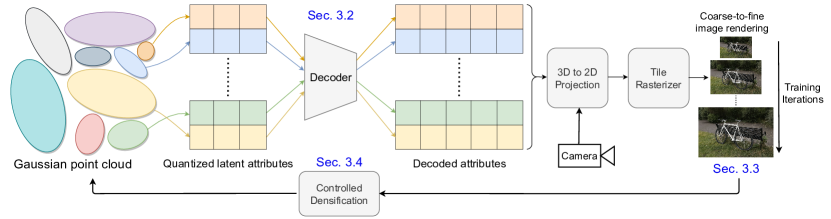
Figure 2: Approach: 1) We quantize the attributes of the latents to reduce the storage memory of the Gaussians (Sec. 4.1), 2) progressively train using a coarse-to-fine rendering resolution schedule to obtain higher quality reconstructions (Sec. 4.2) and 3) control the densification process to obtain fewer Gaussians and faster training/rendering speeds (Sec. 4.3).

Compression for neural fields. Several neural field compression approaches [36, 41, 38] propose a meta learning approach that learns a network on auxiliary datasets which can provide a good initialization for the downstream network. While our method can benefit from meta-learning as well, we restrict our current approach to compressing a single scene for brevity. VQAD [40] propose a vector quantization for a hierarchical feature grids used in NGLOD[39]. Their method is able to achieve higher compression as compared to other feature-grid methods such as Instant NGP [29] however its training can be memory intensive and it struggles to achieve the same quality of reconstructions as compared to some other NeRF variants such as MipNeRF. [25] propose a similar compression approach using voxel pruning and codebook quantization. Scalar quantization approaches such as SHACIRA [16, 4] reparameterize the network weights with integers and apply further entropy regularization to compress the scene even further. While these approaches require lower training memory as compared to  [39], they are sensitive to hyperparameters and the reconstruction efficacy of these approaches remain lower as compared to MipNeRF360 or Gaussian Splatting.

In this work, we show for the first time, that it is possible to compress 3D Gaussian point cloud representations which can retain high reconstruction quality with much smaller memory and higher FPS for inference.

3 Background

3D Gaussian splatting consists of a Gaussian point cloud representation in 3D space. Each Gaussian consists of various attributes such as the position (for mean), scaling and rotation coefficients (for covariance), opacity and color. These Gaussians represent a 3D scene and are used for rendering images from certain viewpoints by anisotropic volumetric “splatting” [45, 46] of 3D Gaussians onto a 2D plane. This is done by projecting the 3D points to 2D and then using a differentiable tile-based rasterizer for blending together different Gaussians.

3D Gaussians with a mean 3D position vector $\boldsymbol{x}$ and covariance matrix $\Sigma$ can be defined as

$$G(\boldsymbol{x})=e^{-\frac{1}{2}\boldsymbol{x}^{T}\Sigma^{-1}\boldsymbol{x}}$$ (1)

The 3D covariance matrix is in turn defined using a scale matrix S (represented using a 3D scale vector $s$) and rotation matrix R (represented using a 4D rotation vector $r$) as

$$\Sigma=RSS^{T}R^{T}$$ (2)

For a camera viewpoint with a projective transform P (world-to-camera matrix) and J as the Jacobian of the affine approximation of the projective transform, the corresponding covariance matrix projection [20] to 2D is written as:

$$\Sigma^{\prime}=JP\Sigma P^{T}J^{T}$$ (3)

The color of a pixel C is then computed using $\mathcal{N}$ Gaussian points overlapping the pixel. The points are sorted based on their opacity values $\alpha$ and blended as:

$$C=\sum_{i\in\mathcal{N}}\boldsymbol{c}_{i}\alpha_{i}\prod_{j=1}^{i-1}(1-\alpha_{j})$$ (4)

where $\alpha_{i}$ is computed by computing the 2D Gaussian multiplied with a scalar opacity value. The color $c_{i}$ of each Gaussian is then computed using spherical harmonic coefficients [35].

The Gaussians are initialized using the sparse point clouds created by SfM [43]. Further optimization of the attributes are then done using Stochastic Gradient Descent as the rendering process is fully differentiable. For each view sampled from the training dataset, the corresponding image is projected and rasterized with the forward process explained above. The reconstruction loss is then computed by combining $\mathcal{L}_{1}$ with SSIM loss as

$$\mathcal{L}=(1-\lambda)\mathcal{L}_{1}+\lambda\mathcal{L}_{\text{SSIM}}$$ (5)

with $\lambda$ set to 0.2.

Another key step in the optimization of the Gaussians is controlling the number of Gaussians. After a warmup-phase, Gaussians with a low opacity value $\alpha$ below a threshold are removed every 100 iterations. Additionally, large Gaussians (bigger than the corresponding geometry) are split while small Gaussians are cloned in order to better fit the underlying geometric shape. Only Gaussians with positional gradients above a threshold $\tau_{thresh}$ after every 100 iterations are split or cloned.

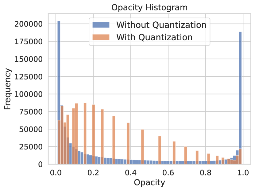
Figure 3: Histogram of opacity coefficients with and without quantization. Most coefficients result in values of 0 or 1 without quantization while quantization spreads the opacity values and allows for better blending.

4 Method

4.1 Attribute quantization

Each Gaussian point consists of a position vector $\boldsymbol{p}\in\mathbb{R}^{3}$, scaling coefficient $\boldsymbol{s}\in\mathbb{R}^{3}$, rotation quarternion vector $\boldsymbol{r}\in\mathbb{R}^{4}$, opacity scalar $o\in\mathbb{R}$ and spherical harmonics coefficients $\boldsymbol{c}\in\mathbb{R}^{d}$, with $d=3*f^{2}$, where $f$ corresponds to the harmonics degree. Thus, for a degree of 4 (as is used in [21]), the color coefficients make up more than $80\%$ of the dimensions of the full attribute vector. 3D-GS typically requires millions of Gaussians for representing the scene with high quality. However, a set of 1 million Gaussians consume around 236 MB of disk space when storing the full attribute vector with a 32-bit floating point. Thus, to reduce the memory required for storing each attribute vector, we propose to use a set of quantized representations. A visualization of the various components of our approach is provided in Fig. 2.

For any given attribute, we maintain a quantized latent vector $\boldsymbol{q}\in\mathbb{Z}^{l}$ with dimension $l$, consisting of integer values. We then use an MLP decoder $D:\mathbb{Z}^{l}{\rightarrow}\mathbb{R}^{k}$ to decode the latents and obtain the attributes. As quantized vectors are not differentiable, we maintain continuous approximations $\widehat{\boldsymbol{q}}$ during training and use the Straight-Through Estimator (STE) which rounds off $\widehat{\boldsymbol{q}}$ to the nearest integer and directly passes the gradient during backpropagation. We get

$$\boldsymbol{a}=D(STE(\widehat{\boldsymbol{q}}))$$ (6)

The latents are thus trained end-to-end similar to the standard procedure of 3D-GS. Post training, we round $\widehat{\boldsymbol{q}}$ to the nearest integer and use entropy coding for efficiently storing the latents along with the decoder $D$. While each vector in the attribute set $\mathbb{A}=\{\boldsymbol{p},\boldsymbol{s},\boldsymbol{r},\boldsymbol{c},o\}$ can be quantized, we do not encode the base band color SH coefficient, the scaling coefficients and the position vector as they are sensitive to initialization and result in large performance drops when quantized.

While the color and rotation attributes are quantized to reduce the memory footprint, we additionally quantize the opacity coefficients as well as they improve the optimization process resulting in lesser artifacts in the rendered views. In Fig. 3, we visualize the histogram of opacity coefficients of all Gaussian points, with and without quantization. We see that most points converge to 0 or 1 without quantization while quantizing produces a better spread of opacity values. A large number of points with opacity value 1 leads to the rasterization process for each pixel saturating with very few Gaussians. In contrast, the quantized distribution allows for a better blend of multiple Gaussians for each pixel. In Sec. 5.3, we show how opacity quantization has the added benefit of removing artifacts normally present in 3D-GS.

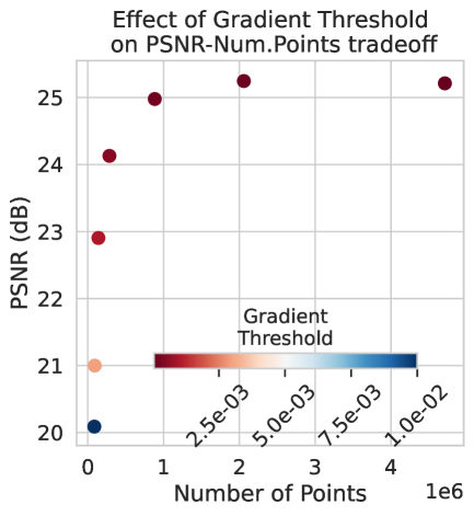
(a)	(b)

Figure 4: Effect of densification interval and gradient threshold. Higher interval or lower threshold leads to fewer Gaussians with little PSNR drop until the knee point in the curve (noise range).

Table 1: Comparison of our approach with prior work in view synthesis on three datasets. * corresponds to our runs on the existing codebase for fair evaluation. We perform competitively in terms of reconstruction metrics while outperforming in terms of efficiency metrics.

Dataset ($\rightarrow$)	Mip-NeRF360						Tanks&Temples						Deep Blending
Method	PSNR $\uparrow$	SSIM $\uparrow$	LPIPS $\downarrow$	Storage Mem $\downarrow$	FPS $\uparrow$	Train Time $\downarrow$	PSNR $\uparrow$	SSIM $\uparrow$	LPIPS $\downarrow$	Storage Mem $\downarrow$	FPS $\uparrow$	Train Time $\downarrow$	PSNR $\uparrow$	SSIM $\uparrow$	LPIPS $\downarrow$	Storage Mem $\downarrow$	FPS $\uparrow$	Train Time $\downarrow$
Plenoxels	23.08	0.63	0.46	2.1GB	7	25m49s	21.08	0.72	0.38	2.3GB	13	25m5s	23.06	0.80	0.51	2.7GB	11	27m49s
INGP	25.59	0.70	0.33	48MB	9	7m30s	21.92	0.75	0.31	48MB	14	6m59s	24.96	0.82	0.39	48MB	3	8m
M-NeRF360	27.69	0.79	0.24	9MB	0.06	48h	22.22	0.76	0.26	9MB	0.14	48h	29.40	0.90	0.25	8.6MB	0.09	48h
3D-GS	27.21	0.82	0.21	734MB	134	41m33s	23.61	0.84	0.18	411MB	154	26m54s	29.41	0.90	0.24	676MB	137	36m2s
3D-GS*	27.45	0.81	0.22	746MB	113	23m14s	23.61	0.85	0.18	427MB	161	11m9s	29.48	0.90	0.25	656MB	125	18m40s
Ours-Small	26.94	0.80	0.25	47MB	166	17m3s	23.26	0.83	0.21	26MB	283	8m54s	29.84	0.91	0.25	43MB	195	14m31s
Ours-21K	26.89	0.80	0.25	69MB	136	11m50s	23.09	0.83	0.22	34MB	245	7m13s	29.75	0.91	0.26	62MB	159	10m15s
Ours-30K	27.15	0.81	0.24	68MB	137	19m59s	23.41	0.84	0.20	34MB	244	9m51s	29.91	0.91	0.25	62MB	160	17m29s

4.2 Progressive training

Standard training of the Gaussians proceeds by computing the loss over the full image resolution. This results in a more complex loss landscape as the Gaussians are forced to fit to fine features of the scene early in the training. As the SfM initialization is only sparse and several attributes are initialized with rough estimates, the optimization can be suboptimal and result in floating artifacts from Gaussians which cannot be removed during the optimization. We thus propose a coarse-to-fine training strategy by initially rendering at a small scene resolution and gradually increasing the size of the rendered image views over a period of the training iterations until reaching the full resolution. By starting with small images, the Gaussian points easily converge to a good loss minima. This produces better initializations for the creation of further Gaussians through the densification process of cloning and splitting. As the render resolution increases, more Gaussians can be fit to better reconstruct the finer features of the scene. Such a progressive training procedure also helps remove artifacts typically obtained from the rasterization of ill-optimized Gaussians as we show in Sec. 5.3. This serves as a soft regularization scheme for the creation and deletion of Gaussians. Another added benefit of progressive training is that fewer Gaussians are required to represent coarser scenes, thereby leading to faster rendering and backpropagation during training. This directly leads to lower training times while still improving the reconstruction quality of the scene upon convergence.

4.3 Controlled Densification

The densification process of cloning and splitting occurs every 100 iterations. This, however, leads to an explosion in the number of Gaussians as a large number of Gaussians exceed the gradient threshold and are either cloned or split. While this can allow for representing finer details in the scene, a significant fraction of the Gaussians are redundant and lead to large training, rendering times as well as memory usage. We visualize this in Fig. 4 by training on a 3D scene. Results are averaged over 3 runs. We vary the gradient threshold for densification in (a) or the interval for densification in (b). A larger threshold leads to fewer Gaussians being densified (x-axis) but still results in little to no drops in reconstruction performance in terms of PSNR (y-axis). Alternately, increasing the densification interval results in Gaussians being densified less frequently and also has a similar effect of faster rendering speed in terms of FPS (x-axis). There exists a distinct trade-off between reconstruction quality and efficiency, in terms of size or FPS. However, substantial efficiency improvements can be achieved until reaching the inflection point of the curve, with minimal compromise in performance. We identify the optimal point in the gradient threshold and the densification interval and use it for all our experiments.

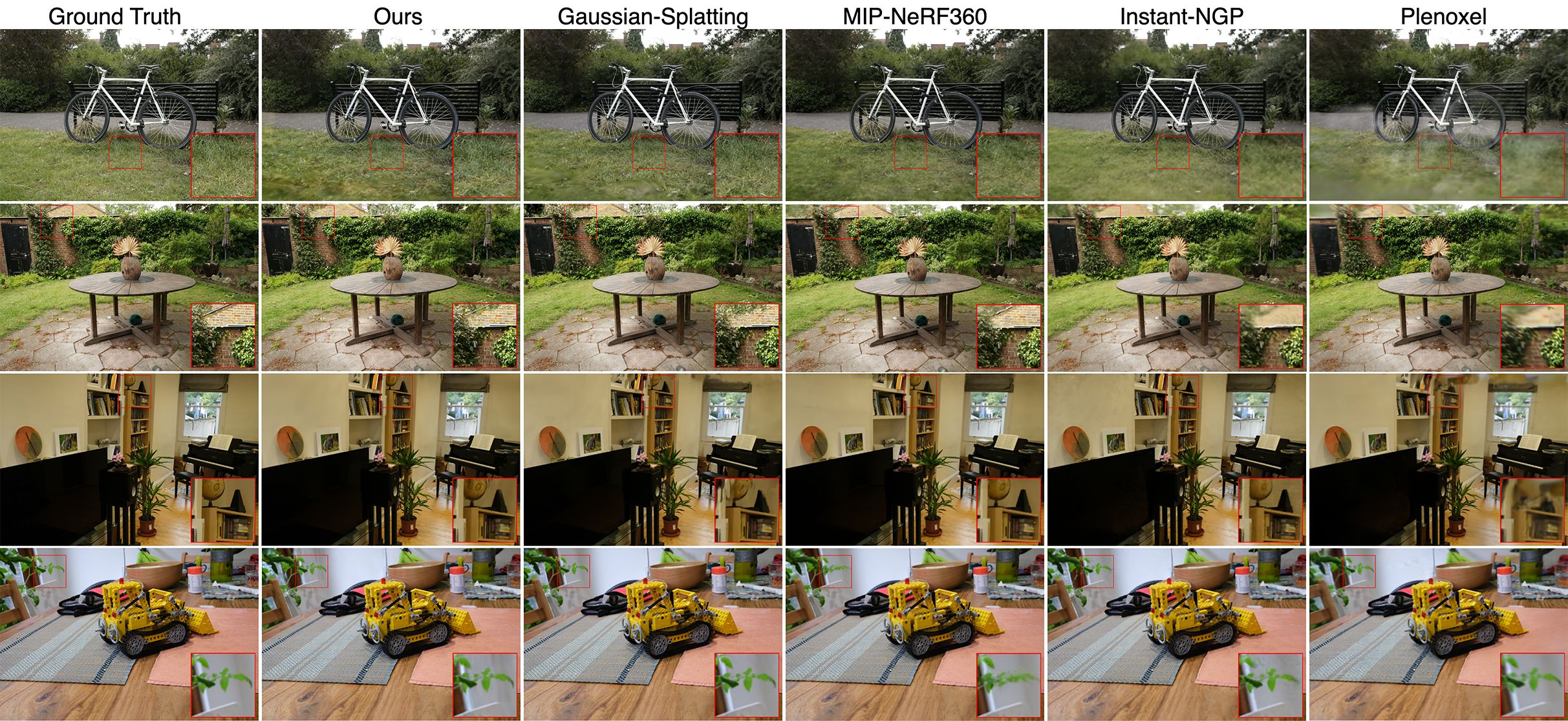
Figure 5: Qualitative comparison. We obtain on par or better reconstructions with the SOTA 3D-GS and MiP-NeRF360 while INGP, Plenoxels struggle to reconstruct fine detail. We avoid the floaters or blurry artifacts at scene edges exhibited by 3D-GS and MiP-NeRF360.

5 Experiments

5.1 Implementation and evaluation

We implemented our method by building on [21] which uses a PyTorch framework [31] with a CUDA backend for the rasterization operation.

A full list of the hyperparameters (learning rates, architecture, initialization of the latents) is provided in the supplementary material. For the progressive scaling, we start with a scale factor of 0.3 while increasing to 1.0 in a cosine schedule. We provide sensitivity analysis of this scale factor in Sec. 5.3. We perform the scaling schedule for 70% of the total iterations after which training continues at the full resolution. We fix the opacity reset interval to be every 2500 iterations and the densification frequency to be 250 iterations. We optimize for 30000 iterations but can be controlled based on the time and memory budget for training. We fix the SH degree to be 3 for the color attribute as higher values result in little performance gain for a large increase in memory cost, even with quantization. We use this configuration of hyperparameters for all of our experiments unless mentioned otherwise.

We provide results on 9 scenes from the Mip-Nerf360 dataset [3], and 2 scenes each from Tanks&Temples [22], Deep Blending [19] for a total of 13 scenes. These datasets correspond to real-world high resolution scenes which can be unbounded and provide a challenging scenario with parts of the scene scarcely seen during training. We follow the methodology of [21, 3] with every 8th view used for evaluation and the rest for training. We evaluate the quality of reconstructions primarily with PSNR, and also with the SSIM and LPIPS metrics. We calculate memory of all quantized and non-quantized parameters of the Gaussians for the storage size. The rendering and training memory measures the peak GPU RAM for the full training/rendering phase. We measure the frame rate or Frames Per Second (FPS) based on the time taken to render from all cameras in the scene dataset. Before measuring FPS, we decode all latent attributes using our decoder which is a one-time amortized cost of loading the parameters. For a fair benchmark, the quantitative results comparison of other works in Tab. 1 are provided by using the numbers reported in [21], unless mentioned otherwise. The qualitative results are from our own runs of the respective methods.

5.2 Benchmark comparison

For NeRFs, we compare against the SOTA method MipNerf360 [3] and two recent fast NeRF approaches of INGP [29], and Plenoxels [13]. For our primary baseline, 3D-GS, we provide numbers as reported in [21] and also from our own runs. We show results of our approach for 3 variants: a) A smaller configuration corresponding to higher densification interval b) training for 21K iterations which is the end of the progressive training schedule, and c) training for 30K iterations which is until convergence. We summarize the results on all 3 datasets in Table 1.

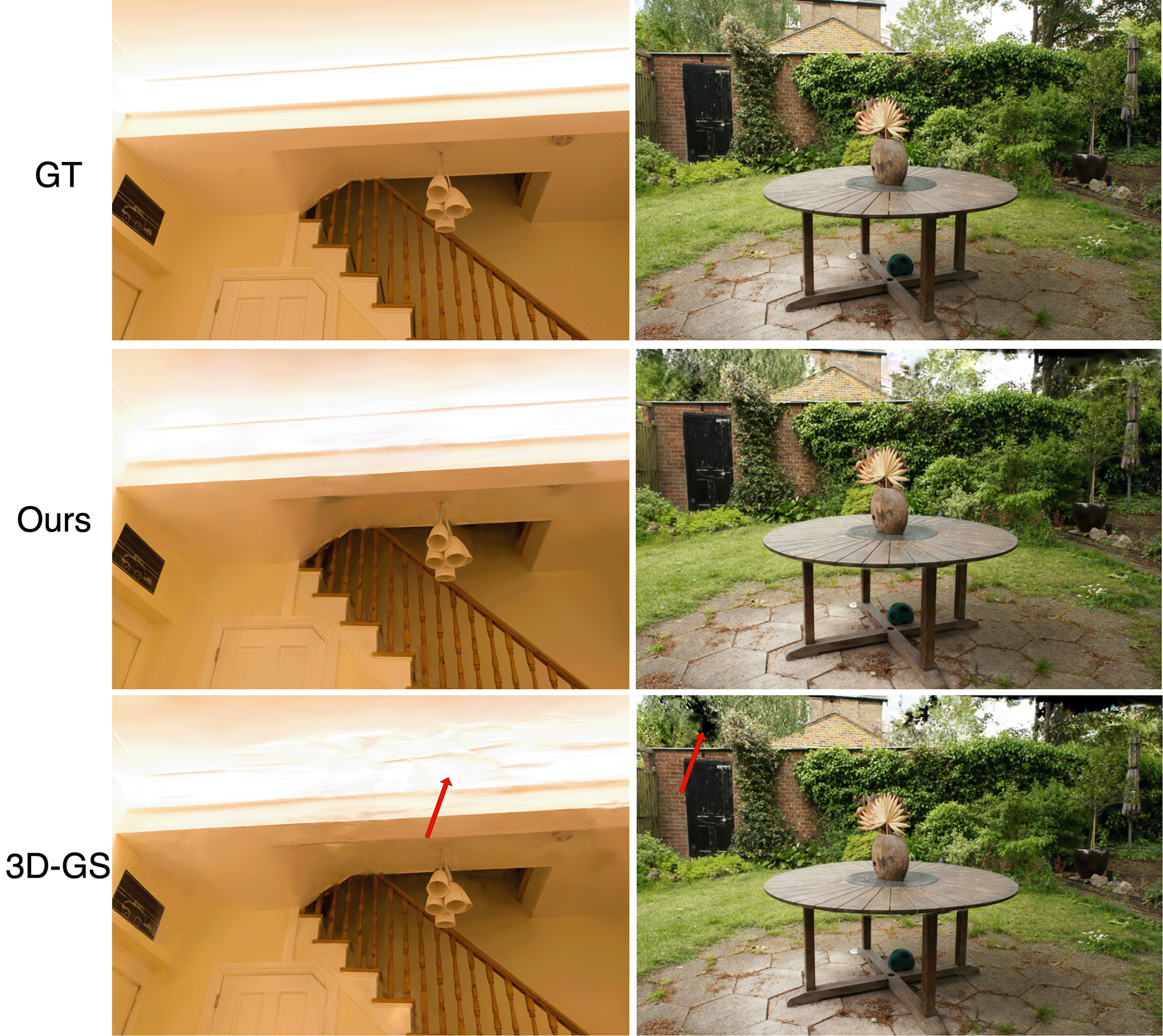
Figure 6: 3D-GS produces artifacts at various scene locations (red arrow) while our rendering aligns more with the ground truth.

Table 2: Ablation of various components of our approach. Attribute quantization significantly reduces the storage memory for a marginal PSNR cost. Progressive training improves the PSNR due to better optimization while less frequent densification signficantly speeds up training and rendering while also reducing storage size at the same or higher PSNR.

Method

Train (Tanks & Temples)

Dr Johnson (Deep Blending)

Bicycle (Mip-NERF360)

PSNR

Storage Mem

Num. Gaussians

FPS

PSNR

Storage Mem

Num. Gaussians

FPS

PSNR

Storage Mem

Num. Gaussians

FPS

Vanilla

21.88dB

259MB

1.10M

181

29.08dB

767MB

3.25M

104

25.10dB

1334MB

5.67M

60

+ Quantization

21.59dB

49MB

1.09M

162

28.84dB

163MB

3.39M

84

24.80dB

206MB

4.46M

65

+ Progressive

21.74dB

40MB

0.88M

194

29.22dB

146MB

3.32M

75

25.10dB

204MB

4.48M

70

+ Densification

21.86dB

25MB

0.55M

244

29.54dB

80MB

1.82M

109

24.94

113MB

2.47M

98

We outperform the voxel-grid based method of Plenoxels on all datasets and metrics. Compared to INGP [29], another fast Nerf-based method, our approach at 21K iterations, obtains better quality reconstructions at comparable training times on Tanks&Temples, Deep Blending but higher training times for Mip-NeRF360. We bridge the gap between NeRF-based methods and Gaussian Splatting in terms of storage memory, by obtaining comparable sizes to INGP (Ours-Small configuration) while still obtaining better reconstruction metrics. We also obtain much higher rendering speeds (${>}15{\times}$) compared to INGP on all datasets paving the way for compact 3D representations with high quality reconstructions and real-time rendering. Against the Mip-NeRF360 approach, we perform competitively in terms of PSNR with a 0.5 dB drop on their dataset and 1.2dB,0.5dB gain on Tanks&Temples, Deep Blending respectively. While their model is compact in terms of number of parameters they are extremely slow to train (${\sim}48$h) and render (${<}1$FPS). Finally, our reconstructions are on par with 3D-GS achieving minimal performance drops of 0.3dB, 0.2dB PSNR on the Mip-NeRF360, Tanks&Temples datasets respectively while gaining 0.5dB on Deep Blending. We reduce the storage size by more than an order of magnitude making the representation suitable for devices with limited memory budgets. Additionally, we accelerate training and rendering compared to 3D-GS obtaining higher FPS and lower train times on all scenes. We additionally see that our approach reaches close to convergence with good visual quality at 21K iterations itself (marking the end of the progressive scaling period). Note that a fair amount of time is spent on training after 21K iterations due to the full scale render resolution.

We show qualitative results of our approach on and other baselines on unseen test views from indoor and outdoor scenes in Fig. 5. Mip-NeRF360 exhibits blurry artifacts such as the grass in the Bicycle scene (top) or the house in the Garden scene (2nd from top) or even incorrect artifacts as seen in the edges of the leaf in Kitchen (bottom). We obtain reconstructions with quality on-par with 3D-GS or even better reconstructions at edges of the scene such as the globe in Room (3rd from top). Notably, 3D-GS tends to exhibit numerous floaters at the edges, especially in areas not frequently observed during training. We provide additional visualizations of this in Fig. 6, showcasing notably smoother reconstructions at scene edges, such as the Room’s ceiling (left), and a reduction in dark artifacts, as observed in the Garden scene (right). This points to a more refined optimization of the point cloud using our approach. We ablate the different components of our approach and analyze the effects of each component in Sec. 5.3 below.

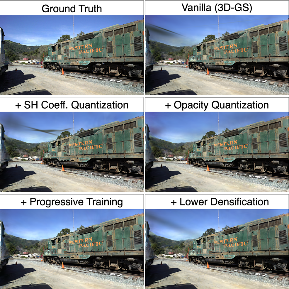
Figure 7: Opacity quantization and progressive retraining removes floaters. Increasing the densification interval to reduces the number of Gaussians but reintroduces artifacts to a limited extent.

5.3 Ablations

For a deeper understanding of our approach, we provide qualitative and quantitative results for three scenes, gradually incorporating each component step by step. Results are summarized in Table 2 and Fig. 7. ”Vanilla” effectively corresponds to the baseline 3D-GS. First, we quantize the color, rotation and opacity attributes for each Gaussian. We get a significant reduction in storage memory with a small drop in PSNR or reconstruction quality. Note that the bulk of the memory post quantization is from the non quantized attributes of scale, position, base color. The quantized attributes are compressed from 211 MB, 633 MB, 1107 MB to 6 MB, 27 MB, 28 MB for the 3 scenes respectively achieving $20{-}30{\times}$ memory reduction. We visualize the effect of color and rotation quantization for a single unseen view from the ”Train” scene in Fig. 7. Notice the floaters/rendering artifacts at the top left of the scene as it has little overlap with training views for the vanilla configuration. Quantizing color and rotation does not directly remove these artifacts but opacity quantization significantly improves the visual quality of the rendering.

We then include progressive scaling increasing the rendering resolution in a cosine schedule. We achieve gains in PSNR with fewer floating artifacts due to a more stable optimization while significantly reducing training time as we show in Tab. 3. Progressive scaling also provides a better optimization of the loss landscape removing any remaining foggy artifacts as seen in Fig. 7. Finally, increasing the densification interval significantly decreases the number of Gaussians resulting in lower storage memory, training time, and higher FPS without sacrificing heavily on reconstruction quality in terms of PSNR. This reintroduces artifacts in the specific view depicted in Fig. 7, although to a considerably lesser extent compared to the standard 3D-GS.

To further analyze the strength of progressive training, we vary the resize scale and visualize the PSNR-model size tradeoff and the convergence speed as well in Fig. 8(a),(b). We run experiments on the Truck scene and average over 3 random seeds with error intervals reported. From (a), we see that decreasing the scale upto 0.3 has no effect on PSNR but reduces the number of Gaussians needed to represent that scene. Beyond this value, dropoffs in PSNR is observed for lower storage memory. In (b), we analyze the convergence speed in terms of the iteration time over the course of training for various scaling values. As expected, we consistently obtain lower iteration time for lower scale values even with no loss in PSNR as seen in (a).

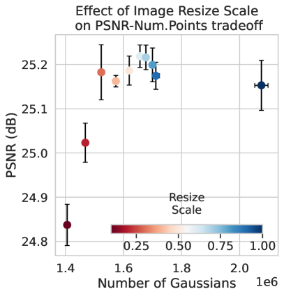
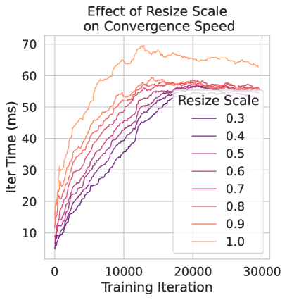
(a)	(b)

Figure 8: Effect of progressive resize scale. (a) Decreasing the scale value leads to reductions in number of Gaussians with no cost to PSNR. (b) This also improves the training speed requiring lesser time per iteration.

5.4 Progressive scaling variants

As explained previously, progressive scaling of the scene while training provides stable optimizations. We now analyze the effect of applying different types of filters to the image as part of the coarse-to-fine training procedure. Results are summarized in Table 3. We try different types of strategies such as a) the mean filter which corresponds to downsampling and re-upsampling the image with bilinear interpolation b) a gaussian filter c) the standard downsampling procedure as used for our experiments and d) with no type of progressive training. For downsampling and mean filtering, we start with a scale of 0.3 and end at 1.0 which corresponds to resizing the image to 30% of its dimensions and scaling upto its original size gradually for a period of 70% of the iterations. For Gaussian filtering, we progressively decrease the filter size from the initial value specified in the table down to $1\times 1$, which essentially equates to no filtering. Compared to the no filter case, all other types of filters result in fewer Gaussians leading to lower memory, training time and higher FPS. Both Gaussian and Mean filters provide large gains in terms of efficiency metrics with little to no drops in PSNR. The Gaussian filter naturally provides a coarse-to-fine schedule for training Gaussian points. Nonetheless, the training still proceeds at full resolution and the largest gains in terms of training time is produced with downsampling. The $5\times 5$ Gaussian filter produces similar results as downsampling albeit with higher training times while we observe a larger Gaussian filter $15\times 15$ leads to much higher efficiency at the cost of PSNR.

Table 3: Various types of progressive scaling. Downsampling reduces training time the most while high Gaussian filter sizes improves size and FPS at the cost of reconstruction quality.

Filter Type	PSNR	Storage Mem	Num. Gaussians	FPS	Training Time
None	23.34dB	43MB	0.95M	211	13m27s
Mean	23.31dB	27MB	0.61M	280	11m41s
Gaussian $(5{\times}5)$	23.41dB	34MB	0.74M	248	12m8s
Gaussian $(7{\times}7)$	23.36dB	28MB	0.61M	276	11m32s
Gaussian $(15{\times}15)$	23.17dB	21MB	0.46M	321	10m51s
Downsample	23.41dB	34MB	0.75M	244	9m49s

Table 4: We require much lesser training and rendering memory consumption by ours and 3D-GS across all scenes consistently.

Method	Bicycle		Truck		Playroom
	Train	Render	Train	Render	Train	Render
3D-GS	17.4G	9.5G	8.5G	4.8G	9.6G	6.0G
Ours	10G	7.4G	5.3G	3.6G	7.1G	5.3G

5.5 Training and Rendering Memory

In this section, we show the memory consumption of our approach and 3D-GS on the 3 datasets in Table 4. We measure peak GPU memory used during the training or rendering phase by our approach and 3D-GS. We see that we require much lesser memory during training even with latents and decoders. Since our quantization decodes the latents to floating point values before a forward or backward pass, no gains are obtained in terms of runtime memory consumption for each Gaussian. However, with progressive training and higher densification interval, we obtain significantly lower number of Gaussians leading to lower runtime memory during training/rendering. For the Bicycle scene especially, compared to the 17G required by 3D-G, we consume only 10G GPU RAM during training making it practical for many consumer GPUs with 12G RAM.

6 Conclusion

In this work, we proposed a simple yet powerful approach for 3D reconstruction and novel view synthesis. We build upon the seminal work on 3D Gaussian Splatting [21], and propose major improvements that not only reduces the storage requirements for each scene by 10-20$\times$, but also achieves it with lower training cost, faster inference time, and on par reconstruction quality. We achieve this by 3 major improvements over the prior work - attribute quantization, progressive training, and controlled densification. Our extensive quantitative and qualitative analyses shows the efficacy of our approach in 3D representation.

Acknowledgements: This project was partially supported by IARPA WRIVA program (Contract No. 140D0423C0076). We also thank Jon Barron for providing additional scenes from the Mip-NeRF360 dataset for our experiments.

Supplementary Material

7 Hyperparameters

We compress the color, rotation and opacity attributes of each Gaussian as explained in the main paper. Each attribute consists of several hyperparameters; mainly latent dimension, decoder parameter learning rate, latent learning rate, decoder initialization. The decoder parameters are initialized using a normal distribution with a standard deviation. As the uncompressed attributes $\boldsymbol{a}$ are initialized using SfM for 3D-GS [21], we obtain the latent initialization (with continuous approximations $\widehat{\boldsymbol{q}}$) simply by inverting the decoder $D$.

$$\widehat{\boldsymbol{q}}=D^{-1}(\boldsymbol{a})$$ (7)

For a decoder which is only a linear layer, a least square approximation provides the latent values. The learning rate of the latents is obtained by scaling the original attribute learning rate with a scale factor and divided by the norm of the decoder (for a linear layer). This improves training stability and convergence when decoder norm is either too high or too low. Values used for all the compressible attributes are provided in Tab. 5. We use these values for all of our experiments and find it to be stable across various datasets. All other hyperaparameter values are used as is the default in [21].

Table 5: Latent hyperparameter values.

Attribute	Latent Dimension	Decoder LR	Decoder Std.	Latent LR Scale
Color	16	0.005	0.0005	0.1
Rotation	8	0.01	0.01	0.1
Opacity	1	0.3	0.5	0.1

8 Per scene metrics

We provide metrics for each scene across the 3 datasets of Mip-NeRF360, Tanks&Temples, and Deep Blending in Table 7, Table 8, Table 9 respectively.

9 Synthetic scenes

In addition to real scenes shown in Sec. 8, we perform evaluation on 10 Bricks scenes from the RTMV dataset [42]. Results are summarized in Table 6 for scenes at $400{\times}400$ resolution as is typically used. Numbers apart from 3D-GS and ours are copied from the papers. Both 3D-GS and our approach achieve similar or better performance than many NeRF-based variants while being significantly faster in terms of training convergence speed. In addition, we reduce the average model size from ${\approx}63MB$ of 3D-GS to ${\approx}5MB$ in range within most other methods. We also obtain faster training times and improve rendering speed from 365 for 3D-GS to 789 for ours. This is more than an order of magnitude over many other approaches. We continue to obtain high FPS (345) even for the full resolution $1600{\times}1600$ providing sufficient capacity of real-time rendering for even higher resolutions.

Table 6: RTMV results

Method	PSNR	SSIM	LPIPS	Storage Mem	Train Time
NeRF [28]	28.28	0.9398	0.0410	2.5MB	-
mip-NERF [2]	31.61	0.9582	0.0214	1.2MB	-
NGLOD [39]	32.72	0.9700	0.0379	$\approx$20MB	-
VQAD [40]	31.45	0.9638	0.0468	0.55MB	$\approx$30m
Instant-NGP [29]	31.88	0.9690	0.0381	48.9MB	$\approx$12m
3D-GS [21]	32.35	0.9792	0.0213	63.3MB	3m33s
Ours	32.21	0.9772	0.0240	4.6MB	2m45s

Table 7: MiP-NeRF360 per scene results

Scene	Method	PSNR	SSIM	LPIPS	Storage Mem	FPS	Train Time	Num. Gaussians
Bicycle	Ours	24.91	0.74	0.26	112MB	97	22m 44s	2.46M
	3D-GS	25.13	0.75	0.24	1342MB	60	28m 36s	5.69M
Bonsai	Ours	31.44	0.94	0.19	36MB	184	16m 42s	0.82M
	3D-GS	31.94	0.95	0.18	294MB	188	18m 22s	1.25M
Counter	Ours	28.47	0.91	0.20	32MB	147	18m 56s	0.71M
	3D-GS	29.09	0.92	0.19	275MB	143	21m 23s	1.17M
Flowers	Ours	21.00	0.57	0.38	69MB	161	17m 25s	1.55M
	3D-GS	21.32	0.59	0.36	821MB	107	22m 0s	3.48M
Garden	Ours	26.88	0.84	0.16	85MB	123	21m 23s	1.92M
	3D-GS	27.32	0.86	0.12	1336MB	67	28m 52s	5.66M
Kitchen	Ours	30.70	0.93	0.13	57MB	107	23m 33s	1.28M
	3D-GS	31.43	0.93	0.12	417MB	112	25m 29s	1.77M
Room	Ours	31.84	0.93	0.20	36MB	143	19m 17s	0.80M
	3D-GS	31.61	0.93	0.20	357MB	137	21m 23s	1.51M
Stump	Ours	26.59	0.77	0.26	112MB	141	19m 37s	2.44M
	3D-GS	26.64	0.77	0.24	1059MB	99	22m 9s	4.49M
Treehill	Ours	22.57	0.64	0.36	81MB	132	20m 3s	1.79M
	3D-GS	22.56	0.64	0.35	829MB	104	21m 38s	3.51M
Average	Ours	27.15	0.81	0.24	69MB	137	19m 58s	1.53M
	3D-GS	27.45	0.81	0.22	748MB	113	23m 19s	3.17M

Table 8: Tanks&Temples per scene results

Scene	Method	PSNR	SSIM	LPIPS	Storage Mem	FPS	Train Time	Num. Gaussians
Truck	Ours	25.09	0.87	0.17	43MB	245	9m 55s	0.96M
	3D-GS	25.37	0.88	0.15	593MB	141	12m 6s	2.51M
Train	Ours	21.74	0.80	0.23	25MB	244	9m 42s	0.55M
	3D-GS	21.85	0.81	0.21	261MB	181	10m 21s	1.10M
Average	Ours	23.41	0.84	0.20	34MB	244	9m 49s	0.76M
	3D-GS	23.61	0.85	0.18	427MB	161	11m 13s	1.81M

Table 9: Deep Blending per scene results

Scene	Method	PSNR	SSIM	LPIPS	Storage Mem	FPS	Train Time	Num. Gaussians
Playroom	Ours	30.32	0.91	0.25	44MB	212	14m 17s	0.98M
	3D-GS	29.93	0.90	0.25	543MB	147	16m 42s	2.30M
Dr Johnson	Ours	29.50	0.91	0.24	81MB	109	20m 32s	1.82M
	3D-GS	29.03	0.90	0.25	768MB	103	21m 2s	3.26M
Average	Ours	29.91	0.91	0.25	62MB	160	17m 24s	1.40M
	3D-GS	29.48	0.90	0.25	656MB	125	18m 52s	2.78M

References

- Banner et al. [2018] Ron Banner, Yury Nahshan, Elad Hoffer, and Daniel Soudry. Post-training 4-bit quantization of convolution networks for rapid-deployment. arXiv preprint arXiv:1810.05723, 2018.
- Barron et al. [2021] Jonathan T Barron, Ben Mildenhall, Matthew Tancik, Peter Hedman, Ricardo Martin-Brualla, and Pratul P Srinivasan. Mip-nerf: A multiscale representation for anti-aliasing neural radiance fields. In Proceedings of the IEEE/CVF International Conference on Computer Vision, pages 5855–5864, 2021.
- Barron et al. [2022] Jonathan T Barron, Ben Mildenhall, Dor Verbin, Pratul P Srinivasan, and Peter Hedman. Mip-nerf 360: Unbounded anti-aliased neural radiance fields. In Proceedings of the IEEE/CVF Conference on Computer Vision and Pattern Recognition, pages 5470–5479, 2022.
- Bird et al. [2021] Thomas Bird, Johannes Ballé, Saurabh Singh, and Philip A Chou. 3d scene compression through entropy penalized neural representation functions. In 2021 Picture Coding Symposium (PCS), pages 1–5. IEEE, 2021.
- Chen et al. [2021] Hao Chen, Bo He, Hanyu Wang, Yixuan Ren, Ser Nam Lim, and Abhinav Shrivastava. Nerv: Neural representations for videos. Advances in Neural Information Processing Systems, 34:21557–21568, 2021.
- Chen et al. [2015] Wenlin Chen, James Wilson, Stephen Tyree, Kilian Weinberger, and Yixin Chen. Compressing neural networks with the hashing trick. In International conference on machine learning, pages 2285–2294. PMLR, 2015.
- Chen et al. [2016] Wenlin Chen, James Wilson, Stephen Tyree, Kilian Q Weinberger, and Yixin Chen. Compressing convolutional neural networks in the frequency domain. In Proceedings of the 22nd ACM SIGKDD International Conference on Knowledge Discovery and Data Mining, pages 1475–1484, 2016.
- Courbariaux et al. [2015] Matthieu Courbariaux, Yoshua Bengio, and Jean-Pierre David. Binaryconnect: Training deep neural networks with binary weights during propagations. In Advances in neural information processing systems, pages 3123–3131, 2015.
- Dettmers et al. [2022] Tim Dettmers, Mike Lewis, Younes Belkada, and Luke Zettlemoyer. Llm. int8 (): 8-bit matrix multiplication for transformers at scale. arXiv preprint arXiv:2208.07339, 2022.
- Dupont et al. [2021] Emilien Dupont, Adam Goliński, Milad Alizadeh, Yee Whye Teh, and Arnaud Doucet. Coin: Compression with implicit neural representations. arXiv preprint arXiv:2103.03123, 2021.
- Frankle and Carbin [2018] Jonathan Frankle and Michael Carbin. The lottery ticket hypothesis: Finding sparse, trainable neural networks. arXiv preprint arXiv:1803.03635, 2018.
- Frankle et al. [2020] Jonathan Frankle, Gintare Karolina Dziugaite, Daniel M Roy, and Michael Carbin. Pruning neural networks at initialization: Why are we missing the mark? arXiv preprint arXiv:2009.08576, 2020.
- Fridovich-Keil et al. [2022] Sara Fridovich-Keil, Alex Yu, Matthew Tancik, Qinhong Chen, Benjamin Recht, and Angjoo Kanazawa. Plenoxels: Radiance fields without neural networks. In Proceedings of the IEEE/CVF Conference on Computer Vision and Pattern Recognition, pages 5501–5510, 2022.
- Girish et al. [2021] Sharath Girish, Shishira R Maiya, Kamal Gupta, Hao Chen, Larry S Davis, and Abhinav Shrivastava. The lottery ticket hypothesis for object recognition. In Proceedings of the IEEE/CVF Conference on Computer Vision and Pattern Recognition, pages 762–771, 2021.
- Girish et al. [2022] Sharath Girish, Kamal Gupta, Saurabh Singh, and Abhinav Shrivastava. Lilnetx: Lightweight networks with extreme model compression and structured sparsification. arXiv preprint arXiv:2204.02965, 2022.
- Girish et al. [2023] Sharath Girish, Abhinav Shrivastava, and Kamal Gupta. Shacira: Scalable hash-grid compression for implicit neural representations. In Proceedings of the IEEE/CVF International Conference on Computer Vision, pages 17513–17524, 2023.
- Gong et al. [2014] Yunchao Gong, Liu Liu, Ming Yang, and Lubomir Bourdev. Compressing deep convolutional networks using vector quantization. arXiv preprint arXiv:1412.6115, 2014.
- Han et al. [2015] Song Han, Jeff Pool, John Tran, and William J Dally. Learning both weights and connections for efficient neural networks. arXiv preprint arXiv:1506.02626, 2015.
- Hedman et al. [2018] Peter Hedman, Julien Philip, True Price, Jan-Michael Frahm, George Drettakis, and Gabriel Brostow. Deep blending for free-viewpoint image-based rendering. ACM Transactions on Graphics (ToG), 37(6):1–15, 2018.
- Hoaglin and Welsch [1978] David C Hoaglin and Roy E Welsch. The hat matrix in regression and anova. The American Statistician, 32(1):17–22, 1978.
- Kerbl et al. [2023] Bernhard Kerbl, Georgios Kopanas, Thomas Leimkühler, and George Drettakis. 3d gaussian splatting for real-time radiance field rendering. ACM Transactions on Graphics (ToG), 42(4):1–14, 2023.
- Knapitsch et al. [2017] Arno Knapitsch, Jaesik Park, Qian-Yi Zhou, and Vladlen Koltun. Tanks and temples: Benchmarking large-scale scene reconstruction. ACM Transactions on Graphics (ToG), 36(4):1–13, 2017.
- LeCun et al. [1990] Yann LeCun, John S Denker, and Sara A Solla. Optimal brain damage. In Advances in neural information processing systems, pages 598–605, 1990.
- Li et al. [2016] Fengfu Li, Bo Zhang, and Bin Liu. Ternary weight networks. arXiv preprint arXiv:1605.04711, 2016.
- Li et al. [2023] Lingzhi Li, Zhen Shen, Zhongshu Wang, Li Shen, and Liefeng Bo. Compressing volumetric radiance fields to 1 mb. In Proceedings of the IEEE/CVF Conference on Computer Vision and Pattern Recognition, pages 4222–4231, 2023.
- Luo et al. [2022] Andrew Luo, Yilun Du, Michael Tarr, Josh Tenenbaum, Antonio Torralba, and Chuang Gan. Learning neural acoustic fields. Advances in Neural Information Processing Systems, 35:3165–3177, 2022.
- Maiya et al. [2022] Shishira R Maiya, Sharath Girish, Max Ehrlich, Hanyu Wang, Kwot Sin Lee, Patrick Poirson, Pengxiang Wu, Chen Wang, and Abhinav Shrivastava. Nirvana: Neural implicit representations of videos with adaptive networks and autoregressive patch-wise modeling. arXiv preprint arXiv:2212.14593, 2022.
- Mildenhall et al. [2020] Ben Mildenhall, Pratul P. Srinivasan, Matthew Tancik, Jonathan T. Barron, Ravi Ramamoorthi, and Ren Ng. Nerf: Representing scenes as neural radiance fields for view synthesis. In ECCV, 2020.
- Müller et al. [2022] Thomas Müller, Alex Evans, Christoph Schied, and Alexander Keller. Instant neural graphics primitives with a multiresolution hash encoding. ACM Transactions on Graphics (ToG), 41(4):1–15, 2022.
- Oktay et al. [2019] Deniz Oktay, Johannes Ballé, Saurabh Singh, and Abhinav Shrivastava. Scalable model compression by entropy penalized reparameterization. arXiv preprint arXiv:1906.06624, 2019.
- Paszke et al. [2019] Adam Paszke, Sam Gross, Francisco Massa, Adam Lerer, James Bradbury, Gregory Chanan, Trevor Killeen, Zeming Lin, Natalia Gimelshein, Luca Antiga, et al. Pytorch: An imperative style, high-performance deep learning library. Advances in neural information processing systems, 32, 2019.
- Rastegari et al. [2016] Mohammad Rastegari, Vicente Ordonez, Joseph Redmon, and Ali Farhadi. Xnor-net: Imagenet classification using binary convolutional neural networks. In European conference on computer vision, pages 525–542. Springer, 2016.
- Reed [1993] Russell Reed. Pruning algorithms-a survey. IEEE transactions on Neural Networks, 4(5):740–747, 1993.
- Savarese et al. [2020] Pedro Savarese, Hugo Silva, and Michael Maire. Winning the lottery with continuous sparsification. Advances in Neural Information Processing Systems, 33:11380–11390, 2020.
- Seeley [1966] Robert T Seeley. Spherical harmonics. The American Mathematical Monthly, 73(4P2):115–121, 1966.
- Sitzmann et al. [2020a] Vincent Sitzmann, Eric Chan, Richard Tucker, Noah Snavely, and Gordon Wetzstein. Metasdf: Meta-learning signed distance functions. Advances in Neural Information Processing Systems, 33:10136–10147, 2020a.
- Sitzmann et al. [2020b] Vincent Sitzmann, Julien Martel, Alexander Bergman, David Lindell, and Gordon Wetzstein. Implicit neural representations with periodic activation functions. Advances in neural information processing systems, 33:7462–7473, 2020b.
- Strümpler et al. [2022] Yannick Strümpler, Janis Postels, Ren Yang, Luc Van Gool, and Federico Tombari. Implicit neural representations for image compression. In Computer Vision–ECCV 2022: 17th European Conference, Tel Aviv, Israel, October 23–27, 2022, Proceedings, Part XXVI, pages 74–91. Springer, 2022.
- Takikawa et al. [2021] Towaki Takikawa, Joey Litalien, Kangxue Yin, Karsten Kreis, Charles Loop, Derek Nowrouzezahrai, Alec Jacobson, Morgan McGuire, and Sanja Fidler. Neural geometric level of detail: Real-time rendering with implicit 3d shapes. In Proceedings of the IEEE/CVF Conference on Computer Vision and Pattern Recognition, pages 11358–11367, 2021.
- Takikawa et al. [2022] Towaki Takikawa, Alex Evans, Jonathan Tremblay, Thomas Müller, Morgan McGuire, Alec Jacobson, and Sanja Fidler. Variable bitrate neural fields. In ACM SIGGRAPH 2022 Conference Proceedings, pages 1–9, 2022.
- Tancik et al. [2021] Matthew Tancik, Ben Mildenhall, Terrance Wang, Divi Schmidt, Pratul P Srinivasan, Jonathan T Barron, and Ren Ng. Learned initializations for optimizing coordinate-based neural representations. In Proceedings of the IEEE/CVF Conference on Computer Vision and Pattern Recognition, pages 2846–2855, 2021.
- Tremblay et al. [2022] Jonathan Tremblay, Moustafa Meshry, Alex Evans, Jan Kautz, Alexander Keller, Sameh Khamis, Charles Loop, Nathan Morrical, Koki Nagano, Towaki Takikawa, and Stan Birchfield. Rtmv: A ray-traced multi-view synthetic dataset for novel view synthesis. IEEE/CVF European Conference on Computer Vision Workshop (Learn3DG ECCVW), 2022, 2022.
- Ullman [1979] Shimon Ullman. The interpretation of structure from motion. Proceedings of the Royal Society of London. Series B. Biological Sciences, 203(1153):405–426, 1979.
- Zhang et al. [2018] Dongqing Zhang, Jiaolong Yang, Dongqiangzi Ye, and Gang Hua. Lq-nets: Learned quantization for highly accurate and compact deep neural networks. In Proceedings of the European conference on computer vision (ECCV), pages 365–382, 2018.
- Zwicker et al. [2001a] Matthias Zwicker, Hanspeter Pfister, Jeroen Van Baar, and Markus Gross. Ewa volume splatting. In Proceedings Visualization, 2001. VIS’01., pages 29–538. IEEE, 2001a.
- Zwicker et al. [2001b] Matthias Zwicker, Hanspeter Pfister, Jeroen Van Baar, and Markus Gross. Surface splatting. In Proceedings of the 28th annual conference on Computer graphics and interactive techniques, pages 371–378, 2001b.