SoK: Unintended Interactions among Machine Learning Defenses and Risks

Abstract

Machine learning (ML) models cannot neglect risks to security, privacy, and fairness. Several defenses have been proposed to mitigate such risks. When a defense is effective in mitigating one risk, it may correspond to increased or decreased susceptibility to other risks. Existing research lacks an effective framework to recognize and explain these unintended interactions. We present such a framework, based on the conjecture that overfitting and memorization underlie unintended interactions. We survey existing literature on unintended interactions, accommodating them within our framework. We use our framework to conjecture on two previously unexplored interactions, and empirically validate our conjectures.

1 Introduction

Potential risks to security, privacy, and fairness of machine learning (ML) models have led to various proposed defenses  [101, 118, 92, 154, 98, 40, 110, 62]. When a defense is effective against a specific risk, it may correspond to an increased or decreased susceptibility to other risks [57, 146]. For instance, adversarial training for increasing robustness also increases susceptibility to membership inference [144, 67]. We refer to these as unintended interactions between defenses and risks.

Foreseeing such unintended interactions is challenging. A unified framework enumerating different defenses and risks can help (a) researchers identify unexplored interactions and design algorithms with better trade-offs, and (b) practitioners to account for such interactions before deployment. However, prior works are limited to interactions with a specific risk (e.g., membership inference [146]) and do not systematically study the underlying causes (e.g., Gittens et al. [57]). A comprehensive framework spanning multiple defenses and risks, to systematically identify potential unintended interactions is currently absent.

We aim to fill this gap by systematically examining various unintended interactions spanning multiple defenses and risks. We conjecture that overfitting and memorization of training data are the potential causes underlying these unintended interactions. An effective defense may induce, reduce or rely on overfitting or memorization which in turn, impacts the model’s susceptibility to other risks. We identify different factors like the characteristics of the training dataset, objective function, and the model, that collectively influence a model’s propensity to overfit or memorize. These factors help us get a nuanced understanding of the susceptibility to different risks when a defense is in effect. We claim the following main contributions:

1. the first systematic framework for understanding unintended interactions, by their underlying causes and factors that influence them. (Section 3)

2. a literature survey to identify different unintended interactions, situating them within our framework, and a guideline to use our framework to conjecture unintended interactions. (Section 4)

3. identifying unexplored unintended interactions for future research, using our guideline to conjecture two such interactions, and empirically validating them. (Section 5)

2 Background

We introduce common ML concepts (Section 2.1), different risks to ML (Section 2.2) and corresponding defenses proposed in the literature (Section 2.3).

2.1 ML Classifiers

Let $X$ be the space of input attributes, $Y$, the corresponding labels, and $P(X,Y)$ the underlying probability distribution of all data points in the universe $X\times Y$. A training dataset $\mathcal{D}_{tr}=\{x_{i},y_{i}\}_{i=1}^{n}$ is sampled from the underlying distribution, i.e., $\mathcal{D}_{tr}\sim P(X,Y)$. The $i^{th}$ data record in $\mathcal{D}_{tr}$ contains input attributes $x_{i}\in X$ and the classification labels $y_{i}\in Y$. An ML classification model $f_{\theta}$ is a parameterized function mapping: $f_{\theta}:X\rightarrow Y$ where $\theta$ represents $f_{\theta}$’s parameters. $f_{\theta}$’s capacity is indicated by the number of parameters which varies with different hyperparameters such as the number, size, and types of different layers.

Training. For each data record $(x,y)\in\mathcal{D}_{tr}$, we compute the loss $\mathit{l}(f_{\theta}(x),y)$ using the difference in model’s prediction $f_{\theta}(x)$ and the true label $y$. $\theta$ is then iteratively updated to minimize the cost function $\mathcal{C}$ defined as: $\min\limits_{\theta}\,L(\theta)+\lambda\,R(\theta)$ where $\mathrm{L}(\theta)=\underset{(x,y)\sim\mathcal{D}_{tr}}{\mathbb{E}}\Large[\mathit{l}(f_{\theta}(x),y)\Large]$. Here, $R(\theta)$ is the regularization function which is used to restrict the range of $\theta$ to reduce overfitting to $\mathcal{D}_{tr}$. $\lambda$ is the regularization hyperparameter which controls the extent of regularization. The loss function is minimized using gradient descent algorithm (e.g, Adam) where $\theta$ is updated as $\theta:=\theta-\frac{\partial\mathcal{C}}{\partial\theta}$ where $\frac{\partial\mathcal{C}}{\partial\theta}$ is the gradient of the cost with respect to $\theta$. Training stops when algorithm converges to one of $\mathcal{C}$’s local minima.

Inference. Once $f_{\theta}$ is trained, clients can query $f_{\theta}$ with their inputs $x$ and obtain corresponding predictions $f_{\theta}(x)$ (blackbox setting as in ML as a service) or intermediate layer activation $f^{k}_{\theta}(x)$ and $\theta$ (whitebox setting as in federated learning). We refer to $f_{\theta}(x)$, $f^{k}_{\theta}(x)$, $\frac{\partial\mathcal{C}}{\partial\theta}$ corresponding to an input, and $\theta$ as observables. We evaluate the performance of $f_{\theta}$ using accuracy on an unseen test dataset ($\mathcal{D}_{te}$).

2.2 Risks to ML

We identify three categories of risk:

• Security includes evasion, poisoning, and theft:

  1. Evasion forces $f_{\theta}$ to misclassify on specific inputs with carefully crafted perturbations [58, 101]. Given an input $x$, an adversary $\mathcal{A}dv$ generates an adversarial example $x_{adv}$ by adding a perturbation $\delta$ (bounded by $\epsilon_{rob}$), i.e., $x_{adv}=x+\delta$ which maximizes $f_{\theta}$’s loss: $\max_{\|\delta\|\leq\epsilon_{rob}}\ell(f_{\theta}(x+\delta),y)$.

  2. Poisoning modifies $f_{\theta}$’s decision boundary by adding malicious data records to $\mathcal{D}_{tr}$ (referred as poisons). This is done to force $f_{\theta}$ to misclassify specific inputs, or make $f_{\theta}$’s accuracy worse. Backdoor attacks [60] are a specific case when $\mathcal{A}dv$ trains $f_{\theta}$ with some inputs with a “trigger” corresponding to an incorrect label. $f_{\theta}$ maps any input with the trigger to the incorrect label but behaves normally on all data records.

  3. Unauthorized model ownership is when $\mathcal{A}dv$ obtains a derived model ($f^{der}_{\theta}$) mimicking $f_{\theta}$’s functionality. It may be an identical copy of $f_{\theta}$ (whitebox model theft), or derived by querying $f_{\theta}$ and using the outputs to train $f^{der}_{\theta}$ (blackbox model extraction))[117, 35, 156]. There are two types of $\mathcal{A}dv$: (a) malicious suspects perform model theft but try to evade ownership verification by modifying $f^{der}_{\theta}$ to look different from $f_{\theta}$, and (b) malicious accusers falsely accuse an independently trained model as being $f^{der}_{\theta}$ [94].

• Privacy covers inference attacks and data reconstruction:

  1. Membership inference exploits the difference in $f_{\theta}$’s behaviour on data records in inside and outside $\mathcal{D}_{tr}$ to infer the membership status of a specific data record [183, 24]. This poses a privacy risk when $\mathcal{D}_{tr}$ is privacy-sensitive, such as for individuals on a dating app or with health conditions.

  2. Data reconstruction recovers entire data records in $\mathcal{D}_{tr}$ using observables [179, 199, 203, 185, 55]. Furthermore, generative models can be attacked to directly output memorized data records in $\mathcal{D}_{tr}$ [23, 22, 42].

  3. Attribute inference infers values of specific input attributes by exploiting distinguishability in observables. Specifically, observables are distinguishable for different values of the input attribute. This attack violates attribute privacy when the inferred attribute is sensitive [107, 108, 143, 52, 184, 78]. For instance, individuals may prefer to not disclose their race to avoid potential discrimination.

  4. Distribution inference (aka property inference) infers properties of the distribution from which $\mathcal{D}_{tr}$ was sampled [196, 9, 54, 149, 112]. This is a privacy and confidentiality risk if the properties inferred as sensitive (e.g., potential redlining by identifying locations with minority subgroups using census information). $\mathcal{A}dv$ exploits the difference in model behaviour when trained on datasets with different properties.

• Fairness includes $f_{\theta}$’s discriminatory behaviour for different sensitive subgroups.

  1. Discriminatory behaviour is observed when $f_{\theta}$’s behaviour varies for different sensitive subgroups (e.g., ethnicity or gender) with respect to different metrics such as accuracy, false positive/negative rates. This arises from bias in $\mathcal{D}_{tr}$ or the algorithm [110, 123]. Identifying such biases is challenging as $f_{\theta}$’s behaviour is incomprehensible, i.e., difficult to explain why $f_{\theta}$ made a particular prediction.

2.3 Defenses for ML

We identify defenses for the same categories, beginning with security (RD1, RD2, RD3, and RD4).

1. Adversarial training safeguards against R1 by training $f_{\theta}$ with adversarial examples [101, 92]. For empirical robustness without any theoretical guarantees, we minimize the maximum loss from the worst case adversarial examples: $\min_{\theta}\frac{1}{|D|}\sum_{x,y\in D}\max_{\|\delta\|\leq\epsilon_{rob}}\ell(f_{\theta}(x+\delta),y)$  [102, 193]. Certified robustness gives an upper bound on the loss for adversarial examples within a perturbation budget [92, 89]. $f^{rob}_{\theta}$ is the adversarially trained, robust, variant of $f_{\theta}$.

2. Outlier removal safeguards against R2 by treating poisoning examples and backdoors as being closer to outliers of $\mathcal{D}_{tr}$’s distribution [19]. For instance, in federated learning, model parameters corresponding to poisoned data samples are removed using robust aggregation at the server to obtain the final model [61, 17]. While these are empirical defences against R2, certified robustness provides an upper bound on the prediction loss for poisoned data records in $\mathcal{D}_{tr}$ [169, 174]. We refer to the model obtained after retraining after outlier removal as $f^{outrem}_{\theta}$.

3. Watermarking safeguards against R3 by embedding out-of-distribution data (e.g., backdoors), referred to as “watermarks” in $\mathcal{D}_{tr}$ [130, 3, 152, 10]) which can be extracted later to demonstrate ownership. $f^{wm}_{\theta}$ is the watermarked variant of $f_{\theta}$.

4. Fingerprinting safeguards against R3 by comparing the fingerprints of $f_{\theta}$ and $f^{der}_{\theta}$ to detect if $f^{der}_{\theta}$ was derived from $f_{\theta}$. Unlike watermarking which requires retraining a model with watermarks, fingerprints are extracted from an already trained $f_{\theta}$ [97, 21, 122, 202, 165]. Fingerprints can be generated from model characteristics (e.g., observables [202, 165]), transferable adversarial examples [97, 21, 122] or identifying overlapping $\mathcal{D}_{tr}$ [106].

For privacy (PD1 and PD2):

1. Differential privacy [2] (DP) says that given two neighboring training datasets $\mathcal{D}_{tr}$ and $\mathcal{D}_{tr}^{\prime}$ differing by one record, a mechanism $\mathcal{M}$ preserves $(\epsilon_{dp},\delta_{dp})$-DP for all $O\subseteq Range(\mathcal{M})$ if $Pr[\mathcal{M}(\mathcal{D}_{tr})\in O]\leq Pr[\mathcal{M}(\mathcal{D}_{tr}^{\prime})\in O]\times e^{\epsilon}_{dp}+\delta$ where $\epsilon_{dp}$ is the privacy budget and $\delta_{dp}$ is probability mass of events where the privacy loss is larger than $e^{\epsilon}_{dp}$. For ML models, we add carefully computed noise to gradients during stochastic gradient descent updates, referred to as DPSGD [2]. This reduces the influence of any single data record in $\mathcal{D}_{tr}$ and thereby mitigates P1 and P2 [182]. We refer to differentially private variant of $f_{\theta}$ obtained from DPSGD as $f^{dp}_{\theta}$.

2. Attribute and distribution privacy have been proposed as formal frameworks to preserve privacy in the context of database queries [32, 197]. These frameworks add carefully computed noise to query responses to make them indistinguishable either for different values of sensitive attributes (for attribute privacy) or datasets sampled from different distributions (for distribution privacy). Adapting this framework to ML is an open problem [148, 149]. Hence, we do not include these defenses in our discussions.

Finally, for fairness (FD1 and FD2):

1. Group fairness ensures that different sensitive subgroups are treated equally, i.e., the behaviour of $f_{\theta}$ is equitable across different subgroups. Formally, given the set of inputs $\mathcal{X}$, sensitive attributes $\mathcal{S}$ and true labels $\mathcal{Y}$, we can train $f_{\theta}$ to satisfy different fairness metrics (e.g., demographic parity, equality of odds and equality of opportunity [64]) such that $f_{\theta}(X)$ is statistically independent of $S$. Group fairness can be achieved by pre-processing $\mathcal{D}_{tr}$, in-processing by modifying training objective function or post-processing $f_{\theta}(X)$ [110, 123]. We refer to fair variant of $f_{\theta}$ obtained from group fairness constraints as $f^{fair}_{\theta}$.

2. Explanations increase transparency in $f_{\theta}$’s computation by releasing additional information along with $f_{\theta}(x)$. These help to identify biases in $f_{\theta}$ and ensure only the relevant attributes are being memorized for classification [87, 132]. For an input $x$, explanations $\phi(x)$ are a vector $x=(x_{1},\cdots x_{n})$ indicating the influence of each of the $n$ attributes to $f_{\theta}(x)$. Explanations are computed either using backpropagation with respect to attributes or by observing difference in accuracy on adding noise/removing attributes [62]. Explanations do not require retraining.

We summarize the notations in Appendix A (Table IX).

3 Framework

We introduce a framework to examine how defences interact with various risks. We conjecture that when a defence is effective in $f_{\theta}$, overfitting (Section 3.1) and memorization (Section 3.2) are the the underlying causes affecting other risks (validated in Section 4). We further explore underlying factors that influence them. We also establish the relationship between overfitting and memorization (Section 3.4).

3.1 Overfitting

ML classifiers are optimized to improve the accuracy on $\mathcal{D}_{tr}$ while ensuring that it generalizes to $\mathcal{D}_{te}$, i.e., high accuracy on both $\mathcal{D}_{tr}$ and $\mathcal{D}_{te}$. However, failing to generalize to $\mathcal{D}_{te}$ despite high accuracy on $\mathcal{D}_{tr}$ is overfitting.

Measuring Overfitting. We use generalization error ($\mathcal{G}_{err}$) to measure overfitting which is the gap between the expected loss on $\mathcal{D}_{tr}$ and $\mathcal{D}_{te}$ [65]: $\mathcal{G}_{err}=\underset{(x,y)\sim\mathcal{D}_{te}}{\mathbb{E}}\Large[\mathit{l}(f_{\theta}(x),y)\Large]-\underset{(x,y)\sim\mathcal{D}_{tr}}{\mathbb{E}}\Large[\mathit{l}(f_{\theta}(x),y)\Large]$. Since expected loss is inversely proportional to model accuracy, henceforth, we rewrite $\mathcal{G}_{err}$ as the difference in accuracy between $\mathcal{D}_{tr}$ and $\mathcal{D}_{te}$.

Factors Influencing Overfitting. We present two factors which influence overfitting: i) size of $\mathcal{D}_{tr}$, i.e., |$\mathcal{D}_{tr}$| (D1) ii) $f_{\theta}$’s capacity (M1) [56, 181, 15, 39]. They can be understood from the perspective of bias and variance: bias is an error from poor hyperparameter choices for $f_{\theta}$ and variance is an error resulting from sensitivity to changes in $\mathcal{D}_{tr}$ [56]. High bias can prevent $f_{\theta}$ from adequately learning relevant relationships between attributes and labels, while high variance leads to $f_{\theta}$ fitting noise in $\mathcal{D}_{tr}$. There is a trade-off between bias and variance – ideally, we want to find the right balance with the appropriate choice of D1 and M1.

1. Size of $\mathcal{D}_{tr}$ (|$\mathcal{D}_{tr}$|). Increasing |$\mathcal{D}_{tr}$| reduces overfitting: during inference, the likelihood that $f_{\theta}$ has encountered a similar data record in $\mathcal{D}_{tr}$ is higher. Lower variance results in better generalization.

1. $f_{\theta}$’s capacity. Models with large capacity (large number of parameters) can perfectly fit $\mathcal{D}_{tr}$ [8]. Smaller models have higher bias and cannot capture all patterns in $\mathcal{D}_{tr}$.

3.2 Memorization

Memorization is measured with respect to a single data record in $\mathcal{D}_{tr}$. Multiple data records can be memorized simultaneously, e.g. a small set of outliers. We categorize memorization into:

1. Data Record Memorization. For classifiers, $f_{\theta}$ tends to memorize entire data records and their corresponding labels, especially for outliers, mislabeled records, or those belonging to long-tail of $\mathcal{D}_{tr}$’s distribution [47, 190, 8]. This memorization is essential for $f_{\theta}$ to achieve high accuracy on $\mathcal{D}_{te}$ [20]. Furthermore, memorized data records exhibit a higher influence on observables.

   For generative models, which have low overfitting, memorization of entire data records results in their verbatim replication as seen in language and text-to-image diffusion models [23, 22, 27, 42, 42]. This is influenced by the presence of duplicate data records in $\mathcal{D}_{tr}$ and generative model’s large capacity [27, 22, 84].

2. Attribute Memorization. $f_{\theta}$ can selectively memorize specific attributes from $\mathcal{D}_{tr}$, which is essential for accurate predictions [155, 103]. There are two types of attributes which can be memorized by $f_{\theta}$: stable attributes, which remain consistent despite changes in data distributions or spurious attributes which change $f_{\theta}$’s prediction with change in distribution. $f_{\theta}$’s generalization is better when it prioritizes learning stable attributes [155].

Measuring Memorization. As we focus on classifiers, we measure memorization of a data record $z_{i}=(x_{i},y_{i})\in S$, where $S\subseteq\mathcal{D}_{tr}$, as the difference in probability $\mathcal{P}(f_{\theta}(x_{i})=y_{i})$ with and without $z_{i}$ in $\mathcal{D}_{tr}$ [47, 191, 26]. It is given by $\mathtt{mem}(\mathcal{A},S,i):=\mathcal{P}_{f_{\theta}\leftarrow\mathcal{A}(S)}[f_{\theta}(x_{i})=y_{i}]-\mathcal{P}_{f_{\theta}\leftarrow\mathcal{A}(S\setminus z_{i})}[f_{\theta}(x_{i})=y_{i}]$. If $\mathtt{mem}$ is close to one, it is likely that $f_{\theta}$ has memorized $z_{i}$.

Factors Influencing Memorization. Different characteristics of a) $\mathcal{D}_{tr}$ b) training algorithm c) $f_{\theta}$, influence memorization of data records. For $\mathcal{D}_{tr}$, we consider i) tail length of $\mathcal{D}_{tr}$’s distribution (D2) ii) number of input attributes (D3) iii) $f_{\theta}$’s priority of learning stable features (D4). Now, we elaborate on each of these factors.

1. Tail length of $\mathcal{D}_{tr}$’s distribution. Consider the distribution of the number of $\mathcal{D}_{tr}$ data records across different classes. This distribution can be anywhere between not having any tail (e.g., uniform distribution) to long-tailed. Uniform distribution indicates that $\mathcal{D}_{tr}$ is balanced across different classes. For a long-tailed distribution, the majority of the data records belongs to the classes from the “head” of the distribution, while data from classes from the tail is scarce [91, 173]. Data records from the tail classes are either rare, or outliers, and thus, $f_{\theta}$ is more likely to memorise them [47]. Generally, an increase in the tail length, indicated by having more classes with fewer data records than the head of the distribution. This corresponds to higher memorization of atypical data records from the tail classes [157].

2. Number of input attributes. The number of input attributes inversely correlates with the extent of memorization of individual attributes by $f_{\theta}$.

3. Priority of learning stable attributes. When $f_{\theta}$ prioritizes learning stable attributes over spurious attributes, it generalizes better, making it invariant to changes in other attributes, dataset, or distribution [155, 103, 66]. On the contrary, prioritizing spurious attributes increases $f_{\theta}$’s memorization. Measuring stable attributes is challenging as there are no ground truths. Prior works have used mean rank metric to measure the distance between any two inputs over their learnt representation by $f_{\theta}$ [104, 103]. Its value is small if some attributes between two inputs are the same which corresponds to stable attributes. Hence, a low mean rank means $f_{\theta}$ prioritized learning stable attributes.

For characteristics of training algorithms, we identify i) curvature smoothness(O1) ii) distinguishability of observables (between data records, subgroups, datasets, and models)(O2) iii) distance of $\mathcal{D}_{tr}$ data records to decision boundary(O3) as potential factors underlying memorization.

1. Curvature smoothness. The convergence of the loss on different data records towards a minima depends on the smoothness of the objective function. Since different data records have varying levels of difficulty in terms of learning, a less smooth curvature can lead to local minima around difficult records [50, 25, 157]. Consequently, these data records demonstrate distinct memorization patterns, evident by different influence on the observables.

2. Distinguishability of observables. Due to the varying levels of difficulty in learning different records, and thus variable memorization, $f_{\theta}$ exhibits distinguishability in observables. We identify three subtypes based on distinguishability in observables between O2.1 datasets O2.2 subgroups O2.3 models .

3. Distance of $\mathcal{D}_{tr}$ data records to decision boundary. Due to the varying difficulty to learn different data records, they demonstrate variable memorization [158, 159, 34]. Memorized data records are closer to the decision boundary [50].

For model characteristics, we consider capacity. This is the same as M1. Increasing $f_{\theta}$’s capacity generally increases memorization by fitting a more complex decision boundary [90, 144, 23, 27].

We summarize the different factors in Table I. We discuss the completeness of the set of underlying causes and factors, as well as extensions of our framework in Section 6.

TABLE I: Summary and description of different factors.

Factor	Description
D1	Size of $\mathcal{D}_{tr}$
D2	Tail length of $\mathcal{D}_{tr}$’s distribution
D3	Number of input attributes
D4	Priority of learning stable features
O1	Curvature smoothness of the objective function
O2 (O2O2.1)	Distinguishability of observables between datasets
O2 (O2O2.2)	Distinguishability of observables across subgroups
O2 (O2O2.3)	Distinguishability of observables across models
O3	Distance of $\mathcal{D}_{tr}$ data records to the decision boundary
M1	$f_{\theta}$’s capacity

3.3 Overfitting and Memorization

We now illustrate relationship between overfitting and memorization.

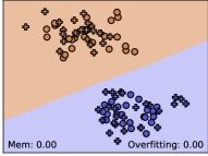
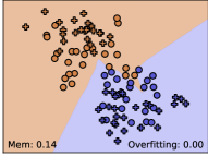
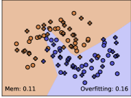
Illustration Setup. We generate a synthetic dataset for binary classification. We train a simple neural network with two hidden layers with ten neurons each. We measure overfitting using $\mathcal{G}_{err}$ and memorization using average $\mathtt{mem}$ across all data records in $\mathcal{D}_{tr}$. We depict the relationships between overfitting and memorization in Figure 2.

Illustration. In Figure 2 (a), we assume that data records in $\mathcal{D}_{tr}$ and $\mathcal{D}_{te}$ are linearly separable and drawn from similar distributions. To illustrate overfitting without memorization (Figure 2 (b)), we introduce noise to data records in $\mathcal{D}_{te}$ so that some of them cross the decision boundary. Conversely, for memorization without overfitting (Figure 2 (c)), we add noise to $\mathcal{D}_{tr}$ to bring the classes closer to the decision boundary, while still maintaining linear separability in $\mathcal{D}_{te}$. Finally, to illustrate both overfitting and memorization (Figure 2 (d)), we introduce noise to both $\mathcal{D}_{tr}$ and $\mathcal{D}_{te}$, simulating a scenario where $\mathcal{D}_{te}$ does not precisely match the distribution of $\mathcal{D}_{tr}$ for overfitting, while data records in $\mathcal{D}_{tr}$ belonging to different classes are located close to one another which are then memorized.

Relationship Cases. We describe four cases on whether overfitting and memorization occur: (a) no overfitting and no memorization (case C1), (b) overfitting but no memorization (case C2), (c) no overfitting but memorization (case C3), and (d) both overfitting and memorization (case C4).

(a) No overfitting, no memorization

(b) Overfitting, no memorization

(c) Memorization, no overfitting

(d) Overfitting, memorization

Figure 1: Relationship between overfitting and memorization: Average $\mathtt{mem}$ across all data records in $\mathcal{D}_{tr}$ and overfitting ($\mathcal{G}_{err}$) are at the bottom. Circles indicate $\mathcal{D}_{tr}$ data records, and crosses indicate $\mathcal{D}_{te}$ data records.

1. No overfitting and no memorization (Figure 2(a)) when data records in $\mathcal{D}_{tr}$ and $\mathcal{D}_{te}$ are linearly separable. Hence, $f_{\theta}$ perfectly fits $\mathcal{D}_{tr}$ and generalizes to $\mathcal{D}_{te}$ ($\mathcal{G}_{err}=0$). Further, data records in $\mathcal{D}_{tr}$ are far from the decision boundary, making them leave-one-out stable ($\mathtt{mem}$=0).

2. Overfitting but no memorization (Figure 2(b)) when $\mathcal{D}_{tr}$ is linearly separable but $\mathcal{D}_{te}$ is not. Here, $f_{\theta}$ perfectly fits $\mathcal{D}_{tr}$ but does not generalize to $\mathcal{D}_{te}$. Additionally, data records in $\mathcal{D}_{tr}$ are far from the decision boundary making them leave-one-out stable ($\mathtt{mem}$=0).

3. No overfitting but memorization (Figure 2(c)) where data records in $\mathcal{D}_{tr}$ and $\mathcal{D}_{te}$ are reasonably separable resulting in $\mathcal{G}_{err}=0$. However, with data records in $\mathcal{D}_{tr}$ being close to the decision boundary, we observe a high $\mathtt{mem}$.

4. Overfitting and memorization (Figure 2(d)) where $f_{\theta}$ both overfits to $\mathcal{D}_{tr}$, i.e., $f_{\theta}$ fits $\mathcal{D}_{tr}$ perfectly but does not generalize to $\mathcal{D}_{te}$, and memorizes some data records in $\mathcal{D}_{tr}$, i.e., they are not leave-one-out stable. In real-world applications, where $\mathcal{D}_{tr}$ and $f_{\theta}$ are complex, C4 is observed. Hence, hereafter we focus only on C4.

3.4 Overfitting and Memorization

Overfitting and memorization are distinct and occur independent of each other. We present four cases based on the presence or absence of overfitting and memorization in a model to illustrate the relation between them (Figure 2). We use a synthetic dataset for binary classification and train a simple neural network with two hidden layers with ten neurons each. We measure overfitting using $\mathcal{G}_{err}$ and memorization using average $\mathtt{mem}$ across all $\mathcal{D}_{tr}$ data records.

(a) No overfitting, no memorization

(b) Overfitting, no memorization

(c) Memorization, no overfitting

(d) Overfitting, memorization

Figure 2: Relationship between overfitting and memorization: Average $\mathtt{mem}$ across all data records in $\mathcal{D}_{tr}$ and overfitting ($\mathcal{G}_{err}$) are at the bottom. Circles indicate $\mathcal{D}_{tr}$ data records, and crosses indicate $\mathcal{D}_{te}$ data records.

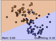
Figure 2(a) is when data records in $\mathcal{D}_{tr}$ and $\mathcal{D}_{te}$ are linearly separable. Hence, $f_{\theta}$ perfectly fits $\mathcal{D}_{tr}$ and generalizes to $\mathcal{D}_{te}$ ($\mathcal{G}_{err}=0$). Further, data records in $\mathcal{D}_{tr}$ are far from the decision boundary ($\mathtt{mem}$=0). Figure 2(b) is when $\mathcal{D}_{tr}$ is linearly separable but $\mathcal{D}_{te}$ is not ($\mathcal{G}_{err}>0$). However, data records in $\mathcal{D}_{tr}$ are far from the decision boundary ($\mathtt{mem}$=0). Figure 2(c) is when data records in $\mathcal{D}_{tr}$ and $\mathcal{D}_{te}$ are reasonably separable resulting in $\mathcal{G}_{err}=0$. However, with $\mathcal{D}_{tr}$ data records being close to the decision boundary, we observe a high $\mathtt{mem}$. Figure 2(d) is where $f_{\theta}$ both overfits to $\mathcal{D}_{tr}$, i.e., $f_{\theta}$ fits $\mathcal{D}_{tr}$ perfectly but does not generalize to $\mathcal{D}_{te}$, and memorizes some data records in $\mathcal{D}_{tr}$, i.e., they are not leave-one-out stable. This is generally seen in real-world applications, where $\mathcal{D}_{tr}$ and $f_{\theta}$ are complex. Hence, hereafter we focus only on this setting.

4 Understanding Unintended Interactions

We now show how factors influencing overfitting and memorization relate to defenses (Section 4.1) and risks (Section 4.2), summarizing in Table II. We then survey unintended interactions explored in prior work, and situate them within our framework (Section 4.3). Finally, we suggest a guideline to help conjecture such interactions using our framework (Section 4.4).

4.1 Revisiting Defenses for ML

We explore how the effectiveness of different defenses correlates with different factors. We also indicate whether a defense degrades accuracy (▼) or not (♒).

RD1 (Adversarial Training). $f_{\theta}$ learns spurious attributes which are essential for achieving high accuracy and low $\mathcal{G}_{err}$. However, this makes $f_{\theta}$ susceptible to evasion [73]. $f^{rob}_{\theta}$ is compelled to learn stable attributes [161, 73]. This improves robustness but with higher $\mathcal{G}_{err}$ and an accuracy drop (▼) [73]. More training data can reduce overfitting [161]. Increasing the tail length, lowers robustness for the tail classes [71, 16]. Also, RD1 includes a regularization term to minimize the maximum loss from adversarial examples which results in a smoother curvature [102]. This creates an explicit trade-off between generalization and robustness [151]. This is accompanied with an increase in the distance of $\mathcal{D}_{tr}$ data records to the decision boundary [176]. Further, $f^{rob}_{\theta}$ exhibits higher distinguishability between predictions on data records inside and outside $\mathcal{D}_{tr}$ [144]. Finally, $f^{rob}_{\theta}$ should have high capacity to learn adversarial examples [102].

RD2 (Outlier Removal). Outliers are identified by measuring the influence of memorized data records on observables [81]. A longer tail increases the number of memorized outliers making their detection easy [166]. Some of these outliers contribute to $f_{\theta}$’s accuracy [47, 48, 20]. Thus, removing such outliers increases overfitting in $f^{outrem}_{\theta}$ which results in an accuracy drop (▼) [81, 80, 46, 79].

RD3 (Watermarking). Ideally, $f^{wm}_{\theta}$ should maintain $\mathcal{G}_{err}$ similar to $f_{\theta}$. In practice, $f^{wm}_{\theta}$ incurs an accuracy drop (▼) [3, 152, 98]. A long tail enables stealthier watermarks from tail classes [96]. Lower distinguishability in observables for watermarks between $f_{\theta}$ and $f^{der}_{\theta}$, but distinct from independently trained models, helps identifying $f^{der}_{\theta}$ [3]. High model capacity aids memorizing the watermarks [3].

RD4 (Fingerprinting). There is no explicit impact on overfitting, memorization, or accuracy (♒) as RD4 does not require retraining. A lower distinguishability in fingerprints between $f_{\theta}$ and $f^{der}_{\theta}$, but distinct from independently trained models, is preferred for effectively identifying $f^{der}_{\theta}$ [165, 97]. The effectiveness of fingerprints relies on $f_{\theta}$’s overfitting and memorization. For instance, dataset inference [106] hinges on the distinguishability of observables between data records inside and outside $\mathcal{D}_{tr}$, for both $f_{\theta}$ and $f^{der}_{\theta}$. This helps identify if they share overlapping $\mathcal{D}_{tr}$. Similarly, fingerprints based on adversarial examples rely on $f_{\theta}$’s generalization for transferring adversarial examples to $f^{der}_{\theta}$ [97, 106, 21, 122, 167]. For effective transfer, a lower distance to the boundary is preferred [97, 122, 21].

PD1 (Differential Privacy). Memorization of data records is reduced by lowering their influence on observables with PD1. $f^{dp}_{\theta}$ is compelled to learn stable attributes as evident by better privacy guarantees in causal models [155]. Also, adding noise to gradients regularizes $f^{dp}_{\theta}$ which curbs overfitting but with an accuracy drop (▼) [2, 77, 128]. This reduces distinguishability in observables for data records inside and outside $\mathcal{D}_{tr}$ [2], and decreases the distance of $\mathcal{D}_{tr}$ data records to the boundary [162]. Also, PD1 reduces the curvature smoothness [162, 18], and lower privacy for tail classes [150, 11]. Low capacity leads to reasonable privacy, without significant accuracy drop [135].

FD1 (Group Fairness). For fairness via in-processing algorithms, the regularization term explicitly creates a trade-off between fairness and accuracy [187, 164], exacerbating overfitting with a drop in $f^{fair}_{\theta}$’s accuracy (▼) [124, 129, 187, 164]. This reduces distinguishability in observables across subgroups [1, 189]. Further, $f^{fair}_{\theta}$ prioritizes learning stable attributes which do not overlap with sensitive attributes [114, 1]. For equitable behaviour, $f^{fair}_{\theta}$ memorizes some data records in minority subgroups, thereby decreasing their distance to the boundary [29, 160].

FD2 (Explanations). There is no explicit impact on overfitting, memorization, or accuracy (♒) as FD2 does not require retraining. More attributes increase the dimensions of the explanations, and reduce the influence of individual attributes which affects the quality of FD2 [137]. Also, FD2 exhibits distinguishability across subgroups [44]. The quality of explanations is tied to $f_{\theta}$’s overfitting: they exhibit better approximation for data records in $\mathcal{D}_{tr}$ compared to $\mathcal{D}_{te}$ [137]. Therefore, FD2 exhibits higher distinguishability between data records inside and outside $\mathcal{D}_{tr}$ [137].

We summarize the relation between effectiveness of defenses with factors in Table II. For a defense <d> and a factor <f>, $\uparrow$ indicates <d> positively correlates with <f>; $\downarrow$ indicates a negative correlation.

4.2 Revisiting Risks in ML

We now discuss different factors and how it correlates with the susceptibility on different risks.

TABLE II: Summary of correlation between effectiveness of a defense <d> and susceptibility to a risk <r> with a factor <f>:
$\uparrow$ indicates <d> or <r> positively correlates with <f>; $\downarrow$ indicates a negative correlation.

Defences (<$\uparrow$ or $\downarrow$>, <f>)

Risks (<$\uparrow$ or $\downarrow$>, <f>)

RD1 (Adversarial Training): • D1 $\uparrow$, $|\mathcal{D}_{tr}|$ [161] • D2 $\downarrow$, tail length [71, 16] • D4 $\uparrow$, priority for learning stable attributes [161] • O1 $\uparrow$, curvature smoothness [102] • O2O2.1 $\uparrow$, distinguishability in data records inside and outside $\mathcal{D}_{tr}$ [144] • O3 $\uparrow$, distance to boundary for most $\mathcal{D}_{tr}$ data records [176] • M1 $\uparrow$, model capacity [102] RD2 (Outlier Removal): • D2 $\uparrow$, tail length [166] RD3 (Watermarking): • D2 $\uparrow$, tail length [96] • O2O2.3 $\downarrow$, distinguishability in observables for watermarks between $f_{\theta}$ and $f^{der}_{\theta}$, but distinct from independent models [3] • M1 $\uparrow$, model capacity [3] RD4 (Fingerprinting): • O2O2.3 $\downarrow$, distinguishability in observables for fingerprints between $f_{\theta}$ and $f^{der}_{\theta}$, but distinct from independent models [165, 97] • O3 $\downarrow$, distance of $\mathcal{D}_{tr}$ data records to boundary [97, 122, 21] PD1 (Differential privacy): • D2 $\downarrow$, tail length [11, 150] • D4 $\uparrow$, priority for learning stable attributes [155] • O1 $\downarrow$, curvature smoothness [162, 18] • O2O2.1 $\downarrow$, distinguishability for data records inside and outside $\mathcal{D}_{tr}$ [2] • O3 $\downarrow$, distance of $\mathcal{D}_{tr}$ data records to decision boundary [162] • M1 $\downarrow$, model capacity [135] FD1 (Group Fairness): • D4 $\uparrow$, priority for learning stable attributes [53, 114, 1] • O2O2.2 $\downarrow$, distinguishability of observables across subgroups [1, 189] • O3 $\downarrow$, distance to decision boundary for most $\mathcal{D}_{tr}$ data records [160] FD2 (Explanations): • D3 $\downarrow$, number of input attributes [137] • O2O2.1 $\uparrow$, distinguishability in data records inside and outside $\mathcal{D}_{tr}$ [137] • O2O2.2 $\uparrow$, distinguishability across subgroups [44]

R1 (Evasion): • D2 $\uparrow$, tail length [173, 91] • O1 $\downarrow$, curvature smoothness [102] • O3 $\downarrow$, distance of $\mathcal{D}_{tr}$ data records to boundary [162] R2 (Poisoning): • D2 $\uparrow$, tail length [120, 17, 96] • M1 $\uparrow$, model capacity [3] R3 (Unauthorized Model Ownership): • M1 $\downarrow$, model capacity [117, 88] P1 (Membership Inference): • D1 $\downarrow$, |$\mathcal{D}_{tr}$| [184, 136] • D2 $\uparrow$, tail length [25, 24] • D4 $\downarrow$, priority for learning stable attributes [103, 155] • O2O2.1 $\uparrow$, distinguishability for data records inside and outside $\mathcal{D}_{tr}$ [136] • O3 $\downarrow$, distance to decision boundary [137] • M1 $\uparrow$, model capacity [144, 45] P2 (Data Reconstruction): • D2 $\uparrow$, tail length [171] • D3 $\downarrow$, number of input attributes [51] • O2O2.1 $\uparrow$, distinguishability for data records inside and outside $\mathcal{D}_{tr}$ [199, 115] • O2O2.2 $\uparrow$, distinguishability in observables across subgroups [180] P3 (Attribute Inference): • D2 $\uparrow$, tail length [78] • D4 $\downarrow$, priority for learning stable attributes [103, 143] • O2O2.2 $\uparrow$, distinguishability in observables across subgroups [1] P4 (Distribution Inference): • D2 $\uparrow$, tail length [30, 105] • D4 $\uparrow$, priority for learning stable attributes [148] • O2O2.1 $\uparrow$, distinguishability in observables between datasets [149, 148] • M1 $\uparrow$, model capacity [30] F (Discriminatory behaviour): • D2 $\uparrow$, tail length [110] • O2O2.2 $\uparrow$, distinguishability in observables across subgroups [189]

R1 (Evasion). Longer tails increase R1: adversarial examples from tail classes are more effective [173, 91]. Lower curvature smoothness makes it easier to generate adversarial examples [102]. Further, data records close to $f_{\theta}$’s decision boundary require smaller perturbations to induce misclassification [85, 31]. Hence, R1 risk decreases for data records farther away from the boundary [162]. When overfitting and memorization are pronounced, the decision boundary is more complex and bigger, making R1 easier [31].

R2 (Poisoning). Longer tail increases R2 as the poisons from tail classes are more discreet [120, 17, 96]. Following watermarking literature which use poisons, the effectiveness of poisons is higher with larger $f_{\theta}$ capacity due to their better memorization [3].

R3 (Unauthorized Model Ownership). Whitebox model theft does not explicitly change overfitting or memorization. Henceforth, we focus only on blackbox model extraction. R3 is less successful if $f_{\theta}$ overfits or memorizes: accuracy of $f_{\theta}$ is lower and consequently, labels from $f_{\theta}$ for training $f^{der}_{\theta}$ are of a bad quality. Hence, $f^{der}_{\theta}$ has low accuracy [95]. Also, for a given $f^{der}_{\theta}$, increasing $f_{\theta}$’s capacity will decrease R3 [88, 117].

P1 (Membership Inference). Overfitting is correlated with an increase in P1. Hence, P1 decreases with larger $|\mathcal{D}_{tr}|$ as it increases generalization [184, 136]. Further, when $f_{\theta}$ prioritizes learning stable attributes, P1 decreases due to better generalization [103, 155]. Also, a higher distinguishability between data records inside and outside $\mathcal{D}_{tr}$, increases P1 [136, 184, 70]. Memorized data records exhibit a higher influence on observables, rendering them more susceptible to P1 [46, 24]. Hence, longer tail increases memorized outliers thereby increasing their susceptibility [25, 24]. Also, data records located farther from the decision boundary, with low memorization, are less susceptible to P1 [137]. Finally, increasing $f_{\theta}$’s capacity amplifies the memorization of $\mathcal{D}_{tr}$, which increases P1 [144, 45].

P2 (Data Reconstruction). Overfitting improves reconstruction of data records in $\mathcal{D}_{tr}$ [115]. Higher distinguishability between records inside and outside $\mathcal{D}_{tr}$, increases P2 [199]. Memorization amplifies the influence of data records on observables, leading to better reconstruction [142, 200, 172, 171]. P1 is higher for outliers from tail classes [171]. Further, more input attributes reduces accurate reconstruction of inputs [51]. Finally, higher distinguishability in observables across subgroups increases P2 [180].

P3 (Attribute Inference). Memorization of sensitive attributes is likely to increase P3 [157]. Hence, longer tail increases memorized outliers, increasing their susceptibility [78]. Prioritizing learning stable attributes decreases P3 [103, 143]. Higher distinguishability across subgroups increases P3 [1]. Notably, overfitting has no discernible impact on this risk [95].

P4 (Distribution Inference). Empirical evidence suggests that overfitting reduces P4, although the reason remains unexplained [148, 30]. Tail length correlates with P4 [30, 105]. Prioritizing stable attributes amplifies the risk because stable attributes are the same as the distributional property being inferred [148]. Higher distinguishability in observables across datasets with different distributional properties, increases P4 [149, 148]. Finally, increasing $f_{\theta}$’s capacity, without overfitting, increases P4 [30].

F (Discriminatory Behaviour). Overfitting makes bias prominent as evident by the accuracy disparity between minority and majority subgroups [177]. Increased memorization of minority subgroups contributes to their discrimination [29]. Longer tails increase memorized outliers, worsening F [110]. Increase in distinguishability of observables across subgroups correlates with increase in F [189, 1].

Table II summarizes the above discussion. For a risk <r> and a factor <f>, $\uparrow$ indicates <r> positively correlates with <f>; $\downarrow$ indicates a negative correlation.

4.3 Surveying Unintended Interactions

TABLE III: Unintended interactions between defenses with different risks. Type of interaction: ●$\rightarrow$ risk increases; ●$\rightarrow$ risk decreases; ●$\rightarrow$ unexplored. We indicate exceptions to these under “References” and discuss them in the text. Underlying factors: ● $\rightarrow$ empirical; ☉ $\rightarrow$ theoretical and ○ $\rightarrow$ conjectured. Under O2, we write O2O2.1, O2O2.2, and O2O2.3 as 1, 2, and 3 respectively. We mark the factors evaluated for conjectured interactions as ⚹ (See Section 5).

Defenses	Risks		OVFT	Memorization					Both		References
			D1	D2	D3	D4	O1	O2	O3	M1
RD1 (Adversarial Training)	R1 (Evasion)	●		●			●		●	●	[193, 102, 91, 173]
	R2 (Poisoning)	●									[170, 153]
	R3 (Unauthorized Model Ownership)	●	○								[86] ([95]: ●)
	P1 (Membership Inference)	●	☉, ●					1: ●		●	[144, 67]
	P2 (Data Reconstruction)	●				○				●	[195, 111]
	P3 (Attribute Inference)	●
	P4 (Distribution Inference)	●				○					[148]
	F (Discriminatory Behaviour)	●		☉, ●							[16, 36, 71, 99]
RD2 (Outlier Removal)	R1 (Evasion)	●									[59]
	R2 (Poisoning)	●									[154]
	R3 (Unauthorized Model Ownership)	●
	P1 (Membership Inference)	●		●							[25, 46]
	P2 (Data Reconstruction)	●
	P3 (Attribute Inference)	●		●							[78]
	P4 (Distribution Inference)	●
	F (Discriminatory Behaviour)	●	●	○							[134]
RD3 (Watermarking)	R1 (Evasion)	●
	R2 (Poisoning)	●		○							[133, 3, 194, 93]
	R3 (Unauthorized Model Ownership)	●		○				3: ●	●		[152, 3, 98]
	P1 (Membership Inference)	●		○				1: ●	●		[157, 33]
	P2 (Data Reconstruction)	●		○				1: ●	●		[157]
	P3 (Attribute Inference)	●		○				2: ●	●		[157]
	P4 (Distribution Inference)	●	☉, ●	○				1: ●	●	●	[30, 105]
	F (Discriminatory Behaviour)	●		○							[96]
RD4 (Fingerprinting)	R1 (Evasion)	●						3: ●	●		[97, 21, 122]
	R2 (Poisoning)	●
	R3 (Unauthorized Model Ownership)	●		●				3: ●	●		[202, 165, 106, 97]
	P1 (Membership Inference)	●							●		[106]
	P2 (Data Reconstruction)	●
	P3 (Attribute Inference)	●
	P4 (Distribution Inference)	●
	F (Discriminatory Behaviour)	●
PD1 (Differential Privacy)	R1 (Evasion)	●					●		●		[162, 18]
	R2 (Poisoning)	●									[76, 100, 69]
	R3 (Unauthorized Model Ownership)	●
	P1 (Membership Inference)	●				☉, ●		1: ●			[77, 128, 95, 72]
	P2 (Data Reconstruction)	●						1: ●			[182, 145]
	P3 (Attribute Inference)	●						2: ○			[95]
	P4 (Distribution Inference)	●						●			[9, 148] ([148]: ●)
	F (Discriminatory Behaviour)	●		○					●		[11, 50, 158, 188]
FD1 (Group Fairness)	R1 (Evasion)	●					●		☉, ●		[160]
	R2 (Poisoning)	●									[141, 28, 163, 109]
	R3 (Unauthorized Model Ownership)	●	○
	P1 (Membership Inference)	●	●						●	●	[29]
	P2 (Data Reconstruction)	●			⚹			2: ⚹			Our conjecture: ●
	P3 (Attribute Inference)	●						2:☉,●			[1] ([49]: ●)
	P4 (Distribution Inference)	●	●								[148]
	F (Discriminatory Behaviour)	●	●					2:●			[83, 189, 4, 125]
FD2 (Explanations)	R1 (Evasion)	●									[198, 126]
	R2 (Poisoning)	●			●		☉, ●			●	[192, 14, 68, 139]
	R3 (Unauthorized Model Ownership)	●									[168, 5, 126]
	P1 (Membership Inference)	●	●		●			1: ●	●	●	[137, 121, 126]
	P2 (Data Reconstruction)	●		☉, ●	●						[137, 201]
	P3 (Attribute Inference)	●						2: ○			[44]
	P4 (Distribution Inference)	●			⚹			1: ⚹		⚹	Our Conjecture: ●
	F (Discriminatory Behaviour)	●		●	●					●	[12, 38] ([87, 132]: ●)

We now survey various unintended interactions reported in the literature and situate them within our framework (Table III). We mark the interaction between <d> and <r> as ● if “an increase (decrease) in effectiveness of <d> correlates with an increase (decrease) in <r>” and ● if “an increase (decrease) in effectiveness of <d> correlates with a decrease (increase) in <r>”. We use the different factors from Table I to gain a more nuanced understanding of the interactions. We mark a factor with ● if there are empirical results regarding its influence, ☉ if there are theoretical results and ○ if it is only conjectured. In some cases, there are exceptions to the nature of the interaction depending on the threat model. We indicate them under “References” along with their relevant citation(s) in Table I and discuss them in the text.

RD1 (Adversarial Training)

● R1 (Evasion) is less effective with RD1 which is specifically designed to resist adversarial examples [102, 193, 92]. Using the min-max objective function increases the curvature smoothness which reduces the possibility of generating adversarial examples [102]. Further, RD1 pushes the decision boundary away from the data records [193]. Also, $f^{rob}_{\theta}$ requires a high capacity to learn a complex decision boundary to fit adversarial examples [102]. Longer tail increases the effectiveness of adversarial examples from the tail classes despite using RD1 [91, 173].

● R2 (Poisoning) can be effective with RD1 [170]. Recall that $f^{rob}_{\theta}$ is forced to learn stable attributes. Hence, it might seem that poisons, generated by manipulating spurious attributes, does not affect $f^{rob}_{\theta}$’s predictions [153]. However, Wen et al. [170] design poisons to degrade $f^{rob}_{\theta}$’s accuracy by manipulating the stable attributes.

● R3 (Unauthorized model ownership) can be more prevalent as model theft of $f^{rob}_{\theta}$ is easier than $f_{\theta}$ [86]. However, no reasons were explored. We conjecture that since $f^{rob}_{\theta}$ has uniform predictions on neighboring data records [82, 156, 102, 92], hence, $f^{der}_{\theta}$ requires fewer queries compared to $f_{\theta}$. The above interaction assumes $\mathcal{A}dv$ is a malicious suspect. For a malicious accuser, RD1 can mitigate false claims [94], which decreases R3 (●).

● P1 (Membership inference) is easier with RD1 [144, 67]. Recall that RD1 modifies $f^{rob}_{\theta}$’s decision boundary to memorize adversarial examples in $\mathcal{D}_{tr}$ [144]. This increases the influence of some records on observables. Consequently, the distinguishability between data records inside and outside $\mathcal{D}_{tr}$ is higher [144]. Hence, P1 increases. Hayes et al. [67] provably show that increasing $|\mathcal{D}_{tr}|$ lowers overfitting and hence, reduces P1. Further, P1 increases with $f^{rob}_{\theta}$’s capacity due to higher memorization.

● P2 (Data reconstruction) is easier with RD1 [195, 111]: $f^{rob}_{\theta}$ has interpretable gradients [127], which enhances the quality of reconstruction. Further, consistent attributes across inputs, are easier to reconstruct.Finally, lower $f^{rob}_{\theta}$’s capacity increases P2 [195].

● P3 (Distribution inference) is easier as $f^{rob}_{\theta}$ tends to learn stable attributes which matches with distributional properties being inferred [148]. However, increasing $\epsilon_{rob}$ reduces P3 as $f^{rob}_{\theta}$’s accuracy decreases.

● F (Discriminatory behaviour) increases with RD1 as evident from the accuracy disparity of $f^{rob}_{\theta}$ across different classes [71, 16, 36]. Longer tail contributes to the tail classes having lower robustness [71, 16]. Also, increasing $\epsilon_{rob}$, increases the class-wise disparity [99]. Empirically, $|\mathcal{D}_{tr}|$, $f^{rob}_{\theta}$’s capacity, type of $\mathcal{D}_{tr}$ (e.g., images, tabular), and $f^{rob}_{\theta}$’s architecture and optimization algorithms do not influence the interaction [71, 16].

RD2 (Outlier Removal)

● R1 (Evasion) is less effective with RD2 [59]. Adversarial examples are outliers compared to $\mathcal{D}_{tr}$’s distribution which can detected before passing them as inputs [59].

● R2 (Poisoning) is less effective with RD2 [154, 120]. Poisons have a different distribution from $\mathcal{D}_{tr}$ and can be detected and removed as outliers during pre-processing [120]. During training, the influence of outliers, often correspond to poisons, on observables can be minimized [17].

● P1 (Membership inference) is arguably worse with RD2 followed by retraining [25]. Memorized outliers are more susceptible to membership inference. However, after removing these outliers, $f^{outrem}_{\theta}$ memorizes other data records making them more susceptible than before [25]. Varying $|\mathcal{D}_{tr}|$, $f^{outrem}_{\theta}$’s capacity, or the number of duplicates in $\mathcal{D}_{tr}$ does not have any impact on the risk [25].

● P3 (Attribute inference) is more effective as retraining after removal of memorized outliers constituting the long-tail of $\mathcal{D}_{tr}$, makes new data records susceptible [78].

● F (Discriminatory behaviour) increases as outliers could constitute a statistical minority. This exacerbates bias against minorities by excessively identifying them as outliers [134]. On increasing $|\mathcal{D}_{tr}|$, more minority data records are classified as outliers further exacerbating the bias [134].

RD3 (Watermarking)

● R2 (Poisoning) is used by most watermarking schemes thereby requiring $f_{\theta}$ to be susceptible to it [133, 3, 194, 93]. These schemes inject data records closer to outliers for memorization by $f_{\theta}$. Hence, longer tails can help generate effective and discreet poisons as watermarks.

● R3 (Unauthorized model ownership) can be detected with RD3 [152, 3, 98]. $f^{wm}_{\theta}$ should have enough capacity to memorize watermarks. Therefore, increasing capacity can improve effectiveness of watermarking [98]. Also, longer tails help generate more discreet watermarks.

● P1 (Membership inference), P2 (Data reconstruction), P3 (Attribute inference), P4 (Distribution inference) do not have any prior evaluations with watermarks. However, prior work has explored stealthy poisoning where mislabeled data records are added to $\mathcal{D}_{tr}$ to increase different privacy risks without an accuracy drop [157, 33, 30, 105]. We liken this form of poisoning to RD3 [133, 3, 194, 93], and use their observations to justify different interactions.

We conjecture that adding watermarks from tail classes, similar to poisoning, will increase privacy risks. Hence, a longer tail is likely to increase different privacy risks. Further, memorization of watermarks increases their influence on observables. This increases the distinguishability in observables across datasets, subgroups, and models. Moreover, the decision boundary is more complex, consequently increasing the susceptibility of outliers closer to the decision boundary [157, 33]. For distribution inference, the risk increases with lower capacity, and higher $|\mathcal{D}_{tr}|$ [30, 105].

● F (Discriminatory behaviour) could worsen with watermarking schemes which rely on adding bias to $\mathcal{D}_{tr}$ [96]. Watermarks (with incorrect labels) belonging to the tail classes are more effectively memorized for ownership verification [96, 28, 75]. Hence, increasing the tail length is likely to increase the effectiveness of watermarks.

RD4 (Fingerprinting)

● R1 (Evasion) can be used for fingerprinting with adversarial examples, necessitating $f_{\theta}$’s susceptibility to this risk [97, 122, 21]. Hence, when $f_{\theta}$ is robust against evasion, fingerprints are less effective [97]. Such fingerprints require $\mathcal{D}_{tr}$ records to be closer to class boundaries [21]. Further, overfitting and memorization make the decision boundary complex, which helps generate fingerprints. To transfer these fingerprints from $f_{\theta}$ to $f^{der}_{\theta}$, the distinguishability between their observables should be low but distinct from independent models [97, 122, 21].

● R3 (Unauthorized model ownership) can be detected using fingerprints. Fingerprints based on adversarial examples are closer to the outliers in the tail classes of $\mathcal{D}_{tr}$’s distribution. Unique intermediate activations for a given input can also be used as a fingerprint which have low distinguishability between $f_{\theta}$ and $f^{der}_{\theta}$ but distinct from independent models [165].

● P1 (Membership inference) can be used to construct fingerprints which relies $f_{\theta}$ being susceptible to it. Dataset inference [106] uses a weak membership inference attack to identify $f_{\theta}$’s decision boundary, that constitute its fingerprint. Specifically, it distinguishes between the distribution of distances of data records in $\mathcal{D}_{tr}$ and any other independent dataset to the decision boundary, and not any individual data records.

PD1 (Differential Privacy)

● R1 (Evasion) is easier for $f^{dp}_{\theta}$. DPSGD reduces the distance between $\mathcal{D}_{tr}$ records and decision boundaries making it easier to generate adversarial examples [162]. Also, training with DPSGD results in a less smooth curvature which can can potentially increase R1 [162, 113, 18, 41]. $f^{dp}_{\theta}$ creates a false sense of robustness via gradient masking, i.e., modifying the gradients to be useless for gradient based evasion (as observed in [162]). However, $f^{dp}_{\theta}$ is still susceptible to non-gradient evasion.

● R2 (Poisoning) can be more effective against $f^{dp}_{\theta}$. Prior works have suggested that R2 decreases as PD1 reduces their influence on the observables [69, 100]: DPSGD constrains gradient magnitudes which enhances $f^{dp}_{\theta}$’s robustness against poisons. However, it has been shown that the choice of hyperparameters (e.g., noise multiplier, gradient clipping) are the reason for an improvement in robustness [76]. More investigation is required to understand the root cause of this interaction.

● P1 (Membership inference) is less effective on $f^{dp}_{\theta}$ due to PD1’s regularizing effect as evident from low $\mathcal{G}_{err}$ [2]. This reduces the distinguishability between data records inside and outside $\mathcal{D}_{tr}$ [2, 77, 95]. Further, PD1 provably bounds P1 for i.i.d. data [77, 128]. Prioritizing causal attributes gives a higher privacy guarantee while reducing the risk to P1 [155]. However, PD1’s guarantee does not hold for P1 on non-i.i.d data [72]. Also, duplicates in $\mathcal{D}_{tr}$ weaken the bound and the achievable $\epsilon_{dp}$ is too high for P1.

● P2 (Data reconstruction) is less effective against $f^{dp}_{\theta}$ as PD1 reduces the distinguishability between data records inside and outside $\mathcal{D}_{tr}$ [182]. The lower quality of information available to $\mathcal{A}dv$ reduces P2.

● P3 (Attribute inference) was less effective against $f^{dp}_{\theta}$ [95], but no explanation was presented. We conjecture that PD1, by reducing the memorization of sensitive attributes and their influence on observables, reduces the distinguishability across subgroups [81].

● P4 (Distribution inference) is less effective assuming $\mathcal{A}dv$ does not know $f^{dp}_{\theta}$’s training hyperparameters to adapt the attack [148]. PD1 has a regularizing effect which reduces $f^{dp}_{\theta}$’s ability to learn $\mathcal{D}_{tr}$’s distribution. This reduces the distinguishability of observables across datasets with different distributional properties thereby reducing P4 [148]. However, if $\mathcal{A}dv$ is aware of training hyperparameters, they can adapt their attack to increase P4 (●) [148].

● F (Discriminatory behaviour) increases for $f^{dp}_{\theta}$ as evident by accuracy disparity between minority and majority subgroups [11]. This effect varies with $f^{dp}_{\theta}$’s architecture. Also, training hyperparameters (e.g., clipping and gradient noise) disproportionately affect underrepresented classes [158]. Further, longer tail results in poor privacy protection for the tail classes [150]. These data records have a high gradient norm and are closer to the decision boundary, which exacerbates the disparity [158]. Finally, lowering $\epsilon_{dp}$ makes the disparity worse [11].

FD1 (Group Fairness)

● R1 (Evasion) is easier against $f^{fair}_{\theta}$. Data records in $\mathcal{D}_{tr}$ have a smaller distance to the decision boundary making it easier to generate adversarial examples [160]. Robustness, on the other hand, is higher for data records with a larger distance to the decision boundary. Hence, the optimization for FD1 is contrary to the robustness requirement [160].

● R2 (Poisoning) is more effective against $f^{fair}_{\theta}$ [141, 28, 163, 109]. It aims to increase $f^{fair}_{\theta}$’s disparity, and differs in ways to craft poisons which include: using $f^{fair}_{\theta}$’s gradients [141], distorting $\mathcal{D}_{tr}$’s distribution [28], skewing the decision boundary [109], and maximizing the covariance between the sensitive attributes and labels [109].

● P1 (Membership inference) is more effective against $f^{fair}_{\theta}$ [29]. Memorization of some data records lowers their distance to decision boundary thereby increasing their influence on observables which increases P1 [29]. Further, P1 increases with $f^{fair}_{\theta}$’s capacity and $|\mathcal{D}_{tr}|$ assuming the fraction of minority subgroup remains the same [29]. This is assuming equalized odds as a fairness metric. It is not clear how the nature of the interaction changes for a different fairness metric (e.g., demographic parity).

● P3 (Attribute inference) is less effective. $f^{fair}_{\theta}$ has lower distinguishability in predictions across subgroups [1]. Hence, FD1 specifically with demographic parity as a constraint, can provably and empirically reduce P3 [1]. On the contrary, Ferry et al. [49] show that it is possible to infer sensitive attributes from $f^{fair}_{\theta}$ which suggests an increase in P3 (●). However, this is under a restrictive threat model where $\mathcal{A}dv$ knows the group fairness algorithm and hyperparameters to adapt their attack.

● P4 (Distribution inference) is less effective with over-sampling and under-sampling data records. However, the disparity between different subgroups increases [148]. Hence, the resistance to P4 and FD1 are in conflict.

● F (Discriminatory behaviour) is less for $f^{fair}_{\theta}$. This can be achieved by pre-processing $\mathcal{D}_{tr}$ to remove bias [83]. Also, in-processing using regularization reduces the distinguishability of predictions across subgroups to reduce disparity [189, 4]. Finally, post-processing can help calibrate the predictions to satisfy some fairness metric [125].

FD2 (Explanations)

● R1 (Evasion) is easier as FD2 uses gradients which captures $f_{\theta}$’s decision boundary. This helps generating adversarial examples, which in addition to forcing a misclassification, produces $\mathcal{A}dv$’s chosen explanation [198, 126].

● R2 (Poisoning) is easier as FD2 provides a new attack surface – $f_{\theta}$ is forced to output $\mathcal{A}dv$’s target explanations to hide its discriminatory behaviour  [192, 14, 68, 43]. Poisons shift the local optima, skew $\theta$ and $f_{\theta}$’s decision boundary [192, 68, 43, 139]. Further, R2 is more effective with more capacity and smoother curvature [14, 68, 139]. Furthermore, explanations such as saliency maps and counterfactuals, can be similarly manipulated [68, 139]. Less number of attributes reduces R2 by reducing the information available to $\mathcal{A}dv$.

● R3 (Unauthorized model ownership) is easier as FD2 provides information about $f_{\theta}$’s decision boundary [168, 5, 126]. For instance, exploiting counterfactuals results in $f^{der}_{\theta}$ with high accuracy and fidelity with fewer queries than exploiting predictions [5]. The variability in R3 increases with $\mathcal{A}dv$’s dataset size and imbalanced dataset [5]. The query efficiency can be improved by using a “counterfactual of a counterfactual” to train $f^{der}_{\theta}$ [168].

● P1 (Membership inference) is easier as FD2 leaks membership status [137, 121, 126]: explanations reflect the distance of data records to the boundary which makes them distinguishable for records inside and outside $\mathcal{D}_{tr}$. Further, P1 decreases when there are fewer attributes but increases with |$\mathcal{D}_{tr}$|, and $f_{\theta}$’s capacity [121].

● P2 (Data reconstruction) is easier with releasing FD2 [201]: explanations are a proxy for $f_{\theta}$’s sensitivity to different attribute values which allow for accurate reconstruction – the risk increases with the quality of explanations. Moreover, some algorithms release influential $\mathcal{D}_{tr}$ data records for a given prediction on some input. This allows for perfect reconstruction of $\mathcal{D}_{tr}$ specially for data with a longer tail and with fewer attributes [137].

● P3 (Attribute inference) is more effective as FD2 leaks the values of sensitive attributes [44]. The higher distinguishability across subgroups is a potential contributor.

● F (Discriminatory behaviour) can be detected using FD2 by identifying whether the relevant attributes are learnt by $f_{\theta}$ [132, 87]. This suggests that FD2 reduces F (●). However, explanations are flawed, i.e., they exhibit discriminatory behaviour across subgroups(●) [12, 38]. This is more pronounced for large capacity [38]. Also, explanation quality varies with the number of attributes [12].

4.4 Guideline: Exploring Unintended Interactions

We now present a guideline to identify the nature of an unintended interaction and the underlying factors influencing it. In Table II, we summarized statements about how a change in: 1. effectiveness of <d> correlates with a change in <f>, 2. <f>correlates with <r>. We used $\uparrow$ to identify positive correlation and $\downarrow$ for negative correlation. Hence, for a given <d> and <r> with a common factor <f_c>, we can infer how a change in effectiveness of <d> correlates with <r> using the direction of the pair of arrows that describe how each of <d> and <r> correspond to <f_c>.

Creating an exact algorithm for predicting unexplored interactions is difficult due to the intricate interplay of various factors. Therefore, we outline a guideline to make such conclusions with some expert knowledge about the nature of unintended interactions and underlying factors:

1. For a given <d> and <r>, identify <f_c>s from Table II.

2. For each <f_c>, if change in <f> on using <d> aligns with change in <r>, i.e., ($\uparrow$,$\uparrow$) or ($\downarrow$,$\downarrow$), then effectiveness of <d> corresponds to an increase in <r> (●) else <d> negatively correlates with <r> (●) for ($\uparrow$,$\downarrow$) or ($\downarrow$,$\uparrow$).

3. Consider the suggestions from all <f_c>s to conjecture the nature of the interaction. The final conclusion is: (a) common suggestion when all the <f_c> agree on it, (b) the suggestion from the dominant <f_c> determined using expert knowledge for conflicting suggestions from <f_c>s.

4. Empirically evaluate to see if other non-dominant <f>s influence the interaction.

Choosing Dominant <f> with Expert Knowledge. For risks other than R1 (evasion), R2 (poisoning) and R3 (unauthorized model ownership), we identify O2 as dominant. This is because these risks exploit some form of distinguishability in observables. Hence, any change to observables will influence the risks. Further, other factors such as D1, D2, D3, O2, and M1, though not dominant, can influence the interaction. These have to be evaluated empirically.

Guideline’s Coverage of Interactions. To see how well our guideline covers different interactions, we compare conclusions from our guideline with corresponding observations from our survey as the ground truth (Section 4). The guideline and the ground truth are consistent in most cases. We discuss a few exceptions in Section 6. Next, we use our guideline to conjecture about unexplored unintended interactions.

5 Unexplored Interactions and Conjectures

We enumerate different unexplored interactions (●in Table III) in Table IV. To demonstrate the applicability of our framework, we apply our guideline from Section 4.4 to present conjectures for two of these unexplored interactions and validate them empirically : i) Section 5.1: FD2 (explanations) and P4 (distribution inference) ii) Section 5.2: FD1 (group fairness) and P2 (data reconstruction). We mark the factors evaluated for these interactions with ⚹ in Table III. We then reflect on other unexplored interactions (Section 5.3).

TABLE IV: Unexplored interactions (● from Table III) from a defense to a risk (indicated with “➞” between them).

Defense ➞ Risk
RD1 (Adversarial Training) ➞ P3 (Attribute Inference)
RD2 (Outlier Removal) ➞ R3 (Unauthorized Model Ownership)
RD2 (Outlier Removal) ➞ P2 (Data Reconstruction)
RD2 (Outlier Removal) ➞ P4 (Distribution Inference)
RD3 Watermarking ➞ R1 (Evasion)
RD4 (Fingerprinting) ➞ R2 (Poisoning)
RD4 (Fingerprinting) ➞ P2 (Data Reconstruction)
RD4 (Fingerprinting) ➞ P3 (Attribute Inference)
RD4 (Fingerprinting) ➞ P4 (Distribution Inference)
RD4 (Fingerprinting) ➞ F (Discriminatory Behaviour)
PD1 Differential Privacy ➞ R3 (Unauthorized Model Ownership)
FD1 (Group Fairness) ➞ R3 (Unauthorized Model Ownership)
FD1 (Group Fairness) ➞ P2 (Data Reconstruction)
FD2 (Explanations) ➞ P4 (Distribution Inference)

5.1 FD1 ➞ P2

Conjecture. From Table II, we identify O2O2.2 as a common factor (<f_c>). As the arrows are in opposite directions, we conjecture that FD1 reduces P2 $\rightarrow$●. Now, we check for other factors: D3 suggests that P2 decreases anyway when there are more input attributes. Thus, we expect that the decrease due to FD1 is only evident when the number of attributes is small. Consequently, the difference in attack success between $f^{fair}_{\theta}$ and $f_{\theta}$ becomes negligible. We describe the experimental setup below.

Threat Model. We assume $x$ is sensitive and confidential. $\mathcal{A}dv$ only observes $f^{fair}_{\theta}(x)$ for some unknown confidential $x$ which are to be reconstructed. $\mathcal{A}dv$ also has access to auxiliary dataset which is split into $\mathcal{D}^{adv}_{tr}$ to train an attack decoder model ($f_{att}$) and $\mathcal{D}^{adv}_{te}$ for evaluation.

Attack Methodology. $\mathcal{A}dv$ uses $\mathcal{D}^{adv}_{tr}$ to train $f_{att}$ to map $f^{fair}_{\theta}(x)$ to $x$, minimizing the error between $f_{att}(\bar{f}^{fair}_{\theta}(x))$ and the ground truth $x$. Here, $\bar{f}^{fair}_{\theta}$ is a “shadow model” which is trained on $\mathcal{A}dv$’s auxiliary dataset to have similar functionality as $f^{fair}_{\theta}$. We give the advantage to $\mathcal{A}dv$ and assume $f^{fair}_{\theta}==\bar{f}^{fair}_{\theta}$. The attack is evaluated on $\mathcal{D}^{adv}_{te}$.

Setup. We use the CENSUS dataset which consists of attributes like age, race, education level, to predict whether an individual’s annual income exceeds 50K. We select the top $10$ attributes and consider both race and sex attributes. We use $|\mathcal{D}_{tr}|$=15470, $|\mathcal{D}^{adv}_{tr}|$=7735, and $|\mathcal{D}^{adv}_{te}|$=7735.

We train $f^{fair}_{\theta}$ with adversarial debiasing which uses an adversarial network $f_{inf}$ to infer sensitive attribute values from $f^{fair}_{\theta}(x)$ [189]. The loss from $f_{inf}$ is used to train $f^{fair}_{\theta}$ such that $f^{fair}_{\theta}(x)$ is indistinguishable.

We measure fairness by (a) checking if p%-rule is $>80\%$ as required by the regulations [186], and (b) AUC score of $f_{inf}$ to correctly infer the sensitive attribute values (fair model should have a score of $0.50$). To measure attack success, we use reconstruction loss ($l_{2}$-norm) between $x$ and $f_{att}(\bar{f}^{fair}_{\theta}(x))$ (higher the loss, less effective the attack). We use a multi-layered perceptron (MLP) for $f^{fair}_{\theta}$ with hidden layer dimensions [32, 32, 32, 1], $f_{inf}$ with [32, 32, 32, 2], and $f_{att}$ with [18, 32, 64, 128, 10].

We compare the attack success with the baseline of data reconstruction against $f_{\theta}$ with the same architecture as $f^{fair}_{\theta}$ but without group fairness.

Empirical Validation. We validate our conjecture, show the effect on distinguishability across subgroups (O2O2.2), and evaluate the influence of the number of input attributes (D3).

Nature of Interaction. We compare the reconstruction loss between $f^{fair}_{\theta}$ and $f_{\theta}$ in Table V. We confirm that training with adversarial debiasing is indeed fair (p%-rule $>80$% and AUC score $\sim$$0.50$). We observe that $f^{fair}_{\theta}$ has a higher reconstruction loss validating our conjecture.

TABLE V: Nature of Interaction. Comparison of $\mathcal{D}_{te}$ accuracy, fairness (AUC scores, p%-rule values) and reconstruction loss for $f_{\theta}$ and $f^{fair}_{\theta}$ across ten runs.
$\uparrow$: higher value is desirable and $\downarrow$: lower value is desirable.

Metric	$f_{\theta}$	$f^{fair}_{\theta}$
Acc $\uparrow$	84.40 $\pm$ 0.09	77.96 $\pm$ 0.58
AUC $\downarrow$	0.66 $\pm$ 0.00	0.52 $\pm$ 0.01
p%-rule Race $\uparrow$	46.51 $\pm$ 0.59	93.69 $\pm$ 5.60
p%-rule Sex $\uparrow$	29.70 $\pm$ 1.15	90.50 $\pm$ 6.87
ReconLoss $\uparrow$	0.85 $\pm$ 0.01	0.95 $\pm$ 0.02

Distinguishability in observables across subgroups (O2O2.2). We plot $f^{fair}_{\theta}$’s prediction distribution for race (whites as red vs non-whites as blue) and sex (males as red vs females as blue) (Figure 3).

(a) $f_{\theta}$’s Prediction Distribution

(b) $f^{fair}_{\theta}$’s Prediction Distribution

Figure 3: Distinguishability across subgroups (O2O2.2) decreases for $f^{fair}_{\theta}$.

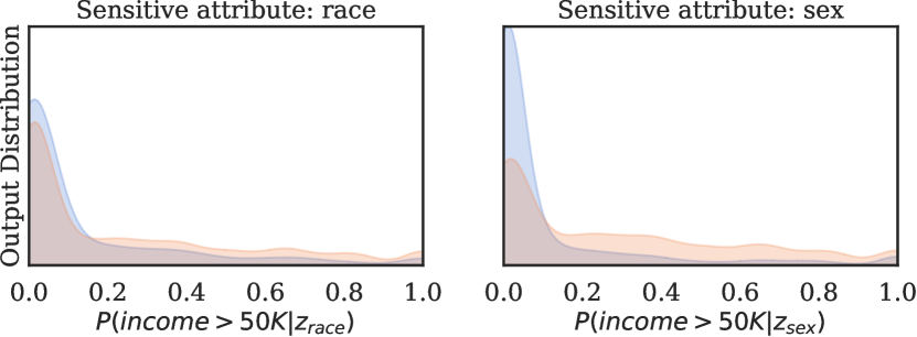
We notice that there is no income disparity between whites-non-whites and males-females for $f^{fair}_{\theta}$. Further, $f^{fair}_{\theta}$’s predictions are normalized which reduces the information available to $\mathcal{A}dv$ for successful reconstruction.

Number of Input Attributes (D3). We present the impact of the number of input attributes in Table VI. Firstly, we note that the accuracy is similar across different number of input attributes for $f^{fair}_{\theta}$ regardless of the difference in reconstruction loss. Hence, the accuracy does not impact the risk, and only the number of input attributes is the variable.

TABLE VI: Number of Input Attributes (D3). Reconstruction loss and $\mathcal{D}_{te}$ accuracy for different number of input attributes for $f_{\theta}$ and $f^{fair}_{\theta}$ (averaged across ten runs).

# Input	$f_{\theta}$		$f^{fair}_{\theta}$
Attributes	ReconLoss	Acc	ReconLoss	Acc
10	0.85 $\pm$ 0.00	84.40 $\pm$ 0.09	0.95 $\pm$ 0.02	78.96 $\pm$ 0.58
20	0.93 $\pm$ 0.03	84.72 $\pm$ 0.22	0.93 $\pm$ 0.00	80.32 $\pm$ 1.12
30	0.95 $\pm$ 0.02	84.41 $\pm$ 0.39	0.94 $\pm$ 0.00	79.50 $\pm$ 0.91

We present the reconstruction loss for a different number of input attributes {$10,20,30$}. As expected, for $10$ attributes, group fairness reduces attack success significantly (as also seen in Table V). However, increasing the number of input attributes has no significant difference in reconstruction loss between $f_{\theta}$ and $f^{fair}_{\theta}$, validating our conjecture.

5.2 FD2 ➞ P4

Conjecture. We identify O2O2.1 as <f_c>. As the arrows are the same direction, we conjecture that releasing FD2 increases P4 (●). Now, we check for other factors: the number of input attributes (D3) and model capacity (M1). For D3, increasing the number of input attributes should reduce P4 by making it harder to capture distributional properties. For M1, increasing $f_{\theta}$’s capacity should increase memorization of distributional properties, thereby increasing P4. We describe the experimental setup below.

Threat Model. We assume that on input $x$, $f_{\theta}$ outputs both explanations $\phi(x)$ and $f_{\theta}(x)$. $\mathcal{A}dv$ differentiates between $f_{\theta}$ trained on $\mathcal{D}_{tr}$ with ratio $\alpha_{1}$ vs. $\alpha_{2}$ (e.g., $50\%$ vs. $10\%$ women in $\mathcal{D}_{tr}$) by distinguishing between their respective explanations $\phi(x)^{\alpha_{1}}$, and $\phi(x)^{\alpha_{2}}$ using an ML attack model $f_{att}$. $\mathcal{A}dv$ has an auxiliary dataset which is split into $\mathcal{D}^{adv}_{tr}$ and $\mathcal{D}^{adv}_{te}$ to train and evaluate $f_{att}$.

Attack Methodology. Given two ratios, $\alpha_{1}$ or $\alpha_{2}$, $\mathcal{A}dv$ samples $\mathcal{D}^{adv}_{tr}$ to get ${}^{\alpha_{1}}\mathcal{D}^{adv}_{tr}$ and ${}^{\alpha_{2}}\mathcal{D}^{adv}_{tr}$ satisfying $\alpha_{1}$ or $\alpha_{2}$. $\mathcal{A}dv$ then trains multiple shadow models on these datasets which try to mimic $f_{\theta}$; $\mathcal{A}dv$ uses $\phi^{\prime}(x)^{\alpha_{1}}$ and $\phi^{\prime}(x)^{\alpha_{2}}$ from the shadow models to train $f_{att}$. Given $f_{\theta}$ which is trained on $\mathcal{D}_{tr}$ satisfying some unknown ratio, $\mathcal{A}dv$ uses $\phi(x)$ where $x\in\mathcal{D}^{adv}_{te}$ from $f_{\theta}$ as input to $f_{att}$ to infer if $\mathcal{D}_{tr}$’s property was $\alpha_{1}$ or $\alpha_{2}$.

Setup. We use the CENSUS dataset from Section 5.1 with $42$ input attributes. We consider different ratios of women in $\mathcal{D}_{tr}$ as our property of interest in the range $0.1-0.9$ incremented by $0.1$. Following prior work [148, 149], we set $\alpha_{1}=0.5$ while varying $\alpha_{2}$. For each value of $\alpha_{2}$, $\mathcal{A}dv$ trains $f_{att}$ to differentiate between $\alpha_{1}=0.5$ and the specific value of $\alpha_{2}$. We measure the attack success using (distribution) inference accuracy, where $50\%$ is random guess. We use an MLP with the following hidden layer dimensions: [1024, 512, 256, 128]. We use three explanation algorithms: IntegratedGradients [147], DeepLift [138, 7], and SmoothGrad [140]. For explanations, we want to evaluate if releasing explanations increases P4. Similar to interactions with explanations in prior work, we are not claiming that the risk is higher compared to exploiting predictions. Hence, we use random guess as our baseline.

Empirical Validation. We validate our conjecture and evaluate how it is influenced by the number of input attributes (D3), and model capacity (M1).

Figure 4: Nature of Interaction. Accuracy to differentiate explanations from model trained on $\mathcal{D}_{tr}$ with $\alpha_{1}$=$0.5$ and $\alpha_{2}$ $\in$ {$0.1-0.9$}.

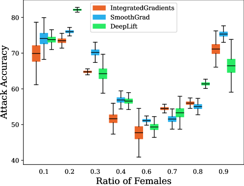
Nature of Interaction. We present the attack accuracy across different ratios and explanation algorithms in Figure 4. For all the ratios and explanation algorithms, the attack accuracy is higher than a random guess of 50%, validating our conjecture – explanations indeed leak distribution properties of $\mathcal{D}_{tr}$, and increase P4.

Number of input attributes (D3). We use an attribute selection algorithm to select the top $35$, $25$ and $15$ attributes from the original $42$ attributes. We fix $\alpha_{1}$=$0.5$ and $\alpha_{2}$=$0.1$ as it shows the highest attack accuracy (Figure 4). We present the results in Table VII.

TABLE VII: Number of input attributes (D3). Attack accuracy for $\alpha_{1}=0.5$ and $\alpha_{2}=0.1$ while varying the number of input attributes (results averaged across ten runs).

# Attributes	IntegratedGradients	DeepLift	SmoothGrad
15	81.07 $\pm$ 2.13	78.74 $\pm$ 1.66	65.40 $\pm$ 1.39
25	66.09 $\pm$ 0.95	73.64 $\pm$ 1.38	59.42 $\pm$ 1.09
35	50.43 $\pm$ 0.59	59.93 $\pm$ 2.81	56.78 $\pm$ 1.93

We confirm that increasing the number of input attributes decreases the attack success: more number of attributes decreases the memorization of each attribute thereby reducing the quality of explanations.

Model Capacity (M1). We consider four MLPs with different model capacities: “Model 1” with dimensions [128], “Model 2” with [256, 128], “Model 3” with [256,512,256], and “Model 4” is the same as before. We present the attack accuracies in Table VIII.

TABLE VIII: Model capacity (M1). Attack accuracy on explanations corresponding to $\alpha_{1}$=0.5 and $\alpha_{2}$=0.1 for different models (averaged across ten runs).

# Parameters	IntegratedGradients	DeepLift	SmoothGrad
Model 1 (5762)	47.57 $\pm$ 4.25	49.19 $\pm$ 2.75	53.26 $\pm$ 0.10
Model 2 (44162)	53.29 $\pm$ 3.65	50.86 $\pm$ 3.24	62.40 $\pm$ 0.95
Model 3 (274434	62.60 $\pm$ 2.74	67.73 $\pm$ 1.69	70.21 $\pm$ 0.73
Model 4 (733314)	69.90 $\pm$ 3.24	73.78 $\pm$ 1.03	74.09 $\pm$ 2.17

All models have an accuracy of $82.10\pm 1.17\%$ and close to perfect $\mathcal{D}_{tr}$ accuracy. Hence, neither accuracy nor $\mathcal{G}_{err}$ impacts P4. We observe that P4 increases with capacity: a higher capacity correlates with greater memorization of $\mathcal{D}_{tr}$’s distributional properties.

5.3 Other Unintended Interactions

We now reflect on other unintended interactions. RD1 (Adversarial Training) and P3 (Attribute Inference). Here, D2 and D4 are the common factors. As the arrows are in the opposite directions, both suggest a decrease in P3 (●). However, O2O2.2 is likely to be the dominant factor. Hence, the nature of this interaction will be determined by whether the distinguishability in observables across subgroups increases or decreases with RD1.

RD2 (Outlier Removal) and P2 (Data Reconstruction). Here, D1 is the common factor and the arrows are in the same direction, suggesting an increase in P2 (●). Similar to membership and attribute inference [46, 25, 78], we expect retraining without outliers will make $f^{outrem}_{\theta}$ memorize a new set of data records, thus making them more susceptible to P2.

RD2 (Outlier Removal) and P4 (Distribution Inference). D2 is the common factor which has arrows in the same direction which suggests an increase in P4 (●). Prior work has shown that adding more outliers is likely to increase P4 [30, 105]. RD2 removes outliers belonging from tail classes. We can assume that these outliers belong to minority subgroup, and outlier removal will increase the bias thereby increasing the distinguishability in observables for datasets with different properties. Hence, P4 is likely to increase.

6 Discussion

Completeness of Framework. We identified overfitting and memorization (and their underlying factors) as the causes for unintended interactions based on prior work. We do not claim them to be complete considering the complexity of ML models. However, our framework is flexible to accommodate emerging causes and factors, as well as other risks and defenses. This can be done by expanding Table II and Table III. Further, the framework can be extended to account for any exceptions in some interactions stemming from a difference in threat model (Table III).

Interactions not covered by our Guideline. There are a few interactions which are not covered by our guideline which can be addressed by extending our framework:

• RD1 (Adversarial training) ➞ R3 (Unauthorized Model Ownership); FD1 (Group fairness) ➞ R2 (Poisoning); and FD2 (Explanations) ➞ R1 (Evasion), R2 (Poisoning), R3 (Unauthorized Model Ownership): These risks do not have sufficient prior evaluation of underlying factors.

• RD1 (Adversarial Training) and PD1 (Differential Privacy) ➞ F (Discriminatory Behaviour): D2 is a common factor but it covers distribution over different classes but it does not account for subgroups. That is, data records from the tail classes may not belong to a minority subgroup.

• RD2 (Outlier Removal) ➞ R1 (Evasion), R2 (Poisoning): D2 suggests an increase in risks (●) but empirical evaluation suggests a decrease in risks (●): RD2 combines both removing outliers from $\mathcal{D}_{tr}$ and retraining. However, for R1 and R2 do not require retraining.

Minimizing Unintended Interactions. Given the factors influencing unintended interactions, practitioners can mitigate unintended interactions by exploring: 1. data augmentation (D1) 2. balanced classes with undersampling and oversampling (D2) 3. adding proxy attributes or removing redundant attributes (D3) 4. domain generalization algorithms (e.g., invariant risk minimization) [103, 66] (D4) 5. adjusting training hyperparameters (O1, O2, and O3 ) 6. experimenting with more layers, lower precision, or pruning (M1).

Applicability beyond Classifiers. Our framework extends to other models by: 1. identifying unintended interactions 2. evaluating the relation between defenses, risks, and underlying factors 3. including them in our framework for insights using our guideline. For example, in generative models where overfitting and memorization manifest as the replication of $\mathcal{D}_{tr}$ [22, 27, 23], D1 and M1 are relevant.

Related Surveys/SoKs. There are several surveys covering defenses and risks separately [118, 101, 92, 40, 70, 131, 110, 62]. None of them explore the interactions between defenses and risks. The closely related prior works are: Strobel and Shokri [146] illustrate the limited case of increased membership inference with robustness, fairness, and explanations; and Gittens et al. [57] study the interactions of different risks with DP, fairness and robustness but do not cover the factors underlying these interactions.

Interactions within Defenses. An orthogonal line of work evaluates trade-offs within defenses or designs algorithms to improve them. For instance, it is impossible to achieve group fairness and DP together [37, 6, 50]. Some prior works attempt to reconcile them by offering pareto-optimal solutions with an accuracy drop [74, 178]. Further, privacy and transparency are inherently conflicting and designing explanations with DP degrades the quality of explanations [119, 116, 63]. Conflicts also arise between watermarking with adversarial training and DP [151]. Gradients from models with adversarial training are interpretable which suggest potential alignment between transparency and robustness [127]. Furthermore, prior works have designed objective functions to reconcile adversarial training and group fairness [175]. Finally, DP over image pixels can provide certified robustness against evasion [89].

Future Work. In addition to evaluating different unexplored interactions (Table IV), a more comprehensive evaluation of different factors correlating with effectiveness of defenses and susceptibility to risks is needed (i.e., expanding Table II). Further, our framework suggests correlation and not causation. Causal reasoning can be used to establish causation between different factors with unintended interactions (e.g., [13]). Finally, the interactions are empirically evaluated, both in existing literature and our experiments in Section 5. Formally modeling these interactions and predicting their nature mathematically is for future work.

Appendix A Summary of Notations

TABLE IX: Summary of notations and their descriptions.

Notation	Description
Standard Model and Metrics
$f_{\theta}$	standard ML model (no defense)
$\theta$	$f_{\theta}$’s parameters
$\mathcal{A}$	Training algorithm
$R(\theta)$	Regularization function over $\theta$
$\lambda$	Regularization hyperparameter
$l(f_{\theta},y)$	Loss function
$f^{k}_{\theta}(x)$	$k^{th}$ layer’s output (activation)
$\mathcal{C}$	Cost function to be optimized during training
$f_{att}$	Adversary’s attack model
$\mathcal{G}_{err}$	Generalization error (train-test accuracy gap)
Data
$\mathcal{D}_{tr}$	Training dataset for $f_{\theta}$
$z_{i}=(x_{i},y_{i})$	Data record with attributes $x_{i}$ and label $y_{i}$
$\mathcal{S}$	Random subset of $\mathcal{D}_{tr}$
$|\mathcal{D}_{tr}|$	Size of $\mathcal{D}_{tr}$
$\mathcal{D}_{te}$	Test dataset
$\mathcal{D}^{adv}_{tr}$	Adversary’s dataset to train $f_{att}$
$\mathcal{D}^{adv}_{te}$	Adversary’s dataset to evaluate $f_{att}$
Defenses and Risks
$f^{rob}_{\theta}$	Robust model from adversarial training
$f^{dp}_{\theta}$	Private model from DPSGD
$f^{fair}_{\theta}$	Fair model with group fairness constrains
$f^{der}_{\theta}$	Stolen model derived from $f_{\theta}$
$x_{adv}$	Adversarial Example
$f^{outrem}_{\theta}$	Model after retraining on $\mathcal{D}_{tr}$ without outliers
$f^{wm}_{\theta}$	Model trained with watermarks
$\epsilon_{rob}$	Perturbation budget for adversarial examples
$\delta_{rob}$	Perturbation added to generate $x_{adv}$
$\epsilon_{dp}$	Privacy budget
$\delta_{dp}$	probability where privacy loss $>$ $e^{\epsilon}_{dp}$
Evaluating Conjectures
$\alpha_{1}$, $\alpha_{2}$	Distributional properties of $\mathcal{D}_{tr}$
${}^{\alpha_{1}}\mathcal{D}^{adv}_{tr}$, ${}^{\alpha_{2}}\mathcal{D}^{adv}_{tr}$	Datasets satisfying $\alpha_{1}$, $\alpha_{2}$
$\phi(x)^{\alpha_{1}}$, $\phi(x)^{\alpha_{2}}$	Explanations corresponding to $\alpha_{1}$ and $\alpha_{2}$

References

- [1] J. Aalmoes et al., “Leveraging algorithmic fairness to mitigate blackbox attribute inference attacks,” arXiv preprint arXiv:2211.10209, 2022.
- [2] M. Abadi et al., “Deep learning with differential privacy,” in CCS, 2016, p. 308–318. [Online]. Available: https://doi.org/10.1145/2976749.2978318
- [3] Y. Adi et al., “Turning your weakness into a strength: Watermarking deep neural networks by backdooring,” in USENIX Security, 2018, pp. 1615–1631. [Online]. Available: https://www.usenix.org/conference/usenixsecurity18/presentation/adi
- [4] A. Agarwal et al., “A reductions approach to fair classification,” in ICML, vol. 80, 2018, pp. 60–69.
- [5] U. Aïvodji et al., “Model extraction from counterfactual explanations,” arXiv preprint arXiv:2009.01884, 2020.
- [6] G. Alves et al., “Survey on fairness notions and related tensions,” EURO Journal on Decision Processes, 2023.
- [7] M. Ancona et al., “Towards better understanding of gradient-based attribution methods for deep neural networks,” in ICLR, 2018. [Online]. Available: https://openreview.net/forum?id=Sy21R9JAW
- [8] D. Arpit et al., “A closer look at memorization in deep networks,” in ICML, 2017, p. 233–242.
- [9] G. Ateniese et al., “Hacking smart machines with smarter ones: How to extract meaningful data from machine learning classifiers,” Int. J. Secur. Netw., vol. 10, no. 3, p. 137–150, Sep. 2015.
- [10] B. G. Atli Tekgul and N. Asokan, “On the effectiveness of dataset watermarking,” in IWSPA, 2022, p. 93–99. [Online]. Available: https://doi.org/10.1145/3510548.3519376
- [11] E. Bagdasaryan et al., “Differential privacy has disparate impact on model accuracy,” in NeurIPS, 2019, pp. 15 479–15 488.
- [12] A. Balagopalan et al., “The road to explainability is paved with bias: Measuring the fairness of explanations,” in FaccT, 2022, p. 1194–1206. [Online]. Available: https://doi.org/10.1145/3531146.3533179
- [13] T. Baluta et al., “Membership inference attacks and generalization: A causal perspective,” in CCS, 2022, p. 249–262.
- [14] H. Baniecki et al., “Fooling partial dependence via data poisoning,” in Machine Learning and Knowledge Discovery in Databases, 2023, pp. 121–136.
- [15] M. Belkin et al., “Reconciling modern machine-learning practice and the classical bias–variance trade-off,” Proc. of National Academy of Sciences, vol. 116, no. 32, pp. 15 849–15 854, 2019. [Online]. Available: https://www.pnas.org/doi/abs/10.1073/pnas.1903070116
- [16] P. Benz et al., “Robustness may be at odds with fairness: An empirical study on class-wise accuracy,” in NeurIPS Workshop on Pre-registration in ML, 2021, pp. 325–342. [Online]. Available: https://proceedings.mlr.press/v148/benz21a.html
- [17] P. Blanchard et al., “Machine learning with adversaries: Byzantine tolerant gradient descent,” in NeurIPS, 2017. [Online]. Available: https://proceedings.neurips.cc/paper/2017/file/f4b9ec30ad9f68f89b29639786cb62ef-Paper.pdf
- [18] F. Boenisch et al., “Gradient masking and the underestimated robustness threats of differential privacy in deep learning,” arXiv preprint arXiv:2105.07985, 2021.
- [19] E. Borgnia et al., “Strong data augmentation sanitizes poisoning and backdoor attacks without an accuracy tradeoff,” in ICASSP, 2021, pp. 3855–3859.
- [20] G. Brown et al., “When is memorization of irrelevant training data necessary for high-accuracy learning?” in STOC, 2021, p. 123–132.
- [21] X. Cao et al., “Ipguard: Protecting intellectual property of deep neural networks via fingerprinting the classification boundary,” in AsiaCCS, 2021, p. 14–25. [Online]. Available: https://doi.org/10.1145/3433210.3437526
- [22] N. Carlini et al., “The secret sharer: Evaluating and testing unintended memorization in neural networks,” in USENIX Security, 2019, pp. 267–284. [Online]. Available: https://www.usenix.org/conference/usenixsecurity19/presentation/carlini
- [23] ——, “Extracting training data from large language models,” in USENIX Security, 2021, pp. 2633–2650. [Online]. Available: https://www.usenix.org/conference/usenixsecurity21/presentation/carlini-extracting
- [24] ——, “Membership inference attacks from first principles,” in S&P, 2022, pp. 1897–1914.
- [25] ——, “The privacy onion effect: Memorization is relative,” in NeurIPS, 2022. [Online]. Available: https://openreview.net/forum?id=ErUlLrGaVEU
- [26] ——, “Quantifying memorization across neural language models,” arXiv preprint arXiv:2202.07646, 2022.
- [27] ——, “Extracting training data from diffusion models,” in USENIX Security, 2023.
- [28] H. Chang et al., “On adversarial bias and the robustness of fair machine learning,” 2020.
- [29] H. Chang and R. Shokri, “On the privacy risks of algorithmic fairness,” in EuroS&P, 2021, pp. 292–303.
- [30] H. Chaudhari et al., “Snap: Efficient extraction of private properties with poisoning,” in S&P, 2023, pp. 400–417. [Online]. Available: https://doi.ieeecomputersociety.org/10.1109/SP46215.2023.10179334
- [31] J. Chen et al., “Hopskipjumpattack: A query-efficient decision-based attack,” in 2020 S&P, 2020, pp. 1277–1294.
- [32] M. Chen and O. Ohrimenko, “Protecting global properties of datasets with distribution privacy mechanisms,” 2022. [Online]. Available: https://arxiv.org/abs/2207.08367
- [33] Y. Chen et al., “Amplifying membership exposure via data poisoning,” in NeurIPS, 2022. [Online]. Available: https://openreview.net/forum?id=mT18WLu9J_
- [34] C. A. Choquette-Choo et al., “Label-only membership inference attacks,” in ICML, 2021, pp. 1964–1974. [Online]. Available: https://proceedings.mlr.press/v139/choquette-choo21a.html
- [35] J. R. Correia-Silva et al., “Copycat cnn: Stealing knowledge by persuading confession with random non-labeled data,” in IJCNN, 2018, pp. 1–8.
- [36] F. Croce et al., “Robustbench: a standardized adversarial robustness benchmark,” in NeurIPS Datasets and Benchmarks Track, 2021. [Online]. Available: https://openreview.net/forum?id=SSKZPJCt7B
- [37] R. Cummings et al., “On the compatibility of privacy and fairness,” in Adjunct Publication of UMAP, 2019, p. 309–315. [Online]. Available: https://doi.org/10.1145/3314183.3323847
- [38] J. Dai et al., “Fairness via explanation quality: Evaluating disparities in the quality of post hoc explanations,” in AIES, 2022, p. 203–214. [Online]. Available: https://doi.org/10.1145/3514094.3534159
- [39] Y. Dar et al., “A farewell to the bias-variance tradeoff? an overview of the theory of overparameterized machine learning,” arXiv preprint arXiv:2109.02355, 2021.
- [40] E. De Cristofaro, “An overview of privacy in machine learning,” arXiv preprint arXiv:2005.08679, 2020.
- [41] A. Demontis et al., “Why do adversarial attacks transfer? explaining transferability of evasion and poisoning attacks,” in USENIX Security, 2019, pp. 321–338. [Online]. Available: https://www.usenix.org/conference/usenixsecurity19/presentation/demontis
- [42] G. J. V. den Burg and C. Williams, “On memorization in probabilistic deep generative models,” in NeurIPS, 2021. [Online]. Available: https://openreview.net/forum?id=PlGSgjFK2oJ
- [43] A.-K. Dombrowski et al., “Explanations can be manipulated and geometry is to blame,” NeurIPS, vol. 32, 2019.
- [44] V. Duddu and A. Boutet, “Inferring sensitive attributes from model explanations,” in CIKM, 2022, p. 416–425. [Online]. Available: https://doi.org/10.1145/3511808.3557362
- [45] V. Duddu et al., “Towards privacy aware deep learning for embedded systems,” in SAC, p. 520–529. [Online]. Available: https://doi.org/10.1145/3477314.3507128
- [46] ——, “Shapr: An efficient and versatile membership privacy risk metric for machine learning,” arXiv preprint arXiv:2112.02230, 2021.
- [47] V. Feldman, “Does learning require memorization? a short tale about a long tail,” in STOC, 2020, pp. 954–959.
- [48] V. Feldman and C. Zhang, “What neural networks memorize and why: Discovering the long tail via influence estimation,” NeurIPS, pp. 2881–2891, 2020.
- [49] J. Ferry et al., “Exploiting fairness to enhance sensitive attributes reconstruction,” in SaTML, 2023, pp. 18–41.
- [50] F. Fioretto et al., “Differential privacy and fairness in decisions and learning tasks: A survey,” in IJCAI, 2022, pp. 5470–5477. [Online]. Available: https://doi.org/10.24963/ijcai.2022/766
- [51] M. Fredrikson et al., “Model inversion attacks that exploit confidence information and basic countermeasures,” in CCS, 2015, p. 1322–1333. [Online]. Available: https://doi.org/10.1145/2810103.2813677
- [52] ——, “Privacy in pharmacogenetics: An end-to-end case study of personalized warfarin dosing,” in USENIX Security, 2014, p. 17–32.
- [53] S. Galhotra et al., “Causal feature selection for algorithmic fairness,” in SIGMOD, 2022, p. 276–285.
- [54] K. Ganju et al., “Property inference attacks on fully connected neural networks using permutation invariant representations,” in CCS, 2018, p. 619–633. [Online]. Available: https://doi.org/10.1145/3243734.3243834
- [55] J. Geiping et al., “Inverting gradients - how easy is it to break privacy in federated learning?” in NeurIPS, 2020, pp. 16 937–16 947. [Online]. Available: https://proceedings.neurips.cc/paper/2020/file/c4ede56bbd98819ae6112b20ac6bf145-Paper.pdf
- [56] S. Geman et al., “Neural networks and the bias/variance dilemma,” Neural Computation, vol. 4, no. 1, pp. 1–58, 1992.
- [57] A. Gittens et al., “An adversarial perspective on accuracy, robustness, fairness, and privacy: Multilateral-tradeoffs in trustworthy ml,” IEEE Access, vol. 10, pp. 120 850–120 865, 2022.
- [58] I. J. Goodfellow et al., “Explaining and harnessing adversarial examples,” arXiv preprint arXiv:1412.6572, 2014.
- [59] K. Grosse et al., “On the (statistical) detection of adversarial examples,” arXiv preprint arXiv:1702.06280, 2017.
- [60] T. Gu et al., “Badnets: Evaluating backdooring attacks on deep neural networks,” IEEE Access, vol. 7, pp. 47 230–47 244, 2019.
- [61] R. Guerraoui et al., “The hidden vulnerability of distributed learning in byzantium,” in ICML, 2018, pp. 3521–3530.
- [62] R. Guidotti et al., “A survey of methods for explaining black box models,” ACM Comput. Surv., vol. 51, no. 5, 2018. [Online]. Available: [https://doi.org/10.1145/3236009](https://doi.org/10.1145/3236009)
- [63] F. Harder et al., “Interpretable and differentially private predictions,” pp. 4083–4090, 2020. [Online]. Available: https://ojs.aaai.org/index.php/AAAI/article/view/5827
- [64] M. Hardt et al., “Equality of opportunity in supervised learning,” NeurIPS, 2016.
- [65] ——, “Train faster, generalize better: Stability of stochastic gradient descent,” in ICML, 2016, p. 1225–1234.
- [66] V. Hartmann et al., “Distribution inference risks: Identifying and mitigating sources of leakage,” in SaTML, 2023, pp. 136–149. [Online]. Available: https://doi.ieeecomputersociety.org/10.1109/SaTML54575.2023.00018
- [67] J. Hayes, “Trade-offs between membership privacy & adversarially robust learning,” 2020.
- [68] J. Heo et al., “Fooling neural network interpretations via adversarial model manipulation,” 2019.
- [69] S. Hong et al., “On the effectiveness of mitigating data poisoning attacks with gradient shaping,” arXiv preprint arXiv:2002.11497, 2020.
- [70] H. Hu et al., “Membership inference attacks on machine learning: A survey,” ACM Comput. Surv., 2022. [Online]. Available: [https://doi.org/10.1145/3523273](https://doi.org/10.1145/3523273)
- [71] Y. Hu et al., “Understanding the impact of adversarial robustness on accuracy disparity,” in ICML, 2023.
- [72] T. Humphries et al., “Investigating membership inference attacks under data dependencies,” in CSF, 2023, pp. 473–488.
- [73] A. Ilyas et al., “Adversarial examples are not bugs, they are features,” NeurIPS, vol. 32, 2019.
- [74] M. Jagielski et al., “Differentially private fair learning,” in ICML, 2019, pp. 3000–3008. [Online]. Available: https://proceedings.mlr.press/v97/jagielski19a.html
- [75] ——, “Subpopulation data poisoning attacks,” in CCS, 2021, pp. 3104–3122.
- [76] M. Jagielski and A. Oprea, “Does differential privacy defeat data poisoning?” Workshop on Distributed and Private Machine Learning, ICLR, 2021.
- [77] B. Jayaraman and D. Evans, “Evaluating differentially private machine learning in practice,” in USENIX Security, 2019.
- [78] ——, “Are attribute inference attacks just imputation?” in CCS, 2022, p. 1569–1582. [Online]. Available: https://doi.org/10.1145/3548606.3560663
- [79] R. Jia et al., “Efficient task-specific data valuation for nearest neighbor algorithms,” Proc. VLDB Endow., vol. 12, no. 11, p. 1610–1623, 2019.
- [80] ——, “Towards efficient data valuation based on the shapley value,” in AISTATS, 2019, pp. 1167–1176. [Online]. Available: http://proceedings.mlr.press/v89/jia19a.html
- [81] ——, “Scalability vs. utility: Do we have to sacrifice one for the other in data importance quantification?” in CVPR, 2021.
- [82] M. Juuti et al., “Prada: protecting against dnn model stealing attacks,” in EuroS&P, 2019, pp. 512–527.
- [83] F. Kamiran and T. Calders, “Data pre-processing techniques for classification without discrimination,” Knowledge and Information Systems, vol. 33, 2011.
- [84] N. Kandpal et al., “Deduplicating training data mitigates privacy risks in language models,” in ICML, 2022.
- [85] H. Karimi et al., “Characterizing the decision boundary of deep neural networks,” arXiv preprint arXiv:1912.11460, 2019.
- [86] K. Khaled et al., “Careful what you wish for: on the extraction of adversarially trained models,” in PST, 2022, pp. 1–10.
- [87] B. Kim et al., “Interpretability beyond feature attribution: Quantitative testing with concept activation vectors (tcav),” in ICML, 2018, pp. 2668–2677.
- [88] K. Krishna et al., “Thieves of sesame street: Model extraction on bert-based apis,” in ICLR, 2020.
- [89] M. Lecuyer et al., “Certified robustness to adversarial examples with differential privacy,” in S&P, 2019, pp. 656–672.
- [90] K. Lee et al., “Deduplicating training data makes language models better,” in ACL, 2022, pp. 8424–8445. [Online]. Available: https://aclanthology.org/2022.acl-long.577
- [91] G. Li et al., “Adversarial training over long-tailed distribution,” arXiv preprint arXiv:2307.10205, 2023.
- [92] L. Li et al., “Sok: Certified robustness for deep neural networks,” in S&P, 2023, pp. 1289–1310. [Online]. Available: https://doi.ieeecomputersociety.org/10.1109/SP46215.2023.10179303
- [93] Y. Li et al., “Untargeted backdoor watermark: Towards harmless and stealthy dataset copyright protection,” NeurIPS, vol. 35, pp. 13 238–13 250, 2022.
- [94] J. Liu et al., “False claims against model ownership resolution,” arXiv preprint arXiv:2304.06607, 2023.
- [95] Y. Liu et al., “ML-Doctor: Holistic risk assessment of inference attacks against machine learning models,” in USENIX Security, 2022, pp. 4525–4542.
- [96] S. Lounici et al., “Blindspot: Watermarking through fairness,” in IH&MMSec, 2022, p. 39–50. [Online]. Available: https://doi.org/10.1145/3531536.3532950
- [97] N. Lukas et al., “Deep neural network fingerprinting by conferrable adversarial examples,” in ICLR, 2021. [Online]. Available: https://openreview.net/forum?id=VqzVhqxkjH1
- [98] ——, “Sok: How robust is image classification deep neural network watermarking?” in S&P, 2022, pp. 787–804.
- [99] X. Ma et al., “On the tradeoff between robustness and fairness,” in NeurIPS, 2022. [Online]. Available: https://openreview.net/forum?id=LqGA2JMLwBw
- [100] Y. Ma et al., “Data poisoning against differentially-private learners: Attacks and defenses,” in IJCAI, 2019, p. 4732–4738.
- [101] G. R. Machado et al., “Adversarial machine learning in image classification: A survey toward the defender’s perspective,” ACM Comput. Surv., vol. 55, no. 1, 2021. [Online]. Available: [https://doi.org/10.1145/3485133](https://doi.org/10.1145/3485133)
- [102] A. Madry et al., “Towards deep learning models resistant to adversarial attacks,” in ICLR, 2018. [Online]. Available: https://openreview.net/forum?id=rJzIBfZAb
- [103] D. Mahajan et al., “The connection between out-of-distribution generalization and privacy of ml models,” 2020.
- [104] ——, “Domain generalization using causal matching,” in ICML, 2021, pp. 7313–7324.
- [105] S. Mahloujifar et al., “Property inference from poisoning,” in S&P, 2022, pp. 1120–1137.
- [106] P. Maini et al., “Dataset inference: Ownership resolution in machine learning,” in ICLR, 2021. [Online]. Available: https://openreview.net/forum?id=hvdKKV2yt7T
- [107] M. Malekzadeh et al., “Honest-but-curious nets: Sensitive attributes of private inputs can be secretly coded into the classifiers’ outputs,” in CCS, 2021, p. 825–844. [Online]. Available: https://doi.org/10.1145/3460120.3484533
- [108] S. Mehnaz et al., “Are your sensitive attributes private? novel model inversion attribute inference attacks on classification models,” in USENIX Security, Boston, MA, 2022. [Online]. Available: https://www.usenix.org/conference/usenixsecurity22/presentation/mehnaz
- [109] N. Mehrabi et al., “Exacerbating algorithmic bias through fairness attacks,” AIES, pp. 8930–8938, 2021. [Online]. Available: https://ojs.aaai.org/index.php/AAAI/article/view/17080
- [110] ——, “A survey on bias and fairness in machine learning,” ACM Comput. Surv., vol. 54, no. 6, 2021. [Online]. Available: [https://doi.org/10.1145/3457607](https://doi.org/10.1145/3457607)
- [111] F. A. Mejia et al., “Robust or private? adversarial training makes models more vulnerable to privacy attacks,” in arXiv preprint arXiv:1906.06449, 2019.
- [112] L. Melis et al., “Exploiting unintended feature leakage in collaborative learning,” in S&P, 2019, pp. 691–706.
- [113] S.-M. Moosavi-Dezfooli et al., “Robustness via curvature regularization, and vice versa,” in CVPR, 2019, pp. 9078–9086.
- [114] R. Nabi and I. Shpitser, “Fair inference on outcomes,” in AAAI, 2018.
- [115] N.-B. Nguyen et al., “Re-thinking model inversion attacks against deep neural networks,” in CVPR, 2023, pp. 16 384–16 393.
- [116] H. Nori et al., “Accuracy, interpretability, and differential privacy via explainable boosting,” in ICML, 2021, pp. 8227–8237. [Online]. Available: https://proceedings.mlr.press/v139/nori21a.html
- [117] T. Orekondy et al., “Knockoff nets: Stealing functionality of black-box models,” in CVPR, 2019, pp. 4954–4963.
- [118] N. Papernot et al., “Sok: Security and privacy in machine learning,” in EuroS&P, 2018, pp. 399–414.
- [119] N. Patel et al., “Model explanations with differential privacy,” in FaccT, 2022, p. 1895–1904. [Online]. Available: https://doi.org/10.1145/3531146.3533235
- [120] A. Paudice et al., “Detection of adversarial training examples in poisoning attacks through anomaly detection,” arXiv preprint arXiv:1802.03041, 2018.
- [121] M. Pawelczyk et al., “On the privacy risks of algorithmic recourse,” in AISTATS, 2023, pp. 9680–9696.
- [122] Z. Peng et al., “Fingerprinting deep neural networks globally via universal adversarial perturbations,” in CVPR, 2022, pp. 13 430–13 439.
- [123] D. Pessach and E. Shmueli, “A review on fairness in machine learning,” ACM Comput. Surv., vol. 55, no. 3, feb 2022. [Online]. Available: [https://doi.org/10.1145/3494672](https://doi.org/10.1145/3494672)
- [124] C. Pinzon et al., “On the incompatibility of accuracy and equal opportunity,” Machine Learning, pp. 1–30, 2023.
- [125] G. Pleiss et al., “On fairness and calibration,” NeurIPS, 2017.
- [126] P. Quan et al., “On the amplification of security and privacy risks by post-hoc explanations in machine learning models,” arXiv preprint arXiv:2206.14004, 2022.
- [127] A. Raghunathan et al., “Understanding and mitigating the tradeoff between robustness and accuracy,” in ICML, 2020.
- [128] M. A. Rahman et al., “Membership inference attack against differentially private deep learning model.” Trans. Data Priv., vol. 11, no. 1, pp. 61–79, 2018.
- [129] K. Rodolfa et al., “Empirical observation of negligible fairness–accuracy trade-offs in machine learning for public policy,” Nature Machine Intelligence, vol. 3, no. 10, pp. 896–904, 2021.
- [130] A. Sablayrolles et al., “Radioactive data: tracing through training,” in ICML, 2020, pp. 8326–8335.
- [131] A. Salem et al., “Sok: Let the privacy games begin! a unified treatment of data inference privacy in machine learning,” in S&P, 2023, pp. 327–345. [Online]. Available: https://doi.ieeecomputersociety.org/10.1109/SP46215.2023.10179281
- [132] R. R. Selvaraju et al., “Grad-cam: Visual explanations from deep networks via gradient-based localization,” in ICCV, 2017, pp. 618–626.
- [133] A. Shafahi et al., “Poison frogs! targeted clean-label poisoning attacks on neural networks,” in NeurIPS, 2018, p. 6106–6116.
- [134] S. Shekhar et al., “Fairod: Fairness-aware outlier detection,” in AIES, 2021, p. 210–220. [Online]. Available: https://doi.org/10.1145/3461702.3462517
- [135] Y. Shen et al., “Towards understanding the impact of model size on differential private classification,” 2021.
- [136] R. Shokri et al., “Membership inference attacks against machine learning models,” in S&P, 2017, pp. 3–18.
- [137] ——, “On the privacy risks of model explanations,” in AIES, 2021, p. 231–241. [Online]. Available: https://doi.org/10.1145/3461702.3462533
- [138] A. Shrikumar et al., “Learning important features through propagating activation differences,” in ICML, 2017, p. 3145–3153.
- [139] D. Z. Slack et al., “Counterfactual explanations can be manipulated,” in NeurIPS, 2021. [Online]. Available: https://openreview.net/forum?id=iaO_IH7CnGJ
- [140] D. Smilkov et al., “Smoothgrad: removing noise by adding noise,” 2017.
- [141] D. Solans et al., “Poisoning attacks on algorithmic fairness,” in ECML PKDD, 2020, p. 162–177.
- [142] C. Song et al., “Machine learning models that remember too much,” in CCS, 2017, p. 587–601. [Online]. Available: https://doi.org/10.1145/3133956.3134077
- [143] C. Song and V. Shmatikov, “Overlearning reveals sensitive attributes,” in ICLR, 2020.
- [144] L. Song et al., “Privacy risks of securing machine learning models against adversarial examples,” in CCS, 2019, p. 241–257. [Online]. Available: https://doi.org/10.1145/3319535.3354211
- [145] P. Stock et al., “Defending against reconstruction attacks using rényi differential privacy,” 2023. [Online]. Available: https://openreview.net/forum?id=e0GcQ9l4Dh
- [146] M. Strobel and R. Shokri, “Data privacy and trustworthy machine learning,” IEEE Security & Privacy, no. 01, pp. 2–7, 5555.
- [147] M. Sundararajan et al., “Axiomatic attribution for deep networks,” in ICML, 2017, p. 3319–3328.
- [148] A. Suri et al., “Dissecting distribution inference,” in SaTML, 2023, pp. 150–164. [Online]. Available: https://doi.ieeecomputersociety.org/10.1109/SaTML54575.2023.00019
- [149] A. Suri and D. Evans, “Formalizing and estimating distribution inference risks,” PETS, 2022.
- [150] V. M. Suriyakumar et al., “Chasing your long tails: Differentially private prediction in health care settings,” in FaccT, 2021, p. 723–734. [Online]. Available: https://doi.org/10.1145/3442188.3445934
- [151] S. Szyller and N. Asokan, “Conflicting interactions among protection mechanisms for machine learning models,” in AAAI, 2023, pp. 15 179–15 187.
- [152] S. Szyller et al., “Dawn: Dynamic adversarial watermarking of neural networks,” in MM, 2021, p. 4417–4425. [Online]. Available: https://doi.org/10.1145/3474085.3475591
- [153] L. Tao et al., “Better safe than sorry: Preventing delusive adversaries with adversarial training,” in NeurIPS, 2021. [Online]. Available: https://openreview.net/forum?id=I39u89067j
- [154] Z. Tian et al., “A comprehensive survey on poisoning attacks and countermeasures in machine learning,” ACM Comput. Surv., vol. 55, no. 8, 2022. [Online]. Available: https://doi.org/10.1145/3551636
- [155] S. Tople et al., “Alleviating privacy attacks via causal learning,” in ICML, 2020.
- [156] F. Tramèr et al., “Stealing machine learning models via prediction apis,” in USENIX Security, 2016, p. 601–618.
- [157] ——, “Truth serum: Poisoning machine learning models to reveal their secrets,” in CCS, 2022. [Online]. Available: https://doi.org/10.1145/3548606.3560554
- [158] C. Tran et al., “Differentially private empirical risk minimization under the fairness lens,” in NeurIPS, 2021. [Online]. Available: https://openreview.net/forum?id=7EFdodSWee4
- [159] ——, “A fairness analysis on private aggregation of teacher ensembles,” arXiv preprint arXiv:2109.08630, 2021.
- [160] ——, “Fairness increases adversarial vulnerability,” 2022.
- [161] D. Tsipras et al., “Robustness may be at odds with accuracy,” in ICLR, 2019. [Online]. Available: https://openreview.net/forum?id=SyxAb30cY7
- [162] N. Tursynbek et al., “Robustness threats of differential privacy,” NeurIPS Privacy-Preserving Machine Learning Workshop, 2020.
- [163] M.-H. Van et al., “Poisoning attacks on fair machine learning,” in DASFAA, 2022, pp. 370–386.
- [164] A. K. Veldanda et al., “Fairness via in-processing in the over-parameterized regime: A cautionary tale with mindiff loss,” TMLR, 2023. [Online]. Available: https://openreview.net/forum?id=f4VyYhkRvi
- [165] A. Waheed et al., “Grove: Ownership verification of graph neural networks using embeddings,” in S&P, 2024.
- [166] H. Wang et al., “Partial and asymmetric contrastive learning for out-of-distribution detection in long-tailed recognition,” in ICML, 2022, pp. 23 446–23 458.
- [167] Y. Wang and F. Farnia, “On the role of generalization in transferability of adversarial examples,” in UAI, 2023, pp. 2259–2270. [Online]. Available: https://proceedings.mlr.press/v216/wang23g.html
- [168] Y. Wang et al., “Dualcf: Efficient model extraction attack from counterfactual explanations,” in FaccT, 2022, p. 1318–1329. [Online]. Available: https://doi.org/10.1145/3531146.3533188
- [169] M. Weber et al., “Rab: Provable robustness against backdoor attacks,” in S&P, 2023, pp. 640–657. [Online]. Available: https://doi.ieeecomputersociety.org/10.1109/SP46215.2023.00037
- [170] R. Wen et al., “Is adversarial training really a silver bullet for mitigating data poisoning?” in ICLR, 2023. [Online]. Available: https://openreview.net/forum?id=zKvm1ETDOq
- [171] Y. Wen et al., “Fishing for user data in large-batch federated learning via gradient magnification,” in ICML, 2022.
- [172] F. Wu et al., “Linkteller: Recovering private edges from graph neural networks via influence analysis,” in S&P, 2022.
- [173] T. Wu et al., “Adversarial robustness under long-tailed distribution,” in CVPR, 2021, pp. 8659–8668.
- [174] C. Xie et al., “Crfl: Certifiably robust federated learning against backdoor attacks,” in ICML, 2021, pp. 11 372–11 382.
- [175] H. Xu et al., “To be robust or to be fair: Towards fairness in adversarial training,” in ICML, 2021, pp. 11 492–11 501. [Online]. Available: https://proceedings.mlr.press/v139/xu21b.html
- [176] Y. Xu et al., “Exploring and exploiting decision boundary dynamics for adversarial robustness,” ArXiv, vol. abs/2302.03015, 2023.
- [177] M. Yaghini et al., “Disparate vulnerability: on the unfairness of privacy attacks against machine learning,” in PETS, 2022.
- [178] ——, “Learning with impartiality to walk on the pareto frontier of fairness, privacy, and utility,” arXiv preprint arXiv:2302.09183, 2023.
- [179] Z. Yang et al., “Neural network inversion in adversarial setting via background knowledge alignment,” in CCS, 2019, p. 225–240. [Online]. Available: https://doi.org/10.1145/3319535.3354261
- [180] ——, “Purifier: defending data inference attacks via transforming confidence scores,” in AAAI, 2023, pp. 10 871–10 879.
- [181] ——, “Rethinking bias-variance trade-off for generalization of neural networks,” in ICML, 2020.
- [182] D. Ye et al., “One parameter defense—defending against data inference attacks via differential privacy,” IEEE TIFS, vol. 17, pp. 1466–1480, 2022.
- [183] J. Ye et al., “Enhanced membership inference attacks against machine learning models,” in CCS, 2022, pp. 3093–3106.
- [184] S. Yeom et al., “Privacy risk in machine learning: Analyzing the connection to overfitting,” in CSF, 2018, pp. 268–282.
- [185] H. Yin et al., “See through gradients: Image batch recovery via gradinversion,” in CVPR, 2021, pp. 16 337–16 346.
- [186] M. B. Zafar et al., “Fairness Constraints: Mechanisms for Fair Classification,” in AISTATS, vol. 54, 2017, pp. 962–970. [Online]. Available: https://proceedings.mlr.press/v54/zafar17a.html
- [187] R. Zhai et al., “Understanding why generalized reweighting does not improve over erm,” in ICLR, 2023.
- [188] B. Zhang et al., “Privacy for all: Demystify vulnerability disparity of differential privacy against membership inference attack,” arXiv preprint arXiv:2001.08855, 2020.
- [189] B. H. Zhang et al., “Mitigating unwanted biases with adversarial learning,” in AIES, 2018, p. 335–340.
- [190] C. Zhang et al., “Understanding deep learning requires rethinking generalization,” in ICLR, 2017. [Online]. Available: https://openreview.net/forum?id=Sy8gdB9xx
- [191] ——, “Counterfactual memorization in neural language models,” 2023.
- [192] H. Zhang et al., “Data poisoning attacks against outcome interpretations of predictive models,” in KDD, 2021, p. 2165–2173. [Online]. Available: https://doi.org/10.1145/3447548.3467405
- [193] ——, “Theoretically principled trade-off between robustness and accuracy,” in ICML, 2019, pp. 7472–7482. [Online]. Available: https://proceedings.mlr.press/v97/zhang19p.html
- [194] J. Zhang et al., “Protecting intellectual property of deep neural networks with watermarking,” in AsiaCCS, 2018, p. 159–172. [Online]. Available: https://doi.org/10.1145/3196494.3196550
- [195] ——, “Privacy leakage of adversarial training models in federated learning systems,” in CVPR Workshops, 2022, pp. 108–114.
- [196] W. Zhang et al., “Leakage of dataset properties in Multi-Party machine learning,” in USENIX Security, 2021, pp. 2687–2704. [Online]. Available: https://www.usenix.org/conference/usenixsecurity21/presentation/zhang-wanrong
- [197] ——, “Attribute privacy: Framework and mechanisms,” in FaccT, 2022, pp. 757–766.
- [198] X. Zhang et al., “Interpretable deep learning under fire,” in USENIX Security, 2020.
- [199] Y. Zhang et al., “The secret revealer: Generative model-inversion attacks against deep neural networks,” in CVPR, 2020.
- [200] Z. Zhang et al., “Model inversion attacks against graph neural networks,” IEEE TKDE, 2022.
- [201] X. Zhao et al., “Exploiting explanations for model inversion attacks,” in CVPR, 2021, pp. 682–692.
- [202] Y. Zheng et al., “A dnn fingerprint for non-repudiable model ownership identification and piracy detection,” IEEE TIFS, vol. 17, pp. 2977–2989, 2022.
- [203] L. Zhu et al., “Deep leakage from gradients,” in NeurIPS, 2019. [Online]. Available: https://proceedings.neurips.cc/paper/2019/file/60a6c4002cc7b29142def8871531281a-Paper.pdf