Self-Guided Open-Vocabulary Semantic Segmentation

Abstract

Vision-Language Models (VLMs) have emerged as promising tools for open-ended image understanding tasks, including open vocabulary segmentation. Yet, direct application of such VLMs to segmentation is non-trivial, since VLMs are trained with image-text pairs and naturally lack pixel-level granularity. Recent works have made advancements in bridging this gap, often by leveraging the shared image-text space in which the image and a provided text prompt are represented. In this paper, we challenge the capabilities of VLMs further and tackle open-vocabulary segmentation without the need for any textual input. To this end, we propose a novel Self-Guided Semantic Segmentation (Self-Seg) framework. Self-Seg is capable of automatically detecting relevant class names from clustered BLIP embeddings and using these for accurate semantic segmentation. In addition, we propose an LLM-based Open-Vocabulary Evaluator (LOVE) to effectively assess predicted open-vocabulary class names. We achieve state-of-the-art results on Pascal VOC, ADE20K and CityScapes for open-vocabulary segmentation without given class names, as well as competitive performance with methods where class names are given. All code and data will be released.

1 Introduction

Semantic segmentation is a computer vision task that involves grouping pixels into coherent regions based on their semantic categories. While notable advancements have been made, existing semantic segmentation models primarily rely on labeled datasets with predefined categories, limiting their ability to handle unknown classes. In contrast, humans possess an open-vocabulary understanding of scenes, recognizing thousands of distinct categories. Recent studies have focused on the development of segmentation models to meet similar capabilities [21, 18], with models that leverage Vision-Language Models (VLMs) as an emerging category [14, 10, 7, 16, 5, 36, 3, 34, 35]. Such VLMs learn rich multi-modal features from billions of image-text pairs.

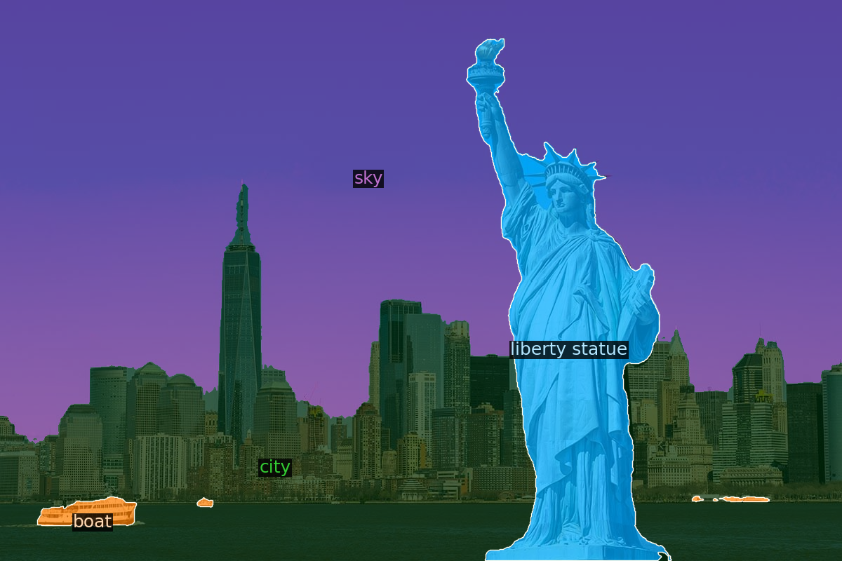
Figure 1: Self-Guided Open-Vocabulary Semantic Segmentation. Our method is capable of determining and segmenting relevant open vocabulary class names automatically.

Given the scale, training VLMs comes at a extremely high computational cost. Because of this, it is common in literature to build upon pre-trained VLMs such as CLIP [22] or BLIP [15]. However, applying these VLMs on per-pixel tasks is non-trivial, as they are trained on full images and lack the ability to directly reason over local regions in the image. Previous attempts have employed a two-stage approach where masked regions are fed to the VLMs to produce CLIP embeddings, which are subsequently correlated with text encodings of text prompts to perform classification [33, 16, 7]. Other works directly align per-pixel embeddings with text embeddings retrieved from CLIP [14] based on text prompts provided by the user at test time. While training these models, the text prompts usually correspond to the ground truth class names of the dataset in question. In this paper, we take the capabilities of VLMs one step further and tackle a more challenging task in which the relevant class names are automatically generated. We enable self-guided open-vocabulary semantic segmentation, in which the goal is to produce accurate object segmentation and their pixel-level classifications for any class without the need for textual input from the user or predefined class names.

To tackle this task, we introduce a Self-Guided Semantic Segmentation (Self-SEG) framework. Our framework can adapt to any pre-trained segmentation backbone limited by the need for textual input describing the class names to be potentially segmented. In order to automate this, we propose BLIP-Cluster-Caption (BCC) which consists of four simple steps: 1) obtain local BLIP embeddings at different image scales; 2) cluster local BLIP embeddings to identify and separate meaningful semantic areas in the image; 3) caption each clustered embedding and extract nouns from the caption; and 4) pass the resulting nouns to a pre-trained segmentation backbone as class names, thereby essentially creating a self-guided network without any additional supervised training.

Experimental evaluations on Pascal VOC [9], ADE20K [37] and CityScapes [6] showcase the effectiveness of our framework. Self-SEG achieves state-of-the-art results on self-guided open-vocabulary semantic segmentation and competitive results with methods where class names are given. It is capable of predicting crisp segmentation masks without having any information a priori about which objects to segment (see Fig. 1). For effective evaluation on public datasets, we furthermore propose an LLM-based Open-Vocabulary Evaluator (LOVE), tasked with mapping open-vocabulary predictions to class names in the dataset using a Large Language Model (LLM). All code will be publicly released to ensure reproducibility and to facilitate further research.

In summary, our contributions are as follows: 1) we introduce Self-SEG, a novel framework to automatically determine and segment relevant classes in an image; 2) we propose BLIP-Cluster-Caption, a novel image captioning method capable of generating local and semantically meaningful descriptions from the image obtained from clustered BLIP embeddings; and 3) we propose LOVE, a novel evaluation method for open-vocabulary semantic segmentation which utilizes an LLM.

Through qualitative and quantitative analyses, we demonstrate the effectiveness of our Self-Guided Semantic Segmentation framework on multiple public datasets.

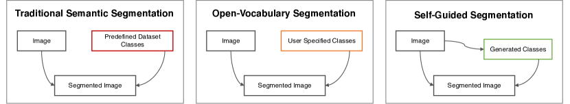
Figure 2: Different Semantic Segmentation Tasks in Comparison. Left: In traditional semantic segmentation, an image is segmented into fixed, predefined dataset classes used during annotation. Middle: In open-vocabulary segmentation, the user specifies which object categories (from the open vocabulary) need to be segmented. Right: In self-guided segmentation, relevant object categories are generated from the image automatically, enabling a true open-vocabulary understanding of scenes without a human in the loop.

2 Related Work

Open-Vocabulary Segmentation (OVS). OVS refers to the challenging task of segmenting images based on a list of arbitrary text queries. Contrary to traditional segmentation methods, OVS is not limited to a predefined set of classes. The field of OVS has seen significant advancements through different approaches. Approaching OVS as a zero-shot task, pioneering work by ZS3Net [1] and SPNet [29] trained custom modules that translate between visual and linguistic embedding spaces and segment by comparing word vectors and local image features. These methods attempt to learn the challenging connection between two very different and independent latent spaces. Consequently, the field of OVS has seen the introduction of methods incorporating Vision-Language Models (VLMs). VLMs pre-train a visual feature encoder with a textual feature encoder on large amounts of image-text pairs, enabling image and text representations to reside in the same feature space. One of such VLMs, Contrastive Language-Image Pre-training (CLIP) [22], has triggered a wave of segmentation approaches that harness pretrained CLIP embeddings for OVS. LSeg [14] proposed a Dense Prediction Transformer to generate per-pixel CLIP embeddings, which are then compared to class embeddings derived from ground-truth segments. More popularly, two-stage approaches such as OpenSeg [10], OPSNet [3], OVSeg [16], ZSSeg[33] and POMP [24] first obtain class-agnostic masks and use CLIP to classify each mask afterwards. Other works, including MaskCLIP [7], FC-CLIP [36], and SAN [34], focus on utilizing intermediate representations from a frozen CLIP encoder. For example, MaskCLIP uses the token features of the ViT-based CLIP encoder and compares local features to class label embeddings instead of pooling them into a global CLIP embedding. The remarkable diversity in the usage of CLIP for OVS extends to works which leverage relationships between image semantics and class labels in CLIP space [5], use CLIP for binary mask prediction [35] or ensure segmentation consistency at different granularity levels using CLIP [28]. Several works have proposed to tackle OVS outside the realm of VLMs using text-to-image diffusion models [11, 32] or custom transformer networks [30, 17, 31, 38]. Most notably, X-Decoder introduces a generalized transformer model capable of performing various vision-language tasks using a single set of parameters. One common and important limitation of the described methods is the need for textual input as a form of guidance by the user. Our work presents a novel framework which enables self-guidance by automatically finding relevant object categories using localized image captioning. Closest and concurrent to our work is the Zero-Guidance Segmentation paradigm [25], in which clustered DINO [2] embeddings are combined with CLIP to achieve zero guidance by the user. Despite the similar setting, there are key differences. While we use the BLIP [15] model for both image clustering and caption generation, they design a complex pipeline consisting of image clustering with DINO, obtaining vision-language embeddings with CLIP and a custom attention-masking module, to then caption these with CLIP-guided GPT-2. This requires converting between three different latent representations throughout the process. In contrast, we achieve superior segmentation quality by enabling self-guidance using any OVS model.

Image Captioning with Image-Text Embeddings. Image Captioning is the task of describing the content of an image using natural language. A number of approaches have been proposed for the task, including ones utilizing VLMs. Approaches such as CLIP-Cap [20] and CLIP-S [4] utilize CLIP embeddings to guide text generation. Other approaches rely on BLIP [15], a VLM in which the task of decoding text from image features was one of the tasks of the pretraining process. This enables BLIP to perform image captioning without additional components. Furthermore, the text decoder is guided by local patch embeddings in a way that enables local captioning based on a specific area. This unique capability, discovered during the development of our method, emerges organically in BLIP despite being trained solely with image-level captions.

Visual Phrase Grounding. Visual phrase grounding aims to connect different entities mentioned in a caption to corresponding image regions [26]. This task resembles OVS, as it aims to find correspondences between text and image regions. However, predicted areas do not have to precisely outline object boundaries and can be overlapping. Visual grounding has been approached in a self-guided manner, in which heatmaps of regions of the image are generated from image-level CLIP embeddings, which are then captioned by the BLIP encoder [27]. One disadvantage of this approach is that the region determined by CLIP can indicate multiple objects at once, hence multiple objects are captioned for that region, preventing pixel-level class-specific predictions. In our work, BLIP is used both as an encoder and decoder, which enables for category-specific regions and captioning.

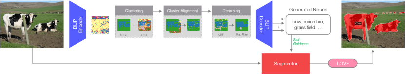
Figure 3: Method Overview. BLIP encodings are clustered, aligned and denoised before being decoded into nouns. Generated nouns serve as self-guidance to an OVS model, which outputs the final mask. During evaluation, we process the output mask with our custom evaluator LOVE, which maps predicted nouns to dataset class names.

3 Method

The aim of this paper is to perform open vocabulary semantic segmentation without training, finetuning or textual input. To this end, we propose to identify relevant object categories in the image by captioning local regions in the image at different scales (Sect. 3.1), filtering the generated captions into meaningful semantic descriptions (Sect. 3.2) and using these as self-guidance for a segmentor (Sect. 3.3). An overview of our method is depicted in Fig. 3.

3.1 Local Region Captioning

To identify relevant object categories in the image, we employ Bootstrapped Language Image Pretraining (BLIP) [15]. BLIP is a powerful VLM able to perform accurate and detailed image captioning. The BLIP image encoder is designed as a Vision Transformer [8], dividing the image into patches and encoding them into embeddings in which image-text representations reside. Subsequently, the set of embeddings is passed through transformer layers to capture contextual information across the image. Finally, all contextualized embeddings are passed to the decoder to generate text descriptions. Though effective in describing salient objects in the image, captioning models generally fail to describe all elements of a scene in a comprehensive way. This is likely due to the structure of training data, in which image descriptions mostly focus on salient foreground elements. This characteristic of VLM pre-training limits its direct application to downstream tasks such as open-vocabulary segmentation, in which many objects in the image go unnoticed. As a solution to this limitation, we seek to enable BLIP’s text decoder to consider all encoded areas in the image. Therefore, we propose to cluster the encoded BLIP features into semantically meaningful BLIP feature clusters, which are subsequently enhanced to capture the feature representation of real objects more effectively. Finally, each BLIP feature cluster is fed to the text decoder separately. This enables generating a description of each semantically meaningful area in the image, resulting in a more complete description of the image overall.

Clustering. By default, BLIP expects an RGB image $\mathbf{X}_{D}\in\mathbb{R}^{384\times 384\times 3}$. We additionally process the image at a larger resolution $\mathbf{X}_{L}\in\mathbb{R}^{512\times 512\times 3}$, as common datasets often have images with higher resolution. The multi-resolution set of images $\mathbf{X}=\{\mathbf{X}_{D},\mathbf{X}_{L}\}$ is fed to the BLIP encoder to obtain the set of BLIP patch embeddings $\mathbf{B}$ at the two resolutions:

$$\mathbf{P}^{\mathbf{X}_{D}} =\left\{\mathbf{X}^{D}_{ij}\,|\,\mathbf{X}^{D}_{ij}\in\mathbb{R}^{16\times 16\times 3},1\leq i,j\leq 24\right\}$$ (1)

$$\mathbf{P}^{\mathbf{X}_{L}} =\left\{\mathbf{X}^{L}_{ij}\,|\,\mathbf{X}^{L}_{ij}\in\mathbb{R}^{16\times 16\times 3},1\leq i,j\leq 32\right\}$$ (2)

$$\mathbf{B}^{\mathbf{X}_{D}} =T\big{(}f_{\text{MLP}}(\mathbf{P}^{\mathbf{X}_{D}})\big{)}\quad\textbf{B}^{\mathbf{X}_{L}}=T\big{(}f_{\text{MLP}}(\mathbf{P}^{\mathbf{X}_{L}})\big{)}$$ (3)

$$\hat{\mathbf{B}}^{\mathbf{X}_{R}}_{i} =\mathbf{B}^{\mathbf{X}_{R}}_{i}\oplus\mathbf{z}^{\mathbf{X}_{R}}_{i},\quad\forall i\in\{1,2,\ldots,N\}$$ (4)

where $\textbf{P}^{\textbf{X}_{D}}\in\mathbb{R}^{576\times 16\times 16\times 3}$ and $\textbf{P}^{\textbf{X}_{L}}\in\mathbb{R}^{1024\times 16\times 16\times 3}$ denote the set of patches for the default and large resolutions $D$ and $L$ respectively, $f_{\text{MLP}}(\cdot)$ represents a shared fully connected Multi-Layer Perceptron (MLP) and $T$ is a Transformer encoder, consisting of $L$ alternating layers of Multi-Head Self-Attention (MHA) and an MLP:

$$T_{l}(X) =\textsc{LayerNorm}\big{(}X+\textsc{MHA}(X,X,X)\big{)}$$ (5)

$$T^{\prime}_{l}(X) =\textsc{LayerNorm}\big{(}T_{l}(X)+f_{\text{MLP}}(T_{l}(X))\big{)}$$ (6)

$$T(X) =T^{\prime}_{L}\circ T^{\prime}_{L-1}\circ\ldots\circ T^{\prime}_{1}(X).$$ (7)

In Eq. (4), we additionally concatenate a sin-cos positional embedding $\mathbf{z}_{i}\in\mathbb{R}^{256}$ to each patch $i$ to encode spatial information, where $N$ is the total number of patches for each resolution $R$. Next, we cluster the patches in $\hat{\mathbf{B}}$ for each resolution $R$ using $k$-means clustering [19]:

$$C^{R}_{k}= \underset{C}{\operatorname{argmin}}\sum_{i=1}^{N}\min_{\mu_{j}\in C}\|\hat{\mathbf{B}}^{\mathbf{X}_{R}}_{i}-\mu_{j}\|^{2}$$ (8)

where $C_{k}$ is the set of $k$ clusters and $\mu_{i}$ are the cluster centroids. Running the clustering procedure with two unique values for $k$ on two different image resolutions results in four different cluster assignments.

Cross-clustering Consistency.

Each run of $k$-means clustering labels its clusters independently from others, yielding a correspondence issue between clusters across runs. To resolve this, we relabel the cluster indices to a common reference frame with the following steps:

1. We pick the set of clusters with the most clusters after $k$-means as a reference set $S$. This is not necessarily the set with highest initial k, because some clusters can become empty during the $k$-means iterations. The reference set determines the indices used for all other sets of clusters $\mathcal{C}$, each with its number of clusters denoted by $|C_{i}|$:

   $$S=\underset{C_{i}\in\mathcal{C}}{\mathrm{argmax}}\,|C_{i}|$$ (9)

2. Sets of clusters are aligned to the reference set using Hungarian matching [13]. Given the reference set $S$ and another set of clusters $C$, we calculate pairwise IoU (Intersection over Union) between the clusters from $R$ and $C$. Then, each cluster from $C$ is assigned a new index, matching the cluster with the highest IoU from $S$:

   $$\text{For each cluster }c_{j}\in C,\quad j\in\{1,\ldots,|C|\}:$$

   $$\text{Assign }c_{j}\text{ to }r_{i}\text{ where }i=\!\underset{i\in\{1,\ldots,|S|\}}{\mathrm{argmax}}\,\text{IoU}(c_{j},r_{i})$$ (10)

3. With the labeled sets of clusters, we assign a probability distribution over the clusters to each image patch. For a given patch $p$, let $L(p)=\{L_{1}(p),L_{2}(p),\ldots,L_{m}(p)\}$ be the set of labels assigned to $p$ by the $m$ different sets of clusters. The probability $P(n|p)$ of $p$ being assigned to a particular cluster $n$ is defined as the relative frequency of $n$ among labels $L(p)$:

   $$P(n|p)=\frac{\sum_{i=1}^{m}\mathbbm{1}}{m},\text{\small with }\mathbbm{1}=\begin{cases}1,&\text{\small if }L_{i}(p)=n\\ 0,&\text{\small else}\end{cases}$$ (11)

The predictions of a single $k$-means predictor tend to contain high levels of noise, likely due to the high dimensionality of the embeddings. Our method can be seen as an ensemble, reducing the variance present in each individual predictor. The areas that are consistently clustered together by various predictors are likely to be semantically connected. In addition, our method enables for a flexible number of output clusters. Some of the initial clusters can disappear if they are not well-supported by multiple predictors. This property is highly desired due to the variety of input images and the number of objects in them.

Cluster Denoising. To further improve the locality and semantic meaningfulness of clustered feature representations, we apply a Conditional Random Field (CRF) [12] and majority filter. CRF is a discriminative statistical method that is used to denoise predictions based on local interactions between them. In our case, the predictions are a 2D grid of cluster assignment probabilities of the image patches. The CRF implementation we use is specifically tailored for refining 2D segmentation maps. It uses a mean field approximation with a convolutional approach to iteratively adjust the probability distributions of each image patch’s cluster indices. Key to this process is the use of a Gaussian filter in the pairwise potentials, which ensures spatial smoothness and consistency in the segmentation.

As shown in Fig. 3, the application of the CRF yields clusters which are cleaner and more cohesive than the original aligned $k$-means result. To address any remaining noise in the resulting clusters, we apply a neighborhood majority filter as a final step. For each image patch, we consider the set of patches $\mathcal{N}(i,j)$ in its square neighborhood: $\mathcal{N}(i,j)=\{(i+\delta_{i},j+\delta_{j})\,|\,\delta_{i},\delta_{j}\in\{-1,0,1\}\}$. We calculate the mode value from the cluster indices in that neighborhood and assign it as the new index of the central patch:

$$\text{mode}\big{(}\mathcal{N}(i,j)\big{)}=\underset{k\in K}{\mathrm{argmax}}\sum_{m\in\mathcal{N}(i,j)}\mathbbm{1}_{\text{index}(m)=k}$$ (12)

This step is applied recursively until convergence or 8 times at most.

Caption Generation. The next step involves turning clustered, denoised and enhanced BLIP embeddings into text. The BLIP text decoder is a Transformer architecture capable of processing unordered sets of embeddings of arbitrary size. We leverage this feature and feed flattened subsets of patch embeddings, each corresponding to a cluster, to the BLIP text decoder. Spatial information is preserved due to the presence of positional embeddings added in the clustering step. With this technique, our method essentially iterates over semantic categories captured by clusters and represented by BLIP embeddings. To the best of our knowledge, we are the first to use the text decoder in this manner, enabling local captioning for which it was never specifically trained. The caption generation is stochastic, with different object namings appearing in the captions depending on random initialization. To obtain a rich, unbiased and diverse set of object names, we regenerate captions with each embedding multiple times in caption generation cycles.

3.2 Caption Filtering

The captions generated by the BLIP text decoder are sentences in natural language. For our task, we are only interested in the class names present in each sentence. To obtain these, we filter the sentence down to relevant class names using noun extraction. Captions are parsed using the spaCy model to provide a part-of-speech label for each word in the caption. Words labeled as nouns are kept and converted into their singular form through lemmatization. We collect all nouns generated by different clusters and cycles into one noun set and remove any duplicates, as well as nouns which do not appear in the WordNet dictionary.

3.3 Self-Guidance

The output of the clustered BLIP embeddings (see Sect. 3.1) is a 32x32 grid with cluster index assignments. Each element of the grid corresponds to an image patch from the original image, which enables us to create segmentation masks - defined as a union of areas covered by image patches with the same index - essentially for free. For example, Fig. 3 shows the clustered output as a 2-dimensional mask, which succeed in masking relevant objects to a certain extent. However, the segmentation outputs are constrained to a 32x32 resolution of the BLIP encoder. Upsampling yields unsatisfactory results, since objects appear oversegmented and boundaries remain unsharp. Another challenge is to associate each mask with one class name. In this cluster representation, masked areas are described with sentences rather than single nouns. When such a sentence contains multiple nouns, it is not trivial which noun to select as the predicted class name for that mask. To perform effective and accurate open-vocabulary semantic segmentation, we leverage Blip-Cluster-Caption’s strength in generating an elaborate set of relevant class names and use this as guidance for a pre-trained OVS model capable of producing high-resolution outputs. BLIP-Cluster-Caption is model-agnostic, therefore any kind of OVS model that expects an image and a set of class labels can be combined with our method. We focus on X-Decoder[38], which is a popular and well-performing OVS model.

3.4 Custom Open-Vocabulary Evaluator

As discussed in Sect. 2, previous works in OVS have mainly focused on a setting where the target class names are provided by the user. Hence, evaluation is possible by having access to the ground truth of those target class names during evaluation. However, in scenarios where the target class names are discovered rather than pre-specified, as in our framework, there may be a lack of direct alignment between the semantics of these categories and the classes used in the annotations. In zero-guidance segmentation [25], the authors have proposed to align class names based on the cosine-similarity in the latent space of Sentence-BERT [23] or CLIP [22]. In our initial experiments, this yielded unsatisfactory results where even in obvious cases, the open-vocabulary classes were linked to the incorrect class. Relations between two class names can be complex, such as synonymity, hyponymy, hypernymy, meronymy or holonymy, which exceed the capabilities of a cosine-similarity criterium in the respective latent spaces. As a possible solution, we propose an LLM-based Open-Vocabulary Evaluator (LOVE). Specifically, we employ the Llama 2 7B Large Language model with the task of mapping predicted open-vocabulary categories to target categories in the dataset. First, Self-SEG returns a segmentation mask with classes from an open vocabulary generated by Blip-Cluster-Caption. Second, LOVE collects all unique predicted open-vocabulary categories in the output and builds a mapper from each predicted category to the most relevant target category. Thirdly, all values in the segmentation mask belonging to each class are updated respectively according to the mapper. Finally, the mIoU is computed with the updated segmentation mask. Pseudocode and prompts for LOVE are provided in App. A.

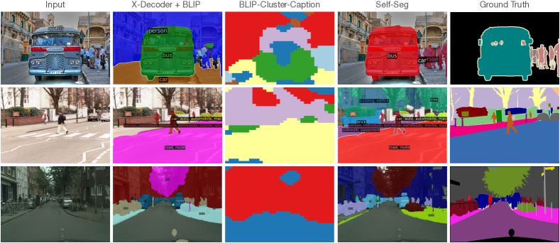
Figure 4: Segmentation Using VLMs. Example outputs from VOC (top), ADE20K (middle), CityScapes (bottom) obtained with different configurations of our self-guidance framework, from which Self-SEG performs most accurately with automatically detected class names.

4 Experiments

4.1 Experimental Setup

We evaluate our method on three popular semantic segmentation validation datasets: Pascal VOC [9], ADE20K [37] and CityScapes [6] with 20, 847 and 20 classes respectively. These datasets cover a wide range of difficulty and class diversity. For example, ADE20K is challenging due to a large variety of classes with many of them appearing only a few times in the whole dataset. We list dataset statistics in Tab. 3. For qualitative comparison with previous works, we use mean Intersection over Union (mIoU) as the main evaluation metric. As mentioned in Sec. 3.4, class predictions in the segmentation mask are mapped using LOVE before the mIoU is computed. To study the class-agnostic segmentation performance of different VLMs, we use class-agnostic mean Intersection over Union (cmIoU). The computation of cmIoU involves the following steps. First, pairwise IoU values, denoted as $\text{IoU}(g_{i},p_{j})$ are calculated between all ground-truth segments $g_{i}$ and predicted segments $p_{j}$ from a given image. Each $g_{i}$ segment is matched with the predicted segment $p_{\text{max}_{i}}$ that yields the highest IoU value: $p_{\text{max}_{i}}=\arg\max_{j}\text{IoU}(g_{i},p_{j})$. The cmIoU is then determined by calculating the arithmetic mean of these highest IoU values across the dataset, which can be formulated as $\text{cmIoU}=\frac{1}{N}\sum_{i=1}^{N}\text{IoU}_{\text{max}_{i}}$ where $N$ is the total number of ground-truth segments in the dataset.

In the Self-SEG model used for our experiments, we use the BLIP model built with ViT-Large backbone and finetuned for image captioning on the COCO dataset in combination with the Focal-T variant of X-Decoder. For both models, we use publicly available pretrained weights and do not perform any additional finetuning. Parameter tuning is performed for the clustering and captioning modules. Parameters of the clustering include image scales encoded by BLIP ($384\times 384$ and $512\times 512$), the $k$ values of $k$-means clustering (2 and 8), the parameters of Gaussian smoothing in the CRF (smoothness weight of 6 and smoothness $\theta$ of 0.8), the number of iterations of majority filtering (8) and the feature dimension size of the positional embeddings (256). As for text generation, we opted for nucleus sampling with a minimum length of 4 tokens and maximum of 25, top P value of 1 and repetition penalty of 100 to ensure as many unique nouns as possible. The aforementioned parameters were determined using Bayesian optimization on the Pascal VOC with the goal of maximizing the mIoU.

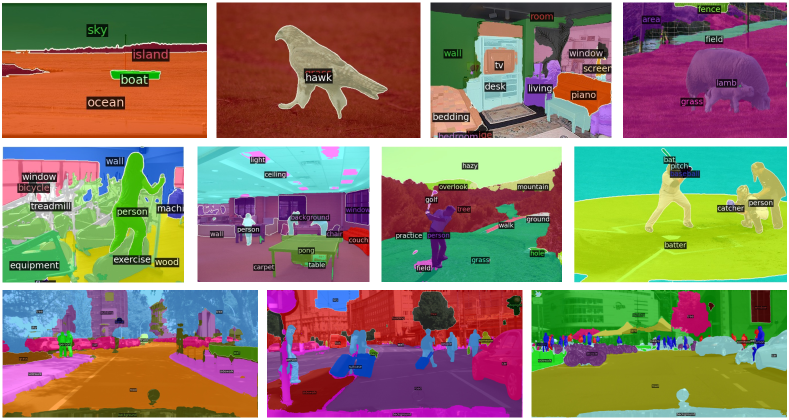
Figure 5: Qualitative Results. Self-SEG shows remarkable capability to identify open vocabulary class names and segment them accurately across different datasets (top, middle, bottom row are from VOC, ADE20K and CityScapes respectively).

4.2 Ablations

To investigate the performance of different configurations of our framework, we present two ablation studies. The first ablation study investigates different methods of using a VLM to obtain segmentation masks. In the second one, we examine the effect of different amounts of captioning cycles.

Segmentation with Vision Language Models. A VLM can be leveraged in different ways to obtain segmentation masks. In this ablation study, we compare three methods: 1) noun-filtered captions of a plain BLIP encoder/decoder as textual guidance for X-Decoder, which then produces the final segmentation; 2) BLIP cluster embeddings from our Blip-Cluster-Caption approach used as segmentation masks (see Sect. 3.3); and 3) Self-SEG in which textual guidance is achieved through Blip-Cluster-Caption and then provided to X-Decoder. Due to the difficulty with establishing correspondence between BCC clusters and ground-truth labels, we evaluate using cmIoU. Quantitative and qualitative results are reported in Tab. 1 and Fig. 4 respectively. On all three datasets, Self-SEG performs most effectively. Comparing X-Decoder + BLIP to Self-SEG qualitatively, one can observe that the former suffers from false positives and false negatives simultaneously, which in turn serves as an explanation for the performance gap in cmIoU. For example, in Pascal VOC, it incorrectly masks the area around the bus at the cost of segmenting people. In ADE20K, it ignores large parts of the area which could appear to BLIP as insignificant. In our framework, the BLIP-Cluster-Caption ensures that smaller, less salient objects are effectively captioned. As expected, intermediate masks of BLIP-Cluster-Caption do not segment objects sufficiently accurate due to the low resolution of the embedding space. Interestingly, it is still capable of segmenting global areas linked to certain objects in Pascal VOC and ADE20K, while failing completely for CityScapes, likely due to the higher instance count.

Approach	VOC [9]	ADE20K [37]	CityScapes [6]
X-Decoder [38] + BLIP [15]	38.0	26.7	29.2
Blip-Cluster-Caption	16.3	11.3	0.85
Self-SEG	41.9	29.2	35.8

Table 1: Ablations on Segmentation with VLMs. The cmIoU values obtained by different variants of our method. Self-SEG, which combines BCC with X-Decoder segmentation, achieves the best performance on all three datasets.

Captioning Cycles. One important feature of Self-SEG is that it can repeat the process of captioning from BLIP clusters in order to obtain a more elaborate set of nouns. This is particularly useful in situations where objects are initially missed or captioned with a suboptimal semantic description. We analyze the effect of captioning once or repeating the process 5, 10, 15, 20 or 25 times while measuring the mIoU performance. Our results, shown in Tab. 3, indicate that the optimal number of captioning cycles strongly depends on the dataset used. In particular, this number increases with the average amount of instances and unique classes per image (indicated with $\overline{I}$ and $\overline{C}$ in Tab. 3 respectively). For Pascal VOC, a dataset which contains fewer instances and unique classes per image, a single cycle is sufficient for Blip-Cluster-Caption to determine the relevant class names. It should be noted, however, that the average number of instances and classes per image are statistics obtained from the annotations of the dataset. In Pascal VOC, many objects that exist in the images are not annotated and are therefore considered background when evaluated. Hence, the actual optimal number of captioning cycles might be higher. In contrast to Pascal VOC, ADE20K, which contains on average 16 more instances and 7 unique classes per image, requires ten captioning cycles to obtain optimal performance. In the case of CityScapes, images are more complex with 34.3 instances and 17 unique classes on average. Here, twenty cycles of Blip-Cluster-Caption enable the model to obtain an mIoU score of 41.1, whereas Self-SEG would obtain 27.4 mIoU if it had used a single cycle. These outcomes indicate that increasing the number of captioning cycles with higher counts of instances and unique classes per image enable identifying more relevant objects, which in turn benefits the final segmentation output.

Method	Auto-Classes	VOC [9]	ADE20K [37]	CityScapes [6]
ZSSeg [33]	✗	83.5	7.0	34.5
FC-CLIP [36]	✗	95.4	14.8	56.2
X-Decoder [38]	✗	96.2	6.4	50.8
OpenSeg [10]	✗	72.2	8.8	-
ODISE [32]	✗	82.7	11.0	-
OVSeg [16]	✗	94.5	9.0	-
SAN [34]	✗	94.6	12.4	-
CatSeg [5]	✗	97.2	13.3	-
LSeg [14]	✗	47.4	-	-
OVSegmentor [31]	✗	53.8	-	-
SimSeg [35]	✗	57.4	-	-
OVDiff [11]	✗	69.0	-	-
ZeroSeg [25]	✓	20.1	-	-
Self-SEG (Ours)	✓	41.6	6.4	41.1

Table 2: Quantitative Results. Self-SEG performs competitive with existing OVS methods which require class names, while achieving superior performance on the zero label setting.

4.3 Quantitative Analysis

We compare our method against existing OVS methods that require class names to be given, as well as with Zero-Guidance Segmentation (referred to as ZeroSeg [25]). Tab. 2 shows the results. Without any specification of class names, Self-SEG achieves 43%, 43% and 73% of the best performing OVS methods on Pascal VOC, ADE20K and CityScapes respectively. In the ADE20K dataset, Self-SEG is able to remarkably match the performance of X-Decoder [38] without any access to the ground truth class names, while on CityScapes it even outperforms ZSSeg [33] by 6.6 mIoU. It is noteworthy that on CityScapes, our method achieves 81% of X-Decoder’s original performance with given class names. Comparing to ZeroSeg, Self-SEG achieves superior performance on Pascal VOC (41.6 over 20.1 mIoU). Furthermore, we set a new state-of-the-art on ADE20K and CityScapes under the auto-class generation task setting. This outcome underscores the efficacy of our method in dealing with complex scenes that have an open-vocabulary nature, such as ADE20K with its large number of rare classes. While other models have to decide between 847 possibilities, Self-SEG suggests a smaller yet relevant set of class names. Our method deals well with high number of instances and can successfully identify various non-salient objects. A comparison with the findings from Tab. 3 reveals that while Blip-Cluster-Caption struggles with providing high-quality masks, it is able to identify the relevant class names, which can subsequently be segmented accurately using an OVS model. This demonstrates that the integration of Blip-Cluster-Caption and OVS harnesses the strengths of both, leading to enhanced self-guided segmentation performance.

		Number of Captioning Cycles
Dataset		$\overline{I}$	$\overline{C}$	$C$	1	5	10	15	20	25
Pascal VOC [9]		3.5	3.5	20	41.6	37.9	37.4	35.6	35.1	35.6
ADE20K [37]		19.5	10.5	847	5.1	5.9	6.4	5.9	6.1	6.0
CityScapes [6]		34.3	17	20	27.4	35.9	39.7	40.2	41.1	41.0

Table 3: Ablations on Captioning Cycles. The optimal number of captioning cycles strongly depends on the dataset. Datasets with more instances ($\overline{I}$) and classes on average ($\overline{C}$) benefit from multiple cycles, while captioning once for few instances suffices.

4.4 Qualitative Analysis

Fig. 5 and App. B show qualitative results on the three datasets. Self-SEG is able to exhaustively identify relevant object classes present in the image while segmenting them accurately. Its ability to caption with specific class names such as hawk or treadmill showcases the model’s capabilities for OVS in the wild.

5 Conclusion

In this work we introduced Self-SEG, a novel method which leverages a vision-language model to automatically identify relevant object categories and segment them. In addition, we propose LOVE, a new evaluation method which employs an LLM to map from generated class names to ground-truth labels. Our method performs remarkably, achieving state-of-the-art performance on the zero label setting, while being competitive with open-vocabulary models which require ground-truth labels.

Acknowledgements. This work was supported by TomTom, the University of Amsterdam and the allowance of Top consortia for Knowledge and Innovation (TKIs) from the Netherlands Ministry of Economic Affairs and Climate Policy.

Appendices

Appendix A LLM-based Open-Vocabulary Evaluator

This appendix provides more insight into the pseudocode and text prompts of the LLM Mapper which maps open vocabulary classes to classes in the annotations of the dataset. The LLM Mapper is a key component of our LLM-based Open Vocabulary Evaluation Metric (LOVE) and enables the evaluation of predicted open vocabulary classes.

Pseudocode

The LLM Mapper is tasked with generating a mapping dictionary, which is used to change the predicted class index of each pixel to the corresponding class index in the dataset.

Algorithm 1 LLM Mapper

0:  nouns, dataset_vocabulary, llm_batch_size, prompt_template, LLM

  all_responses, map_dict, skipped $\leftarrow$ initialize()

  for batch in split(nouns, llm_batch_size) do

     dialogs $\leftarrow$ generateDialogs(batch, prompt_template)

     batch_responses $\leftarrow$ LLM(dialogs)

     store(all_responses, (batch_responses, batch))

  end for

  for (batch_response, batch) in all_responses do

     for (response, noun) in (batch_response, batch) do

        answer $\leftarrow$ parseResponse(response)

        common $\leftarrow$ intersect(answer, dataset_vocabulary)

        updateDict(map_dict, noun, common)

        updateSkipped(skipped, noun, common)

     end for

  end for

  for key in map_dict do

     if key is in vocabulary then

        map_dict[key] $\leftarrow$ key

     end if

     if key is in skipped then

        skipped $\leftarrow$ removeItem(skipped, key)

     end if

  end for

  for skipped_key in skipped do

     map_dict[skipped_key] $\leftarrow$ “background”

  end for

  return  map_dict

LLM Prompts

The generateDialogs() function in the LLM Mapper takes a prompt template as one of its inputs. This prompt template is dependent on the dataset and is used to generate dialogs to query the LLM with. For Pascal VOC and CityScapes, we explicitly specify the list of categories, while for ADE20K we rely on the LLM’s knowledge of the dataset. Since ADE20K has many classes, dialogues get very long otherwise. This causes the LLM to run into memory issues when queried with dialogues in batches. We specify the prompt templates for each dataset as follows:

Pascal VOC and CityScapes

To which class in the list <dataset> is
<name> exclusively most similar to? If
<name> is not similar to any class in
the list or if the term describes stuff
instead of things, answer with
’background’. Reply in single quotation
marks with the class name that is part
of the list <dataset> and do not link
it to any other class name which is not
part  of the given list or ’background’.

where <noun> is the noun to map to the vocabulary and <dataset> is the list of classes of Pascal VOC or CityScapes.

ADE20K

To which class in the ADE20K dataset
exclusively most similar to? If <noun>
is not similar to any class in ADE20K
or if the term describes stuff instead
of things, answer with ’background’.
Reply in single quotation marks with
the class name that is part of ADE20K
and do not link it to any other class
name which is not part of the given
list or ’background’.

Appendix B Qualitative Results

This appendix provides additional qualitative results of Self-Seg. With individual sample outputs of the model, we show and discuss both its abilities and limitations.

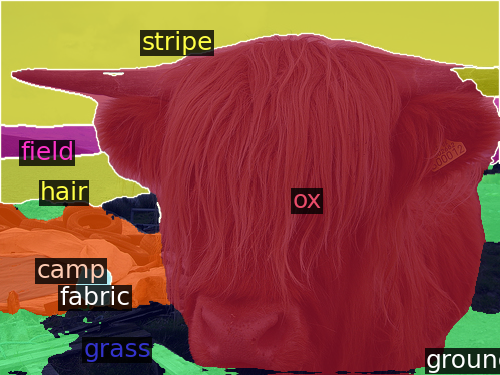
Figure 6: Self-Seg is able to accurately classify and segment classes not present in the dataset (here Pascal VOC), such as the ox.

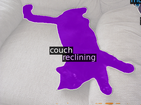
Figure 7: Interesting properties of objects are found with Blip-Cluster-Caption, such as reclining by the cat in this image.

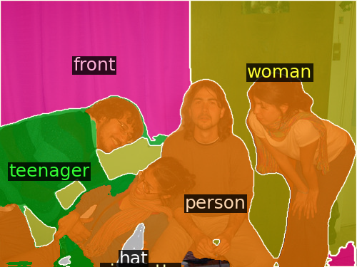
Figure 8: Generated nouns are occasionally hyponyms or hypernyms of each other, causing the classes to “compete” for the final segmentation. Future work could possibly address this by checking for such relations between nouns and correcting for them.

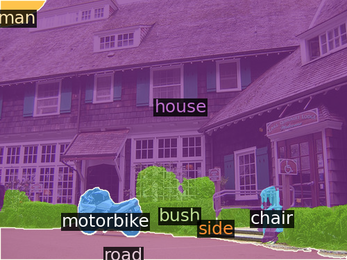
Figure 9: Self-guidance occasionally yields a false positive noun, here man, which is then incorrectly used and segmented by X-Decoder.

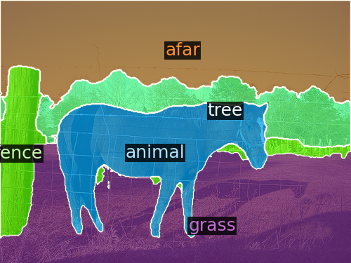
Figure 10: The generated nouns are occasionally too generic (here animal and afar). The predicted mask is accurate nevertheless.

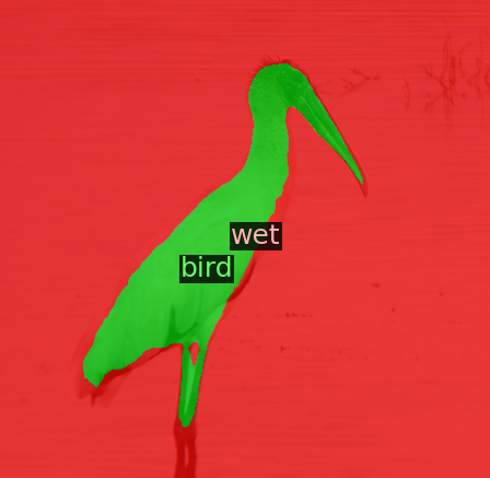
Figure 11: At times, an object or area is classified with one of its properties rather than the class name itself.

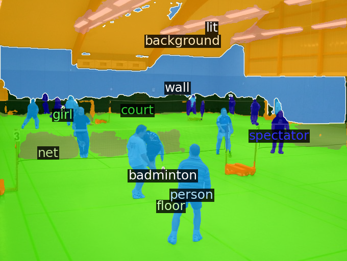
Figure 12: ADE20K has many classes, but badminton was not one of them. Despite being very small, it is still found and segmented.

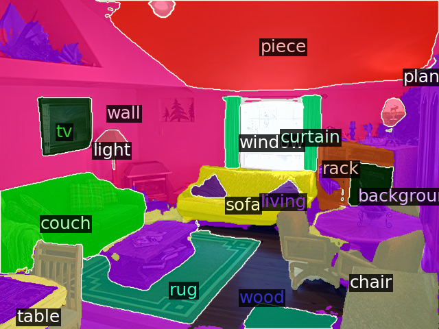
Figure 13: Even with many objects present, Self-Seg maintains good performance in spotting and segmenting the objects.

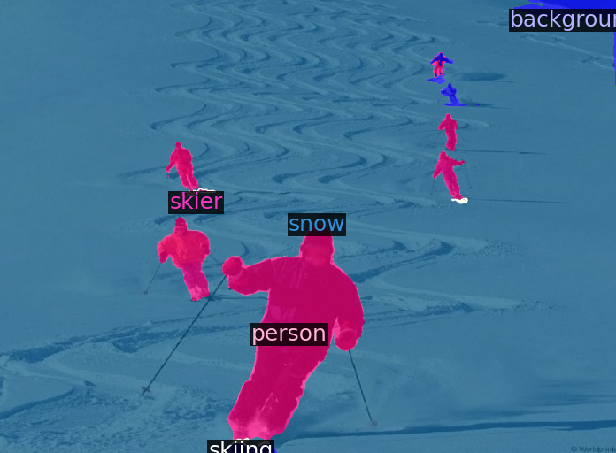
Figure 14: Self-Seg can identify and segment an activity present in the image. Shown here is skiing with a white segmentation mask around the feet of the skier.

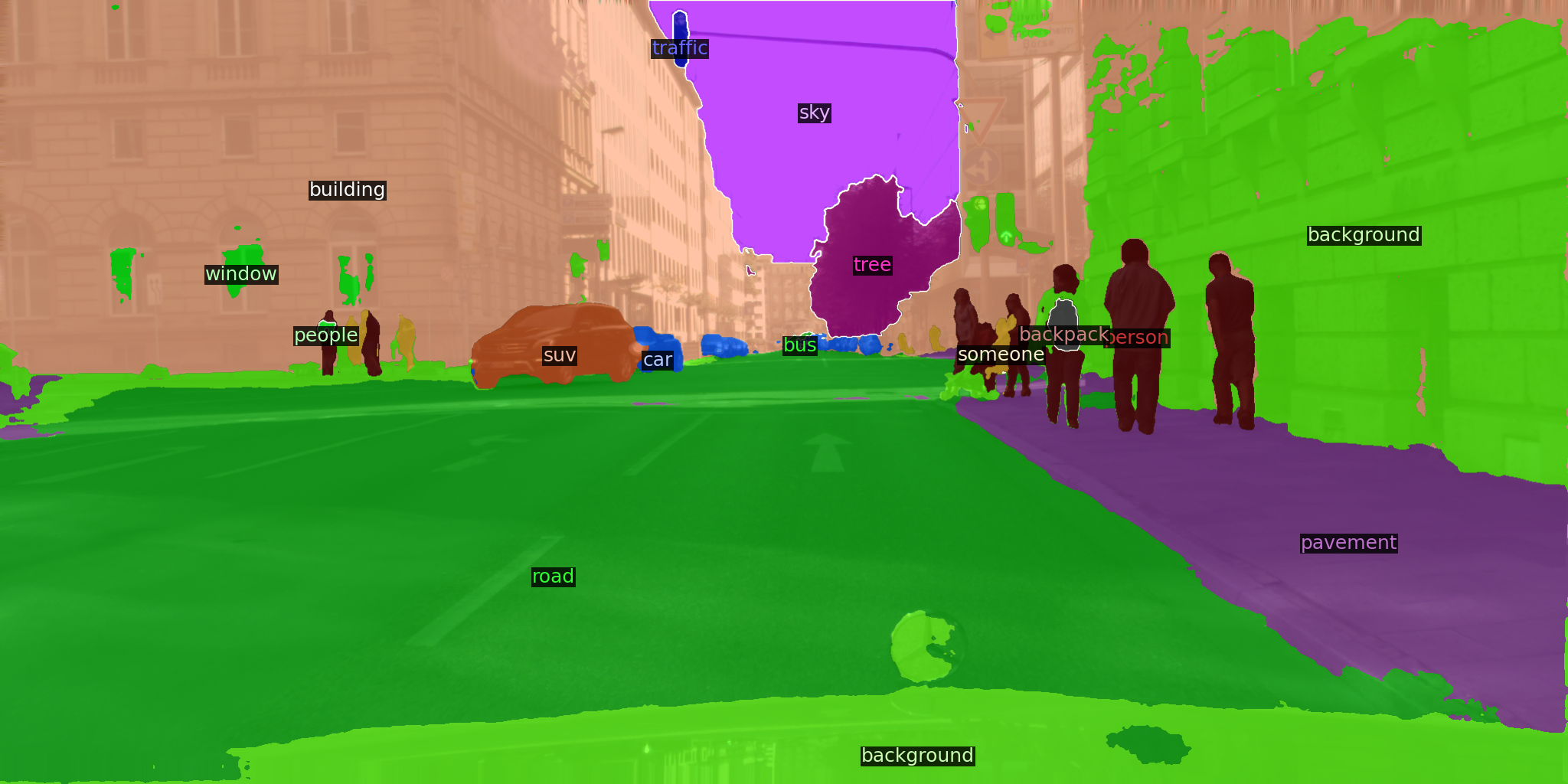
Figure 15: While in CityScapes all car types are considered equal, Self-Seg often provides more specific descriptions, such as the SUV in this image.

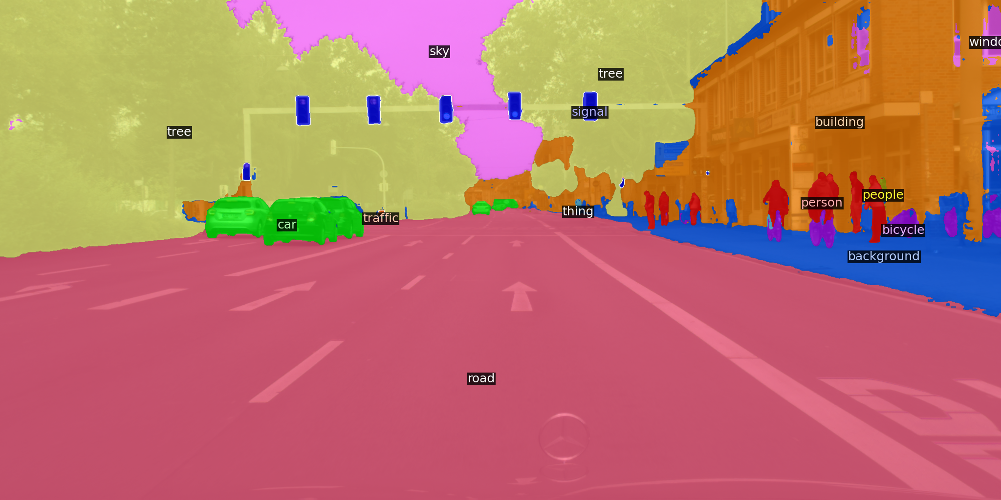
Figure 16: Self-Seg’s freedom in captioning the image with an open-vocabulary understanding of the world becomes evident in this example. Traffic lights in this scene are classified and segmented as signal.

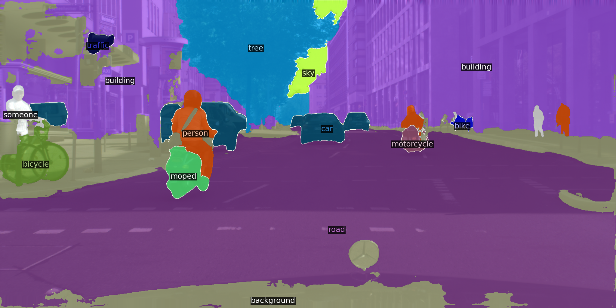
Figure 17: Despite the visual similarities between a moped and motorcycle, Self-Seg correctly considers both. It is able to distinguish between the two vehicles and segment them accurately. A supervised model would not be able to generalize to moped, as it is not one of the annotated classes in CityScapes.

References

- Bucher et al. [2019] Maxime Bucher, Tuan-Hung VU, Matthieu Cord, and Patrick Pérez. Zero-shot semantic segmentation. In NeurIPS, 2019.
- Caron et al. [2021] Mathilde Caron, Hugo Touvron, Ishan Misra, Hervé Jégou, Julien Mairal, Piotr Bojanowski, and Armand Joulin. Emerging properties in self-supervised vision transformers. In ICCV, 2021.
- Chen et al. [2023] Xi Chen, Shuang Li, Ser-Nam Lim, Antonio Torralba, and Hengshuang Zhao. Open-vocabulary panoptic segmentation with embedding modulation. In ICCV, 2023.
- Cho et al. [2023a] Jaemin Cho, Seunghyun Yoon, Ajinkya Kale, Franck Dernoncourt, Trung Bui, and Mohit Bansal. Fine-grained image captioning with clip reward. arXiv preprint arXiv:2205.13115, 2023a.
- Cho et al. [2023b] Seokju Cho, Heeseong Shin, Sunghwan Hong, Seungjun An, Seungjun Lee, Anurag Arnab, Paul Hongsuck Seo, and Seungryong Kim. Cat-seg: Cost aggregation for open-vocabulary semantic segmentation. arXiv preprint arXiv:2303.11797, 2023b.
- Cordts et al. [2016] Marius Cordts, Mohamed Omran, Sebastian Ramos, Timo Rehfeld, Markus Enzweiler, Rodrigo Benenson, Uwe Franke, Stefan Roth, and Bernt Schiele. The cityscapes dataset for semantic urban scene understanding. In CVPR, 2016.
- Dong et al. [2023] Xiaoyi Dong, Jianmin Bao, Yinglin Zheng, Ting Zhang, Dongdong Chen, Hao Yang, Ming Zeng, Weiming Zhang, Lu Yuan, Dong Chen, Fang Wen, and Nenghai Yu. Maskclip: Masked self-distillation advances contrastive language-image pretraining. arXiv preprint arXiv:2208.12262, 2023.
- Dosovitskiy et al. [2020] Alexey Dosovitskiy, Lucas Beyer, Alexander Kolesnikov, Dirk Weissenborn, Xiaohua Zhai, Thomas Unterthiner, Mostafa Dehghani, Matthias Minderer, Georg Heigold, Sylvain Gelly, et al. An image is worth 16x16 words: Transformers for image recognition at scale. arXiv preprint arXiv:2010.11929, 2020.
- Everingham et al. [2010] Mark Everingham, Luc Van Gool, Christopher K. I. Williams, John M. Winn, and Andrew Zisserman. The pascal visual object classes (voc) challenge. IJCV, 2010.
- Ghiasi et al. [2022] Golnaz Ghiasi, Xiuye Gu, Yin Cui, and Tsung-Yi Lin. Open-vocabulary image segmentation. ECCV, 2022.
- Karazija et al. [2023] Laurynas Karazija, Iro Laina, Andrea Vedaldi, and Christian Rupprecht. Diffusion Models for Zero-Shot Open-Vocabulary Segmentation. arXiv preprint arXiv:2306.09316, 2023.
- Krähenbühl and Koltun [2011] Philipp Krähenbühl and Vladlen Koltun. Efficient inference in fully connected crfs with gaussian edge potentials. Advances in neural information processing systems, 24, 2011.
- Kuhn [1955] Harold W Kuhn. The hungarian method for the assignment problem. Naval Research Logistics Quarterly, 2(1-2):83–97, 1955.
- Li et al. [2022a] Boyi Li, Kilian Q. Weinberger, Serge J. Belongie, Vladlen Koltun, and René Ranftl. Language-driven semantic segmentation. ICLR, 2022a.
- Li et al. [2022b] Junnan Li, Dongxu Li, Caiming Xiong, and Steven Hoi. Blip: Bootstrapping language-image pre-training for unified vision-language understanding and generation. In ICML, 2022b.
- Liang et al. [2023] Feng Liang, Bichen Wu, Xiaoliang Dai, Kunpeng Li, Yinan Zhao, Hang Zhang, Peizhao Zhang, Peter Vajda, and Diana Marculescu. Open-vocabulary semantic segmentation with mask-adapted clip. CVPR, 2023.
- Liu et al. [2022] Quande Liu, Youpeng Wen, Jianhua Han, Chunjing Xu, Hang Xu, and Xiaodan Liang. Open-world semantic segmentation via contrasting and clustering vision-language embedding. In ECCV, 2022.
- Ma et al. [2022] Chaofan Ma, Yuhuan Yang, Yanfeng Wang, Ya Zhang, and Weidi Xie. Open-vocabulary semantic segmentation with frozen vision-language models. In BMVC, 2022.
- MacQueen [1967] J MacQueen. Some methods for classification and analysis of multivariate observations. In Proceedings of the fifth Berkeley symposium on mathematical statistics and probability, pages 281–297, 1967.
- Mokady et al. [2021] Ron Mokady, Amir Hertz, and Amit H Bermano. Clipcap: Clip prefix for image captioning. arXiv preprint arXiv:2111.09734, 2021.
- Pandey et al. [2023] Prashant Pandey, Mustafa Chasmai, Monish Natarajan, and Brejesh Lall. A language-guided benchmark for weakly supervised open vocabulary semantic segmentation. arXiv preprint arXiv:2302.14163, 2023.
- Radford et al. [2021] Alec Radford, Jong Wook Kim, Chris Hallacy, Aditya Ramesh, Gabriel Goh, Sandhini Agarwal, Girish Sastry, Amanda Askell, Pamela Mishkin, Jack Clark, Gretchen Krueger, and Ilya Sutskever. Learning transferable visual models from natural language supervision. In ICML, 2021.
- Reimers and Gurevych [2019] Nils Reimers and Iryna Gurevych. Sentence-bert: Sentence embeddings using siamese bert-networks. EMNLP, 2019.
- Ren et al. [2023] Shuhuai Ren, Aston Zhang, Yi Zhu, Shuai Zhang, Shuai Zheng, Mu Li, Alex Smola, and Xu Sun. Prompt pre-training with twenty-thousand classes for open-vocabulary visual recognition. In NeurIPS, 2023.
- Rewatbowornwong et al. [2023] Pitchaporn Rewatbowornwong, Nattanat Chatthee, Ekapol Chuangsuwanich, and Supasorn Suwajanakorn. Zero-guidance segmentation using zero segment labels. In ICCV, 2023.
- Rohrbach et al. [2016] Anna Rohrbach, Marcus Rohrbach, Ronghang Hu, Trevor Darrell, and Bernt Schiele. Grounding of textual phrases in images by reconstruction. In ECCV, 2016.
- Shaharabany et al. [2022] Tal Shaharabany, Yoad Tewel, and Lior Wolf. What is where by looking: Weakly-supervised open-world phrase-grounding without text inputs. NeurIPS, 2022.
- Sun et al. [2023] Peize Sun, Shoufa Chen, Chenchen Zhu, Fanyi Xiao, Ping Luo, Saining Xie, and Zhicheng Yan. Going denser with open-vocabulary part segmentation. In ICCV, 2023.
- Xian et al. [2019] Yongqin Xian, Subhabrata Choudhury, Yang He, Bernt Schiele, and Zeynep Akata. Semantic projection network for zero- and few-label semantic segmentation. In CVPR, 2019.
- Xu et al. [2022a] Jiarui Xu, Shalini De Mello, Sifei Liu, Wonmin Byeon, Thomas Breuel, Jan Kautz, and Xiaolong Wang. Groupvit: Semantic segmentation emerges from text supervision. CVPR, 2022a.
- Xu et al. [2023a] Jilan Xu, Junlin Hou, Yuejie Zhang, Rui Feng, Yi Wang, Yu Qiao, and Weidi Xie. Learning open-vocabulary semantic segmentation models from natural language supervision. In CVPR, 2023a.
- Xu et al. [2023b] Jiarui Xu, Sifei Liu, Arash Vahdat, Wonmin Byeon, Xiaolong Wang, and Shalini De Mello. Open-Vocabulary Panoptic Segmentation with Text-to-Image Diffusion Models. ICCV, 2023b.
- Xu et al. [2022b] Mengde Xu, Zheng Zhang, Fangyun Wei, Yutong Lin, Yue Cao, Han Hu, , and Xiang Bai. A simple baseline for open vocabulary semantic segmentation with pre-trained vision-language model. ECCV, 2022b.
- Xu et al. [2023c] Mengde Xu, Zheng Zhang, Fangyun Wei, Han Hu, and Xiang Bai. Side adapter network for open-vocabulary semantic segmentation. In CVPR, 2023c.
- Yi et al. [2023] Muyang Yi, Quan Cui, Hao Wu, Cheng Yang, Osamu Yoshie, and Hongtao Lu. A simple framework for text-supervised semantic segmentation. In CVPR, 2023.
- Yu et al. [2023] Qihang Yu, Ju He, Xueqing Deng, Xiaohui Shen, and Liang-Chieh Chen. Convolutions die hard: Open-vocabulary segmentation with single frozen convolutional clip. In NeurIPS, 2023.
- Zhou et al. [2017] Bolei Zhou, Hang Zhao, Xavier Puig, Sanja Fidler, Adela Barriuso, and Antonio Torralba. Scene parsing through ade20k dataset. In CVPR, 2017.
- Zou et al. [2023] Xueyan Zou, Zi-Yi Dou, Jianwei Yang, Zhe Gan, Linjie Li, Chunyuan Li, Xiyang Dai, Harkirat Behl, Jianfeng Wang, Lu Yuan, Nanyun Peng, Lijuan Wang, Yong Jae Lee, and Jianfeng Gao. Generalized decoding for pixel, image, and language. CVPR, 2023.