Transient effects in quantum dots contacted via topological superconductor

Abstract

We investigate gradual development of the quasiparticle states in two quantum dots attached to opposite sides of the topological superconducting nanowire, hosting the boundary modes. Specifically, we explore the non-equilibrium cross-correlations transmitted between these quantum dots via the zero-energy Majorana modes. From the analytical and numerical results we reveal nonlocal features in the transient behavior of electron pairing, which subsequently cease while the hybrid structure evolves towards its asymptotic steady limit configuration. We estimate duration of these temporary nonlocal phenomena and inspect their possible manifestation in the quench-driven processes. Such dynamical effects might play an important role in braiding protocols of the topological and/or conventional superconducting quantum bits using nanoscopic hybrid structures.

I Introduction

Majorana quasiparticles localized at the edges of one-dimensional chains [1], propagating along the boundaries of two-dimensional topological superconductors [2] and confined on internal defects in $p$-wave bulk superconductors [3] have been recently the topic of intensive studies (see e.g. [4, 5, 6, 7, 8, 9] and references cites therein). Such research interests are motivated by the exotic character of Majorana modes and additionally stimulated by the perspectives for constructing the stable quantum bits (immune to external perturbations due to topological protection) and for performing quantum computations (by virtue of their non-Abelian character) [10]. Majorana quasiparticles, realized in various platforms, including the minimalistic Kitaev chain consisting of two quantum dots [11], do always emerge in pairs. To what extent, however, these spatially separated zero-energy modes are cross-correlated either statically (enabling teleportation phenomena [12, 13, 14, 15]) or dynamically is still a matter of controversy. Some theoretical studies have predicted that Majorana modes might exhibit their dynamical interdependence in the shot-noise [16, 17, 18, 19]. Yet, any evidence for such nonlocal cross-correlations is missing.

Another convenient platform for exploring the unique features of Majorana modes are hybrid structures, where single or multiple quantum dots are side-attached to topological superconductors [7]. Natural tendency of Majorana modes to be harbored at outskirts of the low-dimensional superconductors gives rise to their leakage onto the attached quantum dot(s) [20, 21, 22, 23, 24]. Such leakage has been indeed reported experimentally [25], stimulating further theoretical studies concerning the interplay of Majorana modes with the correlation-driven effects [26, 27, 28, 29, 30, 31, 32, 33, 34, 35, 36, 37]. Here we propose to consider similar hybrid structures, comprising two quantum dots interconnected through the topological superconductor, in order to search for possible signatures of their nonlocal feedback effects appearing under non-equilibrium conditions.

Specifically, we investigate the dynamical properties of our setup (displayed in Fig. 1) right after coupling its constituents. The system consists of two quantum dots hybridized with the topological superconducting nanowire, hosting the Majorana boundary modes. One of the quantum dots, QD₁, is embedded between the conventional superconductor (S) and normal (N) leads, enabling its quasiparticles to be probed by the Andreev (electron-to-hole scattering) spectroscopy. The second dot, QD₂, is flanked on the opposite side of the topological superconductor. These spatially distant quantum dots are communicated solely through the Majorana zero-energy modes of the topological superconductor. In what follows we inspect nonlocal phenomena, appearing in the transient dynamics of measurable observables.

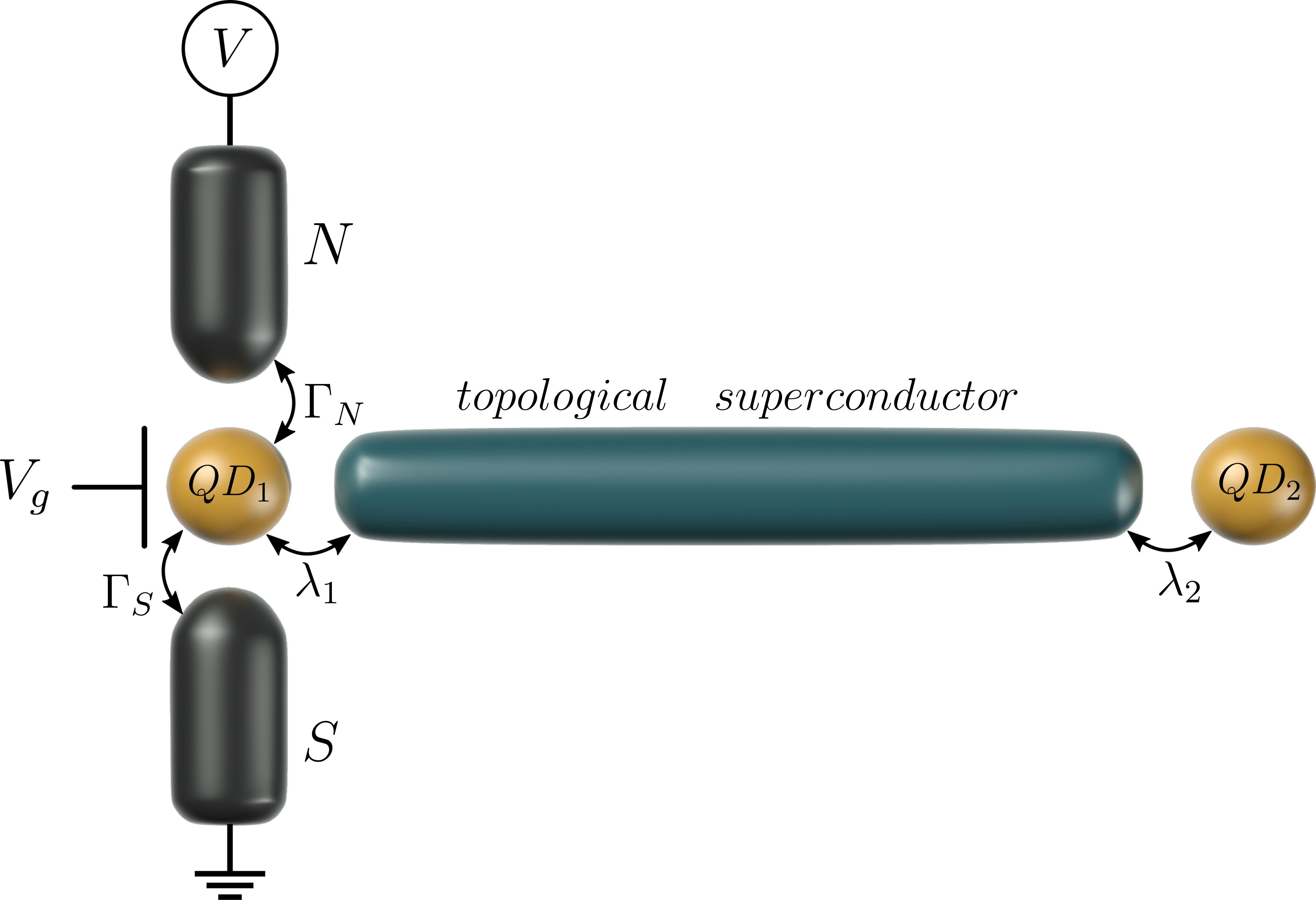
Figure 1: Schematic view of two quantum dots attached to opposite sides of the topological superconducting nanowire, hosting Majorana boundary modes. QD₁ is placed between the normal lead (N) and conventional superconductor (S), so that its emerging quasiparticles can be probed by the Andreev spectroscopy. The other quantum dot, QD₂, is floating.

It is important to note that the time-resolved studies of topological superconductors have so far addressed various aspects, including their dynamics imposed by quantum quench across the topological transition in the Rashba nanowires [38], the nonequilibrium effects induced upon switching on/off the topological phase in segments of the Kitaev chains [39, 40], gradual leakage of the Majorana mode onto single quantum dot [41], the crossed-Andreev and ballistic charge transfer processes [14], and nonequilibrium dynamics of the Majorana-Josephson system [42]. As regards the nonlocal effects, they have been mainly investigated under the static conditions, considering finite hybridization of the Majorana modes [31]. Our study is therefore complementary to those ones, focusing on the nonlocal dynamical effects detectable in the hybrid structures with topological superconducting nanowire in absence of any overlap between the Majorana modes.

For microscopic considerations we assume the constituents of our setup to be disconnected till $t=0$. After coupling them, we explore the quantum evolution of physical observables (for $t>0$). In particular, we determine: the charge occupancy of both quantum dots, the local and nonlocal electron pairings and the charge current flowing through QD₁ in the unbiased and biased setup. Differential conductance of such current could enable empirical detection of the gradually emerging trivial and topological bound states of QD₁. We find that nonlocal effects extend solely over the transient region and later on (when additional abrupt or continuous changes are imposed on the energy levels of quantum dots and/or the coupling to external leads) they completely vanish.

The paper is organized as follows. In section II we formulate the microscopic model. Section III presents the method and discusses the analytical and numerical results obtained for the transient region of the unbiased setup. Next, in Sec. IV, we present the numerical results for time-dependent charge transport properties driven by the voltage applied across QD₁ between the external N/S leads. Section V summarizes the main findings. Appendices A and B present some technical details, concerning derivation of the time-dependent observables.

II Microscopic model

Hybrid structure displayed in Fig. 1 can be modeled by the following Hamiltonian

$$\hat{H}=\sum_{i=1,2}\hat{H}_{QD_{i}}+\sum_{\beta=N,S}\big{(}\hat{H}_{\beta}+\hat{H}_{QD_{1}-\beta}\big{)}+\hat{H}_{M-DQD}.$$ (1)

The $i$-th quantum dot (QD_i) is treated as the Anderson-type impurity

$$\hat{H}_{QD_{i}}=\sum_{\sigma}\varepsilon_{i\sigma}(t)\hat{d}^{\dagger}_{i\sigma}\hat{d}_{i\sigma}+U\hat{n}_{i\uparrow}\hat{n}_{i\downarrow},$$ (2)

where the operator $\hat{d}_{i\sigma}$ ($\hat{d}^{\dagger}_{i\sigma}$) annihilates (creates) electron with spin $\sigma=\uparrow,\downarrow$ at the energy level $\varepsilon_{i\sigma}$ and $U$ is the Coulomb repulsion between opposite spin electrons.

We assume that QD₁ is embedded between the superconducting ($\beta=S$) and normal ($\beta=N$) leads. The superconductor is described by the BCS-type Hamiltonian $\hat{H}_{S}=\sum_{{\bf k},\sigma}\xi_{S{\bf k}}\hat{c}_{S{\bf k}\sigma}^{\dagger}\hat{c}_{S{\bf k}\sigma}\!-\!\sum_{\bf k}\left(\Delta_{SC}\hat{c}_{S{\bf k}\uparrow}^{\dagger}\hat{c}_{S-{\bf k}\downarrow}^{\dagger}+\mbox{H.c.}\right)$, where the pairing gap $\Delta_{SC}$ is isotropic and the energies $\xi_{S{\bf k}}=\varepsilon_{S{\bf k}}-\mu_{S}$ are expressed with respect to the chemical potential $\mu_{S}$. The normal lead is treated as a free fermion gas of itinerant electrons, $\hat{H}_{N}\!=\!\sum_{{\bf k},\sigma}\xi_{N{\bf k}}\hat{c}_{N{\bf k}\sigma}^{\dagger}\hat{c}_{N{\bf k}\sigma}$, where $\xi_{N{\bf k}}=\varepsilon_{N{\bf k}}-\mu_{N}$. Practically the latter can be thought of as a metallic tip of the scanning tunneling microscope (STM). External voltage, $V$, applied across the leads detunes the chemical potentials, $\mu_{N}-\mu_{S}=eV$, inducing the charge current. Such processes arise from the hybridization terms

$$\hat{V}_{\beta-QD_{1}}=\sum_{{\bf k},\beta,\sigma}\left(V_{\beta{\bf k}}\;\hat{d}_{1\sigma}^{\dagger}\hat{c}_{\beta{\bf k}\sigma}+V^{*}_{\beta{\bf k}}\;\hat{c}_{\beta{\bf k}\sigma}^{\dagger}\hat{d}_{1\sigma}\right).$$ (3)

where $V_{\beta{\bf k}}$ denote the corresponding matrix elements. We restrict our considerations to the Andreev (electron-to-hole) scattering regime, which occurs for small voltages, $e|V|\leq\Delta_{SC}$. Under such circumstances one can use the wide-band limit approximation, introducing the constant couplings $\Gamma_{\beta}=2\pi\sum_{\textbf{k}}|V_{\beta\textbf{k}}|^{2}\delta(\varepsilon-\epsilon_{\beta\textbf{k}})$.

Focusing our study on transient phenomena in the subgap regime, we shall treat the pairing gap $\Delta_{SC}$ as the largest energy scale. Superconducting proximity effect can be then modeled by $\hat{H}_{S}+\hat{H}_{S-QD_{1}}\approx\frac{\Gamma_{S}}{2}\left(\hat{d}_{1\downarrow}^{\dagger}\hat{d}_{1\uparrow}^{\dagger}+\hat{d}_{1\uparrow}\hat{d}_{1\downarrow}\right)$, where $\Gamma_{S}/2$ plays the role of the electron pairing [43] induced at QD₁.

The last term in (1) describes the Majorana modes of the topological superconducting nanowire [21, 20, 44]

$$\hat{H}_{\rm M-DQD} = \lambda_{1}\left(\hat{d}^{\dagger}_{1\uparrow}-\hat{d}_{1\uparrow}\right)\hat{\gamma}_{1}+i\lambda_{2}\hat{\gamma}_{2}\left(\hat{d}_{2\uparrow}^{\dagger}+\hat{d}_{2\uparrow}\right)$$ (4)

$$+ i\varepsilon_{M}\hat{\gamma}_{1}\hat{\gamma}_{2},$$

where $\hat{\gamma}^{\dagger}_{i}=\hat{\gamma}_{i}$ are self-hermitian operators. We assume that only spin-$\uparrow$ electrons of the quantum dots are coupled to these Majorana boundary modes with the coupling strength $\lambda_{i}$. For nanowires shorter than the superconducting coherence length one should take into account an overlap $\epsilon_{M}$ between the Majorana modes. Here we restrict to sufficiently long nanowires, where such overlap is practically negligible.

For convenience, we recast the self-hermitian operators $\hat{\gamma}_{i}=\hat{\gamma}_{i}^{\dagger}$ by the operators $\hat{f}_{i}^{(\dagger)}$ defined through the Bogoliubov transformation

$$\hat{\gamma}_{1} = \frac{1}{\sqrt{2}}(\hat{f}^{\dagger}+\hat{f}),$$ (5)

$$\hat{\gamma}_{2} = \frac{i}{\sqrt{2}}(\hat{f}^{\dagger}-\hat{f}),$$ (6)

which obey the anticommutation relations $\left\{\hat{f},\hat{f}^{\dagger}\right\}=1$ of the conventional fermion fields.

III Dynamics of unbiased setup

Let us first study the time-dependent physical observables of our unbiased hybrid structure, neglecting the correlations, $U=0$. For this purpose we adapt the method introduced earlier in Refs [41, 45, 46]. Specifically, we solve the Heisenberg equations of motion $i\hbar\partial_{t}\hat{O}=\left[\hat{O},\hat{H}\right]$ for the localized $\hat{d}_{i\sigma}^{(\dagger)}(t)$ and itinerant $\hat{c}_{\beta{\bf k}\sigma}^{(\dagger)}(t)$ electrons.

We assume the components of our setup (Fig. 1) to be disconnected till $t\leq 0$. This implies that initial ($t=0$) expectation values of the mixed operators vanish, i.e. $\left<\hat{d}_{i}^{(\dagger)}(0)\hat{d}_{j\neq i}(0)\right>=0$ [47]. The system is next abruptly formed and we study its evolution for $t>0$ solving the coupled differential equations of the second quantization operators. It is convenient to introduce the Laplace transforms $O(s)=\int_{0}^{\infty}e^{-st}\hat{O}(t)dt$ to account for the initial conditions of arbitrary physical observables. This approach is reliable for uncorrelated structures, $U=0$, but it can be also generalized by incorporating the perturbative treatment of interactions. Finally, the time-dependent observables $O(t)$ can be determined from the inverse Laplace transforms ${\cal{L}}^{-1}\left\{O(s)\right\}(t)$.

In what follows, we assume the energy levels of both quantum dots $\varepsilon_{i\sigma}=0$, for which we derive analytical expressions of the Laplace transforms for $\hat{d}_{i\sigma}^{(\dagger)}(s)$ and $\hat{f}^{(\dagger)}(s)$. Their inverse Laplace transforms yield analytical expressions for the expectation values of various local and nonlocal observables that are of interest in this paper.

III.1 Laplace-transformed equations of motion

Heisenberg equations of motion for the localized electrons $\hat{d}_{1\sigma}^{(\dagger)}$ mix them (via the hybridization $V_{\beta{\bf k}}$) with equations for the itinerant electrons $\hat{c}_{\beta{\bf k}\sigma}^{(\dagger)}$. Their detailed derivation has been previously discussed by us in Refs [46, 45], considering the single dot conventional N-QD-S nanostructure. In the present case, however, we must additionally take into account the operators $\hat{f}^{(\dagger)}(s)$ originating for the coupling $\lambda_{1}$ [41] and indirectly also the operators $\hat{d}_{2\uparrow}^{(\dagger)}$ because of the coupling $\lambda_{2}$.

After some algebra, we find the following Laplace transforms (valid for $\varepsilon_{i\sigma}=0$)

$$\hat{d}_{1\uparrow}(s) = \hat{d}_{1\uparrow}^{\dagger}(0)\frac{\lambda_{1}^{2}(s+g)^{2}}{H_{3}(s)}+\hat{d}_{1\uparrow}(0)\frac{(s+g)H_{1}(s)}{H_{3}(s)}$$

$$- i\hat{d}_{1\downarrow}^{\dagger}(0)\frac{\Delta H_{1}(s)}{H_{3}(s)}+i\hat{d}_{1\downarrow}(0)\frac{\Delta\lambda_{1}^{2}(s+g)}{H_{3}(s)}$$

$$- i\left(\hat{f}(0)+\hat{f}^{\dagger}(0)\right)\frac{\lambda_{1}(s+g)}{\sqrt{2}H_{2}(s)}+\sum_{\bf k}V_{N{\bf k}}\hat{S}_{\bf k}(s),$$

$$\hat{d}_{2\uparrow}(s) = \hat{d}_{2\uparrow}(0)\frac{s^{2}+\lambda_{2}^{2}}{s(s^{2}+2\lambda_{2}^{2})}-\hat{d}_{2\uparrow}^{\dagger}(0)\frac{\lambda_{2}^{2}}{s(s^{2}+2\lambda_{2}^{2})}$$ (8)

$$+ i\left(\hat{f}(0)-\hat{f}^{\dagger}(0)\right)\frac{\lambda_{2}}{\sqrt{2}(s^{2}+2\lambda_{2}^{2})},$$

$$\hat{f}(s) = i\left(\hat{d}_{1\uparrow}^{\dagger}(0)-\hat{d}_{1\uparrow}(0)\right)\frac{\lambda_{1}(s+g)}{\sqrt{2}H_{2}(s)}-\left(\hat{d}_{1\downarrow}^{\dagger}(0)+\hat{d}_{1\downarrow}(0)\right)\frac{\lambda_{1}\Delta}{\sqrt{2}H_{2}(s)}+i\left(\hat{d}_{2\uparrow}^{\dagger}(0)+\hat{d}_{2\uparrow}(0)\right)\frac{\lambda_{2}}{\sqrt{2}(s^{2}+2\lambda_{2}^{2})}$$ (9)

$$+ \hat{f}(0)A(s)+\hat{f}^{\dagger}(0)B(s)+\frac{i\lambda_{1}}{\sqrt{2}s}\sum_{\bf k}V_{N{\bf k}}\left(\hat{S}_{\bf k}^{\dagger}(s)-\hat{S}_{\bf k}(s)\right),$$

where we denoted $g\equiv\Gamma_{N}/2$, $\Delta\equiv\Gamma_{S}/2$ and

$$H_{1}(s)=s^{3}+2gs^{2}+(g^{2}+\Delta^{2}+\lambda_{1}^{2})s+\lambda_{1}^{2}g,$$ (10)

$$H_{2}(s)=s^{3}+2gs^{2}+(g^{2}+\Delta^{2}+2\lambda_{1}^{2})s+2\lambda_{1}^{2}g,$$ (11)

$$H_{3}(s)=(s^{2}+2gs+g^{2}+\Delta^{2})H_{2}(s),$$ (12)

$$A(s) = \frac{s^{2}+\lambda_{2}^{2}}{s(s^{2}+2\lambda_{2}^{2})}-\frac{\lambda_{1}^{2}(s+g)}{sH_{2}(s)},$$ (13)

$$B(s) = \frac{s^{2}(\lambda_{2}^{2}-\lambda_{1}^{2})+sg(2\lambda_{2}^{2}-\lambda_{1}^{2})+\lambda_{2}^{2}(g^{2}+\Delta^{2})}{(s^{2}+2\lambda_{1}^{2})H_{2}(s)},$$ (14)

$$\hat{S}_{\bf k} = \frac{\hat{c}_{N{\bf k}\downarrow}^{\dagger}(0)H_{1}(s)\Delta}{H_{3}(s)[s-i\xi_{N{\bf k}}]}-i\frac{\hat{c}_{N{\bf k}\uparrow}(0)H_{1}(s)[s+g]}{H_{3}(s)[s+i\xi_{N{\bf k}}]},$$ (15)

$$+ \frac{\hat{c}_{N{\bf k}\downarrow}(0)\lambda_{1}^{2}[s+g]\Delta}{H_{3}(s)[s+i\xi_{N{\bf k}}]}+i\frac{\hat{c}_{N{\bf k}\uparrow}^{\dagger}(0)\lambda_{1}^{2}[s+g]^{2}}{H_{3}(s)[s-i\xi_{N{\bf k}}]}.$$

The Laplace transform $\hat{d}_{1\downarrow}(s)$ can be obtained from the exact relation

$$\hat{d}_{1\downarrow}(s)=\frac{1}{s+g}\left[i\Delta\hat{d}^{\dagger}_{1\uparrow}(s)+\hat{d}_{1\downarrow}(0)-i\sum_{\bf k}\frac{V_{N{\bf k}}\hat{c}_{N{\bf k}\downarrow}(0)}{s+i\xi_{N{\bf k}}}\right].$$ (16)

We can notice, that $\hat{d}_{1\sigma}^{(\dagger)}(s)$ do not depend on the second quantum dot operators $\hat{d}_{2\sigma^{\prime}}^{(\dagger)}(0)$. Similarly, the operators $\hat{d}_{2\sigma}^{(\dagger)}(s)$ neither depend on $\hat{d}_{1\sigma^{\prime}}^{(\dagger)}(0)$ nor on $\hat{c}_{N{\bf k}\sigma^{\prime}}^{(\dagger)}(0)$. Such properties are shown here explicitly for $\varepsilon_{i\sigma}=0$, but they are valid for arbitrary energy levels as well. On this basis, one can expect that physical observables corresponding to different quantum dots should be independent on one another. For instance, the charge occupancy of QD₁ should neither depend on the coupling $\lambda_{2}$ nor the energy level $\varepsilon_{2\sigma}$. In other words, the charges accumulated at the quantum dots at a given time instant $t>0$ are expected to be uncorrelated [48]. In the remaining part of this section we shall check whether such expectation is really true or not.

Using the inverse Laplace transforms of $\hat{d}_{i\sigma}^{(\dagger)}(s)$ we can explicitly determine the charge occupancy at each quantum dot $n_{i\sigma}(t)=\langle\hat{d}_{i\sigma}^{\dagger}(t)\hat{d}_{i\sigma}(t)\rangle$, the induced on-dot $\langle\hat{d}_{i\downarrow}(t)\hat{d}_{i\uparrow}(t)\rangle$, the inter-dot $\langle\hat{d}_{1\downarrow}(t)\hat{d}_{2\uparrow}(t)\rangle$ electron pairings etc. Another quantity of our interest will be the charge current $j_{N\sigma}(t)$ flowing from the normal lead to QD₁ because (in presence of the external voltage $V=\mu_{N}-\mu_{S}$) its differential conductance $G_{\sigma}(V,t)=\partial j_{N\sigma}(t)/\partial V$ could empirically probe the dynamically-evolving quasiparticles of QD₁ (see Sec. IV).

For convenience, we assume the superconducting lead to be grounded, $\mu_{S}=0$. To simplify notation, we set $\hbar=e=k_{B}=1$ and use the coupling $\Gamma_{S}$ as a unit for the energies. In this convention, time will be expressed in units of $e\Gamma_{S}/\hbar$ and the currents in units of $\hbar/\Gamma_{S}$, respectively. In realistic situations $\Gamma_{S}\sim 200$ $\mu$eV, therefore the typical time-scale would be $\sim$ 3.3 picosenconds and the characteristic current unit $\sim$ 48 nA.

III.2 Time-dependent charge of QDs

We start by investigating the time dependent charge $n_{i\sigma}(t)$ of the quantum dots and another expectation value $n_{f}(t)=\langle\hat{f}^{\dagger}(t)\hat{f}(t)\rangle$, related with the Majorana quasiparticles. Below, we present explicit expression for the spin-$\uparrow$ occupancy of QD₁ obtained for $\varepsilon_{i\sigma}=0$ (its detailed derivation is presented in Appendix A). Using the Laplace transform (III.1), we find

$$n_{1\uparrow}(t)=M(t)+\sum_{\sigma}n_{1\sigma}(0)M_{\sigma}(t)+\frac{\Gamma_{N}}{2\pi}\int_{-\infty}^{\infty}d\varepsilon\Phi_{1}(\varepsilon,t)-\frac{\Gamma_{N}}{2\pi}\int_{-\infty}^{\infty}d\varepsilon f_{N}(\varepsilon)\left[\Phi_{1}(\varepsilon,t)-\Phi_{2}(\varepsilon,t)\right]$$ (17)

where

$$M_{\uparrow}(t) = \left({\cal{L}}^{-1}\left\{\frac{(s+g)H_{1}(s)}{H_{3}(s)}\right\}(t)\right)^{2}-\lambda_{1}^{4}\left({\cal{L}}^{-1}\left\{\frac{(s+g)^{2}}{H_{3}(s)}\right\}(t)\right)^{2},$$ (18)

$$M_{\downarrow}(t) = \Delta^{2}\lambda_{1}^{4}\left({\cal{L}}^{-1}\left\{\frac{(s+g)}{H_{3}(s)}\right\}(t)\right)^{2}-\Delta^{2}\left({\cal{L}}^{-1}\left\{\frac{H_{1}(s)}{H_{3}(s)}\right\}(t)\right)^{2},$$ (19)

$$M(t) = \Delta^{2}\left({\cal{L}}^{-1}\left\{\frac{H_{1}(s)}{H_{3}(s)}\right\}(t)\right)^{2}+\lambda_{1}^{4}\left({\cal{L}}^{-1}\left\{\frac{(s+g)^{2}}{H_{3}(s)}\right\}(t)\right)^{2}+\frac{\lambda_{1}^{2}}{2}\left({\cal{L}}^{-1}\left\{\frac{(s+g)}{H_{2}(s)}\right\}(t)\right)^{2},$$ (20)

$$\Phi_{1}(\epsilon,t) = \Delta^{2}\left|{\cal{L}}^{-1}\left\{\frac{H_{1}(s)}{(s+i\epsilon)H_{3}(s)}\right\}(t)\right|^{2}+\lambda_{1}^{4}\left|{\cal{L}}^{-1}\left\{\frac{(s+g)^{2}}{(s+i\epsilon)H_{3}(s)}\right\}(t)\right|^{2},$$ (21)

$$\Phi_{2}(\epsilon,t) = \left|{\cal{L}}^{-1}\left\{\frac{(s+g)H_{1}(s)}{(s+i\epsilon)H_{3}(s)}\right\}(t)\right|^{2}+\lambda_{1}^{4}\Delta^{2}\left|{\cal{L}}^{-1}\left\{\frac{(s+g)}{(s-i\epsilon)H_{3}(s)}\right\}(t)\right|^{2}.$$ (22)

The opposite spin occupancy $n_{1\downarrow}(t)$ can be obtained in the same manner (see Eq. (52) in Appendix A). Analytical determination of $n_{1\downarrow}(t)$ is here feasible, because all needed inverse Laplace transforms ${\cal{L}}^{-1}\left\{F(s)\right\}(t)$ can be represented in a fractional form $F(s)=(s-s_{1})...(s-s_{n})/(s-s_{n+1})...(s-s_{m})$, where $2n<m$.

In agreement with the expectations, we notice that $n_{1\uparrow}(t)$ is independent on the initial fillings of $n_{2\sigma}(t)$ and $n_{f}(0)$. The term $M(t)$ [see the last part of Eq. (20)], however, contributes some influence of the Majorana modes on $n_{1\uparrow}(t)$ because $\hat{d}_{1\uparrow}(t)$ expanded in terms of the electron operators at $t=0$ contains non-vanishing contribution proportional to $\hat{f}(0)$ and $\hat{f}^{\dagger}(0)$

$$-i\left(\hat{f}(0)+\hat{f}^{\dagger}(0)\right)\frac{\lambda_{1}}{\sqrt{2}}{\cal{L}}^{-1}\left\{\frac{s+g}{H_{2}(s)}\right\}(t).$$ (23)

For $\Gamma_{N}=0$, this expression (23) yields

$$\frac{\lambda_{1}^{2}}{2}\frac{\sin{\left(t\sqrt{\Delta^{2}+2\lambda_{1}^{2}}\right)}}{\Delta^{2}+2\lambda_{1}^{2}}.$$ (24)

Such term does not depend on $n_{f}(0)$, but it reveals influence of QD₁ coupling $\lambda_{1}$ to the topological nanowire.

The parts which depend on the initial occupancy of QD₁ are separated from another contribution dependent on the itinerant electrons of the normal lead, represented by the last terms of Eq. (17). Notice, however, that some information about coupling with the normal lead enters $M$, $M_{\uparrow}$ and $M_{\downarrow}$ through the term with $\Gamma_{N}$. It is interesting, that $n_{1\sigma}(t)$ is independent on any parameter characterizing QD₂ (i.e. $\lambda_{2}$, $\varepsilon_{2\uparrow}$, $n_{2\sigma}(0)$). Such dependence could eventually arise only for nonvanishing overlap $\varepsilon_{M}\neq 0$ between the Majorana modes.

Let us analyze in some detail the case $\Gamma_{N}=0$, for which explicit expressions can be derived. Assuming the initial empty fillings of both QDs, $n_{i\sigma}(0)=0$, from the general expression (17) we obtain

$$n_{1\uparrow}(t) = \frac{1}{2}+\frac{\Delta}{2\sqrt{\Delta^{2}+2\lambda_{1}^{2}}}\sin{\left(t\Delta\right)}\sin{\left(t\sqrt{\Delta^{2}+2\lambda_{1}^{2}}\right)}$$ (25)

$$- \frac{1}{2}\cos{\left(t\Delta\right)}\cos{\left(t\sqrt{\Delta^{2}+2\lambda_{1}^{2}}\right)}$$

$$n_{1\downarrow}(t) = \frac{1}{2}+\frac{\Delta}{2\sqrt{\Delta^{2}+2\lambda_{1}^{2}}}\sin{\left(t\Delta\right)}\sin{\left(t\sqrt{\Delta^{2}+2\lambda_{1}^{2}}\right)}$$ (26)

$$- \frac{\Delta^{2}}{2(\Delta^{2}+2\lambda_{1}^{2})}\cos{\left(t\Delta\right)}\cos{\left(t\sqrt{\Delta^{2}+2\lambda_{1}^{2}}\right)}$$

$$- \frac{\lambda_{1}^{2}}{\Delta^{2}+2\lambda_{1}^{2}}\cos{\left(t\Delta\right)}.$$

For vanishing $\lambda_{1}$ the occupancy has oscillatory behavior

$$n_{1\sigma}(t)=\sin^{2}{\left(t\Delta\right)}$$ (27)

with the time period equal to $\pi/\Delta$. For the opposite case $\lambda_{1}\gg\Delta$ we can rewrite Eqs. (25,26) in the following approximate forms

$$n_{1\uparrow}(t) \simeq \frac{1}{2}\left[1-\cos{\left(t\Delta\right)}\cos{\left(\sqrt{2}t\lambda_{1}\right)}\right],$$ (28)

$$n_{1\downarrow}(t) \simeq \sin^{2}{\left(\frac{t\Delta}{2}\right)}.$$ (29)

The occupancy of QD₂ behaves quite differently in comparison to $n_{1\sigma}(t)$. From Eq. (8) we can notice that operator $\hat{d}_{2\uparrow}(s)$ is not coupled to a continuous spectrum of the normal lead, i.e. it does not depend on $\Gamma_{N}$. For this reason we get its undamped oscillations. Assuming the initial condition $n_{2\uparrow}(0)=0$, we analytically obtain

$$n_{2\uparrow}(t)=\frac{2\lambda_{2}^{2}}{2\lambda_{2}^{2}+\epsilon_{2}^{2}}\sin^{2}{\left(\frac{t}{2}\sqrt{2\lambda_{2}^{2}+\epsilon_{2}^{2}}\right)}$$ (30)

with the period $2\pi/\sqrt{2\lambda_{2}^{2}+\epsilon_{2}^{2}}$ and the constant amplitude (unaffected by the coupling of QD₁ to the normal lead). Only for a finite overlap between the Majorana modes, $\varepsilon_{M}\neq 0$, the relaxation processes could be activated, driving the occupancy of QD₂ towards its steady limit ($t\rightarrow\infty$) value .

Using Eq. (9) for $\hat{f}(s)$, we can determine the time-dependent occupancy $n_{f}(t)$. For $\varepsilon_{i\sigma}=0$ and $\Gamma_{N}=0$ it is given by

$$n_{f}(t)=\frac{1}{2}+\left[2n_{f}(0)-1\right]\cos{\left(\sqrt{2}\lambda_{2}t\right)}\times$$ (31)

$$\left[\frac{\lambda_{1}^{2}}{\Delta^{2}+2\lambda_{1}^{2}}\cos{\left(t\sqrt{\Delta^{2}+2\lambda_{1}^{2}}\right)}+\frac{\Delta^{2}}{2\left(\Delta^{2}+2\lambda_{1}^{2}\right)}\right],$$

which turns out to be independent on the initial values of $n_{i\sigma}(0)$.

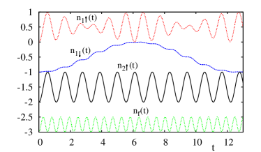
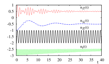
Figure 2: Time-dependent occupancies $n_{i\sigma}(t)$ of both quantum dots [as indicated] and $n_{f}(t)$ for $\lambda_{1}=\lambda_{2}=4$, $\varepsilon_{1,2}=0$, assuming the initial conditions $n_{i\sigma}(0)=0=n_{f}(0)$, and $\Gamma_{N}=0$ (upper panel), $\Gamma_{N}=0.1$ (bottom panel).

Figure 2 shows the time-dependent occupancies computed numerically for $\lambda_{1}=4=\lambda_{2}$. Results nearly coincide with the approximate formulas (28,29). The spin-$\downarrow$ occupancy of QD₁ has a similar form as for $\lambda_{1}=0$ case, but the oscillations are slower with the period equal to $2\pi/\Delta$. Note, that the oscillations of $n_{1\sigma}(t)$ are substantially different for each spin. In the time-dependent occupancy $n_{1\uparrow}(t)$ we observe superposition of two oscillations: the fast ones, with the period equal to $\sqrt{2}\pi/\Delta$, and the amplitude oscillations, with the time period equal to $2\pi$ (related to the proximitized QD₁ in absence of the Majorana modes). In contrast to that, the opposite spin occupancy $n_{1\downarrow}(t)$ oscillates with the period equal approximately to $4\pi$.

Figure 3: The time-dependent occupancies $n_{1\sigma}(t)$ obtained for the same set of model parameters as in Fig. 2. To clarify the behavior of $n_{1\uparrow}(t)$ we show the contributions from the term $M(t)$ [curve $A$] and the last term in Eq. (III.1) [curve B].

In Fig. 3 we show $n_{1\sigma}(t)$ obtained for the strong coupling $\lambda_{1}=4$ in the unbiased heterostructure, assuming $\Gamma_{N}\neq 0$. The dotted line represents contribution to $n_{1\uparrow}(t)$ from the term $M(t)$, Eq. (20). We observe its damped oscillations caused by the coupling $\Gamma_{N}$. The broken solid line represents a contribution due to the coupling of QD₁ to a continuous spectrum of the normal lead. The total sum of these contributions gives the resulting time-dependent occupancy $n_{1\uparrow}(t)$ displayed by the thin solid line. The stationary limit value $n_{1\uparrow}(t\rightarrow\infty)=0.5$ is approached after a sequence of quantum oscillations with the exponentially suppressed amplitude. Performing similar calculations for $n_{1\downarrow}(t)$ we get the result presented by the thick solid line.

III.3 On-dot pairing

Time-dependent electron populations of the individual quantum dots are further interrelated with development of the local and nonlocal pairings. Let us study this issue, first considering the singlet pairing

$$C_{11}(t)\equiv\left<\hat{d}_{1\downarrow}(t)\hat{d}_{1\uparrow}(t)\right>$$ (32)

induced on QD₁ via its proximity to the (trivial) bulk superconductor. We can analytically determine $C_{11}(t)$ using the inverse Laplace transforms of the operators $\hat{d}_{1\sigma}(s)$ and following the procedure, analogous to calculations of the charge occupancy $n_{1\sigma}(t)$. For the initially empty quantum dots and $\varepsilon_{i\sigma}=0$ the on-dot pairing (32) is given by

$$C_{11}(t)=D(t)+i\Gamma_{N}\Delta\int_{-\infty}^{\infty}\frac{d\epsilon}{2\pi}\left[f_{N}(\epsilon)D_{1}(\epsilon,t)+D_{2}(\epsilon,t)\right]$$ (33)

with function $D(t)$ and $D_{1,2}(\epsilon,t)$ presented explicitly by equations (60-62) in Appendix A.

We notice absence of any term dependent on $\lambda_{2}$. It means that electron pairing induced at QD₁ is completely unaffected by the second QD₂. The pairing function (33) depends on the initial filling of QD₁, whereas it has no dependence on $n_{f}(0)$ despite appearance of the operators $\hat{f}(0)$ and $\hat{f}^{\dagger}(0)$ in the Laplace transform of $\hat{d}_{1\uparrow}(s)$. Such terms yield the following result [see the last part of (60)]

$$\langle\left(\hat{f}(0)+\hat{f}^{\dagger}(0)\right)^{2}\rangle\frac{i\Delta\lambda_{1}^{2}}{2}{\cal{L}}^{-1}\left\{\frac{1}{H_{2}(s)}\right\}(t){\cal{L}}^{-1}\left\{\frac{s+g}{H_{2}(s)}\right\}(t),$$ (34)

which indeed is independent on $n_{f}(0)$.

For $\Gamma_{N}=0$ and initially empty QD₁ the pairing correlation function $C_{11}(t)$ is purely imaginary. It can be written in the following simple form

$$C_{11}(t) = -\frac{i}{2}\left[\frac{\lambda_{1}^{2}}{\Delta^{2}+2\lambda_{1}^{2}}\sin{\left(t\Delta\right)}\right.$$

$$+ \frac{\Delta^{2}+\lambda_{1}^{2}}{\Delta^{2}+2\lambda_{1}^{2}}\sin{\left(t\Delta\right)\cos{\left(t\sqrt{\Delta^{2}+2\lambda_{1}^{2}}\right)}}$$

$$+ \left.\frac{\Delta}{\sqrt{\Delta^{2}+2\lambda_{1}^{2}}}\cos{\left(t\Delta\right)\sin{\left(t\sqrt{\Delta^{2}+2\lambda_{1}^{2}}\right)}}\right],$$

representing a combination of the oscillations with frequencies $\Delta$ and $\sqrt{\Delta^{2}+2\lambda_{1}^{2}}$, respectively. For $\lambda_{1}\gg\Delta$, we the oscillations have the small period $\sim 2\pi/\sqrt{\Delta^{2}+2\lambda_{1}^{2}}$ and the amplitude modulated by another periodicity $4\pi$. In this case $C_{11}(t)\approx-\frac{i}{2}\sin{\left(t\Delta\right)}\cos^{2}{\left(\frac{t}{2}\sqrt{\Delta^{2}+2\lambda_{1}^{2}}\right)}$.

For the small coupling $\lambda_{1}$ we can neglect the terms proportional (and of higher order) to $\left(\frac{\lambda_{1}}{\Delta}\right)^{2}$ and get $C_{11}(t)\approx-\frac{i}{2}\sin{\left(2t\Delta\right)}$. This result is identical with the case when QD₁ is coupled only to the superconducting lead, cf. [46, 45]. For $\Gamma_{N}\neq 0$ the on-dot pairing becomes complex function. Its real part originates from the last term in Eq. (III.1) contributed by a continuous spectrum of the normal lead. This part depends on the Fermi level of the normal lead, see Eq. (A3).

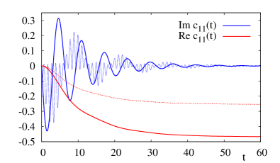
Figure 4: The complex pairing function $C_{11}(t)$ induced at QD₁ obtained for the same set of model parameters as in the bottom panel in Fig. 2 (solid lines) and in absence of the topological nanowire, $\lambda_{1}=0$, (dashed curves).

Figure 4 shows the time-dependent $C_{11}(t)$ obtained for the unbiased setup ($\mu=0$). We observe an oscillating structure of the imaginary part, similar to the behavior of $n_{1\uparrow}(t)$. This is related to the transient charge current, flowing through QD₁. These oscillations are damped, because of a continuum states responsible for the relaxation processes at QD₁. On the other hand, the real part evolves monotonously to its asymptotic (negative) value. For comparison, we also plot the complex function $C_{11}(t)$ for the case $\lambda_{1}=0$, i.e. when QD₁ is embedded only between the normal and superconducting leads [46]. The structure of $\mbox{\rm Im}C_{11}(t)$ manifests the high frequencies oscillations $\sim\sqrt{\Delta^{2}+2\lambda_{1}^{2}}$ coexisting with the beats, with frequency $\sim\Delta$. Note, that for vanishing $\lambda_{1}$ the imaginary part of $C_{11}(t)$ exhibits only one component oscillations with the frequency equal to $\Delta$.

III.4 Inter-dot pairing

We now consider the nonlocal electron pairing induced between the spatially distant quantum dots. In analogy to the previous subsection, we focus on the singlet pairing

$$C_{12}(t)\equiv\left<\hat{d}_{1\downarrow}(t)\hat{d}_{2\uparrow}(t)\right>.$$ (36)

In practice this sort of electron pairing could be detected via the crossed Andreev reflections in hybrid structures with an additional electrode contacted to QD₂. Let us remark, that $C_{12}(t)$ originates from the local pairing of QD₁ electrons, which is further extended onto QD₂ by the Majorana quasiparticles. Technically this is provided by the operators $\hat{f}^{(\dagger)}(0)$ appearing in the Laplace transforms of $\hat{d}_{1\downarrow}(s)$ and $\hat{d}_{2\uparrow}(s)$ [see Eqs. (8,16)]. For $\varepsilon_{i\sigma}=0$ we find

$$C_{12}(t) = i\lambda_{1}\lambda_{2}\Delta\left[\frac{1}{2}-n_{f}(0)\right]$$

$$\times {\cal{L}}^{-1}\left\{\frac{1}{H_{2}(s)}\right\}(t){\cal{L}}^{-1}\left\{\frac{1}{s^{2}+2\lambda_{2}^{2}}\right\}(t).$$

In the limit $\Gamma_{N}=0$ the pairing $C_{12}(t)$ simplifies to

$$C_{12}(t) = \frac{i\lambda_{1}\Delta}{\sqrt{2}(\Delta^{2}+2\lambda_{1}^{2})}\left[1-2n_{f}(0)\right]$$

$$\times \sin{\left(\sqrt{2}t\lambda_{2}\right)}\sin^{2}{\left(\frac{t}{2}\sqrt{\Delta^{2}+2\lambda_{1}^{2}}\right)}.$$

For finite $\Gamma_{N}$, we obtain

$$C_{12}(t) = \frac{i\lambda_{1}\Delta}{2\sqrt{2}}\left[1-2n_{f}(0)\right]\sin{\left(\sqrt{2}t\lambda_{2}\right)}$$

$$\times \frac{e^{-at}+e^{-bt}\left[\frac{a-b}{c}\sin{\left(ct\right)}-\cos{\left(ct\right)}\right]}{(b-a)^{2}+c^{2}},$$

where the parameters $a,b,c$ correspond to three roots $s_{i}$ ($i=1,2,3$) of the cubic equation $H_{2}(s_{i})=0$. One of these roots, say $s_{1}$, is real and it defines the positive valued parameter $a>0$ via $s_{1}=-a$. The other parameters, $b$ and $c$, are related with the conjugated roots $s_{2}=s_{3}^{\star}$. They are expressed as $s_{2/3}=-b\pm ic$, where $b>0$.

Equation (III.4) implies, that the inter-dot pairing (36) does not depend on the initial charge $n_{i\sigma}(0)$ of the quantum dots. Furthermore, $C_{12}(t)$ has no explicit dependence on the voltage $\mu$ applied across QD₁ between the external leads because the operators $\hat{c}_{{\bf k}\sigma}(0)$ do not appear simultaneously in $\hat{d}_{1\downarrow}(t)$ and $\hat{d}_{2\uparrow}(t)$. Influence of the normal lead, however, enters indirectly through the roots $s_{1-3}$ (where $a$, $b$ and $c$ depend on $\Gamma_{N}$). We observe that for $\Gamma_{N}=0$ the amplitude of $C_{12}(t)$ oscillations diminishes upon increasing $\lambda_{1}$, whereas for $\Gamma_{N}\neq 0$ we observe similar behavior, though with the damped oscillations. In general, the nonlocal pairing $C_{12}(t)$ is also sensitive to the energy levels $\varepsilon_{i\sigma}$ of both quantum dots.

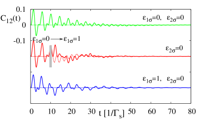
Figure 5: The complex inter-dot pairing function $C_{12}(t)$ obtained for $\lambda_{1}=1=\lambda_{2}$, $\Gamma_{N}=0.2$ and several energy levels, as indicated. Dashed lines refer to the real and solid curves to the imaginary parts of $C_{12}(t)$, respectively. The middle plot (green color) presents evolution of $C_{12}(t)$, imposing a sudden change of the energy level $\varepsilon_{1\sigma}=0$ to $\varepsilon_{1\sigma}=1$ at $t=10$.

We notice, that the inter-dot pairing survives only in the transient region (see Fig. 5). The time-dependent profile of this complex pairing function $C_{12}(t)$ is sensitive to specific values of the energy levels. Additional effects can arise from the quantum quenches. The middle plot in Fig. 5 displays the evolution of $C_{12}(t)$ after a sudden change of $\varepsilon_{1\sigma}$ imposed at $t=10$. This quench substantially affects the real and imaginary parts of the nonlocal pairing $C_{12}(t)$. We have checked, however, that signatures of the nonlocal pairing are completely absent if such quantum quench occurs outside the transient regime. This observation emphasises the subtle importance of transient phenomena, which enable mutual correlations between the spatially distant quantum dots. Such dynamical non-local effects would be observable in the crossed Andreev transmission, and could possibly arise via the single particle teleportation as well.

III.5 Triplet pairing

Finally let us consider the mixed pairing between QD₂ and the topological superconducting nanowire

$$C_{2f}(t)=\left<\hat{d}_{2\uparrow}(t)\hat{f}(t)\right>.$$ (40)

This triplet pairing is associated with leakage of the Majorana mode onto the side-attached quantum dot (here on QD₂, but similar process takes place on QD₁ as well). Let us recall, that from both operators $\hat{d}_{2\uparrow}(s)$ and $\hat{f}(s)$ only the latter one depends on $\hat{c}_{{\bf k}\sigma}^{(\dagger)}(0)$. For this reason the mixed pairing (40) is not dependent on the normal lead electrons and thereby to the bias voltage $\mu$.

In what follows, we focus on the initially empty dot $n_{2\uparrow}(0)=0$ and $n_{f}(0)=0$, assuming the isotropic couplings $\lambda_{1}=\lambda_{2}\equiv\lambda$. Under such conditions we obtain (for $\varepsilon_{i\sigma}=0$)

$$C_{2f}(t) = \frac{i}{2}\sin{\left(\sqrt{2}\lambda t\right)}\left[\cos^{2}{\left(\frac{\lambda t}{\sqrt{2}}\right)}\right.$$ (41)

$$+ \left.\lambda^{2}{\cal{L}}^{-1}\left\{\frac{sg+\Delta^{2}+g^{2}}{(s^{2}+2\lambda^{2})H_{2}(s)}\right\}(t)\right].$$

For $\Gamma_{N}=0$ this formula (41) simplifies to

$$C_{2f}(t)=\frac{i\sin{\left(\sqrt{2}\lambda t\right)}}{2(\Delta^{2}+2\lambda^{2})}\left[\Delta^{2}+2\lambda^{2}\cos^{2}{\left(\frac{\sqrt{\Delta^{2}+2\lambda^{2}}}{2}t\right)}\right],$$ (42)

revealing the oscillating behavior. This analytical result (42) is valid when the quantum dots interconnected through the Majorana quasiparticles are not coupled to a continuous spectrum of the normal lead that could activate the relaxation processes. It appears, however, that even in the case $\Gamma_{N}\neq 0$ the mixed pairing function (41) oscillates against time with non-vanishing amplitude. To observe it, we evaluated the pairing function (41) in the large $t$ limit

$$C_{2f}(t) = \frac{i}{2}\sin{\left(\sqrt{2}\lambda t\right)}\left[\cos^{2}{\left(\frac{\lambda t}{\sqrt{2}}\right)}\right.$$ (43)

$$+ 2\lambda^{2}g\left.\mbox{\rm Re}\left(\frac{e^{i\sqrt{2}\lambda t}s_{16}}{s_{12}s_{13}s_{14}s_{15}}\right)\right].$$

Here $s_{nm}=s_{n}-s_{m}$, where $s_{1}=i\sqrt{2}\lambda$, $s_{2}=-s_{1}$, $s_{3}=-a$, $s_{4/5}=-b\pm ic$, $s_{6}=-(\Delta^{2}+g^{2})/g$, where $s_{3}$, $s_{4}$, $s_{5}$ are the roots of the cubic equation $H_{2}(s_{i})=0$ and $a$, $b$ are real positive parameters. In the large $t$ limit this pairing function is purely imaginary and it has oscillating character. The formula presented in Eq. (43) is valid for $\varepsilon_{1\sigma}=0=\varepsilon_{2\sigma}$. Otherwise, the operators $\hat{d}_{2\uparrow}(s)$ and $\hat{f}(s)$ could depend on the energy levels $\varepsilon_{i\sigma}$ affecting the pairing function $C_{2f}(t)$. In particular, influence of QD₁ on the triplet pairing $C_{2f}(t)$ is incorporated via the operator $\hat{f}$.

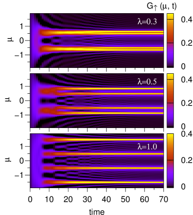
Figure 6: Time-resolved differential conductance of the charge current flowing through the first quantum dot (QD₁) induced by the voltage bias $\mu$ applied between the normal and superconducting leads. Panels refer to the different couplings $\lambda_{1}$ of QD₁ to the topological superconductor, as indicated.

IV Differential tunneling conductance

In this section we study the differential conductance $G_{\sigma}(\mu,t)=\frac{\partial}{\partial\mu}j_{N\sigma}(t)$ of the time-dependent current $j_{N\sigma}(t)$, flowing between QD₁ and the normal lead. For convenience we express $G_{\sigma}(\mu,t)$ in units of $2e^{2}/h$ and investigate its dependence on the voltage $\mu$. The tunneling current can be determined from the evolution of the total number of electrons in the normal electrode. For our setup it can be written as [46]

$$j_{N\sigma}(\mu,t)=2\mbox{\rm Im}\sum_{\bf k}V_{\bf k}e^{-i\varepsilon_{\bf k}t}\left<\hat{d}_{1\sigma}^{\dagger}(t)\hat{c}_{{\bf k}\sigma}(0)\right>-\Gamma_{N}n_{1\sigma}(t).$$ (44)

Substituting the inverse Laplace transform of $\hat{d}_{1\uparrow}(s)$ [see Eqn. (III.1)] we obtain derivative of the first term appearing in Eqn. (44) with respect to $\mu$ in the following way

$$\frac{\partial}{\partial\mu}2\mbox{\rm Im}\left(i\sum_{{\bf k},{\bf k}_{1}}V_{\bf k}V_{{\bf k}_{1}}e^{-i\varepsilon_{\bf k}t}{\cal{L}}^{-1}\left\{\frac{(s+g)H_{1}(s)}{(s-\varepsilon_{{\bf k}_{1}})H_{3}(s)}\right\}(t)\left<\hat{c}_{{\bf k}_{1}\uparrow}^{\dagger}(t)\hat{c}_{{\bf k}\uparrow}(0)\right>\right)$$ (45)

$$= \frac{\partial}{\partial\mu}\frac{\Gamma_{N}}{\pi}\mbox{\rm Re}\int_{-\infty}^{\infty}d\varepsilon f_{N}(\varepsilon)e^{-i\varepsilon t}{\cal{L}}^{-1}\left\{\frac{(s+g)H_{1}(s)}{(s-\varepsilon)H_{3}(s)}\right\}(t)=\frac{\Gamma_{N}}{\pi}\mbox{\rm Re}\left(e^{-i\mu t}{\cal{L}}^{-1}\left\{\frac{(s+g)H_{1}(s)}{(s-\mu)H_{3}(s)}\right\}(t)\right).$$

In the next step we subsequently calculate $\partial n_{1\uparrow}(t)/\partial\mu$ taking into consideration only such terms which depend on the bias voltage [see Eqn. (A2)]. In result we get

$$\frac{\partial n_{1\uparrow}(t)}{\partial\mu} = \frac{\Gamma_{N}}{2\pi}\left\{\Delta^{2}\lambda_{1}^{4}\left|{\cal{L}}^{-1}\left\{\frac{s+g}{(s+i\mu)H_{3}(s)}\right\}(t)\right|^{2}+\left|{\cal{L}}^{-1}\left\{\frac{(s+g)H_{1}(s)}{(s+i\mu)H_{3}(s)}\right\}(t)\right|^{2}\right.$$ (46)

$$- \left.\Delta^{2}\left|{\cal{L}}^{-1}\left\{\frac{H_{1}(s)}{(s+i\mu)H_{3}(s)}\right\}(t)\right|^{2}-\lambda_{1}^{4}\left|{\cal{L}}^{-1}\left\{\frac{(s+g)^{2}}{(s+i\mu)H_{3}(s)}\right\}(t)\right|^{2}\right\}.$$

The definition $G_{\uparrow}(\mu,t)=\frac{\partial}{\partial\mu}j_{N\uparrow}(t)$ along with Eqs. (14,45,46) yield the information on time-dependent quasiparticle states of our hybrid structure. The relevant inverse Laplace transforms can be obtained in a form of the linear combinations of $\exp{\left(-gt\right)}$ and $\exp{\left(-s_{i}t\right)}$ with coefficients being the functions of $s_{1},...,s_{8}$, where $s_{1,2}=-g\pm i\Delta$ and $s_{3}$, $s_{4}$, $s_{5}$ ($s_{6}$, $s_{7}$, $s_{8}$) are solutions of the cubic equation $H_{1}(s)=0$ ($H_{2}(s)=0$).

Figure 6 presents the time-dependent conductance versus the bias voltage $\mu$ obtained for $\lambda_{1}=0.3$, $0.5$ and $1.0$, respectively. It shows how the quasiparticle peaks of QD₁ develop in time. For the weak couplings, $\lambda_{1}=0.3$ and $0.5$, we observe roughly two quasiparticle peaks emerging from the initial broad-structure (panels a and b in Fig. 6). Their steady-limit shape establishes at relatively long time in comparison to the results obtained for the stronger coupling, $\lambda_{1}=1.0$. After closer inspection, however, we can notice some tiny splitting between the maxima. In contrast, for the larger coupling $\lambda_{1}$ there appear four quasiparticle peaks well separated from one another. Their steady limit structure establishes pretty fast, nearly at $t\approx 10$. Duration of the transient region is thus strongly sensitive to the coupling strength $\lambda_{1}$.

In Fig. 7 we present the steady limit differential conductance $G_{\sigma}(\mu,t\rightarrow\infty)$ obtained for different couplings $\lambda_{1}=\lambda_{2}$, as indicated. Since one of the solutions, $s_{3}$ ($s_{6}$) for the cubic equation has a negative real value and the other solutions are complex (with negative real parts), we get

$$G_{\uparrow}(\mu,\infty)=\Gamma_{N}\mbox{\rm Re}\left(\frac{\phi_{1}(\mu)}{\phi_{3}(\mu)}\right)-\frac{\Gamma_{N}^{2}}{2}\left[\left|\phi_{1}(\mu)\right|^{2}\right.$$

$$- \left.\Delta^{2}\left|\phi_{2}(\mu)\right|^{2}+\lambda_{1}^{4}\left(g^{2}+\mu^{2}\right)\left(\Delta^{2}-g^{2}-\mu^{2}\right)\right]/\left|\phi_{3}\right|^{2},$$

where $\phi_{2}(\mu)=\prod_{j=3,4,5}\left(i\mu-s_{j}\right)$, $\phi_{1}(\mu)=\left(i\mu+g\right)\phi_{2}(\mu)$, and $\phi_{3}(\mu)=\prod_{j=1,2,6,7,8}\left(i\mu-s_{j}\right)$. We can approximately evaluate $G_{\uparrow}$, taking into consideration only the first term appearing in Eqn. (IV). From this analysis, we can determine positions of $G_{\uparrow}$ peaks. We observe two peaks at positive and two peaks at negative bias voltage. The internal peaks at $\mu=\pm\Delta$ are independent on $\lambda_{1}$, whereas the outer peaks appear at $\mu\simeq\pm\sqrt{\Delta^{2}+2\lambda_{1}^{2}}$. Spectral weight of the internal peaks varies from $1$ (for $\lambda_{1}=0$) to $0.5$ (for stronger couplings $\gamma_{1}$). At the same time the spectral weight of the outer peaks at $\mu=\pm\sqrt{\Delta^{2}+2\lambda_{1}^{2}}$ increases to $1$ (for $\lambda_{1}\geq 1$).

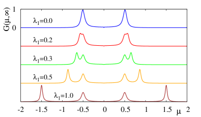
Figure 7: Steady limit of the differential conductance $G_{\uparrow}(\mu,\infty)$ obtained for $\varepsilon_{i\sigma}=0$ and several values of $\lambda_{1}$, as indicated.

The time-dependent differential conductance shown Fig. 6 and its asymptotic limit (Fig. 7) provide information about the Andreev-type states of $QD_{1}$ (due to superconducting proximity effect) obtained for the special case, when the energy level $\varepsilon_{1\sigma}=0$ coincides with the zero-energy Majorana mode. Under such circumstances, influence of the Majorana mode on the quasiparticle spectrum of QD₁ is manifested by destructive quantum interference in some analogy to Fano-type lineshapes appearing in double quantum dot T-shape configurations [49, 50, 51]. In our present case, this destructive interference shows up by a tiny dip at zero voltage for the weakly coupled heterostructure [see curves presented in Fig. 7 for $\lambda_{1}=0.1$, $0.2$ and $0.3$].

In remaining part of this section, we investigate the quasiparticle features appearing in the conductance $G_{\uparrow}(\mu,t)$ for $\varepsilon_{1\sigma}\neq 0$. In such situation the Majorana mode has a constructive influence, inducing the zero-energy quasiparticle which enhances the zero-bias conductance. This effect resembles the typical Majorana leakage on the quantum dot hybridized to the normal (metallic) electrodes [26, 27, 28, 29, 30, 31, 32, 33, 34, 35, 36, 37]. For nonzero $\varepsilon_{1\sigma}$ we obtain

$$G_{\uparrow}(\mu,t) = \Gamma_{N}\mbox{\rm Re}\left[e^{-i\mu t}{\cal{L}}^{-1}\left\{\frac{(s+i\varepsilon+g)F_{1}(s)}{(s-i\mu)F_{2}(s)}\right\}(t)\right]$$ (48)

$$- \frac{\Gamma_{N}^{2}}{2}\left[\left|{\cal{L}}^{-1}\left\{\frac{(s+i\varepsilon+g)F_{1}(s)}{(s-i\mu)F_{2}(s)}\right\}(t)\right|^{2}\right.$$

$$+ \Delta^{2}\lambda_{1}^{4}\left|{\cal{L}}^{-1}\left\{\frac{s+i\varepsilon+g}{(s-i\mu)F_{2}(s)}\right\}(t)\right|^{2}$$

$$- \Delta^{2}\left|{\cal{L}}^{-1}\left\{\frac{F_{1}(s)}{(s+i\mu)F_{2}(s)}\right\}(t)\right|^{2}$$

$$- \lambda_{1}^{4}\left.\left|{\cal{L}}^{-1}\left\{\frac{(s+g)^{2}+\varepsilon^{2}}{(s+i\mu)F_{2}(s)}\right\}(t)\right|^{2}\right],$$

where $F_{1}(s)=s^{3}+2gs^{2}+s(\varepsilon^{2}+\Delta^{2}+g^{2}+\lambda_{1}^{2})-\lambda_{1}^{2}(i\varepsilon-g)$ and $F_{2}(s)=(s^{2}+2gs+\varepsilon^{2}+\Delta^{2}+g^{2})(s^{3}+2gs^{2}+s(g^{2}+\varepsilon^{2}+\Delta^{2}+2\lambda_{1}^{2})+2\lambda_{1}^{2}g)$.

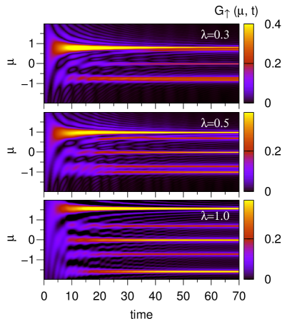
Figure 8: The time-dependent differential conductance $G_{\uparrow}(\mu,t)$ obtained for non-zero energy level of the first quantum dot, $\varepsilon_{1\sigma}=1.0$, and different values of the coupling $\lambda_{1}$.

Figure 8 shows the time-dependent differential conductance $G_{1\uparrow}(\mu,t)$ obtained for non-zero value of the QD₁ energy level, $\varepsilon_{1\sigma}=0.5$, and several values of the coupling $\lambda_{1}$. In the stationary limit, ($t\rightarrow\infty$), the height of zero-energy peak tends to $0.5$ which is typical fractional value initially predicted for the leaking Majorana mode [21, 26, 27]) for arbitrary $\lambda_{1}$. Its width increases here upon increasing the coupling $\lambda_{1}$ as can be seen in the stationary limit presented in Fig. 9.

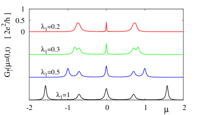
Figure 9: Steady limit of the conductance $G_{\uparrow}(\mu,t=\infty)$ obtained for several values of $\lambda_{1}$ (as indicated) and $\varepsilon_{1\sigma}=1$.

To estimate the time interval in which the zero-energy Majorana mode leaks onto QD₁ we introduce the phenomenological parameter $\tau$ defined by [41]

$$G_{\uparrow}(0,t)=G_{\uparrow}(0,\infty)\left[1-e^{-t/t}\right].$$ (49)

This parameter $\tau$ characterizes the time-scale, over which the zero-bias conductance approaches the stationary limit value $G_{\uparrow}(0,\infty)$. We computed $\tau$ for two different energy levels $\varepsilon_{1\sigma}$ and several values of the coupling $\lambda_{1}$. Fig. 10 presents the zero-bias conductance $G_{\uparrow}(\mu=0,t)$ for $\varepsilon_{1\sigma}=0.5$ (solid lines) and $1.0$ (dashed curves), using $\lambda_{1}$ specified in the table 1. We found $\tau\approx 15$, $5$, $2.5$, $2.0$ (expressed in units $\frac{1}{\Gamma_{N}}$) for the couplings $\lambda_{1}=0.2$, $0.4$, $1$ and $4$, respectively. Similarly, for another energy level, $\varepsilon_{1\sigma}=1$, we estimated the leakage time-scales $\tau\approx 3.2$, $2.3$, $2.2$. We thus conclude, that development of the zero-energy Majorana mode on QD₁ occurs faster upon increasing the coupling $\lambda_{1}$.

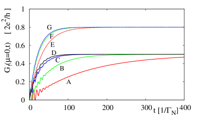
Figure 10: The zero-bias differential conductance $G_{\uparrow}(\mu=0,t)$ varying against time for $\varepsilon_{1\sigma}=0.5$ (solid lines) and $\varepsilon_{1\sigma}=1$ (dashed lines) using different values of $\lambda$ listed in table 1.

Curve	$\lambda_{1}[1/\Gamma_{S}]$	$\varepsilon_{1\sigma}[\Gamma_{S}]$	$\tau[1/\Gamma_{N}]$
A	0.2	0.5	15
B	0.4	0.5	5
C	1.0	0.5	2.5
D	4.0	0.5	2.0
E	1.0	1.0	3.2
F	2.0	1.0	2.3
G	3.0	1.0	2.2

Table 1: Time-scale $\tau$ of the Majorana leakage obtained for several couplings $\lambda_{1}$ and different energy level $\varepsilon_{1\sigma}$ of QD₁.

Summarizing this section, we emphasize that quasiparticles emerging on QD₁ (presented in Figs 8 and 9) represent the trivial Andreev bound states (at finite voltage $\mu$) coexisting with the topological (zero-bias) feature. Their formation occurs over some characteristic time-scale $\tau$ [see Table 1] and is accompanied by the damped quantum oscillations. Buildup of the quasiparticles is predominantly controlled by the coupling of QD₁ to a continuous spectrum of the metallic lead, but spectral weights and energies of such quasiparticles depend on the energy level $\varepsilon_{1\sigma}$ of QD₁, what indirectly affects the profile of damped quantum oscillations observed in the transient regime.

V Summary and outlook

We have studied the local and nonlocal transient phenomena of the hybrid structure composed of two quantum dots attached to opposite sides to the topological superconducting nanowire. We have shown that in a steady-state limit these spatially distant quantum dots interconnected through the Majorana edge-modes develop the quasiparticle spectra independent of one another. Despite the lack of static cross-correlations, however, we have found dynamical nonlocal effects transmitted between the dots surviving over a finite time interval. These effects are apparent in the inter-dot electron pairing, both for the singlet and triplet channels, which could be detectable in the crossed Andreev reflection spectroscopy.

We have also investigated gradual development of the quasiparticle states of QD₁, focusing on signatures of the Majorana mode. We have found coexistence of the (trivial) Andreev bound states with the (topological) zero-energy feature. Emergence of these quasiparticles can be empirically verified by time-resolved differential conductance of the tunneling current across QD₁ induced by the bias voltage applied between the external metallic and superconducting leads. For the energy level $\varepsilon_{1\sigma}=0$, the Majorana mode imprints a tiny dip at zero voltage, originating from its destructive quantum interference on the spectrum of QD₁. This effect is analogous to the Fano-type interference patterns observed in T-shape configurations of double quantum dot junctions [49, 50, 51]. Otherwise, i.e. for $\varepsilon_{1\sigma}\neq 0$, the Majorana mode induces the zero-energy conductance peak. In the latter case the leakage of Majorana mode yields a fractional value of the zero-bias differential conductance, Fig. 9.

Our analysis relied on the assumption of very large pairing gap $\Delta_{sc}$ of the superconducting lead. In realistic situations, one should consider the influence of electronic spectrum outside this pairing gap (which for conventional superconductors is typically a fraction of meV). The influence of such continuum has been taken into account for superconducting nanostructures in the absence of the topological phase using a number of many-body techniques [52, 53, 54, 55, 56, 57, 58] suitable to capture also the correlation effects. These methods could be adopted to the present setup. The impact of the quasiparticles from outside the pairing gap would contribute to the relaxation processes, effectively reducing the relevant time scales in the problem. Another important issue could be associated with qualitative changeover of the trivial (Andreev) and topological (Majorana) states in response to the quantum quench [59]. This challenging topic, however, is beyond the scope of the present study.

For possible empirical verification, we have evaluated the time-scale needed for emergence of the trivial (Andreev) and topological (Majorana) bound states. In typical realizations of superconducting hybrid structures (where the couplings $\Gamma_{N,S}$ of the quantum dots to external leads are $\sim$ meV) the duration of the transient effects would cover nanoseconds region. Currently available tunneling spectroscopies should be able to detect the nonlocal cross-correlations between the spatially distant quantum dots embedded into the setup presented in Fig 1. Detailed knowledge of such effects might be important for reliable control of the braiding protocols using conventional and/or topological superconducting quantum bits [60, 61].

Appendix A Time-dependent expectation values

Let us calculate the charge occupancy of QD₁. Using the expression (III.1) for $\hat{d}_{1\uparrow}(s)$ we obtain

$$n_{1\uparrow}(t) = \left<{\cal{L}}^{-1}\left\{\hat{d}_{1\uparrow}^{\dagger}(s)\right\}{\cal{L}}^{-1}\left\{\hat{d}_{1\uparrow}(s)\right\}\right>$$

$$= \left[1-n_{1\uparrow}(0)\right]\lambda_{1}^{4}\left({\cal{L}}^{-1}\left\{\frac{(s+g)^{2}}{H_{3}(s)}\right\}(t)\right)^{2}+n_{1\uparrow}(0)\left({\cal{L}}^{-1}\left\{\frac{(s+g)H_{1}(s)}{H_{3}(s)}\right\}(t)\right)^{2}$$

$$+ \left[1-n_{1\downarrow}(0)\right]\Delta^{2}\left({\cal{L}}^{-1}\left\{\frac{H_{1}(s)}{H_{3}(s)}\right\}(t)\right)^{2}+n_{1\downarrow}(0)\Delta^{2}\lambda_{1}^{4}\left({\cal{L}}^{-1}\left\{\frac{s+g}{H_{3}(s)}\right\}(t)\right)^{2}$$

$$+ \left<\hat{f}^{\dagger}(0)+\hat{f}(0)\right>\left<\hat{f}(0)+\hat{f}^{\dagger}(0)\right>\frac{\lambda_{1}^{2}}{2}\left({\cal{L}}^{-1}\left\{\frac{(s+g)}{H_{2}(s)}\right\}(t)\right)^{2}+\sum_{{\bf k},{\bf k}_{1}}V_{\bf k}V_{{\bf k}_{1}}\left<{\cal{L}}^{-1}\left\{S_{\bf k}^{\dagger}(s)\right\}(t){\cal{L}}^{-1}\left\{S_{{\bf k}_{1}}(s)\right\}(t)\right>$$

where $H_{1}(s)$, $H_{2}(s)$, $H_{3}(s)$ and $S_{\bf k}(s)$ are defined in Eqs. (10,11,12,15). The first five terms can be rewritten in the form given by Eq. (17) and calculation of the last term can be performed as follows

$$\sum_{{\bf k},{\bf k}_{1}}V_{\bf k}V_{{\bf k}_{1}}\left<{\cal{L}}^{-1}\left\{\Delta\frac{\hat{c}_{{\bf k}\downarrow}(0)H_{1}(s)}{(s+i\varepsilon_{\bf k})H_{3}(s)}+i\frac{\hat{c}_{{\bf k}\uparrow}^{\dagger}(0)(s+g)H_{1}(s)}{(s-i\varepsilon_{\bf k})H_{3}(s)}+\Delta\lambda_{1}^{2}\frac{\hat{c}_{{\bf k}\downarrow}^{\dagger}(0)(s+g)}{(s-i\varepsilon_{\bf k})H_{3}(s)}-i\lambda_{1}^{2}\frac{\hat{c}_{{\bf k}\uparrow}(0)(s+g)^{2}}{(s+i\varepsilon_{\bf k})H_{3}(s)}\right\}(t)\right.$$

$$\times \left.{\cal{L}}^{-1}\left\{\Delta\frac{\hat{c}^{\dagger}_{{\bf k}_{1}\downarrow}(0)H_{1}(s)}{(s-i\varepsilon_{{\bf k}_{1}})H_{3}(s)}-i\frac{\hat{c}_{{\bf k}_{1}\uparrow}(0)(s+g)H_{1}(s)}{(s+i\varepsilon_{{\bf k}_{1}})H_{3}(s)}+\Delta\lambda_{1}^{2}\frac{\hat{c}_{{\bf k}_{1}\downarrow}(0)(s+g)}{(s+i\varepsilon_{{\bf k}_{1}})H_{3}(s)}+i\lambda_{1}^{2}\frac{\hat{c}_{{\bf k}_{1}\uparrow}^{\dagger}(0)(s+g)^{2}}{(s-i\varepsilon_{{\bf k}_{1}})H_{3}(s)}\right\}(t)\right>$$

$$= \sum_{{\bf k},{\bf k}_{1}}V_{\bf k}V_{{\bf k}_{1}}\left\{\Delta^{2}\left<\hat{c}_{{\bf k}\downarrow}(0)\hat{c}_{{\bf k}_{1}\downarrow}^{\dagger}(0)\right>{\cal{L}}^{-1}\left\{\frac{H_{1}(s)}{(s+i\varepsilon_{\bf k})H_{3}(s)}\right\}(t){\cal{L}}^{-1}\left\{\frac{H_{1}(s)}{(s-i\varepsilon_{{\bf k}_{1}})H_{3}(s)}\right\}(t)\right.$$

$$+ \left<\hat{c}_{{\bf k}\uparrow}^{\dagger}(0)\hat{c}_{{\bf k}_{1}\uparrow}(0)\right>{\cal{L}}^{-1}\left\{\frac{(s+g)H_{1}(s)}{(s-i\varepsilon_{\bf k})H_{3}(s)}\right\}(t){\cal{L}}^{-1}\left\{\frac{(s+g)H_{1}(s)}{(s+i\varepsilon_{{\bf k}_{1}})H_{3}(s)}\right\}(t)$$

$$+ \Delta^{2}\lambda_{1}^{4}\left<\hat{c}_{{\bf k}\downarrow}^{\dagger}(0)\hat{c}_{{\bf k}_{1}\downarrow}(0)\right>{\cal{L}}^{-1}\left\{\frac{(s+g)}{(s-i\varepsilon_{\bf k})H_{3}(s)}\right\}(t){\cal{L}}^{-1}\left\{\frac{(s+g)}{(s+i\varepsilon_{{\bf k}_{1}})H_{3}(s)}\right\}(t)$$

$$+ \left.\lambda_{1}^{4}\left<\hat{c}_{{\bf k}\uparrow}(0)\hat{c}_{{\bf k}_{1}\uparrow}^{\dagger}(0)\right>{\cal{L}}^{-1}\left\{\frac{(s+g)^{2}}{(s+i\varepsilon_{\bf k})H_{3}(s)}\right\}(t){\cal{L}}^{-1}\left\{\frac{(s+g)^{2}}{(s-i\varepsilon_{{\bf k}_{1}})H_{3}(s)}\right\}(t)\right\}$$

$$= \frac{\Gamma_{N}}{2\pi}\int_{-\infty}^{\infty}d\varepsilon\left\{\Delta^{2}\left[1-f_{N}(\varepsilon)\right]{\cal{L}}^{-1}\left\{\frac{H_{1}(s)}{(s+i\varepsilon)H_{3}(s)}\right\}(t){\cal{L}}^{-1}\left\{\frac{H_{1}(s)}{(s-i\varepsilon)H_{3}(s)}\right\}(t)\right.$$

$$+ f_{N}(\varepsilon){\cal{L}}^{-1}\left\{\frac{(s+g)H_{1}(s)}{(s-i\varepsilon)H_{3}(s)}\right\}(t){\cal{L}}^{-1}\left\{\frac{(s+g)H_{1}(s)}{(s+i\varepsilon)H_{3}(s)}\right\}(t)$$

$$+ \Delta^{2}\lambda_{1}^{4}f_{N}(\varepsilon){\cal{L}}^{-1}\left\{\frac{(s+g)}{(s-i\varepsilon)H_{3}(s)}\right\}(t){\cal{L}}^{-1}\left\{\frac{(s+g)}{(s+i\varepsilon)H_{3}(s)}\right\}(t)$$

$$+ \left.\lambda_{1}^{4}\left[1-f_{N}(\varepsilon)\right]{\cal{L}}^{-1}\left\{\frac{(s+g)^{2}}{(s+i\varepsilon)H_{3}(s)}\right\}(t){\cal{L}}^{-1}\left\{\frac{(s+g)^{2}}{(s-i\varepsilon)H_{3}(s)}\right\}(t)\right\}.$$

This expression can be simply transfromed to the form given in Eq. (17), where we have introduced the Fermi-Dirac distribution function $f_{N}(\varepsilon)=\left[1+\exp{\left(\varepsilon/k_{B}T\right)}\right]^{-1}$.

Performing similar calculations for $n_{1\downarrow}(t)$ we obtain

$$n_{1\downarrow}(t)=n_{1\uparrow}(0)N_{\uparrow}(t)+n_{1\downarrow}(0)N_{\downarrow}(t)+N(t)+\frac{\Gamma_{N}}{2\pi}\int_{-\infty}^{\infty}d\varepsilon\left[f_{N}(\varepsilon)\Psi_{1}(\varepsilon,t)+\Psi_{2}(\varepsilon,t)\right],$$ (52)

where

$$N_{\uparrow}(t) = \Delta^{2}\lambda_{1}^{4}\left({\cal{L}}^{-1}\left\{\frac{(s+g)^{2}}{H_{3}(s)}\right\}(t)\right)^{2}-\Delta^{2}\left({\cal{L}}^{-1}\left\{\frac{H_{1}(s)}{H_{3}(s)}\right\}(t)\right)^{2},$$ (53)

$$N_{\downarrow}(t) = \left({\cal{L}}^{-1}\left\{\frac{\Delta^{2}H_{1}(s)}{(s+g)H_{3}(s)}-\frac{1}{s+g}\right\}(t)\right)^{2}-\Delta^{2}\lambda_{1}^{4}\left({\cal{L}}^{-1}\left\{\frac{1}{H_{3}(s)}\right\}(t)\right)^{2},$$ (54)

$$N(t) = \Delta^{2}\left({\cal{L}}^{-1}\left\{\frac{H_{1}(s)}{H_{3}(s)}\right\}(t)\right)^{2}+\Delta^{4}\lambda_{1}^{4}\left({\cal{L}}^{-1}\left\{\frac{1}{H_{3}(s)}\right\}(t)\right)^{2}+\frac{\Delta^{2}\lambda_{1}^{2}}{2}\left({\cal{L}}^{-1}\left\{\frac{1}{H_{2}(s)}\right\}(t)\right)^{2},$$ (55)

and

$$\Psi_{1}(\varepsilon,t) = \Delta^{2}\lambda_{1}^{4}\left|{\cal{L}}^{-1}\left\{\frac{s+g}{(s+i\varepsilon)H_{3}(s)}\right\}(t)\right|^{2}-\Delta^{2}\lambda_{1}^{4}\left|{\cal{L}}^{-1}\left\{\frac{1}{(s+i\varepsilon)H_{3}(s)}\right\}(t)\right|^{2}$$ (56)

$$+ \left|{\cal{L}}^{-1}\left\{\left(\frac{\Delta^{2}H_{1}(s)}{(s+g)H_{3}(s)}-\frac{1}{s+g}\right)\frac{1}{s-i\varepsilon}\right\}(t)\right|^{2}-\Delta^{2}\left|{\cal{L}}^{-1}\left\{\frac{H_{1}(s)}{(s-i\varepsilon)H_{3}(s)}\right\}(t)\right|^{2}$$ (57)

$$\Psi_{2}(\varepsilon,t) = \Delta^{4}\lambda_{1}^{4}\left|{\cal{L}}^{-1}\left\{\frac{1}{(s+i\varepsilon)H_{3}(s)}\right\}(t)\right|^{2}+\Delta^{2}\left({\cal{L}}^{-1}\left\{\frac{H_{1}(s)}{(s+i\varepsilon)H_{3}(s)}\right\}(t)\right|^{2}.$$ (58)

Note, that $n_{1\downarrow}(t)$ does not depend on $\lambda_{2}$, $\varepsilon_{2}$.

The intra-dor pairing function (32) can be computed, using the Laplace transforms $\hat{d}_{1\uparrow}(s)$ and $\hat{d}_{1\downarrow}(s)$ expressed in equations (III.1,16). Following the precudure discussed above for the charge occupancies we finally obtain (assuming the initial empty dots)

$$\left<\hat{d}_{1\downarrow}(t)\hat{d}_{1\uparrow}(t)\right>=D(t)+i\frac{\Gamma_{N}\Delta}{2\pi}\int_{-\infty}^{\infty}\left[f_{N}(\varepsilon)D_{1}(\varepsilon,t)+D_{2}(\varepsilon,t)\right],$$ (59)

where

$$D(t) = i\Delta\left[\lambda_{1}^{4}{\cal{L}}^{-1}\left\{\frac{s+g}{H_{3}(s)}\right\}(t){\cal{L}}^{-1}\left\{\frac{(s+g)^{2}}{H_{3}(s)}\right\}(t)+{\cal{L}}^{-1}\left\{\frac{H_{1}(s)}{H_{3}(s)}\right\}(t){\cal{L}}^{-1}\left\{\frac{\Delta^{2}H_{1}(s)-H_{3}(s)}{(s+g)H_{3}(s)}\right\}(t)\right.$$ (60)

$$+ \left.\frac{\lambda_{1}^{2}}{2}{\cal{L}}^{-1}\left\{\frac{1}{H_{2}(s)}\right\}(t){\cal{L}}^{-1}\left\{\frac{s+g}{H_{2}(s)}\right\}(t)\right],$$

$$D_{1}(t) = \lambda_{1}^{4}{\cal{L}}^{-1}\left\{\frac{s+g}{(s+i\varepsilon)H_{3}(s)}\right\}(t){\cal{L}}^{-1}\left\{\frac{\Delta^{2}-(s+g)^{2}}{(s-i\varepsilon)H_{3}(s)}\right\}(t)$$ (61)

$$+ {\cal{L}}^{-1}\left\{\frac{H_{1}(s)}{(s-i\varepsilon)H_{3}(s)}\right\}(t){\cal{L}}^{-1}\left\{\frac{(s+g)^{2}H_{1}(s)-\Delta^{2}H_{1}(s)+H_{3}(s)}{(s+g)(s+i\varepsilon)H_{3}(s)}\right\}(t),$$

$$D_{2}(t) = \lambda_{1}^{4}{\cal{L}}^{-1}\left\{\frac{s+g}{(s+i\varepsilon)H_{3}(s)}\right\}(t){\cal{L}}^{-1}\left\{\frac{(s+g)^{2}}{(s-i\varepsilon)H_{3}(s)}\right\}(t)$$ (62)

$$+ {\cal{L}}^{-1}\left\{\frac{H_{1}(s)}{(s-i\varepsilon)H_{3}(s)}\right\}(t){\cal{L}}^{-1}\left\{\frac{\Delta^{2}H_{1}(s)-H_{3}(s)}{(s+g)(s+i\varepsilon)H_{3}(s)}\right\}(t).$$

Appendix B Transition probabilities for $\Gamma_{N}=0$ case

In section III.2 we have shown, that electron occupancy of QD₁ does not depend on the topological nanowire coupling to the second quantum dot. With this conclusion in mind, let us first consider a simplified version of our setup, $\lambda_{2}=0$, in order to determine the charge occupancy of the proximitized QD₁ side-attached to the Majorana nanowire (i.e. completely ignoring any influence of QD₂). We choose the basis states $\left|n_{1\uparrow},n_{1\downarrow},n_{f}\right>$, where $n_{1\sigma}$ represents either the empty or occupied $\sigma$-spin of QD₁ and $n_{f}$ stands for the number of nonlocal fermion constructed from the Majorana quasiparticles.

For specific considerations, we assume the initial ($t\leq 0$) configuration to be empty $\left|0,0,0\right>$. In what follows, we compute the time-dependent fillings after connecting the proximitized QD₁ to the topological nanowire. Expressing the time-dependent state vector by

$$\left|n_{1\uparrow}(t),n_{1\downarrow}(t),n_{f}(t)\right>=a_{1}(t)\left|0,0,0\right>+a_{2}(t)\left|1,1,0\right>$$

$$+a_{3}(t)\left|0,1,1\right>+a_{4}(t)\left|1,0,1\right>$$

we solve the Schrödinger equation to find the probability coefficients $a_{j}(t)$ at $t>0$. From straightforward calculations we obtain the following coefficients

$$a_{1}(t) = \frac{1}{2}\left[\left(\frac{\Delta}{\sqrt{\Delta^{2}+2\lambda^{2}}}+1\right)\cos{\left(t\sqrt{b}\right)}\right.$$ (63)

$$-\left.\left(\frac{\Delta}{\sqrt{\Delta^{2}+2\lambda^{2}}}-1\right)\cos{\left(t\sqrt{c}\right)}\right],$$

$$a_{2}(t) = \frac{i}{\sqrt{\Delta^{2}+2\lambda^{2}}}\left[\sqrt{c}\sin{\left(t\sqrt{c}\right)}-\sqrt{b}\sin{\left(t\sqrt{b}\right)}\right],$$ (64)

$$a_{3}(t) = \frac{\lambda}{\sqrt{2\Delta^{2}+(2\lambda)^{2}}}\left[\cos{\left(t\sqrt{c}\right)}-\cos{\left(t\sqrt{b}\right)}\right],$$ (65)

$$a_{4}(t) = \frac{i\lambda\sqrt{2}}{4}\left[\left(\frac{\Delta}{\sqrt{\Delta^{2}+2\lambda^{2}}}-1\right)\frac{\sin{\left(t\sqrt{c}\right)}}{\sqrt{c}}\right.$$ (66)

$$-\left.\left(\frac{\Delta}{\sqrt{\Delta^{2}+2\lambda^{2}}}+1\right)\frac{\sin{\left(t\sqrt{b}\right)}}{\sqrt{b}}\right],$$

where

$$b/c=\frac{1}{2}\left(\lambda^{2}+\Delta^{2}\pm\Delta\sqrt{\Delta^{2}+2\lambda^{2}}\right).$$

The time-dependent occupancies can be expressed in terms of these coefficients

$$n_{1\uparrow}(t) = \left|a_{2}(t)\right|^{2}+\left|a_{4}(t)\right|^{2},$$ (67)

$$n_{1\downarrow}(t) = \left|a_{2}(t)\right|^{2}+\left|a_{3}(t)\right|^{2},$$ (68)

$$n_{f}(t) = \left|a_{3}(t)\right|^{2}+\left|a_{4}(t)\right|^{2}$$ (69)

and they are consistent with equations (25,26) obtained in the main part for $\Gamma_{N}=0$ case.

We can say that the formulas (67-69) resemble the Rabi oscillations of a four-level quantum system. In comparison with a two-level quantum system (realized when the uncorrelated quantum dot is coupled to superconducting lead in the limit of infinite pairing gap [46]) we observe here the oscillation of the state vector between four quantum states. We can describe the system evolution as an alternate oscillations between $\left|0,0,0\right>$ and $\left|1,0,1\right>$ (two upper curves in Fig. 11) and between $\left|0,1,1\right>$ and $\left|1,1,0\right>$ states (two lower curves in Fig. 11), respectively.

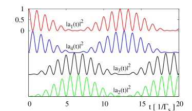
Figure 11: Time-dependent probabilities $|a_{j}(t)|^{2}$ of a transition from the initial empty configuration to the state $\left|j\right>$ defined in the basis $\left|n_{1\uparrow},n_{1\downarrow},n_{f}\right>$ obtained for the limit $\Gamma_{N}=0$, $\lambda_{1}=4$, $\lambda_{2}=0$.

Note, that for the complete setup with both quantum dots the situation is more complicated because transitions would occur in larger basis $\left|n_{1\uparrow},n_{1\downarrow},n_{f},n_{2\uparrow}\right>$ comprising 16 possible configurations. Eight states correspond to even-parity and the other eight to odd-parity sectors. Assuming the initially empty state $\left|0,0,0,0\right>$ we can express the latter state vector by a linear combination of the eight even-parity states with the corresponding time-dependent coefficients.

Introducing the auxiliary notation $\left|1\right>=\left|0,0,0,0\right>$, $\left|2\right>=\left|1,0,0,0\right>$, $\left|3\right>=\left|0,1,0,0\right>$, $\left|4\right>=\left|1,1,0,0\right>$, $\left|5\right>=\left|0,0,1,0\right>$, $\left|6\right>=\left|1,0,1,0\right>$, $\left|7\right>=\left|0,1,1,0\right>$, $\left|8\right>=\left|1,1,1,0\right>$, $\left|9\right>=\left|0,0,0,1\right>$, $\left|10\right>=\left|1,0,0,1\right>$, $\left|11\right>=\left|0,1,0,1\right>$, $\left|12\right>=\left|1,1,0,1\right>$, $\left|13\right>=\left|0,0,1,1\right>$, $\left|14\right>=\left|1,0,1,1\right>$, $\left|15\right>=\left|0,1,1,1\right>$, $\left|16\right>=\left|1,1,1,1\right>$ we can express the time-dependent occupancies of QD₁ as

$$n_{1\uparrow}(t) = \left|a_{4}(t)\right|^{2}+\left|a_{6}(t)\right|^{2}+\left|a_{10}(t)\right|^{2}+\left|a_{16}(t)\right|^{2},$$ (70)

$$n_{1\downarrow}(t) = \left|a_{4}(t)\right|^{2}+\left|a_{7}(t)\right|^{2}+\left|a_{11}(t)\right|^{2}+\left|a_{16}(t)\right|^{2}.$$ (71)

The spin-$\uparrow$ (spin-$\downarrow$) occupancy of QD₁ indicates that at a given instant of time the system can be found in configurations with the occupied second quantum dot $\left|1,0,0,1\right>$ and $\left|1,1,1,1\right>$ ($\left|0,1,0,1\right>$ and $\left|1,1,1,1\right>$).

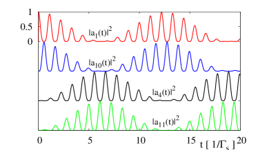
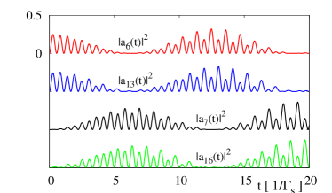
Figure 12: Time-dependent probabilities $|a_{j}(t)|^{2}$ of a transition from the initial empty configuration to the state $\left|j\right>$ defined in the basis $\left|n_{1\uparrow},n_{1\downarrow},n_{f},n_{2\uparrow}\right>$ obtained for $\Gamma_{N}=0$, $\lambda_{2}=\lambda_{1}=4$.

In Figure 12 we plot the probabilities $|a_{j}(t)|^{2}$ for the corresponding states $\left|j\right>$, as indicated. During the time evolution we observe clear oscillations between $\left|0,0,0,0\right>$ and $\left|1,0,0,1\right>$ states (two upper curves in upper panel in Fig. 12) and simultaneously oscillations between the states $\left|1,1,0,0\right>$ and $\left|0,1,0,1\right>$ (two lower curves in upper panel in Fig. 12).

From such consideration we can also determine the pairing functions, expressing them by the complex coefficients $a_{j}(t)$. For the initial empty configuration the on-dot pairing (32) takes the following form

$$C_{11}(t)=a_{1}^{\star}(t)a_{4}(t)+a_{13}^{\star}(t)a_{16}(t),$$ (72)

wheras for the initially odd-parity one obtains

$$C_{11}(t)=a_{9}^{\star}(t)a_{12}(t)+a_{5}^{\star}(t)a_{8}(t).$$ (73)

In other words, the on-dot pairing function depends on the amplitude probabilities that the system evolving over all basis states can be found in states $\left|0,0,0,0\right>$, $\left|1,1,0,0\right>$, $\left|0,0,1,1\right>$ and $\left|1,1,1,1\right>$, respectively.

Similarly, we can determine the non-local pairing functions. For the initial empty configurations they are given by

$$C_{12}(t) = a_{6}^{\star}(t)a_{16}(t)-a_{1}^{\star}(t)a_{11}(t)$$ (74)

$$C_{2f}(t) = a_{4}^{\star}(t)a_{16}(t)+a_{1}^{\star}(t)a_{13}(t).$$ (75)

Note, that (72,75) depend on the same coefficients $a_{j}(t)$, but in different combinations.

References

- Kitaev [2001] A. Yu. Kitaev, “Unpaired Majorana fermions in quantum wires,” Physics-Uspekhi 44, 131 (2001).
- Read and Green [2000] N. Read and D. Green, “Paired states of fermions in two dimensions with breaking of parity and time-reversal symmetries and the fractional quantum Hall effect,” Phys. Rev. B 61, 10267–10297 (2000).
- Silaev and Volovik [2014] M. A. Silaev and G. E. Volovik, “Andreev-Majorana bound states in superfluids,” J. Exp. Theor. Phys. 119, 1042 (2014).
- Aguado [2017] R. Aguado, “Majorana quasiparticles in condensed matter,” Riv. Nuovo Cimento 40, 523 (2017).
- Masatoshi and Yoichi [2017] S. Masatoshi and A. Yoichi, “Topological superconductors: a review,” Rep. Prog. Phys. 80, 076501 (2017).
- Lutchyn et al. [2018] R. M. Lutchyn, E. P. A. M. Bakkers, L. P. Kouwenhoven, P. Krogstrup, C. M. Marcus, and Y. Oreg, “Majorana zero modes in superconductor–semiconductor heterostructures,” Nat. Rev. Mater. 3, 52–68 (2018).
- Prada et al. [2020] E. Prada, P. San-Jose, M.W.A. de Moor, A. Geresdi, E.J.H. Lee, J. Klinovaja, D. Loss, J. Nygård, R. Aguado, and L.P. Kouwenhoven, “From Andreev to Majorana bound states in hybrid superconductor-semiconductor nanowires,” Nat. Rev. Phys. 2, 275 (2020).
- Flensberg et al. [2021] K. Flensberg, F. von Oppen, and A. Stern, “Engineered platforms for topological superconductivity and Majorana zero modes,” Nature Rev. Materials 6, 944 (2021).
- Yazdani et al. [2023] A. Yazdani, F. von Oppen, B. I. Halperin, and A. Yacoby, “Hunting for Majoranas,” Science 380, eade0850 (2023).
- Aasen et al. [2016] D. Aasen, M. Hell, R. V. Mishmash, A. Higginbotham, J. Danon, M. Leijnse, T. S. Jespersen, J. A. Folk, C. M. Marcus, K. Flensberg, and J. Alicea, “Milestones toward Majorana-based quantum computing,” Phys. Rev. X 6, 031016 (2016).
- Dvir et al. [2023] T. Dvir, G. Wang, N. van Loo, C.X. Liu, G.P. Mazur, A. Bordin, S.L.D. Ten Haaf, J.Y. Wang, D. van Driel, F. Zatelli, X. Li, F.K. Malinowski, S. Gazibegovic, G. Badawy, E.P.A.M. Bakkers, M. Wimmer, and L.P. Kouwenhoven, “Realization of a minimal Kitaev chain in coupled quantum dots,” Nature 614, 445 (2023).
- Tewari et al. [2008] S. Tewari, C. Zhang, S. Das Sarma, C. Nayak, and D.-H. Lee, “Testable signatures of quantum nonlocality in a two-dimensional chiral -wave superconductor,” Phys. Rev. Lett. 100, 027001 (2008).
- Fu [2010] L. Fu, “Electron teleportation via Majorana bound states in a mesoscopic superconductor,” Phys. Rev. Lett. 104, 056402 (2010).
- Li and Xu [2020] X.-Q. Li and L. Xu, “Nonlocality of Majorana zero modes and teleportation: Self-consistent treatment based on the Bogoliubov–de Gennes equation,” Phys. Rev. B 101, 205401 (2020).
- Hao et al. [2022] Y. Hao, G. Zhang, D. Liu, and D. E. Liu, “Anomalous universal conductance as a hallmark of non-locality in a Majorana-hosted superconducting island,” Nature Comm. 13, 6699 (2022).
- Liu et al. [2015] D. E. Liu, M. Cheng, and R. M. Lutchyn, “Probing Majorana physics in quantum-dot shot-noise experiments,” Phys. Rev. B 91, 081405(R) (2015).
- Beenakker and Oriekhov [2020] C. W. J. Beenakker and D. O. Oriekhov, “Shot noise distinguishes Majorana fermions from vortices injected in the edge mode of a chiral p-wave superconductor,” SciPost Phys. 9, 080 (2020).
- Perrin et al. [2021] V. Perrin, M. Civelli, and P. Simon, “Identifying Majorana bound states by tunneling shot-noise tomography,” Phys. Rev. B 104, L121406 (2021).
- Smirnov [2023] S. Smirnov, “Majorana differential shot noise and its universal thermoelectric crossover,” Phys. Rev. B 107, 155416 (2023).
- Leijnse and Flensberg [2011] M. Leijnse and K. Flensberg, “Scheme to measure Majorana fermion lifetimes using a quantum dot,” Phys. Rev. B 84, 140501 (2011).
- Liu and Baranger [2011] D. E. Liu and H. U. Baranger, “Detecting a Majorana-fermion zero mode using a quantum dot,” Phys. Rev. B 84, 201308 (2011).
- Lee et al. [2013] M. Lee, J. S. Lim, and R. López, “Kondo effect in a quantum dot side-coupled to a topological superconductor,” Phys. Rev. B 87, 241402 (2013).
- Cheng et al. [2014] M. Cheng, M. Becker, B. Bauer, and R. M. Lutchyn, “Interplay between Kondo and Majorana interactions in quantum dots,” Phys. Rev. X 4, 031051 (2014).
- Vernek et al. [2014] E. Vernek, P. H. Penteado, A. C. Seridonio, and J. C. Egues, “Subtle leakage of a Majorana mode into a quantum dot,” Phys. Rev. B 89, 165314 (2014).
- Deng et al. [2016] M. T. Deng, S. Vaitiekenas, E. B. Hansen, J. Danon, M. Leijnse, K. Flensberg, J. Nygård, P. Krogstrup, and C. M. Marcus, “Majorana bound state in a coupled quantum-dot hybrid-nanowire system,” Science 354, 1557 (2016).
- Ruiz-Tijerina et al. [2015] David A. Ruiz-Tijerina, E. Vernek, Luis G. G. V. Dias da Silva, and J. C. Egues, “Interaction effects on a Majorana zero mode leaking into a quantum dot,” Phys. Rev. B 91, 115435 (2015).
- Prada et al. [2017] E. Prada, R. Aguado, and P. San-Jose, “Measuring Majorana nonlocality and spin structure with a quantum dot,” Phys. Rev. B 96, 085418 (2017).
- Hoffman et al. [2017] S. Hoffman, D. Chevallier, D. Loss, and J Klinovaja, “Spin-dependent coupling between quantum dots and topological quantum wires,” Phys. Rev. B 96, 045440 (2017).
- Ptok et al. [2017] A. Ptok, A. Kobiałka, and T. Domański, “Controlling the bound states in a quantum-dot hybrid nanowire,” Phys. Rev. B 96, 195430 (2017).
- Weymann and Wójcik [2017] I. Weymann and K. P. Wójcik, “Transport properties of a hybrid Majorana wire-quantum dot system with ferromagnetic contacts,” Phys. Rev. B 95, 155427 (2017).
- Deng et al. [2018] M.-T. Deng, S. Vaitiekėnas, E. Prada, P. San-Jose, J. Nygård, P. Krogstrup, R. Aguado, and C. M. Marcus, “Nonlocality of Majorana modes in hybrid nanowires,” Phys. Rev. B 98, 085125 (2018).
- Silva et al. [2020] J. F. Silva, L. G. G. V. Dias da Silva, and E. Vernek, “Robustness of the Kondo effect in a quantum dot coupled to Majorana zero modes,” Phys. Rev. B 101, 075428 (2020).
- Sanches et al. [2020] J. E. Sanches, L. S. Ricco, Y. Marques, W. N. Mizobata, M. de Souza, I. A. Shelykh, and A. C. Seridonio, “Majorana molecules and their spectral fingerprints,” Phys. Rev. B 102, 075128 (2020).
- Majek and Weymann [2021] P. Majek and I. Weymann, “Majorana mode leaking into a spin-charge entangled double quantum dot,” Phys. Rev. B 104, 085416 (2021).
- Majek et al. [2022] P. Majek, G. Górski, T. Domański, and I. Weymann, “Hallmarks of majorana mode leaking into a hybrid double quantum dot,” Phys. Rev. B 106, 155123 (2022).
- Diniz and Vernek [2023] G. S. Diniz and E. Vernek, “Majorana correlations in quantum impurities coupled to a topological wire,” Phys. Rev. B 107, 045121 (2023).
- Baldo et al. [2023] L. Baldo, L. G. G. V. Dias Da Silva, A. M. Black-Schaffer, and J. Cayao, “Zero-frequency supercurrent susceptibility signatures of trivial and topological zero-energy states in nanowire junctions,” Supercond. Sci. Technol. 36, 034003 (2023).
- Tuovinen [2021] R. Tuovinen, “Electron correlation effect in superconducting nanowires in and out of equilibrium,” New J. Phys. 23, 083024 (2021).
- Pandey et al. [2023] B. Pandey, N. Mohanta, and E. Dagotto, “Out-of-equilibrium Majorana zero modes in interacting Kitaev chains,” Phys. Rev. B 107, L060304 (2023).
- Bauer et al. [2018] B. Bauer, T. Karzig, R.V. Mishmash, A.E. Antipov, and J. Alicea, “Dynamics of Majorana-based qubits operated with an array of tunable gates,” SciPost Phys. 5, 004 (2018).
- Barański et al. [2021] J. Barański, M. Barańska, T. Zienkiewicz, R. Taranko, and T. Domański, “Dynamical leakage of Majorana mode into side-attached quantum dot,” Phys. Rev. B 103, 235416 (2021).
- van Beek et al. [2018] I.J. van Beek, A. Levy Yeyati, and B. Braunecker, “Nonequilibrium charge dynamics in Majorana-Josephson devices,” Phys. Rev. B 98, 224502 (2018).
- Oguri et al. [2004] A. Oguri, Y. Tanaka, and A. C. Hewson, “Quantum phase transition in a minimal model for the Kondo effect in a Josephson junction,” J. Phys. Soc. Jpn. 73, 2494–2504 (2004).
- Liu et al. [2014] J. Liu, J. Wang, and F.-C. Zhang, “Controllable nonlocal transport of Majorana fermions with the aid of two quantum dots,” Phys. Rev. B 90, 035307 (2014).
- Wrześniewski et al. [2021] K. Wrześniewski, B. Baran, R. Taranko, T. Domański, and I. Weymann, “Quench dynamics of a correlated quantum dot sandwiched between normal-metal and superconducting leads,” Phys. Rev. B 103, 155420 (2021).
- Taranko and Domański [2018] R. Taranko and T. Domański, “Buildup and transient oscillations of Andreev quasiparticles,” Phys. Rev. B 98, 075420 (2018).
- Bondyopadhaya and Roy [2019] N. Bondyopadhaya and D. Roy, “Dynamics of hybrid junctions of Majorana wires,” Phys. Rev. B 99, 214514 (2019).
- Feng et al. [2021] W. Feng, L. Qin, and X.-Q. Li, “Cross correlation mediated by Majorana island with finite charging energy,” New J. Phys. 23, 123032 (2021).
- Zienkiewicz et al. [2020] T. Zienkiewicz, J. Barański, G. Górski, and T. Domański, “Leakage of Majorana mode into correlated quantum dot nearby its singlet-doublet crossover,” J. Phys.: Condens. Matter 32, 025302 (2020).
- Górski et al. [2018] G. Górski, J. Barański, I. Weymann, and T. Domański, “Interplay between correlations and Majorana mode in proximitized quantum dot,” Sci. Rep. 8, 15717 (2018).
- Barański et al. [2017] J. Barański, A. Kobiałka, and T. Domański, “Spin-sensitive interference due to Majorana state on the interface between normal and superconducting leads,” J. Phys.: Condens. Matter 29, 075603 (2017).
- Souto et al. [2016] R. S. Souto, A. Martín-Rodero, and A. Levy Yeyati, “Andreev bound states formation and quasiparticle trapping in quench dynamics revealed by time-dependent counting statistics,” Phys. Rev. Lett. 117, 267701 (2016).
- Souto et al. [2017] R. Seoane Souto, A. Martín-Rodero, and A. Levy Yeyati, “Quench dynamics in superconducting nanojunctions: Metastability and dynamical Yang-Lee zeros,” Phys. Rev. B 96, 165444 (2017).
- Stahl and Eckstein [2021] C. Stahl and M. Eckstein, “Electronic and fluctuation dynamics following a quench to the superconducting phase,” Phys. Rev. B 103, 035116 (2021).
- Kamp and Sothmann [2021] M. Kamp and B. Sothmann, “Higgs-like amplitude dynamics in superconductor-quantum-dot hybrids,” Phys. Rev. B 103, 045414 (2021).
- Seoane Souto et al. [2021] R. Seoane Souto, A. E. Feiguin, A. Martín-Rodero, and A. Levy Yeyati, “Transient dynamics of a magnetic impurity coupled to superconducting electrodes: Exact numerics versus perturbation theory,” Phys. Rev. B 104, 214506 (2021).
- Bedow et al. [2022] J. Bedow, E. Mascot, and D. K. Morr, “Emergence and manipulation of non-equilibrium Yu-Shiba-Rusinov states,” Commun. Phys. 5, 281 (2022).
- Ortmanns et al. [2023] L.C. Ortmanns, J. Splettstoesser, and M.R. Wegewijs, “Transient transport spectroscopy of an interacting quantum dot proximized by a superconductor: Charge and heat currents after a switch,” Phys. Rev. B 108, 085426 (2023).
- Wrześniewski et al. [2022] K. Wrześniewski, I. Weymann, N. Sedlmayr, and T. Domański, “Dynamical quantum phase transitions in a mesoscopic superconducting system,” Phys. Rev. B 105, 094514 (2022).
- Seoane Souto et al. [2020] R. Seoane Souto, K. Flensberg, and M. Leijnse, “Timescales for charge transfer based operations on Majorana systems,” Phys. Rev. B 101, 081407 (2020).
- Mascot et al. [2023] E. Mascot, T. Hodge, D. Crawford, J. Bedow, D.K. Morr, and S. Rachel, “Many-body majorana braiding without an exponential Hilbert space,” Phys. Rev. Lett. 131, 176601 (2023).