Wasserstein complexity penalization priors: a new class of penalizing complexity priors

Abstract

Penalizing complexity (PC) priors is a principled framework for designing priors that reduce model complexity. PC priors penalize the Kullback-Leibler Divergence (KLD) between the distributions induced by a “simple” model and that of a more complex model. However, in many common cases, it is impossible to construct a prior in this way because the KLD is infinite. Various approximations are used to mitigate this problem, but the resulting priors then fail to follow the designed principles. We propose a new class of priors, the Wasserstein complexity penalization (WCP) priors, by replacing KLD with the Wasserstein distance in the PC prior framework. These priors avoid the infinite model distance issues and can be derived by following the principles exactly, making them more interpretable. Furthermore, principles and recipes to construct joint WCP priors for multiple parameters analytically and numerically are proposed and we show that they can be easily obtained, either numerically or analytically, for a general class of models. The methods are illustrated through several examples for which PC priors have previously been applied.

Keywords: Wasserstein distance, prior distributions, PC priors, weakly informative priors

1 Introduction

Priors are an integral part of the Bayesian inference procedure. When direct prior information is available, prior distributions are used to approximate and summarize that information. This class of priors is referred to as subjective priors (see, e.g., Robert et al. (2007, Sections 3.2 and 4.2), Berger (1985, Section 3.2)). When little prior information is available or when one does not want the results to be influenced by prior information, noninformative priors are used. There is no unified definition of noninformative priors (Box and Tiao, 1973, Section 1.3; Berger, 1985, Section 3.3.1); however, the general idea is to give no preference to any specific parameters in the parameter space. Laplace (1820) proposed to assign a uniform distribution on the parameter space with a principle called the principle of insufficient reason, which is regarded as the first noninformative prior. One of the criticisms of this prior (Robert et al., 2007, Section 3.5.1) is the lack of parameterization invariance. By letting the prior be proportional to the square root of Fisher information of the parameter, Jeffrey’s prior (Jeffreys, 1946) has the property of parameterization invariance while maintaining the idea of uniformity (Kass, 1989, Section 2.3.1; Kass and Wasserman, 1996, Section 3.5). Later, reference priors have been developed as a widely used extension of Jeffrey’s prior by formalizing what is meant by an objective prior (Bernardo, 1979; Berger and Bernardo, 1989, 1992b, 1992a). See Kass and Wasserman (1996) and Consonni et al. (2018) for surveys of objective Bayesian analysis and noninformative priors.

Weakly informative priors are meant to lie between subjective and noninformative priors. An example is the maximum entropy method (Jaynes, 1968, 1983), which is useful when partial prior information exists, such as central moments or quantiles of a prior distribution. Another example that has received much attention recently are Penalizing Complexity (PC) priors (Simpson et al., 2017). PC priors are based on four principles:

• The prior should prefer “simpler” models. This requires the concept of a “base model” and a “flexible model”. Let $M(\theta)$ be a class of models that varies with respect to a parameter $\theta$, and let $\theta_{0}$ be the parameter that induces the “simplest” model $M(\theta_{0})$, referred to as the base model. Each $M(\theta)$, for $\theta\neq\theta_{0}$, is regarded as a flexible model. The prior assigned to $\theta$ should decay with respect to the complexity of the model, which can be interpreted as that it penalizes the deviation of the flexible model away from the base model.

• As a measure of complexity, the Kullback-Leibler Divergence (KLD) (Kullback and Leibler, 1951) is used as a “distance” between a flexible model and the base model. The intuition behind this is that the KLD can measure how much information is lost if a flexible model is replaced by the base model.

• The rate for penalizing the deviation should be constant. That is, if $D$ is the distance between the base model and the flexible model, then the prior density $\pi_{D}$ on $D$ satisfies $\pi_{D}(D+\delta)=r^{\delta}\pi_{D}(D)$ for any $D,\delta>0$ and some decay rate $r\in(0,1)$. This implies that the prior in $D$ is $\pi_{D}(D)=\eta\exp(-\eta D)$, where $\eta$ and $r$ are related via $r=\exp(-\eta)$. Given $\pi_{D}$, a change of variables is used to obtain the prior for the parameter of interest.

• The parameter $\eta$ (or the decay-rate $r$) is a user-specified parameter, which controls how informative the prior is, and which is set based on prior information.

These principles allow for systematically constructing priors that avoid overfitting. The strategy has been shown to provide priors with good properties in several scenarios (see, e.g. Simpson et al., 2017; Sørbye and Rue, 2017; Fuglstad et al., 2019; Ventrucci and Rue, 2016; Klein and Kneib, 2016; Van Niekerk et al., 2021). However, there are several issues and difficulties in the construction that tend to be overlooked. To illustrate one of the most common issues, let us consider a simple but important example.

Example 1.

Suppose that we wish to construction a PC prior for the precision parameter $\tau=1/\sigma^{2}$ ($\sigma$ is the standard deviation) of a centered Gaussian distribution. Simpson et al. (2017) suggests $\mu_{0}=\mathcal{N}(0,1/\tau_{0})$ with $\tau_{0}=\infty$ (i.e., a Dirac measure concentrated at 0) as base model. Each $\mu=\mathcal{N}(0,1/\tau)$ with $\tau\in(0,\infty)$ is considered to be a flexible model. In this case, ${\text{KLD}(\mu||\mu_{0})=\frac{\tau_{0}}{2\tau}(1+\frac{\tau}{\tau_{0}}\text{ln}(\frac{\tau}{\tau_{0}})-\frac{\tau}{\tau_{0}})}$, which means that the KLD is infinite for any $0<\tau<\infty$. Thus we cannot penalize this ‘distance’ between the base model and the flexible model. To address this issue, Simpson et al. (2017, Appendix A.1) proposed to consider a high, but finite $\tau_{0}$, and approximate $\text{KLD}(\mu||\mu_{0})$ by $\frac{\tau_{0}}{2\tau}$. Then, the prior density of $\tau$ is ${\pi(\tau)=\frac{\lambda}{2}\tau^{-\frac{3}{2}}\exp(-\lambda\tau^{-1/2})}$, where $\lambda=\hat{\lambda}\tau_{0}^{1/2}$ with $\hat{\lambda}$ as a free parameter. As a final step, they let $\tau_{0}\rightarrow\infty$ by choosing $\lambda$ so that $\hat{\lambda}$ is kept constant. The issue is that this final step cannot be done, since it implies that $\lambda\rightarrow\infty$. By the PC prior principles, $\lambda$ should be a user-specified hyperparameter. However, any finite value of $\lambda$ implies that $\tau_{0}\neq\infty$, which means that $\lambda$ is not a free parameter. In other words, once users specify $\lambda$, they replace the base model with a model of higher complexity. Thus, the PC prior for the precision uses an approximation of the KLD and replaces the base model with a model of higher complexity, making it difficult to interpret the prior in terms of the principles.

The issue with infinite KLD is not uncommon. It will occur whenever the two measures $\mu$ and $\mu_{0}$ are not absolutely continuous, and if $\mu_{0}$ truly is a simpler model, it will rarely be absolutely continuous with respect to $\mu$. Besides the issues mentioned in the example, another issue caused by infinite KLD is that there is no single approach to handle it. As a result, one may have more than one “PC prior” for the same parameter. Yet another issue, as pointed out by Robert and Rousseau (2017), is the asymmetry of the KLD. That is for two probability measures $\mu_{1}$ and $\mu_{2}$, $\text{KLD}(\mu_{1}||\mu_{2})$ does not necessarily equal to $\text{KLD}(\mu_{2}||\mu_{1})$. This induces some vagueness in using the principle. Robert and Rousseau (2017) also stated that the extension of PC priors to the multivariate case requires more development. Indeed, even though Simpson et al. (2017, Section 6.1) proposed a general idea and some simple cases for the extension, it does not give a practical rule for how to handle a general setting. We believe that the central issue that causes these problems is the second principle, i.e., the choice of KLD as the distance.

Our goal is to propose a new type of PC priors, Wasserstein complexity penalization (WCP) priors, using a penalization based on the Wasserstein distance in the PC framework. We will show that this choice of distance solves the issues mentioned above, and the resulting priors are mathematically tractable and the stated principles are truly followed. It in particular facilitates the construction of multivariate priors in a systematic way. We will illustrate the priors through several examples and also introduce theoretically justified numerical methods to approximate the WCP priors for cases when they are difficult to derive analytically. The outline of the article is as follows. Section 2 contains a brief review of the Wasserstein distance and the introduction of the WCP priors for models with a single parameter. Section 3 introduces illustrative applications of the WCP priors to stationary auto-regressive processes and generalized Pareto distribution. Section 4 introduces the multivariate WCP priors, for models with multiple parameters, and presents concrete recipes for how to derive these priors. Section 5 presents the numerical recipes for approximating univariate and bivariate WCP priors, some numerical examples, and the theoretical convergence results, showing bounds and conditions for convergence of the approximations in the total variation distance. The paper ends with a discussion in Section 6. Further technical details, numerical illustrations, and proofs are given in five appendices.

All results in the paper are implemented in the R (R Core Team, 2023) package WCPprior publicly available at https://github.com/BearZhen/WCPprior. Specifically, the package contains the numerical recipes for approximating the WCP priors as well as R functions, stan (Stan Development Team, 2023b, a) functions and tables to be used as user-defined priors in R-INLA (Lindgren and Rue, 2015) for all presented WCP priors.

2 Wasserstein complexity penalization priors

2.1 A brief review of Wasserstein distance

The Wasserstein distance is defined as follows (Villani, 2009).

Definition 1.

Let $(\mathcal{X},d)$ be a separable and complete metric space endowed with the Borel $\sigma$-algebra $\mathcal{B}(\mathcal{X})$, $p\in[1,\infty)$, and $\mu,\nu$ be two probability measures on $\mathcal{X}$. Then the Wasserstein distance of order $p$ (Wasserstein-$p$ distance) between $\mu$ and $\nu$ is

$$W_{p}(\mu,\nu)=\left(\inf\limits_{\pi\in\Pi(\mu,\nu)}\int_{\mathcal{X\times\mathcal{X}}}d(x,y)^{p}d\pi(x,y)\right)^{1/p}.$$

Here $\Pi(\mu,\nu)$ is the collection of all probability measures on $\mathcal{X}\times\mathcal{X}$ endowed with the product $\sigma$-algebra and having $\mu,\nu$ as marginals. That is, $\pi$, a probability measure on $\mathcal{X}\times\mathcal{X}$, should satisfy: $\pi(A\times\mathcal{X})=\mu(A),$ and $\pi(\mathcal{X}\times B)=\nu(B)$ for any $A,B\in\mathcal{B}$.

It is not straightforward to compute the Wasserstein distance in general; however, for measures on $\mathbb{R}$, the following remark (proved in Irpino and Verde (2015)) can be used.

Remark 1.

Let $\mu$ and $\nu$ be two probability measures on $\mathbbm{R}$. Then

$$W_{p}^{p}(\mu,\nu)=\int_{0}^{1}|F_{\mu}^{-1}(t)-F_{\nu}^{-1}(t)|^{p}dt\quad\text{and}\quad W_{1}(\mu,\nu)=\int_{\mathbbm{R}}|F_{\mu}(x)-F_{\nu}(x)|dx,$$

where $F_{\mu}$ and $F_{\nu}$ are the distribution functions of $\mu$ and $\nu$, with corresponding pseudo-inverse $F_{i}^{-1}(t)=\inf\{x:F_{i}(x)\geq t\}$ for $i=\mu,\nu$. Further, if $m_{\mu},m_{\nu}$ are the expected values and $\sigma^{2}_{\mu},\sigma^{2}_{\nu}$ are the variances of $\mu$ and $\nu$, then $W_{2}^{2}(\mu,\nu)=(m_{\mu}-m_{\nu})^{2}+(\sigma_{\mu}-\sigma_{\nu})^{2}+2\sigma_{\mu}\sigma_{\nu}(1-\rho_{\mu,\nu})$, where ${\rho_{\mu,\nu}=\sigma_{\mu}^{-1}\sigma_{\nu}^{-1}\int_{0}^{1}(F_{\mu}^{-1}(t)-m_{\mu})(F_{\nu}^{-1}(t)-m_{\nu})dt}$.

A few things should be noted here. First, the formulas in the remark show how to compute $W_{p}(\mu,\nu)$ analytically in many cases, and if the integrals cannot be evaluated analytically, they can be approximated numerically as we will explore later. Further, the measures $\mu$ and $\nu$ can depend on several parameters, so the formulas are not restricted to be used for priors of distributions with only one parameter.

We are interested in the Wasserstein-$p$ distance on the space of probability measures with a finite $p$-th moment, denoted by $P_{p}(\mathcal{X})$. For a fixed $x_{0}\in\mathcal{X}$, $P_{p}(\mathcal{X})$ is defined as

$$P_{p}(\mathcal{X}):=\Bigl{\{}\mu\in P(\mathcal{X});\quad\int_{\mathcal{X}}d(x_{0},x)^{p}d\mu<+\infty\Bigr{\}},$$

where $P(\mathcal{X})$ denotes a space of probability measure on $\mathcal{X}$. By the triangle inequality, if
${\int_{\mathcal{X}}d(x_{0},x)^{p}d\mu<+\infty}$ with a fixed $x_{0}$, then $\int_{\mathcal{X}}d(x_{1},x)^{p}d\mu<+\infty$ for any other $x_{1}\in\mathcal{X}$. Therefore, the definition of $P_{p}(\mathcal{X})$ does not depend on the choice of $x_{0}$. Furthermore, $W_{p}$ is a distance on $P_{p}(\mathcal{X})$ (Villani, 2009, p.94). Thus, $(P_{p}(\mathcal{X}),W_{p})$ is a metric space. In particular, $W_{p}$ is finite on $P_{p}(\mathcal{X})$. If we take $\mu=\delta_{x}$, for $x\in\mathcal{X}$, i.e., $\mu$ is a Dirac measure concentrated on $x$, then $\mu\in P_{p}(\mathcal{X})$ for every $p\geq 1$. Thus, whenever $\nu\in P_{p}(\mathcal{X})$, we have that $W_{p}(\mu,\nu)<\infty$. This will be important when we derive PC priors based on Wasserstein distance since it means that we can always choose Dirac measures as base models, and we expect them to be common choices for base models as they are the “simplest” measures.

Another property of the Wasserstein distance which is of interest to us is that $W_{p}$ metrizes the weak convergence in $P_{p}(\mathcal{X})$ (Villani, 2009, Theorem 6.9). This means that a sequence of probability measures $\{\mu_{k}\}_{k}\in P_{p}(\mathcal{X})$ converges to $\mu\in P_{p}(\mathcal{X})$ with distance $W_{p}$ if and only if $\{\mu_{k}\}_{k}$ converges weakly to $\mu$ in $P_{p}(\mathcal{X})$ (Villani, 2009, Definition 6.8). In particular, following Villani (2009, Definition 6.8), convergence with respect to the Wasserstein distance $W_{p}$ is equivalent to having at the same time convergence of the $p$th moment and weak convergence in $P(\mathcal{X})$ (i.e., the usual weak convergence of measures, that induces convergence in distribution of random variables). We refer to Villani (2009, p.98-99) for several reasons to choose the Wasserstein distance to metrize weak convergence in favor of other existing alternatives.

The following proposition contains an important case in which it is easy to compute the Wassertein-$p$ distance.

Proposition 1.

Let $X:\Omega\rightarrow\mathbb{R}^{d}$ be a random variable on a probability space $(\Omega,\mathcal{F},P)$ with finite $p$th moment, $p\geq 1$. Let $\mu_{X}$ be its distribution on $\mathbb{R}^{d}$, and let $\delta_{s}$ be the Dirac measure supported on $s\in\mathbb{R}^{d}$. Then, ${W_{p}(\delta_{s},\mu_{aX+b})=\left(\mathbb{E}\lVert aX+b-s\rVert_{\mathbb{R}^{d}}^{p}\right)^{1/p}}$, for $a,b\in\mathbb{R}$. In particular, if $b=s$, then $W_{p}(\delta_{s},\mu_{aX+b})=a\left(\mathbb{E}\lVert X\rVert_{\mathbb{R}^{d}}^{p}\right)^{1/p}$.

Proof.

The only coupling between $\mu_{aX+b}$ and $\delta_{s}$ is the independent coupling. That is, the only element in $\Pi(\mu_{aX+b},\delta_{s})$ from Definition 1 is $\pi(A\times B)=\mu_{aX+b}(A)\delta_{s}(B)$ for any $A,B\in\mathcal{B}$, where $\mathcal{B}$ denotes the Borel $\sigma$-algebra on $\mathbb{R}^{d}$. Therefore, the conclusion follows directly from Definition 1. ∎

Another important special case is when $\mu$ and $\nu$ are two Gaussian measures on $\mathbbm{R}^{d}$ with mean vectors $m_{\mu},m_{\nu}$ and non-singular covariance matrices $\Sigma_{\mu},\Sigma_{\nu}$, respectively. Then, Givens and Shortt (1984, Proposition 7) shows that

$$W_{2}^{2}(\mu,\nu)=\lVert m_{\mu}-m_{\nu}\rVert_{\mathbbm{R}^{d}}+\text{tr}(\Sigma_{\mu})+\text{tr}(\Sigma_{\nu})-2\text{tr}((\Sigma_{\mu}^{1/2}\Sigma_{\nu}\Sigma_{\mu}^{1/2})^{1/2}),$$ (1)

where $\lVert\cdot\rVert_{\mathbbm{R}^{d}}$ is the Euclidean norm on $\mathbbm{R}^{d}$ and $\text{tr}(\cdot)$ denotes the trace of a matrix.

2.2 Univariate Wasserstein complexity penalization priors

Motivated by the constant rate penalization principle of the original PC prior, we first give a definition of the PC prior based on the Wasserstein distance induced by a family of probability measures indexed by a single parameter.

To introduce the priors, we need the following notation. We let $\Theta=(\theta_{-},\theta_{+})$ be an open interval and let $(\mu_{\theta})_{\theta\in\Theta}$ be a family of probability measures on $P_{p}(\mathcal{X})$. We assume that there exists a unique $\theta_{0}\in\overline{\Theta}$ corresponding to the base model, where $\overline{\Theta}$ denotes the closure of $\Theta$, and define $\Theta_{-}=(\theta_{-},\theta_{0})$ and $\Theta_{+}=(\theta_{0},\theta_{+})$. We further define $W_{-}:\Theta_{-}\to[0,c_{-}]$ as ${W_{-}(\theta)=W_{p}(\mu_{\theta},\mu_{\theta_{0}})}$, which is the restriction of the function $\theta\mapsto W_{p}(\mu_{\theta},\mu_{\theta_{0}})$ to $\Theta_{-}$. Similarly, we define $W_{+}:\Theta_{+}\to[0,c_{+}]$ as ${W_{+}(\theta)=W_{p}(\mu_{\theta},\mu_{\theta_{0}})}$. If $\Theta_{-}$ or $\Theta_{+}$ is empty, then we define $W_{-}=0$ or $W_{+}=0$, respectively. Finally, we define $W_{-}=0$ on $\Theta_{+}$ and $W_{+}=0$ on $\Theta_{-}$. Here, $c_{-},c_{+}>0$ and are allowed to be $\infty$.

To make sure that the proposed prior is well-defined, we need the following assumption.

Assumption 1.

The family $(\mu_{\theta})_{\theta\in\Theta}$ satisfies:

1. There exists a probability measure $\mu_{\theta_{0}}\in P_{p}(\mathcal{X})$ such that $\mu_{\theta_{0}}$ is the weak limit of $\mu_{\theta}$ in $P_{p}(\mathcal{X})$ as $\theta\to\theta_{0}$.

2. Both $W_{-}$ and $W_{+}$ are injective and differentiable on their respective domains.

3. If $\Theta_{-}$ is not empty, then $\lim\limits_{\theta\rightarrow\theta_{0}}W_{-}(\theta)=0$ and $\lim\limits_{\theta\rightarrow\theta_{-}}W_{-}(\theta)=c_{-}$. Similarly, if $\Theta_{+}$ is not empty, then $\lim\limits_{\theta\rightarrow\theta_{0}}W_{+}(\theta)=0$ and $\lim\limits_{\theta\rightarrow\theta_{+}}W_{+}(\theta)=c_{+}$.

We are now ready to give the definition of the WCP_p priors. We do this by following the PC prior principles and assigning a truncated exponential distribution as the prior of $W_{p}(\mu_{\theta_{0}},\mu_{\theta})$. This yields the following definition by a change of variables.

Definition 2 (WCP priors).

Suppose that $(\mu_{\theta})_{\theta\in\Theta}$ satisfies Assumption 1, then the WCP_p prior of $\theta$ for the family $(\mu_{\theta})_{\theta\in\Theta}$ has density

$$\pi(\theta)=w_{-}\frac{\eta_{-}\exp(-\eta_{-}W_{-}(\theta))}{1-\exp(-\eta_{-}c_{-})}\left|\frac{\mathrm{d}W_{-}(\theta)}{\mathrm{d}\theta}\right|+w_{+}\frac{\eta_{+}\exp(-\eta_{+}W_{+}(\theta))}{1-\exp(-\eta_{+}c_{+})}\left|\frac{\mathrm{d}W_{+}(\theta)}{\mathrm{d}\theta}\right|,$$ (2)

for $\theta\in\Theta$, where $\eta_{-},\eta_{+}>0$ are user-specified hyperparameters to control the tail mass of the prior and

$$w_{-}=\frac{1-\exp(-\eta_{-}c_{-})}{2-\exp(-\eta_{-}c_{-})-\exp(-\eta_{+}c_{+})},\quad w_{+}=\frac{1-\exp(-\eta_{+}c_{+})}{2-\exp(-\eta_{-}c_{-})-\exp(-\eta_{+}c_{+})}.$$

It is an immediate consequence of Assumption 1 that the prior is well-defined. By construction, the prior also satisfies all principles of the PC prior framework except for the second, which has been replaced by the principle that the complexity is penalized in the Wasserstein-$p$ distance. We can also note that the fourth principle has been slightly extended since the general WCP_p prior has two user-specified parameters. This is explained in the following remark.

Remark 2.

In general, the WCP_p prior has two user-defined parameters. However, when $\theta_{0}=\theta_{-}$ or $\theta_{0}=\theta_{+}$, which are the cases in which $\theta_{0}$ is one of the end points of $\Theta$, it only has one. The reason is that one of the sets $\Theta_{-}$ and $\Theta_{+}$ is empty in this case. Without loss of generality, we assume $\Theta_{-}$ is empty. Then by Definition 2, the density of the $\text{WCP}_{p}$ prior of $\theta$ is

$$\pi(\theta)=\begin{cases}\frac{\eta_{+}\exp(-\eta_{+}W_{+}(\theta))}{1-\exp(-\eta_{+}c_{+})}\left|\frac{\mathrm{d}W_{+}(\theta)}{\mathrm{d}\theta}\right|&\text{if }c_{+}<\infty,\\ \eta_{+}\exp(-\eta_{+}W_{+}(\theta))\left|\frac{\mathrm{d}W_{+}(\theta)}{\mathrm{d}\theta}\right|&\text{if }c_{+}=\infty,\end{cases}$$

for $\theta\in\Theta$. If $\theta_{0}$ is not at the boundary of the parameter space, we can naturally recover the case of having only one user-specified parameter by setting $\eta_{+}=\eta_{-}$.

An important feature of the $\text{WCP}_{p}$ priors is that they are invariant under reparameterization in the sense that the principles are still obeyed under reparameterization. More precisely, we have the following proposition, which follows directly from (2) and the chain rule.

Proposition 2.

Let $g:\Theta\to(\phi_{-},\phi_{+})$ be an invertible and differentiable function with nonvanishing derivative. Let $\phi=g(\theta)$ be a reparameterization of the model in Definition 2, i.e., consider the family $(\mu_{\phi})_{\phi\in\Phi}$, where $\Phi=(\phi_{-},\phi_{+})$. If $\pi(\theta)$ and $\pi(\phi)$ are the $\text{WCP}_{p}$ prior densities for $\theta$ and $\phi$, respectively, then $\pi(\theta)=\pi(\phi)|g^{\prime}(\theta)|$, where $\phi=g(\theta)$. Thus, the $\text{WCP}_{p}$ prior for $\phi$ can be obtained by applying the change of variables $\phi=g(\theta)$ on the $\text{WCP}_{p}$ prior of $\theta$.

Example 2.

Consider a Gaussian measure on $\mathbbm{R}$ with mean $0$ and variance $1/\tau$, as in Example 1. We choose the base model $\mu_{0}=\mathcal{N}(0,1/\tau_{0})$ with $\tau_{0}=\infty$, and each $\mu=\mathcal{N}(0,1/\tau)$ with $\tau\in\mathbbm{R}^{+}$ is regarded as a flexible model. By (1), ${W_{2}(\mu,\mu_{\tau})=\tau^{-1/2}}$. By Definition 2, the $\text{WCP}_{2}$ prior density for $\tau$ is $\pi(\tau)=\frac{1}{2}\tau^{-3/2}\eta\exp(-\eta\tau^{-1/2})$. That is, the $\text{WCP}_{2}$ prior for $\tau$ is a type-2 Gumbel distribution, and by Proposition 2, the $\text{WCP}_{2}$ prior for the standard deviation $\sigma:=\tau^{-1/2}$ is the exponential distribution. This is the same prior as the PC prior from Simpson et al. (2017, Appendix A.1) that we showed in Example 1. Thus, the PC prior has a meaningful interpretation in terms of the Wasserstein distance even though the interpretation in terms of KLD is unclear.

Example 3.

Consider the $\text{WCP}_{2}$ prior of the mean parameter, $m$, of a Gaussian distribution $\mathcal{N}(m,\sigma^{2})$ with a fixed finite variance $\sigma^{2}$. We choose $\mathcal{N}(0,\sigma^{2})$ as base model while $m\neq 0,m\in\mathbb{R}$ corresponds to a flexible model. Let $\mu_{0}$ and $\mu_{m}$ denote the Gaussian measures corresponding to the base model and the flexible models, respectively. By (1), $W_{2}(\mu_{0},\mu_{m})=|m|$. Since $W_{2}(\mu_{0},\mu_{m})$ tends to infinity as $m\rightarrow\infty$, Definition 2 gives that the $\text{WCP}_{2}$ prior density is:

$$\pi(m)=\left\{\begin{aligned} &\frac{1}{2}\eta_{+}\exp(-\eta_{+}m),&m>0\\ &\frac{1}{2}\eta_{-}\exp(\eta_{-}m),&m<0\end{aligned}\right.$$

This example provides us with a case where $\theta_{0}$ is in the interior of $\Theta$. That is, $m_{0}=0$ is in the interior of $\mathbb{R}$ in Definition 2.

In Example 2, the Wasserstein distance between the base model and the flexible model is finite, and when $\tau\rightarrow\infty$, $\mu_{\tau}$ converges weakly to $\mu$ in $P_{2}(\mathbb{R})$ as we know from Section 2.1. However, as we mentioned in Section 1, if we use the distance based on KLD, it will not be finite unless $\tau=\tau_{0}$. As previously mentioned, this issue is not rare (e.g., see Appendix A in Simpson et al. (2017), Section 3.2 in Sørbye and Rue (2017), Section 2.2 in Fuglstad et al. (2019) and Section 3 in Ventrucci and Rue (2016)). To circumvent the issue that the distance based on the KLD may go to infinity, the approach is typically to modify the base model by considering an absolutely continuous measure with respect to the Lebesgue measure, which should be “close” in some sense to the base model (even though it is very far apart from the base model if one measures the distance with the KLD). However, such modification may increase the complexity of the base model. The priors based on Wasserstein distances $W_{p}$ do not have this problem since $W_{p}$ is finite on $P_{p}(\mathcal{X})$. Furthermore, since $W_{p}$ metrizes the weak convergence of probability measures in $P_{p}(\mathcal{X})$, the interpretability is enhanced, as we can describe the shrinkage of the flexible model towards the base model precisely. Moreover, from Proposition 2, the $\text{WCP}_{p}$ priors are invariant under reparameterization.

3 Applications of WCP priors

3.1 Stationary autoregressive processes

In this section, we discuss WCP priors for weakly stationary auto-regressive processes of order 1, denoted by AR(1). A weakly stationary AR(1) process is a discrete-time stochastic process, $\{X_{t},t\in\mathbbm{N}\}$, defined by the following recursive relation:

$$\left\{\begin{aligned} X_{t}&=\phi X_{t-1}+\varepsilon_{t},\quad t=1,...,n,\\ X_{0}&\sim\mathcal{N}(0,\sigma^{2}),\end{aligned}\right.$$

where $|\phi|\leq 1$ and $\{\varepsilon_{t}\}_{t=1}^{n}$ are i.i.d Gaussian $\mathcal{N}(0,\sigma^{2}(1-\phi^{2}))$, with $\varepsilon_{t}$ being independent from $X_{0}$ for each $t\in\{1,2,...,n\}$. In this parameterization, the marginal variances of the process are independent of $\phi$ and the process is stationary even for $|\phi|=1$.

Sørbye and Rue (2017) proposed a PC prior for the parameter $\phi$. They considered a base model for $\phi$ with two cases; either $\phi_{0}=0$, which corresponds to a base model which is discrete-time white noise, or $\phi_{0}=1$, which corresponds to a base model which is constant in time. Here, we focuse on the case $\phi_{0}=1$ as a base model as a constant process is truly “simpler” than the AR(1) process. In this case, the KLD-based distance between the base model and a flexible model with $\phi<1$ is infinite (Sørbye and Rue, 2017, Section 3.2), making it necessary to use some heuristic approximation such as the one in Example 1. We will now show that this is not the case for the WCP₂ priors.

Let $\mu_{0}$ denote the Gaussian measure induced by the base model (with $\phi=1$) and $\mu_{\phi}$ be measure induced by the flexible model with $\phi\in[-1,1)$.

Proposition 3.

The $\text{WCP}_{2}$ prior density for $\phi$ of the AR(1) process, with respect to the base model $\mu_{0}$ with $\phi=1$ is given by

$${\pi(\phi)=\left|\frac{\sigma}{\sqrt{2}}\frac{(n\phi^{n}-1+\phi^{n}-n\phi)(1-\phi)+f(\phi;n)^{2}}{f(\phi;n)\sqrt{n-\frac{f(\phi;n)}{1-\phi}}(1-\phi)^{2}}\right|\frac{\eta\exp\Bigl{(}-2\eta\sigma^{2}\Bigl{(}n-\frac{f(\phi;n)}{1-\phi}\Bigr{)}\Bigr{)}}{1-\exp(-\eta c)}},$$

where ${f(\phi;n)=\sqrt{n(1-\phi^{2})-2\phi(1-\phi^{n})}}$ and $c=\sigma\bigl{(}2n-\sqrt{2}\sqrt{1-(-1)^{n}}\bigr{)}^{1/2}<\infty$.

Proof.

Let $\Sigma_{0}$ and $\Sigma$ respectively denote the covariance matrices of the base model and of the flexible model of $\{X_{t},t=1,...n\}$ with $n<\infty$. Then, $\Sigma_{0}[i,j]=\sigma^{2}$ and ${\Sigma[i,j]=\phi^{|i-j|}\sigma^{2}}$ for $i,j=1,...,n$. Therefore, by (1),

$$W_{2}^{2}(\mu,\mu_{0})=2n\sigma^{2}-2\text{tr}\{(\Sigma_{0}^{1/2}\Sigma\Sigma_{0}^{1/2})^{1/2}\}=2\sigma^{2}\Bigl{(}n-\frac{\sqrt{n(1-\phi^{2})-2\phi(1-\phi^{n})}}{1-\phi}\Bigr{)}.$$

Observe that $W_{2}(\mu,\mu_{0})$ increases as $\phi$ decreases, and that it is upper bounded by $c$ which is $\sigma\bigl{(}2n-\sqrt{2}\sqrt{1-(-1)^{n}}\bigr{)}^{1/2}<\infty$. The result follows by applying Remark 2 and simplifying. ∎

The WCP₂ prior is different from the approximate PC prior in Sørbye and Rue (2017, Section 3.2, Equation 6). In particular, the $\text{WCP}_{2}$ prior depends on the length $n$ of the AR(1) process while the approximate PC prior from does not. However, since they used a heuristic approximated KLD in their derivation, the approximate PC prior does not truly follow the PC prior principles. It is natural that the $\text{WCP}_{2}$ prior depends on $n$ since the complexity of the base model (which is constant in time) is independent of $n$, whereas the complexity of the AR(1) process increases with $n$. Thus, since the complexity is dependent on $n$, so is the prior.

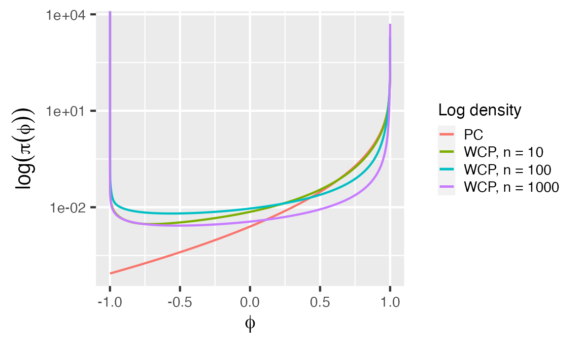
Figure 1: PC prior and $\text{WCP}_{2}$ prior densities in log scale. The user-specified hyperparameter for the PC prior is $\theta\approx 7.28$. The corresponding parameter for the $\text{WCP}_{2}$ prior is $\eta\approx 13.44$ when $n=10$, $\eta\approx 2.17$ when $n=100$, and $\eta\approx 0.57$ when $n=1000$.

A comparison between the two priors is shown in Figure 1. The user-specified hyperparameters for both priors are chosen so that the priors satisfy $P(\phi>U)=\alpha$, where $U=0.9,\alpha=0.9$ and $\sigma=0.1$. We can see that the $\text{WCP}_{2}$ prior assigns less mass near the base model $\phi=1$ than the PC prior for $n=10$, and when $n$ increases, the $\text{WCP}_{2}$ prior becomes more concentrated around the base model. To further compare the priors, we performed a simulation study that compares the Maximum A Posteriori (MAP) estimations under the $\text{WCP}_{2}$ prior, the approximate PC prior, and a uniform prior on $\phi$ with simulated data from an AR(1) process with $n=10,100,1000$. For each value of $n$, we generate data with $\phi=0.5$ and then compute the MAP estimates. This is repeated $5000$ times, and the whole procedure is then repeated with data where the true parameter is $\phi=-0.5$. Figure 2 shows box plots of the resulting estimates. Compared to the uniform prior, the MAP estimations under both the $\text{WCP}_{2}$ prior and PC prior are biased towards the base model ($\phi=1$) when $n$ is small, while when $n$ is larger, that bias disappears. This is reasonable because a small value of $n$ does not provide strong evidence to move the estimation of $\phi$ away from the base model. However, as expected from the results in Figure 1, the $\text{WCP}_{2}$ prior has a slightly lower bias for small values of $n$, even though the user-specified parameters are chosen in the same way.

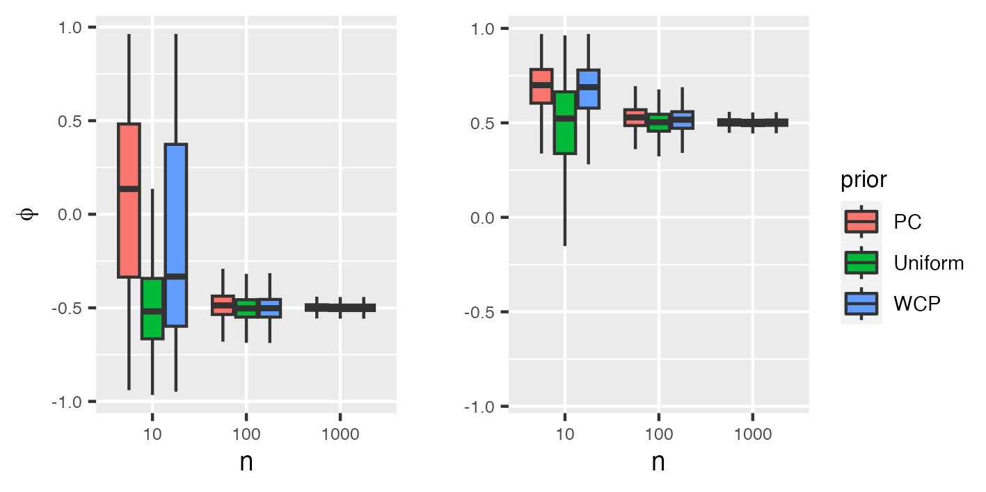
Figure 2: Distributions of MAP estimations of $\phi$ under different priors. The left figure shows the results for $\phi=-0.5$ and the right one shows the results for $\phi=0.5$

3.2 The tail index of the generalized Pareto distribution

PC priors have also been used in extreme value statistics. Specifically, Opitz et al. (2018) proposed a PC prior for the tail index of a generalized Pareto distribution with density
${f_{\xi}(y)=\sigma^{-1}(1+\xi y/\sigma)^{-1/\xi-1},y>0}$, where $\xi\in\mathbbm{R}$ is the tail index and $\sigma>0$ is a scale parameter. Opitz et al. (2018, Section 3.3) considered $\xi\in[0,1)$ specifically, since other values of $\xi$ are not realistic for modeling, and derived a KLD-based PC prior for $\xi$. In this section, we compare that PC prior with the corresponding WCP prior.

When $\xi\in[0,1)$, the generalized Pareto distribution has a finite first moment, which means that the associated probability measures belong to $P_{1}(\mathcal{X})$. Thus, the natural choice is to consider the $\text{WCP}_{1}$ prior of $\xi$. When $\xi=0$, the generalized Pareto distribution is the exponential distribution which has the lightest tail compared to other values of $\xi\in[0,1)$. Therefore, Opitz et al. (2018) chose $\xi_{0}=0$ as the parameter of the base model, with density $f_{\xi_{0}}(y)=\sigma^{-1}\text{exp}(-y/\sigma)$.

Proposition 4.

The $\text{WCP}_{1}$ prior for $\xi$ with respect to the base model induced by ${\xi=\xi_{0}=0}$, and flexible model $\xi\in(0,1)$, is given by

$$\pi(\xi)=\frac{\eta}{(1-\xi)^{2}}\exp\Bigl{(}-\eta\frac{\xi}{1-\xi}\Bigr{)},$$

where $\eta>0$ is the user-specified hyperparameter controlling the tail mass of the prior.

Proof.

Let $W_{1}(\xi)$ denote the Wasserstein-1 distance between the base model and the flexible model with parameter $\xi$. Then, $W_{1}(\xi)=\xi/(1-\xi)$ by the formula in Remark 1. The result thus follows by applying Remark 2.

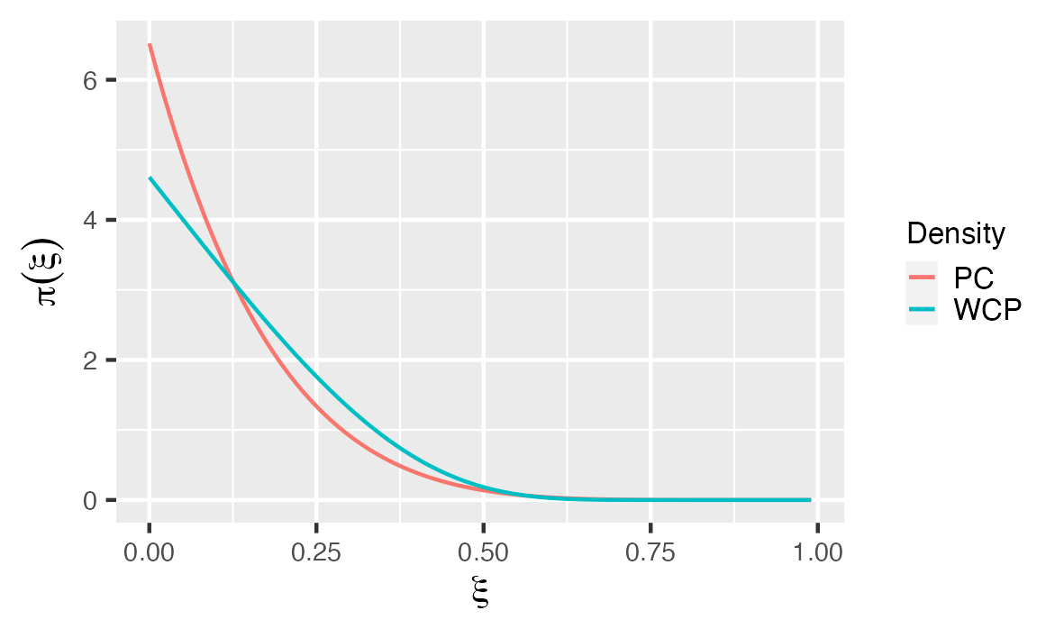
Figure 3: PC and $\text{WCP}_{1}$ prior densities of the tail index of the generalized Pareto distribution. The user-specified hyperparameter for both priors is 4.61.

∎

Figure 3 shows the PC prior from Opitz et al. (2018, eq. 8) and the $\text{WCP}_{1}$ prior. Both priors satisfy $P(\xi>U)=\alpha$, for $U=0.5,\alpha=0.01$. The PC prior concentrates more than the $\text{WCP}_{1}$ prior around the base model, which means that it has a higher penalization.

4 Multivariate WCP priors

In this section, we extend the WCP priors to models with multiple parameters. We begin with the general setup, then provide some specific examples for models with two parameters, and finally compare the multivariate priors to the two-step approach that is commonly used within the PC prior framework.

4.1 General setup

Suppose that we have a model $\mu_{\boldsymbol{\theta}}$ with $d$ real-valued parameters $\boldsymbol{\theta}=[\theta_{1},...,\theta_{d}]\in\mathbb{R}^{d}$ which we want to assign a joint prior distribution for. We assume that the parameter domain is $\boldsymbol{\Theta}=\prod_{i=1}^{d}\Theta_{i}$, where each $\Theta_{i}$ is an open interval, $i=1,\ldots,d$ and further assume that the probability measures $(\mu_{\boldsymbol{\theta}})_{\boldsymbol{\theta}\in\boldsymbol{\Theta}}$ belong to $P_{p}(\mathcal{X})$. Further, suppose that the base model has parameter vector $\boldsymbol{\theta}_{0}\in\overline{\boldsymbol{\Theta}}\setminus\boldsymbol{\Theta}$, where $\overline{\boldsymbol{\Theta}}$ denotes the closure of $\boldsymbol{\Theta}$. Let $W_{p}(\boldsymbol{\theta})=W_{p}(\mu_{\boldsymbol{\theta}_{0}},\mu_{\boldsymbol{\theta}})$ denote the Wasserstein-$p$ distance between the base model $\mu_{\boldsymbol{\theta}_{0}}$ and a flexible model $\mu_{\boldsymbol{\theta}}$ and define $\sup_{\boldsymbol{\theta}\in\boldsymbol{\Theta}}W_{p}(\boldsymbol{\theta})=c$, where $c$ can be infinity. In addition, we make the following assumption.

Assumption 2.

The family $(\mu_{\boldsymbol{\theta}})_{\boldsymbol{\theta}\in\boldsymbol{\Theta}}$ satisfies:

1. $\mu_{\boldsymbol{\theta}_{0}}$ is the weak limit of $\mu_{\boldsymbol{\theta}}$ in $P_{p}(\mathcal{X})$ as $\boldsymbol{\theta}\to\boldsymbol{\theta}_{0}$ in $\mathbb{R}^{d}$.

2. $\boldsymbol{\theta}\mapsto W_{p}(\boldsymbol{\theta})$ is of class $C^{1}$ on $\boldsymbol{\Theta}$.

3. $W_{p}(\boldsymbol{\theta})$ has a nonvanishing gradient for $\boldsymbol{\theta}\neq\boldsymbol{\theta}_{0}$.

Assumption 2:(2)-(3) mean that $W_{p}(\cdot)$ is a submersion, which is both realistic and natural, since it says that there is no critical point for the Wasserstein distance among the flexible models, which is reasonable for any meaningful parameterization of the model.

Remark 3.

Assumption 2:(1) gives that $W_{p}(\mu_{\boldsymbol{\theta}_{0}},\mu_{\boldsymbol{\theta}})\rightarrow 0$ as $\lVert\boldsymbol{\theta}_{0}-\boldsymbol{\theta}\rVert_{\mathbb{R}^{d}}\rightarrow 0$. For a constant $w>0$, let $S_{w}=\{\boldsymbol{\theta}|W_{p}(\boldsymbol{\theta})=w\}$ be the level set of $W_{p}(\boldsymbol{\theta})$ corresponding to $w$. Assumption 2:(2)-(3) and the inverse function theorem imply that $S_{w}$ is a $C^{1}$-hypersurface in $\mathbb{R}^{d}$. It also implies that $\boldsymbol{\Theta}$ is a foliation formed by the level sets $S_{w}$.

We define multivariate WCP priors by assigning a (truncated) exponential distribution to the values of the Wasserstein distance $w$, while independently, assigning uniform distributions over each level set $S_{w}$. That is, we penalize the complexity in $w$ but make no difference between models with the same $W_{p}(\boldsymbol{\theta})$. Simpson et al. (2017, Section 6.1) proposed a similar idea with the KLD. There, they derived multivariate PC priors for a restricted class of models that have very specific forms of the KLD (see Simpson et al. (2017, Equations (6.3) and (6.4))). No examples of multivariate PC priors were presented for more general forms of KLD. However, it is not common to find Wasserstein distances that satisfy the requirements in Simpson et al. (2017, Section 6.1) under natural parameterization of models. Instead of only considering specific cases, we propose the following concrete recipe for deriving the multivariate WCP priors in a general setting.

Definition 3 (Multivariate WCP priors).

Let Assumption 2 hold. Also assume that for every $w>0$ with $S_{w}\neq\emptyset$ there exists an area-preserving parameterization of $S_{w}$ given by $\gamma_{w}:U_{w}\rightarrow S_{w}$. Further, assume that $U_{w}=\prod_{i=1}^{d-1}U_{i,w}$, where $U_{i,w}\subset\mathbb{R}$ are open intervals, ${i=1,...,d-1}$. Now, let $\{u_{i,w}\}_{i=1}^{d-1}$ denote the parameters of $S_{w}$ under this parameterization. Then, the joint WCP prior density of $w$ and $\{u_{i,w}\}_{i=1}^{d-1}$ is:

$$\pi_{w,\{u_{i,w}\}_{i=1}^{d-1}}(w,u_{1,w},...,u_{d-1,w})=\frac{\eta\exp(-\eta w)}{1-\exp(-\eta c)}\prod_{i=1}^{d-1}\frac{\mathbbm{1}_{u_{i,w}\in U_{i,w}}}{\lambda(U_{i,w})},$$

where $\lambda(\cdot)$ is the Lebesgue measure on $\mathbb{R}$ and ${c:=\sup_{\boldsymbol{\theta}\in\boldsymbol{\Theta}}W_{p}(\boldsymbol{\theta})}$. By a change of variables, the multivariate $\text{WCP}_{p}$ prior density for $\boldsymbol{\theta}$ is:

$$\pi(\boldsymbol{\theta})=|\det J_{W_{p},\{u_{i,W_{p}(\boldsymbol{\theta})}\}_{i=1}^{d-1}}(\boldsymbol{\theta})|\frac{\eta\exp(-\eta W_{p}(\boldsymbol{\theta}))}{1-\exp(-\eta c)}\prod_{i=1}^{d-1}\frac{\mathbbm{1}_{u_{i,W_{p}(\boldsymbol{\theta})}\in U_{i,W_{p}(\boldsymbol{\theta})}}}{\lambda(U_{i,W_{p}(\boldsymbol{\theta})})},$$ (3)

where $J_{W_{p},\{u_{i,W_{p}(\boldsymbol{\theta})}\}_{i=1}^{d-1}}(\boldsymbol{\theta})$ denotes the Jacobian of $W_{p}(\boldsymbol{\theta}),\{u_{i,W_{p}(\boldsymbol{\theta})}\}_{i=1}^{d-1}$ evaluated at $\boldsymbol{\theta}$ and $\eta>0$ is a user-specified hyperparameter.

An area-preserving parameterization means that for any two sets $A,B\subset U_{w}$, if we have $\lambda_{U_{w}}(A)=\lambda_{U_{w}}(B)$, then $\lambda_{S_{w}}(\gamma(A))=\lambda_{S_{w}}(\gamma(B))$, where $\lambda_{U_{w}}$ denotes the Lebesgue measure on $U_{w}$ and $\lambda_{S_{w}}$ denotes the surface measure on $S_{w}$, that is, $\lambda_{S_{w}}(A)$ is the surface area of $A$, where $A$ is a Borel subset of $S_{w}$. Thus, for fixed $w$, if $u$ follows a uniform distribution on $U_{w}$, then $\gamma_{w}(u)$ follows a uniform distribution on $S_{w}$.

The multivariate WCP priors also satisfy the invariance under the parameterization in the same sense as in Proposition 2. The following result follows directly from the chain rule together with Definition 3.

Proposition 5.

Let the assumptions of Definition 3 hold. Let, also, $g:\boldsymbol{\Theta}\to\boldsymbol{\Phi}$ be a diffeomorphism. Let $\boldsymbol{\phi}=g(\boldsymbol{\theta})$ be a reparameterization of the model in Definition 2. Let $\pi(\boldsymbol{\theta})$ and $\pi(\boldsymbol{\phi})$ be the multivariate $\text{WCP}_{p}$ priors to $\theta$ and $\phi$, respectively. Then,

$$\pi(\boldsymbol{\theta})=\pi(\boldsymbol{\phi})|\det J_{g}(\boldsymbol{\theta})|,$$

where $\boldsymbol{\phi}=g(\boldsymbol{\theta})$ and $J_{g}(\boldsymbol{\theta})$ denotes the Jacobian of $g$ evaluated at $\boldsymbol{\theta}$. That is, the multivariate $\text{WCP}_{p}$ prior density for $\boldsymbol{\phi}$ can be obtained by applying the change of variables $\boldsymbol{\phi}=g(\boldsymbol{\theta})$ on the multivariate $\text{WCP}_{p}$ prior density of $\boldsymbol{\theta}$.

4.2 Bivariate WCP priors

For models with two parameters, the level set in the Definition 3 is a level curve and $\boldsymbol{\Theta}\subset\mathbb{R}^{2}$. We can create a Cartesian coordinate system for the two parameters, $\theta_{1}$ and $\theta_{2}$, with each one representing one axis. The two parameters corresponding to a base model should be a point in that coordinate system. Without loss of generality, we can choose a parameterization so that the point is the origin of the coordinate system. Let $w=W_{p}(\theta_{1},\theta_{2})$ be the Wasserstein distance between a flexible model with parameters at $(\theta_{1},\theta_{2})$ and the base model. Definition 3 requires us to assign uniform distributions over each level curve and a (truncated) exponential distribution on the Wasserstein distance. An area-preserving parameterization in this case means a parameterization of the level curve by arc-length.

Example 4.

Let us derive the bivariate $\text{WCP}_{2}$ prior for the mean $m\in\mathbb{R}$ and the standard deviation $\sigma\in\mathbb{R}^{+}$ of a Gaussian distribution. A natural choice for the parameters of the base model is $m_{0}=0,\sigma_{0}=0$ since it induces a Dirac measure concentrated at $(0,0)$ in $\mathbb{R}^{2}$. By (1), the Wasserstein-2 distance between the base model and a flexible model with mean $m$ and standard deviation $\sigma$ is $W_{2}(m,\sigma)=(m^{2}+\sigma^{2})^{1/2}$, which coincides with the Euclidean distance on $\mathbb{R}\times(0,\infty)$. For any fixed value of $W_{2}(m,\sigma)=w>0$, the level curve $S_{w}$ is a semi-circle with radius $w$. A parameterization of $S_{w}$ by arc-length is $\gamma(\varphi)=(w\cos(\varphi),w\sin(\varphi))$, where $\varphi\in(0,\pi)$ denotes the polar angle. By assigning an exponential distribution to $w$ and a uniform distribution to $\varphi$, the joint $\text{WCP}_{2}$ prior of $W_{2}(m,\sigma)$ and $\varphi$ is:

$$\pi_{w,\varphi}(w,\varphi)=\eta\exp(-\eta w)\frac{\mathbbm{1}_{\varphi\in(0,\pi)}}{\pi}.$$

Note that $\varphi=\arccos(\frac{m}{W(m,\sigma)})$ so, by (3), the $\text{WCP}_{2}$ prior of $(m,\sigma)$ is:

$$\pi(m,\sigma)=\frac{1}{(m^{2}+\sigma^{2})^{1/2}}\eta\exp(-\eta(m^{2}+\sigma^{2})^{1/2})\frac{\mathbbm{1}_{\arccos(\frac{m}{(m^{2}+\sigma^{2})^{1/2}})\in(0,\pi)}}{\pi}.$$ (4)

In general, it is difficult to find a parameterization by arc-length of level curves. The following recipe provides a solution for how to derive the WCP_p priors for the case in which each level curve is a graph of a function.

Recipe 1.

Suppose that for each $w>0$, the level curve $S_{w}$ is a graph of a function. In particular, by exchanging the order of $\theta_{1}$ and $\theta_{2}$ if necessary, it can be parameterized as
$\alpha(\theta_{1},\theta_{2};w)=(\theta_{1},f(\theta_{1};w))$, where $f(\cdot;w)$ is a function of $\theta_{1}$ that depends on the Wasserstein distance $w$. Let $(\theta_{1}^{o},\theta_{1}^{e})$ denote the domain of $\theta_{1}$ and $s=u_{1}(\theta_{1};w)$ denote the arc length from $(\theta_{1}^{o},f(\theta_{1}^{o};w))$ to $(\theta_{1},f(\theta_{1};w))$. Recall that $c:=\sup_{\boldsymbol{\theta}\in\boldsymbol{\Theta}}W_{p}(\boldsymbol{\theta})$. The steps to derive the bivariate WCP_p prior are:

1. Compute $u_{1}(\theta_{1};w)$ and the total arc length $l(w)$ as

   $$u_{1}(\theta_{1};w)=\int_{\theta_{1}^{o}}^{\theta_{1}}\sqrt{1+\left({\mathrm{d}f(x;w)}/{\mathrm{d}x}\right)^{2}}\mathrm{d}x,\quad l(w)=\int_{\theta_{1}^{o}}^{\theta_{1}^{e}}\sqrt{1+\left({\mathrm{d}f(x;w)}/{\mathrm{d}x}\right)^{2}}\mathrm{d}x.$$

2. Compute the Jacobian determinant

   $$\det J_{W_{p},u_{1}}(\theta_{1},\theta_{2})=\left|\begin{array}[]{cc}\frac{\partial W_{p}(\theta_{1},\theta_{2})}{\partial\theta_{1}}&\frac{\partial W_{p}(\theta_{1},\theta_{2})}{\partial\theta_{2}}\\ \frac{\partial u_{1}(\theta_{1};W_{p}(\theta_{1},\theta_{2}))}{\partial\theta_{1}}&\frac{\partial u_{1}(\theta_{1};W_{p}(\theta_{1},\theta_{2}))}{\partial\theta_{2}}\end{array}\right|.$$ (5)

3. Compute the density of the bivariate WCP prior of $(\theta_{1},\theta_{2})$ as

   $$\pi_{\theta_{1},\theta_{2}}(\theta_{1},\theta_{2})=|\det J_{W_{p},u_{1}}(\theta_{1},\theta_{2})|\frac{\eta\exp(-\eta W_{p}(\theta_{1},\theta_{2}))}{1-\exp(-\eta c)}\frac{1}{l(W_{p}(\theta_{1},\theta_{2}))},\quad(\theta_{1},\theta_{2})\in\boldsymbol{\Theta}.$$ (6)

It can be noted that a parameterization by arc-length is $\gamma(s)=\alpha\circ u_{1}^{-1}(s)$. This might be difficult to compute because it involves the inversion of $u_{1}$, but this inversion is not needed in order to compute the WCP prior through the recipe. It is easy to verify that by following the recipe for the mean $m$ and standard deviation $\sigma$ of a Gaussian distribution, one arrives as the $\text{WCP}_{2}$ in Example 4. The recipe was not needed there since it was easy to obtain the parameterization by arc length. Example 5 shows an application where the recipe greatly simplifies the computation. Before that, we have the following result showing the expression of the WCP prior for regions that are not necessarily of the form $I\times J$, where $I$ and $J$ are intervals.

Proposition 6.

Let $\hat{\boldsymbol{\Theta}}\subset\mathbb{R}^{2}$ be a region such that there exists an invertible $C^{1}$ function ${\Psi:\hat{\boldsymbol{\Theta}}\to\boldsymbol{\Theta}}$, where $\boldsymbol{\Theta}=I\times J$, with $I$ and $J$ being intervals, and let $\hat{W}_{p}:\hat{\boldsymbol{\Theta}}\to\mathbb{R}$ be a Wasserstein distance defined on $\hat{\boldsymbol{\Theta}}$ with respect to a base model $\hat{\boldsymbol{\theta}}_{0}$. Also, we let $W_{p}(\boldsymbol{\theta})=\hat{W}_{p}(\Psi^{-1}(\boldsymbol{\theta}))$, and $\boldsymbol{\theta}=(\theta_{1},\theta_{2})=\Psi(\hat{\theta}_{1},\hat{\theta}_{2})$, for $\hat{\boldsymbol{\theta}}=(\hat{\theta}_{1},\hat{\theta}_{2})\in\hat{\boldsymbol{\Theta}}$. Suppose that Assumption 2 holds for $\boldsymbol{\theta}\to W_{p}(\boldsymbol{\theta})$ and that the assumptions in Recipe 1 hold for $\boldsymbol{\theta}$ and $W_{p}(\cdot)$. Then, the WCP_p prior for $\hat{\boldsymbol{\theta}}$ is

$$\pi_{\hat{\theta}_{1},\hat{\theta}_{2}}(\hat{\theta}_{1},\hat{\theta}_{2})=|\det J_{\Psi}(\hat{\theta}_{1},\hat{\theta}_{2})|\pi_{\theta_{1},\theta_{2}}(\theta_{1},\theta_{2}),$$

where $J_{\Psi}(\cdot)$ is the Jacobian of $\Psi(\cdot)$. In particular, one can also use Recipe 1 if the parameter domain is a conic region $\{(x,y)\in\mathbb{R}^{2}:(x,y)=(r\cos(\theta),r\sin(\theta)),r>0,\theta\in[0,\phi]\},$ $\phi\in(0,\pi/2).$

Proof.

The result follows directly from the change of variables formula, together with an application of Sard’s theorem to drop the requirement that $\det J_{\Psi}(\cdot)\neq 0$ (e.g., Spivak, 1965, p.72). For the conic region, one can simply consider the map $\Psi(x,y)=r(\cos(\alpha\theta),\sin(\alpha\theta))$, where $(r,\theta)=\Phi(x,y)=(\sqrt{x^{2}+y^{2}},\text{arccos}(x/\sqrt{x^{2}+y^{2}})$ and $\alpha=\pi/(2\phi)$. ∎

We have the following corollary whose proof is immediate:

Corollary 1.

Let $\hat{\boldsymbol{\Theta}}=\hat{\boldsymbol{\Theta}}_{1}\cup\cdots\cup\hat{\boldsymbol{\Theta}}_{k}\subset\mathbb{R}^{2}$, where $k\in\mathbb{N}$. Further, assume that for each $k$, $\hat{\boldsymbol{\Theta}}_{k}$ satisfies the assumptions of Proposition 6, for some function $\Phi_{k}(\cdot)$. Finally, assume that for each $i\neq j$, $\lambda(\hat{\boldsymbol{\Theta}}_{i}\cap\hat{\boldsymbol{\Theta}}_{j})=0$, where $\lambda(\cdot)$ is the Lebesgue measure and $i,j=1,\ldots,k$. Then,

$$\pi_{\hat{\theta}_{1},\hat{\theta}_{2}}(\hat{\theta}_{1},\hat{\theta}_{2})=\sum_{j=1}^{k}|\det J_{\Psi_{j}}(\hat{\theta}_{1},\hat{\theta}_{2})|\pi_{\Psi_{j}(\hat{\theta}_{1},\hat{\theta}_{2})}(\Psi_{j}(\hat{\theta}_{1},\hat{\theta}_{2}))1_{(\hat{\theta}_{1},\hat{\theta}_{2})\in\Psi_{j}^{-1}(\boldsymbol{\Theta}_{k})}.$$

In particular, one can also apply Recipe 1 for more general conic regions such as the following: $\{(x,y)\in\mathbb{R}^{2}:(x,y)=(r\cos(\theta),r\sin(\theta)),r>0,\theta\in[0,\phi]\},$ $\phi\in(0,2\pi).$

Example 5.

In Section 3.2, we considered a $\text{WCP}_{1}$ prior for the tail index of the generalized Pareto distribution. We now derive the two-dimensional $\text{WCP}_{1}$ prior for $\xi$ and $\sigma$ of the generalized Pareto distribution. We select $\xi_{0}=0,\sigma_{0}=0$ as the parameters for the base model since they induce a Dirac measure on $\mathbb{R}$ centered at $0$. We let the flexible models be $\xi\in[0,1),\sigma\in(0,+\infty)$. The generalized Pareto density $f_{\xi,\sigma}(y)$ generates a scale family where the scale parameter is $\sigma$. According to Proposition 1, the Wasserstein-1 distance between the base model and a flexible model is $W_{1}(\xi,\sigma)=\sigma\mathbb{E}X=\frac{\sigma}{1-\xi}$ where $X$ follows a generalized Pareto distribution with $\sigma=1$. By fixing $W_{1}(\xi,\sigma)$ to a positive value $w$, we obtain a level curve that can be parameterized by $\alpha(\sigma)=(\sigma,1-\frac{\sigma}{w})$, which is a straight line in the Cartesian coordinate system. By following Recipe 1, let $s=u_{1}(\sigma;w)$ denote the partial arc length of the level curve from the point $(0,1)$ to $(\sigma,1-\frac{\sigma}{w})$ as a function of $\sigma$. We have that $u_{1}(\sigma;w)=\frac{\sigma}{w}{\sqrt{w^{2}+1}}$. Therefore, the full arc length of the level curve is $l(w)=\sqrt{w^{2}+1}$. By Recipe 1:(3), we obtain the $\text{WCP}_{1}$ prior of $(\xi,\sigma)$ as

$$\pi_{\sigma,\xi}(\sigma,\xi)=\frac{\sqrt{(1-\xi)^{2}+\sigma^{2}}}{(1-\xi)^{2}}\pi_{w,s}(\frac{\sigma}{1-\xi},\sqrt{(1-\xi)^{2}+\sigma^{2}})=\frac{\eta}{1-\xi}\exp(-\eta\frac{\sigma}{1-\xi}).$$ (7)

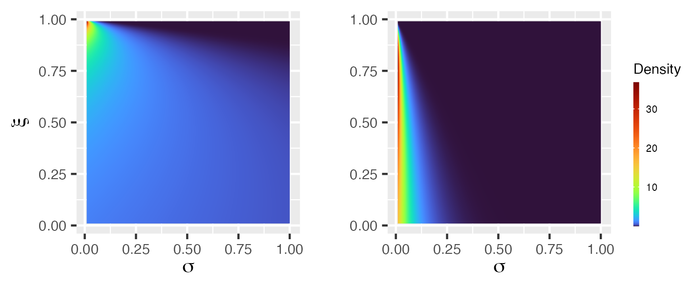
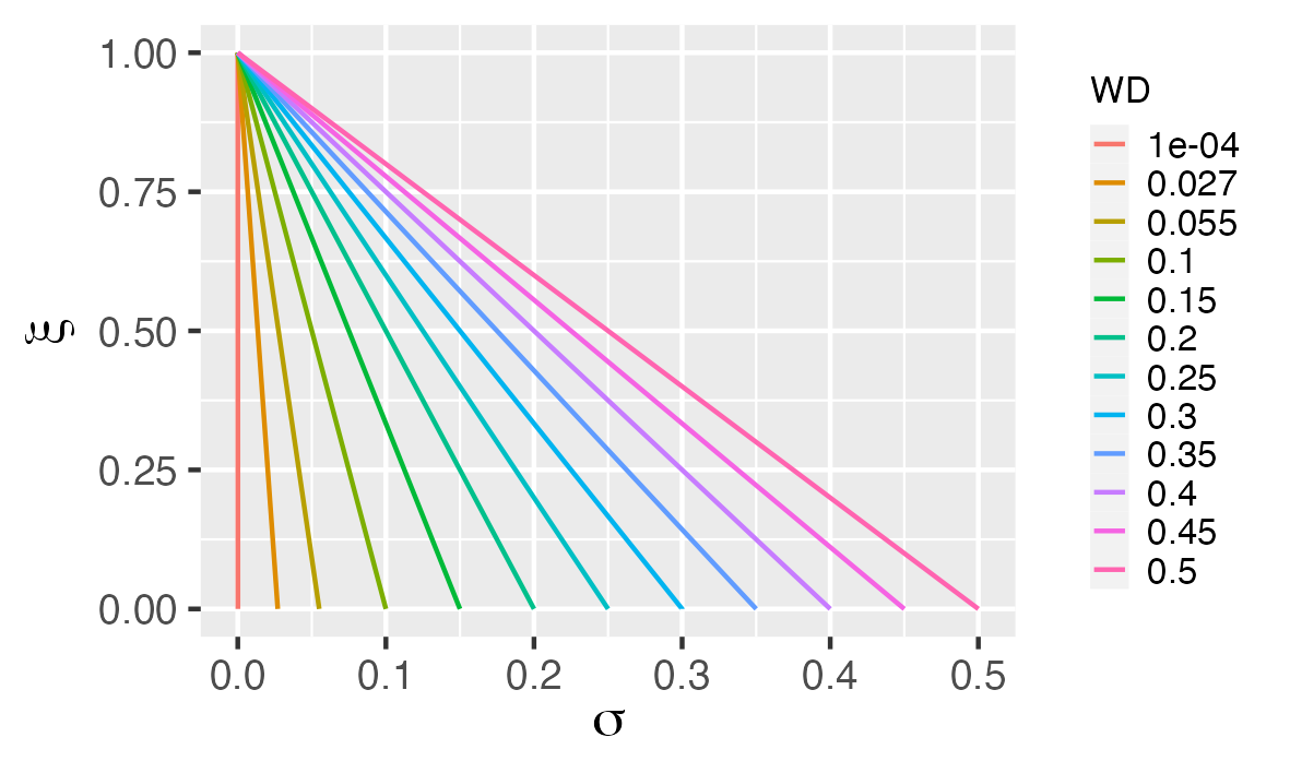
Figure 4: $\text{WCP}_{1}$ prior density of $\xi$ and $\sigma$ with $\eta=1$ (left) and $\eta=20$ (middle). The right panel shows level curves of the Wasserstein–1 distance (WD).

Figure 4 shows two examples of the WCP₁ densities of $(\sigma,\xi)$ for the generalized Pareto distribution, when $\eta=1,20$. The prior with $\eta=1$ concentrates near $\xi=1$ and $\sigma=0$. This may seem counter-intuitive since the base model for one-dimensional $\text{WCP}_{1}$ prior of $\xi$ is $\xi=0$. To explain this, consider the right panel of Figure 4 which shows some level curves of the Wasserstein distance. We note, from Figure 4, that when $\eta=20$ the prior concentrates near the Y-axis. In this case, the exponential law of the Wasserstein distance assigns negligible probability for “large” values of the Wasserstein distance, thus concentrating the density near parameters whose Wasserstein distances have small values. On the other hand, when $\eta=1$, the exponential distribution allows values of the Wasserstein distance to be larger with a higher probability. For a fixed Wasserstein distance that is not very small, the value of $\sigma$ is relatively sensitive to the value of $\xi$. This means that if $\xi$ is close to 1, $\sigma$ will necessarily be near 0 but when $\xi$ is away from 1, $\sigma$ can vary more. Since uniform distributions are assigned over each level curve this explains the concentration behavior.

4.3 A comparison with the two-step approach

Fuglstad et al. (2019, Section 2.2) proposed a way to derive a joint PC prior of two parameters, which is commonly used in practice which we will refer to as the two-step approach. In this section, we will formalize a counterpart of this idea for WCP priors and compare it with the one in Definition 3. Suppose that we have two parameters $\theta_{1}$ and $\theta_{2}$. Let $\theta_{1}=\theta_{1,0},\theta_{2}=\theta_{2,0}$ be the values that correspond to the base model. The first step of this approach is to derive a WCP prior for one of the parameters, say $\theta_{1}$, while fixing $\theta_{2}=\theta_{2,0}$. This prior distribution is a conditional distribution of $\theta_{1}$ given that $\theta_{2}=\theta_{2,0}$. However, in the two steps approach, this is treated as a prior of $\theta_{1}$, and is denoted by $\pi(\theta_{1})$. The second step is to derive the conditional WCP prior $\pi(\theta_{2}|\theta_{1})$ for $\theta_{2}$ given $\theta_{1}$. The two-step WCP prior density is then $\pi(\theta_{1})\pi(\theta_{2}|\theta_{1})$.

Example 6.

Let us derive the two-step approach prior for the mean $m$ and the standard deviation $\sigma$ of a Gaussian distribution. We derive the $\text{WCP}_{2}$ prior for $m$ with $\sigma=0$ first. The Wasserstein-2 distance between $\mathcal{N}(m,0)$ and $\mathcal{N}(0,0)$ is $W_{2}(\mathcal{N}(m,0),\mathcal{N}(0,0))=|m|$, thus $\pi(m|\sigma=0)=\eta_{1}\exp(-\eta_{1}|m|)$ for $m\neq 0$, where $\eta_{1}$ is a user-specified hyperparameter. Next, we derive the $\text{WCP}_{2}$ prior for $\sigma|m$. We have that $W_{2}(\mathcal{N}(m,\sigma),\mathcal{N}(m,0))=\sigma$. Therefore, $\pi(\sigma|m)=\eta_{2}\exp(-\eta_{2}\sigma)$ for $\sigma>0$, where $\eta_{2}$ is a user-specified hyperparameter. Combining the two steps yields the two-step prior

$$\pi(m,\sigma)=\frac{1}{2}\eta_{1}\eta_{2}\exp(-\eta_{1}|m|-\eta_{2}\sigma).$$

Figure 5 contains a comparison between the $\text{WCP}_{2}$ prior from (4) and the two-step prior. We can note that the two priors behave very differently near the base model.

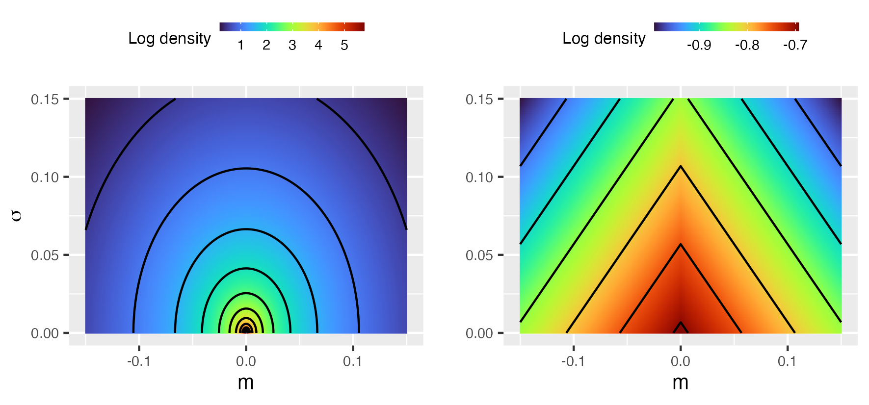
Figure 5: $\text{WCP}_{2}$ prior (left) with $\eta=1$ and two-step approach prior (right) with $\eta_{1}=\eta_{2}=1$ for $m$ and $\sigma$ for the normal distribution, with contour lines in black.

It should be noted that he order of the parameters in which the two steps are performed may affect the final result for the two-step prior. This was not the case for Example 6, whereas the order matters in the following example.

Example 7.

Let us derive the two-steps $\text{WCP}_{1}$ prior for $\xi$ and $\sigma$ parameter of generalized Pareto distribution considered in Example 5. If we choose to derive the $\text{WCP}_{1}$ prior for $\xi|\sigma=0$ first, we end up with a constant zero prior density. To avoid this, we have to change the order: we need to derive the $\text{WCP}_{1}$ prior for $\sigma|\xi=0$ first, then compute the $\text{WCP}_{1}$ prior for $\xi|\sigma$ and finally multiply the two densities. With this order, we obtain the two-steps $\text{WCP}_{1}$ prior for $\xi$ and $\sigma$ as

$$\pi(\sigma,\xi)=\eta_{1}\eta_{2}\exp\left(-\eta_{1}\sigma-\eta_{2}\frac{\xi}{1-\xi}\right)\frac{1}{(1-\xi)^{2}},$$

which is visualized in Figure 6.

Figure 6: Two-step $\text{WCP}_{1}$ prior of $\xi$ and $\sigma$, where $\eta_{1}=\eta_{2}=10$.

A drawback of the two-step approach priors is that it may not be based on the exact Wasserstein distance. Let $W_{s1}=W_{p}(\mu_{[\theta_{1,0},\theta_{2,0}]},\mu_{[\theta_{1},\theta_{2,0}]})$ and $W_{s2}=W_{p}(\mu_{[\theta_{1},\theta_{2,0}]},\mu_{[\theta_{1},\theta_{2}]})$ be the Wasserstein distances from the first and second steps, respectively. The two-step approach is equivalent to assigning (truncated) exponential distributions on $W_{s1}$ and $W_{s2}$ independently, multiplying the two exponential densities, and performing a change of variables, which yields the prior density $\eta_{1}\eta_{2}\exp(-\eta_{1}W_{s1}-\eta_{2}W_{s2})$ with $\eta_{1}$ and $\eta_{2}$ being the user-specified hyperparameters. However, the true two-dimensional WCP prior is $\eta\exp(-\eta W)$ where $W=W_{p}(\mu_{[\theta_{1,0},\theta_{2,0}]},\mu_{[\theta_{1},\theta_{2}]})$ and $\eta$ is a user-specified hyperparameter. Thus, the two-step approach essentially approximates $-\eta W$ by $-\eta_{1}W_{s1}-\eta_{2}W_{s2}$. If we let $\eta=\eta_{1}=\eta_{2}$, we thus approximate $W$ by $W_{s1}+W_{s2}$.

For example, in the case of the Gaussian distribution parameterized by, $m$ and $\sigma$ as considered in Examples 4 and 6, the Wasserstein distance $(m^{2}+\sigma^{2})^{1/2}$ is approximated by $\sigma+|m|$. That is, the Euclidean ($L_{2}$) distance is approximated by the $L_{1}$ distance on $\mathbb{R}\times(0,\infty)$. To illustrate the effect of this approximation, we compare the $\text{WCP}_{2}$ prior to its two-step approximation in a simulation study. We choose the true pair of parameters from the same level curve of the Wasserstein distance and compute their MAP estimations with 100 identically independent Gaussian data generated with the parameters. Figure 7 shows the results based on 5000 rounds of estimations. Compared to the uniform prior, both the $\text{WCP}_{2}$ prior and the two-step prior create some bias in the MAP estimates toward the base model. For the WCP prior, the shape of the points clouds and thus the distribution of the estimator are similar to the ones for the uniform prior, while for the two-step prior, they change depending on the true parameter values. Thus, the two-step approach prior does not penalize equally for the same Wasserstein distance.

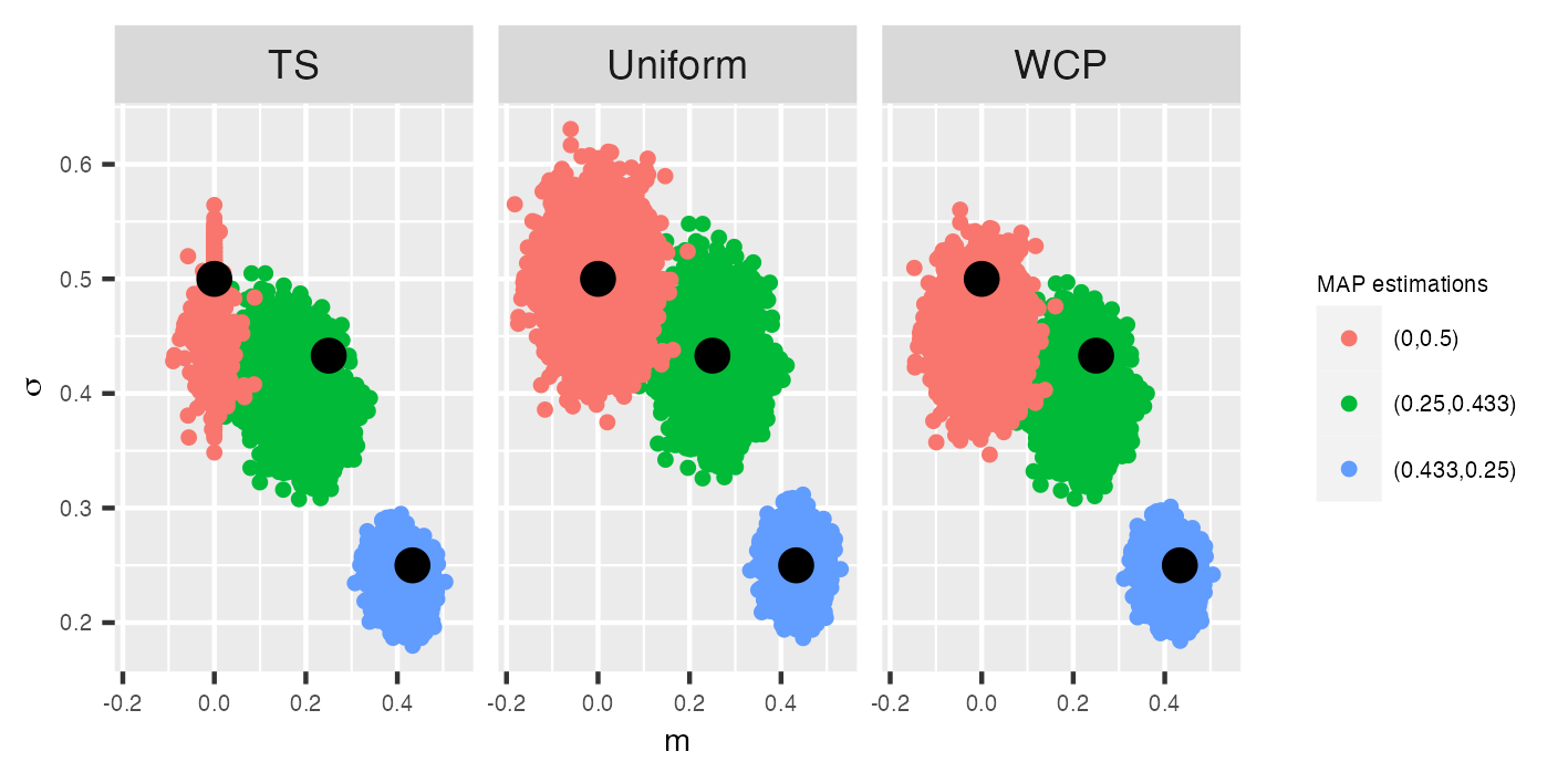
Figure 7: MAP estimations of the pairs $(m=0,\sigma=0.5)$, $(m=0.25,\sigma=0.433)$ and ${(m=0.433,\sigma=0.25)}$ under two-step approach prior (TS), uniform prior and $\text{WCP}_{2}$ prior. The black dots represent the true values of the parameter pair and the colored points clouds are the corresponding MAP estimates.

It should be noted that it is hard to compare the WCP prior and its two-step approximation fairly because the WCP prior has one user-specified hyperparameter whereas the two-step prior has two. In Figure 7, the two hyperparameters for the two-step prior was chosen to be the same as the one from the WCP prior. However, one could choose the two user-specified hyperparameters separately, as discussed in Fuglstad et al. (2019, Section 2.2). See Appendix A for further details.

4.4 A general recipe for deriving multivariate WCP priors

To conclude the discussion on multivariate WCP priors, we provide a recipe for computing multivariate WCP priors under Assumption 2. The recipe is inspired by the results in Jensen et al. (2001, Section 4.2). In the recipe, all notations have the same meaning as in Assumption 2 and Definition 3.

Recipe 2.

Suppose that we have a model with $n$ parameters $\boldsymbol{\theta}=(\theta_{1},\ldots,\theta_{n})$, and that the level set $S_{w}$ admits a parameterization $\alpha(\boldsymbol{\theta}_{-n};w)=(\alpha_{1}(\boldsymbol{\theta}_{-n};w),...,\alpha_{n}(\boldsymbol{\theta}_{-n};w))$ for each $w>0$, where $\theta_{-n}=[\theta_{1},...,\theta_{n-1}]$.

1. Compute $|d\alpha(\boldsymbol{\theta}_{-n};w)|=\sqrt{\det[J_{\alpha}(\boldsymbol{\theta}_{-n})^{\top}J_{\alpha}(\boldsymbol{\theta}_{-n})]}$, where $J_{\alpha}(\boldsymbol{\theta}_{-n})$ denotes the Jacobian of $\alpha$ evaluated at $\boldsymbol{\theta}_{-n}$.

2. Compute $\{u_{i,w}\}_{i=1}^{n-1}$ as

   $$u_{1,w} =u_{1}(\theta_{1};w)=\frac{\int_{\inf\Theta_{1}}^{\theta_{1}}\int_{\boldsymbol{\theta}_{2:n-1}}|d\alpha(x,\theta_{2:n-1};w)|\text{d}x\text{d}\theta_{2}...\text{d}\theta_{n-1}}{\int_{\boldsymbol{\Theta}}|d\alpha(x,\theta_{2:n-1};w)|\text{d}x\text{d}\theta_{2}...\text{d}\theta_{n-1}},$$

   $$u_{i,w} =u_{i}(\theta_{i};\theta_{1:i-1},w)=\frac{\int_{\inf\Theta_{i}}^{\theta_{i}}\int_{\boldsymbol{\theta}_{i+1:n-1}}|d\alpha(\theta_{1:i-1},x,\theta_{i+1:n-1};w)|\text{d}x\text{d}\theta_{i+1}...\text{d}\theta_{n-1}}{\int_{\boldsymbol{\theta}_{i:n-1}}|d\alpha(\theta_{1:i-1},x,\theta_{i+1},...,\theta_{n-1};w)|\text{d}x\text{d}\theta_{i+1}...\text{d}\theta_{n-1}}$$

   for $i=2,...,n-1$. Here $\theta_{i:j}$ denotes a vector $[\theta_{i},\theta_{i+1},...,\theta_{j}]$ and $\int_{\boldsymbol{\theta_{i:j}}}$ denotes an integral over the Cartesian product of $\boldsymbol{\theta}_{i},\boldsymbol{\theta}_{i+1},...,\boldsymbol{\theta}_{j}$.

3. Assign uniform distributions to $\{u_{i,w}\}_{i=1}^{n-1}$ and (truncated) exponential distribution to $w$ and finally do a change of variable to obtain the multivariate WCP prior density of $\boldsymbol{\theta}$.

Appendix B provides a concrete example of using this recipe to derive a three-dimensional WCP prior for the covariance parameters of a centered bivariate Gaussian distribution.

5 Numerical approximation of multivariate WCP prior

The goal is now to obtain approximate WCP priors for cases when they are not analytically tractable. To simplify the exposition, we limit the scope to univariate and bivariate priors.

5.1 Univariate priors

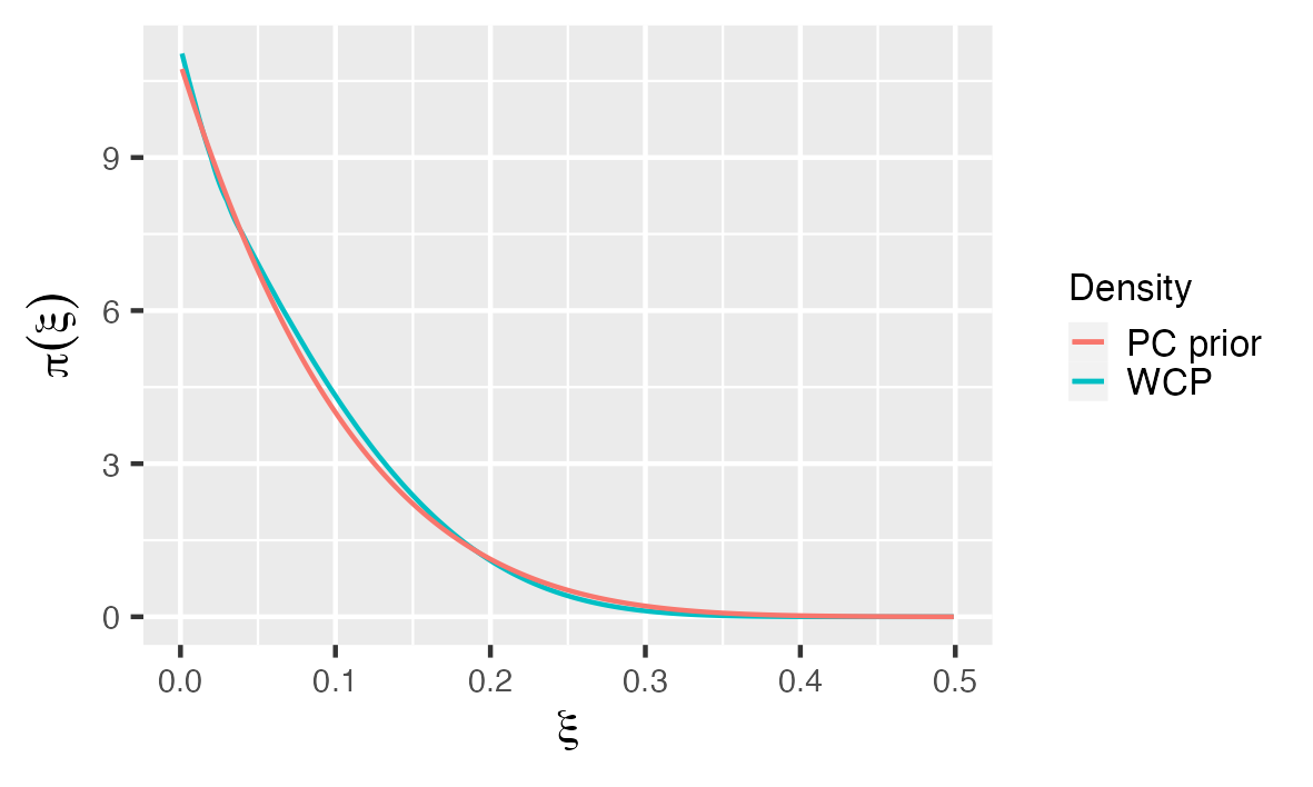
Figure 8: The $\text{WCP}_{2}$ prior and PC prior of reciprocal of the degree of freedom of t-distribution. All the prior densities satisfy that $P(\xi>0.2)=0.1$.

As a motivating example, suppose we want to obtain the WCP₂ prior for the degrees of freedom $\nu$ of a Student’s t-distribution with density

$$\pi(x;\nu)=\frac{\Gamma(\frac{\nu+1}{2})}{\sqrt{\nu\pi}\Gamma(\nu/2)}(1+x^{2}/\nu)^{-\frac{\nu+1}{2}},$$

where $\Gamma(\cdot)$ is the Gamma function. When $\nu\rightarrow\infty$, the t-distribution becomes the standard Gaussian distribution, which we consider as base model. To this end, let $\xi=1/\nu$, so that the base model corresponds to $\xi=0$. In this case we do not have closed-form expression for the Wasserstein distance between the flexible and base model, even if we apply Remark 1. Thus, a numerical approximation is necessary. The following recipe provides a strategy for obtaining such an approximation. Here we assume $\Theta_{-}=\emptyset$ and $\Theta_{+}=(\theta_{0},\infty)$, see Definition 2, but an adaptation of the recipe for the remaining cases is straightforward.

Recipe 3.

Let $\theta$ denote the parameter for a flexible model, $\theta_{0}$ denote the parameter for the base model and $\Theta=\Theta_{+}$ be the set of possible values of $\theta$. Let $\hat{W}_{p}(\theta)$ denote the (exact or approximated) Wasserstein-$p$ distance, computed by using Remark 4, between a flexible model with parameter $\theta$ and the base model. The following hyperparameters must be determined by the user: $\eta>0$, which controls the tail mass of the prior; $\delta>0$, which is a cutoff parameter; and $\epsilon>0$, which is the mesh width. Let $w^{*}=-\log(\delta)/\eta$ and compute the approximation as follows:

1. Following Remark 4, compute $\hat{W}_{p}(\theta)$, find $N^{\ast}:=\min\{N\in\mathbb{N}:\hat{W}_{p}(N)\geq w^{*}\}$, and perform a binary search on $[N^{*}-1,N^{*}]$ to find $z^{*}\in[N^{*}-1,N^{*}]$ satisfying $\hat{W}_{p}(z^{*})\geq w^{*}$ and $\hat{W}_{p}(z^{*}-\epsilon)<w^{*}$.

2. Create a regular mesh of $[\theta_{0},z^{*}]$ with $\lceil z^{*}/\epsilon\rceil$ terms, and denote it by $P_{z^{*},\epsilon}$.

3. Compute the numerical derivative $\hat{D}_{\epsilon}\hat{W}_{p}(\theta)=\frac{\hat{W}_{p}(\theta+\varepsilon)-\hat{W}_{p}(\theta)}{\varepsilon}$ for $\theta\in P_{z^{*},\epsilon}$.

4. Compute $\hat{c}:=\sup_{\theta>\theta_{0}}W_{p}(\theta)$ to order $O(\epsilon^{2})$. Define $\hat{c}=\infty$ if there is $N>0$ such that $W_{p}(N)>-\log(\epsilon^{2}/(1+\epsilon^{2}))/\eta$.

5. Approximate the $WCP_{p}$ density by $\hat{\pi}(\theta)=|\hat{D}_{\epsilon}\hat{W}_{p}(\theta)|\eta\exp(-\eta\hat{W}_{p}(\theta))/(1-\exp(\eta\hat{c}))$, for $\theta\in P_{z^{*},\epsilon}$.

6. Let $\tilde{\pi}_{\epsilon,\delta}(\theta)$ be the final approximation, obtained by linear interpolation of $\hat{\pi}(\theta)$ on $[\theta_{0},z^{*}]$, and extending as zero on $[\theta_{0},z^{*}]^{c}$.

The reason for the choice of $w^{*}$ is that if $W\sim Exp(\eta)$, then $P(W>w^{*})=\delta$.

Remark 4.

If one has probability measures on $\mathbb{R}$, one can use Remark 1 to either obtain an analytical expression or a numerical approximation for $W_{p}(\theta)$. If using a numerical approximation, obtain a numerical approximation such that the error is of order $O(\epsilon^{2})$, for example using trapezoidal rule of numerical integration. On the other hand, for more general measures, if the base model is a Dirac measure, one can use Proposition 1 instead. Finally, in practice, due to the exponential decay, $N^{*}$ is small.

Example 8.

An approximation of the WCP₂ prior density for $\nu$ in the t-distribution, obtained using the recipe and Remark 4, is shown in Figure 8. The figure also shows an approximation of the PC prior density from Simpson et al. (2017, Supplementary material), which also required numerical approximation to compute. Simpson et al. (2017) compared the PC prior, an exponential prior and uniform prior of $\nu$ for $\nu>2$, that is $\xi\in[0,1/2)$. They showed that neither the exponential prior nor the uniform prior can not have their mode at the base model while the PC prior has this property by design. The WCP₂ prior also has this property.

We have the following proposition regarding the approximated density obtained by applying Recipe 3, which provides a rigorous theoretical justification for such recipe.

Proposition 7.

Let Assumption 1 hold, and consider the same notations and assumptions from Recipe 3. Also assume that $W_{p}(\cdot)$ is an increasing function of class $C^{2}$. Let $\tilde{\pi}_{\epsilon,\delta}(\cdot)$ be the approximate density obtained by Recipe 3 and $\pi(\cdot)$ be the true WCP prior density. Then, there exists a constant $C>0$ that does not depend on $\epsilon$, but might depend on $\delta$, such that for sufficiently small $\epsilon>0$

$$\int_{\mathbb{R}}|\tilde{\pi}_{\epsilon,\delta}(\theta)-\pi(\theta)|d\theta\leq C\epsilon+\delta.$$

In particular, $\lim_{\delta\to 0}\lim_{\epsilon\to 0}\int_{\mathbb{R}}|\tilde{\pi}_{\epsilon,\delta}(\theta)-\pi(\theta)|d\theta=0.$

Remark 5.

If $\Theta$ is bounded, one can start with step 3 of Recipe 3, where a regular mesh of $\Theta$ is created instead. In this case we have $\delta=0$.

5.2 Bivariate priors

Recall Definition 3 of the multivariate WCP priors and Recipe 1. For a model with two parameters $\boldsymbol{\theta}=[\theta_{1},\theta_{2}]$ with domain $\boldsymbol{\Theta}\subset\mathbb{R}^{2}$, there are a number of components required to obtain the prior: $W_{p}(\boldsymbol{\theta})$, the Wasserstein distance evaluated at $\boldsymbol{\theta}$; $u_{1}(\theta_{1};W_{p}(\boldsymbol{\theta}))$, the partial arc length evaluated at $\boldsymbol{\theta}$ of the level curve $S_{W_{p}(\boldsymbol{\theta})}$; $l(S_{W_{p}(\boldsymbol{\theta})})$, the total arc length of $S_{W_{p}(\boldsymbol{\theta})}$ and finally, the determinant of Jacobian $J_{W_{p},u_{1}}(\boldsymbol{\theta})$ which requires the first order derivative of $W_{p}(\boldsymbol{\theta})$ and $u_{1}(\theta_{1};W_{p}(\boldsymbol{\theta}))$ concerning the two parameters evaluated at $\boldsymbol{\theta}$.

One or several of these components may be difficult to compute analytically, and we now provide a numerical method for approximating the prior.

The method is more elaborate than its counterpart for univariate priors, that is, Recipe 3. Therefore, we provide the recipe here, but most of the technical details are provided as algorithms in Appendix D.

Recipe 4.

The user needs to specify some controlling hyperparameters, $\eta>0$ that controls the tail mass, $\tau>0$ and $0<\delta<1$ which are cutoff parameters and $\tilde{\epsilon}>0$, which controls the order for approximating the Wasserstein distances and $\epsilon>0$, which is the mesh width for approximating the partial arc lengths. Further, let $\hat{W}_{p}(\boldsymbol{\theta})$ denote the (exact or approximated) Wasserstein-$p$ distance, computed by using Remark 4, between a flexible model with parameter $\boldsymbol{\theta}$ and the base model (which has parameter $\boldsymbol{\theta}_{0}$).

1. Use Remark 4 to compute the necessary Wasserstein distances with order $O(\tilde{\epsilon}^{2})$.

2. Let $w^{*}=-\log(\delta/2)/\eta$ and $w_{*}=\hat{W}_{p}(\boldsymbol{\theta}_{0}+\tau\boldsymbol{v})-\log(1-(\delta+\tau)/2)/\eta$, where $\boldsymbol{v}\in\mathbb{R}^{2}$, $\|\boldsymbol{v}\|_{\mathbb{R}^{2}}=1$, is any direction such that $\boldsymbol{\theta}_{0}+\tau\boldsymbol{v}$ belongs to the interior of $\boldsymbol{\Theta}$.

3. Use Algorithm 3 in Appendix D to find a compact region $\Pi_{\tilde{\epsilon},\delta,\tau}\subset\boldsymbol{\Theta}$ such that there exists some constant $C>0$, that does not depend on $\tilde{\epsilon},\delta$ nor on $\tau$, so that if $\boldsymbol{\theta}\not\in\Pi_{\tilde{\epsilon},\delta,\tau}$, then $W_{p}(\boldsymbol{\theta})>w^{*}-C\tilde{\epsilon}^{2}$ or $W_{p}(\boldsymbol{\theta})<w_{*}+C\tilde{\epsilon}^{2}$.

4. Let $\Delta_{\tilde{\epsilon},\delta,\tau}=\Pi_{\tilde{\epsilon},\delta,\tau}\cap\{\boldsymbol{\theta}\in\boldsymbol{\Theta}:d(\boldsymbol{\theta},\partial\boldsymbol{\Theta})\geq\tau\},$ where $d(x,A):=\inf\{\|x-y\|_{\mathbb{R}^{2}}:y\in A\}$, $\|\cdot\|_{\mathbb{R}^{2}}$ is the Euclidean norm on $\mathbb{R}^{2}$ and $\partial\boldsymbol{\Theta}$ is the boundary of $\boldsymbol{\Theta}$.

5. Create a quasi-uniform triangular mesh in $\Delta_{\tilde{\epsilon},\delta,\tau}$ with mesh width $\tilde{\epsilon}$ and denote it by $\Delta_{\tilde{\epsilon},\delta,\tau}^{\tilde{\epsilon}}$. Let $G_{\tilde{\epsilon}}$ denote the set of its mesh nodes.

6. Compute $\hat{W}_{p}(\boldsymbol{\theta})$ for every $\boldsymbol{\theta}\in G_{\tilde{\epsilon}}$. Further, use the same numerical approximation to obtain values of $\hat{W}_{p}(\boldsymbol{\theta})$ at any other needed additional locations in $\Delta_{\tilde{\epsilon},\delta,\tau}$.

7. Use this approximation together with Algorithm 4 in Appendix D to compute $u_{1}(\cdot;\cdot)$, $l(\cdot)$ and the Jacobian term, based on a discretization with mesh width $\epsilon>0$.

8. Use these approximations in (6) to obtain an approximation of the WCP_p density on $G_{\epsilon}$.

9. Let $\tilde{\pi}_{\epsilon,\tilde{\epsilon},\delta,\tau}$ be the density obtained by linear interpolating the previous results in $\Delta_{\tilde{\epsilon},\delta,\tau}$, and extending as zero on $\mathbb{R}^{2}\setminus\Delta_{\tilde{\epsilon},\delta,\tau}$.

We have the following result regarding the approximated density obtained by the numerical recipe for 2d WCP priors, whose proof can be found in Appendix E. For the statement, we need the following definitions. We say that $W_{p}(\cdot)$ is strictly increasing in all directions around $\boldsymbol{\theta}_{0}$ if for every $\boldsymbol{v}\in\mathbb{R}^{2}$ with $\|v\|_{\mathbb{R}^{2}}=1$ such that for some $t^{*}>0$, $\boldsymbol{\theta}_{0}+t^{*}\boldsymbol{v}$ belongs to $\boldsymbol{\Theta}$, we have that whenever $0<t_{1}<t_{2}$ are such that $\boldsymbol{\theta}_{0}+t_{1}\boldsymbol{v}\in\boldsymbol{\Theta}$ and $\boldsymbol{\theta}_{0}+t_{2}\boldsymbol{v}\in\boldsymbol{\Theta}$, we also have $W_{p}(\boldsymbol{\theta}_{0}+t_{1}\boldsymbol{v})<W_{p}(\boldsymbol{\theta}_{0}+t_{2}\boldsymbol{v})$. For a given level curve $S_{w}$ and $\tau>0$, let $S_{w}^{\tau}:=S_{w}\cap\{\boldsymbol{\theta}\in\boldsymbol{\Theta}:d(\boldsymbol{\theta},\partial\boldsymbol{\Theta})\geq\tau\}$.

Proposition 8.

Let Assumption 2 hold and also let the assumptions in Recipe 2 hold. Additionally, assume that $\boldsymbol{\theta}\mapsto W_{p}(\boldsymbol{\theta})$ is of class $C^{2}$ on $\boldsymbol{\Theta}$. If using a numerical approximation of $W_{p}(\cdot)$, we assume that the error of the approximation is of order $O(\tilde{\epsilon}^{2})$. Further, assume that for every $\tau>0$, the function $w\mapsto l(S_{w}^{\tau})$ is strictly increasing and that for every $w>0$, the level curve $S_{w}$ is a graph of a function and the level curve starts and ends at the boundary of $\boldsymbol{\Theta}$ whose intersection with the boundary consists of at most two points. Furthermore, assume that either the level sets of $W_{p}(\cdot)$ are straight lines passing through $\boldsymbol{\theta}_{0}$ or that $W_{p}(\cdot)$ is strictly increasing in all directions around $\boldsymbol{\theta}_{0}$. Then, there exists a constant $C>0$ that does not depend on $\epsilon$, but might depend on $\delta$ and $\tau$, such that for sufficiently small $0<\tilde{\epsilon}<\epsilon$,

$$\int_{\mathbb{R}^{2}}|\tilde{\pi}_{\epsilon,\tilde{\epsilon},\delta,\tau}(\boldsymbol{\theta})-\pi(\boldsymbol{\theta})|d\boldsymbol{\theta}\leq C\left(\epsilon+\tilde{\epsilon}+\frac{\tilde{\epsilon}}{\epsilon}\right)+\frac{3}{2}\delta+m_{\tau},$$

where $\tilde{\pi}_{\epsilon,\tilde{\epsilon},\delta,\tau}(\cdot)$ is the approximate density obtained by Recipe 4, $\pi(\cdot)$ is the true WCP prior density and $m_{\tau}$ depends on $\delta$ and satisfies, for fixed $\delta>0$, $\lim_{\tau\to 0}m_{\tau}=0$. In particular, for any choice of $\tilde{\epsilon}<\epsilon$ such that $\tilde{\epsilon}=o(\epsilon)$, we have

$$\lim_{\delta\to 0}\lim_{\tau\to 0}\lim_{\epsilon\to 0}\int_{\mathbb{R}^{2}}|\tilde{\pi}_{\epsilon,\tilde{\epsilon},\delta,\tau}(\boldsymbol{\theta})-\pi(\boldsymbol{\theta})|d\boldsymbol{\theta}=0.$$

Remark 6.

By following Proposition 6 and Corollary 1, we obtain that Proposition 8 also holds for any region satisfying the assumptions of Corollary 1. In particular, it holds for the conic regions in Corollary 1.

Remark 7.

There are a number of important remarks to be made about the proof of Proposition 8. This proof is difficult and long as it deals with several uncommon problems. The first is that it involves three parameters that control different aspects of the approximation; $\epsilon>0$ that controls the mesh width, $\tau>0$ that controls the distance to the boundary and $\delta>0$ that controls the cutoff. The fact that we have three parameters that control the approximation and that we want to send them all to zero (in a specific order) means that we need to be very careful with the dependency of the parameters when obtaining the bounds. Another difficulty comes from the fact that we want to approximate level curves, but they are given implicitly. This requires an indirect approximation which requires some quantities to being finite or bounded away from zero. This is where the parameter $\tau$ appears, since these quantities are finite and bounded away from zero in the interior of the domain but might not be so at the boundary.

A problem that constantly appears in the proof is that we compute the partial arc lengths on level curves with distance $\tau$ from the boundary. This means that we do not approximate two very small pieces of the level curves, which consists of points of the level curves that are at distance less than $\tau$ from the boundary. Therefore, we need to show that these parts are negligible as $\tau$ tends to zero, which involves making sure that we can bound it by a constant that does not depend on $\tau$. The final difficulty comes from the fact that the level curves with total arc length close to zero are problematic as they make it impossible to obtain some bounds. Thus, we need to remove level curves with very small total arc lengths, having a lower bound on the smallest possible arc length that does not depend on $\tau$ and also make sure that the removed part is negligible.

Remark 8.

In practice, when implementing the numerical recipe, the choice $\tau=\epsilon/1000$ typically provides good results. Furthermore, even though we needed $\tilde{\epsilon}=o(\epsilon)$ to prove the theoretical convergence, we found that in practice the choice $\tilde{\epsilon}=\epsilon$ provides very good numerical approximations. Thus, we recommend, as a general rule of thumb, $\tau=\epsilon/1000$ and $\tilde{\epsilon}=\epsilon$.

Example 9.

To illustrate this numerical recipe, we use it to approximate two bivariate WCP₂ prior for the mean and standard deviation parameter of Gaussian distribution (recall Example 4). We denote the mean parameter as $\theta_{1}$ and the standard deviation parameter as $\theta_{2}$. We fix $\eta=1$ for the prior and set the cutoff parameter $\delta=0.01$ in the recipe and consider mesh widths $\epsilon\in\{0.5,0.4,0.3,0.2,0.1\}$ with $\tilde{\epsilon}=\epsilon$ and $\tau=\epsilon/1000$. In the recipe, we approximate $W_{2}(\boldsymbol{\theta})$ using Remark 4 and numerical integration. To see how well this numerical approximation works, we assess the total variation (TV) distance between the analytical WCP₂ prior (4) and the numerical approximation. The TV distance between two probability measures $P_{1}$ and $P_{2}$ on a common $(\Omega,\mathcal{F})$ is defined by $TV(P_{1},P_{2})=\sup_{A\in\mathcal{F}}|P_{1}(A)-P_{2}(A)|$ and provides an upper bound of the difference between two probability measures’ evaluations of the measurable sets from $\mathcal{F}$. Let $p_{1},p_{2}$ be the probability densities of $P_{1},P_{2}$ with respect to the Lebesgue measure $\lambda$. Then, ${TV(P_{1},P_{2})=\frac{1}{2}\int|p_{1}-p_{2}|\text{d}\lambda}$ (Levin and Peres, 2017, Proposition 4.2). We approximate the integral numerically based on the mesh for the approximate density. The left panel of Figure 9 shows that the TV distance between $P_{1}$ and $P_{2}$ decreases with the mesh width as expected.

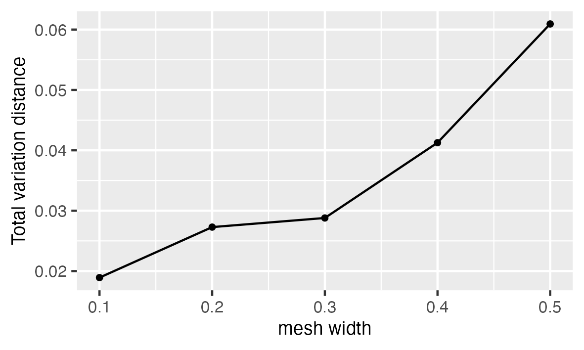
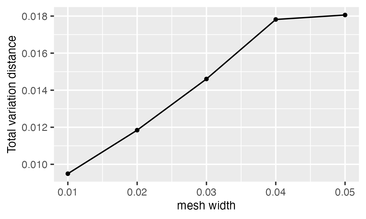
Figure 9: TV distances between the true and approximate WCP priors as functions of the mesh with. The left panel shows the case of the WCP₂ prior for the Gaussian distribution in Example 9 and the right panel shows the WCP₁ prior for the Pareto distribution in Example 10.

Example 10.

To further illustrate the numerical recipe, we use it to approximate the bivariate WCP₁ prior for $\boldsymbol{\theta}=(\sigma,\xi)$ of the generalized Pareto distribution (recall Example 5). We fix $\eta=20$ for the prior, and use $\tau=0.001$ and $\delta=0.01$ in the recipe. We consider mesh widths ${\epsilon\in\{0.05,0.04,0.03,0.02,0.01\}}$ with $\tilde{\epsilon}=\epsilon$. Similar with Example 9, we assess the TV distance between the analytical WCP₁ prior (7) and the numerical approximation. The right panel of Figure 9 shows that the distance decreases with the mesh width as expected.

6 Discussion

We have introduced the WCP priors for models with a single parameter and their extension to models with multiple parameters. By replacing the KLD with the Wasserstein distance, we can measure the departure of flexible models away from the base model by computing the true value of the distance, thus overcoming several drawbacks of the original PC priors. As a result, we obtain a prior that truly follows its principles. We also showed that the WCP priors are mathematically tractable and practical to use. On one hand, Remark 1 and Proposition 1 indicate that one can actually compute the Wasserstein distance analytically or by numerical integration in many common cases including cases with multiple parameters and/or when the base model does not induce a Dirac measure. Therefore, typically, the evaluation of the Wasserstein distance should not be an obstacle. We further provided recipes for computing multivariate WCP priors analytically. On the other hand, we also provided numerical recipes for approximating the WCP priors when it is not possible or feasible to obtain it analytically.

We provided several examples of WCP priors for models where PC priors previously have been derived. One important example which we have not considered is WCP priors for random fields such as Whittle–Matérn fields on bounded subsets of $\mathbb{R}^{d}$. This is currently being investigated. An important question for future work related to this is how to adjust the WCP prior framework to multiple base models, which is relevant in cases where one might want to have the base models supported on integer values when obtaining a prior for a real valued parameter.

Appendix A Further numerical studies on two-step WCP priors

In this section, we provide additional results for the simulation study in Section 4.3. We first compare the two-dimensional WCP prior for the generalized Pareto distribution studied in Example 5 and its two-step approach $\text{WCP}_{2}$ prior in a simulation study. We choose the true pair of parameters $(\sigma,\xi)$ from the same level curve of the Wasserstein distance and compute their MAP estimations with 100 independent and identically distributed samples for 5000 rounds. Figure 10 shows the MAP estimations result for generalized Pareto distribution. Comparing to the uniform prior, the MAP estimations under WCP prior and its two-step prior are attracted toward different locations. The WCP prior attracts the MAP estimations towards the Y-axis, where the true base model is, while the two-steps prior attracts them towards the point $\sigma=0,\xi=0$. This result also fits well with the density plots from Figure 4 and Figure 6.

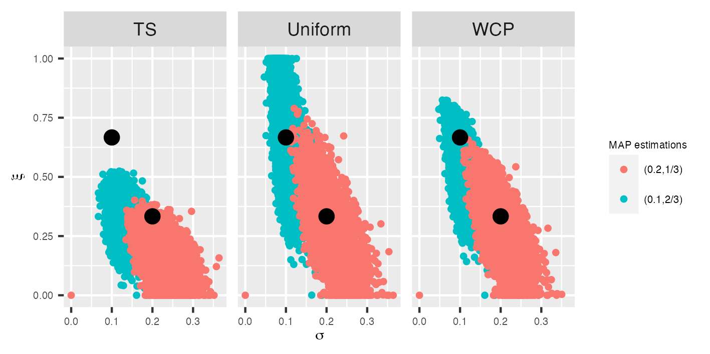
Figure 10: MAP estimations of the pairs $\sigma=0.2,\xi=1/3$ and ${\sigma=0.1},{\xi=2/3}$ under two-steps approach prior (TS), uniform prior and $\text{WCP}_{1}$ prior. The black dots represent the true values of the parameter pairs and the colored points clouds are the corresponding MAP estimations.

As mentioned in Section 4.3, the two-step WCP prior is different from the WCP prior in nature and has more user-specified hyperparameters. This gives the two-step approach more freedom to penalize each parameters in different ways. To illustrate this, we perform similar simulation studies for Gaussian distribution and generalized Pareto distribution under two-step WCP priors with different choice of user-specified hyperparameters from different steps. Figure 11 shows the MAP estimations of three pairs of parameters of Gaussian distribution under three different two-step WCP priors. The first one choose $\eta_{1}=\eta_{2}=46.0517$, the second one choose $\eta_{1}=4.60517,\eta_{2}=46.0517$ and the third one choose $\eta_{1}=46.0517,\eta_{2}=4.60517$. The second prior penalizes more on $\sigma$ than $\mu$ while the third prior penalizes more on $\mu$ than $\sigma$. This can be easily seen by comparing the shape of the red points clouds from the figure. The red point cloud from the second prior has the widest range in $\mu$ while the one from the third prior has the widest range in $\sigma$.

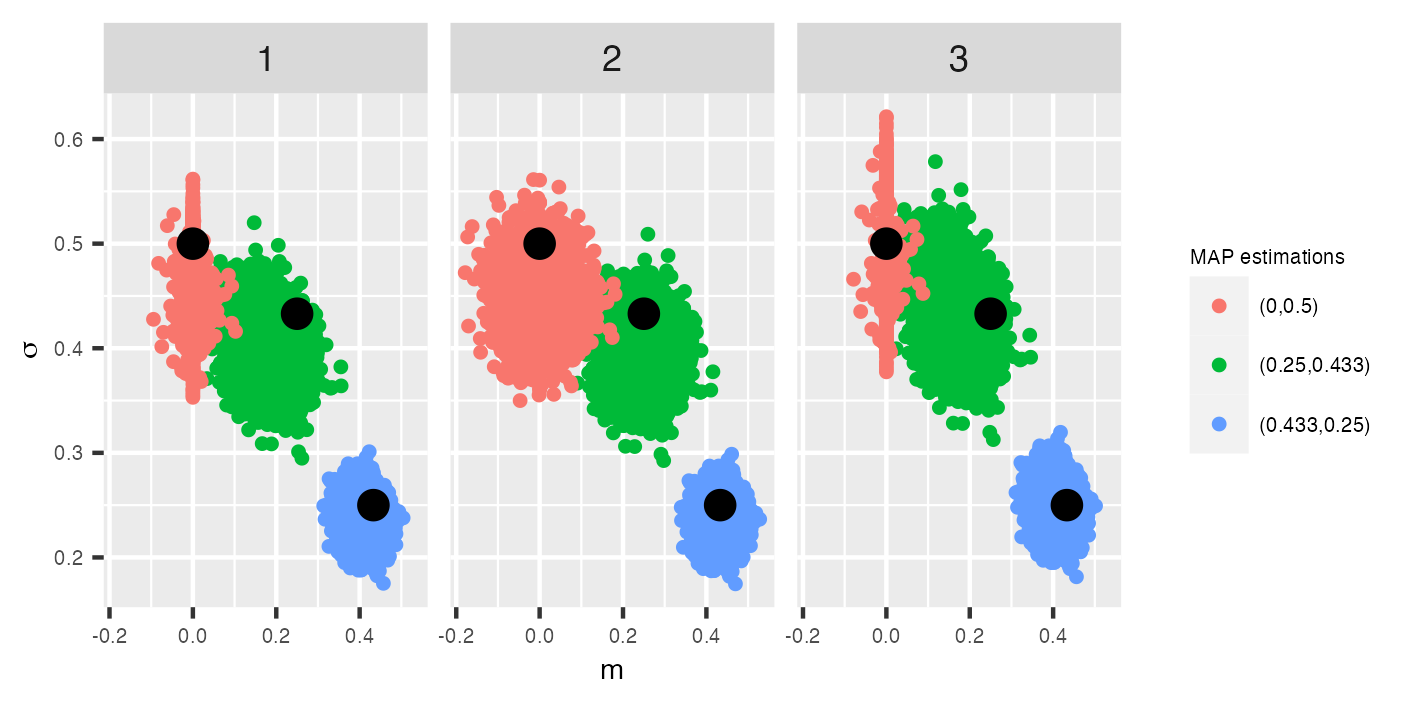
Figure 11: MAP estimations of the pairs $m=0,\sigma=0.5$, $m=0.25,\sigma=0.433$, $m=0.433$, ${\sigma=0.25}$ under different two-steps WCP priors. The black dots represent the true values of the parameter pairs and the colored points clouds are the corresponding MAP estimations.

A similar result from the generalized Pareto distribution case is shown in Figure 12. The first prior choose $\eta_{1}=\eta_{2}=10$, the second one choose $\eta_{1}=10,\eta_{2}=80$ and the third one choose $\eta_{1}=80,\eta_{2}=10$. The second prior penalizes more on $\xi$ than $\sigma$ while the third prior penalizes more on $\sigma$ than on $\xi$.

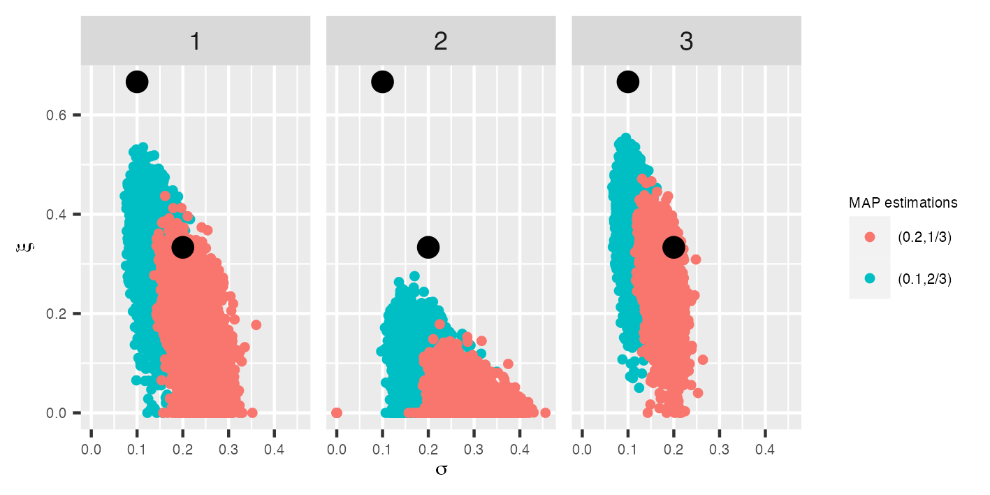
Figure 12: MAP estimations of the pairs $\sigma=0.2,\xi=1/3$ and ${\sigma=0.1},{\xi=2/3}$ under different two-step WCP priors. The black dots represent the true values of the parameter pairs and the colored points clouds are the corresponding MAP estimations.

Appendix B An example of three-dimensional WCP prior

In this section, we consider a three-dimensional WCP₂ prior for three parameters of a zero mean bivariate Gaussian distribution. For a zero mean two-dimensional Gaussian random vector $Z=[z_{1},z_{2}]^{\top}$, we can use three parameters to characterize its distribution: $\sigma_{1}\sigma_{2},\rho$. $\sigma_{i}\geq 0$ is the standard deviation of $z_{i}$ for $i=1,2$ and $\rho\in[-1,1]$ denotes the correlation coefficients between $z_{1}$ and $z_{2}$. The base model parameters that induce a Dirac measure concentrate at $Z=[0,0]^{\top}$ are $\sigma_{1}=\sigma_{2}=\rho=0$. The Wasserstein-2 distance between the base model and a flexible model is $W_{2}(\sigma_{1},\sigma_{2},\rho)=(\sigma_{1}^{2}+\sigma_{2}^{2})^{1/2}$. By fixing $W_{2}(\sigma_{1},\sigma_{2},\rho)$ to a positive value $w$, we obtain a level surface $S_{w}$ that can be parameterized as $\alpha(\rho,\sigma_{1})=(\sigma_{1},w^{2}-\sigma_{1}^{2},\rho),\sigma_{1}\in[0,w],\rho\in[-1,1]$. Then, by following Recipe 2:(2), we calculate

$$u_{1}(\rho;w) =\frac{\int_{-1}^{\rho}\int_{0}^{w}\sqrt{1+\frac{\sigma_{1}^{2}}{w^{2}-\sigma_{1}^{2}}}\text{d}\sigma_{1}\text{d}x}{\int_{-1}^{1}\int_{0}^{w}\sqrt{1+\frac{\sigma_{1}^{2}}{w^{2}-\sigma_{1}^{2}}}\text{d}\sigma_{1}\text{d}\rho}=\frac{\rho+1}{2},$$

$$\quad u_{2}(\sigma_{1};\rho,w) =\frac{\int_{0}^{\sigma_{1}}\sqrt{1+\frac{x^{2}}{w^{2}-x^{2}}}\text{d}x}{\int_{0}^{w}\sqrt{1+\frac{\sigma^{2}}{w^{2}-\sigma^{2}}}\text{d}\sigma}=\frac{2}{\pi}\tan^{-1}(\frac{\sigma_{1}}{\sqrt{w^{2}-\sigma_{1}^{2}}}).$$

By Recipe 2:(3),the joint $\text{WCP}_{2}$ prior of $w,u_{1}$ and $u_{2}$ is $\pi_{w,u1,u2}(w,u_{1},u_{2})=\eta\exp(-\eta w)$, and by a change of variables we obtain the $\text{WCP}_{2}$ of $\sigma_{1},\sigma_{2}$ and $\rho$ as:

$$\pi_{\sigma_{1},\sigma_{2},\rho}(\sigma_{1},\sigma_{2},\rho)=\frac{1}{(\sigma_{1}^{2}+\sigma_{2}^{2})^{1/2}\pi}\eta\exp(-\eta(\sigma_{1}^{2}+\sigma_{2}^{2})^{1/2}).$$

Since this three dimensional density does not change with respect to value of $\rho$, Figure 13 shows a slice of it in log scale by fixing $\rho$ to a constant.

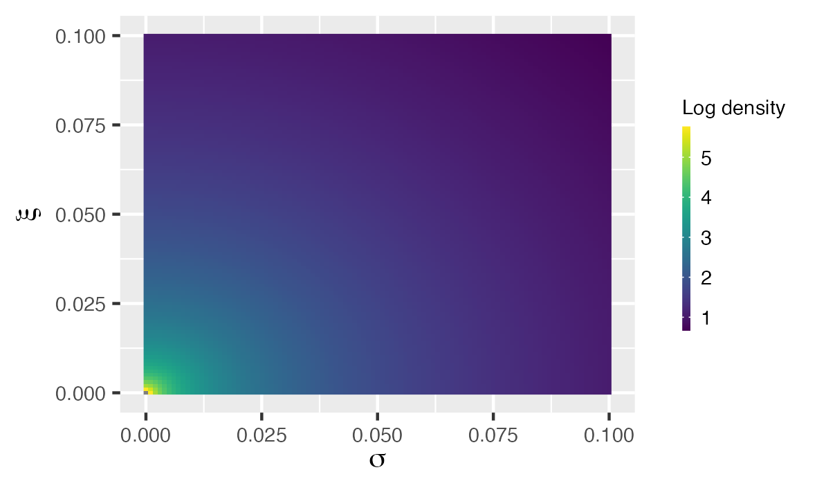
Figure 13: Log $\text{WCP}_{2}$ prior density of $\sigma_{1}$ and $\sigma_{2}$ with a fixed $\rho$ and $\eta=1$.

Appendix C Proof of Proposition 7

Fix $\delta>0$ and consider the quantities defined in Recipe 3. Let $\Theta_{\delta}$ denote $[\theta_{0},z^{*}]$, we start by bounding the difference on $\Theta_{\delta}^{c}:=\mathbb{R}\setminus\Theta_{\delta}$. Note that since, by assumption, $W_{p}(\cdot)$ is increasing, if $\theta>z^{*}$, then $W_{p}(\theta)>w^{*}$. We then have that

$$\int_{\Theta_{\delta}^{c}}\pi(\theta)d\theta\leq P(W>w^{*})=\delta,$$ (8)

where $W\sim Exp(\eta)$. Let us now bound the difference $|\tilde{\pi}_{\epsilon,\delta}(\theta)-\pi(\theta)|$, for $\theta\in\Theta_{\delta}$. By assumption, there exists some constant $C_{\delta}>0$ such that for any $\theta\in\Theta_{\delta}$,

$$|W_{p}(\theta)-\hat{W}_{p}(\theta)|\leq C_{\delta}\epsilon^{2}.$$ (9)

Further, we have, by the mean value theorem,

$$|\hat{D}_{\epsilon}\hat{W}_{p}(\theta)-W_{p}^{\prime}(\theta)| \leq\left|\frac{\hat{W}_{p}(\theta+\epsilon)-\hat{W}_{p}(\theta)}{\epsilon}-W_{p}^{\prime}(\theta)\right|=\left|\frac{W_{p}(\theta+\epsilon)-W_{p}(\theta)+H_{\delta}(\theta)}{\epsilon}-W_{p}^{\prime}(\theta)\right|$$

$$=\left|\frac{H_{\delta}(\theta)}{\epsilon}+W_{p}^{\prime}(c_{\theta})-W_{p}^{\prime}(\theta)\right|\leq 2C_{\delta}\epsilon+|W_{p}^{\prime\prime}(\tilde{c}_{\theta})||c_{\theta}-\theta|$$

$$\leq(2C_{\delta}+K_{\delta})\epsilon,$$ (10)

where $c_{\theta}\in(\theta_{0},\theta_{0}+\epsilon)$, $\tilde{c}_{\theta}\in(\theta,c_{\theta})$, $K_{\delta}:=\sup_{\theta\in\Theta_{\delta}}|W_{p}^{\prime\prime}(\theta)|<\infty$ and we have, by (9), ${|H_{\delta}(\theta)|\leq 2C_{\delta}\epsilon^{2}}$.

By the mean value theorem again, we have that for $x,y\in\mathbb{R}$, $x<y$, there exists $c\in(x,y)$ such that $|\exp(x)-\exp(y)|\leq\exp(c)|x-y|,$. Therefore,

$$|\exp\{-\eta\hat{W}_{p}(\theta)\}-\exp\{-\eta W_{p}(\theta)\}| \leq\exp\{-C\}|-\eta\hat{W}_{p}(\theta)+\eta W_{p}(\theta)|$$

$$\leq\eta|\hat{W}_{p}(\theta)-W_{p}(\theta)|\leq\tilde{C}_{\delta}\eta\epsilon^{2},$$ (11)

where $\tilde{C}_{\delta}>0$ is some constant and we used (9). If $\hat{c}=\infty$, then

$$\left|1-\frac{1}{1-\exp(-\eta\hat{c})}\right|<\epsilon^{2}.$$

Otherwise, we have $|\hat{c}-c|=O(\epsilon^{2})$, which gives us, for sufficiently small $\epsilon$,

$$\left|\frac{1}{1-\exp(-\eta\hat{c})}-\frac{1}{1-\exp(-\eta c)}\right|\leq C_{0}|c-\hat{c}|\leq\tilde{C}_{0}\epsilon^{2},$$

where $C_{0}=1/((1-\exp(-\eta W_{p}(\theta_{0}+1)))(1-\exp(-\eta W_{p}(\theta_{0}+1/2))))$, and $\hat{C}_{0}$ does not depend on $\epsilon$.

By (11) and the above inequalities, we have that there exists some constant $C_{\delta}>0$, depending only on $\delta$ such that for sufficiently small $\epsilon$,

$$\left|\frac{\exp\{-\eta\hat{W}_{p}(\theta)\}}{1-\exp\{-\eta\hat{c}\}}-\frac{\exp\{-\eta{W}_{p}(\theta)\}}{1-\exp\{-\eta c\}}\right|\leq C_{\delta}\eta\epsilon^{2}.$$ (12)

Therefore, by (10) and (12), we have for $\theta\in P_{z^{*},\epsilon}$ and $\epsilon<1$,

$$|\tilde{\pi}_{\epsilon,\delta}(\theta)-\pi(\theta)| \leq\left|\left(\hat{D}_{\epsilon}\hat{W}_{p}(\theta)-W_{p}^{\prime}(\theta)\right)\eta\frac{\exp\{-\eta\hat{W}_{p}(\theta)\}}{1-\exp\{-\eta\hat{c}\}}\right|$$

$$\quad+\left|W_{p}^{\prime}(\theta)\eta\left(\frac{\exp\{-\eta\hat{W}_{p}(\theta)\}}{1-\exp\{-\eta\hat{c}\}}-\frac{\exp\{-\eta W_{p}(\theta)\}}{1-\exp\{-\eta{c}\}}\right)\right|$$

$$\leq\eta\left|\hat{D}_{\epsilon}\hat{W}_{p}(\theta)-W_{p}^{\prime}(\theta)\right|+\sup_{\theta\Theta_{\delta}}|W_{p}^{\prime}(\theta)|C_{\delta}\eta\epsilon^{2}$$

$$\leq 2(C_{\delta}+K_{\delta})\epsilon+M_{\delta}\epsilon^{2}\leq\hat{M}_{\delta}\epsilon,$$ (13)

where $M_{\delta}:=\sup_{\theta\Theta_{\delta}}|W_{p}^{\prime}(\theta)|<\infty$, $\hat{M}_{\delta}<\infty$ only depends on $\delta$, and for the last inequality we used that $\epsilon<1$. Since $W_{p}(\cdot)\in C^{2}$, we have that $\pi(\cdot)\in C^{1}$. Thus, from (13), the mean value theorem, and linear interpolation of $\tilde{\pi}_{\epsilon,\delta}(\cdot)$, we have that for any $\theta\in[\theta_{0},z^{*}]$, $|\tilde{\pi}_{\epsilon,\delta}(\theta)-\pi(\theta)|\leq\tilde{M}_{\delta}\epsilon,$ where $\tilde{M}_{\delta}<\infty$ does not depend on $\epsilon$. Therefore,

$$\int_{\Theta_{\delta}}|\tilde{\pi}_{\epsilon,\delta}(\theta)-\pi(\theta)|\leq(z^{*}-\theta_{0})\tilde{M}_{\delta}\epsilon.$$ (14)

The result thus follows from combining (14) and (8).

Appendix D Auxiliary Algorithms for Recipe 4

We start with the algorithm to build the compact region $\Pi_{\epsilon,\delta,\tau}$ in Recipe 4. To simplify the exposition, we consider the unbounded conic region

$$\boldsymbol{\Theta}=\{(x,y)\in\mathbb{R}^{2}:(x,y)=(r\cos(\theta),r\sin(\theta)),r>0,\theta\in[0,\phi]\},\quad\phi\in(0,2\pi).$$

with the remaining cases being similar or simpler (for instance if $\boldsymbol{\Theta}$ is bounded). In Remark 9 we also describe how one can adjust Algorithm 3 for domains of the form $I\times[a,b]$, where the interval $I$ is unbounded.

The idea of the algorithm is to find an approximate level curve with level $w^{*}$ by first searching along the semi-lines with angles $\tilde{\epsilon}$ and $\phi-\tilde{\epsilon}$, and connect these points to create a line segment. This line segment is our first approximation of the level curve. We will now refine such approximation. In the next step we search on the semi-line in the mid angle $\phi/2$, starting from the intersection of this semi-line and the line segment obtained previously. We now connect the three points found to have the next approximation of the level curve. From this point on, the searches will be done sequentially for all the subsequent mid angles (for example, in the next step the angles considered will be $(\tilde{\epsilon}/2+\phi/4)$ and $(3\phi/4+\tilde{\epsilon/2})$), with the search starting at the intersection of these lines with the approximated level curve. This will determine an approximation of the level curve with $2^{N}$ segments, where $N$ is the number of subdivisions done. The algorithm stops when $\max\{\|\boldsymbol{\theta}_{i}-\boldsymbol{\theta}_{j}\|_{\mathbb{R}^{2}}:i,j=1,\ldots,2^{N}+1\}\leq\tilde{\epsilon}$, where $\boldsymbol{\theta}_{i}$, $i=1,\ldots,2^{N}+1$ are the points obtained by the algorithm after $N$ subdivisions. In the region construction, the following shift operator is used: $T_{t,\varphi}:\mathbb{R}^{2}\to\mathbb{R}^{2}$ given by $T_{t,\varphi}(x,y)=(x,y)+t(\cos(\varphi),\sin(\varphi))$.

Algorithm 1 LS$(\boldsymbol{\theta},s,w,\epsilon,W_{p}(\cdot))$ line search.

1:$\boldsymbol{\theta}$ (starting point), $s$ (step size), $w$ (target value), $\epsilon$ (tolerance), $W_{p}(\cdot)$ (Wasserstein distance)

2:$\phi\leftarrow\arctan_{2}(\theta_{2},\theta_{1})$

3:$\boldsymbol{v}\leftarrow(\cos(\phi),\sin(\phi))$

4:while $|W_{p}(\boldsymbol{\theta})-w|>\epsilon$ do

5:     if $W_{p}(\boldsymbol{\theta})>w$ then

6:         while $W_{p}(\boldsymbol{\theta})>w$ do

7:              $\boldsymbol{\theta}\leftarrow\boldsymbol{\theta}-s\boldsymbol{v}$

8:         end while

9:     else

10:         while $W_{p}(\boldsymbol{\theta})<w$ do

11:              $\boldsymbol{\theta}\leftarrow\boldsymbol{\theta}+s\boldsymbol{v}$

12:         end while

13:     end if

14:     $s\leftarrow s/2$

15:end while

16:Return $\boldsymbol{\theta}$

Algorithm 2 pathfind$(\phi_{r},\phi_{l},s,\epsilon,w,\tilde{\epsilon},W_{p}(\cdot))$ find piecewise linear level curve

1:$(\phi_{r},\phi_{l})$ (region angles), $s$ (step size), $\epsilon$ (tolerance), $w$ (value), $\tilde{\epsilon}$ (stopping criteria), $W_{p}(\cdot)$ (Wasserstein distance)

2:$\boldsymbol{\theta}_{0}\leftarrow$ LS$(s(\cos(\phi_{l}+\epsilon),\sin(\phi_{l}+\epsilon)),s,w,\epsilon)$

3:$\boldsymbol{\theta}_{1}\leftarrow$ LS$(s(\cos(\phi_{r}-\epsilon),\sin(\phi_{r}-\epsilon)),s,w,\epsilon)$

4:$k\leftarrow 1$

5:while $\max_{i}\|\boldsymbol{\theta}_{i}-\boldsymbol{\theta}_{i+1}\|_{\mathbb{R}^{2}}>\tilde{\epsilon}$ do

6:     for $i=2^{k},2^{k}-2,2^{k}-4,\ldots,0$ do

7:         $\boldsymbol{\theta}_{i}\leftarrow\boldsymbol{\theta}_{i/2}$

8:     end for

9:     for $i=1,3,5,\ldots 2^{k}-1$ do

10:         $\boldsymbol{\theta}_{i}\leftarrow$LS$((\boldsymbol{\theta}_{i-1}+\boldsymbol{\theta}_{i+1})/2,s/2^{k},\epsilon)$

11:     end for

12:     $k\leftarrow k+1$

13:end while

14:Return $\boldsymbol{\theta}_{1},\ldots,\boldsymbol{\theta}_{2^{k-1}}$

Algorithm 3 $R(\epsilon,\tilde{\epsilon},\delta,\tau,W_{p}(\cdot))$ region construction

1:$\epsilon>0$, $\tilde{\epsilon}>0$, $\delta>0$, $\tau>0$ and $W_{p}(\cdot)$

2:$w^{*}\leftarrow-\log(\delta/2)/\eta$

3:$w_{*}\leftarrow-\log(1-(\delta+\tau)/2)/\eta$

4:$\{\boldsymbol{0},\ldots,\boldsymbol{\theta}_{n}\}\leftarrow$ pathfind$(\epsilon,\phi-\epsilon,s,\epsilon,w^{*},\tilde{\epsilon})$

5:$\Pi_{\epsilon,\delta}\leftarrow$ the convex region with piecewise linear boundary determined by $\{(0,0),\boldsymbol{0},\ldots,\boldsymbol{\theta}_{n}\}$

6:$\{\boldsymbol{0},\ldots,\boldsymbol{\theta}_{n}\}\leftarrow$ pathfind$(\epsilon,\phi-\epsilon,s,\epsilon,w_{*},\tilde{\epsilon})$

7:$\Pi_{\epsilon,\delta}^{*}\leftarrow$ the convex region with piecewise linear boundary determined by $\{(0,0),\boldsymbol{0},\ldots,\boldsymbol{\theta}_{n}\}$

8:Return $\Pi_{\epsilon,\delta,\tau}:=\left(\Pi_{\epsilon,\delta}\cap T_{\tau,\phi/2}\left(\Pi_{\epsilon,\delta}\right)\right)\setminus(\Pi_{\epsilon,\delta}^{*})$

Remark 9.

For regions of the form $I\times[a,b]$ where $I$ is unbounded, one should perform similar steps as the ones in Algorithms 2 and 3 but replacing the “angular” lines, by lines of the form $I\times\{c\}$, where the values of $c$ are obtaining by successive splits of the interval $[a,b]$ in half, instead of the successive splits of the angles in half as in Algorithm 3. The rest of the algorithm remains the same.

Remark 10.

Observe that the strategies in Algorithm 3 and Remark 9 will always work, since the lines used to determine the region cannot be valid level curves since they are unbounded and, thus, there is no uniform measure supported on such level curves. Hence, if a valid WCP prior exist, those lines will not be level curves.

Remark 11.

It is also noteworthy that Algorithm 3 admits a natural parallelization. Indeed, let $k$ be the desired number of parallel computations. After having obtained $k$ line segments, the searches within each of these $k$ segments can be done in parallel.

The next algorithm that is needed is that which computes the quantities in step 7 of Recipe 4. This algorithm is introduced in Algorithm 4. For the algorithm we need some additional notation. Let $D\subset\mathbb{R}^{2}$ be a compact set with piecewise linear boundary, and let $D^{\epsilon}$ be a triangulation of $D$ with mesh width $\epsilon>0$. Assume that $D^{\epsilon}$ has $N_{\epsilon}$ mesh nodes. For each mesh node $i=1,\ldots,N_{\epsilon}$, we can associate a piecewise linear basis function $\varphi_{i,\epsilon}$ that takes value one at the $i$th mesh node, and zero at all other mesh nodes. The remaining values of $\varphi_{i,\epsilon}$ are obtained by linear interpolation. The functions $\varphi_{i,\epsilon},i=1,\ldots,N_{\epsilon}$ are known as the “hat” functions in the finite element literature (Brenner and Scott, 2008). Recall from Recipe 4 that $\hat{W}_{p}(\boldsymbol{\theta})$ stands for the Wasserstein-$p$ distance computed at the mesh nodes following Remark 4, but with order of approximation $O(\tilde{\epsilon}^{2})$. We will also let $\hat{W}_{p}(\boldsymbol{\theta})$ denote the function obtained by extending $\hat{W}_{p}(\boldsymbol{\theta})$ to $\boldsymbol{\Theta}$ by linear interpolation. Then, we have that $\hat{W}_{p}(\cdot)=\sum_{k=1}^{N_{\tilde{\epsilon}}}\hat{w}_{k}\varphi_{k,\tilde{\epsilon}}(\cdot)$, where $\hat{w}_{k}$ stand for the value of $\hat{W}_{p}(\cdot)$ at the $k$th mesh node.

Algorithm 4 Approximation of the WCP_p density

1:$\epsilon>0$, $\tilde{\epsilon}>0$, $\delta>0$, $\tau>0$, $\phi\in(0,2\pi)$ (angle of the conic region), $N$ (cutoff for $c$), and $\hat{W}_{p}(\cdot)$ (an approximation of the Wasserstein distance of order $O(\tilde{\epsilon}^{2})$)

2:$\Pi_{\epsilon,\delta,\tau}\leftarrow R(\epsilon,\tilde{\epsilon},\delta,\tau)$

3:Construct a triangular mesh $\Pi_{\epsilon,\delta,\tau}^{\epsilon}$ of $\Pi_{\epsilon,\delta,\tau}$ with mesh width $\epsilon$

4:Extract the mesh nodes from $\Pi_{\epsilon,\delta,\tau}^{\epsilon}$ and assign to $G_{\epsilon}$

5:for $\boldsymbol{\theta}^{\prime}$ in $G_{\epsilon}$ do

6:     $\{\boldsymbol{\theta}_{i,\hat{W}_{p}(\boldsymbol{\theta}^{{}^{\prime}})}\}_{i=1}^{N_{\epsilon}}\leftarrow$ pathfind$(\epsilon,\phi-\epsilon,s,\epsilon,\hat{W}_{p}(\boldsymbol{\theta}^{\prime}),\tilde{\epsilon})$

7:     Obtain the approximation of $u_{1}(\theta_{1};W_{p}(\boldsymbol{\theta}^{{}^{\prime}}))$, using the trapezoidal rule, given by

$$\hat{u}_{1}(\theta_{1};\hat{W}_{p}(\boldsymbol{\theta}^{{}^{\prime}})) =\frac{1}{2}\sum_{i=2}^{N_{\epsilon}^{\prime}-1}\lVert\boldsymbol{\theta}_{i,\hat{W}_{p}(\boldsymbol{\theta}^{{}^{\prime}})}-\boldsymbol{\theta}_{i+1,\hat{W}_{p}(\boldsymbol{\theta}^{{}^{\prime}})}\rVert_{\mathbb{R}^{2}}+\frac{1}{2}\sum_{i=2}^{N_{\epsilon}^{\prime}-1}\lVert B_{2}\boldsymbol{\theta}_{i,\hat{W}_{p}(\boldsymbol{\theta}^{{}^{\prime}})}-B_{2}\boldsymbol{\theta}_{i+1,\hat{W}_{p}(\boldsymbol{\theta}^{{}^{\prime}})}\rVert_{\mathbb{R}^{2}},$$

where $N_{\epsilon}^{\prime}\leq N_{\epsilon}$ is such that the first coordinate of $\boldsymbol{\theta}_{N_{\epsilon}^{\prime},\hat{W}_{p}(\boldsymbol{\theta}^{\prime})}$ is $\theta_{1}$, and ${B_{2}(x_{i},y_{i})=(x_{i},y_{i-1})}$.

8:     Obtain the approximation of $l(S_{W_{p}(\boldsymbol{\theta}^{{}^{\prime}})})$ given by

$$\hat{l}(S_{\hat{W}_{p}(\boldsymbol{\theta}^{{}^{\prime}})}) =\frac{1}{2}\sum_{i=2}^{N_{\epsilon}-1}\lVert\boldsymbol{\theta}_{i,\hat{W}_{p}(\boldsymbol{\theta}^{{}^{\prime}})}-\boldsymbol{\theta}_{i+1,\hat{W}_{p}(\boldsymbol{\theta}^{{}^{\prime}})}\rVert_{\mathbb{R}^{2}}+\frac{1}{2}\sum_{i=2}^{N_{\epsilon}-1}\lVert B_{2}\boldsymbol{\theta}_{i,\hat{W}_{p}(\boldsymbol{\theta}^{{}^{\prime}})}-B_{2}\boldsymbol{\theta}_{i+1,\hat{W}_{p}(\boldsymbol{\theta}^{{}^{\prime}})}\rVert_{\mathbb{R}^{2}},$$

9:end for

10:Approximate $\frac{\partial W_{p}(\theta_{1},\theta_{2})}{\partial\theta_{j}}$ by $\sum_{k=1}^{N_{\tilde{\epsilon}}}\hat{w}_{k}\frac{\partial\varphi_{k,\tilde{\epsilon}}}{\partial\theta_{j}}$ , $j=1,2$, where $\hat{w}_{k}$ stand for the value of $\hat{W}_{p}(\cdot)$ at the $k$th mesh node.

11:Approximate $\frac{\partial u_{1}(\theta_{1};W_{p}(\theta_{1},\theta_{2}))}{\partial\theta_{j}}$ by $\sum_{k=1}^{N_{\epsilon}}\hat{u}_{k}\frac{\partial\varphi_{k,\epsilon}}{\partial\theta_{j}}$, $j=1,2$, where $\hat{u}_{k}$ stands for the approximate value of $u_{1}(\cdot;W_{p}(\theta_{1},\theta_{2}))$ at the $k$th mesh node.

12:Compute the approximated determinant is

$$\det\hat{J}_{W_{p},u_{1}}(\boldsymbol{\theta})=(\sum_{k=1}^{N_{\tilde{\epsilon}}}\hat{w}_{k}\frac{\partial\varphi_{k,N_{\tilde{\epsilon}}}}{\partial\theta_{1}})(\sum_{k=1}^{N_{\epsilon}}\hat{u}_{k}\frac{\partial\varphi_{k,\epsilon}}{\partial\theta_{2}})-(\sum_{k=1}^{N_{\tilde{\epsilon}}}\hat{w}_{k}\frac{\partial\varphi_{k,\tilde{\epsilon}}}{\partial\theta_{2}})(\sum_{k=1}^{N_{\epsilon}}\hat{u}_{k}\frac{\partial\varphi_{k,\epsilon}}{\partial\theta_{1}}).$$

13:if $c:=\sup_{\boldsymbol{\theta}\in\boldsymbol{\Theta}}W_{p}(\boldsymbol{\theta})$ is not known, define $\hat{c}=W_{p}(N\cos(\phi/2),N\sin(\phi/2))$, otherwise $\hat{c}=c$.

14:Return

$$\tilde{\pi}_{\epsilon,\tilde{\epsilon},\delta,\tau}(\boldsymbol{\theta})=|\det\hat{J}_{W_{p},u_{1}}(\boldsymbol{\theta})|\frac{\exp(-\eta\hat{W}_{p}(\boldsymbol{\theta}))}{1-\exp(-\eta\hat{c})}\frac{1}{\hat{l}(S_{\hat{W}_{p}(\boldsymbol{\theta})})},\quad\boldsymbol{\theta}\in G_{\epsilon}.$$

Remark 12.

Observe that in Algorithm 4, all the estimations of Wasserstein distances and related quantities are obtained on the mesh with width $\tilde{\epsilon}$ and all the level curves and arc lengths are computed at locations of the mesh with width $\epsilon$.

Remark 13.

We found that in practice, the approximation of the partial arc length by

$$\hat{u}_{1}(\theta_{1};\hat{W}_{p}(\boldsymbol{\theta}^{{}^{\prime}}))=\sum_{i=2}^{N_{\epsilon}^{\prime}-1}\lVert\boldsymbol{\theta}_{i,\hat{W}_{p}(\boldsymbol{\theta}^{{}^{\prime}})}-\boldsymbol{\theta}_{i+1,\hat{W}_{p}(\boldsymbol{\theta}^{{}^{\prime}})}\rVert_{\mathbb{R}^{2}}$$

provides very accurate results. However, for the proof we need the approximation of the partial arc length in step 8, which is based on the trapezoidal rule, due to its higher precision.

Remark 14.

The extraction of the level curve in Step 6 in Algorithm 4 can be done more computationally efficiently by an application of the function tricontourmap from the R package excursions (Bolin and Lindgren, 2018, 2015, 2017). The reason is that we have a piecewise linear function in this case.

Appendix E Proof of Proposition 8

We will only prove the case in which the level curves of $W_{p}(\cdot)$ are not straight lines passing through $\boldsymbol{\theta}_{0}$, as this case is simpler (for example, in this case the total arc lengths of the level curves will never approach zero as $W_{p}(\boldsymbol{\theta})$ tends to $0$). Therefore, we will be assuming in this proof that $W_{p}(\cdot)$ is strictly increasing in all directions around $\boldsymbol{\theta}_{0}$. We will also assume that a numerical integration is being used as the case without numerical approximation is much simpler. Moreover, throughout the proof, the constants may vary from line to line. We also tried to keep explicitly in all the expressions the important dependencies on the parameters, but sometimes the dependence on some parameter is omitted to keep notation as simple as possible. Also, to simplify the exposition, since we compute $\hat{c}$ to order $O(\epsilon^{2})$, by using the same strategy in the proof of Proposition 7, we can assume, without loss of generality, that $\hat{c}=c$.

First, recall the notation from Recipe 4. It is clear from the statement of Proposition 7 that we aim to obtain an approximation of the density inside the region $\Delta_{\tilde{\epsilon},\delta,\tau}$. Therefore, let us begin by computing the integral of $\pi(\cdot)$ on $\Delta_{\tilde{\epsilon},\delta,\tau}^{c}:=\boldsymbol{\Theta}\setminus\Delta_{\tilde{\epsilon},\delta,\tau}$.

Let $\boldsymbol{\Theta}_{\delta}=\{\boldsymbol{\theta}\in\boldsymbol{\Theta}:\hat{W}_{p}(\boldsymbol{\theta})<w_{*}\}$ and $\boldsymbol{\Theta}^{\delta}=\{\boldsymbol{\theta}\in\boldsymbol{\Theta}:\hat{W}_{p}(\boldsymbol{\theta})>w^{*}\}$. Observe that by assumption, there exists a constant $C>0$ not depending on $\epsilon$ nor on $\delta$ such that,
${\boldsymbol{\Theta}_{\delta}\subset\{\boldsymbol{\theta}\in\boldsymbol{\Theta}:W_{p}(\boldsymbol{\theta})<w_{*}+C\tilde{\epsilon}^{2}\}}$ and $\boldsymbol{\Theta}^{\delta}\subset\{\boldsymbol{\theta}\in\boldsymbol{\Theta}:{W}_{p}(\boldsymbol{\theta})>w^{*}-C\tilde{\epsilon}^{2}\}$. Now, it is immediate that

$$\Delta_{\tilde{\epsilon},\delta,\tau}^{c}\subset\{\boldsymbol{\theta}\in\boldsymbol{\Theta}:{W}_{p}(\boldsymbol{\theta})>w^{*}-C\tilde{\epsilon}^{2}\}\cup\{\boldsymbol{\theta}\in\boldsymbol{\Theta}:W_{p}(\boldsymbol{\theta})<w_{*}+C\tilde{\epsilon}^{2}\}\cup\Pi_{\tilde{\epsilon},\delta}^{\tau},$$

where $\Pi_{\tilde{\epsilon},\delta}^{\tau}=\Pi_{\tilde{\epsilon},\delta,\tau}\cap\{\boldsymbol{\theta}\in\boldsymbol{\Theta}:d(\boldsymbol{\theta},\partial\boldsymbol{\Theta})<\tau\}$ and $\Pi_{\tilde{\epsilon},\delta,\tau}$ is the region obtained in Algorithm 3. Therefore, from Algorithm 3 and monotonicity of $W_{p}(\cdot)$ in all directions around $\boldsymbol{\theta}_{0}$ that

$$\int_{\Delta_{\tilde{\epsilon},\delta,\tau}^{c}}\pi(\boldsymbol{\theta})d\boldsymbol{\theta}\leq P(W>w^{*}-C\tilde{\epsilon}^{2})+P(W<w_{*}+C\tilde{\epsilon}^{2})+\int_{\Pi_{\tilde{\epsilon},\delta}^{\tau}}\pi(\boldsymbol{\theta})d\boldsymbol{\theta},$$ (15)

where $W\sim Exp(\eta)$ and the first two terms come from change of variables. Now, let

$$\Pi_{\delta}^{\tau}=\Pi_{1,\delta}\cap\{\boldsymbol{\theta}\in\boldsymbol{\Theta}:d(\boldsymbol{\theta},\partial\boldsymbol{\Theta})<\tau\},$$

where $\Pi_{1,\delta}$ is the region obtained by step 5 of Algorithm 3 with $\tilde{\epsilon}=1$. Observe that, from Algorithm 3, if $\tilde{\epsilon}<1$, then $\Pi_{\tilde{\epsilon},\delta}^{\tau}\subset\Pi_{\delta}^{\tau}$. Thus, for every $\delta>0$ we have $\lim_{\tau\to 0}\lambda(\Pi_{\delta}^{\tau})=0$, where $\lambda(\cdot)$ is the 2-dimensional Lebesgue measure. Further, let $c_{\tau}:=\int_{\Delta_{\delta}^{\tau}}\pi(\boldsymbol{\theta})d\boldsymbol{\theta}$ and observe that $\lim_{\tau\to 0}\lambda(\Pi_{\delta}^{\tau})=0$ means that $\mathbbm{1}_{\Pi_{\delta}^{\tau}}\to 0$ in $L_{1}(\lambda)$, where $\lambda$ is the 2-dimensional Lebesgue measure. Assume by way of contraction that $c_{\tau}\not\to 0$ as $\tau\to 0$. This means that there exists $\kappa>0$ and some sequence $(\tau_{j})$ such that $\tau_{j}\to 0$ as $j\to\infty$, but ${c_{\tau_{j}}=\int_{\Pi_{\delta}^{\tau_{j}}}\pi(\boldsymbol{\theta})d\boldsymbol{\theta}>\kappa>0}$ for every $j$. Now, since $\mathbbm{1}_{\Pi_{\delta}^{\tau_{j}}}\to 0$ in $L_{1}(\lambda)$ as $j\to\infty$, there exists a further subsequence $(\tau_{j_{k}})$ such that $\mathbbm{1}_{\Pi_{\delta}^{\tau_{j_{k}}}}\to 0$ $\lambda$-almost everywhere. Since $\pi(\cdot)$ is integrable, it follows from the dominated convergence theorem that

$$\lim_{k\to\infty}c_{\tau_{j_{k}}}=\lim_{k\to\infty}\int_{\Pi_{\delta}^{\tau_{j_{k}}}}\pi(\boldsymbol{\theta})d\boldsymbol{\theta}=0.$$

This contradicts the fact that $c_{\tau_{j}}>\kappa$ for every $j$. Thus, $c_{\tau}\to 0$ as $\tau\to 0$.

Now, observe that $P(W>w^{*}-C\tilde{\epsilon}^{2})=\exp\left\{-(w^{*}-C\tilde{\epsilon}^{2})\eta\right\}=\frac{\delta}{2}\exp\{\eta C\tilde{\epsilon}^{2}\}$ and

$$P(W<w_{*}+C\tilde{\epsilon}^{2}) =1-\exp\left\{-(w_{*}+C\tilde{\epsilon}^{2})\eta\right\}$$

$$=1-\exp\{-\eta(C\tilde{\epsilon}^{2}+W_{p}(\boldsymbol{\theta}_{0}+\tau\boldsymbol{v}))\}\left(1-\frac{\delta}{2}\right).$$

For sufficiently small $\tilde{\epsilon}>0$ we have $P(W<w_{*}+C\tilde{\epsilon}^{2})<\frac{\delta}{2}+1-\frac{1}{2}\exp\{-\eta W_{p}(\boldsymbol{\theta}_{0}+\tau\boldsymbol{v})\}$ and $P(W>w^{*}-C\tilde{\epsilon}^{2})<\delta$. Therefore, by (15) and the previous considerations we have that for sufficiently small $\tilde{\epsilon}>0$

$$\int_{\Delta_{\tilde{\epsilon},\delta,\tau}^{c}}\pi(\boldsymbol{\theta})d\boldsymbol{\theta}\leq\frac{3}{2}\delta+m_{\tau},$$ (16)

where $m_{\tau}=c_{\tau}+\left(1-\frac{\exp\{-\eta W_{p}(\boldsymbol{\theta}_{0}+\tau\boldsymbol{v})\}}{2}\right)$, so that $\lim_{\tau\to 0}m_{\tau}=0$. Indeed, $W_{p}(\cdot)$ is continuous with $W_{p}(\boldsymbol{\theta}_{0})=0$ and $\lim_{\tau\to 0}c_{\tau}=0$. This proves the bound for the approximation on $\Delta_{\tilde{\epsilon},\delta,\tau}^{c}$. We will now handle the approximation on $\Delta_{\tilde{\epsilon},\delta,\tau}$.

Begin by observing that for $\tilde{\epsilon}<1$, we have $\Delta_{\tilde{\epsilon},\delta,\tau}\subset\Delta_{1,\delta,\tau}$. Further, $\Delta_{1,\delta,\tau}$ is a compact set satisfying $d(\Delta_{1,\delta,\tau},\partial\boldsymbol{\Theta})\geq\tau$, where $d(A,B):=\inf\{\|x-y\|_{\mathbb{R}^{2}}:x\in A,y\in B\}$, with $A,B\subset\boldsymbol{\Theta}$. By assumption, we have that $\boldsymbol{\theta}\mapsto W_{p}(\boldsymbol{\theta})$ is of class $C^{2}$ on $\boldsymbol{\Theta}$. In particular,

$$\sup_{\boldsymbol{\theta}\in\Delta_{1,\delta,\tau}}W_{p}(\boldsymbol{\theta})<\infty,\sup_{\boldsymbol{\theta}\in\Delta_{j,\delta,\tau}}\left|\frac{\partial}{\partial\theta_{j}}W_{p}(\boldsymbol{\theta})\right|<\infty,\sup_{\boldsymbol{\theta}\in\Delta_{1,\delta,\tau}}\left|\frac{\partial^{2}}{\partial\theta_{i}\partial\theta_{j}}W_{p}(\boldsymbol{\theta})\right|<\infty,$$ (17)

where $\boldsymbol{\theta}=(\theta_{1},\theta_{2})$, $i,j=1,2$, and

$$\inf_{\boldsymbol{\theta}\in\Delta_{1,\delta,\tau}}W_{p}(\boldsymbol{\theta})>0,\inf_{\boldsymbol{\theta}\in\Delta_{1,\delta,\tau}}\left|\frac{\partial}{\partial\theta_{1}}W_{p}(\boldsymbol{\theta})\right|>0,\inf_{\boldsymbol{\theta}\in\Delta_{1,\delta,\tau}}\left|\frac{\partial}{\partial\theta_{2}}W_{p}(\boldsymbol{\theta})\right|>0,$$ (18)

since by Assumption 2, $W_{p}(\boldsymbol{\theta})$ is continuous and has a nonvanishing continuous gradient and $W_{p}(\boldsymbol{\theta})=0$ if, and only if, $\boldsymbol{\theta}=\boldsymbol{\theta}_{0}$. Also observe that by construction of the sets $\Delta_{\tilde{\epsilon},\delta,\tau}$ (and the assumption of monotonicity of $W_{p}(\cdot)$ in all directions around $\boldsymbol{\theta}_{0}$), and the assumption that there exists $C>0$ that does not depend on $\tilde{\epsilon},\delta$ nor or $\tau$ such that $|W_{p}(\boldsymbol{\theta})-\hat{W}_{p}(\boldsymbol{\theta})|\leq C\tilde{\epsilon}^{2}$, we have

$$\inf_{\boldsymbol{\theta}\in\Delta_{1,\delta,\tau}}W_{p}(\boldsymbol{\theta})\geq w_{*}-C\tilde{\epsilon}^{2}\geq W_{p}(\boldsymbol{\theta}_{0}+\tau\boldsymbol{v})-\log(1-\delta/2)/\eta-2C\tilde{\epsilon}^{2}.$$

Since $0<\delta<1$, we have that $-\log(1-\delta/2)>0$, which together with the continuity of $W_{p}(\cdot)$ and the monotonicity in all directions around $\boldsymbol{\theta}_{0}$, gives us that there exists $\tilde{\delta}_{\tau}>0$ such that $W_{p}(\boldsymbol{\theta}_{0}+\tau\boldsymbol{v})-\log(1-\delta/2)/\eta=W_{p}(\boldsymbol{\theta}_{0}+(\tau+\tilde{\delta}_{\tau})\boldsymbol{v}).$ Therefore, from the strict monotonicity of $W_{p}(\cdot)$ in all directions around $\boldsymbol{\theta}_{0}$, we have $W_{p}(\boldsymbol{\theta}_{0}+(\tau+\tilde{\delta}_{\tau})\boldsymbol{v})-2C\tilde{\epsilon}^{2}>W_{p}(\boldsymbol{\theta}_{0}+(\tau+\tilde{\delta}_{\tau}/2)\boldsymbol{v})$ for sufficiently small $\tilde{\epsilon}>0$. In particular,

$$\inf_{\boldsymbol{\theta}\in\Delta_{1,\delta,\tau}}W_{p}(\boldsymbol{\theta})\geq W_{p}(\boldsymbol{\theta}_{0}+(\tau+\tilde{\delta}_{\tau}/2)\boldsymbol{v}).$$ (19)

Let $\tilde{w}=W_{p}(\boldsymbol{\theta}_{0}+(\tau+\tilde{\delta}_{\tau}/2)\boldsymbol{v})$ and observe that $l(S_{\tilde{w}})\geq 2\tau+\tilde{\delta}$. Indeed, we have that ${\|\boldsymbol{\theta}_{0}+(\tau+\tilde{\delta}_{\tau}/2)\boldsymbol{v}-\boldsymbol{\theta}_{0}\|_{\mathbb{R}^{2}}=\tau+\tilde{\delta}_{\tau}/2}$ and, by assumption, the level curves must start and end at the boundary of $\boldsymbol{\Theta}$. By the same argument, we have that $l(S_{\tilde{w}}^{\tau})\geq\tilde{\delta}_{\tau}.$ Therefore, in particular, by the above considerations, by (19) and by the assumption that $w\mapsto l(S_{w}^{\tau})$ is strictly increasing, we have that for $\tilde{\epsilon}<1$,

$$\inf_{\boldsymbol{\theta}\in\Delta_{\tilde{\epsilon},\delta,\tau}}l(S_{W_{p}(\boldsymbol{\theta})}^{\tau})\geq\inf_{\boldsymbol{\theta}\in\Delta_{1,\delta,\tau}}l(S_{W_{p}(\boldsymbol{\theta})}^{\tau})\geq l(S_{\tilde{w}}^{\tau})\geq\tilde{\delta}_{\tau}>0.$$ (20)

Let $f_{v}(t)=W_{p}(\boldsymbol{\theta}_{0}+t\boldsymbol{v})$ and observe that since $W_{p}(\cdot)$ is continuous, the function $f_{v}(\cdot)$ is continuous. Further, by the assumption that $W_{p}(\cdot)$ is strictly increasing in all directions, $f_{v}(\cdot)$ is a strictly increasing bijection from $[0,1]$ to its image. Therefore, $f_{v}(\cdot)$ is invertible and its inverse is continuous. Then, we have $\tilde{\delta}_{\tau}=f_{v}^{-1}(f_{v}(\tau)-\log(1-\delta/2)/\eta)-\tau.$ For every $\tau\in[0,1]$, we have $\tilde{\delta}_{\tau}>0$, since $f_{v}(\cdot)$ is strictly increasing. By continuity of $f_{v}$ and $f_{v}^{-1}$, the function $t\mapsto\tilde{\delta}_{t}$ is continuous on the compact set $[0,1]$. Thus, there exists $t^{*}\in[0,1]$ such that for all $t\in[0,1]$, $\tilde{\delta}_{t}\geq\tilde{\delta}_{t*}>0$. Therefore, by (20), for every $0<\tau<1$ and every $\tilde{\epsilon}<1$,

$$\inf_{\boldsymbol{\theta}\in\Delta_{\tilde{\epsilon},\delta,\tau}}l(S_{W_{p}(\boldsymbol{\theta})})\geq\inf_{\boldsymbol{\theta}\in\Delta_{\tilde{\epsilon},\delta,\tau}}l(S_{W_{p}(\boldsymbol{\theta})}^{\tau})\geq\tilde{\delta}_{\tau}\geq\hat{\delta}>0,$$ (21)

where $\hat{\delta}:=\tilde{\delta}_{t^{*}}$, which depends on $\delta$ but not on $\tau$ nor on $\tilde{\epsilon}$.

Let, now, $F(\theta_{1},\theta_{2},w):=W_{p}(\theta_{1},\theta_{2})-w.$ By assumption, $W_{p}(\cdot)$ is of class $C^{2}$ so that $F$ is of class $C^{2}$. Furthermore, by assumption, $\frac{\partial F}{\partial\theta_{2}}(\theta_{1},\theta_{2},w)=\frac{\partial W_{p}}{\partial\theta_{2}}(\theta_{1},\theta_{2})>0$ for every $(\theta_{1},\theta_{2})$ in the interior of $\boldsymbol{\Theta}$. Therefore, by the implicit function theorem, for every point $(\tilde{\theta}_{1},\tilde{\theta}_{2},\tilde{w})$ such that $F(\tilde{\theta}_{1},\tilde{\theta}_{2},\tilde{w})=0$, there exists a local parameterization $\varphi$ of class $C^{2}$ around $(\tilde{\theta}_{1},\tilde{\theta}_{2},\tilde{w})$ so that ${F(\theta_{1},\varphi(\theta_{2},w),w)=0},$ for every $(\theta_{1},w)$ in a neighborhood of $(\tilde{\theta}_{1},\tilde{w})$. In particular, this implies that the level curves are of class $C^{2}$ and vary smoothly with this order on both $\theta_{1}$ and $w$.

Fix $w>0$ and let $\gamma_{w}(\cdot)$ be the parameterization of the level curve $\{\boldsymbol{\theta}:W_{p}(\boldsymbol{\theta})=w\}$ given by the graph of a function $g_{w}$, that is, $\gamma_{w}(t)=(t,g_{w}(t))$. We also have, in particular, that $g$ is a $C^{2}$ function with respect to $(t,w)$. Let $u_{1}^{\tau}(\theta_{1};w)$ be the partial arc length of the portion of the level curve at distance at least $\tau$ from the boundary of $\boldsymbol{\Theta}$, that is, the partial arc length function of the curve $S_{w}^{\tau}.$ As $g$ is of class $C^{2}$, we have that

$$u_{1}^{\tau}(\theta_{1};w)=\lim_{\|\Delta x\|\to 0}\sum_{j=1}^{n}\sqrt{1+(g^{\prime}_{w}(x_{i-1}))^{2}}\Delta x_{i}.$$

Let, now, $\mathcal{W}_{\tilde{\epsilon},\delta,\tau}=\{w>0:w=W_{p}(\boldsymbol{\theta}),\boldsymbol{\theta}\in\Delta_{\tilde{\epsilon},\delta,\tau}\}$. Observe that by construction of $\Delta_{\tilde{\epsilon},\delta,\tau}$, the set $\mathcal{W}_{\tilde{\epsilon},\delta,\tau}$ is compact and for $\tilde{\epsilon}<1$, $\mathcal{W}_{\tilde{\epsilon},\delta,\tau}\subset\mathcal{W}_{1,\delta,\tau}$. Also, for fixed $w$, by assumption, the level curve starts and ends at the boundary of $\boldsymbol{\Theta}$, which implies that the domain of $g_{w}(\cdot)$ is compact. Thus, since $g_{w}(t)$ is of class $C^{2}$ on $(t,w)$, it follows that

$$\sup_{w\in\mathcal{W}_{1,\delta,\tau}}\sup_{\theta_{1}}|h_{w}^{\prime}(\theta_{1})|=:M_{\delta,\tau}<\infty,$$

where $h_{w}(\theta_{1})=\sqrt{1+(g^{\prime}_{w}(\theta_{1}))^{2}}$, and $M_{\tilde{\epsilon},\delta,\tau}$ does not depend on $w$, but depends on $\tilde{\epsilon},\delta$ and $\tau$.

We will now also work on a submesh of the same region with width $\epsilon>\tilde{\epsilon}$ such that $G_{\epsilon}\subset G_{\tilde{\epsilon}}$. Let, now, $G_{\epsilon,1}$ be the first coordinates of the mesh nodes associated to $\epsilon$, that is, $G_{\epsilon,1}=\Pi_{1}(G_{\epsilon})$, where $\Pi_{1}:\mathbb{R}^{2}\to\mathbb{R}$ given by $\Pi_{1}(x,y)=x$ is the canonical projection on the first coordinate. Therefore, for $\epsilon<1$, $\theta_{1}\in G_{\epsilon,1}$ and $\{x_{i}\}\subset G_{\epsilon,1}$, it follows by the trapezoidal rule that there exists some constant $M_{\delta}>0$, depending on the region $\Pi_{1,\delta}$, but not on $\tau$ or $\epsilon$, such that

$$\left|u_{1}^{\tau}(\theta_{1};w)-\sum_{j=1}^{N(\epsilon,\delta,\tau;\theta_{1},w)}\frac{1}{2}\left(\sqrt{1+(g^{\prime}_{w}(x_{i-1}))^{2}}+\sqrt{1+(g^{\prime}_{w}(x_{i}))^{2}}\right)\Delta x_{i}\right|\leq M_{\delta}\epsilon^{2}.$$ (22)

Recall the points $\{\boldsymbol{\theta}_{i,\hat{W}_{p}(\boldsymbol{\theta}^{{}^{\prime}})}\}_{i=1}^{N_{\epsilon}}$ in Algorithm 4 obtained by using $\hat{W}_{p}(\cdot)$ to build the approximated level curve associated to $W_{p}(\cdot)$ on the mesh with width $\epsilon$. Our goal now is to replace $\sqrt{1+(g^{\prime}_{w}(x_{i-1}))^{2}}\Delta x_{i}$ by $\lVert\boldsymbol{\theta}_{i,\hat{W}_{p}(\boldsymbol{\theta}^{{}^{\prime}})}-\boldsymbol{\theta}_{i+1,\hat{W}_{p}(\boldsymbol{\theta}^{{}^{\prime}})}\rVert_{\mathbb{R}^{2}}$ on the previous summation. We begin by obtaining a bound for $N(\epsilon,\delta,\tau;\theta_{1},w)$. Let $L(\epsilon,\delta,\tau)$ be the total arc length of the level curve with largest arc length in $\Delta_{\epsilon,\delta,\tau}$, and $N(\epsilon,\delta,\tau)$ is associated number of terms. By assumption, $w\mapsto l(S_{w}^{\tau})$ is strictly increasing and $W_{p}(\cdot)$ is strictly increasing in all directions around $\boldsymbol{\theta}_{0}$. Therefore, for every $\epsilon<1$, $L(\epsilon,\delta,\tau)\leq L(1,\delta,\tau)$, so

$$N(\epsilon,\delta,\tau)\min_{i}|x_{i}-x_{i-1}|\leq\sum_{j=1}^{N(\epsilon,\delta,\tau)}\sqrt{1+(g^{\prime}_{w}(x_{i-1}))^{2}}\Delta x_{i}\leq u_{1}^{\tau}(\theta_{1};w)+\epsilon K_{\delta,\tau},$$

where $K_{\delta,\tau}>0$ does not depend on $\epsilon$. Further, from the quasi-uniformity of the mesh, there exists $C_{\delta,\tau}>0$ such that $\min_{i}|x_{i}-x_{i-1}|\geq C_{\delta,\tau}\epsilon$. Therefore, for $\epsilon<1$,

$$C_{\delta,\tau}\epsilon N(\epsilon,\delta,\tau)\leq u_{1}^{\tau}(\theta_{1};w)+\epsilon K_{\delta,\tau}\leq L(1,\delta,\tau)+K_{\delta,\tau}.$$

That is, $N(\epsilon,\delta,\tau)\leq\tilde{C}_{\delta,\tau}/\epsilon$, where $\tilde{C}_{\delta,\tau}:=(L(1,\delta,\tau)+K_{\delta,\tau})/C_{\delta,\tau}$. In particular, for every $\theta_{1}$, every $w\in\mathcal{W}_{\epsilon,\delta,\tau}$ and $\epsilon<1$, we have

$$N(\epsilon,\delta,\tau;\theta_{1},w)\leq N(\epsilon,\delta,\tau)\leq\tilde{C}_{\delta,\tau}/\epsilon.$$ (23)

Let us now handle the term $\lVert\boldsymbol{\theta}_{i,\hat{W}_{p}(\boldsymbol{\theta}^{{}^{\prime}})}-\boldsymbol{\theta}_{i+1,\hat{W}_{p}(\boldsymbol{\theta}^{{}^{\prime}})}\rVert_{\mathbb{R}^{2}}$. To this end, let $\hat{g}_{w}(\cdot)$ be the function obtained at the mesh nodes implicitly from the level curve $\{\boldsymbol{\theta}:\hat{W}_{p}(\boldsymbol{\theta})=w\}$, and the function $\hat{W}_{p}(\cdot)$ that is defined on the mesh with width $\tilde{\epsilon}<\epsilon$. We begin by obtaining estimates for ${|\hat{g}_{w}(\cdot)-g_{w}(\cdot)|}$. Fix some $w$ and note that for every $\theta_{1}$ in the domain of $g_{w}(\cdot)$, we have $W_{p}(\theta_{1},g_{w}(\theta_{1}))=w$. Now, by definition of $\hat{g}_{w}(\cdot)$, we also have that for every $\theta_{1}\in G_{\epsilon,1}$, $\hat{W}_{p}(\theta_{1},\hat{g}_{w}(\theta_{1}))=w$. Therefore, by (17), the assumption on the order of approximation of the numerical integration and (Handscornb, 1995, Equation (3.24)), there exist some constant $C_{\delta,\tau}$ depending only on $\delta$ and $\tau$ such that,

$$|W_{p}(\theta_{1},\hat{g}_{w}(\theta_{1}))-W_{p}(\theta_{1},g_{w}(\theta_{1}))|=|W_{p}(\theta_{1},\hat{g}_{w}(\theta_{1}))-\hat{W}_{p}(\theta_{1},\hat{g}_{w}(\theta_{1}))|\leq C_{\delta,\tau}\tilde{\epsilon}^{2}.$$

On the other hand, by (18) and the mean value theorem, we have that there exists some $c$ between $\hat{g}_{w}(\theta_{1})$ and $\hat{g}_{w}(\theta_{1})$ such that

$$|W_{p}(\theta_{1},\hat{g}_{w}(\theta_{1}))-W_{p}(\theta_{1},g_{w}(\theta_{1}))|=\left|\frac{\partial W_{p}}{\partial\theta_{2}}(\theta_{1},c)\right||\hat{g}_{w}(\theta_{1})-g_{w}(\theta_{1})|\geq K_{\delta,\tau}|\hat{g}_{w}(\theta_{1})-g_{w}(\theta_{1})|,$$

where $K_{\delta,\tau}:=\inf_{\boldsymbol{\theta}\in\Delta_{1,\delta,\tau}}\left|\frac{\partial}{\partial\theta_{2}}W_{p}(\boldsymbol{\theta})\right|>0$. By combining both inequalities above and defining $\tilde{C}_{\delta,\tau}:=C_{\delta,\tau}/K_{\delta,\tau}$, we obtain

$$|\hat{g}_{w}(\theta_{1})-g_{w}(\theta_{1})|\leq\tilde{C}_{\delta,\tau}\tilde{\epsilon}^{2},$$ (24)

where $\tilde{C}_{\delta,\tau}$ does not depend on $\theta_{1}$. We can now obtain the estimates with $\hat{g}_{w}(\cdot)$ in place of $g_{w}(\cdot)$. We begin by letting $\hat{D}\hat{g}_{w}(\theta_{1})$, for $\theta_{1}\in G_{\epsilon,1}$ be given by

$$\hat{D}\hat{g}_{w}(\theta_{1}):=\frac{\hat{g}_{w}(\theta_{1}+\theta_{1,\tilde{\epsilon}})-\hat{g}_{w}(\theta_{1})}{\theta_{1,\tilde{\epsilon}}-\theta_{1}},$$

where $\theta_{1,\epsilon}$ is given by $\theta_{1,\epsilon}:=\text{arg min}\{\tilde{\theta}_{1}-\theta_{1}:\tilde{\theta}_{1}>\theta_{1}\text{ and }\tilde{\theta}_{1}\in G_{\tilde{\epsilon}}\}$. Observe that for every $i$, it follows from the mean value theorem and (24) that

$$|g_{w}^{\prime}(x_{i})-\hat{D}\hat{g}_{w}(x_{i})| =\left|g_{w}^{\prime}(x_{i})-\frac{\hat{g}_{w}(x_{i}+x_{i,\tilde{\epsilon}})-\hat{g}_{w}(x_{i})}{x_{i,\tilde{\epsilon}}-x_{i}}\right|$$

$$=\left|g_{w}^{\prime}(x_{i})-\frac{g_{w}(x_{i}+x_{i,\tilde{\epsilon}})-g_{w}(x_{i})+H}{x_{i,\tilde{\epsilon}}-x_{i}}\right|$$

$$=\left|g_{w}^{\prime}(x_{i})-g_{w}^{\prime}(c_{i})+\frac{H}{x_{1,\tilde{\epsilon}}-x_{1}}\right|$$

$$\leq|g_{w}^{\prime\prime}(\hat{c}_{i})||c_{i}-x_{i}|+\left|\frac{H}{x_{i,\tilde{\epsilon}}-x_{i}}\right|\leq M_{\delta}\tilde{\epsilon},$$ (25)

where $H$ is such that $|H|\leq C\tilde{\epsilon}^{2}$, $c_{i}\in(x_{i},x_{i,\tilde{\epsilon}})$, $\hat{c}_{i}\in(x_{i},c_{i})$, and the constant $M_{\delta}$ depends on $\delta$ but not on $\tau$ nor on $\epsilon$. Let $\tilde{u}_{1}^{\tau,\delta,\epsilon}(\cdot;w)$ be given by

$$\tilde{u}_{1}^{\epsilon,\delta,\tau}(\theta_{1};w) :=\sum_{i=1}^{N(\epsilon,\delta,\tau;\theta_{1},w)}\frac{1}{2}\left(\sqrt{1+\left(\hat{D}\hat{g}_{w}(x_{i})\right)^{2}}+\sqrt{1+\left(\hat{D}\hat{g}_{w}(x_{i-1})\right)^{2}}\right)\Delta x_{i}.$$

Observe that, by definition, $\boldsymbol{\theta}_{i,\hat{W}_{p}(\boldsymbol{\theta}^{{}^{\prime}})}-\boldsymbol{\theta}_{i+1,\hat{W}_{p}(\boldsymbol{\theta}^{{}^{\prime}})}=(\Delta x_{i},\Delta x_{i}\hat{D}\hat{g}_{w}(x_{i})),$ where $\hat{W}_{p}(\boldsymbol{\theta}^{\prime})=w$, so that $\lVert\boldsymbol{\theta}_{i,\hat{W}_{p}(\boldsymbol{\theta}^{{}^{\prime}})}-\boldsymbol{\theta}_{i+1,\hat{W}_{p}(\boldsymbol{\theta}^{{}^{\prime}})}\rVert_{\mathbb{R}^{2}}=\Bigl{(}1+\bigl{(}\hat{D}\hat{g}_{w}(x_{i})\bigr{)}^{2}\Bigr{)}^{1/2}\Delta x_{i}.$ Therefore,

$$\tilde{u}_{1}^{\epsilon,\delta,\tau}(\theta_{1};w)=\frac{1}{2}\sum_{i=2}^{N_{\epsilon}^{\prime}-1}\left(\lVert\boldsymbol{\theta}_{i,\hat{W}_{p}(\boldsymbol{\theta}^{{}^{\prime}})}-\boldsymbol{\theta}_{i+1,\hat{W}_{p}(\boldsymbol{\theta}^{{}^{\prime}})}\rVert_{\mathbb{R}^{2}}+\lVert B_{2}\boldsymbol{\theta}_{i,\hat{W}_{p}(\boldsymbol{\theta}^{{}^{\prime}})}-B_{2}\boldsymbol{\theta}_{i+1,\hat{W}_{p}(\boldsymbol{\theta}^{{}^{\prime}})}\rVert_{\mathbb{R}^{2}}\right),$$

where the quantities on the righthand side of the above expression were defined in Algorithm 4.

Let $M_{\delta,\tau}=\sup_{\theta_{1},w\in\mathcal{W}_{1,\delta,\tau}}|g_{w}^{\prime}(\theta_{1})|<\infty$. From the mean value theorem, we have that there exists some constant $K_{\delta,\tau}>0$ such that for every $x,y\in[-M_{\delta,\tau}-C_{\delta,\tau},M_{\delta,\tau}+C_{\delta,\tau}]$, we have $|\sqrt{1+x^{2}}-\sqrt{1+y^{2}}|\leq K_{\delta,\tau}|x-y|.$ Thus, by the above inequality and (25), we have that

$$\Bigg{|}\sqrt{1+\left(g_{w}^{\prime}(x_{i-1})\right)^{2}} -\sqrt{1+\left(\hat{D}\hat{g}_{w}(x_{i-1})\right)^{2}}\Bigg{|}\leq K_{\delta,\tau}|g_{w}^{\prime}(x_{i-1})-\hat{D}\hat{g}_{w}(x_{i-1})|\leq K_{\delta,\tau}M_{\delta}\tilde{\epsilon}.$$

where $0<M_{\delta,\tau}<\infty$ does not depend on $\tilde{\epsilon}$ nor on $\epsilon$. We, then, have

$$\left|\sum_{i=1}^{N(\epsilon,\delta,\tau;\theta_{1},w)}\left(\sqrt{1+\left(\hat{D}\hat{g}_{w}^{\prime}(x_{i-1})\right)^{2}}-\sqrt{1+(g_{w}^{\prime}(x_{i-1}))^{2}}\right)\Delta x_{i}\right|\leq N(\epsilon,\delta,\tau;\theta_{1},w)\epsilon\tilde{\epsilon}M_{\delta,\tau}.$$

By (23) and the above inequality we have, for $\epsilon<1$,

$$\left|\tilde{u}_{1}^{\epsilon,\delta,\tau}(\theta_{1};w)-\sum_{i=1}^{N(\epsilon,\delta,\tau;\theta_{1},w)}\frac{1}{2}(\sqrt{1+(g_{w}^{\prime}(x_{i-1}))^{2}}+\sqrt{1+(g_{w}^{\prime}(x_{i}))^{2}})\Delta x_{i}\right|\leq\hat{C}_{\delta,\tau}\tilde{\epsilon},$$ (26)

where $\hat{C}_{\delta,\tau}$ does not depend on $\epsilon$ nor on $\tilde{\epsilon}$. We can now use (26) and (22) to obtain

$$|\tilde{u}_{1}^{\epsilon,\delta,\tau}(\theta_{1};w) -u_{1}^{\tau}(\theta_{1};w)|\leq$$

$$\left|u_{1}^{\tau}(\theta_{1};w)-\sum_{j=1}^{N(\epsilon,\delta,\tau;\theta_{1},w)}\frac{1}{2}(\sqrt{1+(g^{\prime}_{w}(x_{i-1}))^{2}}+\sqrt{1+(g^{\prime}_{w}(x_{i}))^{2}})\Delta x_{i}\right|$$

$$+\Bigg{|}\tilde{u}_{1}^{\epsilon,\delta,\tau}(\theta_{1};w)-\sum_{j=1}^{N(\epsilon,\delta,\tau;\theta_{1},w)}\frac{1}{2}(\sqrt{1+(g^{\prime}_{w}(x_{i-1}))^{2}}+\sqrt{1+(g^{\prime}_{w}(x_{i}))^{2}})\Delta x_{i}\Bigg{|}$$

$$\leq M_{\delta}\epsilon^{2}+\hat{C}_{\delta,\tau}\tilde{\epsilon}.$$ (27)

In particular, we obtain that for every $w\in\mathcal{W}_{\epsilon,\delta,\tau}$,

$$|\tilde{l}_{\tau}(w)-l_{\tau}(w)|\leq M_{\delta}\epsilon^{2}+\hat{C}_{\delta,\tau}\tilde{\epsilon},$$ (28)

where $\tilde{l}_{\tau}(w):=\tilde{u}_{1}^{\epsilon,\delta,\tau}(\overline{\theta}_{1},w)$ is the approximation of the total arc length of the level curve $S_{w}^{\tau}$ obtained by using $\tilde{u}_{1}^{\epsilon,\delta,\tau}$, where $\overline{\theta}_{1}$ is the largest value in the domain of $\hat{g}_{w}(\cdot)$, and $l_{\tau}(w):=l(S_{w}^{\tau})$ is the total arc length of the level curve $S_{w}^{\tau}$. Let $l_{-\tau}(w)$ be the total arc length of the level curve $S_{w}^{-\tau}:=\{\boldsymbol{\theta}:W_{p}(\boldsymbol{\theta})=w\}\cap\{\boldsymbol{\theta}\in\boldsymbol{\Theta}:d(\boldsymbol{\theta},\partial\boldsymbol{\Theta})<\tau\}$, which is typically disconnected. Observe that, by the assumption that the level curves only intersect at the boundary of $\boldsymbol{\Theta}$ on at most two points, it follows that $\bigcap_{\tau>0}S_{w}^{-\tau}$ consists of a finite set with at most two points. Therefore, since the arc length is a measure on the level curve, we have $\lim_{\tau\to 0}l_{-\tau}(w)=0.$ Let $\mathcal{W}_{\delta}:=\{W_{p}(\boldsymbol{\theta}):\boldsymbol{\theta}\in\Pi_{1,\delta}\},$ where $\Pi_{1,\delta}$ is the region obtained in step 5 of Algorithm 3. We, therefore, have that

$$\lim_{\tau\to 0}\max_{w\in\mathcal{W}_{\delta}}l_{-\tau}(w)=0.$$ (29)

Also observe that $l(w)=l_{\tau}(w)+l_{-\tau}(w).$ Therefore, $|\tilde{l}_{\tau}(w)-l(w)|\leq L_{\tau}+M_{\delta}\epsilon^{2}+\hat{C}_{\delta,\tau}\tilde{\epsilon},$ where $L_{\tau}:=\max_{w\in\mathcal{W}_{\delta}}l_{-\tau}(w)$. For sufficiently small $\epsilon>0$ we also have by (28) that ${\tilde{l}_{\tau}(w)>l_{\tau}(w)/2}$. Thus, we have by (21) and the previous consideration that

$$\left|\frac{1}{l(w)}-\frac{1}{\tilde{l}_{\tau}(w)}\right|=\frac{|\tilde{l}_{\tau}(w)-l(w)|}{l(w)\tilde{l}_{\tau}(w)}\leq\frac{2(l_{-\tau}(w)+\tilde{M}_{\delta,\tau}\sqrt{\epsilon})}{(l_{\tau}(w))^{2}}\leq 2\hat{\delta}^{-2}(L_{\tau}+M_{\delta}\epsilon^{2}+\hat{C}_{\delta,\tau}\tilde{\epsilon}),$$ (30)

where $\lim_{\tau\to 0}L_{\tau}=0.$

Let us now move to the approximation of the Jacobian determinant in equation (5). Begin by recalling that $\hat{W}_{p}(\cdot)=\sum_{k=1}^{N_{\tilde{\epsilon}}}\hat{w}_{k}\varphi_{k,\tilde{\epsilon}}(\cdot)$, where $\hat{w}_{k}$ stand for the value of $\hat{W}_{p}(\cdot)$ at the $k$th mesh node. Similarly, let $\tilde{W}_{p}(\cdot)=\sum_{k=1}^{N_{\epsilon}}w_{k}\varphi_{k,\tilde{\epsilon}}(\cdot)$, where $w_{k}$ is the value of $W_{p}(\cdot)$ at the $k$th mesh node. It follows, e.g., by (Handscornb, 1995, Equation (3.29)), that

$$\sup_{\boldsymbol{\theta}\in\Delta_{\epsilon,\delta,\tau}}\left|\frac{\partial\tilde{W}_{p}}{\partial\theta_{j}}(\boldsymbol{\theta})-\frac{\partial{W}_{p}}{\partial\theta_{j}}(\boldsymbol{\theta})\right|\leq C\tilde{\epsilon},$$

where $j=1,2$ and $C$ depends on $W$ but does not depend on $\epsilon$. Further, we by the quasi-uniformity of the triangulation that $\max_{k}\sup_{\boldsymbol{\theta}}|\partial\varphi_{k,\tilde{\epsilon}}(\boldsymbol{\theta})/\partial\theta_{j}|\leq K/\tilde{\epsilon}$, where $K>0$ does not depend on $\tilde{\epsilon}>0$. Furthermore, by assumption, $\max_{k}|w_{k}-\hat{w}_{k}|\leq M\tilde{\epsilon}^{2}$, where $M$ does not depend on $\tilde{\epsilon}>0$. Therefore,

$$\sup_{\boldsymbol{\theta}\in\Delta_{\epsilon,\delta,\tau}}\left|\frac{\partial\hat{W}_{p}}{\partial\theta_{j}}(\boldsymbol{\theta})-\frac{\partial{W}_{p}}{\partial\theta_{j}}(\boldsymbol{\theta})\right| \leq\sup_{\boldsymbol{\theta}\in\Delta_{\epsilon,\delta,\tau}}\left|\frac{\partial\tilde{W}_{p}}{\partial\theta_{j}}(\boldsymbol{\theta})-\frac{\partial{W}_{p}}{\partial\theta_{j}}(\boldsymbol{\theta})\right|$$

$$+\left(\max_{k}|w_{k}-\hat{w}_{k}|\right)\left(\max_{k}\sup_{\boldsymbol{\theta}}\left|\frac{\partial\varphi_{k}}{\partial\theta_{j}}(\boldsymbol{\theta})\right|\right)\leq\hat{M}\tilde{\epsilon},$$ (31)

where $\hat{M}>0$ depends on $W_{p}(\cdot)$, but does not depend on $\epsilon>0$. Now, observe that for $\boldsymbol{\theta}\in\Delta_{\epsilon,\delta,\tau},$

$$u_{1}(\theta_{1};w)=u_{1}^{\tau}(\theta_{1},w)+\int_{\theta_{1,w}^{0}}^{\min\{\theta_{1},\theta_{1,w}^{\tau}\}}\sqrt{1+(g_{w}^{\prime}(x))^{2}}dx,$$

where $\theta_{1,w}^{0}$ is the smallest value in the domain of $g_{w}(\cdot)$, and $\theta_{1,w}^{\tau}$ is the infimum of $\theta_{1}$ in the domain of $g_{w}(\cdot)$ such that $d(\theta_{1},\partial\boldsymbol{\Theta})\geq\tau$. Since $W_{p}(\cdot)$ is of class $C^{2}$, $g_{w}(\theta_{1})$ is of class $C_{2}$ on $(\theta_{1},w)$ and $\theta_{1,w}^{\tau}\to\theta_{1,w}^{0}$ as $\tau\to 0$, it follows by the dominated convergence theorem that

$$\lim_{\tau\to 0}\frac{\partial}{\partial\theta_{j}}\int_{\theta_{1,W_{p}(\theta_{1},\theta_{2})}^{0}}^{\min\{\theta_{1},\theta_{1,W_{p}(\theta_{1},\theta_{2})}^{\tau}\}}\sqrt{1+(g_{W_{p}(\theta_{1},\theta_{2})}^{\prime}(x))^{2}}dx=0,$$

$j=1,2$. Hence,

$$\frac{\partial u_{1}(\theta_{1},W_{p}(\theta_{1},\theta_{2}))}{\partial\theta_{j}}=\frac{\partial u_{1}^{\tau}(\theta_{1},W_{p}(\theta_{1},\theta_{2}))}{\partial\theta_{j}}+d_{\tau}^{j}(\theta_{1},\theta_{2}),$$ (32)

where $j=1,2$ and $\lim_{\tau\to 0}\sup_{\boldsymbol{\theta}\in\Delta_{1,\delta,\tau}}d_{\tau}^{j}(\boldsymbol{\theta})=0$. Now, observe that for $\boldsymbol{\theta}\in\Delta_{\epsilon,\delta,\tau}$, it follows by (27), the mean value theorem, and the previous calculations that there exists some constant $K_{\delta,\tau}>0$ that does not depend on $\epsilon>0$ such that

$$|\tilde{u}_{1}^{\epsilon,\delta,\tau} (\theta_{1};\hat{W}_{p}(\theta_{1},\theta_{2}))-u_{1}^{\tau}(\theta_{1};W_{p}(\theta_{1},\theta_{2}))|\leq$$

$$\leq|\tilde{u}_{1}^{\epsilon,\delta,\tau}(\theta_{1};\hat{W}_{p}(\theta_{1},\theta_{2}))-u_{1}^{\tau}(\theta_{1};\hat{W}_{p}(\theta_{1},\theta_{2}))|+|u_{1}^{\tau}(\theta_{1};\hat{W}_{p}(\theta_{1},\theta_{2}))-u_{1}^{\tau}(\theta_{1};W_{p}(\theta_{1},\theta_{2}))|$$

$$\leq M_{\delta}\epsilon^{2}+\hat{C}_{\delta,\tau}\tilde{\epsilon}+|W_{p}(\theta_{1},\theta_{2})-\hat{W}_{p}(\theta_{1},\theta_{2})|\sup_{w\in\mathcal{W}_{1,\delta,\tau}}\sup_{\theta_{1}}\left|\frac{\partial u_{1}^{\tau}}{\partial w}(\theta_{1},w)\right|$$

$$\leq M_{\delta}\epsilon^{2}+\hat{C}_{\delta,\tau}\tilde{\epsilon}+C_{\delta,\tau}\tilde{\epsilon}^{2},$$

where $C_{\delta,\tau}:=\sup_{w\in\mathcal{W}_{1,\delta,\tau}}\sup_{\theta_{1}}\left|\frac{\partial u_{1}^{\tau}}{\partial w}(\theta_{1},w)\right|<\infty$ does not depend on $\epsilon>0$ nor on $\tilde{\epsilon}>0$.

Observe that $\tilde{u}_{1}^{\epsilon,\delta,\tau}(\cdot;w):=\sum_{k=1}^{N_{\tilde{\epsilon}}}\hat{u}_{k}\varphi_{k,\epsilon}(\cdot)$, that is, $\tilde{u}_{1}^{\epsilon,\delta,\tau}(\cdot;w)$ is defined in terms of the mesh with width $\epsilon$. By the same arguments as the ones used to obtain (31) and using the above bound, but observing that we obtain that

$$\sup_{\boldsymbol{\theta}\in\Delta_{\epsilon,\delta,\tau}}\left|\frac{\partial\tilde{u}_{1}^{\epsilon,\delta,\tau}(\theta_{1};\hat{W}_{p}(\theta_{1},\theta_{2}))}{\partial\theta_{j}}-\frac{\partial u_{1}^{\tau}(\theta_{1};W_{p}(\theta_{1},\theta_{2}))}{\partial\theta_{j}}\right|\leq M_{\delta}\epsilon+\hat{C}_{\delta,\tau}\frac{\tilde{\epsilon}}{\epsilon}+C_{\delta,\tau}\frac{\tilde{\epsilon}^{2}}{\epsilon},$$

where $j=1,2$. Therefore, by the inequality above and (32), we obtain

$$\sup_{\boldsymbol{\theta}\in\Delta_{\epsilon,\delta,\tau}}\left|\frac{\partial\tilde{u}_{1}^{\epsilon,\delta,\tau}(\theta_{1};\hat{W}_{p}(\theta_{1},\theta_{2}))}{\partial\theta_{j}}-\frac{\partial u_{1}(\theta_{1};W_{p}(\theta_{1},\theta_{2}))}{\partial\theta_{j}}\right|\leq M_{\delta}\epsilon+\hat{C}_{\delta,\tau}\frac{\tilde{\epsilon}}{\epsilon}+C_{\delta,\tau}\frac{\tilde{\epsilon}^{2}}{\epsilon}+D_{\tau}^{j},$$ (33)

where $D_{\tau}^{j}=\sup_{\boldsymbol{\theta}\in\Delta_{1,\delta,\tau}}|d_{\tau}^{j}(\boldsymbol{\theta})|$ is such that $\lim_{\tau\to 0}D_{\tau}^{j}=0$, $j=1,2$.

By the same arguments used to obtain (31), we also obtain that there exists some constant $C_{\delta}>0$ that depends on $\delta$ but does not depend on $\tau$, $\tilde{\epsilon}>0$ nor on $\epsilon>0$, such that

$$\sup_{\boldsymbol{\theta}\in\Delta_{\epsilon,\delta,\tau}}\left|\hat{W}_{p}(\boldsymbol{\theta})-{W}_{p}(\boldsymbol{\theta})\right|\leq C_{\delta}\tilde{\epsilon}^{2}.$$ (34)

Let $J(\boldsymbol{\theta})$ be the Jacobian of $u_{1}$ and $W_{p}$, and $\hat{J}(\boldsymbol{\theta})$ be the Jacobian of $\tilde{u}_{1}^{\epsilon,\delta,\tau}$ and $\hat{W}_{p}$. Therefore, it follows from (34), (31) and (31) that for ${\tilde{\epsilon}<\epsilon<1}$,

$$\left||\det J(\boldsymbol{\theta})|-|\det\hat{J}(\boldsymbol{\theta})|\right|\leq K_{\delta}\left(M_{\delta}\epsilon+\hat{C}_{\delta,\tau}\frac{\tilde{\epsilon}}{\epsilon}+C_{\delta,\tau}\frac{\tilde{\epsilon}^{2}}{\epsilon}+D_{\tau}^{1}+D_{\tau}^{2}\right)+\hat{M}_{\delta,\tau}\tilde{\epsilon}^{2},$$ (35)

where the constants might differ from the ones in (34), (31), but we explicitly wrote the dependency on the parameters.

Finally, by the mean value theorem, for $\epsilon<1$, we have that there exists $M>0$ that does not depend on $\epsilon>0$ such that

$$\sup_{\boldsymbol{\theta}\in\Delta_{\epsilon,\delta,\tau}}|\exp\{W_{p}(\boldsymbol{\theta})\}-\exp\{\hat{W}_{p}(\boldsymbol{\theta})\}|\leq M|W_{p}(\boldsymbol{\theta})-\hat{W}_{p}(\boldsymbol{\theta})|\leq C_{\delta}\tilde{\epsilon}^{2}.$$ (36)

We can now bound the difference $\tilde{\pi}_{\epsilon,\delta,\tau}(\cdot)$ and $\pi(\cdot)$ on $\Delta_{\epsilon,\delta,\tau}$. For sufficiently small $\epsilon>0$:

$$\sup_{\boldsymbol{\theta}\in\Delta_{\epsilon,\delta,\tau}}| \pi(\boldsymbol{\theta})-\tilde{\pi}_{\epsilon,\delta,\tau}(\boldsymbol{\theta})|\leq\sup_{\boldsymbol{\theta}\in\Delta_{\epsilon,\delta,\tau}}\pi(\boldsymbol{\theta})\frac{|l(\hat{W}_{p}(\boldsymbol{\theta}))-l(W_{p}(\boldsymbol{\theta}))|}{l(\hat{W}_{p}(\boldsymbol{\theta}))}$$ (37)

$$\quad+\sup_{\boldsymbol{\theta}\in\Delta_{\epsilon,\delta,\tau}}\pi(\boldsymbol{\theta})\frac{l({W}_{p}(\boldsymbol{\theta}))}{l(\hat{W}_{p}(\boldsymbol{\theta}))}\frac{|l(\hat{W}_{p}(\boldsymbol{\theta}))-\tilde{l}_{\tau}(\hat{W}_{p}(\boldsymbol{\theta}))|}{\tilde{l}_{\tau}(\hat{W}_{p}(\boldsymbol{\theta}))}$$ (38)

$$\quad+\sup_{\boldsymbol{\theta}\in\Delta_{\epsilon,\delta,\tau}}|\det J(\boldsymbol{\theta})|\left|\frac{1}{\tilde{l}_{\tau}(\hat{W}_{p}(\boldsymbol{\theta}))}\right|\frac{\eta|\exp(-\eta W_{p}(\boldsymbol{\theta}))-\exp(-\eta\hat{W}_{p}(\boldsymbol{\theta}))|}{1-\exp(-\eta c)}$$ (39)

$$\quad+\sup_{\boldsymbol{\theta}\in\Delta_{\epsilon,\delta,\tau}}\left||\det J(\boldsymbol{\theta})|-|\det\hat{J}(\boldsymbol{\theta})|\right|\left|\frac{1}{\tilde{l}_{\tau}(\hat{W}_{p}(\boldsymbol{\theta}))}\right|\frac{\eta\exp(-\eta\hat{W}_{p}(\boldsymbol{\theta}))}{1-\exp(-\eta c)}$$ (40)

$$\leq M_{\delta}\epsilon^{2}+\hat{C}_{\delta,\tau}\tilde{\epsilon}+C_{\delta}L_{\tau}+\tilde{C}_{\delta}\epsilon+K_{\delta}\tilde{\epsilon}^{2}+\hat{K}_{\delta,\tau}\frac{\tilde{\epsilon}}{\epsilon}+\tilde{K}_{\delta,\tau}\frac{\tilde{\epsilon}^{2}}{\epsilon}+\tilde{M}_{\delta}(D_{\tau}^{1}+D_{\tau}^{2})$$ (41)

$$\leq M_{\delta}G_{\tau}+C_{\delta,\tau}\tilde{\epsilon}+K_{\delta,\tau}\epsilon+\hat{K}_{\delta,\tau}\frac{\tilde{\epsilon}}{\epsilon},$$ (42)

where $\lim_{\tau\to 0}G_{\tau}=0$. Further, in the inequalities from (37) and (38) to (41) we used (21) and the fact that the density $\pi_{w;u_{1,w}}(\cdot)$ (see Definition 3) is bounded by $\eta/((1-\exp(-\eta c))l(w))$, so the true density $\pi(\cdot)$ is bounded by $\eta/((1-\exp(-\eta c))l(W_{p}(\boldsymbol{\theta})))$. Furthermore, in the inequality from (37) to (41) we also used the mean value theorem together with the fact that $w\mapsto l(\cdot)$ is $C^{2}$, since $g_{w}(\theta_{1})$ is of class $C^{2}$ in $(\theta_{1},w)$. Moreover, in the bound from (38) to (41) we also used (30). Also note that the bound from (39) to (41) comes from (36) and the boundedness of the remaining terms in $\Delta_{1,\delta,\tau}$. Finally, from (40) to (41), we used (35) together with (21) to obtain that $1/\tilde{l}_{\tau}(\hat{W}_{p}(\boldsymbol{\theta}))\leq 1/\hat{\delta}$, where $\hat{\delta}$ does not depend on $\tau$, and that $\exp(-\eta\hat{W}_{p}(\boldsymbol{\theta}))\leq 1$. The bound from (41) to (42) comes from taking $0<\tilde{\epsilon}<\epsilon<1$. Therefore,

$$\int_{\Delta_{\epsilon,\delta,\tau}}|\pi(\boldsymbol{\theta})-\tilde{\pi}_{\epsilon,\delta,\tau}(\boldsymbol{\theta})|d\boldsymbol{\theta}\leq vol(\Pi_{1,\delta})\left(M_{\delta}G_{\tau}+C_{\delta,\tau}\tilde{\epsilon}+K_{\delta,\tau}\epsilon+\hat{K}_{\delta,\tau}\frac{\tilde{\epsilon}}{\epsilon}\right).$$ (43)

The proof is concluded by combining the inequalities in (43) and (16).

References

- Berger (1985) Berger, J. O. (1985). Statistical decision theory and Bayesian analysis. New York: Springer-Verlag.
- Berger and Bernardo (1989) Berger, J. O. and J. M. Bernardo (1989). Estimating a product of means: Bayesian analysis with reference priors. Journal of the American Statistical Association 84(405), 200–207.
- Berger and Bernardo (1992a) Berger, J. O. and J. M. Bernardo (1992a). On the development of the reference prior method. Bayesian statistics 4(4), 35–60.
- Berger and Bernardo (1992b) Berger, J. O. and J. M. Bernardo (1992b). Ordered group reference priors with application to the multinomial problem. Biometrika 79(1), 25–37.
- Bernardo (1979) Bernardo, J. M. (1979). Reference posterior distributions for bayesian inference. Journal of the Royal Statistical Society: Series B (Methodological) 41(2), 113–128.
- Bolin and Lindgren (2015) Bolin, D. and F. Lindgren (2015). Excursion and contour uncertainty regions for latent Gaussian models. Journal of the Royal Statistical Society, Series B (Statistical Methodology) 77(1), 85–106.
- Bolin and Lindgren (2017) Bolin, D. and F. Lindgren (2017). Quantifying the uncertainty of contour maps. Journal of Computational and Graphical Statistics 26(3), 513–524.
- Bolin and Lindgren (2018) Bolin, D. and F. Lindgren (2018). Calculating probabilistic excursion sets and related quantities using excursions. Journal of Statistical Software 86(5), 1–20.
- Box and Tiao (1973) Box, G. E. and G. C. Tiao (1973). Bayesian inference in statistical analysis. John Wiley & Sons.
- Brenner and Scott (2008) Brenner, S. C. and L. R. Scott (2008). The mathematical theory of finite element methods. Springer.
- Consonni et al. (2018) Consonni, G., D. Fouskakis, B. Liseo, and I. Ntzoufras (2018). Prior distributions for objective bayesian analysis.
- Fuglstad et al. (2019) Fuglstad, G.-A., D. Simpson, F. Lindgren, and H. Rue (2019). Constructing priors that penalize the complexity of Gaussian random fields. Journal of the American Statistical Association 114(525), 445–452.
- Givens and Shortt (1984) Givens, C. R. and R. M. Shortt (1984). A class of Wasserstein metrics for probability distributions. Michigan Math. J. 31(2), 231–240.
- Handscornb (1995) Handscornb, D. (1995). Errors of linear interpolation on a triangle. Technical report, tech. report, Oxford University Computing Laboratory.
- Irpino and Verde (2015) Irpino, A. and R. Verde (2015). Basic statistics for distributional symbolic variables: a new metric-based approach. Advances in Data Analysis and Classification 9(2), 143–175.
- Jaynes (1968) Jaynes, E. T. (1968). Prior probabilities. IEEE Transactions on systems science and cybernetics 4(3), 227–241.
- Jaynes (1983) Jaynes, E. T. (1983). Papers on probability, statistics and statistical physics. Acta Applicandae Mathematica 20, 189–191.
- Jeffreys (1946) Jeffreys, H. (1946). An invariant form for the prior probability in estimation problems. Proceedings of the Royal Society of London. Series A. Mathematical and Physical Sciences 186(1007), 453–461.
- Jensen et al. (2001) Jensen, H. W., J. Arvo, M. Fajardo, P. Hanrahan, D. Mitchel, D. Pharr, and P. Shirley (2001). State of the art in monte carlo ray tracing for realistic image synthesis. SIGGRAPH 2001 Course Notes 2.
- Kass (1989) Kass, R. E. (1989). The geometry of asymptotic inference. Statistical Science, 188–219.
- Kass and Wasserman (1996) Kass, R. E. and L. Wasserman (1996). The selection of prior distributions by formal rules. Journal of the American statistical Association 91(435), 1343–1370.
- Klein and Kneib (2016) Klein, N. and T. Kneib (2016). Scale-Dependent Priors for Variance Parameters in Structured Additive Distributional Regression. Bayesian Analysis 11(4), 1071 – 1106.
- Kullback and Leibler (1951) Kullback, S. and R. A. Leibler (1951). On information and sufficiency. The annals of mathematical statistics 22(1), 79–86.
- Laplace (1820) Laplace, P. S. (1820). Théorie analytique des probabilités, Volume 7. Courcier.
- Levin and Peres (2017) Levin, D. A. and Y. Peres (2017). Markov chains and mixing times, Volume 107. American Mathematical Soc.
- Lindgren and Rue (2015) Lindgren, F. and H. Rue (2015). Bayesian spatial modelling with R-INLA. Journal of Statistical Software 63(19), 1–25.
- Opitz et al. (2018) Opitz, T., R. Huser, H. Bakka, and H. Rue (2018). INLA goes extreme: Bayesian tail regression for the estimation of high spatio-temporal quantiles. Extremes 21(3), 441–462.
- R Core Team (2023) R Core Team (2023). R: A Language and Environment for Statistical Computing. Vienna, Austria: R Foundation for Statistical Computing.
- Robert et al. (2007) Robert, C. P. et al. (2007). The Bayesian choice: from decision-theoretic foundations to computational implementation, Volume 2. Springer.
- Robert and Rousseau (2017) Robert, C. P. and J. Rousseau (2017). How principled and practical are penalised complexity priors? Statistical Science 32(1), 36–40.
- Simpson et al. (2017) Simpson, D., H. Rue, A. Riebler, T. G. Martins, and S. H. Sørbye (2017). Penalising Model Component Complexity: A Principled, Practical Approach to Constructing Priors. Statistical Science 32(1), 1 – 28.
- Sørbye and Rue (2017) Sørbye, S. H. and H. Rue (2017). Penalised complexity priors for stationary autoregressive processes. Journal of Time Series Analysis 38(6), 923–935.
- Spivak (1965) Spivak, M. (1965). Calculus on manifolds: a modern approach to classical theorems of advanced calculus. Addison-Wesley.
- Stan Development Team (2023a) Stan Development Team (2023a). RStan: the R interface to Stan. R package version 2.32.3.
- Stan Development Team (2023b) Stan Development Team (2023b). Stan Modeling Language Users Guide and Reference Manual.
- Van Niekerk et al. (2021) Van Niekerk, J., H. Bakka, and H. Rue (2021). A principled distance-based prior for the shape of the weibull model. Statistics & Probability Letters 174, 109098.
- Ventrucci and Rue (2016) Ventrucci, M. and H. Rue (2016). Penalized complexity priors for degrees of freedom in Bayesian p-splines. Statistical Modelling 16(6), 429–453.
- Villani (2009) Villani, C. (2009). Optimal transport, Volume 338 of Grundlehren der mathematischen Wissenschaften [Fundamental Principles of Mathematical Sciences]. Springer-Verlag, Berlin. Old and new.