Finite Soliton Width Matters: Investigating Non-equilibrium Exchange Phases of Anyons
Abstract
Unlike bosons and fermions, quasi-particles in two-dimensional quantum systems, known as anyons, exhibit statistical exchange phases that range between and . In fractional quantum Hall states, these anyons, possessing a fraction of the electron charge, traverse along chiral edge channels. This movement facilitates the creation of anyon colliders, where coupling different edge channels through a quantum point contact enables the observation of two-particle interference effects. Such configurations are instrumental in deducing the anyonic exchange phase via current cross-correlations. Prior theoretical models represented dilute anyon beams as discrete steps in the boson fields. However, our study reveals that incorporating the finite width of the soliton shape is crucial for accurately interpreting recent experiments, especially for collider experiments involving anyons with exchange phases , where prior theories fall short.
Introduction—Anyons are exotic quasi-particles of two dimensional systems that exhibit exchange statistics intermediate between bosons and fermions [1, 2, 3, 4, 5]. They appear in the fractional quantum Hall (FQH) effect, where their charge is a fraction of the electron charge and exchanging two anyons contributes an exchange phase . While the fractional charge has been measured some time ago [6, 7], evidence for the anyonic statistical phase was only found recently [8, 9, 10, 11, 12, 13, 14]. The experiments [8, 12, 13, 14] are based on the idea that the signature of anyonic statistics is imprinted in current cross-correlations in setups involving multiple quantum point contacts (QPCs) [15, 16, 17, 18, 19, 20, 21, 22, 23, 24, 25, 26]. The specific signatures predicted in [22] can be interpreted in terms of time domain interference of anyons [24, 25, 26, 27].
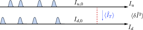
An observable studied in collision experiments [8, 13, 14] (for a schematic setup see Fig. 1) is the generalized Fano factor , defined as the sum of the current noise due to partitioning at the collision QPC and the noise in the incoming currents transmitted through the collision QPC, normalized by the latter [22]. For a fractional quantum Hall edge with equilibrium density fluctuations, the correlation function of an anyon tunneling operator decays like a power law in time, governed by a dynamical exponent . The Fano factor in a symmetric collider setup with two balanced incident anyon beams has been found to be , where a negative is a robust signature of anyonic statistics [22]. This form of the Fano factor applies to cases where and , with the restriction due to the approximation of quasi-particle pulses with vanishing spatial and temporal width made in [22].
However, experiments indicate that the dynamical exponents can deviate from the universal value describing a pristine edge, and may be close to one [12, 13] even for filling . As appears in the expression for the Fano factor, from which one would like to obtain the exchange phase , an uncertainty in leads to an uncertainty in . To reliably determine the exchange phase from experiments, it is therefore necessary to know the Fano factor as a function of outside the range . In addition, previous theory does not apply to the FQH state, where is expected for quasi-particles. The reason is that in the exponential a positive phase has a the same effect as a negative phase , giving rise to a positive due to this ambiguity. Experimentally, small negative Fano factors have been measured [13, 14], and explaining this finding is a challenge for theory.
In this letter, we compute the Fano factor for dynamical exponents for exchange phases and by taking into account a finite width of anyonic pulses in the incident dilute beams. This idea is based on the observation of Schiller et al. [27] that a finite width of quasi-particles allows to correctly compute the Fano factor even for electrons with and . When computing the Fano factor, the time integral describing current cross correlations contains a factor reflecting the equilibrium decay of the correlation function of the anyon tunneling operator. Hence, the integral is dominated by large times for , such that approximating the anyon pulse as zero width is a good approximation. In contrast, for there are relevant contributions from short times where details on the shape of the solitons matter (Fig. 2). The resulting Fano factor for large dynamical exponents is non-universal depending on the width of anyon pulses.
Setup—We consider an anyon collider consisting of chiral edge channels () as schematically illustrated in Fig. 1, which can be realized in FQH systems. Here, the dilute anyon beams impinging on the collision QPC are created by applying a voltage across additional source QPCs (not shown in Fig. 1), allowing tunneling of quasi-particles into the edges with a small tunneling probability , thereby ensuring that the spatial separation between anyons is much larger than their width. The edge states [28] are described as chiral Luttinger liquids [29]. Due to the presence of the collision QPC between the and edge, time-domain interference effects allow the extraction of information about the anyon braiding phase from the tunneling current expectation value and current cross correlations .
In the bosonization formalism, the operator for the tunneling current between upper to the lower edge is given by , with , where is the fractional charge of the anyons, is the tunneling amplitude at the collision QPC, and is the boson field for the anyons on edge . The charge density on the edges is given by . The collision QPC is located at . The equal time commutator is proportional to the fractional charge measured in units of the electron charge , while the equal position commutator contains the dynamical exponent that can be different from and also [30].
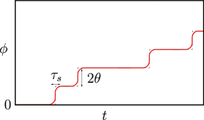
To model the non-equilibrium situation depicted in Fig. 1, we decompose the boson fields into describing the equilibrium quantum fluctuations and a classical non-equilibrium part describing Possionian fluctuations in the quasi-particle number with expectation value [22]. An anyon with exchange phase arriving at time at the collision QPC causes a shift of the non-equilibrium part of the boson field, described by
| (1) |
where we take into account the finite width of the anyon pulses [27] (see Fig. 2). This finite soliton width has previously been neglected by using discrete steps in the boson field, which corresponds to delta peaks in the density.
Current and noise in linear response—The expectation value of the tunneling current is given by . The noise in the tunneling current is obtained as
| (2) |
with the frequency component of its Fourier transform given by .
Under the assumption that the beams are sufficiently dilute, i.e. , we can treat the individual anyons on one edge as independent, allowing to describe them using Poisson statistics. This gives rise to the correlation function
| (3) |
where denotes the non-equilibrium expectation value in absence of the tunneling coupling, and is the equilibrium expectation value of the unperturbed edge with short time cutoff . We defined , where is the current of the dilute beam on edge before the QPC. In Eq. (3), the integral is given by
| (4) |
We used that the real part of the integral is an even function of , while the imaginary part is odd, and the contributions to the exponent of the correlation function for edge is given by ( for and respectively).
By using the expression for the correlation functions Eq. (3) in the current expectation value, we find to leading order in the tunneling amplitude
| (5) |
Similarly, we find that the current noise is given by
| (6) |
In the exponential factors of the current and noise integrands, the transparency of the source QPC
| (7) |
determines how fast the integrands decay. Even in the limit where it seems plausible that tunneling onto edge may be described by a discrete step in the boson field, the short time behavior of the integrals is not accurately approximated. This problem arises for , where the integrals have large short time contributions from the terms.
We denote the ratio of short time cutoff and broadening time as and require . We find below that already for values of - the dependence of current and noise on is negligibly weak.
Fano factor—As an experimentally accessible observable which depends on the braiding phase , we consider the generalized Fano factor
| (8) |
where the denominator is the noise in incoming currents, transmitted through the QPC – a generalization of Johnson-Nyquist noise. The fact that the denominator is defined as a derivative of the current expectation value allows us to focus on the symmetric case, , for which vanishes. It can be shown that the Fano factor only depends on the ratio and has a maximum at [22]. The numerator of the Fano factor contains the sum of the current noise due to partitioning at the QPC and of the transmitted noise. The numerator is given by [22].
For the symmetric case , the denominator of the Fano factor can be expressed as
| (9) |
and the difference between numerator and denominator, i.e., , becomes
| (10) |
These expressions can efficiently be numerically evaluated as they are real and the integral only depend on a single parameter and the reduced time , which allows reusing the results for different values of and .
The full Fano factor in the symmetric case is then given by
| (11) |
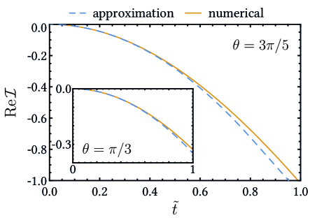
Analytic solution for —Before we discuss the numerical results for as a function of , we first present an approximate analytical solution for , which is close to the experimentally estimated value of the dynamical exponent [12, 13], and show that the Fano factor is non-universal and logarithmically diverging for in this case.
In the limit , the denominator of the Fano factor can be evaluated analytically as the expression in the square brackets of Eq. (5) reduces to the first derivative of a delta distribution and , such that
| (12) |
To evaluate the numerator, we approximate the integral for short times using a Taylor expansion to second order, , and for late times using its asymptotic behavior . We smoothly connect the two approximations at the point , where the asymptotic slope agrees with the slope of the tangent of the quadratic behavior for small times, and obtain for the real part of the integral
| (13) |
In Fig. 3, we show the short time approximation together with the numerically obtained real part of for both and . Using the approximation, we find the Fano factor
| (14) |
with the Euler constant . The logarithmic divergence for indicates that the Fano factor for depends in a significant way on the source QPC transparency .
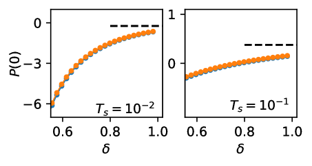

Numerical results for —We numerically compute the Fano factor for anyons with exchange phase . As recent studies [13, 14, 12] indicate that may be realized experimentally, we compute the Fano factor for the symmetric case as a function of (Fig. 4). We find that for a dilution of (panel a), indeed a negative Fano factor is obtained for all , which has a significant dependence on . For even wider solitons with , we find that the Fano factor changes sign as a function of . In Ref. [13], measurements have been performed for and , in agreement with the theoretical finding of for and . In addition, Ref. [14] reports results for dilutions in the range , somewhat outside the the dilute anyon regime discussed here.
Numerical results for — For Laughlin anyons with , we expect to recover the result of a universal Fano factor from Ref. [22] close to . Indeed, we find that the results with finite soliton width show good agreement with the prediction for zero width for (Fig. 5). For larger values of approaching one, the finite soliton width removes the divergence to large negative values, yielding negative Fano factors on the order of for a dilution of , compatible with recent experiments [8, 12, 13, 14].
Discussion—By considering anyon pulses with finite dilution , we find a negative Fano factor in agreement with recent experimental results [14, 13] for anyons with and . However, when further reducing , unphysical jumps in the Fano factor as a function of appear for (not shown in Fig. 4), which are due to a negative tunneling current that cannot be explained by numerical instabilities. In addition, while the results are in overall agreement with experiments, yielding an increasing Fano factor with increasing , the dependence on seems to be somewhat weaker in experiments [13] than predicted theoretically. This could be due to the semi-classical description of non-equilibrium physics, or perhaps related to the -shape of the solitons chosen in our calculation.
Conclusion—Our study reveals the crucial importance of finite soliton widths in analyzing anyon collider (time-domain interference) experiments, especially for exchange phases greater than and dynamical exponents above 1/2. We demonstrate that incorporating a finite soliton width leads to a prediction of negative Fano factors for anyons with exchange phases of , in agreement with recent experimental data. This finding is crucial for accurately interpreting experiments and understanding universal and non-universal contributions to Fano factors in anyonic systems, thereby offering a more comprehensive framework for exploring anyonic statistics in fractional quantum Hall states.
Note added in proof—After completion of this work, we became aware of Ref. [31], which also studies the soliton shape for the description of anyon colliders and finds results consistent with ours.
Acknowledgements.
Acknowledgments: We would thank X.-G. Wen, N. Schiller, G. Fève, and F. Pierre for helpful conversations.References
- Leinaas and Myrheim [1977] J. Leinaas and J. Myrheim, Il nuovo cimento 37, 132 (1977).
- Laughlin [1983] R. B. Laughlin, Physical Review Letters 50, 1395 (1983).
- Halperin [1984] B. I. Halperin, Physical Review Letters 52, 1583 (1984).
- Arovas et al. [1984] D. Arovas, J. R. Schrieffer, and F. Wilczek, Physical review letters 53, 722 (1984).
- Feldman and Halperin [2021] D. E. Feldman and B. I. Halperin, Reports on Progress in Physics 84, 076501 (2021).
- Reznikov et al. [1999] M. Reznikov, R. d. Picciotto, T. Griffiths, M. Heiblum, and V. Umansky, Nature 399, 238 (1999).
- Saminadayar et al. [1997] L. Saminadayar, D. Glattli, Y. Jin, and B. c.-m. Etienne, Physical Review Letters 79, 2526 (1997).
- Bartolomei et al. [2020] H. Bartolomei, M. Kumar, R. Bisognin, A. Marguerite, J.-M. Berroir, E. Bocquillon, B. Placais, A. Cavanna, Q. Dong, U. Gennser, et al., Science 368, 173 (2020).
- Nakamura et al. [2020] J. Nakamura, S. Liang, G. C. Gardner, and M. J. Manfra, Nature Physics 16, 931 (2020).
- Nakamura et al. [2022] J. Nakamura, S. Liang, G. C. Gardner, and M. J. Manfra, Nature Communications 13, 344 (2022).
- Nakamura et al. [2023] J. Nakamura, S. Liang, G. C. Gardner, and M. J. Manfra, Phys. Rev. X 13, 041012 (2023).
- Lee et al. [2023] J.-Y. M. Lee, C. Hong, T. Alkalay, N. Schiller, V. Umansky, M. Heiblum, Y. Oreg, and H.-S. Sim, Nature 617, 277 (2023).
- Ruelle et al. [2023] M. Ruelle, E. Frigerio, J.-M. Berroir, B. Plaçais, J. Rech, A. Cavanna, U. Gennser, Y. Jin, and G. Fève, Physical Review X 13, 011031 (2023).
- Glidic et al. [2023] P. Glidic, O. Maillet, A. Aassime, C. Piquard, A. Cavanna, U. Gennser, Y. Jin, A. Anthore, and F. Pierre, Physical Review X 13, 011030 (2023).
- Safi et al. [2001] I. Safi, P. Devillard, and T. Martin, Physical Review Letters 86, 4628 (2001).
- Vishveshwara [2003] S. Vishveshwara, Physical review letters 91, 196803 (2003).
- Martin [2005] T. Martin, Noise in mesoscopic physics Nanophysics: Coherence and Transport ed H Bouchiat, Y Gefen, S Guéron, G Montambaux and J Dalibard (2005).
- Kim et al. [2005] E.-A. Kim, M. Lawler, S. Vishveshwara, and E. Fradkin, Physical review letters 95, 176402 (2005).
- Vishveshwara and Cooper [2010] S. Vishveshwara and N. Cooper, Physical Review B 81, 201306 (2010).
- Campagnano et al. [2012] G. Campagnano, O. Zilberberg, I. V. Gornyi, D. E. Feldman, A. C. Potter, and Y. Gefen, Physical review letters 109, 106802 (2012).
- Campagnano et al. [2013] G. Campagnano, O. Zilberberg, I. V. Gornyi, and Y. Gefen, Physical Review B 88, 235415 (2013).
- Rosenow et al. [2016] B. Rosenow, I. P. Levkivskyi, and B. I. Halperin, Physical Review Letters 116, 156802 (2016).
- Kim et al. [2006] E.-A. Kim, M. J. Lawler, S. Vishveshwara, and E. Fradkin, Physical Review B 74, 155324 (2006).
- Han et al. [2016] C. Han, J. Park, Y. Gefen, and H.-S. Sim, Nature communications 7, 11131 (2016).
- Lee et al. [2019] B. Lee, C. Han, and H.-S. Sim, Physical Review Letters 123, 016803 (2019).
- Lee et al. [2020] J.-Y. M. Lee, C. Han, and H.-S. Sim, Physical Review Letters 125, 196802 (2020).
- Schiller et al. [2023] N. Schiller, Y. Shapira, A. Stern, and Y. Oreg, Physical Review Letters 131, 186601 (2023).
- Halperin [1982] B. I. Halperin, Physical review B 25, 2185 (1982).
- Wen [1990] X.-G. Wen, Physical Review B 41, 12838 (1990).
- Rosenow and Halperin [2002] B. Rosenow and B. I. Halperin, Phys. Rev. Lett. 88, 096404 (2002).
- Iyer et al. [2023] K. Iyer, F. Ronetti, B. Grémaud, T. Martin, J. Rech, and T. Jonckheere, arXiv preprint arXiv:2311.15094 (2023).