Can Helicity Modulus Be Defined For Boundary Conditions With Finite Twist?

Abstract

We study the response of a two-dimensional classical XY model to a finite (non-infinitesimal) twist of the boundary conditions. We use Monte Carlo simulations to evaluate the free energy difference between periodic and twisted-periodic boundary conditions and find deviations from the expected quadratic dependence on the twist angle. Consequently, the helicity modulus (spin-stiffness) shows a non-trivial dependence on the twist angle. We show that the deviation from the expected behavior arises because of a degeneracy due to the chirality of the spin-waves which leads to an additional entropy contribution in the quasi-long-range ordered phase. We give an improved prescription for the numerical evaluation of the helicity modulus and resolve some open questions related to anti-periodic boundary conditions. We also discuss applications to discrete spin systems and some experimental scenarios where boundary conditions with finite twist are necessary.

1 Introduction

The study of magnetic systems with the help of spin models such as the Ising or Heisenberg models has resulted in tremendous progress in condensed matter physics. For ferromagnetic systems in the thermodynamic limit, surface energies are negligible, and the choice of boundary conditions can be considered unimportant. On the other hand, in disordered systems such as spin glasses, effects of various boundary conditions have been a topic of active interest [1, 2, 3]. In the presence of long-range interactions in an Ising spin system, different choices of boundary condition lead to seemingly different thermodynamic behaviors. By choosing artificial coupling-dependent boundary condition, an uncountable number of exotic spin states of the ground state can be generated at any temperature, whereas free boundary conditions, which are considered physical, do not generate the same effect [4]. In the XY or Heisenberg spin glasses, small rotations at the boundary are expected to yield non-smooth changes in ground state [5]. Thermodynamic Casimir forces, which arise due to the confinement of critical order parameter fluctuations, were found to be affected by the angle between surface fields [6, 7]. However, to the best of our knowledge, a detailed investigation of the boundary dependence in continuous spin systems, similar to the above studies of Ising models, is still missing.

In this paper, we consider the seemingly simpler but surprisingly complex effects of a finite (non-infinitesimal) twist of the boundary conditions on a ferromagnetic XY system. Arguments put forward by Brown and Ciftan [8] in the context of the three-dimensional Heisenberg model suggest that the mixing of states with different chirality plays an important role and affects the observed helicity modulus. However, a quantitative understanding of this effect and its origins has not been achieved yet. We therefore study this question in detail for the two-dimensional classical XY model by means of large-scale Monte Carlo simulations. We find that the free energy cost of a non-infinitesimal twist in the boundary condition in the quasi long-range ordered (QLRO) low-temperature phase deviates from the expected quadratic dependence on the twist angle. Mixing of states with opposite chirality provides an extra entropy contribution which takes the value $\ln(2)$ (in units in which $k_{B}=1$) for a $\pi-$twist. Beyond their intrinsic interest, our results potentially apply to experiments aimed at detecting the Berezinskii–Kosterlitz–Thouless (BKT) transition [9, 10]. They are also important for systems with discrete $Z(N)$ (clock) order parameter symmetry where any twist in the boundary conditions is necessarily non-infinitesimal. In addition, our findings enable novel numerical algorithms for computing the helicity modulus in simulations.

Our paper is organized as follows. In section 2, we introduce the Hamiltonian under various boundary conditions, and we discuss the boundary condition dependence of the free energy. Section 3 contains the details of numerical simulations. In section 4, we present our results for the helicity modulus evaluated for a finite twist in the boundary condition, and we perform a detailed analysis of the twist dependence of thermodynamic observables. We conclude in section 5.

2 The Model

We are interested in the classical XY model, a system of planar spins described by the Hamiltonian

$$H=-J\sum_{<ij>}\mathbf{S}_{i}\cdot\mathbf{S}_{j}=-J\sum_{<ij>}\cos(\phi_{i}-\phi_{j})~{}.$$ (1)

Here, $J>0$ denotes the ferromagnetic exchange interaction (which will be set to unity in the simulations), the sum is over pairs of nearest neighbors on a $d$-dimensional hypercubic lattice, and $\mathbf{S}=(S_{x},S_{y})$ is a two-component unit vector. Equivalently, the XY spins can be represented by their phases, $\phi$ defined via $S_{x}=\cos\phi,~{}S_{y}=\sin\phi$. Twisted boundary conditions can be implemented by fixing the spins at two opposite boundaries at specific orientations (phases) with a fixed angle $\Theta$ between them. Alternatively, we consider the Hamiltonian (1) with periodic boundary conditions and modify the interactions across one of the boundaries to introduce the twist. This is achieved by replacing the interaction terms across the chosen boundary by $-J\cos(\phi_{i}-\phi_{j}-\Theta)$. We call these boundary conditions twisted-periodic, and the usual periodic boundary conditions are recovered for $\Theta=0$.

The phase diagram of the classical XY model is well-understood. Long-range order is impossible in one and two dimensions at any nonzero temperature due to the Mermin-Wagner theorem [11]. In three and higher dimensions, there is a phase transition between a paramagnetic high-temperature phase and a ferromagnetic low-temperature phase. The two-dimensional XY model is special because the system undergoes a BKT phase transition into a quasi long-range ordered low-temperature phase.

In a long-range ordered or quasi long-range ordered phase, a twist in the boundary conditions increases the system’s free energy. The system can lower its free energy by distributing the total twist (angular difference) $\Theta$ over the entire sample, i.e., by gradually changing the average orientation of the spins in the bulk. For a system of linear size $L$, the lowest free energy is expected when the average phase changes by $\Theta/L$ between neighboring sites (in the direction the twist is applied). For large $L$, this local phase change is small, and free energy can be expanded in powers of $\Theta/L$. As the free energy difference $\Delta F$ between the twisted and untwisted systems must be an even function of $\Theta$, it takes the form

$$\Delta F=F_{\Theta}-F_{0}=\frac{\rho_{s}}{2}\left(\frac{\Theta}{L}\right)^{2}L^{d}$$ (2)

to quadratic order in $\Theta/L$. This relation can be understood as a definition of the helicity modulus (or spin stiffness) $\rho_{s}$,

$$\rho_{s}(\Theta)=\frac{2\Delta F}{\Theta^{2}}L^{2-d}.$$ (3)

In the limit of an infinitesimal twist, the helicity modulus can be rewritten as $\rho_{s}(\Theta\rightarrow 0)=\left({\partial^{2}F}/{\partial\Theta^{2}}\right)_{\Theta=0}L^{2-d}$. By treating the twist angle $\Theta$ as a parameter in the Hamiltonian, the partial derivative $\left({\partial^{2}F}/{\partial\Theta^{2}}\right)_{\Theta=0}$ can be expressed in terms of appropriate thermodynamic averages in the untwisted system. This leads to the formula [12]

$$\left(\frac{\partial^{2}F}{\partial\Theta^{2}}\right)_{\Theta=0}= \frac{1}{L^{2-d}}\sum_{<ij>}J\left\langle\cos(\phi_{i}-\phi_{j})\right\rangle_{\Theta=0}(x_{i}-x_{j})^{2}$$ (4)

$$-\frac{\beta}{L^{2-d}}\left\langle\left\{\sum_{<ij>}J~{}\sin(\phi_{i}-\phi_{j})(x_{i}-x_{j})\right\}^{2}\right\rangle_{\Theta=0}.$$ (5)

where $x_{i}$ is the coordinate of site $i$ in the twisted direction.

As the paramagnetic phase is insensitive to the boundary conditions, the free energy difference decays exponentially with system size, $\Delta F\sim e^{-L/\xi}$ , where $\xi$ is the correlation length. This implies $\rho_{s}=0$ in the paramagnetic phase in the thermodynamic limit. In contrast, $\Delta F$ is expected to scale as $L^{d-2}$ in an ordered or quasi long-range ordered phase, and the helicity modulus is finite. In two dimensions, $\rho_{s}$ is known to have an universal jump at the BKT phase transition. For $d>2$, $\rho_{s}$ vanishes continuously at $T_{c}$, governed by critical behavior of the phase transition. In the rest of the paper, we focus on two dimensions, but we will comment on higher dimensions in the concluding section.

3 Numerical Simulations

We perform large-scale Monte Carlo simulations to evaluate the free energy difference between systems with periodic and twisted-periodic boundary conditions. The free energy cannot be measured directly in a standard Monte Carlo simulation. Instead, it can be evaluated explicitly by integrating the internal energy $U=\langle H\rangle$ over the inverse temperature $\beta=1/T$,

$$F(T)=F(T_{0})+T\int_{\beta_{0}}^{\beta}d\beta^{\prime}U(\beta^{\prime})~{}.$$ (6)

We choose the starting temperature $T_{0}$ sufficiently high (well above the BKT transition) such that the free energies of the twisted and untwisted systems agree with each other within the statistical errors. This ensures that $F(T_{0})$ drops out of the free energy difference (2). We note that there are alternative approaches that allow one to directly measure the free energy difference between different boundary conditions in a simulation. This is achieved by including appropriate boundary terms as dynamical variables in the Monte Carlo scheme (see, e.g., Refs. [13, 14]). The challenge in these approaches is to ensure a sufficiently rapid relaxation of the boundary variables, especially in the absence of cluster algorithms.

Our simulations employ both the single spin-flip Metropolis algorithm [15, 16] and the Wolff cluster-flip algorithm [17]. For systems with periodic boundary conditions, the efficient Wolff algorithm greatly reduces critical slowing down. Thus, a full MC sweep consists of one Metropolis sweep followed by one Wolff sweep for the case of periodic boundary conditions. However, for twisted-periodic boundary conditions with twist angle $0<\Theta<\pi$, the Wolff algorithm cannot be employed. This stems from the fact that the angle between two spins of a Wolff cluster is not preserved (but rather changes sign) when the cluster is flipped. Consequently, the cluster flip changes the energy of a twisted bond inside the cluster, invalidating the algorithm. In the case of twisted-periodic boundary conditions with $0<\Theta<\pi$, we therefore only employ Metropolis sweeps. For a twist angle of exactly $\pi$, the twisted bonds effectively become antiferromagnetic as $\cos(\Delta\phi-\pi)=-\cos(\Delta\phi)$. The energy of an antiferromagnetic bond is invariant under a sign change of $\Delta\phi$, and the Wolff algorithm can be used.

To facilitate the numerical integration (6) for the free energy, we initiate the simulations at the highest temperature $T_{0}$ (using a “hot” start, i.e., all spins are randomly oriented at the beginning of the simulation). The temperature is then reduced in small steps $dT$ until the desired final temperature is reached. Most production simulations started from $T_{0}=30$, much higher than the BKT transition temperature of $T_{c}=0.89290(5)$ [18]. The temperature step $dT$ is gradually decreased from $dT=0.5$ at $T_{0}$ to $dT=0.02$ in the transition region and below. To check how sensitive the free energy difference $\Delta F$ is to these parameters, we performed tests with $T_{0}$ as high as 90 and $dT$ as low as 0.01. The free energy differences resulting from these test calculations agreed with the production results within their statistical errors.

For periodic boundary conditions, we perform up to $2000$ full equilibration sweeps (each consisting of a Metropolis sweep followed by a Wolff sweep) and up to $8000$ full measurement sweeps at each temperature step. For twisted-periodic boundary conditions, we perform up to about $80\,000$ (Metropolis only) equilibration sweeps and up to about $160\,000$ measurement sweeps. (As usual, the quality of the equilibration was confirmed by comparing the results of hot and cold starts.) We simulate systems of linear sizes up to $L^{2}=80^{2}$ and average the results over about $5000$ samples. Each sample is subjected to periodic and twisted-periodic boundary conditions, and the resulting free energies are compared to evaluate the helicity modulus (3).

We use an ensemble method (see, e.g., Ref. [19]) to estimate the error of the free energy. We generate a large ensemble of synthetic internal energy curves ${U_{i}(T)=U(T)+r(T)~{}\Delta U(T)}$, where $\Delta U$ is the statistical error obtained from Monte Carlo and $r(T)$ is a random number chosen from a normal distribution of unit variance. Integrating these curves via (6) generates an ensemble of free energies $F_{i}$. Mean and standard deviation of this ensemble are then propagated through (3) to find the helicity modulus and the associated error.

4 Results

We now turn to our results for the response of the two-dimensional XY model to various twists in the boundary conditions. Figure 1 shows the helicity modulus $\rho_{s}$ as a function of temperature for three different cases, viz., an infinitesimal twist, a twist of $\Theta=\pi/6$, and a twist of $\Theta=\pi$.

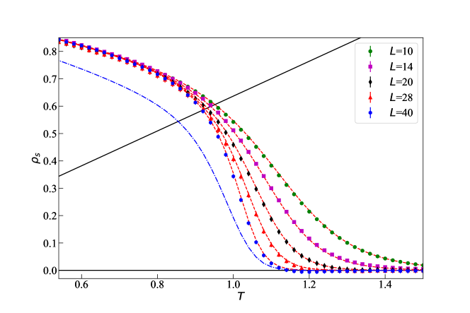
Figure 1: Helicity modulus $\rho_{s}$ as a function of temperature $T$ for different system sizes $L$. The filled symbols show $\rho_{s}$ for a twist of $\Theta=\pi/6$, obtained from the definition (3) using the free energies (6). The dotted lines denote $\rho_{s}$ for an infinitesimal twist measured in the untwisted system via eq. (5). The helicity modulus values for these two cases agree within their statistical errors (which are comparable to or smaller than the symbol sizes). The straight solid line corresponds to $\rho_{s}=2T/\pi$, it intersects the stiffness curves at temperatures $T^{*}(L)$. The critical temperature $T_{c}$ is obtained by extrapolating $T^{*}(L)$ to the thermodynamic limit according to eq. (7). This extrapolation gives $T_{c}=0.891(7)$. In contrast, the helicity modulus values for a twist of $\Theta=\pi$, shown as dash-dotted line for $L=40$, are significantly lower than the other data.

For the infinitesimal twist, $\rho_{s}$ is measured in the untwisted system via eq. (5). For the finite twists, $\rho_{s}$ is obtained from the free energy difference between simulations with twisted and untwisted boundary conditions, as explained in Sec. 3. The resulting $\rho_{s}$ values for the infinitesimal twist and $\Theta=\pi/6$ agree within their statistical errors, giving us additional confidence in our numerical approach.

The helicity modulus curves can be used to find the critical temperature. In the thermodynamic limit, $\rho_{s}$ vanishes in the disordered phase whereas it is nonzero in the quasi long-range ordered phase. The BKT transition is marked by a universal jump in $\rho_{s}$. Using the Kosterlitz-Nelson relation, $T_{c}$ can be identified by the intersection of the infinite-system $\rho_{s}$ vs. $T$ curve with a straight line of slope $2/\pi$ [20]. As the correlation length increases exponentially for $T\rightarrow T_{c}$ at a BKT transition, finite-size corrections take a logarithmic form. Thus, $T_{c}$ is found by extrapolating $T^{*}(L)$, the temperature at which the $\rho_{s}$ vs. $T$ curve for size $L$ intersects the line of slope $2/\pi$, according to

$$T^{*}(L)=T_{c}+\frac{A}{\ln^{2}(bL)}$$ (7)

where $A,b$ are non-universal fitting parameters. We find $T_{c}=0.891(7)$ from twisted boundary conditions with $\Theta=\pi/6$, which agrees with high-accuracy results in the literature [18, 21, 22, 23].

We also studied a twist of $\Theta=\pi$. Unexpectedly, the resulting helicity modulus values are significantly below the values for smaller $\Theta$, as shown in Fig. 1. It is worth emphasizing that this happens even though the layer-to-layer twist $\Theta/L$ remains small compared to unity, justifying the expansion that leads to eq. (2). What is the reason for this surprising discrepancy? Arguments put forward in Ref. [8] suggest that the chirality of the twist plays an important role.

So far we have considered thermodynamic states that fulfill the global twist $\Theta$ in, say, clockwise direction by introducing an average clockwise twist of $\Theta/L$ between neighboring layers. However, the same global twist can be achieved by a counter-clockwise twist with local angle of $(2\pi-\Theta)/L$ between consecutive layers. At low temperatures, the additional free energy for a twist in the “wrong” direction is much larger than $k_{B}T$. Therefore, this state is exponentially suppressed. Local twist angles corresponding to higher winding numbers can also be ruled out using the same argument. However, with increasing temperature, states of both chiralities (and higher winding numbers) will be mixed, leading to an extra entropic contribution to the free energy. Importantly, $\Theta=\pi$ is a special case that allows the mixing of opposite chiralities even at $T=0$. Let us now study this idea quantitatively.

According to eq. (2), we expect the free energy difference between the twisted and untwisted systems to behave as $\Delta F\propto\Theta^{2}$, at least as long as higher-order terms in $\Theta/L$ can be neglected. We have studied the $\Theta$ dependence of $\Delta F$ systematically at various temperatures in the quasi long-range ordered phase close to $T_{c}$; the results are presented in Fig. 2.

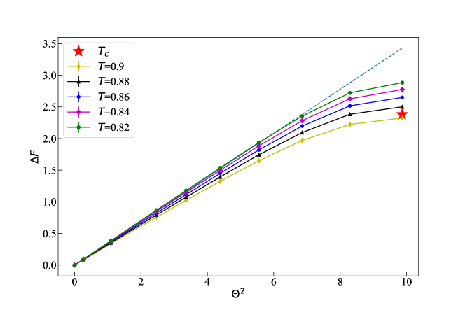
Figure 2: Free energy difference $\Delta F$ vs. squared twist angle $\Theta^{2}$ for size $L=40$ and several temperatures close to $T_{c}$. The dotted line shows a fit of $\Delta F$ for $T=0.82$ to a quadratic $\Theta$ dependence in the range $0\leq\Theta^{2}\leq(2\pi/3)^{2}$. $\Delta F$ at $T_{c}\approx 0.893$, obtained using eq. (8) is marked by the star symbol.

The figure shows that $\Delta F$ follows the quadratic $\Theta$ dependence up to about $\Theta=2\pi/3$ but significant deviations are observed for larger twist angles. The special case of anti-periodic boundary conditions ($\Theta=\pi$) right at the BKT transition temperature was studied by Hasenbusch [24, 25]. He derived an expression for the ratio of the partition functions with periodic and antiperiodic boundary conditions in the two-dimensional XY model. It includes the leading finite-size corrections and reads

$$\frac{Z_{\Theta=\pi}}{Z_{\Theta=0}}=0.08643(1)-\frac{0.1358(1)}{\ln(L)+C}~{},$$ (8)

where the constant $C$ approximately captures contributions from higher order terms. For the purpose of comparing with our Monte Carlo results, we set $C=4.3$ as in Ref. [24]. The free energy difference $\Delta F$ resulting from this formula agrees well with our data, see Fig. 2.

We attribute the deviation of $\Delta F$ from the quadratic $\Theta$ dependence to the mixing of states of opposite chirality which becomes more pronounced as $\Theta$ approaches $\pi$. To quantify this mechanism, we determine the excess free energy due to the mixing. To this end, we first fit a quadratic function to $\Delta F(\Theta)$ in the range $0\leq\Theta\leq 2\pi/3$ (separately for each system size). Denoting the fit function by $\Delta F_{fit}(L,T,\Theta)$, we define the excess free energy $\delta\Delta F$ at twist angle $\pi$ as the difference between $\Delta F_{fit}(L,T,\pi)$ and the $\Delta F_{MC}(L,T,\pi)$ obtained from MC,

$$\delta\Delta F(L,T,\pi)=\Delta F_{fit}(L,T,\pi)-\Delta F_{MC}(L,T,\pi).$$ (9)

In other words, $\Delta F_{fit}$ is the free energy cost of the twist expected if only states of one chirality contribute, whereas $\delta\Delta F$ captures the additional free energy due to chirality mixing.

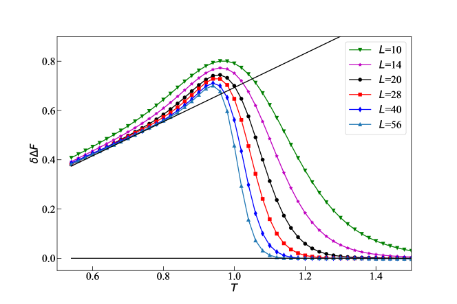
Figure 3: Excess free energy $\delta\Delta F(L,T,\pi)$ defined in eq. (9) for a twist angle of $\pi$ as a function of temperature $T$ for different system sizes. The solid line represents the function $T\ln(2)$.

Figure 3 shows the excess free energy $\delta\Delta F$ for twist angle $\pi$ as a function of temperature $T$ for various system sizes. For temperatures $T>T_{c}$, in the disordered phase, $\delta\Delta F$ decreases with increasing system size and appears to vanish in the thermodynamic limit. For temperatures $T<T_{c}$, in contrast, $\delta\Delta F$ approaches a nonzero limit for $L\to\infty$. This infinite-system limit of $\delta\Delta F$ follows the function $T\ln(2)$ as temperature goes to zero .

As the excess free energy is expected to be entropic in nature, we define $\delta S=\delta\Delta F/T$ as the excess entropy due to the mixing of chiralities. Our numerical results for the excess entropy are presented in Fig. 4.

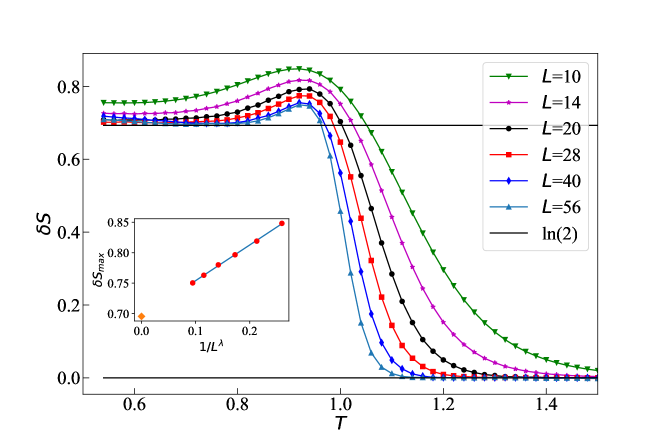
Figure 4: Excess entropy $\delta S$ due to the mixing of chiralities vs. temperature $T$ for different system sizes. The solid horizontal line corresponds to $\delta S=\ln(2)$. The inset shows the extrapolation of the maximum value of each $\delta S$ vs. $T$ curve to infinite system size. The extrapolation gives $\delta S_{max}(L=\infty)=0.69(1)$ and agrees with $\ln(2)$.

The figure shows that $\delta S$ approaches zero with increasing system size for high temperatures while it appears to approach a constant for low temperatures. In fact, the figure suggests that $\delta S$ approaches a step function in the thermodynamic limit. To determine the step height and position, we extrapolate the peak value $\delta S_{max}$ of the $\delta S$ vs. $T$ curves using,

$$\delta S_{max}(L)=\delta S_{max}(\infty)+aL^{-\lambda}$$ (10)

where $a,\lambda$ are fitting parameters. (We determine $\delta S_{max}$ as an extremum of a quadratic curve fitted in the vicinity of the peak.) The extrapolation is shown in the inset of Fig. 4 and yields $\delta S_{\infty}=0.69(1)\approx\ln(2)$, in agreement with the expectation of contributions from two degenerate states. Additionally, an extrapolation of the temperature at which the $\delta S$ vs. $T$ curves cross the $\delta S=\ln(2)$ line matches with $T_{c}$ within the error bars. Thus, our numerical data extrapolate to $\delta S=\ln(2)\Theta(T_{c}-T)$ where $\Theta$ is the Heavyside step function. We note that the arguments predicting the excess $\ln(2)$ entropy due to the chirality mixing do not include states with higher winding numbers. These states are known to renormalize the helicity modulus in two dimensions [26, 22], but the effect is tiny and only visible in high-accuracy simulations beyond our numerical precision.

The excess entropy due to the chirality mixing reduces the free energy cost of a $\pi$ twist by $T\ln(2)$. Consequently, the helicity modulus $\rho_{s}(\pi)$ computed directly from eq. (3) is reduced by $2\ln(2)T/\pi^{2}$. This explains the observation in Fig. 1 of a lower helicity modulus for the $\pi$ twist. Consequently, if one wishes find the critical temperature from simulations employing a $\pi$ twist (i.e., anti-periodic boundary conditions), the reduction of $\rho_{s}$ has to be accounted for. This can be achieved by modifying the Kosterlitz-Nelson relation by changing the slope of the line crossing the $\rho_{s}$ curves from $2/\pi$ to $2/\pi-2~{}\ln(2)/\pi^{2}$. The resulting analysis is presented in Fig. 5 which shows the helicity modulus for a $\pi$ twist as a function of temperature for different system sizes.

Figure 5: Helicity modulus $\rho_{s}$ for a twist of $\Theta=\pi$ (anti-periodic boundary conditions). The inset shows the intersection temperatures $T^{*}$ of the helicity modulus curves with the modified Kosterlitz-Nelson line of slope $2/\pi-2~{}\ln(2)/\pi^{2}$. An extrapolation according to eq. (7) yields $T_{c}=0.897(2)$.

To find $T_{c}$ we extrapolate, using eq. (7), the intersection temperature of the $\rho_{s}$ curves with a line of modified slope, and obtain $T_{c}=0.897(2)$. This is in reasonable agreement with the literature value [22].

5 Conclusion

To summarize, in this paper we have studied the effects of finite (non-infinitesimal) twists in the boundary conditions on a two-dimensional classical ferromagnetic XY model. The system’s response to the twist has been studied by direct evaluation of the free energy by means of Monte Carlo simulations. We have found that in the quasi long-range ordered phase, the free energy cost of a non-infinitesimal twist deviates from the expected quadratic dependence on the twist angle. In the case of a $\pi$ twist (anti-periodic boundary conditions), the mixing of states of opposite chiralities causes an excess entropy contribution of $\ln(2)$ which reduces the observed helicity modulus compared to the value for an infinitesimal twist. This analysis has allowed us to accurately determine the helicity modulus from simulations with anti-periodic boundary conditions. A modified Kosterlitz-Nelson relation can be used to determine the critical temperature.

The present paper has focused on two dimensions. Two dimensions are a special case because the free energy cost of a twist is independent of system size, see eq. (2). Thus, the excess entropy discussed above makes a non-negligible contribution even in the thermodynamic limit. In a higher dimensional XY model, the excess entropy would still take the value ln(2) for a $\pi$ twist. However, its contribution to the helicity modulus, $2\ln(2)L^{2-d}/\pi^{2}$, would vanish in the thermodynamic limit.

Our work also relates to some of the questions raised by Brown and Ciftan [8]. They studied the effects of twisted-periodic and anti-periodic boundary conditions on a three-dimensional classical Heisenberg model and discussed the notion of mixing states of different chiralities in response to twisted-periodic boundary conditions. However, they analyzed the internal energy cost of the twist rather than the free energy cost. The authors report deviations from a quadratic twist angle dependence of the internal energy cost somewhat similar to what we find for $\Delta F$, but the magnitude of the deviation in their case is much larger than $T\ln(2)$. Moreover, the internal energy cost (as opposed to $\Delta F$) is not expected to contain the entropy due to the mixing of chiralities. This suggests that the deviations from a quadratic twist angle dependence of the internal energy cost in Ref. [8] have a different origin. Specifically, Heisenberg spins can reduce the energy cost of twisted-periodic boundary conditions by tilting out of the plane in which the twist is applied. In contrast, they cannot avoid antiperiodic boundary conditions, in agreement with the fact that the energy cost of anti-periodic boundary conditions in Ref. [8] is much larger that of even the largest twist angles. A quantitative analysis of the effects of twisted-periodic boundary conditions in the Heisenberg case remains a task for the future.

Our results have potential implications for experiments proposed to detect the BKT phase transitions [27], in which anti-parallel external fields would be used to study charge-current cross correlations. Moreover, in discrete spin systems such as the $q-$state clock model [28], twists are necessarily non-infinitesimal, and corrections to the infinitesimal-twist helicity modulus must be considered.

It is also interesting to ask what implications our findings have in the context of the quantum-to-classical mapping. The partition function of a quantum system in $d$ dimensions can often be mapped onto that of a classical system in $d+1$ dimensions. How does the extra entropy contribution in the classical Hamiltonian with $\pi$-twisted boundary conditions manifest itself in the ground state of the corresponding quantum system?

6 Acknowledgements

The authors acknowledge support from the National Science Foundation under grant nos. DMR-1506152, DMR-1828489, OAC-1919789. Simulations were performed on the Foundry and Pegasus Clusters at Missouri University of Science and Technology.

7 References

References

- [1] Banavar J R, Cieplak M and Cieplak M Z 1982 Influence of boundary conditions on random unfrustrated magnetic systems Physical Review B 26 2482
- [2] Newman C M and Stein D L 1992 Multiple states and thermodynamic limits in short-ranged ising spin-glass models Physical Review B 46 973
- [3] Endo E O, van Enter A C and Le Ny A 2021 The roles of random boundary conditions in spin systems In and Out of Equilibrium 3: Celebrating Vladas Sidoravicius ed Vares M E, Fernandez R, Fontes L R and Newman C M (Springer) pp 371–381
- [4] Gandolfi A, Newman C M and Stein D L 1993 Exotic states in long-range spin glasses Communications in Mathematical Physics 157 371–387
- [5] Fisher D S and Huse D A 1988 Equilibrium behavior of the spin-glass ordered phase Physical Review B 38 386–411
- [6] Bergknoff J, Dantchev D and Rudnick J 2011 Casimir force in the rotor model with twisted boundary conditions Physical Review E 84 041134
- [7] Dantchev D and Rudnick J 2017 Manipulation and amplification of the casimir force through surface fields using helicity Physical Review E 95 042120
- [8] Brown R G and Ciftan M 2006 Critical behavior of the helicity modulus for the classical Heisenberg model Physical Review B 74(22) 224413
- [9] Berezinskii V L 1971 Sov. Phys. JETP 32 493
- [10] Kosterlitz J M and Thouless D J 1973 J. Phys. C 6 1181
- [11] Mermin N D and Wagner H 1966 Absence of ferromagnetism or antiferromagnetism in one- or two-dimensional isotropic Heisenberg models Phys. Rev. Lett. 17(22) 1133–1136
- [12] Teitel S and Jayaprakash C 1983 Phase transtions in frustrated two-dimensional models Physical Review B 27(1) 598–601
- [13] Hasenbusch M 1993 Direct Monte Carlo measurement of the surface tension in ising models Journal de Physique I 3(3) 753–765
- [14] Hukushima K 1999 Domain-wall free energy of spin-glass models: Numerical method and boundary conditions Phys. Rev. E 60(4) 3606–3613
- [15] Metropolis N and Ulam S 1949 The Monte Carlo method Journal of the American statistical association 44 335–341
- [16] Metropolis N, Rosenbluth A W, Rosenbluth M N, Teller A H and Teller E 1953 Equation of state calculations by fast computing machines J. Chem. Phys. 21 1087–1092
- [17] Wolff U 1989 Collective Monte Carlo updating for spin systems Physical Review Letters 62 361
- [18] Ueda A and Oshikawa M 2021 Resolving the berezinskii-kosterlitz-thouless transition in the two-dimensional xy model with tensor-network-based level spectroscopy Physical Review B 104 165132
- [19] Khairnar G, Lerch C and Vojta T 2021 Phase boundary near a magnetic percolation transition European Physical Journal B 94 1–8
- [20] Nelson D R and Kosterlitz J 1977 Universal jump in the superfluid density of two-dimensional superfluids Physical Review Letters 39 1201
- [21] Hasenbusch M and Pinn K 1997 Computing the roughening transition of ising and solid-on-solid models by bcsos model matching Journal of Physics A: Mathematical and General 30 63
- [22] Hsieh Y D, Kao Y J and Sandvik A W 2013 Finite-size scaling method for the Berezinskii–Kosterlitz–Thouless transition Journal of Statistical Mechanics: Theory and Experiment 2013 P09001
- [23] Jha R G 2020 Critical analysis of two-dimensional classical XY model Journal of Statistical Mechanics 2020 083203
- [24] Hasenbusch M 2009 The kosterlitz–thouless transition in thin films: a monte carlo study of three-dimensional lattice models Journal of Statistical Mechanics: Theory and Experiment 2009 P02005
- [25] Hasenbusch M 2005 The two-dimensional xy model at the transition temperature: a high-precision monte carlo study Journal of Physics A: Mathematical and General 38 5869
- [26] Prokof’ev N V and Svistunov B V 2000 Two definitions of superfluid density Phys. Rev. B 61(17) 11282–11284
- [27] Troncoso R E, Brataas A and Sudbø A 2020 Fingerprints of universal spin-stiffness jump in two-dimensional ferromagnets Physical Review Letters 125 237204
- [28] Kumano Y, Hukushima K, Tomita Y and Oshikawa M 2013 Response to a twist in systems with z p symmetry: The two-dimensional p-state clock model Physical Review B 88 104427