Parameter Inference for Hypo-Elliptic Diffusions under a Weak Design Condition

Abstract

We address the problem of parameter estimation for degenerate diffusion processes defined via the solution of Stochastic Differential Equations (SDEs) with diffusion matrix that is not full-rank. For this class of hypo-elliptic diffusions recent works have proposed contrast estimators that are asymptotically normal, provided that the step-size in-between observations $\displaystyle\Delta=\Delta_{n}$ and their total number $\displaystyle n$ satisfy $\displaystyle n\to\infty$, $\displaystyle n\Delta_{n}\to\infty$, $\displaystyle\Delta_{n}\to 0$, and additionally $\displaystyle\Delta_{n}=o(n^{-1/2})$. This latter restriction places a requirement for a so-called rapidly increasing experimental design. In this paper, we overcome this limitation and develop a general contrast estimator satisfying asymptotic normality under the weaker design condition $\displaystyle\Delta_{n}=o(n^{-1/p})$ for general $\displaystyle p\geq 2$. Such a result has been obtained for elliptic SDEs in the literature, but its derivation in a hypo-elliptic setting is highly non-trivial. We provide numerical results to illustrate the advantages of the developed theory.

Keywords: Stochastic Differential Equation; hypo-elliptic diffusion; high-frequency observations; experimental design of observations.

1 Introduction

We consider the problem of parameter inference for multivariate Stochastic Differential Equations (SDEs) determined via a degenerate diffusion matrix. Let $\displaystyle(\Omega,\mathcal{F},\{\mathcal{F}_{t}\}_{t\geq 0},\mathbb{P})$ be a filtered probability space and let $\displaystyle W=(W_{t}^{1},\ldots,W_{t}^{d})$, $\displaystyle t\geq 0$, be the $\displaystyle d$-dimensional standard Brownian motion, $\displaystyle d\geq 1$, defined on such a space. We introduce $\displaystyle N$-dimensional SDE models, $\displaystyle N\geq 1$, of the following general form:

$$\displaystyle dX_{t}=\mu(X_{t},\theta)dt+\sum_{j=1}^{d}A_{j}(X_{t},\theta)dW_{t}^{j},\qquad X_{0}=x\in\mathbb{R}^{N},$$ (1.1)

with $\displaystyle\mu,A_{j}(\cdot,\theta):\mathbb{R}^{N}\to\mathbb{R}^{N}$, $\displaystyle 1\leq j\leq d$, for parameter $\displaystyle\theta$. This work focuses on the case where the diffusion matrix $\displaystyle A=[A_{1},\ldots,A_{d}]$ is not of full-rank, i.e. the matrix $\displaystyle a=AA^{\top}$ is not positive definite. Also, the law of the solution to (1.1) is assumed to be absolutely continuous with respect to (w.r.t.) the Lebesgue measure. Such models are referred to as hypo-elliptic diffusions and constitute an important class of continuous-time Markovian processes, used in a wide range of applications. E.g., this model class includes the (underdamped) Langevin equation, the Synaptic-Conductance model (Ditlevsen and Samson, 2019), the $\displaystyle\mathrm{NLCAR}(p)$ model (Tsai and Chan, 2000; Stramer and Roberts, 2007), the Jansen-Rit neural mass model (Buckwar et al., 2020), the Susceptible-Infected-Recovered (SIR) epidemiological model (Dureau et al., 2013; Spannaus et al., 2022) and the quasi-Markovian generalised Langevin equations ($\displaystyle q$-GLE) (Vroylandt et al., 2022). We investigate two (sub-)classes of hypo-elliptic SDEs which cover a wide range of models, including the ones mentioned in the above examples. The first model class is specified via the following SDE:

$$\displaystyle\begin{aligned} dX_{t}&=\begin{bmatrix}dX_{S,t}\\[5.69046pt] dX_{R,t}\end{bmatrix}=\begin{bmatrix}\mu_{S}(X_{t},\beta_{S})\\[5.69046pt] \mu_{R}(X_{t},\beta_{R})\end{bmatrix}dt+\sum_{j=1}^{d}\begin{bmatrix}\mathbf{0}_{N_{S}}\\[5.69046pt] A_{R,j}(X_{t},\sigma)\end{bmatrix}dW_{t}^{j},\qquad X_{0}=x\equiv\begin{bmatrix}x_{S}\\ x_{R}\end{bmatrix}\in\mathbb{R}^{N}.\end{aligned}$$ (Hypo-I)

The involved drift functions and diffusion coefficients are specified as follows:

$$\displaystyle\mu_{S}:\mathbb{R}^{N}\times\Theta_{\beta_{S}}\to\mathbb{R}^{N_{S}},\quad\mu_{R}:\mathbb{R}^{N}\times\Theta_{\beta_{R}}\to\mathbb{R}^{N_{R}},\qquad A_{R,j}:\mathbb{R}^{N}\times\Theta_{\sigma}\to\mathbb{R}^{N_{R}},\quad 1\leq j\leq d,$$

for positive integers $\displaystyle N_{S},N_{R}$ such that $\displaystyle N=N_{S}+N_{R}$. Here, the unknown parameter vector is

$$\theta=(\beta_{S},\beta_{R},\sigma)\in\Theta=\Theta_{\beta_{S}}\times\Theta_{\beta_{R}}\times\Theta_{\sigma}\subseteq\mathbb{R}^{N_{\beta_{S}}}\times\mathbb{R}^{N_{\beta_{R}}}\times\mathbb{R}^{N_{\sigma}},$$

for positive integers $\displaystyle N_{\beta_{S}},\,N_{\beta_{R}},\,N_{\sigma}$ satisfying $\displaystyle N_{\beta_{S}}+N_{\beta_{R}}+N_{\sigma}=N_{\theta}$. The parameter space $\displaystyle\Theta$ is assumed to be a compact subset of $\displaystyle\mathbb{R}^{N_{\theta}}$. We will later on place a condition on (Hypo-I), related to the so-called Hörmander’s condition, so that indeed such an SDE gives rise to a hypo-elliptic process, i.e. finite-time transition distributions of the SDE admit a Lebesgue density. In brief, the condition will guarantee that randomness from the rough component $\displaystyle X_{R,t}$ propagates into the smooth component $\displaystyle X_{S,t}$ via the drift function $\displaystyle\mu_{S}$. The second hypo-elliptic model class we treat in this work is specified via the following SDE:

$$\displaystyle\begin{aligned} dX_{t}&=\begin{bmatrix}dX_{S_{1},t}\\[5.69046pt] dX_{S_{2},t}\\[5.69046pt] dX_{R,t}\end{bmatrix}=\begin{bmatrix}\mu_{S_{1}}(X_{S,t},\beta_{S_{1}})\\[5.69046pt] \mu_{S_{2}}(X_{t},\beta_{S_{2}})\\[5.69046pt] \mu_{R}(X_{t},\beta_{R})\end{bmatrix}dt+\sum_{j=1}^{d}\begin{bmatrix}\mathbf{0}_{N_{S_{1}}}\\[5.69046pt] \mathbf{0}_{N_{S_{2}}}\\[5.69046pt] A_{R,j}(X_{t},\sigma)\end{bmatrix}dW_{t}^{j},\qquad X_{0}=x\equiv\begin{bmatrix}x_{S_{1}}\\ x_{S_{2}}\\ x_{R}\end{bmatrix}\in\mathbb{R}^{N},\end{aligned}$$ (Hypo-II)

where we have set $\displaystyle X_{S,t}=\bigl{[}X_{S_{1},t}^{\top},X_{S_{2},t}^{\top}\bigr{]}^{\top}$. Also, we now have the parameter vector

$$\theta=(\beta_{S_{1}},\beta_{S_{2}},\beta_{R},\sigma)\in\Theta=\Theta_{\beta_{S_{1}}}\times\Theta_{\beta_{S_{2}}}\times\Theta_{\beta_{R}}\times\Theta_{\sigma}\subseteq\mathbb{R}^{N_{\beta_{S_{1}}}}\times\mathbb{R}^{N_{\beta_{S_{2}}}}\times\mathbb{R}^{N_{\beta_{R}}}\times\mathbb{R}^{N_{\sigma}},$$

with integers $\displaystyle N_{\beta_{S_{1}}},N_{\beta_{S_{2}}}$ such that $\displaystyle N_{\beta_{S}}=N_{\beta_{S_{1}}}+N_{\beta_{S_{2}}}$, and the drift functions are now specified as:

$$\displaystyle\mu_{S_{1}}:\mathbb{R}^{N_{S}}\times\Theta_{N_{\beta_{S_{1}}}}\to\mathbb{R}^{N_{S_{1}}},\ \ \mu_{S_{2}}:\mathbb{R}^{N}\times\Theta_{N_{\beta_{S_{2}}}}\to\mathbb{R}^{N_{S_{2}}},$$

with integers $\displaystyle 1\leq N_{S_{1}},N_{S_{2}}\leq N_{S}$ satisfying $\displaystyle N_{S_{1}}+N_{S_{2}}=N_{S}$. Again, $\displaystyle\Theta$ is assumed to be compact. Notice that the drift function $\displaystyle\mu_{S_{1}}$ depends on the smooth component $\displaystyle X_{S,t}$ and not on the rough component $\displaystyle X_{R,t}$, thus randomness from $\displaystyle X_{R,t}$ does not directly propagate onto $\displaystyle X_{S_{1},t}$. We refer to an SDE of the form (Hypo-II) as a highly degenerate diffusion. Throughout the paper, the second model class (Hypo-II) is treated separately from class (Hypo-I). Later in the paper we will introduce a Hörmander-type condition guaranteeing that (Hypo-II) gives rise to hypo-elliptic SDEs.

We consider parameter estimation for the two hypo-elliptic classes (Hypo-I) and (Hypo-II), given discrete-time observations of the full vector $\displaystyle X_{t}$ at the instances $\displaystyle t_{i}=i\Delta_{n}$, for a step-size $\displaystyle\Delta_{n}>0$. We will develop contrast estimators for models in (Hypo-I) and (Hypo-II), and study their asymptotic properties under a high-frequency complete observation scenario. In particular, we assume the setting $\displaystyle n\to\infty$, $\displaystyle\Delta_{n}\to 0$, $\displaystyle n\Delta_{n}\to\infty$. Over the last two-three decades, numerous works have studied parametric inference for diffusion processes in a high-frequency setting. These works were initially focused on elliptic diffusions, i.e. SDEs in (1.1) with the matrix $\displaystyle a=AA^{\top}$ being positive definite. Kessler (1997) proposed a contrast estimator for one-dimensional elliptic diffusions and proved asymptotic normality (via a CLT) under the design condition $\displaystyle\Delta_{n}=o(n^{-1/p})$, $\displaystyle p\geq 2$, equivalently $\displaystyle n\Delta_{n}^{p}\to 0$. Uchida and Yoshida (2012) extended such a result in the setting of multivariate elliptic diffusions and proposed an adaptive-type contrast estimator achieving a CLT under the same design condition as in Kessler (1997). In contrast, hypo-elliptic diffusions have been relatively under-explored until recently, even though an interesting empirical study, without analytical results, was provided by Pokern et al. (2009).

Extensions of asymptotic results obtained in the elliptic setting to the hypo-elliptic one must deal with a number of challenging issues. A standard Euler-Maruyama discretisation leads to a Dirac measure due to the involved degenerate diffusion matrix. This matter can be resolved by considering a higher-order Itô-Taylor expansion for $\displaystyle X_{S,t}$ that propagates additional Gaussian variates onto the smooth coordinates. For class (Hypo-I) such a direction leads to a time-discretisation scheme with Gaussian increments of size $\displaystyle\mathcal{O}(\Delta_{n}^{3/2})$ (resp. $\displaystyle\mathcal{O}(\Delta_{n}^{1/2})$) for the smooth component (resp. rough component). However, recent works (Ditlevsen and Samson, 2019; Gloter and Yoshida, 2021; Iguchi et al., 2023) have highlighted that introduction of higher-order Gaussian variates in the smooth components must be accompanied by an appropriate higher-order mean approximation of the rough components. If such a balance is not achieved, parameter estimation of $\displaystyle\beta_{R}$ becomes asymptotically biased. Within class (Hypo-I), Ditlevsen and Samson (2019) developed a non-degenerate discretisation scheme in the setting of $\displaystyle N_{S}=1$ and of the diffusion matrix $\displaystyle A$ essentially being diagonal. They proposed contrast estimators separately for $\displaystyle\beta_{S}$ and $\displaystyle(\beta_{R},\sigma)$ by exploiting the marginal Gaussian density of smooth and rough components respectively and then proved a CLT under the condition that $\displaystyle\Delta_{n}=o(n^{-1/2})$, i.e. for a ‘rapidly increasing experimental design’ (Prakasa-Rao, 1988). Gloter and Yoshida (2020, 2021), always within (Hypo-I), addressed the issue of disjoint estimation by working with an approximate Gaussian density for the full vector $\displaystyle X_{t}$, and then providing a joint contrast estimator the for full parameter vector $\displaystyle(\beta_{R},\beta_{S},\sigma)$. They showed that the estimator is asymptotically normal under the same design condition $\displaystyle\Delta_{n}=o(n^{-1/2})$. Also, for bivariate hypo-elliptic models in class (Hypo-I), Melnykova (2020) exploited a local linearisation (Biscay et al., 1996) of the drift function to obtain a non-degenerate (conditionally) Gaussian time-discretisation scheme and construct a contrast estimator attaining a CLT under $\displaystyle\Delta_{n}=o(n^{-1/2})$. For the highly degenerate diffusion class (Hypo-II), Iguchi et al. (2023) recently worked under general multivariate model settings and established a joint contrast estimator achieving the CLT under $\displaystyle\Delta_{n}=o(n^{-1/2})$. However, the design condition $\displaystyle\Delta_{n}=o(n^{-1/2})$ assumed in the above works can be very restrictive in practice. For instance, if a user tries to design a dataset with a large time interval $\displaystyle T_{n}=n\Delta_{n}$ and a large number of samples $\displaystyle n$ to obtain an accurate estimation result, then the step-size $\displaystyle\Delta_{n}$ should be set to a quite small value so that the condition $\displaystyle n\Delta_{n}^{2}=T_{n}\Delta_{n}\to 0$ is satisfied, e.g. for $\displaystyle T_{n}=1000$, $\displaystyle\Delta_{n}$ should be much less than $\displaystyle 0.001$. Datasets with an extremely small step-size are not always available in applications.

An apparent open question in the hypo-elliptic setting is the weakening of the design condition $\displaystyle\Delta_{n}=o(n^{-1/2})$. Indicatively, Melnykova (2020) and Gloter and Yoshida (2020) required the condition $\displaystyle\Delta_{n}=o(n^{-1/2})$ to control terms of size $\displaystyle\mathcal{O}(\Delta_{n}^{-q})$, $\displaystyle q\geq 1/2$, when proving consistency for their contrast estimators. Thus, to arrive to a CLT under a weaker design condition, one needs to develop a different approach compared to previous works to prove consistency without requiring that $\displaystyle\Delta_{n}=o(n^{-1/2})$. Furthermore, the construction of a general contrast function for degenerate SDEs is not straightforward due to the degenerate structure of the diffusion matrix. For class (Hypo-I), Iguchi et al. (2022) developed a contrast estimator achieving the CLT under the weaker condition $\displaystyle\Delta_{n}=o(n^{-1/3})$ via a novel closed-form transition density expansion for SDEs within (Hypo-I). However, a general asymptotic theory under the condition $\displaystyle\Delta_{n}=o(n^{-1/p})$, $\displaystyle p\geq 2$, has yet to be established for degenerate SDEs.

The contribution of our work is to close the above described gap in the research of hypo-elliptic SDEs. We propose a general contrast estimator for a wide class of hypo-elliptic models and show its asymptotic normality under the weaker design condition $\displaystyle\Delta_{n}=o(n^{-1/p})$, $\displaystyle p\geq 2$. Specifically, our contributions include the following:

1. We develop two contrast estimators for the two model classes (Hypo-I) and (Hypo-II), for the purposes of joint estimation of the unknown parameter vector $\displaystyle(\beta_{S},\beta_{R},\sigma)$. The contrast functions are based on approximate log-likelihood terms which we construct by making use of Gaussian approximations with high-order mean and variance expansions, while at the same time dealing with the degenerate structure of the involved SDEs.

2. We show that under the high-frequency, complete observation regime, a CLT is obtained provided that the design condition $\displaystyle\Delta_{n}=o(n^{-1/p})$, for $\displaystyle p\geq 2$, is satisfied. To the best of our knowledge, this is the first work to define a contrast estimator achieving a CLT under the weak design condition that $\displaystyle n\Delta_{n}^{p}\rightarrow 0$, for arbitrarily large $\displaystyle p\geq 2$, in the hypo-elliptic setting. For reference, Table 1 summarises existing works with corresponding design condition, including our contribution in this work.

3. We provide numerical experiments to demonstrate that the proposed contrast estimator is asymptotically unbiased under the high-frequency complete observation regime with the weaker design condition $\displaystyle\Delta_{n}=o(n^{-1/p}),\,p\geq 3$. The numerical results highlight that the estimators requiring $\displaystyle\Delta_{n}=o(n^{-1/2})$ proposed in the literature can indeed suffer from bias when $\displaystyle n\Delta_{n}^{2}$ is not sufficiently small.

4. The developed methodology is relevant beyond the setting of high-frequency and/or complete observations. Indeed, the developed Gaussian approximation of the true transition density can be used as part of a broader data augmentation algorithm (e.g., Expectation-Maximisation or MCMC) given low-frequency and/or partial observations. Analytical results for such a setting are beyond the scope of this paper, but we provide a numerical result showcasing the advantage of the use of the developed approximate log-likelihood associated with the weaker design condition $\displaystyle\Delta_{n}=o(n^{-1/p}),\,p\geq 3$, under the setting of high-frequency partial observations.

To add to point (d) above, we stress that our analytical results are obtained for the complete observation regime. Many times in practical applications only smooth components are observed. However, Ditlevsen and Samson (2019) and Iguchi et al. (2023) have shown empirically that filtering procedures incorporating the developed approximate likelihood of the full state vector (within a data augmentation approach) can lead to asymptotically unbiased parameter estimation (and improved estimates in a practical non-asymptotic setting) also under a partial observation regime.

The rest of the paper is organised as follows. Section 2 prepares some conditions related to the hypo-ellipticity of the models (Hypo-I) and (Hypo-II). Section 3 develops the new contrast estimators and states their asymptotic properties, thus providing the main results of this work. Simulation studies (codes are available at https://github.com/YugaIgu/Parameter-estimation-hypo-SDEs) are shown in Section 4 and the proofs for the main results are collected in Section 5. Section 6 concludes the paper.

Table 1: Contrast estimators for Hypo-elliptic SDEs (high-frequency, complete observation regime)

	Model Class	Design Condition on $\displaystyle\Delta_{n}$ for CLT	Joint estimation
Ditlevsen and Samson (2019)	(Hypo-I) with $\displaystyle N_{S}=1$. Diffusion matrix is diagonal.	$\displaystyle\Delta_{n}=o(n^{-1/2})$	$\displaystyle\times$
Melnykova (2020)	(Hypo-I) with $\displaystyle N_{S}=N_{R}=1$.	$\displaystyle\Delta_{n}=o(n^{-1/2})$	$\displaystyle\circ$
Gloter and Yoshida (2020, 2021)	(Hypo-I)	$\displaystyle\Delta_{n}=o(n^{-1/2})$	$\displaystyle\circ$
Iguchi et al. (2022)	(Hypo-I)	$\displaystyle\Delta_{n}=o(n^{-1/3})$	$\displaystyle\circ$
Iguchi et al. (2023)	(Hypo-II)	$\displaystyle\Delta_{n}=o(n^{-1/2})$	$\displaystyle\circ$
This work	(Hypo-I) & (Hypo-II)	$\displaystyle\Delta_{n}=o(n^{-1/p}),\ \ p\geq 2$	$\displaystyle\circ$

Notation.

For the case of the model class (Hypo-II) we write:

$$\displaystyle\beta_{S}=(\beta_{S_{1}},\beta_{S_{2}})\in\Theta_{\beta_{S}}=\Theta_{\beta_{S_{1}}}\times\Theta_{\beta_{S_{2}}},\quad\mu_{S}(x,\beta_{S})=\left[\mu_{S_{1}}(x_{S},\beta_{S_{1}})^{\top},\mu_{S_{2}}(x,\beta_{S_{2}})^{\top}\right]^{\top},$$

for $\displaystyle x=(x_{S},x_{R})\in\mathbb{R}^{N_{S}}\times\mathbb{R}^{N_{R}}=\mathbb{R}^{N}$. Thus, we can now use the following notation, covering both (Hypo-I) and (Hypo-II):

$$\displaystyle\mu(x,\theta)=\left[\mu_{S}(x,\beta_{S})^{\top},\mu_{R}(x,\beta_{R})^{\top}\right]^{\top},\qquad A_{j}(x,\theta)=\left[\mathbf{0}_{N_{S}}^{\top},A_{R,j}(x,\sigma)^{\top}\right]^{\top},\quad 1\leq j\leq d,$$ (1.2)

for $\displaystyle x\in\mathbb{R}^{N}$ and $\displaystyle\theta=(\beta_{S},\beta_{R},\sigma)\in\Theta$. For a test function $\displaystyle\varphi(\cdot,\theta):\mathbb{R}^{N}\to\mathbb{R}$, $\displaystyle\theta\in\Theta$, which is bounded up to second order derivatives, we introduce differential operators $\displaystyle\mathcal{L}$ and $\displaystyle\mathcal{L}_{j},\;1\leq j\leq d$, so that:

$$\displaystyle\mathcal{L}\varphi(x,\theta) \displaystyle:=\sum_{i=1}^{N}\mu^{i}(x,\theta)\frac{\partial\varphi}{\partial x_{i}}(x,\theta)+\tfrac{1}{2}\sum_{i_{1},i_{2}=1}^{N}\sum_{k=1}^{d}A_{k}^{i_{1}}(x,\theta)A_{k}^{i_{2}}(x,\theta)\frac{\partial^{2}\varphi}{\partial x_{i_{1}}\partial x_{i_{2}}}(x,\theta);$$ (1.3)

$$\displaystyle\mathcal{L}_{j}\varphi(x,\theta) \displaystyle:=\sum_{i=1}^{N}A_{j}^{i}(x,\theta)\frac{\partial\varphi}{\partial x_{i}}(x,\theta),\quad 1\leq j\leq d,$$ (1.4)

for $\displaystyle(x,\theta)\in\mathbb{R}^{N}\times\Theta$. We denote by $\displaystyle\mathbb{P}_{\theta}$ the probability law of process $\displaystyle\{X_{t}\}_{t\geq 0}$ under the parameter $\displaystyle\theta\in\Theta$. We also write

$$\xrightarrow{\mathbb{P}_{\theta^{\dagger}}},\quad\xrightarrow{\mathcal{L}_{\theta^{\dagger}}}$$

to denote convergence in probability and distribution under the true parameter $\displaystyle\theta^{\dagger}$. The latter is assumed to be unique and to belong in the interior of $\displaystyle\Theta$. We denote by $\displaystyle\mathcal{S}$ the space of functions $\displaystyle f:[0,\infty)\times\mathbb{R}^{N}\times\Theta\to\mathbb{R}$ so that there exist constants $\displaystyle C,q>0$ such that $\displaystyle|f(\Delta,x,\theta)|\leq C(1+|x|^{q})\Delta$ for any $\displaystyle(\Delta,x,\theta)\in[0,\infty)\times\mathbb{R}^{N}\times\Theta$. We denote by $\displaystyle C_{p}^{\infty}(\mathbb{R}^{n}\times\Theta\,;\,\mathbb{R}^{m})$, $\displaystyle n,m\in\mathbb{N}$, the set of functions $\displaystyle f:\mathbb{R}^{n}\times\Theta\to\mathbb{R}^{m}$ such that $\displaystyle f$ is infinitely differentiable w.r.t $\displaystyle x\in\mathbb{R}^{n}$ for all $\displaystyle\theta\in\Theta$ and $\displaystyle f$ and its derivatives of any order are of at most polynomial growth in $\displaystyle x\in\mathbb{R}^{n}$ uniformly in $\displaystyle\theta\in\Theta$. $\displaystyle C_{b}^{\infty}(\mathbb{R}^{n},\mathbb{R}^{m})$ represents the set of smooth functions such that the function and its derivatives of any order are bounded. For a sufficiently smooth function $\displaystyle f:\mathbb{R}^{n}\to\mathbb{R}$, we write its higher order partial derivative as follows. For $\displaystyle\alpha\in\{1,\ldots,n\}^{l}$, $\displaystyle l\geq 1$ and $\displaystyle 1\leq i\leq n$,

$$\partial_{\alpha}^{u}f(u):=\tfrac{\partial^{l}}{\partial u_{\alpha_{1}}\cdots\partial u_{\alpha_{l}}}f(u),\qquad\partial_{u,i}f(u):=\tfrac{\partial}{\partial u_{i}}f(u).$$

We also write

$$\partial_{u}=\bigl{[}\partial_{u,i},\ldots,\partial_{u,n}\bigr{]}^{\top},\qquad\partial_{u}^{2}=\partial_{u}\partial_{u}^{\top},$$

for the standard differential operators acting upon maps $\displaystyle\mathbb{R}^{n}\to\mathbb{R},\,n\geq 1$. Finally, for a matrix $\displaystyle A$, we write its $\displaystyle(i,j)$-th element as $\displaystyle[A]_{ij}$.

2 Model Assumptions and Contrast Estimators

We start by stating some basic assumptions for the classes of SDEs in (Hypo-I) and (Hypo-II). In particular, Section 2.1 provides Hörmander-type conditions that imply that the models of interest are indeed hypo-elliptic, thus their transition distribution admits a density w.r.t. the Lebesgue measure. The stated conditions also highlight that classes (Hypo-I) and (Hypo-II) are separate. We proceed to develop our contrast estimators in Section 2.2. Hereafter, we will often denote by $\displaystyle{X}_{t}^{(\mathrm{I})}$ and $\displaystyle{X}_{t}^{(\mathrm{II})}$ the solution to the SDE (Hypo-I) and (Hypo-II) respectively.

2.1 Conditions for Hypo-Ellipticity

We first introduce some notation. We write the drift function of the Stratonovich-type SDE corresponding to the Itô-type one, given in (Hypo-I) or (Hypo-II), as follows

$$A_{0}(x,\theta):=\mu(x,\theta)-\tfrac{1}{2}\sum_{k=1}^{d}\mathcal{L}_{k}A_{k}(x,\theta),\qquad(x,\theta)\in\mathbb{R}^{N}\times\Theta.$$

We will often treat vector fields $\displaystyle V:\mathbb{R}^{N}\to\mathbb{R}^{N}$ as differential operators via the relation $\displaystyle\textstyle{V\leftrightarrow\sum_{i=1}^{N}V^{i}\partial_{x,i}}$. For two vector fields $\displaystyle V,W:\mathbb{R}^{N}\to\mathbb{R}^{N}$, their Lie bracket is defined as $\displaystyle[V,W]=VW-WV$. That is, for the SDE vector fields $\displaystyle A_{k},A_{l}$, $\displaystyle 0\leq k,l\leq d$, we have that

$$\displaystyle[A_{k},A_{l}](x,\theta)=\sum_{i=1}^{N}A_{k}^{i}(x,\theta)\partial_{x,i}A_{l}(x,\theta)-\sum_{i=1}^{N}A_{l}^{i}(x,\theta)\partial_{x,i}A_{k}(x,\theta),\qquad(x,\theta)\in\mathbb{R}^{N}\times\Theta.$$

For $\displaystyle 1\leq i\leq j\leq N$, we define the projection operator $\displaystyle\mathrm{proj}_{i,j}:\mathbb{R}^{N}\to\mathbb{R}^{j-i+1}$ as

$$\displaystyle x=\bigl{[}x_{1},\ldots,x_{N}\bigr{]}^{\top}\mapsto\mathrm{proj}_{i,j}(x)=\bigl{[}x_{i},\ldots,x_{j}\bigr{]}^{\top}.$$

We impose the following conditions on classes (Hypo-I) and (Hypo-II).

1. $\displaystyle(i)$. For class (Hypo-I), for any $\displaystyle(x,\theta)\in\mathbb{R}^{N}\times\Theta$, it holds that:

   $$\displaystyle\mathrm{span}\Big{\{}A_{R,k}(x,\sigma),\,1\leq k\leq d\Big{\}}=\mathbb{R}^{N_{R}};$$

   $$\displaystyle\mathrm{span}\Big{\{}\big{\{}\,A_{k}(x,\sigma),\,[A_{0},A_{k}](x,\theta)\,\big{\}},\,1\leq k\leq d\Big{\}}=\mathbb{R}^{N}.$$

   $\displaystyle(ii)$. In the case of class (Hypo-II), for any $\displaystyle(x,\theta)\in\mathbb{R}^{N}\times\Theta$, it holds that:

   $$\displaystyle\mathrm{span}\Big{\{}A_{R,k}(x,\sigma),\,1\leq k\leq d\Big{\}}=\mathbb{R}^{N_{R}};$$

   $$\displaystyle\mathrm{span}\Big{\{}\mathrm{proj}_{N_{S_{1}}+1,N}\big{\{}A_{k}(x,\sigma)\bigr{\}},\,\mathrm{proj}_{N_{S_{1}}+1,N}\big{\{}\,[A_{0},A_{k}](x,\theta)\big{\}},\,1\leq k\leq d\Big{\}}=\mathbb{R}^{N_{S_{2}}+N_{R}};$$

   $$\displaystyle\mathrm{span}\Big{\{}\big{\{}\,A_{k}(x,\sigma),\,[A_{0},A_{k}](x,\theta)\,,\bigl{[}A_{0},[A_{0},A_{k}]\bigr{]}(x,\theta)\,\big{\}},\,1\leq k\leq d\Big{\}}=\mathbb{R}^{N}.$$

2. $\displaystyle\mu,A_{j}\in C_{p}^{\infty}(\mathbb{R}^{N}\times\Theta\,;\mathbb{R}^{N})$, $\displaystyle 1\leq j\leq d$.

Remark 2.1.

We introduce condition $\displaystyle[\mathrm{H}1]$ to impose some standard structure upon the degenerate SDE models (Hypo-I) and (Hypo-II) and so that contrast functions developed later on are well-defined. Condition $\displaystyle[\mathrm{H}1]$ is stronger than the standard Hörmander’s condition. The latter states that there exists $\displaystyle M\in\mathbb{N}$ such that for any $\displaystyle(x,\theta)\in\mathbb{R}^{N}\times\Theta$,

$$\displaystyle\mathrm{span}\Bigl{\{}V(x,\theta):V(x,\theta)\in\bigcup_{m=1}^{M}\mathbf{V}_{m}\Bigr{\}}=\mathbb{R}^{N},$$

where we have set,

$$\displaystyle\mathbf{V}_{0}=\bigl{\{}A_{1},\ldots,A_{d}\bigr{\}},\quad\mathbf{V}_{k}=\big{\{}[A_{l},A]:A\in\mathbf{V}_{k-1},\,0\leq l\leq d\bigr{\}},\ \ 1\leq k.$$

Given $\displaystyle\theta\in\Theta$, if $\displaystyle\mu(\cdot,\theta),A_{j}(\cdot,\theta)\in C_{b}^{\infty}(\mathbb{R}^{N};\mathbb{R}^{N})$ then Hörmander’s condition implies the existence of a smooth Lebesgue density for the law of $\displaystyle X_{t}$, $\displaystyle t>0$, for any initial condition $\displaystyle x\in\mathbb{R}^{N}$ (see e.g. Nualart (2006)). Thus, (Hypo-I) and (Hypo-II) belong to the class of hypo-elliptic SDEs. We stress that condition $\displaystyle[\mathrm{H}1]$ is satisfied for most hypo-elliptic SDEs used in applications, as for instance is the case for the models cited in Section 1. Condition $\displaystyle[\mathrm{H}2]$ allows the SDE coefficients to lie in the larger class $\displaystyle C_{p}^{\infty}(\mathbb{R}^{N};\mathbb{R}^{N})$ rather than in $\displaystyle C_{b}^{\infty}(\mathbb{R}^{N};\mathbb{R}^{N})$.

Example 1.

We provide some examples of degenerate SDEs satisfying the above conditions in applications.

• Underdamped (standard) Langevin equation for one-dimensional particle with a unit mass:

  $$\displaystyle\begin{aligned} dq_{t}&=p_{t}dt;\\ dp_{t}&=(-U^{\prime}(q_{t})+\gamma p_{t})dt+\sigma dW_{t},\end{aligned}$$ (2.1)

  where $\displaystyle\theta=(\gamma,\sigma)$ is the parameter vector and $\displaystyle U:\mathbb{R}\to\mathbb{R}$ is some smooth potential with polynomial growth. The values of $\displaystyle q_{t}$ and $\displaystyle p_{t}$ represent the position and momentum of the particle, respectively. This model belongs in the class (Hypo-I) and indeed satisfies condition $\displaystyle[\mathrm{H}1]$(i).

• Quasi-Markovian Generalised Langevin Equation ($\displaystyle q$-GLE) for the case of an one-dimensional particle with an one-dimensional auxiliary variable:

  $$\displaystyle\begin{aligned} dq_{t}&=p_{t}dt;\\ dp_{t}&=(-U^{\prime}(q_{t})+\lambda s_{t})dt;\\ ds_{t}&=(-\lambda p_{t}-\alpha s_{t})dt+\sigma\,dW_{t},\end{aligned}$$ (2.2)

  where $\displaystyle\theta=(\lambda,\alpha,\sigma)$ is the parameter vector and $\displaystyle U$ is as in (2.1). Note that component $\displaystyle s_{t}$ is now introduced as an auxiliary variable to capture the non-Markovianity of the memory kernel. The $\displaystyle q$-GLE class has been recently actively studied as an effective model in physics (see e.g. Leimkuhler and Matthews (2015)) and parameter estimation of the model also has been investigated in Kalliadasis et al. (2015). The drift function of the smooth component $\displaystyle q_{t}$ is now independent of the rough component $\displaystyle s_{t}$. Model (2.2) belongs in the SDE class (Hypo-II) and satisfies condition $\displaystyle[\mathrm{H}1]$(ii). Details can be found, e.g., in Iguchi et al. (2023).

2.2 Contrast Estimators for Degenerate SDEs

Under $\displaystyle[\mathrm{H}1]$-$\displaystyle[\mathrm{H}2]$, we define contrast functions for the hypo-elliptic SDEs (Hypo-I) and (Hypo-II), so that the corresponding parameter estimators attain a CLT under the design condition $\displaystyle\Delta_{n}=o(n^{-1/p})$, $\displaystyle p\geq 2$. The development of our contrast functions is related to the approaches of (Kessler, 1997; Uchida and Yoshida, 2012) where, in an elliptic setting, contrast functions delivering CLTs with $\displaystyle\Delta_{n}=o(n^{-1/p})$ are obtained. However, carrying forward such earlier approaches to the hypo-elliptic diffusion is far from straightforward, mainly due to the degeneracy of the diffusion matrix. After a brief review of the construction of contrast functions that deliver a CLT with $\displaystyle\Delta_{n}=o(n^{-1/p})$ in the elliptic case, we proceed to the treatment of the hypo-elliptic class of models.

2.2.1 Review of Contrast Estimators for Elliptic SDEs

We review the construction of contrast estimators for elliptic SDEs in Kessler (1997); Uchida and Yoshida (2012), where the diffusion matrix $\displaystyle a(x,\sigma)=A(x,\sigma)A(x,\sigma)^{\top}$ for the SDE in (1.1) is now assumed to be positive definite for any $\displaystyle(x,\sigma)\in\mathbb{R}^{N}\times\Theta_{\sigma}$.

Step 1. Via an Itô-Taylor expansion, one obtains high-order approximations for the mean and variance of $\displaystyle{X}_{t_{i}}$ given $\displaystyle{X}_{t_{i-1}}$, that is:

$$\displaystyle\mathbb{E}_{\theta}\bigl{[}{X}_{t_{i}}|\mathcal{F}_{t_{i-1}}\bigr{]} \displaystyle=r_{j_{p}}(\Delta,{X}_{t_{i-1}},\theta)+\mathcal{O}(\Delta^{j_{p}+1});$$

$$\displaystyle\mathrm{Var}_{\theta}\bigl{[}{X}_{t_{i}}|\mathcal{F}_{t_{i-1}}\bigr{]} \displaystyle=\Delta\cdot\Xi_{j_{p}}(\Delta,{X}_{t_{i-1}},\theta)+\mathcal{O}(\Delta^{j_{p}+1}),$$

where $\displaystyle j_{p}=[p/2]$, with $\displaystyle r_{j_{p}}(\Delta,{X}_{t_{i-1}},\theta)\in\mathbb{R}^{N}$ and $\displaystyle\Xi_{j_{p}}(\Delta,{X}_{t_{i-1}},\theta)\in\mathbb{R}^{N\times N}$ determined as follows, for $\displaystyle K\in\mathbb{N}$:

$$\displaystyle r_{K}(\Delta,{X}_{t_{i-1}},\theta)={X}_{t_{i-1}}+\sum_{k=1}^{K}\Delta^{k}\cdot\mathcal{L}^{k-1}\mu({X}_{t_{i-1}},\theta),\qquad\Xi_{K}(\Delta,{X}_{t_{i-1}},\theta)=\sum_{k=0}^{K}\Delta^{k}\cdot\Sigma_{k}({X}_{t_{i-1}},\sigma).$$

In the above expression for $\displaystyle\Xi_{K}$, we have $\displaystyle\Sigma_{0}=a=AA^{\top}$, and $\displaystyle\Sigma_{k}$, $\displaystyle k\geq 1$, are matrices available in closed-form and which include high-order derivatives of the SDE coefficients.

Step 2. Kessler (1997); Uchida and Yoshida (2012) make use of a Gaussian density with mean $\displaystyle r_{j_{p}}(\Delta_{n},{X}_{t_{i-1}},\theta)$ and variance $\displaystyle\Delta_{n}\cdot\Xi_{j_{p}}(\Delta_{n},{X}_{t_{i-1}},\theta)$ as a proxy for the intractable transition density of $\displaystyle X_{t_{i}}$ given $\displaystyle X_{t_{i-1}}$. Furthermore, to ensure that the approximation is well-defined (notice that $\displaystyle\Xi_{K}$ is not guaranteed to be positive-definite) and avoid cumbersome technicalities, they apply a formal Taylor expansion on $\displaystyle\Xi_{j_{p}}^{-1}(\Delta_{n},{X}_{t_{i-1}},\theta)$ and $\displaystyle\log\det\Xi_{j_{p}}(\Delta_{n},{X}_{t_{i-1}},\theta)$ around $\displaystyle\Delta_{n}=0$ so that the positive definiteness of the matrix $\displaystyle a(x,\sigma)$ is exploited. Thus, they define the estimator:

$$\displaystyle\hat{\theta}_{p,n}^{\,\mathrm{Elliptic}}=\operatorname*{arg\,min}_{\theta\in\Theta}\ell_{p,n}^{\,\mathrm{Elliptic}}(\theta),\quad p\geq 2,$$

for the contrast function:

$$\displaystyle\ell_{p,n}^{\,\mathrm{Elliptic}}(\theta)=\sum_{i=1}^{n}\sum_{k=0}^{j_{p}}\Delta_{n}^{k}\cdot\mathbf{L}_{i,k}^{p}(\Delta_{n},\theta),$$ (2.3)

with:

$$\displaystyle\mathbf{L}_{i,k}^{p}(\Delta,\theta) \displaystyle=\tfrac{1}{\Delta}\bigl{(}{X}_{t_{i}}-r_{j_{p}}(\Delta,{X}_{t_{i-1}},\theta)\bigr{)}^{\top}\mathbf{G}_{k}({X}_{t_{i-1}},\theta)\bigl{(}{X}_{t_{i}}-r_{p}(\Delta,{X}_{t_{i-1}},\theta)\bigr{)}+\mathbf{H}_{k}({X}_{t_{i-1}},\theta),$$

where $\displaystyle\mathbf{G}_{k}:\mathbb{R}^{N}\times\Theta\to\mathbb{R}^{N\times N}$ and $\displaystyle\mathbf{H}_{k}:\mathbb{R}^{N}\times\Theta\to\mathbb{R}$ are analytically available and correspond to the coefficients of the $\displaystyle\Delta^{k}$-term in the formal Taylor expansion of $\displaystyle\Xi_{j_{p}}^{-1}(\Delta,{X}_{t_{i-1}},\theta)$ and of $\displaystyle\log\det\Xi_{j_{p}}(\Delta,{X}_{t_{i-1}},\theta)$ at $\displaystyle\Delta=0$, respectively.

Remark 2.2.

Due to the fact that $\displaystyle j_{p}=[p/2]$, $\displaystyle p\geq 2$, the contrast function/estimator has the same form for $\displaystyle p=2k,2k+1,\,k\in\mathbb{N}$. However, as Kessler (1997); Uchida and Yoshida (2012) remarked in their works, when $\displaystyle p=2$, a simpler estimator based upon the Euler-Maruyama discretisation is asymptotically normal under the condition $\displaystyle\Delta_{n}=o(n^{-1/2})$, with a contrast function given as:

$$\displaystyle\ell^{\mathrm{EM}}_{n}(\theta) \displaystyle=\sum_{i=1}^{n}\tfrac{1}{\Delta_{n}}\bigl{(}{X}_{t_{i}}-X_{t_{i-1}}-\Delta_{n}\,\mu(X_{t_{i-1}},\beta)\bigr{)}^{\top}a^{-1}({X}_{t_{i-1}},\sigma)\bigl{(}{X}_{t_{i}}-X_{t_{i-1}}-\Delta_{n}\,\mu(X_{t_{i-1}},\beta)\bigr{)}$$

$$\displaystyle\quad+\sum_{i=1}^{n}\log\det a({X}_{t_{i-1}},\sigma).$$

The above is different from $\displaystyle\ell^{\,\mathrm{Elliptic}}_{2,n}(\theta)$ in the sense that term $\displaystyle\textstyle{\sum_{i=1}^{n}\Delta_{n}\cdot\mathbf{L}_{i,1}^{2}(\Delta_{n},\theta)}$ is not required in $\displaystyle\ell^{\mathrm{EM}}_{n}(\theta)$.

2.2.2 Contrast Estimator for SDE Class (Hypo-I)

We will adapt the strategy of Kessler (1997); Uchida and Yoshida (2012) to construct contrast functions for degenerate SDEs, starting from the hypo-elliptic class (Hypo-I). However, the extension is not straightforward because now the diffusion matrix $\displaystyle a(x,\sigma)$ is not positive definite. Another important difference between the hypo-elliptic and the elliptic setting is that an Itô-Taylor expansion for moments of the SDE can involve $\displaystyle\Delta$ with varying orders across smooth and rough components.

Example 2.

We consider the following two-dimensional underdamped Langevin SDE with potential function $\displaystyle U:\mathbb{R}\to\mathbb{R}$ (assumed sufficiently regular):

$$\displaystyle\begin{aligned} &dX_{t}^{1}=X_{t}^{2}dt;\\ &dX_{t}^{2}=\bigl{(}-U^{\prime}(X_{t}^{1})-X_{t}^{2}\bigr{)}dt+\sigma dW_{t},\end{aligned}$$

where $\displaystyle\sigma>0$ is a diffusion parameter. For the above model, the Itô-Taylor expansion gives:

$$\displaystyle\mathrm{Var}_{\theta}[{X}_{t_{i+1}}|\mathcal{F}_{t_{i}}]=\sigma^{2}\begin{bmatrix}\tfrac{\Delta^{3}}{3}&\tfrac{\Delta^{2}}{2}\\[5.69046pt] \tfrac{\Delta^{2}}{2}&\Delta\end{bmatrix}+\begin{bmatrix}\mathcal{O}(\Delta^{4})&\mathcal{O}(\Delta^{3})\\[5.69046pt] \mathcal{O}(\Delta^{3})&\mathcal{O}(\Delta^{2})\end{bmatrix}.$$

Thus, the order of $\displaystyle\Delta$ is larger for the smooth component. Note that the leading term $\displaystyle\sigma^{2}\Delta^{3}/3$ in the variance of $\displaystyle X_{\Delta}^{1}$ derives from the Gaussian variate $\displaystyle\textstyle\sigma\int_{0}^{\Delta}W_{s}ds$ arising in the Itô-Taylor expansion of $\displaystyle X_{\Delta}^{1}$.

One must now find a positive definite matrix instead of $\displaystyle a(x,\theta)$ to obtain a general contrast function in the form of (2.3) in a hypo-elliptic setting while dealing with such structure of varying scales amongst the components of degenerate SDEs. We thus begin by considering a standardisation of $\displaystyle X_{\Delta}^{\,(\mathrm{I})}$ (conditionally on $\displaystyle\textstyle X_{0}^{\,(\mathrm{I})}=x$) via subtracting high-order mean approximations from smooth/rough components and dividing with appropriate $\displaystyle\Delta$-terms. In particular, we introduce the $\displaystyle\mathbb{R}^{N}$-valued random variables as:

$$\displaystyle{Y}^{\,(\mathrm{I})}_{\,p,\Delta}: \displaystyle=m^{\,(\mathrm{I})}_{p}(\Delta,x,X_{\Delta}^{\,(\mathrm{I})},\theta)$$

$$\displaystyle=\left[\tfrac{1}{\sqrt{\Delta^{3}}}\Bigl{(}X_{S,\Delta}^{\,(\mathrm{I})}-{r}_{S,K_{p}+1}^{(\mathrm{I})}(\Delta,x;\theta)\Bigr{)}^{\top},\,\tfrac{1}{\sqrt{\Delta}}\Bigl{(}X_{R,\Delta}^{\,(\mathrm{I})}-{r}_{R,K_{p}}^{(\mathrm{I})}(\Delta,x;\theta)\Bigr{)}^{\top}\,\right]^{\top},$$

where we have set $\displaystyle K_{p}=[p/2]$ and for $\displaystyle q\in\mathbb{N}$,

$$\displaystyle\begin{bmatrix}{r}_{S_{1},q}^{(\mathrm{I})}(\Delta,x,\theta)\\[5.69046pt] {r}_{R,q}^{(\mathrm{I})}(\Delta,x,\theta)\end{bmatrix}=\begin{bmatrix}x_{S}\\[2.84544pt] x_{R}\end{bmatrix}+\sum_{k=1}^{q}\frac{\Delta^{k}}{k!}\begin{bmatrix}\mathcal{L}^{k-1}\mu_{S}(x,\theta)\\[5.69046pt] \mathcal{L}^{k-1}\mu_{R}(x,\theta)\end{bmatrix},\quad x=\bigl{[}x_{R}^{\top},x_{S}^{\top}\bigr{]}^{\top}\in\mathbb{R}^{N_{S}}\times\mathbb{R}^{N_{R}},$$

with this latter quantity obtained from an Itô-Taylor expansion of $\displaystyle\mathbb{E}_{\theta}[X_{\Delta}^{\,(\mathrm{I})}]$. Note here that different orders (by one) of mean approximation are used for smooth and rough components in the above standarisation. We will provide some more details on this in Remark 2.3 later in the paper. We denote the Lebesgue density of the distribution of $\displaystyle X_{\Delta}^{\,(\mathrm{I})}$ given $\displaystyle X_{0}^{\,(\mathrm{I})}=x$ and $\displaystyle\theta\in\Theta$ as

$$\displaystyle y\mapsto{\mathbb{P}_{\theta}(X^{\,(\mathrm{I})}_{\Delta}\in dy)}/{dy}=p^{X^{\,(\mathrm{I})}_{\Delta}}(x,y;\theta).$$

Transformation of random variables gives that, for $\displaystyle(x,y,\theta)\in\mathbb{R}^{N}\times\mathbb{R}^{N}\times\Theta$,

$$\displaystyle p^{X^{(\mathrm{I})}_{\Delta}}(x,y;\theta)=\frac{1}{\sqrt{\Delta^{3N_{S}+N_{R}}}}p^{{Y}^{\,(\mathrm{I})}_{\,p,\Delta}}\left(\xi;\theta\right)\big{|}_{\xi=m_{p}^{\,(\mathrm{I})}(\Delta,x,y,\theta)},\ \$$

where $\displaystyle\xi\mapsto p^{{Y}^{\,(\mathrm{I})}_{\,p,\Delta}}(\xi;\theta)$ is the Lebesgue density of the law of $\displaystyle{Y}^{(\mathrm{I})}_{\,p,\Delta}$. Following the standarisation, an Itô-Taylor expansion now gives:

$$\displaystyle\mathbb{E}_{\theta}\left[{Y}^{\,(\mathrm{I})}_{\,p,\Delta}\bigl{(}{Y}^{\,(\mathrm{I})}_{\,p,\Delta}\bigr{)}^{\top}\right]=\mathbf{\Sigma}^{\,(\mathrm{I})}(x,\theta)+\sum_{j=1}^{J}\Delta^{j}\cdot\mathbf{{\Sigma}}_{j}^{\,(\mathrm{I})}(x,\theta)+R^{(\mathrm{I})}(\Delta^{J+1},x,\theta),$$

where $\displaystyle J\in\mathbb{N}$, $\displaystyle R^{(\mathrm{I})}\in\mathcal{S}$, for some analytically available $\displaystyle N\times N$ matrices $\displaystyle\mathbf{{\Sigma}}_{j}^{\,(\mathrm{I})}(x,\theta)$. In particular, matrix $\displaystyle\mathbf{\Sigma}^{(\mathrm{I})}(x,\theta)$ has the following block expression:

$$\displaystyle\mathbf{\Sigma}^{\,(\mathrm{I})}(x,\theta)\equiv\begin{bmatrix}\mathbf{\Sigma}_{SS}^{\,(\mathrm{I})}(x,\theta)&\mathbf{\Sigma}_{SR}^{\,(\mathrm{I})}(x,\theta)\\[5.69046pt] \mathbf{\Sigma}_{RS}^{\,(\mathrm{I})}(x,\theta)&\mathbf{\Sigma}_{RR}^{\,(\mathrm{I})}(x,\theta)\end{bmatrix},$$

where we have set:

$$\displaystyle\mathbf{\Sigma}_{RR}^{\,(\mathrm{I})}(x,\theta) \displaystyle=\sum_{k=1}^{d}A_{R,k}(x,\sigma)A_{R,k}(x,\sigma)^{\top}\equiv a_{R}(x,\sigma),$$

$$\displaystyle\mathbf{\Sigma}_{SR}^{\,(\mathrm{I})}(x,\theta) \displaystyle=\tfrac{1}{2}\sum_{k=1}^{d}\mathcal{L}_{k}\mu_{S}(x,\theta)A_{R,k}(x,\sigma)^{\top},\qquad\mathbf{\Sigma}_{RS}^{\,(\mathrm{I})}(x,\theta)=\mathbf{\Sigma}_{SR}^{\,(\mathrm{I})}(x,\theta)^{\top},$$

$$\displaystyle\mathbf{\Sigma}_{SS}^{\,(\mathrm{I})}(x,\theta) \displaystyle=\tfrac{1}{3}\sum_{k=1}^{d}\mathcal{L}_{k}\mu_{S}(x,\theta)\mathcal{L}_{k}\mu_{S}(x,\theta)^{\top}\equiv\tfrac{1}{3}a_{S}(x,\theta).$$

Matrix $\displaystyle\mathbf{\Sigma}^{\,(\mathrm{I})}(x,\theta)$ plays a role similar to $\displaystyle a(x,\theta)$ in the elliptic setting due to the following result.

Lemma 2.1.

Under condition $\displaystyle[\mathrm{H}1]$$\displaystyle(i)$, the matrices $\displaystyle a_{R}(x,\sigma)$, $\displaystyle a_{S}(x,\theta)$ and $\displaystyle\mathbf{\Sigma}^{\,(\mathrm{I})}(x,\theta)$ are positive definite for all $\displaystyle(x,\theta)\in\mathbb{R}^{N}\times\Theta$.

Proof.

It is immediate from condition $\displaystyle[\mathrm{H}1]$$\displaystyle(i)$ that the matrix $\displaystyle a_{R}(x,\sigma)$ is positive definite for any $\displaystyle(x,\sigma)\in\mathbb{R}^{N}\times\Theta_{\sigma}$. The condition also implies that

$$\displaystyle\mathrm{span}\Big{\{}\mathrm{proj}_{N_{R}+1,N}\bigl{\{}[A_{0},A_{k}](x,\theta)\bigr{\}},\,1\leq k\leq d\Bigr{\}}=\mathrm{span}\Big{\{}\mathcal{L}_{k}\mu_{S}(x,\theta),\,1\leq k\leq d\Bigr{\}}=\mathbb{R}^{N_{S}},$$

for all $\displaystyle(x,\theta)\in\mathbb{R}^{N}\times\Theta$. Thus, the matrix $\displaystyle a_{S}(x,\theta)$ is also positive definite for any $\displaystyle(x,\theta)\in\mathbb{R}^{N}\times\Theta$. Finally, since it holds that

$$\displaystyle\det\mathbf{\Sigma}^{(\mathrm{I})}(x,\theta)=12\det a_{R}(x,\sigma)\det a_{S}(x,\theta)>0,\quad(x,\theta)\in\mathbb{R}^{N}\times\Theta,$$

the proof is now complete. ∎

We form a Gaussian approximation for $\displaystyle p^{{Y}^{\,(\mathrm{I})}_{\,p,\Delta}}\left(\xi;\theta\right)$ to obtain a contrast function that will be well-defined due to the positive definiteness of matrix $\displaystyle\mathbf{\Sigma}^{(\mathrm{I})}(x,\theta)$. We introduce some notation. For $\displaystyle h>0$, $\displaystyle\theta\in\Theta$, $\displaystyle 0\leq i\leq n$, $\displaystyle 1\leq j\leq K$ and $\displaystyle K\in\mathbb{N}$,

$$\displaystyle\mathbf{m}_{p,i}^{\,(\mathrm{I})}(h,\theta):={m}_{p}^{(\mathrm{I})}(h,{X}_{t_{i-1}}^{(\mathrm{I})},{X}_{t_{i}}^{(\mathrm{I})},\theta),\qquad\mathbf{\Sigma}_{i}^{(\mathrm{I})}(\theta):=\mathbf{\Sigma}^{(\mathrm{I})}({X}_{t_{i}},\theta),\qquad\mathbf{{\Sigma}}_{i,j}^{(\mathrm{I})}(\theta):=\mathbf{{\Sigma}}_{j}^{(\mathrm{I})}({X}_{t_{i}},\theta);$$

$$\displaystyle\mathbf{\Xi}^{(\mathrm{I})}_{K,i}(h,\theta):=\mathbf{\Sigma}_{i}^{(\mathrm{I})}(\theta)+\sum_{1\leq j\leq K}h^{j}\cdot\mathbf{{\Sigma}}_{i,j}^{(\mathrm{I})}(\theta),\qquad\mathbf{\Lambda}_{i}^{(\mathrm{I})}(\theta):=\bigl{(}\mathbf{\Sigma}_{i}^{(\mathrm{I})}(\theta)\bigr{)}^{-1}.$$

We write the formal Taylor expansion of $\displaystyle\bigl{(}\bm{\Xi}_{K,i}^{(\mathrm{I})}(h,\theta)\bigr{)}^{-1}$ and of $\displaystyle\log\det\mathbf{\Xi}_{K,i}^{(\mathrm{I})}(h,\theta)$ up to the level $\displaystyle K\in\mathbb{N}$ as

$$\displaystyle\sum_{0\leq k\leq K}h^{k}\cdot\mathbf{G}_{i,k}^{(\mathrm{I})}(\theta),\qquad\sum_{0\leq k\leq K}h^{k}\cdot\mathbf{H}_{i,k}^{(\mathrm{I})}(\theta),$$

respectively, where

$$\displaystyle\mathbf{G}_{i,k}^{(\mathrm{I})}(\theta)=\frac{1}{k!}\partial_{h}^{k}\,\bigl{(}\mathbf{\Xi}_{K,i}^{(\mathrm{I})}(h,\theta)\bigr{)}^{-1}\,\big{|}_{h=0},\qquad\mathbf{H}_{i,k}^{(\mathrm{I})}(\theta)=\frac{1}{k!}\partial_{h}^{k}\bigl{(}\log\det\mathbf{\Xi}_{K,i}^{(\mathrm{I})}(h,\theta)\bigr{)}\big{|}_{h=0},\qquad 0\leq k\leq K.$$

For instance, one has:

$$\displaystyle\begin{array}[]{ll}\mathbf{G}_{i,0}^{(\mathrm{I})}(\theta)=\mathbf{\Lambda}_{i}^{\mathrm{(I)}}(\theta),&\mathbf{H}_{i,0}^{(\mathrm{I})}(\theta)=\log\det\mathbf{\Sigma}^{\,(\mathrm{I})}_{i}(\theta),\\[8.5359pt] \mathbf{G}_{i,1}^{(\mathrm{I})}(\theta)=-\mathbf{\Lambda}_{i}^{(\mathrm{I})}(\theta)\,\mathbf{{\Sigma}}_{i,1}^{(\mathrm{I})}(\theta)\,\mathbf{\Lambda}_{i}^{(\mathrm{I})}(\theta),&\mathbf{H}_{i,1}^{(\mathrm{I})}(\theta)=\mathrm{Tr}\Bigl{[}\mathbf{\Lambda}^{\,(\mathrm{I})}_{i}(\theta)\,\mathbf{{\Sigma}}_{i,1}^{(\mathrm{I})}(\theta)\Bigr{]},\\[8.5359pt] \mathbf{G}_{i,2}^{(\mathrm{I})}(\theta)=-\bigl{(}\mathbf{G}_{i,1}^{(\mathrm{I})}(\theta)\mathbf{\Sigma}_{i,1}^{(\mathrm{I})}(\theta)+\mathbf{\Lambda}_{i}^{(\mathrm{I})}(\theta)\mathbf{{\Sigma}}_{i,2}^{(\mathrm{I})}(\theta)\bigr{)}\mathbf{\Lambda}_{i}^{(\mathrm{I})}(\theta),&\mathbf{H}_{i,2}^{(\mathrm{I})}(\theta)=\mathrm{Tr}\Bigl{[}\tfrac{1}{2}\mathbf{G}_{i,1}^{(\mathrm{I})}(\theta)\mathbf{\Sigma}^{(\mathrm{I})}_{i,1}(\theta)+\mathbf{\Lambda}^{(\mathrm{I})}_{i}(\theta)\mathbf{\Sigma}_{i,2}^{(\mathrm{I})}(\theta)\Bigr{]}.\end{array}$$

Note that the terms $\displaystyle\mathbf{G}_{i,k}^{(\mathrm{I})}(\theta)$ and $\displaystyle\mathbf{H}_{i,k}^{(\mathrm{I})}(\theta)$ involve the inverse of the matrix $\displaystyle\mathbf{\Sigma}_{i}^{(\mathrm{I})}(\theta)$, and are well-defined following Condition $\displaystyle[\mathrm{H}1]$$\displaystyle(i)$ and Lemma 2.1. We now construct the contrast function $\displaystyle\ell_{p,n,\Delta}^{\,(\mathrm{I})}(\theta)$, $\displaystyle\theta=(\beta_{S},\beta_{R},\sigma)\in\Theta$, for the hypo-elliptic class (Hypo-I) as follows:

• For $\displaystyle p=2$,

  $$\displaystyle\ell_{2,n}^{\,(\mathrm{I})}(\theta)=\sum_{i=1}^{n}\Bigl{\{}\mathbf{m}_{2,i}^{\,(\mathrm{I})}(\Delta_{n},\theta)^{\top}\mathbf{\Lambda}^{\,(\mathrm{I})}_{i-1}(\theta)\,\mathbf{m}_{2,i}^{\,(\mathrm{I})}(\Delta_{n},\theta)+\log\det\mathbf{\Sigma}^{\,(\mathrm{I})}_{i-1}(\theta)\Bigr{\}}.$$ (2.4)

• For $\displaystyle p\geq 3$,

  $$\displaystyle\ell_{p,n}^{\,(\mathrm{I})}(\theta)=\sum_{i=1}^{n}\sum_{j=0}^{K_{p}}\Delta_{n}^{j}\cdot\bigl{\{}\mathbf{m}_{p,i}^{\,(\mathrm{I})}(\Delta_{n},\theta)^{\top}\,\mathbf{G}_{i-1,j}^{\,(\mathrm{I})}(\theta)\,\mathbf{m}_{p,i}^{\,(\mathrm{I})}(\Delta_{n},\theta)+\mathbf{H}_{i-1,j}^{\,(\mathrm{I})}(\theta)\bigr{\}}.$$ (2.5)

Thus, the contrast estimator $\displaystyle\hat{\theta}_{p,n}^{\,(\mathrm{I})}=(\hat{\beta}_{S,p,n},\,\hat{\beta}_{R,p,n},\,\hat{\sigma}_{p,n})$, $\displaystyle p\geq 2$, is defined as:

$$\displaystyle\hat{\theta}_{p,n}^{\,(\mathrm{I})}=\operatorname*{arg\,min}_{\theta\in\Theta}\ell_{p,n}^{\,(\mathrm{I})}(\theta).$$

2.2.3 Contrast Estimator for SDE Class (Hypo-II)

To construct the contrast function and corresponding estimator for the highly degenerate diffusion class defined via (Hypo-II), we proceed as above, that is we consider an appropriate standarisation that takes under consideration the scales of the three components $\displaystyle(X_{S_{1},\Delta},X_{S_{2},\Delta},X_{R,\Delta}),\,\Delta>0$. Note that the first smooth component $\displaystyle X_{S_{1},\Delta}$ has a variance of size $\displaystyle\mathcal{O}(\Delta^{5})$ due to the largest (as $\displaystyle\Delta\rightarrow 0$) variate in the Itô-Taylor expansion being $\displaystyle\textstyle\int_{0}^{\Delta}\int_{0}^{s}W_{u}duds$, where we have made use of the fact that the drift $\displaystyle\mu_{S_{1}}$ is a function only of the smooth components. Thus, we introduce

$$\displaystyle\mathbf{m}_{p,i}^{(\mathrm{II})}(\Delta,\theta):=\begin{bmatrix}\tfrac{1}{\sqrt{\Delta_{n}^{5}}}\bigl{(}X_{S_{1},t_{i}}^{(\mathrm{II})}-{r}_{S_{1},K_{p}+2}^{(\mathrm{II})}(\Delta,{X}_{t_{i-1}}^{(\mathrm{II})},\theta)\bigr{)}\\[8.5359pt] \tfrac{1}{\sqrt{\Delta_{n}^{3}}}\bigl{(}X_{S_{2},t_{i}}^{(\mathrm{II})}-{r}_{S_{2},K_{p}+1}^{(\mathrm{II})}(\Delta,{X}_{t_{i-1}}^{(\mathrm{II})},\theta)\bigr{)}\\[8.5359pt] \tfrac{1}{\sqrt{\Delta_{n}}}\bigl{(}X_{R,t_{i}}^{(\mathrm{II})}-{r}_{R,K_{p}}^{(\mathrm{II})}(\Delta,{X}_{t_{i-1}}^{(\mathrm{II})},\theta)\bigr{)}\end{bmatrix},$$

where we have set, for $\displaystyle q\in\mathbb{N}$, $\displaystyle(\Delta,x,\theta)\in(0,\infty)\times\mathbb{R}^{N}\times\Theta$,

$$\displaystyle\begin{bmatrix}{r}_{S_{1},q}^{(\mathrm{II})}(\Delta,x,\theta)\\[5.69046pt] {r}_{S_{2},q}^{(\mathrm{II})}(\Delta,x,\theta)\\[5.69046pt] {r}_{R,q}^{(\mathrm{II})}(\Delta,x,\theta)\end{bmatrix}=\begin{bmatrix}x_{S_{1}}\\[2.84544pt] x_{S_{2}}\\[2.84544pt] x_{R}\end{bmatrix}+\sum_{k=1}^{q}\frac{\Delta^{k}}{k!}\begin{bmatrix}\mathcal{L}^{k-1}\mu_{S_{1}}(x,\theta)\\[5.69046pt] \mathcal{L}^{k-1}\mu_{S_{2}}(x,\theta)\\[5.69046pt] \mathcal{L}^{k-1}\mu_{R}(x,\theta)\end{bmatrix}.$$

We will explain the choice of the truncation levels used above in the mean approximation $\displaystyle r^{(\mathrm{II})}$ in Remark 2.3. Via an Itô-Taylor expansion, we obtain that:

$$\displaystyle\mathbb{E}_{\theta^{\dagger}}\bigl{[}\mathbf{m}_{p,i+1}^{(\mathrm{II})}(\Delta,\theta)^{\top}\mathbf{m}_{p,i+1}^{(\mathrm{II})}(\Delta,\theta)|\mathcal{F}_{t_{i}}\bigr{]} \displaystyle=\mathbf{\Sigma}^{(\mathrm{II})}_{i}(\theta)+\sum_{j=1}^{K_{p}}\Delta^{j}\cdot\mathbf{\Sigma}^{(\mathrm{II})}_{i,j}(\theta)+{R}(\Delta^{K_{p}+1},{X}_{t_{i}}^{(\mathrm{II})},\theta),$$ (2.6)

for some analytically available matrices $\displaystyle\mathbf{\Sigma}^{(\mathrm{II})}_{i}(\theta)$, $\displaystyle\mathbf{\Sigma}^{(\mathrm{II})}_{j,i}(\theta)\in\mathbb{R}^{N\times N}$, $\displaystyle 1\leq i\leq n$, $\displaystyle j\in\mathbb{N}$, and a residual $\displaystyle R(\cdot)$, such that $\displaystyle[{R}(\cdot)]_{k_{1}k_{2}}\in\mathcal{S}$, $\displaystyle 1\leq k_{1},k_{2}\leq N$. In particular, the matrix $\displaystyle\mathbf{\Sigma}^{(\mathrm{II})}_{i}(\theta)\equiv\mathbf{\Sigma}^{(\mathrm{II})}({X}_{t_{i}}^{(\mathrm{II})},\theta)$ admits the following block expression:

$$\displaystyle\mathbf{\Sigma}^{(\mathrm{II})}(x,\theta)=\begin{bmatrix}\mathbf{\Sigma}^{(\mathrm{II})}_{S_{1}S_{1}}(x,\theta)&\mathbf{\Sigma}^{(\mathrm{II})}_{S_{1}S_{2}}(x,\theta)&\mathbf{\Sigma}^{(\mathrm{II})}_{S_{1}R}(x,\theta)\\[5.69046pt] \mathbf{\Sigma}^{(\mathrm{II})}_{S_{2}S_{1}}(x,\theta)&\mathbf{\Sigma}^{(\mathrm{II})}_{S_{2}S_{2}}(x,\theta)&\mathbf{\Sigma}^{(\mathrm{II})}_{S_{2}R}(x,\theta)\\[5.69046pt] \mathbf{\Sigma}^{(\mathrm{II})}_{RS_{1}}(x,\theta)&\mathbf{\Sigma}^{(\mathrm{II})}_{RS_{2}}(x,\theta)&\mathbf{\Sigma}^{(\mathrm{II})}_{RR}(x,\theta)\\[2.84544pt] \end{bmatrix},\qquad(x,\theta)\in\mathbb{R}^{N}\times\Theta,$$ (2.7)

where we have set:

$$\displaystyle\mathbf{\Sigma}_{RR}^{\,(\mathrm{II})}(x,\theta) \displaystyle=\sum_{k=1}^{d}A_{R,k}(x,\sigma)A_{R,k}(x,\sigma)^{\top}\equiv a_{R}(x,\sigma),$$

$$\displaystyle\mathbf{\Sigma}_{S_{2}R}^{\,(\mathrm{II})}(x,\theta) \displaystyle=\tfrac{1}{2}\sum_{k=1}^{d}\mathcal{L}_{k}\mu_{S_{2}}(x,\theta)A_{R,k}(x,\sigma)^{\top},\qquad\mathbf{\Sigma}_{RS_{2}}^{\,(\mathrm{II})}(x,\theta)=\mathbf{\Sigma}_{S_{2}R}^{\,(\mathrm{II})}(x,\theta)^{\top},$$

$$\displaystyle\mathbf{\Sigma}_{S_{1}R}^{\,(\mathrm{II})}(x,\theta) \displaystyle=\tfrac{1}{6}\sum_{k=1}^{d}\mathcal{L}_{k}\mathcal{L}\mu_{S_{1}}(x,\theta)A_{R,k}(x,\sigma)^{\top},\qquad\mathbf{\Sigma}_{RS_{1}}^{\,(\mathrm{II})}(x,\theta)=\mathbf{\Sigma}_{S_{1}R}^{\,(\mathrm{II})}(x,\theta)^{\top},$$

$$\displaystyle\mathbf{\Sigma}_{S_{2}S_{2}}^{\,(\mathrm{II})}(x,\theta) \displaystyle=\tfrac{1}{3}\sum_{k=1}^{d}\mathcal{L}_{k}\mu_{S_{2}}(x,\theta)\mathcal{L}_{k}\mu_{S_{2}}(x,\theta)^{\top}\equiv\tfrac{1}{3}a_{S_{2}}(x,\theta),$$

$$\displaystyle\mathbf{\Sigma}_{S_{1}S_{2}}^{\,(\mathrm{II})}(x,\theta) \displaystyle=\tfrac{1}{8}\sum_{k=1}^{d}\mathcal{L}_{k}\mathcal{L}\mu_{S_{1}}(x,\theta)\mathcal{L}_{k}\mu_{S_{2}}(x,\theta)^{\top},\quad\mathbf{\Sigma}_{S_{2}S_{1}}^{\,(\mathrm{II})}(x,\theta)=\mathbf{\Sigma}_{S_{1}S_{2}}^{\,(\mathrm{II})}(x,\theta)^{\top},$$

$$\displaystyle\mathbf{\Sigma}_{S_{1}S_{1}}^{\,(\mathrm{II})}(x,\theta) \displaystyle=\tfrac{1}{20}\sum_{k=1}^{d}\mathcal{L}_{k}\mathcal{L}\mu_{S_{1}}(x,\theta)\mathcal{L}_{k}\mathcal{L}\mu_{S_{1}}(x,\theta)^{\top}\equiv\tfrac{1}{20}a_{S_{1}}(x,\theta).$$

As is the case with the matrix $\displaystyle\mathbf{\Sigma}^{(\mathrm{I})}(x,\theta)$, $\displaystyle(x,\theta)\in\mathbb{R}^{N}\times\Theta$, for the matrix $\displaystyle\mathbf{\Sigma}^{(\mathrm{II})}(x,\theta)$, we have the following result whose proof is provided in Appendix B in Iguchi et al. (2023).

Lemma 2.2.

Under condition $\displaystyle[\mathrm{H}1]$$\displaystyle(ii)$, the matrices $\displaystyle a_{R}(x,\theta)$, $\displaystyle a_{S_{2}}(x,\theta)$, $\displaystyle a_{S_{1}}(x,\theta)$ and $\displaystyle\mathbf{\Sigma}^{(\mathrm{II})}(x,\theta)$ are positive definite for all $\displaystyle(x,\theta)\in\mathbb{R}^{N}\times\Theta$.

For $\displaystyle h>0$, $\displaystyle 0\leq i\leq n$ and $\displaystyle 0\leq k\leq K$, $\displaystyle K\in\mathbb{N}$, we write:

$$\displaystyle\mathbf{\Lambda}_{i}^{(\mathrm{II})}(\theta)=\bigl{(}\mathbf{\Sigma}_{i}^{(\mathrm{II})}(\theta)\bigr{)}^{-1},\qquad\mathbf{\Xi}_{K,i}^{\,(\mathrm{II})}(h,\theta)=\mathbf{\Sigma}^{(\mathrm{II})}_{i}(\theta)+\sum_{j=1}^{K}h^{j}\cdot\mathbf{\Sigma}^{(\mathrm{II})}_{i,j}(\theta);$$

$$\displaystyle\mathbf{G}_{i,k}^{(\mathrm{II})}(\theta)=\tfrac{1}{k!}\,\partial_{h}^{k}\bigl{(}\mathbf{\Xi}_{K,i}^{(\mathrm{II})}(h,\theta)\bigr{)}^{-1}\big{|}_{h=0},\qquad\mathbf{H}_{i,k}^{(\mathrm{II})}(t,\theta)=\tfrac{1}{k!}\partial_{h}^{k}\bigl{(}\log\det\mathbf{\Xi}_{K,i}^{(\mathrm{II})}(h,\theta)\bigr{)}|_{h=0}.$$

We now obtain our contrast function $\displaystyle\ell_{p,n}^{\,(\mathrm{II})}(\theta)$, $\displaystyle p\geq 2$, for the hypo-elliptic class (Hypo-II):

• For $\displaystyle p=2$,

  $$\displaystyle\ell_{2,n}^{\,(\mathrm{II})}(\theta)=\sum_{i=1}^{n}\Bigl{\{}\mathbf{m}_{2,i}^{\,(\mathrm{II})}(\Delta_{n},\theta)^{\top}\mathbf{\Lambda}^{\,(\mathrm{II})}_{i-1}(\theta)\,\mathbf{m}_{2,i}^{\,(\mathrm{II})}(\Delta_{n},\theta)+\log\det\mathbf{\Sigma}^{\,(\mathrm{II})}_{i-1}(\theta)\Bigr{\}}.$$

• For $\displaystyle p\geq 3$,

  $$\displaystyle\ell_{p,n}^{\,(\mathrm{II})}(\theta)=\sum_{i=1}^{n}\sum_{j=0}^{K_{p}}\Delta_{n}^{j}\cdot\bigl{\{}\mathbf{m}_{p,i}^{\,(\mathrm{II})}(\Delta_{n},\theta)^{\top}\,\mathbf{G}_{i-1,j}^{\,(\mathrm{II})}(\theta)\,\mathbf{m}_{p,i}^{\,(\mathrm{II})}(\Delta_{n},\theta)+\mathbf{H}_{i-1,j}^{\,(\mathrm{II})}(\theta)\bigr{\}},$$ (2.8)

  where $\displaystyle K_{p}=[p/2]$.

Thus, the contrast estimator for the class (Hypo-II) is defined as:

$$\displaystyle\hat{\theta}_{p,n}^{\,(\mathrm{II})}=\bigl{(}\hat{\beta}_{S_{1},p,n}^{\,(\mathrm{II})},\,\hat{\beta}_{S_{2},p,n}^{\,(\mathrm{II})},\,\hat{\beta}_{R,p,n}^{\,(\mathrm{II})},\,\hat{\sigma}_{p,n}^{\,(\mathrm{II})}\bigr{)}=\operatorname*{arg\,min}_{\theta\in\Theta}\ell_{p,n}^{\,(\mathrm{II})}(\theta),\,\quad p\geq 2,\ \ \theta\in\Theta.$$

Remark 2.3.

In the definition of contrast estimator, we make use of mean approximations with different number of terms for the various components, so that it holds that, for any $\displaystyle\theta\in\Theta$, $\displaystyle p\geq 2$ and $\displaystyle 1\leq k\leq N$,

$$\displaystyle\mathbb{E}_{\theta}\Bigl{[}\mathbf{m}_{p,i}^{(w),k}(\Delta_{n},\theta)|\mathcal{F}_{t_{i-1}}\Bigr{]}=R_{k}\bigl{(}\sqrt{\Delta_{n}^{2K_{p}+1}},{X}_{t_{i-1}}^{(w)},\theta\bigr{)},\qquad 1\leq i\leq n,\quad w\in\{\mathrm{I},\mathrm{II}\},$$ (2.9)

with some $\displaystyle R_{k}\in\mathcal{S}$. This is one of the key developments to obtain the CLT under the weaker design condition $\displaystyle\Delta_{n}=o(n^{-1/p})$, $\displaystyle p\geq 2$. Notice that we divide the smooth components by smaller quantities in terms of powers of $\displaystyle\Delta_{n}$, e.g., $\displaystyle\sqrt{\Delta_{n}^{5}}$ and $\displaystyle\sqrt{\Delta_{n}^{3}}$ for the components $\displaystyle X_{S_{1}}^{(\mathrm{II})}$ and $\displaystyle X_{S_{2}}^{(\mathrm{II})}$, respectively, thus we require more accurate mean approximations for those components to obtain (2.9).

3 Asymptotic Properties of the Contrast Estimators

To state our main results, we introduce a set of additional conditions for the two hypo-elliptic classes (Hypo-I) and (Hypo-II). Recall that we write the true value of the parameter as $\displaystyle\theta^{\dagger}=\bigl{(}\beta_{S}^{\dagger},\beta_{R}^{\dagger},\sigma^{\dagger}\bigr{)}$, under the interpretation that $\displaystyle\beta_{S}^{\dagger}=\bigl{(}\beta_{S_{1}}^{\dagger},\beta_{S_{2}}^{\dagger}\bigr{)}$ for class (Hypo-II), and that $\displaystyle\theta^{\dagger}$ is assumed to be unique and to lie in the interior of $\displaystyle\Theta$.

1. For any $\displaystyle x\in\mathbb{R}^{N}$ and any multi-index $\displaystyle\alpha\in\{1,\ldots,N\}^{l}$, $\displaystyle l\geq 0$, the functions

   $$\displaystyle\theta\mapsto\partial^{x}_{\alpha}\mu^{i}(x,\theta),\quad\theta\mapsto\partial^{x}_{\alpha}A_{j}^{i}(x,\theta),\qquad 1\leq j\leq{d},\quad 1\leq i\leq N,$$

   are three times differentiable. Additionally, for any multi-index $\displaystyle\beta\in\{1,\ldots,N_{\theta}\}^{l}$, $\displaystyle l\in\{1,2,3\}$, the functions

   $$\displaystyle x\mapsto\partial^{\theta}_{\beta}\partial^{x}_{\alpha}\mu^{i}(x,\theta),\qquad x\mapsto\partial^{\theta}_{\beta}\partial^{x}_{\alpha}A_{j}^{i}(x,\theta),\qquad 1\leq j\leq d,\quad 1\leq i\leq N,$$

   have a polynomial growth, uniformly in $\displaystyle\theta\in\Theta$.

2. The diffusion process $\displaystyle\{X_{t}\}_{t\geq 0}$ defined via (Hypo-I) or (Hypo-II) is ergodic under $\displaystyle\theta=\theta^{\dagger}$, with invariant distribution denoted by $\displaystyle\nu_{\theta^{\dagger}}$. Furthermore, all moments of $\displaystyle\nu_{\theta^{\dagger}}$ are finite.

3. It holds that for all $\displaystyle r\geq 1$, $\displaystyle\textstyle\sup_{t>0}\mathbb{E}_{\theta^{\dagger}}[|X_{t}|^{r}]<\infty$.

4. If it holds

   $$\displaystyle\mu_{S}(x,\beta_{S})=\mu_{S}(x,\beta^{\dagger}_{S}),\ \ \mu_{R}(x,\beta_{R})=\mu_{R}(x,\beta^{\dagger}_{R}),\ \ A_{R}(x,\sigma)=A_{R}(x,\sigma^{\dagger}),$$

   for $\displaystyle x$ in set of probability 1 under $\displaystyle\nu_{\theta^{\dagger}}$, then $\displaystyle\beta_{S}=\beta^{\dagger}_{S},\,\beta_{R}=\beta^{\dagger}_{R},\,\sigma=\sigma^{\dagger}$.

We first show that the proposed contrast estimators $\displaystyle\hat{\theta}_{p,n}^{(\mathrm{I})}$, $\displaystyle\hat{\theta}_{p,n}^{(\mathrm{II})}$ are consistent in the high-frequency, complete observation regime:

Theorem 3.1 (Consistency).

Let $\displaystyle p\geq 2$ be an arbitrary integer. Assume that conditions $\displaystyle[\mathrm{H}1]$–$\displaystyle[\mathrm{H}6]$ hold. If $\displaystyle n\to\infty$, $\displaystyle\Delta_{n}\to 0$ and $\displaystyle n\Delta_{n}\to\infty$, then

$$\displaystyle\hat{\theta}_{p,n}^{\,(\mathrm{I})}\xrightarrow{\mathbb{P}_{\theta^{\dagger}}}\theta^{\dagger},\qquad\hat{\theta}_{p,n}^{\,(\mathrm{II})}\xrightarrow{\mathbb{P}_{\theta^{\dagger}}}\theta^{\dagger}.$$

Furthermore, the proposed estimators are asymptotically normal under the condition $\displaystyle\Delta_{n}=o(n^{-1/p})$, $\displaystyle p\geq 2$.

Theorem 3.2 (CLT).

Let $\displaystyle p\geq 2$ be an arbitrary integer. Assume that conditions $\displaystyle[\mathrm{H}1]$–$\displaystyle[\mathrm{H}6]$ hold. If $\displaystyle n\to\infty$, $\displaystyle\Delta_{n}\to 0$ and $\displaystyle n\Delta_{n}\to\infty$, with $\displaystyle\Delta_{n}=o(n^{-1/p})$, then:

1. For the hypo-elliptic class (Hypo-I),

   $$\displaystyle\begin{bmatrix}\sqrt{\tfrac{n}{\Delta_{n}}}(\hat{\beta}_{S,p,n}^{(\mathrm{I})}-\beta^{\dagger}_{S})\\[8.5359pt] \sqrt{n\Delta_{n}}(\hat{\beta}_{R,p,n}^{(\mathrm{I})}-\beta^{\dagger}_{R})\\[5.69046pt] \sqrt{n}(\hat{\sigma}_{R,p,n}^{(\mathrm{I})}-\sigma^{\dagger})\end{bmatrix}\xrightarrow{\mathcal{L}_{\theta^{\dagger}}}\mathscr{N}\bigl{(}\mathbf{0}_{N_{\theta}},{\Gamma}^{(\mathrm{I})}(\theta^{\dagger})^{-1}\bigr{)},$$

   where the asymptotic precision matrix $\displaystyle\Gamma^{(\mathrm{I})}(\theta^{\dagger})$ is defined as:

   $$\displaystyle\Gamma^{(\mathrm{I})}(\theta^{\dagger})=\mathrm{Diag}\Bigl{[}\Gamma^{(\mathrm{I})}_{\beta_{S}}(\theta^{\dagger}),\,\Gamma^{(\mathrm{I})}_{\beta_{R}}(\theta^{\dagger}),\,\Gamma^{(\mathrm{I})}_{\sigma}(\theta^{\dagger})\Bigr{]}$$

   with the involved block matrices specified as:

   $$\displaystyle\bigl{[}\Gamma^{(\mathrm{I})}_{\beta_{S}}(\theta^{\dagger})\bigr{]}_{ij} \displaystyle=12\int_{\mathbb{R}^{N}}\partial_{\beta_{S},i}\mu_{S}(y,\beta^{\dagger}_{S})^{\top}a_{S}^{-1}(y,\theta^{\dagger})\,\partial_{\beta_{S},j}\,\mu_{S}(y,\beta^{\dagger}_{S})\,\nu_{\theta^{\dagger}}(dy),\quad\quad 1\leq i,j\leq N_{\beta_{S}};$$

   $$\displaystyle\bigl{[}\Gamma^{(\mathrm{I})}_{\beta_{R}}(\theta^{\dagger})\bigr{]}_{ij} \displaystyle=\int_{\mathbb{R}^{N}}\partial_{\beta_{R},i}\mu_{R}\,(y,\beta^{\dagger}_{R})^{\top}a_{R}^{-1}(y,\sigma^{\dagger})\,\partial_{\beta_{R},j}\,\mu_{R}\,(y,\beta^{\dagger}_{R})\,\nu_{\theta^{\dagger}}(dy),\quad\quad 1\leq i,j\leq N_{\beta_{R}};$$

   $$\displaystyle\bigl{[}\Gamma^{(\mathrm{I})}_{\sigma}(\theta^{\dagger})\bigr{]}_{ij} \displaystyle=\tfrac{1}{2}\int_{\mathbb{R}^{N}}\mathrm{Tr}\bigl{[}\partial_{\sigma,i}\mathbf{\Sigma}^{(\mathrm{I})}(y,\theta^{\dagger})\mathbf{\Lambda}^{(\mathrm{I})}(y,\theta^{\dagger})\partial_{\sigma,j}\mathbf{\Sigma}^{(\mathrm{I})}(y,\theta^{\dagger})\mathbf{\Lambda}^{(\mathrm{I})}(y,\theta^{\dagger})\bigr{]}\,\nu_{\theta^{\dagger}}(dy),\quad\quad 1\leq i,j\leq N_{\sigma}.$$

2. For the hypo-elliptic class (Hypo-II),

   $$\displaystyle\begin{bmatrix}\sqrt{\tfrac{n}{\Delta_{n}^{3}}}(\hat{\beta}_{S_{1},p,n}^{(\mathrm{II})}-\beta^{\dagger}_{S_{1}})\\[8.5359pt] \sqrt{\tfrac{n}{\Delta_{n}}}(\hat{\beta}_{S_{2},p,n}^{(\mathrm{II})}-\beta^{\dagger}_{S_{2}})\\[8.5359pt] \sqrt{n\Delta_{n}}(\hat{\beta}_{R,p,n}^{(\mathrm{II})}-\beta^{\dagger}_{S})\\[5.69046pt] \sqrt{n}(\hat{\sigma}_{R,p,n}^{(\mathrm{II})}-\sigma^{\dagger})\end{bmatrix}\xrightarrow{\mathcal{L}_{\theta^{\dagger}}}\mathscr{N}\bigl{(}\mathbf{0}_{N_{\theta}},\Gamma^{(\mathrm{II})}(\theta^{\dagger})^{-1}\bigr{)},$$

   where the asymptotic precision matrix $\displaystyle\Gamma^{(\mathrm{II})}(\theta^{\dagger})$ is defined as:

   $$\displaystyle\Gamma^{(\mathrm{II})}(\theta^{\dagger})=\mathrm{Diag}\Bigl{[}\Gamma^{(\mathrm{II})}_{\beta_{S_{1}}}(\theta^{\dagger}),\,\Gamma^{(\mathrm{II})}_{\beta_{S_{2}}}(\theta^{\dagger}),\,\Gamma^{(\mathrm{II})}_{\beta_{R}}(\theta^{\dagger}),\,\Gamma^{(\mathrm{II})}_{\sigma}(\theta^{\dagger})\Bigr{]}$$

   with the involved block matrices specified as:

   $$\displaystyle\bigl{[}\Gamma^{(\mathrm{II})}_{\beta_{S_{1}}}(\theta^{\dagger})\bigr{]}_{ij} \displaystyle=720\int_{\mathbb{R}^{N}}\partial_{\beta_{S_{1}},i}\,\mu_{S_{1}}(y,\beta^{\dagger}_{S_{1}})^{\top}a_{S_{1}}^{-1}(y,\theta^{\dagger})\,\partial_{\beta_{S_{1}},j}\,\mu_{S_{1}}(y,\beta^{\dagger}_{S_{1}})\,\nu_{\theta^{\dagger}}(dy),\quad 1\leq i,j\leq N_{\beta_{S_{1}}};$$

   $$\displaystyle\bigl{[}\Gamma^{(\mathrm{II})}_{\beta_{S_{2}}}(\theta^{\dagger})\bigr{]}_{ij} \displaystyle=12\int_{\mathbb{R}^{N}}\partial_{\beta_{S_{2}},i}\mu_{S_{2}}(y,\beta^{\dagger}_{S_{2}})^{\top}a_{S_{2}}^{-1}(y,\theta^{\dagger})\,\partial_{\beta_{S_{2}},j}\,\mu_{S_{2}}(y,\beta^{\dagger}_{S_{2}})\,\nu_{\theta^{\dagger}}(dy),\quad 1\leq i,j\leq N_{\beta_{S_{2}}};$$

   $$\displaystyle\bigl{[}\Gamma^{(\mathrm{II})}_{\beta_{R}}(\theta^{\dagger})\bigr{]}_{ij} \displaystyle=\int_{\mathbb{R}^{N}}\partial_{\beta_{R},i}\mu_{R}\,(y,\beta^{\dagger}_{R})^{\top}a_{R}^{-1}(y,\sigma^{\dagger})\,\partial_{\beta_{R},j}\,\mu_{R}\,(y,\beta^{\dagger}_{R})\,\nu_{\theta^{\dagger}}(dy),\quad 1\leq i,j\leq N_{\beta_{R}};$$

   $$\displaystyle\bigl{[}\Gamma^{(\mathrm{II})}_{\sigma}(\theta^{\dagger})\bigr{]}_{ij} \displaystyle=\tfrac{1}{2}\int_{\mathbb{R}^{N}}\mathrm{Tr}\bigl{[}\partial_{\sigma,i}\mathbf{\Sigma}^{(\mathrm{II})}(y,\theta^{\dagger})\mathbf{\Lambda}^{(\mathrm{II})}(y,\theta^{\dagger})\partial_{\sigma,j}\mathbf{\Sigma}^{(\mathrm{II})}(y,\theta^{\dagger})\mathbf{\Lambda}^{(\mathrm{II})}(y,\theta^{\dagger})\bigr{]}\,\nu_{\theta^{\dagger}}(dy),\quad 1\leq i,j\leq N_{\sigma}.$$

The proofs are given in Section 5.

Remark 3.1.

The design condition $\displaystyle\Delta_{n}=o(n^{-1/p})$, $\displaystyle p\geq 2$, i.e. $\displaystyle n\Delta_{n}^{p}\to 0$, appears in the CLT result (Theorem 3.2). As we explain later in the proof in Section 5.2, the condition is required so that the expectation of the score function, specifically, the gradient of the contrast function $\displaystyle\ell_{p,n}(\theta^{\dagger})$, tends to $\displaystyle 0$. This is relevant for the mean of the asymptotic Gaussian distribution to converge to $\displaystyle 0$. If the given design condition is not satisfied, the distribution of estimators will tend to concentrate on an area that deviates from the true value, thus the estimators will suffer from bias. We observe this issue in the numerical experiments in Section 4, where the standard contrast estimator $\displaystyle\hat{\theta}_{2,n}$ exhibits the described bias when $\displaystyle n\Delta_{n}^{2}$ is not sufficiently small, while $\displaystyle\hat{\theta}_{p,n}$ for $\displaystyle p\geq 3$ avoids such a bias.

4 Numerical Applications

In the numerical examples shown below, for given choices of $\displaystyle\Delta_{n}$ and $\displaystyle n$, we observe gradual improvements in the behaviour of the estimates when moving from $\displaystyle p=2$ to $\displaystyle p=3$ and then to $\displaystyle p=4$. Indicatively, discrepancies are stronger in the experiment that contrasts $\displaystyle p=2$ with $\displaystyle p=4$.

4.1 Quasi-Markovian Generalised Langevin Equation

We study numerically the properties of the proposed contrast estimator for the quasi-Markovian Generalised Langevin Equation ($\displaystyle q$-GLE) defined via (2.2) in Example 1. This is an SDE process that belongs in the class (Hypo-II). We consider the following two choices of potential function $\displaystyle U$, leading to a linear/non-linear system of degenerate SDEs:

Case I. Quadratic potential:

$\displaystyle\mathbb{R}\ni q\mapsto U(q)=Dq^{2}/2$ with some parameter $\displaystyle D>0$.

Case II. Double-well potential:

$\displaystyle\mathbb{R}\ni q\mapsto U(q)=(q^{2}-D)^{2}/4$, with some parameter $\displaystyle D>0$.

For the above two cases, we generate $\displaystyle M=100$ independent trajectories of observations by applying the locally Gaussian (LG) discretisation scheme defined in Iguchi et al. (2023) with a small step-size $\displaystyle\Delta=10^{-4}$. We treat these trajectories as obtained from the true model (Hypo-II) in the understanding that the discretisation bias is negligible. We then obtain the synthetic complete observations by sub-sampling from the above LG trajectories with coarser time increments. For the two choices of potential above, we consider the designs of high-frequency observations given in Table 3. We specify the true values for the parameter $\displaystyle\theta=(D,\lambda,\alpha,\sigma)$ for each model as shown in Table 3. We compute the contrast estimators $\displaystyle\hat{\theta}_{p,n}(=\hat{\theta}_{p,n}^{\,(\mathrm{II})})=(\hat{D}_{p,n},\hat{\lambda}_{p,n},\hat{\alpha}_{p,n},\hat{\sigma}_{p,n})$ for $\displaystyle p=2,3$. To obtain the minima of the contrast functions we used the adaptive moments (Adam) optimiser with the following algorithmic specifications: (step-size) = $\displaystyle 0.1$, (exponential decay rate for the first moment estimates) = $\displaystyle 0.9$, (exponential decay rate for the second moment estimates) = $\displaystyle 0.999$, (additive term for numerical stability) = $\displaystyle 10^{-8}$ and (number of iterations) = $\displaystyle 8,000$. Table 4 summarises the means and standard deviations of $\displaystyle M=100$ realisations of $\displaystyle\hat{\theta}_{p,n}-\theta^{\dagger}$, with $\displaystyle p=2,3$, for model Cases I & II, and Figure 1 shows boxplots of the individual discrepancies. Remarkably, in all four designs, when $\displaystyle p=2$ we observe that the estimator $\displaystyle\hat{\sigma}_{2,n}$ suffers from a severe bias, as its realisations do not cover the true value $\displaystyle\sigma^{\dagger}$ (see the boxplots at the bottom of Figure 1). In contrast, when $\displaystyle p=3$ the $\displaystyle 100$ realisations of $\displaystyle\hat{\sigma}_{3,n}$ are concentrated around $\displaystyle\sigma^{\dagger}$. We observe that the estimators of the parameters $\displaystyle D,\lambda$ in the drift functions of the smooth components converge quickly to the true values for both $\displaystyle p=2,3$. This agrees with the theoretical finding that the asymptotic variances tend to $\displaystyle 0$ with the fast convergence rate of $\displaystyle\sqrt{\Delta_{n}/n}$, obtained in the CLT result (Theorem 3.2).

Table 2: Designs of experiment

	Case I.	Case II.
Design A	$\displaystyle(\Delta_{n},T_{n})=(0.008,1000)$	$\displaystyle(\Delta_{n},T_{n})=(0.01,1000)$
Design B	$\displaystyle(\Delta_{n},T_{n})=(0.005,500)$	$\displaystyle(\Delta_{n},T_{n})=(0.005,1000)$

Table 3: True value of parameters

	$\displaystyle D$	$\displaystyle\lambda$	$\displaystyle\alpha$	$\displaystyle\sigma$
Case I.	$\displaystyle 2.0$	$\displaystyle 2.0$	$\displaystyle 4.0$	$\displaystyle 4.0$
Case II.	$\displaystyle 2.0$	$\displaystyle 1.0$	$\displaystyle 4.0$	$\displaystyle 4.0$

Table 4: Mean and standard deviation (in parenthesis) of (maximum likelihood estimate) $\displaystyle-$ (true value) from $\displaystyle M=100$ independent sets of complete observations.

	Case I.		Case II.
	Design A	Design B	Design A	Design B
$\displaystyle\hat{D}_{2,n}-D^{\dagger}$	0.0000 (0.0006)	0.0000 (0.0006)	0.0000 (0.0004)	0.0000 (0.0002)
$\displaystyle\hat{D}_{3,n}-D^{\dagger}$	0.0000 (0.0006)	0.0000 (0.0006)	0.0000 (0.0004)	0.0000 (0.0002)
$\displaystyle\hat{\lambda}_{2,n}-\lambda^{\dagger}$	0.0001 (0.0005)	0.0000 (0.0004)	0.0000 (0.0003)	0.0000 (0.0002)
$\displaystyle\hat{\lambda}_{3,n}-\lambda^{\dagger}$	-0.0001 (0.0005)	0.0000 (0.0004)	-0.0002 (0.0003)	-0.0001 (0.0002)
$\displaystyle\hat{\alpha}_{2,n}-\alpha^{\dagger}$	-0.0588 (0.0795)	-0.0381 (0.1194)	-0.0795 (0.0907)	-0.0445 (0.0784)
$\displaystyle\hat{\alpha}_{3,n}-\alpha^{\dagger}$	0.0633 (0.0808)	0.0392 (0.1234)	0.0718 (0.0952)	0.0334 (0.0814)
$\displaystyle\hat{\sigma}_{2,n}-\sigma^{\dagger}$	-0.0208 (0.0043)	-0.0127 (0.0049)	-0.0258 (0.0053)	-0.0124 (0.0034)
$\displaystyle\hat{\sigma}_{3,n}-\sigma^{\dagger}$	0.0005 (0.0043)	0.0007 (0.0049)	0.0008 (0.0055)	0.0009 (0.0034)

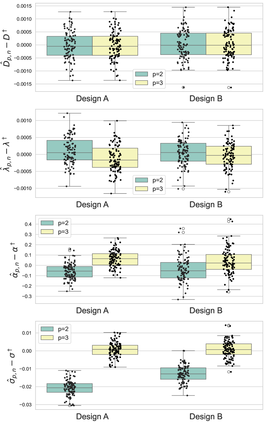
(a) Case I.

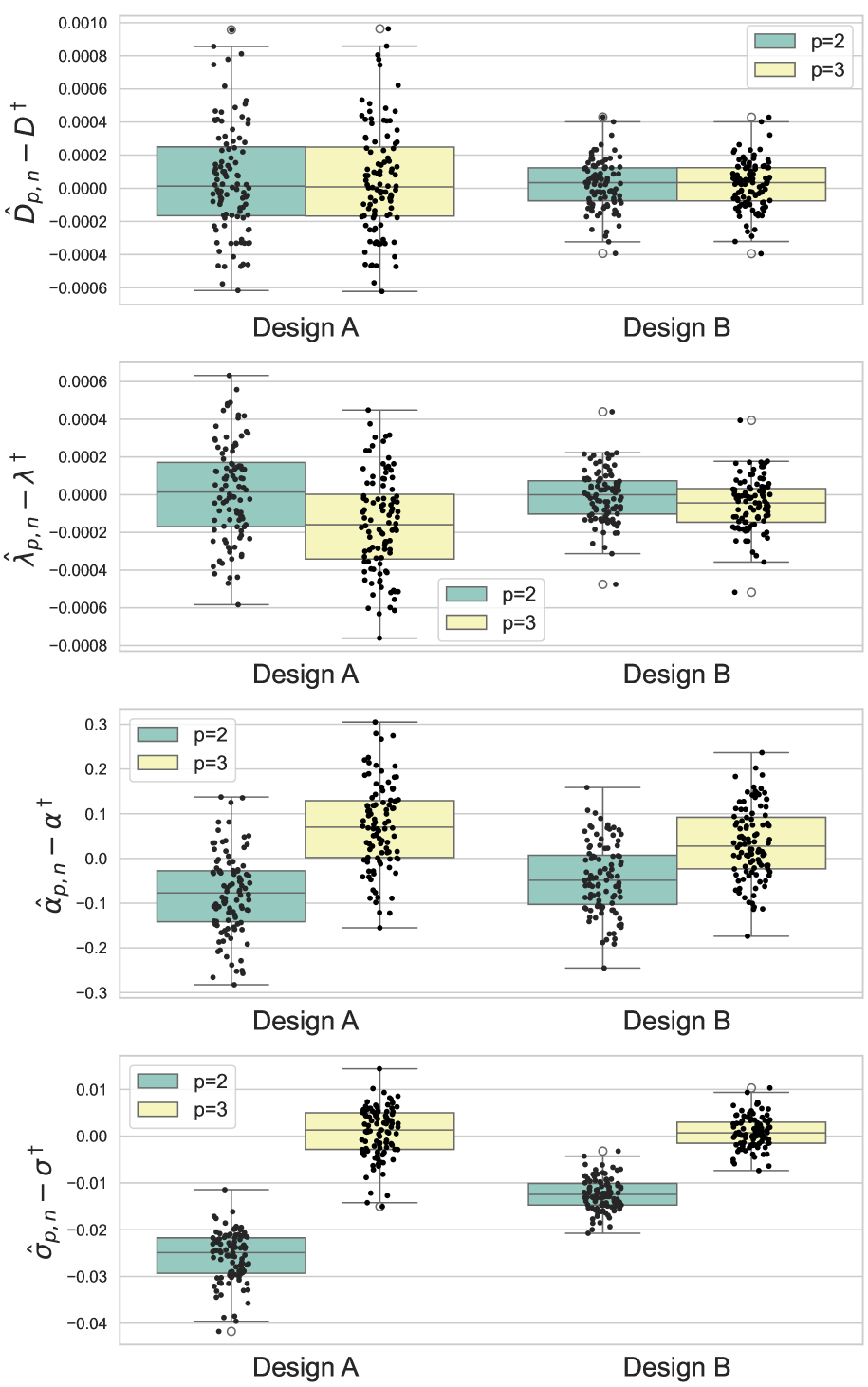
(b) Case II.

Figure 1: Boxplots of $\displaystyle M=100$ independent realisations of (maximum likelihood estimate) $\displaystyle-$ (true value) for the models Case I (left panel) and Case II (right panel). The black points indicate the individual realisations.

4.2 FitzHugh-Nagumo Model

We consider the FitzHugh-Nagumo (FHN) model belonging in class (Hypo-I), and specified via the following bivariate SDE:

$$\displaystyle\begin{aligned} dX_{t}&=\tfrac{1}{\varepsilon}(X_{t}-(X_{t})^{3}-Y_{t}-s)dt;\\ dY_{t}&=(\gamma X_{t}-Y_{t}+\alpha)dt+\sigma dW_{t}^{1},\end{aligned}$$ (4.1)

with $\displaystyle\theta=(\varepsilon,\gamma,\alpha,\sigma)$ being the parameter vector to be estimated. We consider parameter estimation of the FHN model in both complete and partial observation regimes where only the component $\displaystyle X_{t}$ is observed in the latter case.

4.2.1 Complete Observation Regime

We consider the estimator $\displaystyle\hat{\theta}_{p,n}(=\hat{\theta}_{p,n}^{\,(\mathrm{I})})=(\hat{\varepsilon}_{p,n},\hat{\gamma}_{p,n},\hat{\alpha}_{p,n},\hat{\sigma}_{p,n})$ when $\displaystyle p=2,4$. Following Melnykova (2020), we fix $\displaystyle s=0.01$ and set the true values to $\displaystyle\theta^{\dagger}=(0.10,1.50,0.30,0.60)$. We generate $\displaystyle M=50$ independent observation trajectories by using the local Gaussian discretisation for the (Hypo-I) class defined in (Gloter and Yoshida, 2020; Iguchi et al., 2022) with a step-size $\displaystyle\Delta=10^{-4}$. Then, we obtain $\displaystyle M=50$ synthetic datasets of complete observations for the FHN model by sub-sampling from the above trajectories so that the data design uses $\displaystyle n=250,000$, $\displaystyle T_{n}=5,000$ and $\displaystyle\Delta_{n}=0.02$. To obtain the minima of the contrast functions we used the Adam optimiser with the same setting as the experiments with the $\displaystyle q$-GLE earlier, except for (step-size) = 0.01. Table 5 summarises the mean and standard deviation from the $\displaystyle 50$ realisations of $\displaystyle\hat{\theta}_{p,n}-\theta^{\dagger}$ for $\displaystyle p=2,4$ and Figure 2 shows boxplots of the corresponding $\displaystyle 50$ realisations of relative discrepancies $\displaystyle(\hat{\theta}_{p,n}^{j}-\theta^{\dagger,j})/\theta^{\dagger,j}$, $\displaystyle 1\leq j\leq 4$. We observe that the means of $\displaystyle\hat{\theta}_{p,n}-\theta^{\dagger}$ with $\displaystyle p=4$ are closer to $\displaystyle 0$ than those with $\displaystyle p=2$ for all coordinates of $\displaystyle\theta$ while both estimators attain similar standard deviations. Importantly, when $\displaystyle p=2$, we see in Figure 2 that $\displaystyle\hat{\varepsilon}_{2,n}$ and $\displaystyle\hat{\sigma}_{2,n}$ are severely biased since the true values are not covered by the 50 realisations. In contrast, when $\displaystyle p=4$, the realisations of $\displaystyle\hat{\theta}_{4,n}$ are spread on areas close to the true parameter values.

Table 5: Mean and standard deviation (in parenthesis) of (contrast estimate) $\displaystyle-$ (true value) from $\displaystyle M=50$ sets of complete observations for the FHN model, under the design $\displaystyle n=250,000$, $\displaystyle T_{n}=5,000$, $\displaystyle\Delta_{n}=0.02$.

	$\displaystyle\hat{\varepsilon}_{p,n}-\varepsilon^{\dagger}$	$\displaystyle\hat{\gamma}_{p,n}-\gamma^{\dagger}$	$\displaystyle\hat{\alpha}_{p,n}-\alpha^{\dagger}$	$\displaystyle\hat{\sigma}_{p,n}-\sigma^{\dagger}$
$\displaystyle p=2$	$\displaystyle 0.00068\,(0.00002)$	$\displaystyle-0.01760\,(0.00858)$	$\displaystyle-0.00435\,(0.01045)$	$\displaystyle-0.01607\,(0.00067)$
$\displaystyle p=4$	$\displaystyle 0.00002\,(0.00002)$	$\displaystyle-0.00838\,(0.00860)$	$\displaystyle-0.00227\,(0.01051)$	$\displaystyle-0.00126\,(0.00068)$

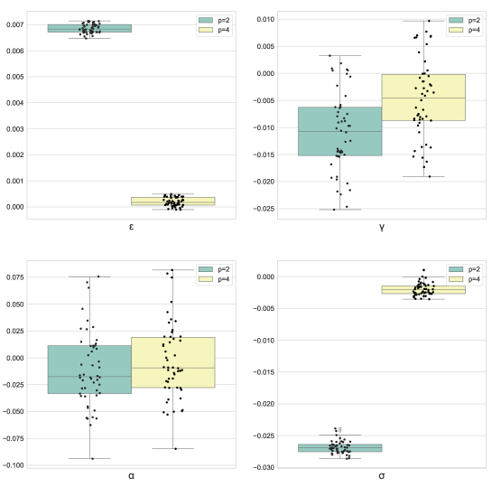
Figure 2: Boxplots of the $\displaystyle M=50$ realisations of $\displaystyle\bigl{(}\hat{\theta}_{p,n}-\theta^{\dagger}\bigr{)}/\theta^{\dagger}$ for the FHN model, under the design $\displaystyle n=250,000$, $\displaystyle T_{n}=5,000$, $\displaystyle\Delta_{n}=0.02$. The black points show the individual values.

4.2.2 Partial Observation Regime

We exploit the proposed contrast function, and the corresponding approximate log-likelihood, under the partial observation regime where only the smooth component $\displaystyle\{X_{t_{i}}\}$ is observed. In particular, we compute maximum likelihood estimators (MLEs) based upon a closed-form marginal likelihood constructed from the Gaussian approximation corresponding to the contrast function $\displaystyle\ell_{p,n}^{\,(\mathrm{I})}(\theta)$ for $\displaystyle p=2,3$. To be precise, we use the high-order expansions for the mean and the variance, but do not make use of the Taylor expansions for the inverse of the covariance and of its log-determinant, so that we obtain quantities that correspond to proper density functions. Here, we mention that due to the structure of the FHN model, the obtained one-step Gaussian approximation corresponding to the developed contrast function for $\displaystyle p=2,3$ is a linear Gaussian model w.r.t. the hidden component $\displaystyle Y_{t_{i}}$ given the observation $\displaystyle X_{t_{i}}$. Thus, one can make use of the Kalman Filter (KF) and calculate the marginal likelihood of the partial observations. For instance, see Iguchi et al. (2023) where a marginal likelihood is built upon KF for the $\displaystyle q$-GLE model belonging in the class (Hypo-II). We provide the details of the Gaussian approximation and the marginal likelihood for the FHN model in Appendix D. Then, the MLE for partial observation is defined as:

$$\displaystyle\hat{\theta}_{p,n}\bigl{(}=(\hat{\varepsilon}_{p,n},\hat{\gamma}_{p,n},\hat{\alpha}_{p,n},\hat{\sigma}_{p,n})\bigr{)}=\operatorname*{arg\,max}_{\theta\in\Theta}\log f_{p,n}(\{X_{t_{i}}\}_{i=0,\ldots,n};\theta),\quad p=2,3,$$ (4.2)

where $\displaystyle f_{p,n}(\{X_{t_{i}}\}_{i=0,\ldots,n};\theta)$, $\displaystyle p=2,3$, is the marginal likelihood. As with the experiment under complete observations, we fix $\displaystyle s=0.01$ and set the true values to $\displaystyle\theta^{\dagger}=(0.10,1.50,0.30,0.60)$. We generate $\displaystyle M=50$ independent observation trajectories from the LG discretisation with a step-size $\displaystyle\Delta=10^{-4}$. Then, we obtain $\displaystyle 50$ synthetic datasets of partial observation $\displaystyle\{X_{t_{i}}\}_{i=0,\ldots,n}$ with $\displaystyle n=200,000$, $\displaystyle T_{n}=1,000$ and $\displaystyle\Delta_{n}=0.005$ by sub-sampling from the above trajectories and removing the rough component $\displaystyle\{Y_{t_{i}}\}_{i=0,\ldots,n}$. The Nelder-Mead method is applied to optimise the log-marginal likelihood for $\displaystyle p=2,3$ with the initial guess $\displaystyle\theta_{0}=(0.5,0.5,0.5,0.5)$.

Table 6: Mean and standard deviation (in parenthesis) of $\displaystyle\hat{\theta}_{p,n}-\theta^{\dagger}$ from $\displaystyle M=50$ sets of partial observations for the FHN model, under the design $\displaystyle n=200,000$, $\displaystyle T_{n}=1,000$ and $\displaystyle\Delta_{n}=0.005$.

	$\displaystyle\hat{\varepsilon}_{p,n}-\varepsilon^{\dagger}$	$\displaystyle\hat{\gamma}_{p,n}-\gamma^{\dagger}$	$\displaystyle\hat{\alpha}_{p,n}-\alpha^{\dagger}$	$\displaystyle\hat{\sigma}_{p,n}-\sigma^{\dagger}$
$\displaystyle p=2$	$\displaystyle 0.00114\,(0.00049)$	$\displaystyle 0.01509\,(0.02432)$	$\displaystyle 0.00194\,(0.02063)$	$\displaystyle-0.00053\,(0.00294)$
$\displaystyle p=3$	$\displaystyle 0.00027\,(0.00048)$	$\displaystyle 0.00221\,(0.02425)$	$\displaystyle-0.00073\,(0.02044)$	$\displaystyle 0.00334\,(0.00286)$

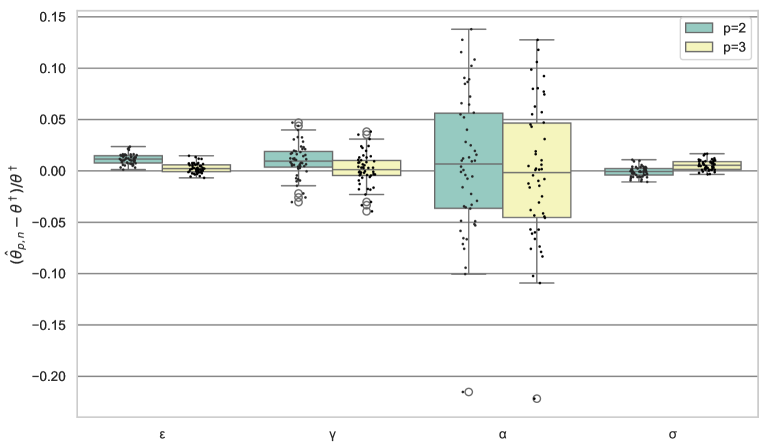
Figure 3: Boxplots of $\displaystyle\bigl{(}\hat{\theta}_{p,n}-\theta^{\dagger}\bigr{)}/\theta^{\dagger}$ from $\displaystyle M=50$ sets of partial observations for the FHN model, under the design $\displaystyle n=200,000$, $\displaystyle T_{n}=1,000$ and $\displaystyle\Delta_{n}=0.005$. The black points show the individual values.

Table 6 summarises the mean and standard deviation from the $\displaystyle 50$ realisations of $\displaystyle\hat{\theta}_{p,n}-\theta^{\dagger}$ for $\displaystyle p=2,3$ and Figure 3 shows boxplots of the corresponding $\displaystyle 50$ realisations of relative discrepancies $\displaystyle(\hat{\theta}_{p,n}^{j}-\theta^{\dagger,j})/\theta^{\dagger,j}$, $\displaystyle 1\leq j\leq 4$. First, we observe that both estimators share almost the same standard deviations. Secondly, the bias in $\displaystyle\hat{\varepsilon}_{2,n}$ is clear from the boxplot in the sense that the true value $\displaystyle\varepsilon^{\dagger}$ is not included in the interval between the minimum and the maximum of the $\displaystyle 50$ realisations of $\displaystyle\hat{\varepsilon}_{2,n}$. Finally, the square of the mean of $\displaystyle\hat{\theta}_{p,n}-\theta^{\dagger}$ (eq. bias) is reduced in the drift parameters ($\displaystyle\varepsilon$, $\displaystyle\gamma$ and $\displaystyle\alpha$) for $\displaystyle p=3$.

5 Proof of Main Results

We provide the proof for our main results, i.e. Theorems 3.1 and 3.2, which demonstrate the asymptotic normality of the proposed contrast estimators under the design condition $\displaystyle\Delta_{n}=o(n^{-1/p})$, $\displaystyle p\geq 2$. We show all details of the proof for the degenerate class (Hypo-II) as the proof for the class (Hypo-I) follows from similar arguments. Throughout this section, for simplicity of notation, we frequently omit the subscript $\displaystyle(\mathrm{II})$ appearing in the estimator and the functions introduced in Section 2.2.3. A number of technical results are collected in an Appendix. Throughout the proof, we make use of the notation $\displaystyle o_{\mathbb{P}_{\theta^{\dagger}}}(\cdot)$: for a sequence of random variables $\displaystyle\{F_{n}\}$ and a numerical sequence $\displaystyle\{\alpha_{n,\Delta_{n}}\}$ depending on $\displaystyle n$ or $\displaystyle\Delta_{n}$, we write $\displaystyle F_{n}=o_{\mathbb{P}_{\theta^{\dagger}}}(\alpha_{n,\Delta_{n}})$ if

$${F_{n}}/{\alpha_{n,\Delta_{n}}}\xrightarrow{\mathbb{P}_{\theta^{\dagger}}}0$$

as $\displaystyle n\to\infty$, $\displaystyle\Delta_{n}\to 0$ and $\displaystyle n\Delta_{n}\to\infty$.

5.1 Proof of Theorem 3.1 (Consistency)

We show the consistency of the contrast estimator via the following procedure:

Step 1.

We show that if $\displaystyle n\to\infty$, $\displaystyle\Delta_{n}\to 0$ and $\displaystyle n\Delta_{n}\to\infty$, then $\displaystyle\hat{\beta}_{S_{1},p,n}\xrightarrow{\mathbb{P}_{\theta^{\dagger}}}\beta_{S_{1}}^{\dagger}$. In particular,

$$\displaystyle\hat{\beta}_{S_{1},p,n}-\beta_{S_{1}}^{\dagger}=o_{\mathbb{P}_{\theta^{\dagger}}}(\sqrt{\Delta_{n}^{3}}).$$ (5.1)

Step 2.

Making use of the rate of convergence found in (5.1), we show that if $\displaystyle n\to\infty$, $\displaystyle\Delta_{n}\to 0$ and $\displaystyle n\Delta_{n}\to\infty$, then $\displaystyle\hat{\beta}_{S_{2},p,n}\xrightarrow{\mathbb{P}_{\theta^{\dagger}}}\beta_{S_{2}}^{\dagger}$. In particular,

$$\displaystyle\hat{\beta}_{S_{2},p,n}-\beta_{S_{2}}^{\dagger}=o_{\mathbb{P}_{\theta^{\dagger}}}(\sqrt{\Delta_{n}}).$$ (5.2)

Step 3.

Using the rates obtained in (5.1)-(5.2), we show that if $\displaystyle n\to\infty$, $\displaystyle\Delta_{n}\to 0$ and $\displaystyle n\Delta_{n}\to\infty$, then $\displaystyle(\hat{\beta}_{R,p,n},\hat{\sigma}_{p,n})\xrightarrow{\mathbb{P}_{\theta^{\dagger}}}(\beta^{\dagger}_{R},\sigma^{\dagger})$.

In the sequel, we express the matrix $\displaystyle\mathbf{\Lambda}(x,\theta)=(\mathbf{\Sigma}^{(\mathrm{II})}(x,\theta))^{-1},\,(x,\theta)\in\mathbb{R}^{N}\times\Theta$ as:

$$\displaystyle\mathbf{\Lambda}(x,\theta) \displaystyle=\begin{bmatrix}\mathbf{\Lambda}_{S_{1}S_{1}}(x,\theta)&\mathbf{\Lambda}_{S_{1}S_{2}}(x,\theta)&\mathbf{\Lambda}_{S_{1}R}(x,\theta)\\[5.69046pt] \mathbf{\Lambda}_{S_{2}S_{1}}(x,\theta)&\mathbf{\Lambda}_{S_{2}S_{2}}(x,\theta)&\mathbf{\Lambda}_{S_{2}R}(x,\theta)\\[5.69046pt] \mathbf{\Lambda}_{RS_{1}}(x,\theta)&\mathbf{\Lambda}_{RS_{2}}(x,\theta)&\mathbf{\Lambda}_{RR}(x,\theta)\end{bmatrix},$$

for block matrices $\displaystyle\mathbf{\Lambda}_{\iota_{1}\iota_{2}}(x,\theta)\in\mathbb{R}^{N_{\iota_{1}}\times N_{\iota_{2}}}$, $\displaystyle\iota_{1},\iota_{2}\in\{S_{1},S_{2},R\}$. In particular, from Lemma 13 in (Iguchi et al., 2023) we have:

$$\displaystyle\mathbf{\Lambda}_{S_{1}S_{1}}(x,\theta)=720\,a_{S_{1}}^{-1}(x,\theta),\qquad(x,\theta)\in\mathbb{R}^{N}\times\Theta,$$

where $\displaystyle a_{S_{1}}(x,\theta)$ is specified in the definition of the matrix $\displaystyle\mathbf{\Sigma}^{\,(\mathrm{II})}(x,\theta)$ in (2.7).

Remark 5.1.

The strategy of the proof outlined above is technically different from proofs in Melnykova (2020) and Gloter and Yoshida (2020), where they require the condition $\displaystyle\Delta_{n}=o(n^{-1/2})$ to prove consistency. Our proof of consistency proceeds without relying on the condition $\displaystyle\Delta_{n}=o(n^{-1/2})$, and such an approach then leads to a CLT under the weaker design condition $\displaystyle\Delta_{n}=o(n^{-1/p})$, $\displaystyle p\geq 2$. More details on this point can be found later in Remark 5.2.

5.1.1 Step 1.

The consistency of the estimator $\displaystyle\hat{\beta}_{S_{1},p,n}$ is deduced from the following result.

Lemma 5.1.

Assume $\displaystyle[\mathrm{H}1]$–$\displaystyle[\mathrm{H}5]$ hold. If $\displaystyle n\to\infty$, $\displaystyle\Delta_{n}\to 0$ and $\displaystyle n\Delta_{n}\to\infty$, then

$$\displaystyle\sup_{\theta\in\Theta}\,\Bigl{|}\tfrac{\Delta_{n}^{3}}{n}\ell_{p,n}(\theta)-\mathbf{Y}_{1}(\theta)\Bigr{|}\xrightarrow{\mathbb{P}_{\theta^{\dagger}}}0,$$ (5.3)

where

$$\displaystyle\mathbf{Y}_{1}(\theta)=\int\bigl{(}\mu_{S_{1}}(x_{S},\beta_{S_{1}})-\mu_{S_{1}}(x_{S},\beta^{\dagger}_{S_{1}})\bigr{)}^{\top}\mathbf{\Lambda}_{S_{1}S_{1}}(x,\theta)\bigl{(}\mu_{S_{1}}(x_{S},\beta_{S_{1}})-\mu_{S_{1}}(x_{S},\beta^{\dagger}_{S_{1}})\bigr{)}\nu_{\theta^{\dagger}}(dx),\quad\theta\in\Theta.$$

The proof is given in Appendix B.1. Lemma 5.1 indeed implies the consistency of $\displaystyle\hat{\beta}_{S_{1},p,n}$ via the following arguments. We first notice that the matrix $\displaystyle\mathbf{\Lambda}_{S_{1}S_{1}}(x,\theta)=720a_{S}^{-1}(x,\theta)$ is positive definite for any $\displaystyle(x,\theta)\in\mathbb{R}^{N}\times\Theta$ under $\displaystyle[\mathrm{H}1]$ due to Lemma 2.2. From the identifiability condition $\displaystyle[\mathrm{H}6]$ and the positive definiteness of $\displaystyle\mathbf{\Lambda}_{S_{1}S_{1}}$, the term $\displaystyle\mathbf{Y}_{1}(\theta)$, $\displaystyle\theta\in\Theta$, should be positive if $\displaystyle\beta_{S_{1}}\neq\beta^{\dagger}_{S_{1}}$. Thus, for any $\displaystyle\varepsilon>0$, there exists a constant $\displaystyle\delta>0$ so that

$$\displaystyle\mathbb{P}_{\theta^{\dagger}}\bigl{(}|\hat{\beta}_{S_{1},p,n}-\beta^{\dagger}_{S_{1}}|>\varepsilon\bigr{)} \displaystyle\leq\mathbb{P}_{\theta^{\dagger}}\Bigl{(}\mathbf{Y}_{1}(\hat{\theta}_{p,n})>\delta\Bigr{)}.$$

From the definition of the estimator and Lemma 5.1, we have:

$$\displaystyle\mathbb{P}_{\theta^{\dagger}}\Bigl{(}\mathbf{Y}_{1}(\hat{\theta}_{p,n})>\delta\Bigr{)} \displaystyle\leq\mathbb{P}_{\theta^{\dagger}}\Bigl{(}\tfrac{\Delta_{n}^{3}}{n}\ell_{p,n}(\beta^{\dagger}_{S_{1}},\hat{\beta}_{S_{2},p,n},\hat{\beta}_{R,p,n},\hat{\sigma}_{p,n})-\tfrac{\Delta_{n}^{3}}{n}\ell_{p,n}\bigl{(}\hat{\theta}_{p,n}\bigr{)}+\mathbf{Y}_{1}(\hat{\theta}_{p,n})>\delta\Bigr{)}$$

$$\displaystyle\leq\mathbb{P}_{\theta^{\dagger}}\Bigl{(}\,\sup_{\theta\in\Theta}\Bigl{|}\tfrac{\Delta_{n}^{3}}{n}\ell_{p,n}(\beta^{\dagger}_{S_{1}},{\beta}_{S_{2}},{\beta}_{R},{\sigma})-\tfrac{\Delta_{n}^{3}}{n}\ell_{p,n}\bigl{(}{\theta}\bigr{)}+\mathbf{Y}_{1}({\theta})\Bigr{|}>\delta\Bigr{)}\to 0,$$

as $\displaystyle n\to\infty$, $\displaystyle\Delta_{n}\to 0$ and $\displaystyle n\Delta_{n}\to\infty$, thus $\displaystyle\hat{\beta}_{S_{1},p,n}$ is a consistent estimator.

We now prove convergence (5.1). A Taylor expansion of $\displaystyle\partial_{\beta_{S_{1}}}\ell_{p,n}(\hat{\theta}_{p,n})$ at $\displaystyle(\beta^{\dagger}_{S_{1}},\hat{\beta}_{S_{2},p,n},\hat{\beta}_{R,p,n},\hat{\sigma}_{p,n})$ gives

$$\displaystyle\textbf{A}_{p,n}\bigl{(}\beta^{\dagger}_{S_{1}},\hat{\beta}_{S_{2},p,n},\hat{\beta}_{R,p,n},\hat{\sigma}_{p,n}\bigr{)}=\textbf{B}_{p,n}\bigl{(}\hat{\theta}_{p,n}\bigr{)}\;\times\tfrac{1}{\sqrt{\Delta_{n}^{3}}}(\hat{\beta}_{S_{1},p,n}-\beta^{\dagger}_{S_{1}}),$$

where we have set, for $\displaystyle\theta=(\beta_{S_{1}},\theta^{S_{2},R})\in\Theta$, $\displaystyle\theta^{S_{2},R}\equiv(\beta_{S_{2}},\beta_{R},\sigma)\in\Theta_{\beta_{S_{2}}}\times\Theta_{\beta_{R}}\times\Theta_{\sigma}$,

$$\displaystyle\mathbf{A}_{p,n}\bigl{(}\theta\bigr{)}=-\tfrac{\sqrt{\Delta_{n}^{3}}}{n}\partial_{\beta_{S_{1}}}\ell_{p,n}\bigl{(}\theta\bigr{)},\quad\textbf{B}_{p,n}\bigl{(}\theta\bigr{)}=\tfrac{\Delta_{n}^{3}}{n}\int_{0}^{1}\partial_{\beta_{S_{1}}}^{2}\ell_{p,n}\bigl{(}\beta^{\dagger}_{S_{1}}+\lambda({\beta}_{S_{1}}-\beta^{\dagger}_{S_{1}}),\theta^{S_{2},R}\bigr{)}d\lambda.$$

The convergence (5.1) holds from the following result whose proof is given in Appendix B.2.

Lemma 5.2.

Assume $\displaystyle[\mathrm{H}1]$–$\displaystyle[\mathrm{H}6]$. If $\displaystyle n\to\infty$, $\displaystyle\Delta_{n}\to 0$ and $\displaystyle n\Delta_{n}\to\infty$, then

$$\displaystyle\sup_{(\beta_{S_{2}},\beta_{R},\sigma)\in\Theta_{\beta_{S_{2}}}\times\Theta_{\beta_{R}}\times\Theta_{\sigma}}\Bigl{|}\mathbf{A}_{p,n}\bigl{(}\beta^{\dagger}_{S_{1}},\beta_{S_{2}},\beta_{R},\sigma\bigr{)}\Bigr{|}\xrightarrow{\mathbb{P}_{\theta^{\dagger}}}0;$$ (5.4)

$$\displaystyle\sup_{(\beta_{S_{2}},\beta_{R},\sigma)\in\Theta_{\beta_{S_{2}}}\times\Theta_{\beta_{R}}\times\Theta_{\sigma}}\Bigl{|}\mathbf{B}_{p,n}\bigl{(}\hat{\beta}_{S_{1},p,n},\beta_{S_{2}},\beta_{R},\sigma\bigr{)}-2\mathbf{{B}}\bigl{(}\beta^{\dagger}_{S_{1}},\beta_{S_{2}},\sigma\bigr{)}\Bigr{|}\xrightarrow{\mathbb{P}_{\theta^{\dagger}}}0,$$ (5.5)

where for $\displaystyle(\beta_{S_{2}},\beta_{R},\sigma)\in\Theta_{\beta_{S_{2}}}\times\Theta_{\beta_{R}}\times\Theta_{\sigma}$,

$$\displaystyle\mathbf{{B}}\bigl{(}{\beta}_{S_{1}},\beta_{S_{2}},\sigma\bigr{)}=720\int\bigl{(}\partial_{\beta_{S_{1}}}^{\top}\mu_{S_{1}}(x_{S},\beta_{S_{1}})\bigr{)}^{\top}a_{S_{1}}^{-1}(x,(\beta_{S_{1}},\beta_{S_{2}},\sigma))\partial_{\beta_{S_{1}}}^{\top}\mu_{S_{1}}(x_{S},\beta_{S_{1}})\,\nu_{\theta^{\dagger}}(dx).$$

Remark 5.2.

We point here to a key fact to obtain (5.4) leading to the rate $\displaystyle\hat{\beta}_{S_{1},p,n}-\beta^{\dagger}_{S_{1}}=o_{\mathbb{P}_{\theta^{\dagger}}}(\sqrt{\Delta_{n}^{3}})$. The term $\displaystyle\mathbf{A}_{p,n}$ is given in the form of

$$\displaystyle\mathbf{A}_{p,n}(\beta^{\dagger}_{S_{1}},\beta_{S_{2}},\beta_{R},\sigma)=\tfrac{1}{n\sqrt{\Delta_{n}}}\sum_{i=1}^{n}F(1,{X}_{t_{i-1}},(\beta^{\dagger}_{S_{1}},\beta_{S_{2}},\beta_{R},\sigma))+R(\Delta_{n},(\beta^{\dagger}_{S_{1}},\beta_{S_{2}},\beta_{R},\sigma)),$$ (5.6)

where $\displaystyle F=[F^{k}]_{1\leq k\leq N_{\beta_{S_{1}}}}$ with $\displaystyle F^{k}\in\mathcal{S}$, and the second term is a residual such that

$$\sup_{(\beta_{S_{2}},\beta_{R},\sigma)\in\Theta_{\beta_{S_{2}}}\times\Theta_{\beta_{R}}\times\Theta_{\sigma}}\bigl{|}R(\Delta_{n},(\beta^{\dagger}_{S_{1}},\beta_{S_{2}},\beta_{R},\sigma))\bigr{|}\xrightarrow{\mathbb{P}_{\theta^{\dagger}}}0.$$

The first term of the right hand side of (5.6) includes $\displaystyle\Delta_{n}^{-1/2}$, however $\displaystyle F^{k}(1,x,\theta)$ is identically $\displaystyle 0$ for any $\displaystyle(x,\theta)\in\mathbb{R}^{N}\times\Theta$ following some matrix algebra (as indicated in Lemma B.1 in the Appendix) and then (5.4) holds. A similar argument related with matrix algebra (see, e.g., Lemmas B.2, B.3) is also used in the proofs of other technical lemmas below to deal with terms of size $\displaystyle\mathcal{O}(\Delta_{n}^{-1/2})$, and then the proof of consistency proceeds without requiring that $\displaystyle\Delta_{n}=o(n^{-1/2})$.

5.1.2 Step 2

Making use of convergence (5.1), we obtain the following result whose proof is postponed to Appendix B.3.

Lemma 5.3.

Assume $\displaystyle[\mathrm{H}1]$–$\displaystyle[\mathrm{H}6]$ hold. If $\displaystyle n\to\infty$, $\displaystyle\Delta_{n}\to 0$ and $\displaystyle n\Delta_{n}\to\infty$, then

$$\displaystyle\sup_{(\beta_{S_{2}},\beta_{R},\sigma)\in\Theta_{\beta_{S_{2}}}\times\Theta_{\beta_{R}}\times\Theta_{\sigma}}\Bigl{|}\tfrac{\Delta_{n}}{n}\ell_{p,n}(\hat{\beta}_{S_{1},p,n},\beta_{S_{2}},\beta_{R},\sigma)-\mathbf{Y}_{2}(\beta_{S_{2}},\beta_{R},\sigma)\Bigr{|}\xrightarrow{\mathbb{P}_{\theta^{\dagger}}}0,$$

where

$$\displaystyle\mathbf{Y}_{2}(\beta_{S_{2}},\beta_{R},\sigma)=12\int\bigl{(}\mu_{S_{2}}(x,\beta_{S_{2}})-\mu_{S_{2}}(x,\beta^{\dagger}_{S_{2}})\bigr{)}^{\top}a_{S_{2}}^{-1}\bigl{(}x,(\beta^{\dagger}_{S_{1}},\beta_{S_{2}},\sigma)\bigr{)}\bigl{(}\mu_{S_{2}}(x,\beta_{S_{2}})-\mu_{S_{2}}(x,\beta^{\dagger}_{S_{2}})\bigr{)}\nu_{\theta^{\dagger}}(dx).$$

Lemma 5.3 leads to the consistency of $\displaystyle\hat{\beta}_{S_{2},p,n}$ following arguments similar to the ones used in Section 5.1.1 to show the consistency of $\displaystyle\hat{\beta}_{S_{1},p,n}$.

To obtain the rate of convergence in (5.2), we consider the Taylor expansion of $\displaystyle\partial_{\beta_{S}}\ell_{p,n}(\hat{\theta}_{p,n})$ at $\displaystyle(\beta^{\dagger}_{S},\hat{\beta}_{R,p,n},\hat{\sigma}_{p,n})$:

$$\displaystyle\widetilde{\mathbf{A}}_{p,n}\bigl{(}\beta^{\dagger}_{S_{1}},\beta^{\dagger}_{S_{2}},\hat{\beta}_{R,p,n},\hat{\sigma}_{p,n}\bigr{)}=\widetilde{\mathbf{B}}_{p,n}\bigl{(}\hat{\theta}_{p,n}\bigr{)}\begin{bmatrix}\tfrac{1}{\sqrt{\Delta_{n}^{3}}}(\hat{\beta}_{S_{1},p,n}-\beta^{\dagger}_{S_{1}})\\[5.69046pt] \tfrac{1}{\sqrt{\Delta_{n}}}(\hat{\beta}_{S_{2},p,n}-\beta^{\dagger}_{S_{2}})\end{bmatrix},$$ (5.7)

where we have set for $\displaystyle\theta=(\beta_{S},\beta_{R},\sigma)\in\Theta$ with $\displaystyle\beta_{S}=(\beta_{S_{1}},\beta_{S_{2}})\in\Theta_{\beta_{S}}$,

$$\displaystyle\widetilde{\mathbf{A}}_{p,n}\bigl{(}\theta\bigr{)}=\begin{bmatrix}-\tfrac{\sqrt{\Delta_{n}^{3}}}{n}\partial_{\beta_{S_{1}}}\ell_{p,n}(\theta)\\[5.69046pt] -\tfrac{\sqrt{\Delta_{n}}}{n}\partial_{\beta_{S_{2}}}\ell_{p,n}(\theta)\end{bmatrix},\qquad\widetilde{\mathbf{B}}_{p,n}\bigl{(}\theta\bigr{)}=\widetilde{\mathbf{M}}_{n}\Bigl{(}\int_{0}^{1}\,\partial_{\beta_{S}}^{2}\ell_{p,n}\bigl{(}\beta^{\dagger}_{S}+\lambda(\beta_{S}-\beta^{\dagger}_{S}),\beta_{R},\sigma\bigr{)}d\lambda\,\Bigr{)}\widetilde{\mathbf{M}}_{n}^{\top},$$

for the matrix $\displaystyle\widetilde{\mathbf{M}}_{n}=\mathrm{Diag}(v_{n})$, where

$$\displaystyle v_{n}=\Bigl{[}\underbrace{\sqrt{\tfrac{\Delta_{n}^{3}}{n}},\ldots,\sqrt{\tfrac{\Delta_{n}^{3}}{n}}}_{N_{\beta_{S_{1}}}},\;\underbrace{\sqrt{\tfrac{\Delta_{n}}{n}},\ldots,\sqrt{\tfrac{\Delta_{n}}{n}}}_{N_{\beta_{S_{2}}}}\Bigr{]}^{\top}.$$

The convergence (5.2) is immediately deduced from equation (5.7) given the following result whose proof is provided in Appendix B.4.

Lemma 5.4.

Assume that $\displaystyle[\mathrm{H}1]$–$\displaystyle[\mathrm{H}6]$ hold. If $\displaystyle n\to\infty$, $\displaystyle\Delta_{n}\to 0$ and $\displaystyle n\Delta_{n}\to\infty$, then

$$\displaystyle\sup_{(\beta_{R},\sigma)\in\Theta_{\beta_{R}}\times\Theta_{\sigma}}\Bigl{|}\widetilde{\mathbf{A}}_{p,n}\bigl{(}\beta^{\dagger}_{S},\beta_{R},\sigma\bigr{)}\Bigr{|}\xrightarrow{\mathbb{P}_{\theta^{\dagger}}}0;$$ (5.8)

$$\displaystyle\sup_{(\beta_{R},\sigma)\in\Theta_{\beta_{R}}\times\Theta_{\sigma}}\Bigl{|}\widetilde{\mathbf{B}}_{p,n}\bigl{(}\beta^{\dagger}_{S},\beta_{R},\sigma\bigr{)}-2\,\widetilde{\mathbf{B}}\bigl{(}\beta^{\dagger}_{S},\beta_{R},\sigma\bigr{)}\Bigr{|}\xrightarrow{\mathbb{P}_{\theta^{\dagger}}}0;,$$ (5.9)

where we have set for $\displaystyle\theta\in\Theta$,

$$\displaystyle\widetilde{\mathbf{B}}\bigl{(}\theta\bigr{)}=\mathrm{Diag}\Bigl{[}\widetilde{\mathbf{B}}^{S_{1}}(\theta),\;\widetilde{\mathbf{B}}^{S_{2}}(\theta)\Bigr{]}$$

with $\displaystyle\widetilde{\mathbf{B}}^{S_{1}}(\theta)\in\mathbb{R}^{N_{\beta_{S_{1}}}\times N_{\beta_{S_{1}}}}$ and $\displaystyle\widetilde{\mathbf{B}}^{S_{2}}(\theta)\in\mathbb{R}^{N_{\beta_{S_{2}}}\times N_{\beta_{S_{2}}}}$ defined as:

$$\displaystyle\widetilde{\mathbf{B}}^{S_{1}}(\theta) \displaystyle=720\int\bigl{(}\partial_{\beta_{S_{1}}}^{\top}\mu_{S_{1}}(x_{S},\beta_{S_{1}})\bigr{)}^{\top}a_{S_{1}}^{-1}(x,\theta)\,\partial_{\beta_{S_{1}}}^{\top}\mu_{S_{1}}(x_{S},\beta_{S_{1}})\nu_{\theta^{\dagger}}(dx);$$ (5.10)

$$\displaystyle\widetilde{\mathbf{B}}^{S_{2}}(\theta) \displaystyle=12\int\bigl{(}\partial_{\beta_{S_{2}}}^{\top}\mu_{S_{2}}(x,\beta_{S_{2}})\bigr{)}^{\top}a_{S_{2}}^{-1}(x,\theta)\,\partial_{\beta_{S_{2}}}^{\top}\mu_{S_{2}}(x,\beta_{S_{2}})\nu_{\theta^{\dagger}}(dx).$$ (5.11)

5.1.3 Step 3

Finally, we show the consistency of estimators $\displaystyle\bigl{(}\hat{\beta}_{R,p,n},\hat{\sigma}_{p,n}\bigr{)}$. Working with the rates of convergence obtained in (5.1) and (5.2), we prove the following result leading to the consistency of $\displaystyle\hat{\sigma}_{p,n}$.

Lemma 5.5.

Assume $\displaystyle[\mathrm{H}1]$–$\displaystyle[\mathrm{H}6]$ hold. If $\displaystyle n\to\infty$, $\displaystyle\Delta_{n}\to 0$ and $\displaystyle n\Delta_{n}\to\infty$, then

$$\displaystyle\sup_{(\beta_{R},\sigma)\in\Theta_{\beta_{R}}\times\Theta_{\sigma}}\Bigl{|}\tfrac{1}{n}\ell_{p,n}\bigl{(}\hat{\beta}_{S,p,n},\beta_{R},\sigma\bigr{)}-\mathbf{Y}_{3}(\sigma)\Bigr{|}\xrightarrow{\mathbb{P}_{\theta^{\dagger}}}0,$$

where we have set for $\displaystyle\sigma\in\Theta_{\sigma}$,

$$\displaystyle\mathbf{Y}_{3}(\sigma)=\int\Bigl{\{}\mathrm{Tr}\bigl{(}\mathbf{\Lambda}(x,(\beta^{\dagger}_{S},\sigma))\mathbf{\Sigma}\bigl{(}x,(\beta^{\dagger}_{S},\sigma^{\dagger})\bigr{)}\bigr{)}+\log\det\mathbf{\Sigma}\bigl{(}x,(\beta^{\dagger}_{S},\sigma)\bigr{)}\Bigr{\}}\nu_{\theta^{\dagger}}(dx).$$

We provide the proof in Appendix B.5. We will show that Lemma 5.5 indeed leads to the consistency of $\displaystyle\hat{\sigma}_{p,n}$. We have

$$\displaystyle\mathbf{Y}_{3}(\sigma)-\mathbf{Y}_{3}(\sigma^{\dagger})=\int\Phi(x,\sigma)\,\nu_{\theta^{\dagger}}(dx),\quad\sigma\in\Theta,$$

where

$$\displaystyle\Phi(x,\sigma) \displaystyle=\mathrm{Tr}\bigl{(}\mathbf{\Lambda}(x,(\beta^{\dagger}_{S},\sigma))\mathbf{\Sigma}\bigl{(}x,(\beta^{\dagger}_{S},\sigma^{\dagger})\bigr{)}\bigr{)}-N-\log\tfrac{\det\mathbf{\Sigma}(x,(\beta^{\dagger}_{S},\sigma^{\dagger}))}{\det\mathbf{\Sigma}(x,(\beta^{\dagger}_{S},\sigma))}$$

$$\displaystyle=2\times\int\varphi(y;x,\sigma^{\dagger})\log\frac{\varphi(y;x,\sigma)}{\varphi(y;x,\sigma^{\dagger})}dy,$$

with $\displaystyle y\mapsto\varphi(y;x,\sigma),\,(x,\sigma)\in\mathbf{R}^{N}\times\Theta$ being the density of the distribution $\displaystyle\mathscr{N}(\mathbf{0}_{N},\mathbf{\Sigma}(x,(\beta^{\dagger}_{S},\sigma))$. Thus, under condition $\displaystyle[\mathrm{H}6]$, $\displaystyle\mathbf{Y}_{3}(\sigma)-\mathbf{Y}_{3}(\sigma^{\dagger})$ should be positive if $\displaystyle\sigma\neq\sigma^{\dagger}$. Hence, for every $\displaystyle\varepsilon>0$, there exists a constant $\displaystyle\delta>0$ so that

$$\displaystyle\mathbb{P}_{\theta^{\dagger}}\bigl{(}|\hat{\sigma}_{p,n}-\sigma^{\dagger}|>\varepsilon\bigr{)}\leq\mathbb{P}_{\theta^{\dagger}}\bigl{(}\mathbf{Y}_{3}(\hat{\sigma}_{p,n})-\mathbf{Y}_{3}(\sigma^{\dagger})>\delta\bigr{)}$$

$$\displaystyle\quad\leq\mathbb{P}_{\theta^{\dagger}}\Bigl{(}\tfrac{1}{n}\ell_{p,n}(\hat{\beta}_{p,n},\sigma^{\dagger})-\tfrac{1}{n}\ell_{p,n}(\hat{\theta}_{p,n})+\mathbf{Y}_{3}(\hat{\sigma}_{p,n})-\mathbf{Y}_{3}(\sigma^{\dagger})>\delta\Bigr{)}$$

$$\displaystyle\quad\leq\mathbb{P}_{\theta^{\dagger}}\Bigl{(}\sup_{(\beta_{R},\sigma)\in\Theta_{\beta_{R}}\times\Theta_{\sigma}}\Bigl{|}\tfrac{1}{n}\ell_{p,n}(\hat{\beta}_{S,p,n},\beta_{R},\sigma^{\dagger})-\tfrac{1}{n}\ell_{p,n}(\hat{\beta}_{S,p,n},\beta_{R},\sigma)+\mathbf{Y}_{3}(\sigma)-\mathbf{Y}_{3}(\sigma^{\dagger})\Bigr{|}>\delta\Bigr{)}\to 0,$$

as $\displaystyle n\to\infty$, $\displaystyle\Delta_{n}\to 0$ and $\displaystyle n\Delta_{n}\to\infty$.

To show the consistency of $\displaystyle\hat{\beta}_{R,p,n}$, we consider:

$$\displaystyle\mathbf{K}(\theta):=\tfrac{1}{n\Delta_{n}}\ell_{p,n}\bigl{(}\theta\bigr{)}-\tfrac{1}{n\Delta_{n}}\ell_{p,n}\bigl{(}\beta_{S_{1}},\beta_{S_{2}},\beta^{\dagger}_{R},\sigma\bigr{)},\quad\theta=(\beta_{S_{1}},\beta_{S_{2}},\beta_{R},\sigma)\in\Theta.$$ (5.12)

The consistency of the estimator $\displaystyle\hat{\beta}_{R,p,n}$ follows from the following result whose proof is given in Appendix B.6.

Lemma 5.6.

Assume $\displaystyle[\mathrm{H}1]$–$\displaystyle[\mathrm{H}6]$ hold. If $\displaystyle n\to\infty$, $\displaystyle\Delta_{n}\to 0$ and $\displaystyle n\Delta_{n}\to\infty$, then

$$\displaystyle\sup_{\beta_{R}\in\Theta_{\beta_{R}}}\Bigl{|}\mathbf{K}(\hat{\beta}_{S_{1},p,n},\hat{\beta}_{S_{2},p,n},\beta_{R},\hat{\sigma}_{p,n})-\mathbf{Y}_{4}(\beta_{R})\Bigr{|}\xrightarrow{\mathbb{P}_{\theta^{\dagger}}}0,$$

where we have set for $\displaystyle\beta_{R}\in\Theta_{\beta_{R}}$,

$$\displaystyle\mathbf{Y}_{4}(\beta_{R})=\int\bigl{(}\mu_{R}(x,\beta_{R})-\mu_{R}(x,\beta^{\dagger}_{R})\bigr{)}^{\top}a^{-1}_{R}(x,\sigma^{\dagger})\bigl{(}\mu_{R}(x,\beta_{R})-\mu_{R}(x,\beta^{\dagger}_{R})\bigr{)}\nu_{\theta^{\dagger}}(dx).$$

Thus, the proof of consistency for the proposed estimator is now complete.

5.2 Proof of Theorem 3.2 (CLT)

We define the $\displaystyle N_{\theta}\times N_{\theta}$ matrix $\displaystyle\mathbf{M}_{n}$ as:

$$\displaystyle\mathbf{M}_{n}=\mathrm{Diag}\Bigl{[}\underbrace{\sqrt{\tfrac{n}{\Delta_{n}^{3}}},\ldots,\sqrt{\tfrac{n}{\Delta_{n}^{3}}}}_{N_{\beta_{S_{1}}}},\;\underbrace{\sqrt{\tfrac{n}{\Delta_{n}}},\ldots,\sqrt{\tfrac{n}{\Delta_{n}}}}_{N_{\beta_{S_{2}}}},\;\underbrace{{\sqrt{n\Delta_{n}}},\ldots,{\sqrt{n\Delta_{n}}}}_{N_{\beta_{R}}},\;\underbrace{{\sqrt{n}},\ldots,{\sqrt{n}}}_{N_{\sigma}}\Bigr{]}.$$

Noting that $\displaystyle\partial_{\theta}\ell_{p,n}(\hat{\theta}_{p,n})=\mathbf{0}_{N_{\theta}}$, a Taylor expansion of $\displaystyle\partial_{\theta}\ell_{p,n}(\hat{\theta}_{p,n})$ at the true parameter $\displaystyle\theta^{\dagger}$ gives:

$$\displaystyle\mathbf{I}_{p,n}(\theta^{\dagger})=\int_{0}^{1}\mathbf{J}_{p,n}\bigl{(}\theta^{\dagger}+\lambda(\hat{\theta}_{p,n}-\theta^{\dagger})\bigr{)}d\lambda\times\begin{bmatrix}\sqrt{\tfrac{n}{\Delta^{3}_{n}}}\bigl{(}\hat{\beta}_{S_{1},p,n}-\beta^{\dagger}_{S_{1}}\bigr{)}\\[5.69046pt] \sqrt{\tfrac{n}{\Delta_{n}}}\bigl{(}\hat{\beta}_{S_{2},p,n}-\beta^{\dagger}_{S_{2}}\bigr{)}\\[5.69046pt] \sqrt{n\Delta_{n}}\bigl{(}\hat{\beta}_{R,p,n}-\beta^{\dagger}_{R}\bigr{)}\\[5.69046pt] \sqrt{n}\bigl{(}\hat{\sigma}_{p,n}-\sigma^{\dagger}\bigr{)}\end{bmatrix},$$ (5.13)

where we have set for $\displaystyle\theta\in\Theta$,

$$\displaystyle\mathbf{I}_{p,n}(\theta)\equiv-\mathbf{M}_{n}^{-1}\,\partial_{\theta}\ell_{p,n}(\theta),\qquad\mathbf{J}_{p,n}(\theta)\equiv\mathbf{M}_{n}^{-1}\,\partial^{2}_{\theta}\ell_{p,n}(\theta)\,\mathbf{M}_{n}^{-1}.$$

To prove the asymptotic normality, we obtain the following two results.

Lemma 5.7.

Let $\displaystyle p\geq 2$ be an integer. Assume that $\displaystyle[\mathrm{H}1]$–$\displaystyle[\mathrm{H}6]$ hold. If $\displaystyle n\to\infty$, $\displaystyle\Delta_{n}\to 0$ and $\displaystyle n\Delta_{n}\to\infty$, then

$$\displaystyle\sup_{\lambda\in[0,1]}\Bigl{|}\mathbf{J}_{p,n}\bigl{(}\theta^{\dagger}+\lambda(\hat{\theta}_{p,n}-\theta^{\dagger})\bigr{)}-2\Gamma(\theta^{\dagger})\Bigr{|}\xrightarrow{\mathbb{P}_{\theta^{\dagger}}}0.$$

Proposition 5.1.

Assume that $\displaystyle[\mathrm{H}1]$–$\displaystyle[\mathrm{H}5]$ hold. If $\displaystyle n\to\infty$, $\displaystyle\Delta_{n}\to 0$ and $\displaystyle n\Delta_{n}\to\infty$, with the additional design condition $\displaystyle\Delta_{n}=o(n^{-1/p})$, then

$$\displaystyle\mathbf{I}_{p,n}(\theta^{\dagger})\xrightarrow{\mathcal{L}_{\theta^{\dagger}}}\mathscr{N}\bigl{(}\mathbf{0}_{N_{\theta}},4\Gamma(\theta^{\dagger})\bigr{)}.$$

We provide the proof of Lemma 5.7 in Appendix C.1. We show the proof of Proposition 5.1 in the next subsection where we highlight the manner in which we make use of the condition $\displaystyle\Delta_{n}=o(n^{-1/p})$, $\displaystyle p\geq 2$. By applying these two results to equation (5.13), the proof of Theorem 3.2 is complete.

5.2.1 Proof of Proposition 5.1

For simplicity of notation, we write $\displaystyle\textstyle\partial_{\theta,k}\ell_{p,n}(\theta)=\sum_{i=1}^{n}{\xi}_{i}^{k}(\theta),\;\theta\in\Theta,\,1\leq k\leq N_{\theta}$, where

$$\displaystyle\xi_{i}^{k}(\theta)=[\mathbf{M}_{n}^{-1}]_{kk}\sum_{j=0}^{K_{p}}\,\Delta_{n}^{j}\times\partial_{\theta,k}\bigl{\{}\mathbf{m}_{p,i}(\Delta_{n},\theta)^{\top}\,\mathbf{G}_{i-1,j}(\theta)\,\mathbf{m}_{p,i}(\Delta_{n},\theta)+\mathbf{H}_{i-1,j}(\theta)\bigr{\}},\quad 1\leq i\leq n.$$ (5.14)

Due to Theorems 4.2 & 4.4 in Hall and Heyde (1980), Proposition 5.1 holds once we prove the following convergences:

(i)

If $\displaystyle n\to\infty$, $\displaystyle\Delta_{n}\to 0$ and $\displaystyle n\Delta_{n}\to\infty$  with $\displaystyle\Delta_{n}=o(n^{-1/p})$, then

$$\displaystyle\sum_{i=1}^{n}\mathbb{E}_{\theta^{\dagger}}\bigl{[}\xi_{i}^{k}(\theta^{\dagger})|\mathcal{F}_{t_{i-1}}\bigr{]}\xrightarrow{\mathbb{P}_{\theta^{\dagger}}}0,\quad 1\leq k\leq N_{\theta}.$$ (5.15)

(ii)

If $\displaystyle n\to\infty$, $\displaystyle\Delta_{n}\to 0$ and $\displaystyle n\Delta_{n}\to\infty$, then

$$\displaystyle\sum_{i=1}^{n}\mathbb{E}_{\theta^{\dagger}}\bigl{[}\xi_{i}^{k_{1}}(\theta^{\dagger})\xi_{i}^{k_{2}}(\theta^{\dagger})|\mathcal{F}_{t_{i-1}}\bigr{]}\xrightarrow{\mathbb{P}_{\theta^{\dagger}}}4\bigl{[}\Gamma(\theta^{\dagger})\bigr{]}_{k_{1}k_{2}},\quad 1\leq k_{1},k_{2}\leq N_{\theta};$$ (5.16)

$$\displaystyle\sum_{i=1}^{n}\mathbb{E}_{\theta^{\dagger}}\bigl{[}\bigl{(}\xi_{i}^{k_{1}}(\theta^{\dagger})\xi_{i}^{k_{2}}(\theta^{\dagger})\bigr{)}^{2}|\mathcal{F}_{t_{i-1}}\bigr{]}\xrightarrow{\mathbb{P}_{\theta^{\dagger}}}0,\quad 1\leq k_{1},k_{2}\leq N_{\theta}.$$ (5.17)

Notice that the design condition $\displaystyle\Delta_{n}=o(n^{-1/p})$ is used in the proof that the expectation of the score function converges to $\displaystyle 0$, i.e., for convergence (5.15). We provide the proof of the two convergences (5.16) and (5.17) in Appendix C.2 and focus on the proof of (5.15) in this section.

Proof of convergence (5.15). Let $\displaystyle 1\leq k\leq N_{\theta}$. We write for $\displaystyle\theta\in\Theta$ and $\displaystyle 1\leq i\leq n$,

$$\displaystyle\partial_{\theta,k}\mathbf{m}_{p,i}(\Delta_{n},\theta)\equiv v_{p,k}(\Delta_{n},{X}_{t_{i-1}},\theta).$$

Note that the $\displaystyle\mathbb{R}^{N}$-valued function $\displaystyle v_{p,k}(\Delta_{n},{X}_{t_{i-1}},\theta)$ is independent of $\displaystyle{X}_{t_{i}}$. It then follows that

$$\displaystyle\sum_{i=1}^{n}\mathbb{E}_{\theta^{\dagger}}\bigl{[}\xi_{i}^{k}(\theta^{\dagger})|\mathcal{F}_{t_{i-1}}\bigr{]}=\sum_{i=1}^{n}\bigl{\{}F^{(1),k}_{i-1}(\theta^{\dagger})+F^{(2),k}_{i-1}(\theta^{\dagger})\bigr{\}},$$

where we have set:

$$\displaystyle F^{(1),k}_{i-1}(\theta^{\dagger}) \displaystyle=2[\mathbf{M}_{n}^{-1}]_{kk}\sum_{j=0}^{K_{p}}\sum_{l_{1},l_{2}=1}^{N}\Delta_{n}^{j}\,v_{p,k}^{l_{1}}(\Delta_{n},{X}_{t_{i-1}},\theta^{\dagger})\bigl{[}\mathbf{G}_{i-1,j}(\theta^{\dagger})\bigr{]}_{l_{1}l_{2}}\mathbb{E}_{\theta^{\dagger}}\bigl{[}\mathbf{m}_{p,i}^{l_{2}}(\Delta_{n},\theta^{\dagger})|\mathcal{F}_{t_{i-1}}\bigr{]};$$

$$\displaystyle F^{(2),k}_{i-1}(\theta^{\dagger}) \displaystyle=[\mathbf{M}_{n}^{-1}]_{kk}\sum_{j=0}^{K_{p}}\Delta_{n}^{j}\Bigl{\{}\sum_{l_{1},l_{2}=1}^{N}\bigl{[}\partial_{\theta,k}\mathbf{G}_{i-1,j}(\theta^{\dagger})\bigr{]}_{l_{1}l_{2}}\mathbb{E}_{\theta^{\dagger}}\bigl{[}\mathbf{m}_{p,i}^{l_{1}}(\Delta_{n},\theta^{\dagger})\mathbf{m}_{p,i}^{l_{2}}(\Delta_{n},\theta^{\dagger})|\mathcal{F}_{t_{i-1}}\bigr{]}+\partial_{\theta,k}\mathbf{H}_{i-1,j}(\theta^{\dagger})\Bigr{\}}.$$

For the first term, it follows from (2.9) that

$$\displaystyle F_{i-1}^{(1),k}(\theta^{\dagger})=\begin{cases}\tfrac{1}{n}R^{(1),k}(\sqrt{n\Delta_{n}^{2K_{p}+1}},{X}_{t_{i-1}},\theta^{\dagger}),&{1\leq k\leq N_{\beta}};\\ \tfrac{1}{n}R^{(1),k}(\sqrt{n\Delta_{n}^{2K_{p}+2}},{X}_{t_{i-1}},\theta^{\dagger}),&{N_{\beta}+1\leq k\leq N_{\theta}},\end{cases}$$

for some $\displaystyle R^{(1),k}\in\mathcal{S}$, under condition $\displaystyle[\mathrm{H}2]$. Thus, it follows from Lemmas A.1-A.2 in the Appendix that if $\displaystyle n\to\infty$, $\displaystyle\Delta_{n}\to 0$ and $\displaystyle n\Delta_{n}\to\infty$  with $\displaystyle\Delta_{n}=o(n^{-1/p})$, then

$$\displaystyle\ \sum_{i=1}^{n}F_{i-1}^{(1),k}(\theta^{\dagger})\xrightarrow{\mathbb{P}_{\theta^{\dagger}}}0,\qquad 1\leq k\leq N_{\theta}.$$

For the term $\displaystyle F^{(2),k}_{i-1}(\theta^{\dagger})$, we show that if $\displaystyle n\to\infty$, $\displaystyle\Delta_{n}\to 0$ and $\displaystyle n\Delta_{n}\to\infty$  with $\displaystyle\Delta_{n}=o(n^{-1/p})$, then

$$\displaystyle\sum_{i=1}^{n}F_{i-1}^{(2),k}(\theta^{\dagger})\xrightarrow{\mathbb{P}_{\theta^{\dagger}}}0,\qquad 1\leq k\leq N_{\theta}.$$ (5.18)

To prove (5.18), we introduce the following subsets in the event space $\displaystyle\Omega$:

$$\displaystyle\Omega_{\varepsilon} \displaystyle:=\Bigl{\{}\omega\in\Omega\,\Big{|}\,\bigl{|}\textstyle\sum_{i=1}^{n}F^{(2),k}_{i-1}(\theta^{\dagger})\bigr{|}>\varepsilon\Bigr{\}},\quad\varepsilon>0;$$

$$\displaystyle D_{\Delta_{n},i} \displaystyle:=\Bigl{\{}\omega\in\Omega\,\Big{|}\,\det\mathbf{\Xi}_{K_{p},i}(\Delta_{n},\theta^{\dagger})>0\Bigr{\}},\quad 0\leq i\leq n-1.$$

We also set $\displaystyle\textstyle D_{\Delta_{n}}=\bigcap_{i=1}^{n}D_{\Delta_{n},i-1}$. We then have for any $\displaystyle\varepsilon>0$,

$$\displaystyle\mathbb{P}_{\theta^{\dagger}}(\Omega_{\varepsilon})\leq\mathbb{P}_{\theta^{\dagger}}\bigl{(}\Omega_{\varepsilon}\cap D_{\Delta_{n}}\bigr{)}+\mathbb{P}_{\theta^{\dagger}}\bigl{(}\Omega_{\varepsilon}\cap D^{c}_{\Delta_{n}}\bigr{)}.$$ (5.19)

For the first term of the right hand side of (5.19), we have the following result whose proof is provided in the end of this section.

Lemma 5.8.

Assume that conditions $\displaystyle[\mathrm{H}1]$–$\displaystyle[\mathrm{H}6]$ hold. For any $\displaystyle\varepsilon>0$, if $\displaystyle n\to\infty$, $\displaystyle\Delta_{n}\to 0$ and $\displaystyle n\Delta_{n}\to\infty$  with $\displaystyle\Delta_{n}=o(n^{-1/p})$, then

$$\displaystyle\mathbb{P}_{\theta^{\dagger}}\bigl{(}\Omega_{\varepsilon}\cap D_{\Delta_{n}}\bigr{)}\to 0.$$

We next consider the second term of the right hand side of (5.19). We have

$$\displaystyle\mathbb{P}_{\theta^{\dagger}}\bigl{(}\Omega_{\varepsilon}\cap D^{c}_{\Delta_{n}}\bigr{)}\leq\sum_{i=1}^{n}\mathbb{P}_{\theta^{\dagger}}\bigl{(}D_{\Delta_{n},i-1}^{c}\bigr{)}=\sum_{i=1}^{n}\mathbb{P}_{\theta^{\dagger}}\Bigl{(}\bigl{\{}\omega\in\Omega\,|\,\det\mathbf{\Xi}_{K_{p},i-1}(\Delta_{n},\theta^{\dagger})=0\bigr{\}}\Bigr{)}.$$

Since it follows that

$$\displaystyle\det\mathbf{\Xi}_{K_{p},i-1}(\Delta_{n},\theta^{\dagger})-\det\mathbf{\Sigma}_{i-1}(\theta^{\dagger})=R(\Delta_{n},{X}_{t_{i-1}},\theta^{\dagger})$$

for $\displaystyle{R}\in\mathcal{S}$, and $\displaystyle\det\mathbf{\Sigma}_{i-1}(\theta^{\dagger})>0$, $\displaystyle 1\leq i\leq n$, under condition $\displaystyle[\mathrm{H}1]$-$\displaystyle(ii)$ due to Lemma 2.2, we have that as $\displaystyle\Delta_{n}\to 0$,

$$\displaystyle\mathbb{P}_{\theta^{\dagger}}\bigl{(}\Omega_{\varepsilon}\cap D^{c}_{\Delta_{n}}\bigr{)}\to 0.$$

Thus, we obtain (5.18) and the proof of the convergence (5.15) is now complete.

5.2.2 Proof of Lemma 5.8

Let $\displaystyle 1\leq i\leq n$ and $\displaystyle p\geq 2$. Making use of

$$\displaystyle\mathbb{E}_{\theta^{\dagger}}\bigl{[}\mathbf{m}_{p,i}^{l_{1}}(\Delta_{n},\theta^{\dagger})\mathbf{m}_{p,i}^{l_{2}}(\Delta_{n},\theta^{\dagger})|\mathcal{F}_{t_{i-1}}\bigr{]}=[\mathbf{\Xi}_{K_{p},i-1}(\Delta_{n},\theta^{\dagger})]_{l_{1}l_{2}}+[\mathbf{C}(\Delta_{n}^{K_{p}+1},{X}_{t_{i-1}},\theta^{\dagger})]_{l_{1}l_{2}},\quad 1\leq l_{1},l_{2}\leq N,$$

for some $\displaystyle[\mathbf{C}]_{l_{1}l_{2}}\in\mathcal{S}$, we have $\displaystyle F^{(2),k}_{i-1}(\theta^{\dagger})=F^{(2,\mathrm{I}),k}_{i-1}(\theta^{\dagger})+F^{(2,\mathrm{II}),k}_{i-1}(\theta^{\dagger})$ with

$$\displaystyle F^{(2,\mathrm{I}),k}_{i-1}(\theta^{\dagger}) \displaystyle=[\mathbf{M}_{n}^{-1}]_{kk}\sum_{j=0}^{K_{p}}\Delta_{n}^{j}\Bigl{\{}\mathrm{Tr}\Bigl{[}\bigl{(}\partial_{\theta,k}\mathbf{G}_{i-1,j}(\theta^{\dagger})\bigr{)}\,\mathbf{\Xi}_{K_{p},i-1}(\theta^{\dagger})\Bigr{]}+\partial_{\theta,k}\mathbf{H}_{i-1,j}(\theta^{\dagger})\Bigr{\}};$$

$$\displaystyle F^{(2,\mathrm{II}),k}_{i-1}(\theta^{\dagger}) \displaystyle=\tfrac{1}{n}R^{{(2,\mathrm{II}),k}}\bigl{(}\sqrt{n\Delta_{n}^{2K_{p}+2}},{X}_{t_{i-1}},\theta^{\dagger}\bigr{)},$$

where $\displaystyle R^{{(2,\mathrm{II}),k}}\in\mathcal{S}$. We will show that under the event $\displaystyle D_{\Delta_{n},i-1}=\{\omega\in\Omega\,|\,\det\mathbf{\Xi}_{K_{p},i-1}(\Delta_{n},\theta^{\dagger})>0\}$, $\displaystyle 1\leq i\leq n$, it follows that

$$\displaystyle\sum_{j=0}^{K_{p}}\Delta_{n}^{j}\Bigl{\{}\mathrm{Tr}\Bigl{[}\bigl{(}\partial_{\theta,k}\mathbf{G}_{i-1,j}(\theta^{\dagger})\bigr{)}\mathbf{\Xi}_{K_{p},i-1}(\theta^{\dagger})\Bigr{]}+\partial_{\theta,k}\mathbf{H}_{i-1,j}(\theta^{\dagger})\Bigr{\}}=R(\Delta_{n}^{K_{p}+1},{X}_{t_{i-1}},\theta^{\dagger}),$$ (5.20)

where $\displaystyle R\in\mathcal{S}$. Due to the invertibility of the matrix $\displaystyle\mathbf{\Xi}_{K_{p},i-1}(\Delta_{n},\theta^{\dagger})$ under the event $\displaystyle D_{\Delta_{n},i-1}$, we have

$$\displaystyle\partial_{\theta,k}\log\det\mathbf{\Xi}_{K_{p},i-1}(\Delta_{n},\theta^{\dagger}) \displaystyle=\mathrm{Tr}\bigl{[}\bigl{(}\mathbf{\Xi}_{K_{p},i-1}(\Delta_{n},\theta^{\dagger})\bigr{)}^{-1}\partial_{\theta,k}\mathbf{\Xi}_{K_{p},i-1}(\Delta_{n},\theta^{\dagger})\bigr{]}$$

$$\displaystyle=-\mathrm{Tr}\bigl{[}\partial_{\theta,k}\bigl{(}\mathbf{\Xi}_{K_{p},i-1}(\Delta_{n},\theta^{\dagger})\bigr{)}^{-1}\mathbf{\Xi}_{K_{p},i-1}(\Delta_{n},\theta^{\dagger})\bigr{]},\quad 1\leq k\leq N_{\theta},$$ (5.21)

where in the last equality we have exploited $\displaystyle N=\mathrm{Tr}[\bigl{(}\mathbf{\Xi}_{K_{p},i-1}(\Delta_{n},\theta^{\dagger})\bigr{)}^{-1}\mathbf{\Xi}_{K_{p},i-1}(\Delta_{n},\theta^{\dagger})]$. Taylor expansion of $\displaystyle\bigl{(}\mathbf{\Xi}_{K_{p},i-1}(\Delta_{n},\theta^{\dagger})\bigr{)}^{-1}$ and $\displaystyle\log\det\mathbf{\Xi}_{K_{p},i-1}(\Delta_{n},\theta^{\dagger})$ at $\displaystyle\Delta_{n}=0$ yield:

$$\displaystyle\Bigl{[}\bigl{(}\mathbf{\Xi}_{K_{p},i-1}(\Delta_{n},\theta^{\dagger})\bigr{)}^{-1}\Bigr{]}_{l_{1}l_{2}} \displaystyle=\sum_{j=0}^{K_{p}}\Delta_{n}^{j}\,\bigl{[}\mathbf{G}_{i-1,j}(\theta^{\dagger})\bigr{]}_{l_{1}l_{2}}+R^{1}_{l_{1}l_{2}}(\Delta_{n}^{K_{p}+1},{X}_{t_{i-1}},\theta^{\dagger}),\quad 1\leq l_{1},l_{2}\leq N;$$ (5.22)

$$\displaystyle\log\det\mathbf{\Xi}_{K_{p},i-1}(\Delta_{n},\theta^{\dagger}) \displaystyle=\sum_{j=0}^{K_{p}}\Delta_{n}^{j}\,\mathbf{H}_{i-1,j}(\theta^{\dagger})+R^{2}(\Delta_{n}^{K_{p}+1},{X}_{t_{i-1}},\theta^{\dagger}),$$ (5.23)

where $\displaystyle R^{1}_{l_{1}l_{2}},\,R^{2}\in\mathcal{S}$ so that they are continuously differentiable w.r.t. $\displaystyle\theta\in\Theta$ and $\displaystyle\partial_{\theta,k}R^{1}_{l_{1}l_{2}},\,\partial_{\theta,k}R^{2}\in\mathcal{S}$ for $\displaystyle 1\leq k\leq N_{\theta}$. Hence, (5.20) immediately follows from (5.21), (5.22) and (5.23).

Thus, (5.20) gives

$$\displaystyle F^{(2,\mathrm{I}),k}_{i-1}(\theta^{\dagger})=\begin{cases}\tfrac{1}{n}R^{(2,\mathrm{I}),k}\bigl{(}\sqrt{n\Delta_{n}^{2K_{p}+2}},{X}_{t_{i-1}},\theta^{\dagger}\bigr{)},&1\leq k\leq N_{\beta_{S}},\,N_{\beta}+1\leq k\leq N_{\theta};\\[5.69046pt] \tfrac{1}{n}R^{(2,\mathrm{I}),k}(\sqrt{n\Delta_{n}^{2K_{p}+1}},{X}_{t_{i-1}},\theta^{\dagger}),&N_{\beta_{S}}+1\leq k\leq N_{\beta},\end{cases}$$

where $\displaystyle R^{(2,\mathrm{I}),k}\in\mathcal{S}$. Thus, under the event $\displaystyle\textstyle{D_{\Delta_{n}}=\bigcap_{i=1}^{n}D_{\Delta_{n},i-1}}$, if $\displaystyle n\to\infty$, $\displaystyle\Delta_{n}\to 0$ and $\displaystyle n\Delta_{n}\to\infty$  with $\displaystyle\Delta_{n}=o(n^{-1/p})$, then

$$\displaystyle\sum_{i=1}^{n}F^{(2),k}_{i-1}(\theta^{\dagger})=\sum_{i=1}^{n}\bigl{\{}F^{(2,\mathrm{I}),k}_{i-1}(\theta^{\dagger})+F^{(2,\mathrm{II}),k}_{i-1}(\theta^{\dagger})\bigr{\}}\xrightarrow{\mathbb{P}_{\theta^{\dagger}}}0,$$

and now the proof of Lemma 5.8 is complete.

6 Conclusions

We have proposed general contrast estimators for a wide class of hypo-elliptic diffusions specified in (Hypo-I) and (Hypo-II), and showed that the estimators achieve consistency and asymptotic normality in a high-frequency complete-observation regime under the weakened design condition of $\displaystyle\Delta_{n}=o(n^{-1/p})$, $\displaystyle p\geq 2$. We have thus closed a gap between elliptic and hypo-elliptic diffusion classes over availability of analytic results in such a context, as general contrast estimators for elliptic diffusions under similarly weak design conditions have been investigated in early works, see e.g. Kessler (1997); Uchida and Yoshida (2012). Before the present work, established results for hypo-elliptic diffusions typically relied on a condition of ‘rapidly increasing experimental design’, i.e. the requirement that $\displaystyle\Delta_{n}=o(n^{-1/2})$. The numerical experiments in Section 4 illustrated cases where for a given step-size $\displaystyle\Delta_{n}$ in-between observations and given $\displaystyle n$, estimators requiring the condition $\displaystyle\Delta_{n}=o(n^{-1/2})$ can induce unreliable biased parametric inference procedures. In contrast, the bias was removed upon consideration of estimators which required the weaker design condition $\displaystyle\Delta_{n}=o(n^{-1/p})$, $\displaystyle p\geq 3$. We stress here that computations w.r.t. the contrast function that delivers estimators under the weakened design condition can be fully automated via use of symbolic programming and automatic differentiation, so that that users need only specify the drift and diffusion coefficients of the given SDE model.

One of the potential future directions of research is the development and analytical study of estimators under alternative observation designs, such as partially observed coordinates and/or low-frequency observation settings. Such designs are important from a practical perspective but have yet to be investigated analytically even for elliptic diffusions. The results in this paper are already relevant for such different observation designs as they can be regarded as providing a minimum requirement on the step-size $\displaystyle\Delta_{n}$ (for given $\displaystyle n$) that needs to be used when considering smaller amounts of data compared to the complete observation regime treated in this work. E.g., in a low-frequency setting where data augmentation procedures (within an Expectation-Maximisation or MCMC setting) will introduce latent SDE values, the user-specified step-size $\displaystyle\Delta_{n}$ will need to satisfy the weakened design conditions obtained in our work (i.e. if the likelihood-based method is not supported in the case where imputed variables were indeed observations, there is absolutely no basis for the method that uses imputed values to provide reliable estimates). In general, it is of interest to explore the type of convergence rates and step-size conditions obtained and required, respectively, in CLTs under such different observation designs.

Appendix A Auxiliary Results

We introduce two auxiliary lemmas used in the proof of technical results required by the main statements, Theorems 3.1 & 3.2.

Lemma A.1.

Let $\displaystyle f:\mathbb{R}^{N}\times\Theta\to\mathbb{R}$ be differentiable w.r.t. $\displaystyle x\in\mathbb{R}^{N}$ and $\displaystyle\theta\in\Theta$, with derivatives of polynomial growth in $\displaystyle x\in\mathbb{R}^{N}$ uniformly in $\displaystyle\theta\in\Theta$. Under conditions $\displaystyle[\mathrm{H}1]$–$\displaystyle[\mathrm{H}5]$, if $\displaystyle n\to\infty$, $\displaystyle\Delta_{n}\to 0$ and $\displaystyle n\Delta_{n}\to\infty$, then

$$\displaystyle\sup_{\theta\in\Theta}\left|\frac{1}{n}\sum_{i=1}^{n}f({X}_{t_{i-1}},\theta)-\int f(x,\theta)\nu_{\theta^{\dagger}}(dx)\right|\xrightarrow{\mathbb{P}_{\theta^{\dagger}}}0.$$

Proof.

This is a multivariate version of Lemma 8 in Kessler (1997), and we omit the proof. ∎

Lemma A.2.

Let $\displaystyle p\geq 2$, $\displaystyle 1\leq j_{1},j_{2}\leq N$, and let $\displaystyle f:\mathbb{R}^{N}\times\Theta\to\mathbb{R}$ satisfy the same assumption as in the statement of Lemma A.1. Under conditions $\displaystyle[\mathrm{H}1]$–$\displaystyle[\mathrm{H}5]$, if $\displaystyle n\to\infty$, $\displaystyle\Delta_{n}\to 0$ and $\displaystyle n\Delta_{n}\to\infty$, then

$$\displaystyle\sup_{\theta\in\Theta}\,\Bigl{|}\tfrac{1}{n}\sum_{i=1}^{n}f({X}_{t_{i-1}},\theta)\mathbf{m}_{p,i}^{j_{1}}(\Delta_{n},\theta^{\dagger})\mathbf{m}_{p,i}^{j_{2}}(\Delta_{n},\theta^{\dagger})-\int f(x,\theta)\bigl{[}\mathbf{\Sigma}(x,\theta^{\dagger})\bigr{]}_{j_{1}j_{2}}\nu_{\theta^{\dagger}}(dx)\Bigr{|}\xrightarrow{\mathbb{P}_{\theta^{\dagger}}}0;$$

$$\displaystyle\sup_{\theta\in\Theta}\Bigl{|}\tfrac{1}{n\sqrt{\Delta_{n}}}\sum_{i=1}^{n}f({X}_{t_{i-1}},\theta)\mathbf{m}_{p,i}^{j_{1}}(\Delta_{n},\theta^{\dagger})\Bigr{|}\xrightarrow{\mathbb{P}_{\theta^{\dagger}}}0.$$

Proof.

We define

$$\displaystyle\mathscr{T}_{i}^{(1)}(\theta)=\tfrac{1}{n}f({X}_{t_{i-1}},\theta)\mathbf{m}_{p,i}^{j_{1}}(\Delta_{n},\theta^{\dagger})\mathbf{m}_{p,i}^{j_{2}}(\Delta_{n},\theta^{\dagger}),\quad\mathscr{T}_{i}^{(2)}(\theta)=\tfrac{1}{n\sqrt{\Delta_{n}}}f({X}_{t_{i-1}},\theta)\mathbf{m}_{p,i}^{j_{1}}(\Delta_{n},\theta^{\dagger}).$$

Due to Lemma A.1, for any $\displaystyle\theta\in\Theta$, if $\displaystyle n\to\infty$, $\displaystyle\Delta_{n}\to 0$ and $\displaystyle n\Delta_{n}\to\infty$, then

$$\displaystyle\sum_{i=1}^{n}\mathbb{E}_{\theta^{\dagger}}\bigl{[}\mathscr{T}_{i}^{(1)}(\theta)|\mathcal{F}_{t_{i-1}}\bigr{]} \displaystyle=\tfrac{1}{n}\sum_{i=1}^{n}f({X}_{t_{i-1}},\theta)\bigl{[}\mathbf{\Sigma}_{i-1}(\theta^{\dagger})\bigr{]}_{j_{1}j_{2}}+\tfrac{1}{n}\sum_{i=1}^{n}R(\Delta_{n},{X}_{t_{i-1}},\theta)$$

$$\displaystyle\quad\quad\quad\quad\quad\quad\quad\quad\quad\quad\quad\xrightarrow{\mathbb{P}_{\theta^{\dagger}}}\int_{\mathbb{R}^{N}}f(x,\theta)\bigl{[}\mathbf{\Sigma}(x,\theta^{\dagger})\bigr{]}_{j_{1}j_{2}}\nu_{\theta^{\dagger}}(dx);$$

$$\displaystyle\sum_{i=1}^{n}\mathbb{E}_{\theta^{\dagger}}\bigl{[}\bigl{(}\mathscr{T}_{i}^{(1)}(\theta)\bigr{)}^{2}|\mathcal{F}_{t_{i-1}}\bigr{]} \displaystyle=\tfrac{1}{n^{2}}\sum_{i=1}^{n}\widetilde{R}(1,{X}_{t_{i-1}},\theta)\xrightarrow{\mathbb{P}_{\theta^{\dagger}}}0,$$

where $\displaystyle{R},\widetilde{R}\in\mathcal{S}$. Similarly, we have, if $\displaystyle n\to\infty$, $\displaystyle\Delta_{n}\to 0$ and $\displaystyle n\Delta_{n}\to\infty$,

$$\displaystyle\sum_{i=1}^{n}\mathbb{E}_{\theta^{\dagger}}\bigl{[}\mathscr{T}_{i}^{(2)}(\theta)|\mathcal{F}_{t_{i-1}}\bigr{]}\xrightarrow{\mathbb{P}_{\theta^{\dagger}}}0;$$

$$\displaystyle\sum_{i=1}^{n}\mathbb{E}_{\theta^{\dagger}}\bigl{[}\bigl{(}\mathscr{T}_{i}^{(2)}(\theta)\bigr{)}^{2}|\mathcal{F}_{t_{i-1}}\bigr{]}=\tfrac{1}{n\Delta_{n}}\tfrac{1}{n}\sum_{i=1}^{n}R(1,{X}_{t_{i-1}},\theta)\xrightarrow{\mathbb{P}_{\theta^{\dagger}}}0,$$

where $\displaystyle R\in\mathcal{S}$. Thus, due to Lemma 9 in Genon-Catalot and Jacod (1993), we have for any $\displaystyle\theta\in\Theta$,

$$\displaystyle\tfrac{1}{n}\sum_{i=1}^{n}f({X}_{t_{i-1}},\theta)\mathbf{m}_{p,i}^{j_{1}}(\Delta_{n},\theta^{\dagger})\mathbf{m}_{p,i}^{j_{2}}(\Delta_{n},\theta^{\dagger})\xrightarrow{\mathbb{P}_{\theta^{\dagger}}}\int f(x,\theta)\bigl{[}\mathbf{\Sigma}(x,\theta^{\dagger})\bigr{]}_{j_{1}j_{2}}\nu_{\theta^{\dagger}}(dx);$$

$$\displaystyle\tfrac{1}{n\sqrt{\Delta_{n}}}\sum_{i=1}^{n}f({X}_{t_{i-1}},\theta)\mathbf{m}_{p,i}^{j_{1}}(\Delta_{n},\theta^{\dagger})\xrightarrow{\mathbb{P}_{\theta^{\dagger}}}0,$$

as $\displaystyle n\to\infty$, $\displaystyle\Delta_{n}\to 0$ and $\displaystyle n\Delta_{n}\to\infty$. Uniform convergence w.r.t. $\displaystyle\theta$ is shown by the same arguments as in the proofs of Lemmas 9, 10 in Kessler (1997) and now the proof is complete. ∎

Appendix B Proof of Technical Results for Theorem 3.1

This section is devoted in the proof of Lemmas 5.1–5.6 stated in Section 5.1, i.e. in the context of the proof of consistency of the proposed contrast estimators (Theorem 3.1). We note that the proof below proceeds with the second class of hypo-elliptic SDEs (Hypo-II) and makes use of the notations of the contrast function (2.8) with the subscript $\displaystyle(\mathrm{II})$ being dropped. Throughout the proofs, we assume $\displaystyle p\geq 3$ and use often the following notation:

$$\displaystyle d(x,\theta)=\begin{bmatrix}d_{S_{1}}(x_{S},\beta_{S_{1}})\\[5.69046pt] d_{S_{2}}(x,\beta_{S_{2}})\\[5.69046pt] d_{R}(x,\beta_{R})\end{bmatrix}=\begin{bmatrix}\mu_{S_{1}}(x_{S},\beta_{S_{1}})-\mu_{S_{1}}(x_{S},\beta^{\dagger}_{S_{1}})\\[5.69046pt] \mu_{S_{2}}(x,\beta_{S_{2}})-\mu_{S_{2}}(x,\beta^{\dagger}_{S_{2}})\\[5.69046pt] \mu_{R}(x,\beta_{R})-\mu_{R}(x,\beta^{\dagger}_{R})\end{bmatrix},\qquad(x,\theta)\in\mathbb{R}^{N}\times\Theta.$$

B.1 Proof of Lemma 5.1

It holds that

$$\tfrac{\Delta_{n}^{3}}{n}\ell_{p,n}(\theta)=\tfrac{1}{n}\sum_{i=1}^{n}\sum_{k=1}^{4}\mathcal{E}^{(k)}_{i-1}(\theta),\quad\theta\in\Theta,$$

with

$$\displaystyle\mathcal{E}^{(1)}_{i-1}(\theta) \displaystyle\equiv d_{S_{1}}(X_{S_{1},t_{i-1}},\beta_{S_{1}})^{\top}\mathbf{\Lambda}_{S_{1}S_{1}}({X}_{t_{i-1}},\theta)d_{S_{1}}(X_{S_{1},t_{i-1}},\beta_{S_{1}});$$

$$\displaystyle\mathcal{E}^{(2)}_{i-1}(\theta) \displaystyle\equiv\sum_{j_{1},j_{2}=1}^{N}R_{j_{1}j_{2}}(\Delta_{n}^{3},{X}_{t_{i-1}},\theta)\,\mathbf{m}_{p,i}^{j_{1}}(\Delta_{n},\theta^{\dagger})\,\mathbf{m}_{p,i}^{j_{2}}(\Delta_{n},\theta^{\dagger});$$

$$\displaystyle\mathcal{E}^{(3)}_{i-1}(\theta) \displaystyle\equiv\sum_{j=1}^{N}R_{j}(\sqrt{\Delta_{n}^{3}},{X}_{t_{i-1}},\theta)\,\mathbf{m}_{p,i}^{j}(\Delta,\theta^{\dagger}),\quad\mathcal{E}^{(4)}_{i-1}(\theta)\equiv R(\Delta_{n},{X}_{t_{i-1}},\theta),$$

for some functions $\displaystyle R_{j_{1}j_{2}},R_{j},R\in\mathcal{S}$. From Lemmas A.1 and A.2, we immediately have that if $\displaystyle n\to\infty$, $\displaystyle\Delta_{n}\to 0$ and $\displaystyle n\Delta_{n}\to\infty$, then

$$\displaystyle\sup_{\theta\in\Theta}\,\Bigl{|}\tfrac{1}{n}\sum_{i=1}^{n}\mathcal{E}^{(1)}_{i-1}(\theta)-\int_{\mathbb{R}^{N}}d_{S_{1}}(x_{S},\beta_{S_{1}})^{\top}\mathbf{\Lambda}_{S_{1}S_{1}}(x,\theta)d_{S_{1}}(x_{S},\beta_{S_{1}})\nu_{\theta^{\dagger}}(dx)\Bigr{|}\xrightarrow{\mathbb{P}_{\theta^{\dagger}}}0;$$

$$\displaystyle\sup_{\theta\in\Theta}\,\Bigl{|}\tfrac{1}{n}\sum_{i=1}^{n}\mathcal{E}^{(k)}_{i-1}(\theta)\Bigr{|}\xrightarrow{\mathbb{P}_{\theta^{\dagger}}}0,\ \ 2\leq k\leq 4.$$

Thus, we obtain the limit (5.3) and the proof is now complete.

B.2 Proof of Lemma 5.2

B.2.1 Proof of limit (5.4)

It holds that for $\displaystyle(\beta_{S_{2}},\beta_{R},\sigma)\in\Theta_{\beta_{S_{2}}}\times\Theta_{\beta_{R}}\times\Theta_{\sigma}$ and $\displaystyle 1\leq k\leq N_{\beta_{S_{1}}}$,

$$\displaystyle\mathbf{A}_{p,n}^{k}(\beta^{\dagger}_{S_{1}},\beta_{S_{2}},\beta_{R},\sigma) \displaystyle=\tfrac{1}{n}\sum_{i=1}^{n}\Biggl{\{}\tfrac{1}{\sqrt{\Delta_{n}}}{F}^{k}({X}_{t_{i-1}},\theta)+\sqrt{\Delta_{n}}\cdot{R}^{k}(1,{X}_{t_{i-1}},\theta)+\sum_{j=1}^{N}{R}^{k}_{j}(1,{X}_{t_{i-1}},\theta)\mathbf{m}_{p,i}^{j}(\Delta_{n},\theta^{\dagger})$$

$$\displaystyle\qquad\qquad+\sum_{j_{1},j_{2}=1}^{N}{R}^{k}_{j_{1}j_{2}}(\sqrt{\Delta_{n}^{3}},{X}_{t_{i-1}},\theta)\mathbf{m}_{p,i}^{j_{1}}(\Delta_{n},\theta^{\dagger})\mathbf{m}_{p,i}^{j_{2}}(\Delta_{n},\theta^{\dagger})\Biggr{\}}|_{\theta=(\beta^{\dagger}_{S_{1}},\beta_{S_{2}},\beta_{R},\sigma)},$$

where $\displaystyle{R}^{k},{R}^{k}_{j},{R}^{k}_{j_{1}j_{2}}\in\mathcal{S}$ and

$$\displaystyle{F}^{k}(x,\theta)\equiv-\bigl{(}\partial_{\beta_{S_{1}},k}\,\mu_{S_{1}}(x,\beta_{S_{1}})\bigr{)}^{\top}\,{M}(x,\theta)\,d_{S_{2}}(x,\beta_{S_{2}}),\qquad(x,\theta)\in\mathbb{R}^{N}\times\Theta,$$

with the $\displaystyle\mathbb{R}^{N_{S_{1}}\times N_{S_{2}}}$-valued function $\displaystyle M$ being defined as:

$$\displaystyle{M}(x,\theta)=\mathbf{\Lambda}_{S_{1}S_{1}}(x,\theta)\partial_{x_{S_{2}}}^{\top}\mu_{S_{1}}(x_{S},\beta^{\dagger}_{S_{1}})+2\mathbf{\Lambda}_{S_{1}S_{2}}(x,\theta).$$ (B.1)

In the derivation of $\displaystyle{F}_{i-1}^{k}(\theta)$, we used:

$$\displaystyle\mathcal{L}\mu_{S_{1}}(x,\theta^{\dagger})-\mathcal{L}\mu_{S_{1}}(x,\theta)|_{\theta=(\beta^{\dagger}_{S_{1}},\beta_{S_{2}},\beta_{R},\sigma)}$$

$$\displaystyle\qquad=\bigl{(}\partial_{x_{S_{1}}}^{\top}\mu_{S_{1}}(x_{S},\beta^{\dagger}_{S_{1}})\bigr{)}\mu_{S_{1}}(x_{S},\beta^{\dagger}_{S_{1}})+\bigl{(}\partial_{x_{S_{2}}}^{\top}\mu_{S_{1}}(x_{S},\beta^{\dagger}_{S_{1}})\bigr{)}\mu_{S_{2}}(x,\beta^{\dagger}_{S_{2}})$$

$$\displaystyle\quad\quad\quad\qquad-\bigl{(}\partial_{x_{S_{1}}}^{\top}\mu_{S_{1}}(x_{S},\beta^{\dagger}_{S_{1}})\bigr{)}\mu_{S_{1}}(x_{S},\beta^{\dagger}_{S_{1}})-\bigl{(}\partial_{x_{S_{2}}}^{\top}\mu_{S_{1}}(x_{S},\beta^{\dagger}_{S_{1}})\bigr{)}\mu_{S_{2}}(x,\beta_{S_{2}})$$

$$\displaystyle\qquad=-\bigl{(}\partial_{x_{S_{2}}}^{\top}\mu_{S_{1}}(x_{S},\beta^{\dagger}_{S_{1}})\bigr{)}d_{S_{2}}(x,\beta_{S_{2}}).$$ (B.2)

Indeed, it holds that $\displaystyle F^{k}({X}_{t_{i-1}},\theta)=0$ due to the following result (Lemma 6 in Iguchi et al. (2023)).

Lemma B.1.

For any $\displaystyle(x,\theta)\in\mathbb{R}^{N}\times\Theta$, $\displaystyle M(x,\theta)=\mathbf{0}_{N_{S_{1}}\times N_{S_{2}}}$.

Thus, Lemmas A.1 and A.2 yield

$$\displaystyle\sup_{(\beta_{S_{2}},\beta_{R},\sigma)\in\Theta_{\beta_{S_{2}}}\times\Theta_{\beta_{R}}\times\Theta_{\sigma}}\Bigl{|}\mathbf{A}_{p,n}^{k}(\beta^{\dagger}_{S_{1}},\beta_{S_{2}},\beta_{R},\sigma)\Bigr{|}\xrightarrow{\mathbb{P}_{\theta^{\dagger}}}0,$$

as $\displaystyle n\to\infty$, $\displaystyle\Delta_{n}\to 0$ and $\displaystyle n\Delta_{n}\to\infty$. The proof of convergence (5.4) is now complete.

B.2.2 Proof of limit (5.5)

We define

$$\displaystyle\hat{\mathbf{B}}_{p,n}(\theta)\equiv\tfrac{\Delta_{n}^{3}}{n}\,\partial_{\beta_{S_{1}}}^{2}\ell_{p,n}\left(\theta\right),\quad\theta\in\Theta.$$

Then, it holds that

$$\displaystyle\hat{\mathbf{B}}_{p,n}(\theta)=\tfrac{1}{n}\sum_{i=1}^{n}\sum_{k=0}^{2}\hat{\mathbf{B}}^{(k)}_{i-1}(\theta),$$

where we have set, for $\displaystyle 1\leq j_{1},j_{2}\leq N_{\beta_{S_{1}}}$,

$$\displaystyle[\hat{\mathbf{B}}^{(0)}_{i-1}(\theta)]_{j_{1}j_{2}} \displaystyle=2\,\bigl{(}\partial_{\beta_{S_{1},j_{1}}}\mu_{S_{1}}(X_{S,t_{i-1}},\beta_{S_{1}})\bigr{)}^{\top}\mathbf{\Lambda}_{S_{1}S_{1}}(X_{t_{i-1}},\theta)\,\partial_{\beta_{S_{1}},j_{2}}\mu_{S_{1}}(X_{S,t_{i-1}},\beta_{S_{1}});$$

$$\displaystyle[\hat{\mathbf{B}}^{(1)}_{i-1}(\theta)]_{j_{1}j_{2}} \displaystyle=2\,d_{S_{1}}(X_{S,t_{i-1}},\beta_{S_{1}})^{\top}\partial_{\beta_{S_{1}},j_{1}}\partial_{\beta_{S_{1}},j_{2}}\bigl{\{}\mathbf{\Lambda}_{S_{1}S_{1}}({X}_{t_{i-1}},\theta)d_{S_{1}}(X_{S,t_{i-1}},\beta_{S_{1}})\bigr{\}};$$

$$\displaystyle[\hat{\mathbf{B}}^{(2)}_{i-1}(\theta)]_{j_{1}j_{2}} \displaystyle=\sum_{1\leq k_{1},k_{2}\leq N}R_{k_{1}k_{2}}^{j_{1}j_{2}}(\Delta_{n}^{3},{X}_{t_{i-1}},\theta)\,\mathbf{m}_{p,i}^{k_{1}}(\Delta_{n},\theta^{\dagger})\,\mathbf{m}_{p,i}^{k_{2}}(\Delta_{n},\theta^{\dagger})$$

$$\displaystyle\qquad+\sum_{1\leq k\leq N}R_{k}^{j_{1}j_{2}}(\sqrt{\Delta_{n}},{X}_{t_{i-1}},\theta)\,\mathbf{m}_{p,i}^{k}(\Delta_{n},\theta^{\dagger})+R^{j_{1}j_{2}}(\sqrt{\Delta_{n}},{X}_{t_{i-1}},\theta),$$

where $\displaystyle R^{j_{1}j_{2}}_{k_{1}k_{2}},R^{j_{1}j_{2}}_{k},R^{j_{1}j_{2}}\in\mathcal{S}$. Due to the consistency of $\displaystyle\hat{\beta}_{S_{1},p,n}$, we have

$$\displaystyle\sup_{\lambda\in[0,1]}\sup_{(\beta_{S_{2}},\beta_{R},\sigma)\in\Theta_{\beta_{S_{2}}}\times\Theta_{\beta_{R}}\times\Theta_{\sigma}}\Bigl{|}\tfrac{1}{n}\sum_{i=1}^{n}\hat{\mathbf{B}}^{(1)}_{i-1}((\beta^{\dagger}_{S_{1}}+\lambda(\hat{\beta}_{S_{1},p,n}-\beta^{\dagger}_{S_{1}}),\beta_{S_{2}},\beta_{R},\sigma))\Bigr{|}\xrightarrow{\mathbb{P}_{\theta^{\dagger}}}0,$$

and also obtain from Lemma A.2 that

$$\displaystyle\sup_{\lambda\in[0,1]}\sup_{(\beta_{S_{2}},\beta_{R},\sigma)\in\Theta_{\beta_{S_{2}}}\times\Theta_{\beta_{R}}\times\Theta_{\sigma}}\Bigl{|}\tfrac{1}{n}\sum_{i=1}^{n}\hat{\mathbf{B}}^{(2)}_{i-1}((\beta^{\dagger}_{S_{1}}+\lambda(\hat{\beta}_{S_{1},p,n}-\beta^{\dagger}_{S_{1}}),\beta_{S_{2}},\beta_{R},\sigma))\Bigr{|}\xrightarrow{\mathbb{P}_{\theta^{\dagger}}}0.$$

Thus, Lemmas A.1 and A.2 yield

$$\displaystyle\sup_{(\beta_{S_{2}},\beta_{R},\sigma)\in\Theta_{\beta_{S_{2}}}\times\Theta_{\beta_{R}}\times\Theta_{\sigma}}\Bigl{|}\mathbf{B}_{p,n}\bigl{(}\hat{\beta}_{S_{1},p,n},\beta_{S_{2}},\beta_{R},\sigma\bigr{)}-2\mathbf{{B}}\bigl{(}\beta^{\dagger}_{S_{1}},\beta_{S_{2}},\sigma\bigr{)}\Bigr{|}$$

$$\displaystyle\leq\sup_{(\beta_{S_{2}},\beta_{R},\sigma)\in\Theta_{\beta_{S_{2}}}\times\Theta_{\beta_{R}}\times\Theta_{\sigma}}\Bigl{|}\mathbf{B}_{p,n}\bigl{(}\hat{\beta}_{S_{1},p,n},\beta_{S_{2}},\beta_{R},\sigma\bigr{)}-\tfrac{1}{n}\sum_{i=1}^{n}\hat{\mathbf{B}}^{(0)}_{i-1}((\beta^{\dagger}_{S_{1}}+\lambda(\hat{\beta}_{S_{1},p,n}-\beta^{\dagger}_{S_{1}}),\beta_{S_{2}},\beta_{R},\sigma))\Bigr{|}$$

$$\displaystyle\quad\quad\quad+\sup_{(\beta_{S_{2}},\beta_{R},\sigma)\in\Theta_{\beta_{S_{2}}}\times\Theta_{\beta_{R}}\times\Theta_{\sigma}}\Bigl{|}\tfrac{1}{n}\sum_{i=1}^{n}\hat{\mathbf{B}}^{(0)}_{i-1}((\beta^{\dagger}_{S_{1}}+\lambda(\hat{\beta}_{S_{1},p,n}-\beta^{\dagger}_{S_{1}}),\beta_{S_{2}},\beta_{R},\sigma))-2\mathbf{{B}}\bigl{(}\beta^{\dagger}_{S_{1}},\beta_{S_{2}},\sigma\bigr{)}\Bigr{|}$$

$$\displaystyle\xrightarrow{\mathbb{P}_{\theta^{\dagger}}}0,$$

where we used

$$\displaystyle\mathbf{\Lambda}_{S_{1}S_{1}}(x,\theta)=720\,a_{S_{1}}^{-1}(x,\theta),\qquad(x,\theta)\in\mathbb{R}^{N}\times\Theta.$$

The proof of limit (5.5) is now complete.

B.3 Proof of Lemma 5.3

It holds that

$$\displaystyle\tfrac{\Delta_{n}}{n}\,\ell_{p,n}(\theta)=\tfrac{1}{n}\sum_{i=1}^{n}\sum_{k=1}^{5}S_{i-1}^{(k)}(\theta),\qquad\theta\in\Theta,$$

where we have set:

$$\displaystyle S_{i-1}^{(1)}(\theta) \displaystyle=\sum_{j_{1},j_{2}=1}^{N_{S_{1}}}R_{j_{1}j_{2}}^{(1)}(\Delta_{n},{X}_{t_{i-1}},\theta)\cdot\tfrac{d_{S_{1}}^{j_{1}}(X_{S,t_{i-1}},\beta_{S_{1}})}{\sqrt{\Delta_{n}^{3}}}\cdot\tfrac{d_{S_{1}}^{j_{2}}(X_{S,t_{i-1}},\beta_{S_{1}})}{\sqrt{\Delta_{n}^{3}}};$$

$$\displaystyle S_{i-1}^{(2)}(\theta) \displaystyle=\sum_{j=1}^{N_{S_{1}}}R_{j}^{(1)}(\sqrt{\Delta_{n}},{X}_{t_{i-1}},\theta)\cdot\tfrac{d_{S_{1}}^{j}(X_{S,t_{i-1}},\beta_{S_{1}})}{\sqrt{\Delta_{n}^{3}}};$$

$$\displaystyle S_{i-1}^{(3)}(\theta) \displaystyle=\sum_{\begin{subarray}{c}1\leq j_{1}\leq N_{S_{1}}\\ 1\leq j_{2}\leq N\end{subarray}}R_{j_{1},j_{2}}^{(2)}(1,{X}_{t_{i-1}},\theta)\cdot\tfrac{d_{S_{1}}^{j_{1}}(X_{S,t_{i-1}},\beta_{S_{1}})}{\sqrt{\Delta_{n}^{3}}}\cdot\tfrac{\mathbf{m}_{p,i}^{j_{2}}(\Delta_{n},\theta^{\dagger})}{\sqrt{\Delta_{n}}};$$

$$\displaystyle S_{i-1}^{(4)}(\theta) \displaystyle=\tfrac{1}{4}\bigl{(}\mathcal{L}\mu_{S_{1}}({X}_{t_{i-1}},\theta^{\dagger})-\mathcal{L}\mu_{S_{1}}({X}_{t_{i-1}},\theta)\bigr{)}^{\top}\mathbf{\Lambda}_{S_{1}S_{1}}({X}_{t_{i-1}},\theta)\bigl{(}\mathcal{L}\mu_{S_{1}}({X}_{t_{i-1}},\theta^{\dagger})-\mathcal{L}\mu_{S_{1}}({X}_{t_{i-1}},\theta)\bigr{)}$$

$$\displaystyle\quad-\tfrac{1}{2}\bigl{(}\mathcal{L}\mu_{S_{1}}({X}_{t_{i-1}},\theta^{\dagger})-\mathcal{L}\mu_{S_{1}}({X}_{t_{i-1}},\theta)\bigr{)}^{\top}\mathbf{\Lambda}_{S_{1}S_{2}}({X}_{t_{i-1}},\theta)d_{S_{2}}({X}_{t_{i-1}},\beta_{S_{2}})$$

$$\displaystyle\quad-\tfrac{1}{2}d_{S_{2}}({X}_{t_{i-1}},\beta_{S_{2}})^{\top}\mathbf{\Lambda}_{S_{2}S_{1}}({X}_{t_{i-1}},\theta)\bigl{(}\mathcal{L}\mu_{S_{1}}({X}_{t_{i-1}},\theta^{\dagger})-\mathcal{L}\mu_{S_{1}}({X}_{t_{i-1}},\theta)\bigr{)}$$

$$\displaystyle\quad+d_{S_{2}}({X}_{t_{i-1}},\beta_{S_{2}})^{\top}\mathbf{\Lambda}_{S_{2}S_{2}}({X}_{t_{i-1}},\theta)d_{S_{2}}({X}_{t_{i-1}},\beta_{S_{2}})$$

$$\displaystyle=d_{S_{2}}({X}_{t_{i-1}},\beta_{S_{2}})^{\top}\,\widetilde{S}_{i-1}^{(4)}(x,\theta)\,d_{S_{2}}({X}_{t_{i-1}},\beta_{S_{2}}),$$

$$\displaystyle S_{i-1}^{(5)}(\theta) \displaystyle=\sum_{j_{1},j_{2}=1}^{N}{R}_{j_{1}j_{2}}^{(3)}(\Delta_{n},{X}_{t_{i-1}},\theta)\,\mathbf{m}_{p,i}^{j_{1}}(\Delta_{n},\theta^{\dagger})\,\mathbf{m}_{p,i}^{j_{2}}(\Delta_{n},\theta^{\dagger})+\sum_{j=1}^{N}{R}_{j}^{(2)}(\sqrt{\Delta_{n}},{X}_{t_{i-1}},\theta)\,\mathbf{m}_{p,i}^{j}(\Delta_{n},\theta^{\dagger})$$

$$\displaystyle\quad+{R}({\Delta_{n}},{X}_{t_{i-1}},\theta),$$

for some functions $\displaystyle R_{j}^{(\cdot)},R_{j_{1}j_{2}}^{(\cdot)},\,{R}\in\mathcal{S}$ and

$$\displaystyle\widetilde{S}^{(4)}(x,\theta) \displaystyle=\tfrac{1}{4}\bigl{(}\partial_{x_{S_{2}}}^{\top}\mu_{S_{1}}(x_{S},\beta_{S_{1}})\bigr{)}^{\top}\,\mathbf{\Lambda}_{S_{1}S_{1}}(x,\theta)\,\partial_{x_{S_{2}}}^{\top}\mu_{S_{1}}(x_{S},\beta_{S_{1}})+\tfrac{1}{2}\bigl{(}\partial_{x_{S_{2}}}^{\top}\mu_{S_{1}}(x_{S},\beta_{S_{1}})\bigr{)}^{\top}\,\mathbf{\Lambda}_{S_{1}S_{2}}(x,\theta)$$

$$\displaystyle\quad\quad\quad+\tfrac{1}{2}\mathbf{\Lambda}_{S_{2}S_{1}}(x,\theta)\partial_{x_{S_{2}}}^{\top}\mu_{S_{1}}(x_{S},\beta_{S_{1}})+\mathbf{\Lambda}_{S_{2}S_{2}}(x,\theta)$$

$$\displaystyle=\tfrac{1}{2}\mathbf{\Lambda}_{S_{2}S_{1}}(x,\theta)\partial_{x_{S_{2}}}^{\top}\mu_{S_{1}}(x_{S},\beta_{S_{1}})+\mathbf{\Lambda}_{S_{2}S_{2}}(x,\theta)$$

$$\displaystyle=12\,a_{S_{2}}^{-1}(x,\theta).$$ (B.3)

In the above, we made use of the equation (B.2) in the first equation, Lemma B.1 in the second equation and the following result (Lemma 13 in Iguchi et al. (2023)) in the last equation.

Lemma B.2.

For any $\displaystyle(x,\theta)\in\mathbb{R}^{N}\times\Theta$, it holds that

$$\displaystyle\mathbf{\Lambda}_{S_{2}S_{2}}(x,\theta)=12\,a_{S_{2}}^{-1}(x,\theta)-\tfrac{1}{2}\mathbf{\Lambda}_{S_{2}S_{1}}(x,\theta)\partial_{x_{S_{2}}}^{\top}\mu_{S_{1}}(x_{S},\beta_{S_{1}}).$$

Notice that for any $\displaystyle x_{S}\in\mathbb{R}^{N_{S}}$

$$\displaystyle\tfrac{d_{S_{1}}^{j}(x_{S},\,\hat{\beta}_{S_{1},p,n})}{\sqrt{\Delta_{n}^{3}}}$$

$$\displaystyle\qquad\qquad=\sum_{\ell=1}^{N_{\beta_{S_{1}}}}\tfrac{\mu_{S_{1}}^{j}\bigl{(}x_{S},(\beta_{S_{1}}^{\dagger,1},\ldots,\beta_{S_{1}}^{\dagger,\ell},\hat{\beta}_{S_{1},p,n}^{\ell+1},\ldots,\hat{\beta}_{S_{1},p,n}^{N_{\beta_{S_{1}}}})\bigr{)}-\mu_{S_{1}}^{j}\bigl{(}x_{S},(\beta_{S_{1}}^{\dagger,1},\ldots,\beta_{S_{1}}^{\dagger,\ell-1},\hat{\beta}_{S_{1},p,n}^{\ell},\ldots,\hat{\beta}_{S_{1},p,n}^{N_{\beta_{S_{1}}}})\bigr{)}}{\beta_{S_{1}}^{\dagger,\ell}-\hat{\beta}_{S_{1},p,n}^{\ell}}\cdot\tfrac{\beta_{S_{1}}^{\dagger,\ell}-\hat{\beta}_{S_{1},p,n}^{\ell}}{\sqrt{\Delta_{n}^{3}}},$$

where we interpret

$$\displaystyle(\beta_{S_{1}}^{\dagger,1},\ldots,\beta_{S_{1}}^{\dagger,\ell},\hat{\beta}_{S_{1},p,n}^{\ell+1},\ldots,\hat{\beta}_{S_{1},p,n}^{N_{\beta_{S_{1}}}})=\begin{cases}\hat{\beta}_{S_{1},p,n},&\ell=0;\\ \beta^{\dagger}_{S_{1}},&\ell=N_{\beta_{S_{1}}}\end{cases}.$$

Thus, due to condition $\displaystyle[\mathrm{H}3]$ and the convergence rate $\displaystyle\hat{\beta}_{S_{1},p,n}-\beta^{\dagger}_{S_{1}}=o_{\mathbb{P}_{\theta^{\dagger}}}(\sqrt{\Delta_{n}^{3}})$ , it follows from Lemmas A.1 and A.2 that

$$\displaystyle\sup_{(\beta_{S_{2}},\beta_{R},\sigma)\in\Theta_{\beta_{S_{1}}}\times\Theta_{\beta_{R}}\times\Theta_{\sigma}}\Bigl{|}\tfrac{1}{n}\sum_{i=1}^{n}S_{i-1}^{(k)}(\hat{\beta}_{S_{1},p,n},\beta_{S_{2}},\beta_{R},\sigma)\Bigr{|}\xrightarrow{\mathbb{P}_{\theta^{\dagger}}}0,\qquad k=1,2,3,5,$$

as $\displaystyle n\to\infty$, $\displaystyle\Delta_{n}\to 0$ and $\displaystyle n\Delta_{n}\to\infty$. Finally, for the fourth term, we apply Lemma A.1 to obtain

$$\displaystyle\tfrac{1}{n}\sum_{i=1}^{n}S_{i-1}^{(4)}(\hat{\beta}_{S_{1},p,n},\beta_{S_{2}},\beta_{R},\sigma)\xrightarrow{\mathbb{P}_{\theta^{\dagger}}}\int_{\mathbb{R}^{N}}d_{S_{2}}(x,\beta_{S_{2}})^{\top}\widetilde{S}^{(4)}\bigl{(}x,(\beta^{\dagger}_{S_{1}},\beta_{S_{2}},\beta_{R},\sigma)\bigr{)}d_{S_{2}}(x,\beta_{S_{2}})\nu_{\theta^{\dagger}}(dx),$$

as $\displaystyle n\to\infty$, $\displaystyle\Delta_{n}\to 0$ and $\displaystyle n\Delta_{n}\to\infty$  uniformly in $\displaystyle(\beta_{S_{2}},\beta_{R},\sigma)\in\Theta_{\beta_{S_{2}}}\times\Theta_{\beta_{R}}\times\Theta_{\sigma}$. The proof of Lemma 5.3 is now complete.

B.4 Proof of Lemma 5.4

B.4.1 Proof of limit (5.8)

We have shown in Section B.2.1 that if $\displaystyle n\to\infty$, $\displaystyle\Delta_{n}\to 0$ and $\displaystyle n\Delta_{n}\to\infty$, then

$$\displaystyle\sup_{(\beta_{R},\sigma)\in\Theta_{\beta_{R}}\times\Theta_{\sigma}}\Bigl{|}\tfrac{\sqrt{\Delta_{n}^{3}}}{n}\partial_{\beta_{S_{1}}}\ell_{p,n}(\beta^{\dagger}_{S},\beta_{R},\sigma)\Bigr{|}\xrightarrow{\mathbb{P}_{\theta^{\dagger}}}0.$$

Thus, we here focus on the term

$$\displaystyle\widetilde{\mathbf{A}}_{p,n}^{j}(\beta^{\dagger}_{S},\beta_{R},\sigma)=\tfrac{\sqrt{\Delta_{n}}}{n}\partial_{\beta_{S_{2}},j}\ell_{p,n}(\beta^{\dagger}_{S},\beta_{R},\sigma),\qquad N_{\beta_{S_{1}}}+1\leq j\leq N_{\beta_{S}}.$$

Noticing that for any $\displaystyle x\in\mathbb{R}^{N},\,(\beta_{R},\sigma)\in\Theta_{\beta_{R}}\times\Theta_{\sigma}$,

$$\displaystyle\tfrac{r_{S_{1},K_{p}+2}(x,\theta^{\dagger})-r_{S_{1},K_{p}+2}(x,(\beta^{\dagger}_{S},\beta_{R},\sigma))}{\sqrt{\Delta_{n}^{5}}}=R(\sqrt{\Delta_{n}},x,(\beta^{\dagger}_{S},\beta_{R},\sigma));$$

$$\displaystyle\tfrac{r_{S_{2},K_{p}+1}(x,\theta^{\dagger})-r_{S_{2},K_{p}+1}(x,(\beta^{\dagger}_{S},\beta_{R},\sigma))}{\sqrt{\Delta_{n}^{3}}}=\widetilde{R}(\sqrt{\Delta_{n}},x,(\beta^{\dagger}_{S},\beta_{R},\sigma)),$$

for some $\displaystyle R,\widetilde{R}\in\mathcal{S}$, we have

$$\displaystyle\widetilde{\mathbf{A}}_{p,n}^{j}(\beta^{\dagger}_{S},\beta_{R},\sigma) \displaystyle=\tfrac{1}{n}\sum_{i=1}^{n}\biggl{\{}\sum_{k_{1},k_{2}=1}^{N}R^{j}_{k_{1}k_{2}}(\sqrt{\Delta_{n}},{X}_{t_{i-1}},\theta)\mathbf{m}_{p,i}^{k_{1}}(\Delta_{n},\theta^{\dagger})\mathbf{m}_{p,i}^{k_{2}}(\Delta_{n},\theta^{\dagger})$$

$$\displaystyle\qquad+\sum_{k=1}^{N}R^{j}_{k}(1,{X}_{t_{i-1}},\theta)\mathbf{m}_{p,i}^{k_{1}}(\Delta_{n},\theta^{\dagger})+R^{j}(\sqrt{\Delta_{n}},{X}_{t_{i-1}},\theta)\biggr{\}}|_{\theta=(\beta^{\dagger}_{S},\beta_{R},\sigma)},$$

where $\displaystyle R^{j}_{k_{1}k_{2}},R^{j}_{k},R^{j}\in\mathcal{S}$. From Lemmas A.1 and A.2, we immediately obtain that

$$\displaystyle\sup_{(\beta_{R},\sigma)\in\Theta_{\beta_{R}}\times\Theta_{\sigma}}\Bigl{|}\widetilde{\mathbf{A}}_{p,n}^{j}(\beta^{\dagger}_{S},\beta_{R},\sigma)\Bigr{|}\xrightarrow{\mathbb{P}_{\theta^{\dagger}}}0,$$

as $\displaystyle n\to\infty$, $\displaystyle\Delta_{n}\to 0$ and $\displaystyle n\Delta_{n}\to\infty$, and the proof of the limit (5.8) is now complete.

B.4.2 Proof of limit (5.9)

We define

$$\displaystyle\mathbf{U}_{n}(\theta):=\widetilde{\mathbf{M}}_{n}\,\partial^{2}_{\beta_{S}}\ell_{p,n}(\theta)\,\widetilde{\mathbf{M}}_{n}=\begin{bmatrix}\mathbf{U}_{S_{1}S_{1}}(\theta)&\mathbf{U}_{S_{1}S_{2}}(\theta)\\[5.69046pt] \mathbf{U}_{S_{2}S_{1}}(\theta)&\mathbf{U}_{S_{2}S_{2}}(\theta)\end{bmatrix},\quad\theta\in\Theta,$$

where we have set:

$$\displaystyle\mathbf{U}_{S_{1}S_{1}}(\theta) \displaystyle=\tfrac{\Delta_{n}^{3}}{n}\partial^{2}_{\beta_{S_{1}}}\ell_{p,n}(\theta),\quad\mathbf{U}_{S_{1}S_{2}}(\theta)=\tfrac{\Delta_{n}^{2}}{n}\partial_{\beta_{S_{1}}}\partial_{\beta_{S_{2}}}^{\top}\ell_{p,n}(\theta);$$

$$\displaystyle\mathbf{U}_{S_{2}S_{1}}(\theta) \displaystyle=\mathbf{U}_{S_{1}S_{2}}(\theta)^{\top},\quad\mathbf{U}_{S_{2}S_{2}}(\theta)=\tfrac{\Delta_{n}}{n}\partial^{2}_{\beta_{S_{2}}}\ell_{p,n}(\theta),$$

From the proof of Lemma 5.2 in Appendix B.2 and the consistency of the estimator $\displaystyle\hat{\beta}_{S,p,n}$, we have that if $\displaystyle n\to\infty$, $\displaystyle\Delta_{n}\to 0$ and $\displaystyle n\Delta_{n}\to\infty$, then

$$\displaystyle\sup_{\lambda\in[0,1]}\sup_{(\beta_{R},\sigma)\in\Theta_{\beta_{R}}\times\Theta_{\sigma}}\Bigl{|}\mathbf{U}_{S_{1}S_{1}}\bigl{(}(\beta^{\dagger}_{S}+\lambda(\hat{\beta}_{S,p,n}-\beta^{\dagger}_{S}),\beta_{R},\sigma)\bigr{)}-2\widetilde{\mathbf{B}}^{S_{1}}\bigl{(}(\beta^{\dagger}_{S},\beta_{R},\sigma)\bigr{)}\Bigr{|}\xrightarrow{\mathbb{P}_{\theta^{\dagger}}}0,$$

where $\displaystyle\widetilde{\mathbf{B}}^{S_{1}}(\beta^{\dagger}_{S},\beta_{R},\sigma)$ is defined in (5.10). We will next show in detail that

$$\displaystyle\sup_{\lambda\in[0,1]}\sup_{(\beta_{R},\sigma)\in\Theta_{\beta_{R}}\times\Theta_{\sigma}}\Bigl{|}\mathbf{U}_{S_{1}S_{2}}\bigl{(}(\beta^{\dagger}_{S}+\lambda(\hat{\beta}_{S,p,n}-\beta^{\dagger}_{S}),\beta_{R},\sigma)\bigr{)}\Bigr{|}\xrightarrow{\mathbb{P}_{\theta^{\dagger}}}0;$$ (B.4)

$$\displaystyle\sup_{\lambda\in[0,1]}\sup_{(\beta_{R},\sigma)\in\Theta_{\beta_{R}}\times\Theta_{\sigma}}\Bigl{|}\mathbf{U}_{S_{2}S_{2}}\bigl{(}(\beta^{\dagger}_{S}+\lambda(\hat{\beta}_{S,p,n}-\beta^{\dagger}_{S}),\beta_{R},\sigma)\bigr{)}-2\widetilde{\mathbf{B}}^{S_{2}}\bigl{(}(\beta^{\dagger}_{S},\beta_{R},\sigma)\bigr{)}\Bigr{|}\xrightarrow{\mathbb{P}_{\theta^{\dagger}}}0,$$ (B.5)

where $\displaystyle\widetilde{\mathbf{B}}^{S_{2}}(\beta^{\dagger}_{S},\beta_{R},\sigma)$ is defined in (5.11). It holds that

$$\displaystyle\mathbf{U}_{S_{1}S_{2}}(\theta)=\tfrac{1}{n}\sum_{i=1}^{n}\sum_{k=1}^{4}Q^{(k)}_{i-1}(\theta),$$

where we have set for $\displaystyle 1\leq j_{1}\leq N_{\beta_{S_{1}}}$, $\displaystyle 1\leq j_{2}\leq N_{\beta_{S_{2}}}$,

$$\displaystyle\bigl{[}Q_{i-1}^{(1)}(\theta)\bigr{]}_{j_{1}j_{2}} \displaystyle=\partial_{\beta_{S_{1}},j_{1}}\mu_{S_{1}}(X_{S,t_{i-1}},\beta_{S_{1}})^{\top}M({X}_{t_{i-1}},\theta)\partial_{\beta_{S_{2}},j_{2}}\mu_{S_{2}}({X}_{t_{i-1}},\beta_{S_{2}});$$

$$\displaystyle\bigl{[}Q_{i-1}^{(2)}(\theta)\bigr{]}_{j_{1}j_{2}} \displaystyle=\sum_{k_{1},k_{2}=1}^{N_{{S_{1}}}}R_{j_{1}j_{2}}^{k_{1}k_{2}}(1,{X}_{t_{i-1}},\theta)d_{S_{1}}^{k_{1}}(X_{S,t_{i-1}},\beta_{S_{1}})\tfrac{d_{S_{1}}^{k_{2}}(X_{S,t_{i-1}},\beta_{S_{1}})}{{\Delta_{n}}};$$

$$\displaystyle\bigl{[}Q_{i-1}^{(3)}(\theta)\bigr{]}_{j_{1}j_{2}} \displaystyle=\sum_{\begin{subarray}{c}1\leq k_{1}\leq N_{S_{1}}\\ 1\leq k_{2}\leq N_{{S_{2}}}\end{subarray}}{R}_{j_{1}j_{2}}^{k_{1}k_{2}}(1,{X}_{t_{i-1}},\theta)\,d_{S_{1}}^{k_{2}}(X_{S,t_{i-1}},\beta_{S_{1}})\,d_{S_{2}}^{k_{2}}({X}_{t_{i-1}},\beta_{S_{2}});$$

$$\displaystyle\bigl{[}Q_{i-1}^{(4)}(\theta)\bigr{]}_{j_{1}j_{2}} \displaystyle=\sum_{k_{1},k_{2}=1}^{N}\widetilde{R}_{j_{1}j_{2}}^{k_{1}k_{2}}(\sqrt{\Delta_{n}},{X}_{t_{i-1}},\theta)\mathbf{m}_{p,i}^{k_{1}}(\Delta_{n},\theta^{\dagger})\mathbf{m}_{p,i}^{k_{2}}(\Delta_{n},\theta^{\dagger})$$

$$\displaystyle\quad\quad\quad+\sum_{k=1}^{N}\widetilde{R}_{j_{1}j_{2}}^{k}(\sqrt{\Delta_{n}},{X}_{t_{i-1}},\theta)\mathbf{m}_{p,i}^{k}(\Delta_{n},\theta^{\dagger})+{R}_{j_{1}j_{2}}(\sqrt{\Delta_{n}},{X}_{t_{i-1}},\theta),$$

for some functions $\displaystyle R_{j_{1}j_{2}}^{k_{1}k_{2}},\,\widetilde{R}_{j_{1}j_{2}}^{k_{1}k_{2}},\,{R}_{j_{1}j_{2}}^{k_{1}k_{2}},\,\widetilde{R}_{j_{1}j_{2}}^{k},\,{R}_{j_{1}j_{2}}\in\mathcal{S}$ and $\displaystyle M:\mathbb{R}^{N}\times\Theta\to\mathbb{R}^{N_{S_{1}}\times N_{S_{2}}}$ being defined as (B.1). From Lemmas A.1, A.2, B.1 and the consistency of the estimator $\displaystyle\hat{\beta}_{S,p,n}$ with the rate of convergence $\displaystyle\hat{\beta}_{S_{1},p,n}-\beta^{\dagger}_{S_{1}}=o_{\mathbb{P}_{\theta^{\dagger}}}(\sqrt{\Delta_{n}^{3}})$, we have that if $\displaystyle n\to\infty$, $\displaystyle\Delta_{n}\to 0$ and $\displaystyle n\Delta_{n}\to\infty$, then

$$\displaystyle\sup_{\lambda\in[0,1]}\sup_{(\beta_{R},\sigma)\in\Theta_{\beta_{R}}\times\Theta_{\sigma}}\Bigl{|}\tfrac{1}{n}\sum_{i=1}^{n}Q_{i-1}^{(k)}\bigl{(}(\beta^{\dagger}_{S}+\lambda(\hat{\beta}_{S,p,n}-\beta^{\dagger}_{S}),\beta_{R},\sigma)\bigr{)}\Bigr{|}\xrightarrow{\mathbb{P}_{\theta^{\dagger}}}0,\qquad 1\leq k\leq 4,$$

and now the proof of (B.4) is complete.

We next consider the term $\displaystyle\mathbf{U}_{S_{2}S_{2}}(\theta)$. It holds that

$$\displaystyle\mathbf{U}_{S_{2}S_{2}}(\theta)=\tfrac{1}{n}\sum_{i=1}^{n}\sum_{k=1}^{4}T_{i-1}^{(k)}(\theta),$$

where we have set, for $\displaystyle 1\leq j_{1},j_{2}\leq N_{\beta_{S_{2}}}$,

$$\displaystyle\bigl{[}T_{i-1}^{(1)}(\theta)\bigr{]}_{j_{1}j_{2}} \displaystyle=\sum_{k_{1},k_{2}=1}^{N_{{S_{1}}}}{R}^{j_{1}j_{2}}_{k_{1}k_{2}}(1,{X}_{t_{i-1}},\theta)\cdot\tfrac{d_{S_{1}}^{k_{1}}(X_{S,t_{i-1}},\beta_{S_{1}})}{\sqrt{\Delta_{n}}}\cdot\tfrac{d_{S_{1}}^{k_{2}}(X_{S,t_{i-1}},\beta_{S_{1}})}{\sqrt{\Delta_{n}}}$$

$$\displaystyle\qquad\qquad+\sum_{k=1}^{N_{{S_{1}}}}R^{j_{1}j_{2}}_{k}(1,{X}_{t_{i-1}},\theta)\cdot\tfrac{d_{S_{1}}^{k}(X_{S,t_{i-1}},\beta_{S_{1}})}{\Delta_{n}};$$

$$\displaystyle\bigl{[}T_{i-1}^{(2)}(\theta)\bigr{]}_{j_{1}j_{2}} \displaystyle=2\partial_{\beta_{S_{2}},j_{1}}\mu_{S_{2}}({X}_{t_{i-1}},\beta_{S_{2}})^{\top}\mathbf{\Lambda}_{S_{2}S_{2}}({X}_{t_{i-1}},\theta)\partial_{\beta_{S_{2}},j_{2}}\mu_{S_{2}}({X}_{t_{i-1}},\beta_{S_{2}})$$

$$\displaystyle\quad+\partial_{\beta_{S_{2}},j_{1}}\mathcal{L}\mu_{S_{1}}({X}_{t_{i-1}},\beta_{S})^{\top}\mathbf{\Lambda}_{S_{1}S_{2}}({X}_{t_{i-1}},\theta)\partial_{\beta_{S_{2}},j_{2}}\mu_{S_{2}}({X}_{t_{i-1}},\beta_{S_{2}})$$

$$\displaystyle\quad+\partial_{\beta_{S_{2}},j_{1}}\mu_{S_{2}}({X}_{t_{i-1}},\beta_{S_{2}})^{\top}\mathbf{\Lambda}_{S_{2}S_{1}}({X}_{t_{i-1}},\theta)\partial_{\beta_{S_{2}},j_{2}}\mathcal{L}\mu_{S_{1}}({X}_{t_{i-1}},\beta_{S})$$

$$\displaystyle\quad+\tfrac{1}{2}\partial_{\beta_{S_{2}},j_{1}}\mathcal{L}\mu_{S_{1}}({X}_{t_{i-1}},\beta_{S})^{\top}\mathbf{\Lambda}_{S_{1}S_{1}}({X}_{t_{i-1}},\theta)\partial_{\beta_{S_{2}},j_{2}}\mathcal{L}\mu_{S_{1}}({X}_{t_{i-1}},\beta_{S});$$

$$\displaystyle\bigl{[}T_{i-1}^{(3)}(\theta)\bigr{]}_{j_{1}j_{2}} \displaystyle=\sum_{k=1}^{N_{{S_{2}}}}\widetilde{R}^{j_{1}j_{2}}_{k}(1,{X}_{t_{i-1}},\theta)\,d_{S_{2}}^{k}({X}_{t_{i-1}},\beta_{S_{2}})$$

$$\displaystyle\qquad\qquad+\sum_{\begin{subarray}{c}1\leq k_{1}\leq N_{{S_{1}}}\\[-2.84544pt] 1\leq k_{2}\leq N\end{subarray}}\bar{R}^{j_{1}j_{2}}_{k_{1}k_{2}}(1,{X}_{t_{i-1}},\theta)\cdot\tfrac{d_{S_{1}}^{k_{1}}(X_{S,t_{i-1}},\beta_{S_{1}})}{\sqrt{\Delta_{n}}}\cdot\mathbf{m}_{p,i}^{k_{2}}(\Delta_{n},\theta^{\dagger})$$

$$\displaystyle\bigl{[}T_{i-1}^{(4)}(\theta)\bigr{]}_{j_{1}j_{2}} \displaystyle=\sum_{k_{1},k_{2}=1}^{N}\widetilde{R}^{j_{1}j_{2}}_{k_{1}k_{2}}(\Delta_{n},{X}_{t_{i-1}},\theta)\mathbf{m}_{p,i}^{k_{1}}(\Delta_{n},\theta^{\dagger})\mathbf{m}_{p,i}^{k_{2}}(\Delta_{n},\theta^{\dagger})+\sum_{k=1}^{N}\bar{R}^{j_{1}j_{2}}_{k}(\sqrt{\Delta_{n}},{X}_{t_{i-1}},\theta)\mathbf{m}_{p,i}(\Delta_{n},\theta^{\dagger});$$

$$\displaystyle\qquad+R(\sqrt{\Delta_{n}},{X}_{t_{i-1}},\theta),$$

where $\displaystyle R^{j_{1}j_{2}}_{k_{1}k_{2}},R^{j_{1}j_{2}}_{k},\widetilde{R}^{j_{1}j_{2}}_{k_{1}k_{2}},\widetilde{R}^{j_{1}j_{2}}_{k},\bar{R}^{j_{1}j_{2}}_{k_{1}k_{2}},\bar{R}^{j_{1}j_{2}}_{k},R\in\mathcal{S}$. From Lemmas A.1, A.2, B.1 and the consistency of $\displaystyle\hat{\beta}_{S,p,n}$ with the convergence rate $\displaystyle\hat{\beta}_{S_{1},p,n}-\beta^{\dagger}_{S_{1}}=o_{\mathbb{P}_{\theta^{\dagger}}}(\sqrt{\Delta_{n}^{3}})$, we obtain that if $\displaystyle n\to\infty$, $\displaystyle\Delta_{n}\to 0$ and $\displaystyle n\Delta_{n}\to\infty$, then

$$\displaystyle\sup_{\lambda\in[0,1]}\sup_{(\beta_{R},\sigma)\in\Theta_{\beta_{R}}\times\Theta_{\sigma}}\Bigl{|}\tfrac{1}{n}\sum_{i=1}^{n}T_{i-1}^{(k)}\bigl{(}(\beta^{\dagger}_{S}+\lambda(\hat{\beta}_{S,p,n}-\beta^{\dagger}_{S}),\beta_{R},\sigma)\bigr{)}\Bigr{|}\xrightarrow{\mathbb{P}_{\theta^{\dagger}}}0,\qquad k=1,3,4.$$

Similarly to the computation of $\displaystyle\widetilde{S}^{(4)}_{i-1}$ in (B.3), we obtain from Lemmas B.1 and B.2 that

$$\displaystyle[T_{i-1}^{(2)}(\theta)]_{j_{1}j_{2}} \displaystyle=2\partial_{\beta_{S_{2}},j_{1}}\mu_{S_{2}}({X}_{t_{i-1}},\beta_{S_{2}})^{\top}\mathbf{\Lambda}_{S_{2}S_{2}}({X}_{t_{i-1}},\theta)\partial_{\beta_{S_{2}},j_{2}}\mu_{S_{2}}({X}_{t_{i-1}},\beta_{S_{2}})$$

$$\displaystyle\quad+\partial_{\beta_{S_{2}},j_{1}}\mu_{S_{2}}({X}_{t_{i-1}},\beta_{S})^{\top}\mathbf{\Lambda}_{S_{2}S_{1}}({X}_{t_{i-1}},\theta)\partial_{\beta_{S_{2}},j_{2}}\mathcal{L}\mu_{S_{1}}({X}_{t_{i-1}},\beta_{S_{2}})$$

$$\displaystyle=24\,\partial_{\beta_{S_{2}},j_{1}}\mu_{S_{2}}({X}_{t_{i-1}},\beta_{S_{2}})^{\top}\,a_{S_{2}}^{-1}({X}_{t_{i-1}},\theta)\,\partial_{\beta_{S_{2}},j_{2}}\mu_{S_{2}}({X}_{t_{i-1}},\beta_{S_{2}}).$$

Thus, Lemma A.1 yields

$$\displaystyle\sup_{\lambda\in[0,1]}\sup_{(\beta_{R},\sigma)\in\Theta_{\beta_{R}}\times\Theta_{\sigma}}\Bigl{|}\tfrac{1}{n}\sum_{i=1}^{n}T_{i-1}^{(2)}\bigl{(}\beta^{\dagger}_{S}+\lambda(\hat{\beta}_{S,p,n}-\beta^{\dagger}_{S}),\beta_{R},\sigma\bigr{)}-2\widetilde{\mathbf{B}}^{S_{2}}(\beta^{\dagger}_{S},\beta_{R},\sigma)\Bigr{|}\xrightarrow{\mathbb{P}_{\theta^{\dagger}}}0,$$

and the proof of convergence (B.5) is now complete.

B.5 Proof of Lemma 5.5

We make use of the following notation:

$$\displaystyle\nu_{S,i-1}(\Delta,\beta_{S}) \displaystyle=\Bigl{[}\tfrac{d_{S_{1}}(X_{S,t_{i-1}},\beta_{S_{1}})^{\top}}{\sqrt{\Delta^{3}}},\,\tfrac{d_{S_{2}}({X}_{t_{i-1}},\beta_{S_{2}})^{\top}}{\sqrt{\Delta}}\Bigr{]}^{\top};$$

$$\displaystyle\widetilde{d}_{S_{1},i-1}(\Delta,\beta_{S}) \displaystyle=\tfrac{\mathcal{L}\mu_{S_{1}}({X}_{t_{i-1}},\beta^{\dagger}_{S})-\mathcal{L}\mu_{S_{1}}({X}_{t_{i-1}},\beta_{S})}{\sqrt{\Delta}},\qquad\Delta>0,\;\,\,\beta_{S}=(\beta_{S_{1}},\beta_{S_{2}}),$$

for $\displaystyle 1\leq i\leq n$. It holds that

$$\displaystyle\tfrac{1}{n}\ell_{p,n}(\theta)=\tfrac{1}{n}\sum_{i=1}^{n}\sum_{k=1}^{4}V_{i-1}^{(k)}(\theta),\quad\theta\in\Theta,$$

with

$$\displaystyle V_{i-1}^{(1)}(\theta) \displaystyle\equiv\sum_{j_{1},j_{2}=1}^{N_{S}}R_{j_{1}j_{2}}^{(1)}(1,{X}_{t_{i-1}},\theta)\,\nu_{S,i-1}^{j_{1}}(\Delta_{n},\beta_{S})\,\nu_{S,i-1}^{j_{2}}(\Delta_{n},\beta_{S})$$

$$\displaystyle\quad+\sum_{j_{1},j_{2}=1}^{N_{S_{1}}}{R}_{j_{1}j_{2}}^{(2)}(1,{X}_{t_{i-1}},\theta)\,\widetilde{d}_{S_{1},i-1}^{j_{1}}(\Delta_{n},\beta_{S})\,\widetilde{d}_{S_{1},i-1}^{j_{2}}(\Delta_{n},\beta_{S})$$

$$\displaystyle\quad+\sum_{\begin{subarray}{c}1\leq j_{1}\leq N_{S_{1}}\\ 1\leq j_{2}\leq N_{S}\end{subarray}}{R}_{j_{1}j_{2}}^{(3)}(1,{X}_{t_{i-1}},\theta)\,\widetilde{d}_{S_{1},i-1}^{j_{1}}(\Delta_{n},\beta_{S})\,\nu_{S,i-1}^{j_{2}}(\Delta_{n},\beta_{S});$$

$$\displaystyle V_{i-1}^{(2)}(\theta) \displaystyle\equiv\sum_{\begin{subarray}{c}1\leq j_{1}\leq N_{S}\\ 1\leq j_{2}\leq N\end{subarray}}{R}_{j_{1}j_{2}}^{(4)}(1,{X}_{t_{i-1}},\theta)\,\nu_{S,i-1}^{j_{1}}(\Delta_{n},\beta_{S})\mathbf{m}_{p,i}^{j_{2}}(\Delta_{n},\theta^{\dagger})+\sum_{1\leq j\leq N_{S}}{R}_{j}^{(1)}(\sqrt{\Delta_{n}},{X}_{t_{i-1}},\theta)\nu_{S,i-1}^{j}(\Delta_{n},\beta_{S})$$

$$\displaystyle\quad+\sum_{\begin{subarray}{c}1\leq j_{1}\leq N_{S_{1}}\\ 1\leq j_{2}\leq N\end{subarray}}{R}_{j_{1}j_{2}}^{(5)}(1,{X}_{t_{i-1}},\theta)\,\widetilde{d}_{S,i-1}^{j_{1}}(\Delta_{n},\beta_{S})\mathbf{m}_{p,i}^{j_{2}}(\Delta_{n},\theta^{\dagger})+\sum_{1\leq j\leq N_{S_{1}}}{R}_{j}^{(2)}(\sqrt{\Delta_{n}},{X}_{t_{i-1}},\theta)\widetilde{d}_{S,i-1}^{j}(\Delta_{n},\beta_{S});$$

$$\displaystyle V_{i-1}^{(3)}(\theta) \displaystyle\equiv\mathbf{m}_{p,i}(\Delta_{n},\theta^{\dagger})^{\top}\mathbf{\Lambda}_{i-1}(\theta)\mathbf{m}_{p,i}(\Delta_{n},\theta^{\dagger})+\log\det\mathbf{\Sigma}_{i-1}(\theta);$$

$$\displaystyle V_{i-1}^{(4)}(\theta) \displaystyle\sum_{1\leq j_{1},j_{2}\leq N}{R}_{j_{1}j_{2}}^{(6)}({\Delta_{n}},{X}_{t_{i-1}},\theta)\mathbf{m}_{p,i}^{j_{1}}(\Delta_{n},\theta^{\dagger})\mathbf{m}_{p,i}^{j_{2}}(\Delta_{n},\theta^{\dagger})+\sum_{1\leq j\leq N}{R}_{j}^{(3)}(\sqrt{\Delta_{n}},{X}_{t_{i-1}},\theta)\mathbf{m}_{p,i}^{j}(\Delta_{n},\theta^{\dagger})$$

$$\displaystyle\quad+R(\Delta_{n},{X}_{t_{i-1}},\theta),$$

where $\displaystyle R_{j_{1}j_{2}}^{(\cdot)},R_{j}^{(\cdot)},R\in\mathcal{S}$. Due to condition $\displaystyle[\mathrm{H}3]$ and the rates of convergence $\displaystyle\hat{\beta}_{S_{1},p,n}-\beta^{\dagger}_{S_{1}}=o_{\mathbb{P}_{\theta^{\dagger}}}(\sqrt{\Delta_{n}^{3}})$ and $\displaystyle\hat{\beta}_{S_{2},p,n}-\beta^{\dagger}_{S_{2}}=o_{\mathbb{P}_{\theta^{\dagger}}}(\sqrt{\Delta_{n}})$, we have:

$$\displaystyle\sup_{1\leq i\leq n}\bigl{|}\nu_{S,i-1}(\Delta_{n},\hat{\beta}_{S,p,n})\bigr{|}\xrightarrow{\mathbb{P}_{\theta^{\dagger}}}0,\qquad\sup_{1\leq i\leq n}\bigl{|}\widetilde{d}_{S,i-1}(\Delta_{n},\hat{\beta}_{S,p,n})\bigr{|}\xrightarrow{\mathbb{P}_{\theta^{\dagger}}}0,$$

as $\displaystyle n\to\infty$, $\displaystyle\Delta_{n}\to 0$ and $\displaystyle n\Delta_{n}\to\infty$. Thus, Lemmas A.1 and A.2 yield:

$$\displaystyle\sup_{(\beta_{R},\sigma)\in\Theta_{\beta_{R}}\times\Theta_{\sigma}}\Bigl{|}\tfrac{1}{n}\sum_{i=1}^{n}V_{i-1}^{(k)}\bigl{(}(\hat{\beta}_{S,p,n},\beta_{R},\sigma)\bigr{)}\Bigr{|}\xrightarrow{\mathbb{P}_{\theta^{\dagger}}}0,\ \ k=1,2,4;$$

$$\displaystyle\sup_{(\beta_{R},\sigma)\in\Theta_{\beta_{R}}\times\Theta_{\sigma}}\Bigl{|}\tfrac{1}{n}\sum_{i=1}^{n}V_{i-1}^{(3)}\bigl{(}(\hat{\beta}_{S,p,n},\beta_{R},\sigma)\bigr{)}-\mathbf{Y}_{3}(\sigma)\Bigr{|}\xrightarrow{\mathbb{P}_{\theta^{\dagger}}}0,$$

as $\displaystyle n\to\infty$, $\displaystyle\Delta_{n}\to 0$ and $\displaystyle n\Delta_{n}\to\infty$. The proof is now complete.

B.6 Proof of Lemma 5.6

We first emphasise that $\displaystyle\mathbf{\Sigma}_{i-1}$ and $\displaystyle\mathbf{\Lambda}_{i-1}$ indeed depend on parameters $\displaystyle\beta_{S}=(\beta_{S_{1}},\beta_{S_{2}})\in\Theta_{\beta_{S}}$ and $\displaystyle\sigma\in\Theta_{\sigma}$ but not on $\displaystyle\beta_{R}\in\Theta_{\beta_{R}}$. Then, the term $\displaystyle\mathbf{K}(\theta)$, $\displaystyle\theta\in\Theta$, defined in (5.12) is expressed as:

$$\displaystyle\mathbf{K}(\theta)=\tfrac{1}{n}\sum_{i=1}^{n}\sum_{k=1}^{4}Z_{i-1}^{(k)}(\theta),$$

where we have set:

$$\displaystyle Z_{i-1}^{(1)}(\theta) \displaystyle=\tfrac{1}{\Delta_{n}}\bigl{(}\mathbf{m}_{p,i}(\Delta_{n},\theta)-\mathbf{m}_{p,i}(\Delta_{n},(\beta_{S},\beta^{\dagger}_{R},\sigma))\bigr{)}^{\top}\mathbf{\Lambda}_{i-1}((\beta_{S},\sigma))\bigl{(}\mathbf{m}_{p,i}(\Delta_{n},\theta)-\mathbf{m}_{p,i}(\Delta_{n},(\beta_{S},\beta^{\dagger}_{R},\sigma))\bigr{)};$$

$$\displaystyle Z_{i-1}^{(2)}(\theta) \displaystyle=\tfrac{2}{\Delta_{n}}\bigl{(}\mathbf{m}_{p,i}(\Delta_{n},(\beta_{S},\beta^{\dagger}_{R},\sigma)))-\mathbf{m}_{p,i}(\Delta_{n},\theta^{\dagger})\bigr{)}^{\top}\mathbf{\Lambda}_{i-1}((\beta_{S},\sigma))\bigl{(}\mathbf{m}_{p,i}(\Delta_{n},\theta)-\mathbf{m}_{p,i}(\Delta_{n},(\beta_{S},\beta^{\dagger}_{R},\sigma))\bigr{)};$$

$$\displaystyle Z_{i-1}^{(3)}(\theta) \displaystyle=\tfrac{2}{\Delta_{n}}\mathbf{m}_{p,i}(\Delta_{n},\theta^{\dagger})^{\top}\mathbf{\Lambda}_{i-1}((\beta_{S},\sigma))\bigl{(}\mathbf{m}_{p,i}(\Delta_{n},\theta)-\mathbf{m}_{p,i}(\Delta_{n},(\beta_{S},\beta^{\dagger}_{R},\sigma))\bigr{)};$$

$$\displaystyle Z_{i-1}^{(4)}(\theta) \displaystyle=\sum_{j=1}^{K_{p}}\Delta_{n}^{j-1}\cdot\Bigl{\{}\mathbf{m}_{p,i}(\Delta_{n},\theta)^{\top}\,\mathbf{G}_{i-1,j}(\theta)\,\mathbf{m}_{p,i}(\Delta_{n},\theta)-\mathbf{m}_{p,i}(\Delta_{n},\widetilde{\theta})^{\top}\,\mathbf{G}_{i-1,j}(\widetilde{\theta})\,\mathbf{m}_{p,i}(\Delta_{n},\widetilde{\theta})$$

$$\displaystyle\qquad\qquad+\mathbf{H}_{i-1,j}(\theta)-\mathbf{H}_{i-1,j}(\widetilde{\theta})\Bigr{\}}|_{\widetilde{\theta}=(\beta_{S},\beta^{\dagger}_{R},\sigma)}.$$

We will study the terms $\displaystyle Z_{i-1}^{(k)}(\theta),\,1\leq k\leq 4$. Noticing that

$$\displaystyle\mathbf{m}_{p,i}(\Delta_{n},\theta)-\mathbf{m}_{p,i}(\Delta_{n},(\beta_{S},\beta^{\dagger}_{R},\sigma))$$

$$\displaystyle=\sqrt{\Delta_{n}}\begin{bmatrix}\tfrac{1}{6}\partial_{x_{S_{2}}}^{\top}\mu_{S_{1}}(X_{S,t_{i-1}},\beta_{S_{1}})\partial_{x_{R}}^{\top}\mu_{S_{2}}({X}_{t_{i-1}},\beta_{S_{2}})\\[8.5359pt] \tfrac{1}{2}\partial_{x_{R}}^{\top}\mu_{S_{2}}({X}_{t_{i-1}},\beta_{S_{2}})\\[8.5359pt] I_{N_{R}\times N_{R}}\end{bmatrix}d_{R}({X}_{t_{i-1}},\beta_{R})+R(\sqrt{\Delta_{n}^{3}},{X}_{t_{i-1}},\theta)$$

with the residual $\displaystyle R=[R^{j}]_{1\leq j\leq N}$ such that $\displaystyle R^{j}\in\mathcal{S}$, we have

$$\displaystyle Z_{i-1}^{(1)}(\theta)=d_{R}({X}_{t_{i-1}},\beta_{R})^{\top}a_{R}^{-1}({X}_{t_{i-1}},\sigma)d_{R}({X}_{t_{i-1}},\beta_{R})+R(\Delta_{n},{X}_{t_{i-1}},\theta)$$

with $\displaystyle R\in\mathcal{S}$, where we exploited the following result whose proof is postponed to the end of this subsection.

Lemma B.3.

For any $\displaystyle\theta=(\beta_{S},\beta_{R},\sigma)\in\Theta$ and $\displaystyle 1\leq i\leq n$, it follows under condition $\displaystyle[\mathrm{H}1]$ that

$$\displaystyle\mathbf{\Lambda}_{i-1}(\beta_{S},\sigma)\begin{bmatrix}\tfrac{1}{6}\partial_{x_{S_{2}}}^{\top}\mu_{S_{1}}(X_{S,t_{i-1}},\beta_{S_{1}})\partial_{x_{R}}^{\top}\mu_{S_{2}}({X}_{t_{i-1}},\beta_{S_{2}})\\[8.5359pt] \tfrac{1}{2}\partial_{x_{R}}^{\top}\mu_{S_{2}}({X}_{t_{i-1}},\beta_{S_{2}})\\[8.5359pt] I_{N_{R}\times N_{R}}\end{bmatrix}=\begin{bmatrix}\mathbf{0}_{N_{S_{1}}\times N_{R}}\\[2.84544pt] \mathbf{0}_{N_{S_{2}}\times N_{R}}\\[5.69046pt] a_{R}^{-1}({X}_{t_{i-1}},\sigma)\end{bmatrix}.$$

Thus, we apply Lemma A.1 to obtain:

$$\displaystyle\sup_{\beta_{R}\in\Theta_{\beta_{R}}}\Bigl{|}\tfrac{1}{n}\sum_{i=1}^{n}Z_{i-1}^{(1)}(\hat{\beta}_{S,p,n},\beta_{R},\hat{\sigma}_{p,n})-\mathbf{Y}_{4}(\beta_{R})\Bigr{|}\xrightarrow{\mathbb{P}_{\theta^{\dagger}}}0,$$

as $\displaystyle n\to\infty$, $\displaystyle\Delta_{n}\to 0$ and $\displaystyle n\Delta_{n}\to\infty$. For the terms $\displaystyle Z_{i-1}^{(k)}$, $\displaystyle k=2,3$, we again make use of Lemmas A.1, A.2, B.3 with the rates of convergence $\displaystyle\hat{\beta}_{S_{1},p,n}-\beta^{\dagger}_{S_{1}}=o_{\mathbb{P}_{\theta^{\dagger}}}(\sqrt{\Delta_{n}^{3}})$ and $\displaystyle\hat{\beta}_{S_{2},p,n}-\beta^{\dagger}_{S_{2}}=o_{\mathbb{P}_{\theta^{\dagger}}}(\sqrt{\Delta_{n}})$ to obtain that if $\displaystyle n\to\infty$, $\displaystyle\Delta_{n}\to 0$ and $\displaystyle n\Delta_{n}\to\infty$, then

$$\displaystyle\sup_{\beta_{R}\in\Theta_{\beta_{R}}}\Bigl{|}\tfrac{1}{n}\sum_{i=1}^{n}Z_{i-1}^{(k)}(\hat{\beta}_{S,p,n},\beta_{R},\hat{\sigma}_{p,n})\Bigr{|}\xrightarrow{\mathbb{P}_{\theta^{\dagger}}}0,\quad k=2,3.$$

Finally, we consider the term $\displaystyle Z_{i-1}^{(4)}$. We have

$$\displaystyle Z_{i-1}^{(4)}(\theta)=\bar{Z}_{i-1}^{(4)}(\theta)-\bar{Z}_{i-1}^{(4)}((\beta_{S},\beta^{\dagger}_{R},\sigma)),\quad\theta=(\beta_{S},\beta_{R},\sigma)\in\Theta,$$

where we have set:

$$\displaystyle\bar{Z}_{i-1}^{(4)}(\theta)=\sum_{j=1}^{K_{p}}\Delta_{n}^{j-1}\cdot\Bigl{\{}\mathbf{m}_{p,i}(\Delta_{n},\theta)^{\top}\,\mathbf{G}_{i-1,j}(\theta)\,\mathbf{m}_{p,i}(\Delta_{n},\theta)+\mathbf{H}_{i-1,j}(\theta)\Bigr{\}}.$$

From the same argument as used in the proof of Lemma 5.5 in Section B.5 and Lemma A.1, we get:

$$\displaystyle\sup_{(\beta_{R},\sigma)\in\Theta_{\beta_{R}}\times\Theta_{\sigma}}\Bigl{|}\tfrac{1}{n}\sum_{i=1}^{n}\bar{Z}^{(4)}_{i-1}(\hat{\beta}_{S,p,n},\beta_{R},\sigma)-\mathbf{Z}(\beta_{R},\sigma)\Bigr{|}\xrightarrow{\mathbb{P}_{\theta^{\dagger}}}0,$$

as $\displaystyle n\to\infty$, $\displaystyle\Delta_{n}\to 0$ and $\displaystyle n\Delta_{n}\to\infty$, where we have set for $\displaystyle(\beta_{R},\sigma)\in\Theta_{\beta_{R}}\times\Theta_{\sigma}$,

$$\displaystyle\mathbf{Z}(\beta_{R},\sigma)=\int\Bigl{\{}-\mathrm{Tr}\bigl{[}\mathbf{G}_{1}(x,(\beta^{\dagger}_{S},\beta_{R},\sigma))\mathbf{\Sigma}(x,(\beta^{\dagger}_{S},\sigma^{\dagger}))\bigr{]}+\mathbf{H}_{1}(x,(\beta^{\dagger}_{S},\beta_{R},\sigma))\Bigr{\}}\nu_{\theta^{\dagger}}(dx),$$

with

$$\displaystyle\mathbf{G}_{1}(x,\theta)=\mathbf{\Lambda}(x,(\beta_{S},\sigma))\mathbf{\Sigma}_{1}(x,\theta)\mathbf{\Lambda}(x,(\beta_{S},\sigma)),\quad\mathbf{H}_{1}(x,\theta)=\mathrm{Tr}\bigl{[}\mathbf{\Lambda}(x,(\beta_{S},\sigma))\mathbf{\Sigma}_{1}(x,\theta)\bigr{]},\quad(x,\theta)\in\mathbb{R}^{N}\times\Theta.$$

In the above definition of $\displaystyle\mathbf{G}_{1}(x,\theta)$ and $\displaystyle\mathbf{H}_{1}(x,\theta)$, $\displaystyle\mathbf{\Sigma}_{1}(x,\theta)\in\mathbf{R}^{N\times N}$ is determined by the Itô-Taylor expansion (2.6) with $\displaystyle{X}_{t_{i-1}}$ replaced by $\displaystyle x\in\mathbb{R}^{N}$. In particular, we notice from the consistency of $\displaystyle\hat{\sigma}_{p,n}$ that

$$\displaystyle\sup_{\beta_{R}\in\Theta_{\beta_{R}}}\Bigl{|}\mathbf{Z}(\beta_{R},\hat{\sigma}_{p,n})\Bigr{|}\xrightarrow{\mathbb{P}_{\theta^{\dagger}}}0,$$

thus,

$$\displaystyle\sup_{\beta_{R}\in\Theta_{\beta_{R}}}\Bigl{|}\tfrac{1}{n}\sum_{i=1}^{n}Z_{i-1}^{(4)}(\hat{\beta}_{S,p,n},\beta_{R},\hat{\sigma}_{p,n})\Bigr{|}\xrightarrow{\mathbb{P}_{\theta^{\dagger}}}0$$

as $\displaystyle n\to\infty$, $\displaystyle\Delta_{n}\to 0$ and $\displaystyle n\Delta_{n}\to\infty$. The proof of Lemma 5.6 is now complete.

Proof of Lemma B.3. Making use of the invertibility of the matrix $\displaystyle a_{R}(x,\theta)$ for any $\displaystyle(x,\theta)\in\mathbb{R}^{N}\times\Theta$ under condition $\displaystyle[\mathrm{H}1]$, we get

$$\displaystyle\begin{bmatrix}\tfrac{1}{6}\partial_{x_{S_{2}}}^{\top}\mu_{S_{1}}(X_{S,t_{i-1}},\beta_{S_{1}})\partial_{x_{R}}^{\top}\mu_{S_{2}}({X}_{t_{i-1}},\beta_{S_{2}})\\[8.5359pt] \tfrac{1}{2}\partial_{x_{R}}^{\top}\mu_{S_{2}}({X}_{t_{i-1}},\beta_{S_{2}})\\[8.5359pt] I_{N_{R}\times N_{R}}\end{bmatrix} \displaystyle=\begin{bmatrix}\mathbf{\Sigma}_{S_{1}R}({X}_{t_{i-1}},(\beta_{S},\sigma))\\[8.5359pt] \mathbf{\Sigma}_{S_{2}R}({X}_{t_{i-1}},(\beta_{S},\sigma))\\[8.5359pt] a_{R}({X}_{t_{i-1}},\sigma)\end{bmatrix}a_{R}^{-1}({X}_{t_{i-1}},\sigma).$$ (B.6)

Thus, (B.6) leads to the assertion by noticing that

$$\displaystyle\mathbf{\Lambda}_{i-1}(\beta_{S},\sigma)\begin{bmatrix}\mathbf{\Sigma}_{S_{1}R}({X}_{t_{i-1}},(\beta_{S},\sigma))\\[8.5359pt] \mathbf{\Sigma}_{S_{2}R}({X}_{t_{i-1}},(\beta_{S},\sigma))\\[8.5359pt] a_{R}({X}_{t_{i-1}},\sigma)\end{bmatrix}=\begin{bmatrix}\mathbf{0}_{N_{S_{1}}\times N_{R}}\\ \mathbf{0}_{N_{S_{2}}\times N_{R}}\\ I_{N_{R}\times N_{R}}\end{bmatrix}.$$

Appendix C Proof of Technical Results for Theorem 3.2

C.1 Proof of Lemma 5.7

We have already shown in the proof of Lemmas 5.2 and 5.4 that if $\displaystyle n\to\infty$, $\displaystyle\Delta_{n}\to 0$ and $\displaystyle n\Delta_{n}\to\infty$, then

$$\displaystyle\sup_{\lambda\in[0,1]}\Bigl{|}\bigl{[}\mathbf{J}_{p,n}\bigl{(}\theta^{\dagger}+\lambda(\hat{\theta}_{p,n}-\theta^{\dagger})\bigr{)}\bigr{]}_{{k_{1}k_{2}}}-2\bigl{[}\Gamma(\theta^{\dagger})\bigr{]}_{k_{1}k_{2}}\Bigr{|}\xrightarrow{\mathbb{P}_{\theta^{\dagger}}}0,$$ (C.1)

for $\displaystyle 1\leq k_{1},k_{2}\leq N_{\beta_{S}}$. We then check the above convergence for other cases of $\displaystyle k_{1},k_{2}$. For simplicity of notation, we introduce:

$$\displaystyle\mathbf{\Psi}_{i-1}(\theta)=\begin{bmatrix}\tfrac{1}{6}\partial_{x_{S_{2}}}^{\top}\mu_{S_{1}}(X_{S,t_{i-1}},\beta_{S_{1}})\partial_{x_{R}}^{\top}\mu_{S_{2}}({X}_{t_{i-1}},\beta_{S_{2}})\\[8.5359pt] \tfrac{1}{2}\partial_{x_{R}}^{\top}\mu_{S_{2}}({X}_{t_{i-1}},\beta_{S_{2}})\\[8.5359pt] I_{N_{R}\times N_{R}}\end{bmatrix},\quad 1\leq i\leq n.$$

Since the matrix $\displaystyle\mathbf{J}_{p,n}\bigl{(}\theta\bigr{)},\,\theta\in\Theta$ is symmetric, we study the following 4 cases.

Case (i). $\displaystyle 1\leq k_{1}\leq N_{\beta_{S}},N_{\beta_{S}}+1\leq k_{2}\leq N_{\beta}$. Due to the rate of convergence $\displaystyle\hat{\beta}_{S,p,n}-\beta^{\dagger}_{S}$ and the consistency of $\displaystyle\hat{\theta}_{p,n}$, we have

$$\displaystyle\bigl{[}\mathbf{J}_{p,n}\bigl{(}\theta^{\dagger}+\lambda(\hat{\theta}_{p,n}-\theta^{\dagger})\bigr{)}\bigr{]}_{{k_{1}k_{2}}}$$

$$\displaystyle=\tfrac{2}{n}\sum_{i=1}^{n}\biggl{\{}\begin{bmatrix}\partial_{\theta,k_{1}}\mu_{S}({X}_{t_{i-1}},\beta_{S})\\[2.84544pt] \mathbf{0}_{N_{R}}\end{bmatrix}^{\top}\mathbf{\Lambda}_{i-1}(\theta)\,\mathbf{\Psi}_{i-1}(\theta)\,\partial_{\theta,k_{2}}\mu_{R}({X}_{t_{i-1}},\beta_{R})\biggr{\}}|_{\theta=\theta^{\dagger}+\lambda(\hat{\theta}_{p,n}-\theta^{\dagger})}+o_{\mathbb{P}_{\theta^{\dagger}}}(1)$$

$$\displaystyle=o_{\mathbb{P}_{\theta^{\dagger}}}(1),$$

where $\displaystyle o_{\mathbb{P}_{\theta^{\dagger}}}(1)$ is uniform w.r.t. $\displaystyle\lambda\in[0,1]$. Notice that the first term in the right hand side of the first equation becomes $\displaystyle 0$ due to Lemma B.3. Thus, from Lemma A.1, the limit (C.1) holds for $\displaystyle 1\leq k_{1}\leq N_{\beta_{S}},N_{\beta_{S}}+1\leq k_{2}\leq N_{\beta}$.

Case (ii). $\displaystyle 1\leq k_{1}\leq N_{\beta},N_{\beta}+1\leq k_{2}\leq N_{\theta}$. Again, making use of the rate of convergence $\displaystyle\hat{\beta}_{S,p,n}-\beta^{\dagger}_{S}$ and the consistency of $\displaystyle\hat{\theta}_{p,n}$, we obtain

$$\displaystyle\bigl{[}\mathbf{J}_{p,n}\bigl{(}\theta^{\dagger}+\lambda(\hat{\theta}_{p,n}-\theta^{\dagger})\bigr{)}\bigr{]}_{{k_{1}k_{2}}}=o_{\mathbb{P}_{\theta^{\dagger}}}(1),$$

thus the limit (C.1) holds for $\displaystyle 1\leq k_{1}\leq N_{\beta},N_{\beta}+1\leq k_{2}\leq N_{\theta}$.

Case (iii). $\displaystyle N_{\beta_{S}}+1\leq k_{1},k_{2}\leq N_{\beta}$. Similarly to the early cases, we have that

$$\displaystyle\bigl{[}\mathbf{J}_{p,n}\bigl{(}\theta^{\dagger}+\lambda(\hat{\theta}_{p,n}-\theta^{\dagger})\bigr{)}\bigr{]}_{{k_{1}k_{2}}}$$

$$\displaystyle=\tfrac{2}{n}\sum_{i=1}^{n}\Bigl{\{}\partial_{\theta,k_{1}}\mu_{R}({X}_{t_{i-1}},\beta_{R})^{\top}\mathbf{\Psi}_{i-1}(\theta)^{\top}\mathbf{\Lambda}_{i-1}(\theta)\,\mathbf{\Psi}_{i-1}(\theta)\,\partial_{\theta,k_{2}}\mu_{R}({X}_{t_{i-1}},\beta_{R})\Bigr{\}}|_{\theta=\theta^{\dagger}+\lambda(\hat{\theta}_{p,n}-\theta^{\dagger})}+o_{\mathbb{P}_{\theta^{\dagger}}}(1)$$

$$\displaystyle=\tfrac{2}{n}\sum_{i=1}^{n}\Bigl{\{}\partial_{\theta,k_{1}}\mu_{R}({X}_{t_{i-1}},\beta_{R})^{\top}a_{R}^{-1}({X}_{t_{i-1}},\theta)\,\partial_{\theta,k_{2}}\mu_{R}({X}_{t_{i-1}},\beta_{R})\Bigr{\}}|_{\theta=\theta^{\dagger}+\lambda(\hat{\theta}_{p,n}-\theta^{\dagger})}+o_{\mathbb{P}_{\theta^{\dagger}}}(1),$$

where we used Lemma B.3 in the last equation. Thus, from Lemma A.1, the convergence (C.1) holds for $\displaystyle N_{\beta_{S}}+1\leq k_{1},k_{2}\leq N_{\beta}$.

Case (iv). $\displaystyle N_{\beta}+1\leq k_{1},k_{2}\leq N_{\theta}$. We have that

$$\displaystyle\bigl{[}\mathbf{J}_{p,n}\bigl{(}\theta^{\dagger}+\lambda(\hat{\theta}_{p,n}-\theta^{\dagger})\bigr{)}\bigr{]}_{{k_{1}k_{2}}}$$

$$\displaystyle=\tfrac{1}{n}\sum_{i=1}^{n}\Bigl{\{}\mathbf{m}_{p,i}(\Delta_{n},\theta^{\dagger})^{\top}\partial_{\theta,k_{1}}\partial_{\theta,k_{2}}\mathbf{\Lambda}_{i-1}(\theta)\mathbf{m}_{p,i}(\Delta_{n},\theta^{\dagger})+\partial_{\theta,k_{1}}\partial_{\theta,k_{2}}\log\det\mathbf{\Sigma}_{i-1}(\theta)\Bigr{\}}|_{\theta=\theta^{\dagger}+\lambda(\hat{\theta}_{p,n}-\theta^{\dagger})}+o_{\mathbb{P}_{\theta^{\dagger}}}(1).$$

Thus, applying Lemma A.1, we have that if $\displaystyle n\to\infty$, $\displaystyle\Delta_{n}\to 0$ and $\displaystyle n\Delta_{n}\to\infty$, then

$$\displaystyle\sup_{\lambda\in[0,1]}\bigl{[}\mathbf{J}_{p,n}\bigl{(}\theta^{\dagger}+\lambda(\hat{\theta}_{p,n}-\theta^{\dagger})\bigr{)}\bigr{]}_{{k_{1}k_{2}}}$$

$$\displaystyle\xrightarrow{\mathbb{P}_{\theta^{\dagger}}}\int\Bigl{\{}\mathrm{Tr}\bigl{[}\partial_{\theta,k_{1}}\partial_{\theta,k_{2}}\mathbf{\Lambda}(x,\theta^{\dagger})\mathbf{\Sigma}(x,\theta^{\dagger})\bigr{]}+\partial_{\theta,k_{1}}\partial_{\theta,k_{2}}\log\det\mathbf{\Sigma}(x,\theta^{\dagger})\Bigr{\}}\nu_{\theta^{\dagger}}(dx)=2[\Gamma(\theta^{\dagger})]_{k_{1}k_{2}},$$

where we applied the following formulae in the above equation. For $\displaystyle\theta\in\Theta$,

$$\displaystyle\partial_{\theta,k_{1}}\partial_{\theta,k_{2}}\log\det\mathbf{\Sigma}(x,\theta)=-\mathrm{Tr}\bigl{[}\partial_{\theta,k_{1}}\partial_{\theta,k_{2}}\mathbf{\Lambda}(x,\theta)\,\mathbf{\Sigma}(x,\theta)\bigr{]}-\mathrm{Tr}\bigl{[}\partial_{\theta,k_{1}}\mathbf{\Sigma}(x,\theta)\partial_{\theta,k_{2}}\mathbf{\Lambda}(x,\theta)\bigr{]};$$

$$\displaystyle\mathrm{Tr}\bigl{[}\partial_{\theta,k_{1}}\mathbf{\Sigma}(x,\theta)\partial_{\theta,k_{2}}\mathbf{\Lambda}(x,\theta)\bigr{]}=-\mathrm{Tr}\bigl{[}\partial_{\theta,k_{1}}\mathbf{\Sigma}(x,\theta)\,\mathbf{\Lambda}(x,\theta)\partial_{\theta,k_{2}}\mathbf{\Sigma}(x,\theta)\,\mathbf{\Lambda}(x,\theta)\bigr{]}.$$

The proof of Lemma 5.7 is now complete.

C.2 Proof of limits (5.16) & (5.17)

C.2.1 Proof of (5.16)

We write for $\displaystyle(x,\theta)\in\mathbb{R}^{N}\times\Theta$,

$$\displaystyle r(x,\theta)=\begin{bmatrix}\mu_{S_{1}}(x_{S},\beta_{S_{1}})+\tfrac{1}{2}\mathcal{L}\mu_{S_{1}}(x,\beta_{S})+\tfrac{1}{6}\mathcal{L}^{2}\mu_{S_{1}}(x,\theta)\\[5.69046pt] \mu_{S_{2}}(x,\beta_{S_{2}})+\tfrac{1}{2}\mathcal{L}\mu_{S_{2}}(x,\theta)\\[5.69046pt] \mu_{R}(x,\beta_{R})\end{bmatrix}.$$

From the definition of $\displaystyle\xi_{i}^{k}(\theta^{\dagger}),\,1\leq i\leq n,\,1\leq k\leq N_{\theta}$, given in (5.14), we have:

• For $\displaystyle 1\leq k\leq N_{\beta}$,

  $$\displaystyle\xi_{i}^{k}(\theta) \displaystyle=\tfrac{1}{\sqrt{n}}\biggl{\{}-2\,\mathbf{m}_{p,i}(\Delta_{n},\theta^{\dagger})^{\top}\mathbf{\Lambda}_{i-1}(\theta^{\dagger})\partial_{\theta,k}r({X}_{t_{i-1}},\theta^{\dagger})$$

  $$\displaystyle\qquad+\sum_{j_{1},j_{2}=1}^{N}R^{j_{1}j_{2}}_{k}(\sqrt{\Delta_{n}},{X}_{t_{i-1}},\theta^{\dagger})\mathbf{m}_{p.i}^{j_{1}}(\Delta_{n},\theta^{\dagger})\mathbf{m}_{p.i}^{j_{2}}(\Delta_{n},\theta^{\dagger})$$

  $$\displaystyle\qquad+\sum_{j=1}^{N}R^{j}_{k}(\sqrt{\Delta_{n}},{X}_{t_{i-1}},\theta^{\dagger})\mathbf{m}_{p.i}^{j}(\Delta_{n},\theta^{\dagger})+R_{k}(\sqrt{\Delta_{n}},{X}_{t_{i-1}},\theta^{\dagger})\biggr{\}},$$ (C.2)

  where $\displaystyle R^{j_{1}j_{2}}_{k},\,R_{k}^{j},\,R_{k}\in\mathcal{S}$.

• For $\displaystyle N_{\beta}+1\leq k\leq N_{\theta}$,

  $$\displaystyle\xi_{i}^{k}(\theta) \displaystyle=\tfrac{1}{\sqrt{n}}\biggl{\{}\mathbf{m}_{p,i}(\Delta_{n},\theta^{\dagger})^{\top}\partial_{\theta,k}\mathbf{\Lambda}_{i-1}(\theta^{\dagger})\mathbf{m}_{p,i}(\Delta_{n},\theta^{\dagger})+\partial_{\theta,k}\log\det\mathbf{\Sigma}_{i-1}(\theta^{\dagger})$$

  $$\displaystyle\qquad+\sum_{j_{1},j_{2}=1}^{N}R^{j_{1}j_{2}}_{k}(\sqrt{\Delta_{n}},{X}_{t_{i-1}},\theta^{\dagger})\mathbf{m}_{p.i}^{j_{1}}(\Delta_{n},\theta^{\dagger})\mathbf{m}_{p.i}^{j_{2}}(\Delta_{n},\theta^{\dagger})$$

  $$\displaystyle\qquad+\sum_{j=1}^{N}R^{j}_{k}(\sqrt{\Delta_{n}},{X}_{t_{i-1}},\theta^{\dagger})\mathbf{m}_{p.i}^{j}(\Delta_{n},\theta^{\dagger})+R_{k}(\sqrt{\Delta_{n}},{X}_{t_{i-1}},\theta^{\dagger})\biggr{\}},$$ (C.3)

  where $\displaystyle R^{j_{1}j_{2}}_{k},\,R_{k}^{j},\,R_{k}\in\mathcal{S}$.

To simplify the notation, we write

$$\displaystyle\mathbf{P}_{k_{1}k_{2}}(\theta^{\dagger})\equiv\sum_{i=1}^{n}\mathbb{E}_{\theta^{\dagger}}\bigl{[}\xi_{i}^{k_{1}}(\theta^{\dagger})\xi_{i}^{k_{2}}(\theta^{\dagger})|\mathcal{F}_{t_{i-1}}\bigr{]},\qquad 1\leq k_{1},k_{2}\leq N_{\theta},$$

and then check its limit in the high-frequency observation regime. We note that from a similar argument used in the proof of Lemma A.2, it holds that

$$\displaystyle\tfrac{1}{n}\sum_{i=1}^{n}\sum_{j_{1},j_{2},j_{3}=1}^{N}R^{j_{1}j_{2}j_{3}}(1,{X}_{t_{i-1}},\theta^{\dagger})\mathbf{m}_{p,i}^{j_{1}}(\Delta_{n},\theta^{\dagger})\mathbf{m}_{p,i}^{j_{2}}(\Delta_{n},\theta^{\dagger})\mathbf{m}_{p,i}^{j_{3}}(\Delta_{n},\theta^{\dagger})\xrightarrow{\mathbb{P}_{\theta^{\dagger}}}0;$$ (C.4)

$$\displaystyle\tfrac{1}{n}\sum_{i=1}^{n}\sum_{j_{1},j_{2},j_{3},j_{4}=1}^{N}R^{j_{1}j_{2}j_{3}j_{4}}(1,{X}_{t_{i-1}},\theta^{\dagger})\mathbf{m}_{p,i}^{j_{1}}(\Delta_{n},\theta^{\dagger})\mathbf{m}_{p,i}^{j_{2}}(\Delta_{n},\theta^{\dagger})\mathbf{m}_{p,i}^{j_{3}}(\Delta_{n},\theta^{\dagger})\mathbf{m}_{p,i}^{j_{4}}(\Delta_{n},\theta^{\dagger})$$

$$\displaystyle\xrightarrow{\mathbb{P}_{\theta^{\dagger}}}\sum_{j_{1},j_{2},j_{3},j_{4}=1}^{N}\int R^{j_{1}j_{2}j_{3}j_{4}}(1,x,\theta^{\dagger})\Bigl{\{}[\mathbf{\Sigma}(x,\theta^{\dagger})]_{j_{1}j_{2}}[\mathbf{\Sigma}(x,\theta^{\dagger})]_{j_{3}j_{4}}+[\mathbf{\Sigma}(x,\theta^{\dagger})]_{j_{1}j_{3}}[\mathbf{\Sigma}(x,\theta^{\dagger})]_{j_{2}j_{4}}$$

$$\displaystyle\qquad\qquad\qquad\qquad+[\mathbf{\Sigma}(x,\theta^{\dagger})]_{j_{1}j_{4}}[\mathbf{\Sigma}(x,\theta^{\dagger})]_{j_{2}j_{3}}\Bigr{\}}\nu_{\theta^{\dagger}}(dx),$$ (C.5)

as $\displaystyle n\to\infty$, $\displaystyle\Delta_{n}\to 0$ and $\displaystyle n\Delta_{n}\to\infty$, where $\displaystyle R^{j_{1}j_{2}j_{3}},R^{j_{1}j_{2}j_{3}j_{4}}\in\mathcal{S}$. For $\displaystyle 1\leq k_{1},k_{2}\leq N_{\beta}$, we apply Lemmas A.1, A.2 and the limits (C.4) and (C.5) to obtain:

$$\displaystyle\mathbf{P}_{k_{1}k_{2}}(\theta^{\dagger})$$

$$\displaystyle=\tfrac{4}{n}\sum_{i=1}^{n}\sum_{j_{1},j_{2},j_{3},j_{4}=1}^{N}\mathbf{m}_{p,i}^{j_{1}}(\theta^{\dagger})[\mathbf{\Lambda}_{i-1}(\theta^{\dagger})]_{j_{1}j_{2}}\partial_{\theta,k_{1}}r^{j_{2}}({X}_{t_{i-1}},\theta^{\dagger})\mathbf{m}_{p,i}^{j_{3}}(\theta^{\dagger})[\mathbf{\Lambda}_{i-1}(\theta^{\dagger})]_{j_{3}j_{4}}\partial_{\theta,k_{2}}r^{j_{4}}({X}_{t_{i-1}},\theta^{\dagger})+o_{\mathbb{P}_{\theta^{\dagger}}}(1)$$

$$\displaystyle\xrightarrow{\mathbb{P}_{\theta^{\dagger}}}4\sum_{j_{1},j_{2},j_{3},j_{4}=1}^{N}\int[\mathbf{\Lambda}(x,\theta^{\dagger})]_{j_{1}j_{2}}\partial_{\theta,k_{1}}r^{j_{2}}(x,\theta^{\dagger})[\mathbf{\Lambda}(x,\theta^{\dagger})]_{j_{3}j_{4}}[\mathbf{\Sigma}(x,\theta^{\dagger})]_{j_{1}j_{3}}\partial_{\theta,k_{2}}r^{j_{4}}(x,\theta^{\dagger})\,\nu_{\theta^{\dagger}}(dx)$$

$$\displaystyle=4\int\partial_{\theta,k_{1}}r(x,\theta^{\dagger})^{\top}[\mathbf{\Lambda}(x,\theta^{\dagger})]\partial_{\theta,k_{2}}r(x,\theta^{\dagger})\,\nu_{\theta^{\dagger}}(dx)=4[\Gamma(\theta^{\dagger})]_{k_{1}k_{2}},$$

as $\displaystyle n\to\infty$, $\displaystyle\Delta_{n}\to 0$ and $\displaystyle n\Delta_{n}\to\infty$. In particular in the last equation above, we used Lemmas B.1, B.2 and B.3. For $\displaystyle N_{\beta}+1\leq k_{1},k_{2}\leq N_{\theta}$, we have that if $\displaystyle n\to\infty$, $\displaystyle\Delta_{n}\to 0$ and $\displaystyle n\Delta_{n}\to\infty$, then

$$\displaystyle\mathbf{P}_{k_{1}k_{2}}(\theta^{\dagger})$$

$$\displaystyle=\tfrac{1}{n}\sum_{i=1}^{n}\biggl{\{}\sum_{j_{1},j_{2},j_{3},j_{4}=1}^{N}[\partial_{\theta,k_{1}}\mathbf{\Lambda}_{i-1}(\theta^{\dagger})]_{j_{1}j_{2}}[\partial_{\theta,k_{2}}\mathbf{\Lambda}_{i-1}(\theta^{\dagger})]_{j_{3}j_{4}}\mathbf{m}_{p,i}^{j_{1}}(\Delta_{n},\theta^{\dagger})\mathbf{m}_{p,i}^{j_{2}}(\Delta_{n},\theta^{\dagger})\mathbf{m}_{p,i}^{j_{3}}(\Delta_{n},\theta^{\dagger})\mathbf{m}_{p,i}^{j_{4}}(\Delta_{n},\theta^{\dagger})$$

$$\displaystyle\qquad+\sum_{j_{1},j_{2}=1}^{N}[\partial_{\theta,k_{1}}\mathbf{\Lambda}_{i-1}(\theta^{\dagger})]_{j_{1}j_{2}}\partial_{\theta,k_{2}}\log\det\mathbf{\Sigma}_{i-1}(\theta^{\dagger})\mathbf{m}_{p,i}^{j_{1}}(\Delta_{n},\theta^{\dagger})\mathbf{m}_{p,i}^{j_{2}}(\Delta_{n},\theta^{\dagger})$$

$$\displaystyle\qquad+\sum_{j_{1},j_{2}=1}^{N}\partial_{\theta,k_{1}}\log\det\mathbf{\Sigma}_{i-1}(\theta^{\dagger})[\partial_{\theta,k_{2}}\mathbf{\Lambda}_{i-1}(\theta^{\dagger})]_{j_{1}j_{2}}\mathbf{m}_{p,i}^{j_{1}}(\Delta_{n},\theta^{\dagger})\mathbf{m}_{p,i}^{j_{2}}(\Delta_{n},\theta^{\dagger})$$

$$\displaystyle\qquad+\partial_{\theta,k_{1}}\log\det\mathbf{\Sigma}_{i-1}(\theta^{\dagger})\partial_{\theta,k_{2}}\log\det\mathbf{\Sigma}_{i-1}(\theta^{\dagger})\biggr{\}}+o_{\mathbb{P}_{\theta^{\dagger}}}(1)$$

$$\displaystyle\xrightarrow{\mathbb{P}_{\theta^{\dagger}}}\sum_{j_{1},j_{2},j_{3},j_{4}=1}^{N}\int\Bigl{\{}[\partial_{\theta,k_{1}}\mathbf{\Lambda}(x,\theta^{\dagger})]_{j_{1}j_{2}}[\partial_{\theta,k_{2}}\mathbf{\Lambda}(x,\theta^{\dagger})]_{j_{3}j_{4}}\times\bigl{(}[\mathbf{\Sigma}(x,\theta^{\dagger})]_{j_{1}j_{2}}[\mathbf{\Sigma}(x,\theta^{\dagger})]_{j_{3}j_{4}}$$

$$\displaystyle\qquad\qquad\qquad\qquad+[\mathbf{\Sigma}(x,\theta^{\dagger})]_{j_{1}j_{3}}[\mathbf{\Sigma}(x,\theta^{\dagger})]_{j_{2}j_{4}}+[\mathbf{\Sigma}(x,\theta^{\dagger})]_{j_{1}j_{4}}[\mathbf{\Sigma}(x,\theta^{\dagger})]_{j_{2}j_{3}}\bigr{)}\Bigr{\}}\nu_{\theta^{\dagger}}(dx)$$

$$\displaystyle\qquad+\sum_{j_{1},j_{2}=1}^{N}\int\Bigl{\{}[\partial_{\theta,k_{1}}\mathbf{\Lambda}(x,\theta^{\dagger})]_{j_{1}j_{2}}\partial_{\theta,k_{2}}\log\det\mathbf{\Sigma}(x,\theta^{\dagger})[\mathbf{\Sigma}(x,\theta^{\dagger})]_{j_{1}j_{2}}\Bigr{\}}\nu_{\theta^{\dagger}}(dx)$$

$$\displaystyle\qquad+\sum_{j_{1},j_{2}=1}^{N}\int\Bigl{\{}\partial_{\theta,k_{1}}\log\det\mathbf{\Sigma}(x,\theta^{\dagger})[\partial_{\theta,k_{2}}\mathbf{\Lambda}(x,\theta^{\dagger})]_{j_{1}j_{2}}[\mathbf{\Sigma}(x,\theta^{\dagger})]_{j_{1}j_{2}}\Bigr{\}}\nu_{\theta^{\dagger}}(dx)$$

$$\displaystyle\qquad+\int\Bigl{\{}\partial_{\theta,k_{1}}\log\det\mathbf{\Sigma}(x,\theta^{\dagger})\partial_{\theta,k_{2}}\log\det\mathbf{\Sigma}(x,\theta^{\dagger})\Bigr{\}}\nu_{\theta^{\dagger}}(dx)$$

$$\displaystyle=\sum_{j_{1},j_{2},j_{3},j_{4}=1}^{N}\int\Bigl{\{}[\partial_{\theta,k_{1}}\mathbf{\Lambda}(x,\theta^{\dagger})]_{j_{1}j_{2}}[\partial_{\theta,k_{2}}\mathbf{\Lambda}(x,\theta^{\dagger})]_{j_{3}j_{4}}\bigl{(}[\mathbf{\Sigma}(x,\theta^{\dagger})]_{j_{1}j_{3}}[\mathbf{\Sigma}(x,\theta^{\dagger})]_{j_{2}j_{4}}$$

$$\displaystyle\qquad\qquad\qquad\qquad+[\mathbf{\Sigma}(x,\theta^{\dagger})]_{j_{1}j_{4}}[\mathbf{\Sigma}(x,\theta^{\dagger})]_{j_{2}j_{3}}\bigr{)}\Bigr{\}}\nu_{\theta^{\dagger}}(dx)$$

$$\displaystyle=4[\Gamma(\theta^{\dagger})]_{k_{1}k_{2}},$$

where in the second and third equality, we made use of the following formulae. For $\displaystyle x\in\mathbb{R}^{N}$,

$$\displaystyle\partial_{\theta,k}\log\det\mathbf{\Sigma}(x,\theta^{\dagger})=-\sum_{j_{1},j_{2}=1}^{N}[\partial_{\theta,k}\mathbf{\Lambda}(x,\theta^{\dagger})]_{j_{1}j_{2}}[\mathbf{\Sigma}(x,\theta^{\dagger})]_{j_{2}j_{1}};$$

$$\displaystyle[\partial_{\theta,k}\mathbf{\Lambda}(x,\theta^{\dagger})]_{j_{1}j_{2}}=-\sum_{j_{3},j_{4}=1}^{N}[\mathbf{\Lambda}(x,\theta^{\dagger})]_{j_{1}j_{3}}[\partial_{\theta,k}\mathbf{\Sigma}(x,\theta^{\dagger})]_{j_{3}j_{4}}[\mathbf{\Lambda}(x,\theta^{\dagger})]_{j_{4}j_{2}},$$

for $\displaystyle N_{\beta}+1\leq k\leq N_{\theta}$ and $\displaystyle 1\leq j_{1},j_{2}\leq N$. Finally, for the cases $\displaystyle 1\leq k_{1}\leq N_{\beta},\,N_{\beta}+1\leq k_{2}\leq N_{\theta}$ or $\displaystyle 1\leq k_{2}\leq N_{\beta},\,N_{\beta}+1\leq k_{1}\leq N_{\theta}$, we have from (• ‣ C.2.1), (• ‣ C.2.1) Lemmas A.1-A.2 and the limit (C.4) that

$$\displaystyle\mathbf{P}_{k_{1}k_{2}}(\theta^{\dagger})\xrightarrow{\mathbb{P}_{\theta^{\dagger}}}0,$$

as $\displaystyle n\to\infty$, $\displaystyle\Delta_{n}\to 0$ and $\displaystyle n\Delta_{n}\to\infty$. The proof of limit (5.16) is now complete.

C.2.2 Proof of limit (5.17)

From the similar argument in the proof of (5.16), it is shown that if $\displaystyle n\to\infty$, $\displaystyle\Delta_{n}\to 0$ and $\displaystyle n\Delta_{n}\to\infty$, then

$$\displaystyle\sum_{i=1}^{n}\mathbb{E}_{\theta^{\dagger}}\bigl{[}\bigl{(}\xi_{i}^{k_{1}}(\theta^{\dagger})\xi_{i}^{k_{2}}(\theta^{\dagger})\bigr{)}^{2}|\mathcal{F}_{t_{i-1}}\bigr{]}\xrightarrow{\mathbb{P}_{\theta^{\dagger}}}0,\qquad 1\leq k_{1},k_{2}\leq N_{\theta},$$

by noticing that the left hand side contains $\displaystyle 1/n^{2}$. We omit the detailed proof.

Appendix D Supporting Material for Numerical Experiments

We provide the details to construct the marginal likelihood used in the numerical experiment of parameter estimation of FHN model (4.1) under a partial observation regime in Section 4.2.2 in the main text.

To construct the marginal likelihood used in the computation of the MLE (4.2), we introduce (locally) Gaussian approximations associated with the contrast function $\displaystyle\ell_{p,n}^{\,(\mathrm{I})}(\theta)$, $\displaystyle p=2,3$, defined in (2.4) and (2.5). We note that when $\displaystyle p=2$, the scheme corresponds to the local Gaussian (LG) scheme developed in Gloter and Yoshida (2020, 2021). The one-step Gaussian approximations for $\displaystyle p=2,3$ are written in the following form:

$$\displaystyle{Z}_{t_{i+1}}=\begin{bmatrix}{X}_{t_{i+1}}\\[2.84544pt] {Y}_{t_{i+1}}\end{bmatrix}=a(\Delta_{n},{X}_{t_{i}},\theta)+b(\Delta_{n},{X}_{t_{i}},\theta)Y_{t_{i}}+c_{p}(\Delta_{n},{X}_{t_{i}},\theta)w_{i+1},\qquad p=2,3,$$ (D.1)

where $\displaystyle a,b,c_{p}:(0,\infty)\times\mathbb{R}\times\Theta\to\mathbb{R}^{2}$ are explicitly determined and $\displaystyle\{w_{i+1}\}_{i=0,\ldots,n-1}$ is i.i.d. sequence of standard normal random variables. In particular, we have:

$$\displaystyle a(\Delta,x,\theta) \displaystyle=\begin{bmatrix}&x+\tfrac{\Delta}{\varepsilon}(x-x^{3}-s)+\tfrac{\Delta^{2}}{2\varepsilon^{2}}(1-3x^{2})(x-x^{3}-s)-\tfrac{\Delta^{2}}{2\varepsilon}(\gamma x+\beta)\\[5.69046pt] &(\gamma x+\beta)\Delta\end{bmatrix};$$

$$\displaystyle b(\Delta,x,\theta) \displaystyle=\begin{bmatrix}-\tfrac{\Delta}{\varepsilon}+\bigl{\{}-(1-3x^{2})+\varepsilon\bigr{\}}\tfrac{\Delta^{2}}{2\varepsilon^{2}}\\[5.69046pt] 1-\Delta\end{bmatrix},$$

for $\displaystyle\Delta>0$, $\displaystyle x\in\mathbb{R}$ and $\displaystyle\theta=(\varepsilon,\gamma,\alpha,\sigma)$. Also, the covariance matrix $\displaystyle\Sigma_{p}\equiv c_{p}c_{p}^{\top},\,p=2,3$, is defined as follows:

$$\displaystyle\Sigma_{2}(\Delta,x,\theta) \displaystyle=\begin{bmatrix}\tfrac{\Delta^{3}}{3}\tfrac{\sigma^{2}}{\varepsilon^{2}}&-\tfrac{\Delta^{2}}{2}\tfrac{\sigma^{2}}{\varepsilon}\\[5.69046pt] -\tfrac{\Delta^{2}}{2}\tfrac{\sigma^{2}}{\varepsilon}&\Delta\,\sigma^{2}\end{bmatrix};$$

$$\displaystyle\Sigma_{3}(\Delta,x,\theta) \displaystyle=\Sigma_{2}(\Delta,x,\theta)+\begin{bmatrix}\tfrac{\Delta^{4}}{4}L_{1}(x,\theta)L_{2}(x,\theta)&\Delta^{3}\bigl{(}\tfrac{1}{6}\sigma L_{2}(x,\theta)+\tfrac{1}{3}L_{1}(x,\theta)L_{3}(x,\theta)\bigr{)}\\[5.69046pt] \Delta^{3}\bigl{(}\tfrac{1}{6}\sigma L_{2}(x,\theta)+\tfrac{1}{3}L_{1}(x,\theta)L_{3}(x,\theta)\bigr{)}&\Delta^{2}\sigma L_{3}(x,\theta)\end{bmatrix},$$

where we have set:

$$\displaystyle L_{1}(x,\theta)=-\tfrac{\sigma}{\varepsilon},\quad L_{2}(x,\theta)=\tfrac{\sigma}{\varepsilon^{2}}\times\bigl{\{}-(1-3x^{2})+\varepsilon\bigr{\}},\quad L_{3}(x,\theta)=-\sigma.$$

Thus, given the observation $\displaystyle X_{t_{i}}$, the scheme (D.1) is interpreted as a linear Gaussian model w.r.t. the hidden component $\displaystyle Y_{t_{i}}$. For the linear Gaussian state space model (D.1), the Kalman Filter (KF) recursion formula can be obtained. We recall $\displaystyle\Delta_{n}$ is the step-size of the observation and $\displaystyle n$ is the number of data. For the simplicity of notation, we write $\displaystyle Z_{k}=(X_{k},Y_{k}),\,0\leq k\leq n$ instead of $\displaystyle Z_{t_{k}}=(X_{t_{k}},Y_{t_{k}})$ and $\displaystyle Z_{0:n}\equiv\{(X_{k},Y_{k})\}_{k=0,\ldots,n}$. Then, it holds that

$$Y_{k}|X_{0:k}\sim\mathscr{N}(m_{p,k},Q_{p,k}),\quad 0\leq k\leq n,\ \ p=2,3,$$

where the filtering mean $\displaystyle m_{p,k}$ and variance $\displaystyle Q_{p,k}$ is defined as follows (the derivation can be found in Appendix F in Iguchi et al. (2023)):

$$\displaystyle m_{p,k}=\mu^{Y}_{p,k-1}+\frac{\Lambda_{p,k-1}^{YX}}{\Lambda_{p,k-1}^{XX}}(X_{k}-\mu^{X}_{p,k-1}),\qquad Q_{p,k}=\Lambda_{p,k-1}^{YY}-\frac{\Lambda_{p,k-1}^{YX}\,\Lambda_{p,k-1}^{XY}}{\Lambda_{p,k-1}^{XX}},$$

where

$$\displaystyle\begin{bmatrix}\mu^{X}_{p,k-1}\\[5.69046pt] \mu^{Y}_{p,k-1}\end{bmatrix} \displaystyle=a(\Delta_{n},X_{k-1},\theta)+b(\Delta_{n},X_{k-1},\theta)m_{p,k-1};$$

$$\displaystyle\begin{bmatrix}\Lambda_{p,k-1}^{XX}&\Lambda_{p,k-1}^{XY}\\[5.69046pt] \Lambda_{p,k-1}^{XY}&\Lambda_{p,k-1}^{YY}\end{bmatrix} \displaystyle=\Sigma_{p}(\Delta_{n},X_{k-1},\theta)+b(\Delta_{n},X_{k-1},\theta)\,Q_{p,k-1}\,b(\Delta_{n},X_{k-1},\theta)^{\top}.$$

Since it holds that $\displaystyle X_{k}|X_{0:k-1}\sim\mathscr{N}(\mu^{X}_{p,k-1},\Lambda_{p,k-1}^{XX})$, the marginal likelihood $\displaystyle f_{p,n}(X_{0:n};\theta),\,p=2,3$, is obtained as:

$$\displaystyle f_{p,n}(X_{0:n};\theta)=\varphi_{0}(X_{0})\times\prod_{k=1}^{n}\varphi\bigl{(}X_{k}\,;\,\mu^{X}_{p,k-1},\,\Lambda_{p,k-1}^{XX}\bigr{)},$$

where $\displaystyle\varphi_{0}$ is the density of $\displaystyle X_{0}$ and $\displaystyle\varphi(\cdot\,;\,\mu,v)$ is the density of (scalar) Gaussian random variable with the mean $\displaystyle\mu$ and the variance $\displaystyle v$.

References

- Biscay et al. (1996) Biscay, R., Jimenez, J., Riera, J. and Valdes, P. (1996) Local Linearization Method for the Numerical Solution of Stochastic Differential Equations. Annals of the Institute of Statistical Mathematics, 48, 631–644.
- Buckwar et al. (2020) Buckwar, E., Tamborrino, M. and Tubikanec, I. (2020) Spectral density-based and measure-preserving ABC for partially observed diffusion processes. an illustration on Hamiltonian SDEs. Statistics and Computing, 30, 627–648.