Scalable Knowledge Graph Construction and Inference on Human Genome Variants

Abstract

Real-world knowledge can be represented as a graph consisting of entities and relationships between the entities. The need for efficient and scalable solutions arises when dealing with vast genomic data, like RNA-sequencing. Knowledge graphs offer a powerful approach for various tasks in such large-scale genomic data, such as analysis and inference. In this work, variant-level information extracted from the RNA-sequences of vaccine-naïve COVID-19 patients have been represented as a unified, large knowledge graph. Variant call format (VCF) files containing the variant-level information were annotated to include further information for each variant. The data records in the annotated files were then converted to Resource Description Framework (RDF) triples. Each VCF file obtained had an associated CADD scores file that contained the raw and Phred-scaled scores for each variant. An ontology was defined for the VCF and CADD scores files. Using this ontology and the extracted information, a large, scalable knowledge graph was created. Available graph storage was then leveraged to query and create datasets for further downstream tasks. We also present a case study using the knowledge graph and perform a classification task using graph machine learning. We also draw comparisons between different Graph Neural Networks (GNNs) for the case study.

Keywords knowledge graphs  $\cdot$ variant-level genomic information  $\cdot$ RNA-seq human genome variants  $\cdot$ graph machine learning  $\cdot$ graph neural networks

1 Introduction

The Human Genome project aimed to sequence the entire human genome, resulting in an official gene map. The gene map has offered crucial insights into the human blueprint, accelerating the study of human biology and advancements in medical practices. This information has been represented in Variant Calling Format (VCF) files that store small-scale information or genetic variation data.

Variants are genetic differences between healthy and diseased tissues or between individuals of a population. Analyzing variants can tremendously help prevent, diagnose, and even treat diseases. The process of analyzing these genetic differences or variations in DNA sequences and categorizing their functional significance is called variant analysis. RNA sequencing is similar to DNA sequencing but differs in its extraction. RNA is extracted from a sample and then reverse transcribed to produce what is known as copy or complementary DNA called cDNA. This cDNA is then fragmented and run through a next-gen sequencing system. Examining DNA provides a static picture of what a cell or an organism might do, but measuring RNA tells us precisely what the cell or organism is doing. Another advantage of RNA sequencing is that molecular features sometimes can only be observed at the RNA level.

Variant calling pipeline is the process of identifying variants from sequence data. To measure the deleteriousness of a variant, the Combined Annotation Dependent Depletion (CADD) Rentzsch et al. (2019, 2021) scores tool is used. CADD evaluates or ranks the deleteriousness of a single nucleotide, insertion, and deletion variants in the human genome. The COVID-19 genetic data discussed in this paper was collected from the European Nucleotide Archive (ENA)Rao et al. (2021).

The field of genomics has made remarkable strides in unraveling the genetic basis of numerous diseases, exploring evolutionary relationships, and understanding the molecular mechanisms underlying essential biological processes. Nevertheless, as genomic data continues to grow in size and complexity, researchers are faced with the daunting task of managing, integrating, and interpreting this wealth of information effectively. Traditional data storage and analysis methods often fall short when capturing the intricate relationships and context-dependent associations prevalent in genomic datasets.

Representing genomic data as knowledge graphs allows vast and diverse information from various sources to be integrated. These specialized graph structures, which model entities as nodes and relationships as edges, provide an ideal framework for integrating and organizing diverse biological information from multiple sources. Furthermore, it allows for efficient querying and indexing and supports inference and new knowledge discovery.

In this paper, we first introduce the previously explored work that combines the powers of knowledge graphs with vast genomic data. Next, we elaborate on the data collection pipeline and construction of our knowledge graph. We discuss the ontology and various components of our graph. Lastly, we demonstrate a use case for our graph using graph machine learning for a classification task. In this use case, we also draw comparisons between the different graph neural networks such as Graph Convolutional Network (GCN) and GraphSAGE.

2 Related Work

The integration of knowledge graphs and genomic data remains relatively less explored, with limited prior research works. In this section, we delve into the relevant works that explore the interconnection of knowledge graphs with genomic data and deep learning in the domain of genetics.

Feng et al. (2023) presented a knowledge graph, GenomicKB, that integrates diverse types of genomic data and knowledge into a single, unified framework. The primary aim of the large graph was to provide a comprehensive and contextual representation of genomic information, enabling efficient data integration, analysis, and knowledge discovery. By consolidating various sources of genomic information, including data from genomic databases, experimental studies, literature, and public repositories, GenomicKB offers a comprehensive and holistic view of the genetic landscape.

Reese et al. (2021) propose KG-COVID-19, a knowledge graph framework that was created by integrating heterogenous types of data available on SARS-CoV-2 and related viruses (SARS-CoV, MERS-CoV). KG-COVID-19 can be utilized for several downstream tasks such as machine learning, hypothesis-based querying, and browsable user interface to enable users to explore and discover new relationships in the data. The authors also utilized the proposed framework to create a knowledge graph for COVID-19 response.

Harnoune et al. (2021) proposed an innovative approach for constructing knowledge graphs from clinical data using BERT (Bidirectional Encoder Representations from Transformers) model. This work focused on creating biomedical knowledge graphs by leveraging BERT’s contextual understanding capabilities. BERT was applied to process biomedical text data, including clinical records, scientific literature, and other relevant sources. By doing so, meaningful and contextually rich information was extracted from the text.

Deep learning has significantly influenced a wide range of domains, with genomic studies being particularly impacted. Liu et al. (2020) introduced a new method called DeepCDR that uses deep learning methods for predicting the response of cancer cells to different drugs. The primary objective of DeepCDR was to facilitate effective cancer treatment by accurately predicting how specific cancer cells can respond to different drugs.

Lanchantin and Qi (2019) presented ChromeGCN for predicting epigenetic states using sequences and 3D genome data. ChromeGCN leverages graph convolutional networks (GCNs) to predict the epigenetic states of the genomic regions. The genomes have been represented as a graph where the genomic regions are the nodes and relationships between the genomes have been represented as the edges. The predictive power of ChromeGCN has significant implications as it enables the identification of functional genomic elements and regulatory regions, providing insights on the mechanisms that govern gene regulation and cellular function.

Sun et al. (2018) proposed a new method called KGBSVM (Kernelized Generalized Bayesian Rule Mining (KGBRM) with Support Vector Machines (SVM)) that analyzes high-dimensional genome data that can improve classification accuracy on general classification tasks that can be binary or multi-class. The KGBSVM method aims to enhance the accuracy and efficiency of these types of classification tasks.

3 Knowledge Graph

In this section, the construction of knowledge graphs is explained. First, we describe how the data was collected and the workflow for the process. Then, we highlight the process of annotating the data, followed by the ontology description. Lastly, we discuss the representation of VCF files and CADD scores in a knowledge graph.

3.1 Data Collection

COVID-19 RNA sequence IDs were first collected from the European Nucleotide Archive. A total of 3,716 VCF files were collected till March 2023. The workflow has been shown in Figure 1.

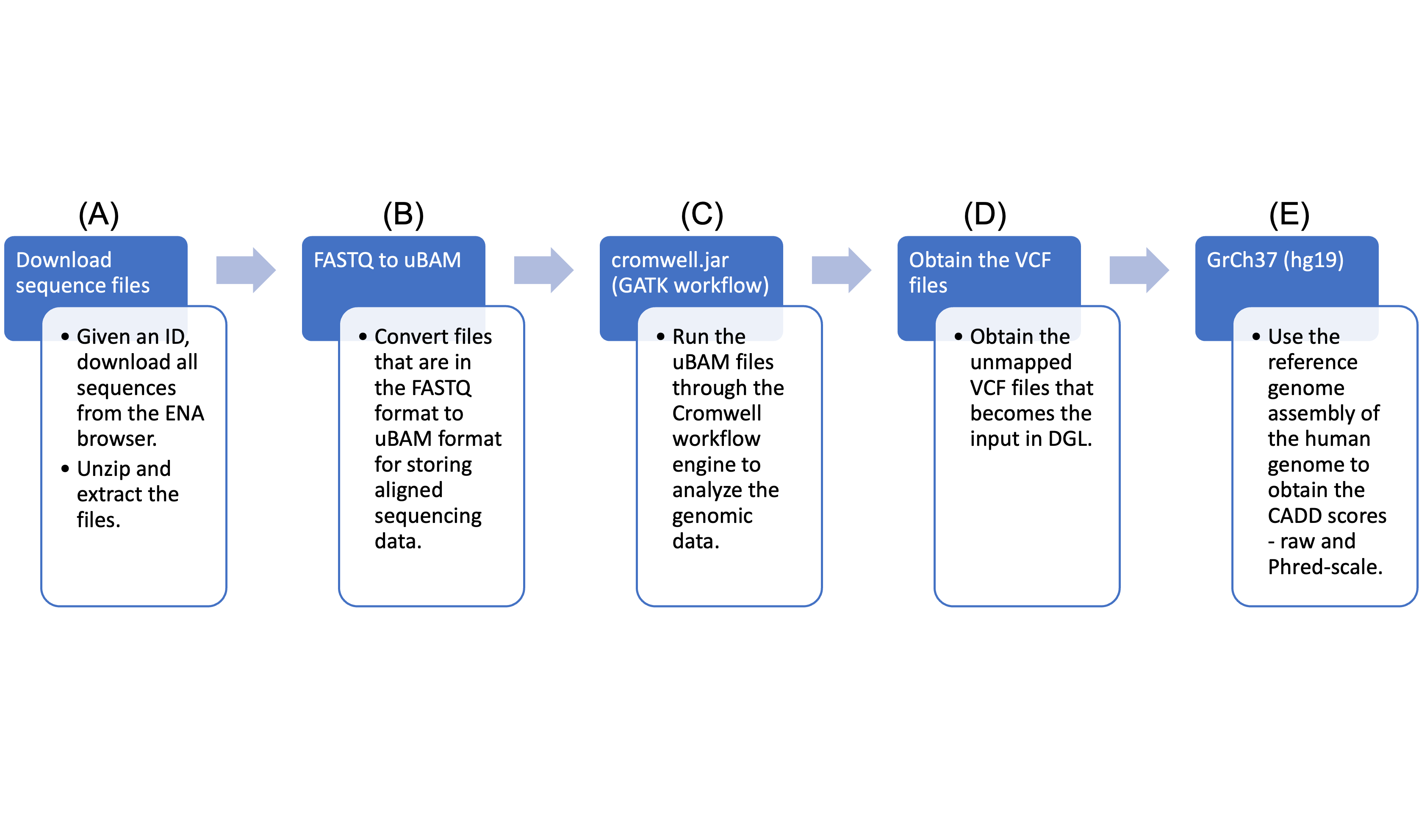
Figure 1: Workflow to show how the raw data was collected to be further processed and collated into a dataset.

• FASTQ files (part A): These IDs were utilized to download the RNA sequences, which were in FASTQ Li et al. (2008); Li and Durbin (2009) format. FASTQ is a text-based file format used for storing both a biological sequence (usually nucleotide sequence) and its corresponding quality scores. It is commonly used to represent the output of high-throughput sequencing technologies. The FASTQ file format consists of a series of records, each of which contains four lines of text: the first line starting with ‘@’ contains a sequence identifier, the second line contains the actual nucleotide sequence, the third line starts with ‘+’ and may optionally contain additional information about the sequence, and the fourth line contains quality scores encoded as ASCII 10 characters. The quality scores indicate the confidence in the accuracy of each base call and are typically represented as Phred scores.

• uBAM files (part B): The FASTQ files were then converted to unmapped BAM (uBAM) files for storing aligned sequencing data. It is an uncompressed version of a BAM file, which is a binary representation of sequence alignment data. A uBAM file contains unmapped reads, meaning reads that could not be confidently aligned to a reference genome. These reads can be used for downstream analysis, such as de novo assembly, quality control, and identification of novel sequences. Unlike a BAM file, a uBAM file does not contain alignment information and is, therefore smaller in size, making it more convenient for storage and transfer.

• GATK workflow (part C): The uBAM files were passed through the Genomic Analysis Toolkit (GATK) workflow McKenna et al. (2010) that converts the files into Variant Calling Format (VCF) Danecek et al. (2011) files. It is a comprehensive toolkit developed by the Broad Institute that includes various tools and algorithms for processing genomic data, such as read mapping, local realignment, base quality score recalibration, variant calling, and variant filtering. The workflow involves several steps, including preprocessing of raw data, alignment to a reference genome, post-alignment processing, and variant discovery and annotation.

• The unannotated VCF files that were obtained as the result of the workflow have been shown in part D. For each VCF file, there is also a corresponding CADD scores file that was obtained using GrCh37 through the workflow, as shown in part E.

3.2 Data Annotations

Once the RNA sequencing was completed, two main files were generated for each RNA-seq ID – a VCF file and a CADD scores file in TSV format.

For further annotations, SnpEff Cingolani et al. (2012), a command-line, variant annotation, and effect prediction tool, was utilized. This tool annotates and predicts the effects of genetic variants. SnpEff takes as input the predicted variants (SNPs, insertions, deletion, and MNPs) and produces a file with annotations of the variants and the effects they produce on known genes.

SnpEff classifies variants as single nucleotide polymorphisms (SNPs), insertions, deletions, multiple-nucleotide polymorphisms or an InDel. While the original VCF file contains the INFO field, SnpEff adds additional annotations to this field to further describe the variation. In the process, it also updates the header fields. This field is tagged by ‘ANN’, which is pipe symbol separated and provides a summary of the predicted effects of a genetic variant on each affected transcript. Figure 2 shows the ANN field highlighted in bold.

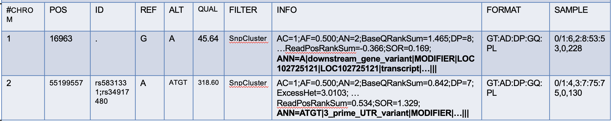
Figure 2: Additional annotations by the SnpEff tool.

A variant may have one or more annotations and multiple annotations are comma-separated. There are several fields within the ANN tag, mainly:

• Allele (ALT): Information on alternate alleles that are predicted to cause a functional impact on a gene or protein

• Annotation (effect): Type of effect caused by the variant on the transcript

• Putative impact: Qualitative measure of the impact of the variant on the transcript

• Gene name: Name of the affected gene

• Gene ID: Unique identifier of the affected gene

Ontology

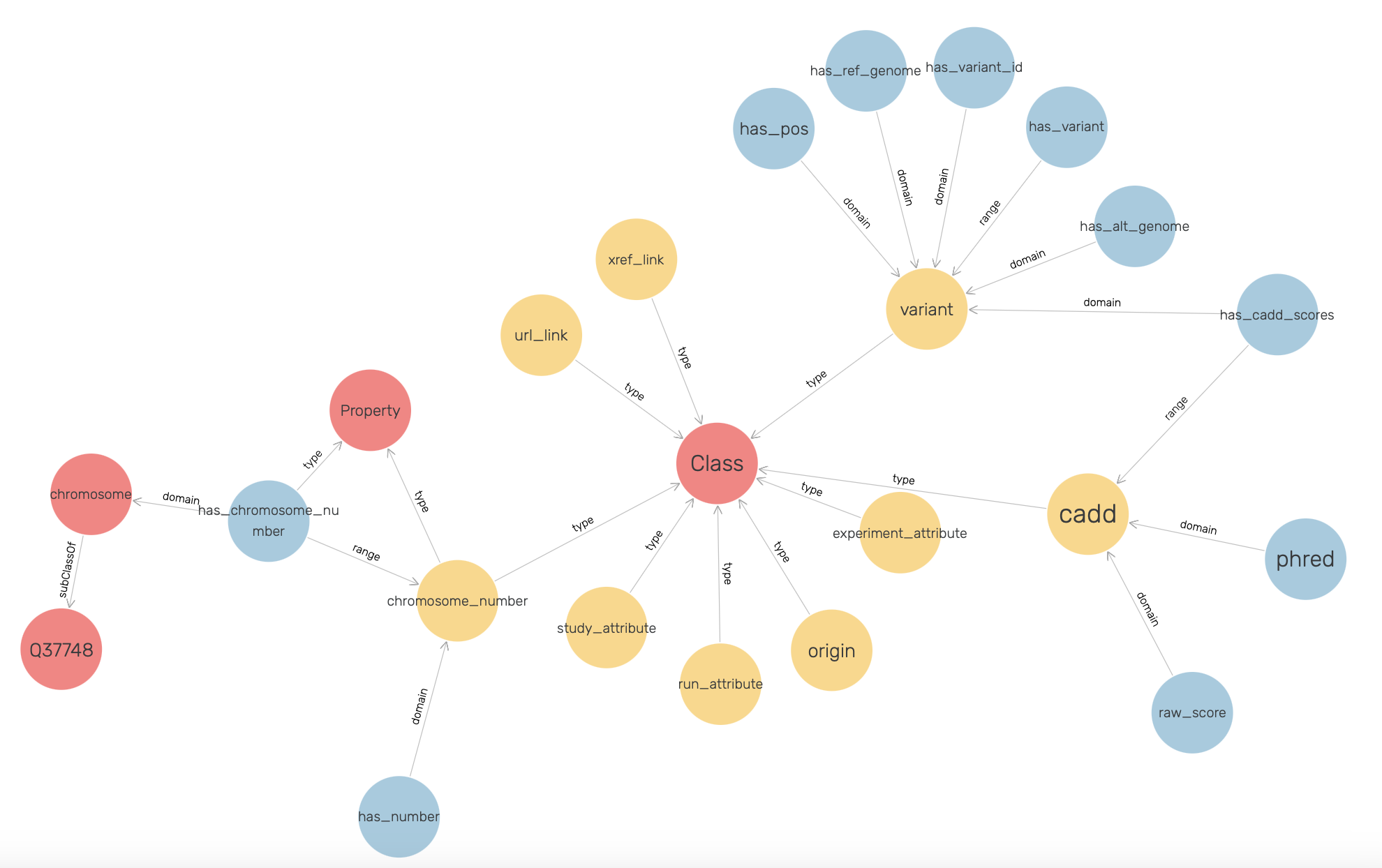
Figure 3: Ontology of the knowledge graph.

A knowledge graph is represented using an ontology, where the ontology can be represented using a formal language such as RDF (Resource Description Framework) or OWL (Web Ontology Language), or another domain-specific language. The ontology in this work has been represented using RDF. Each node-edge-node is represented as a triple by RDF. In a triple, the subject defines the first node, object defines the second node. The predicate defines the edge or relation joining the two nodes. A triple always ends with a dot.

An ontology mainly consists of classes, properties, and relationships. In Figure 3, the sub-classes are depicted by red nodes, the classes are by yellow nodes, and the relations by blue nodes. The description of the classes has been given in Table 1 and the description of the properties has been given in Table 2.

Table 1: Description of the classes in the ontology.

CLASS	DEFINITION
Chromosome Number	Identifier of the chromosome; values can be ‘1’, ‘2’, …, ‘22’, ‘X’, ‘Y’, ‘MT’
Origin	Unique identifier of the variant annotated by SPARQLing Genomics tool
Variant	Encapsulates the different types of genomic alterations that can occur
CADD	Encapsulates the different types of scores that can occur
xref_link	Type of annotation that provides a link between different resources or databases
url_link	Access link to experiment label
study_attribute	Metadata that describes the experimental design, data processing, and other aspects of a sequencing study
run_attribute	Metadata that describes the sequencing run
experiment_attribute	Metadata that describes the overall experimental design and goal of the experiment

Table 2: Description of the properties in the ontology.

PROPERTY	DEFINITION	DOMAIN	RANGE
has_pos	Variant position	Variant	Integer
has_ref_genome	Reference genome at that position	Variant	String
has_alt_genome	Alternate genome at that position	Variant	String
has_variant_id	Unique identifier of the variant	Variant	String
has_variant	Unique name given to the variant	Variant	String
has_cadd_scores	Variant has associated CADD scores	Variant	CADD
has_chromosome_number	Chromosome has a chromosome number	Chromosome	String
phred	Phred-scaled score	CADD	Long
raw_score	Raw CADD score	CADD	Long

In the defined ontology, chromosome and variant are both domain classes and a chromosome has an associated chromosome number to be able to connect all similar chromosomes as an extension, and a variant has an associated variant ID. A variant has a reference and alternate genome.

The ontology also explicitly defines CADD as a class where a variant has CADD scores represented by both raw score and Phred-scale score, as properties of the CADD class. The ontology description has been given in Table 3.

Table 3: Domain, properties, and ranges for the ontology.

ENTITY	RDF:PROPERTY	DOMAIN	RANGE
Chromosome	Type	N/A	Wiki:Q37748
	SubClassOf	N/A	Wiki:Q37748
has_chromosome_number	Type	N/A	Property
	Domain	Chromosome	N/A
	Range	chromosome_number	N/A
chromosome_number	Type	N/A	Class
has_number	Type	N/A	Property
	Domain	chromosome_number	N/A
	Range	xsd:int	N/A
Variant	Type	N/A	Class
has_variant	Type	N/A	Property
	Domain	Chromosome	Variant
	Range	Variant	N/A
has_pos	Type	N/A	Property
	Domain	Variant	xsd:string
	Range	xsd:int	N/A
has_ref_genome	Type	N/A	Property
	Domain	Variant	xsd:string
	Range	xsd:string	N/A
has_alt_genome	Type	N/A	Property
	Domain	Variant	xsd:string
	Range	xsd:string	N/A
CADD	Type	N/A	Class
has_cadd_score	Type	N/A	Property
	Domain	Variant	CADD
	Range	CADD	N/A
raw_score	Type	N/A	Property
	Domain	CADD	xsd:long
	Range	xsd:long	N/A
phred	Type	N/A	Property
	Domain	CADD	xsd:long
	Range	xsd:long	N/A

3.3 Conversion of VCF files to Knowledge Graphs

To transform the data in VCF, SPARQLing Genomics was utilized. SPARQLing Genomics is an open-source platform for querying and analyzing genomic data using the Semantic Web and Linked Data technologies. The platform provides an easy-to-use interface as well, that has been built to support SPARQL queries and various SPARQL query features, including sub-queries, filters, and aggregates. SPARQLing Genomics provides several in-built, ready-to-use tools, one of which is vcf2rdf that converts VCF data into RDF triples.

The triples generated by the tool consist of uniquely identifiable names having symbolic value and literal values like numbers or text.

⬇

#CHROM POS ID REF ALT QUAL FILTER INFO sample

1 16963 . G A 45.64 SnpCluster AC=1;AF=0.500;AN=2;BaseQRankSum=1.465;DP-8;ExcessHet=3.0103;FS=0.000;MLEAC=1;MLEAF=0.500;MQ=60.00;MQRankSum=0.000;QD=5.70;ReadPosRankSum=-0.366;SOR=0.169GT:AD:D:GQ:PL0/1:6,2:8:53:53,0,228

The following is an example of how a variant position (example shown above) is translated into a triple by the tool.

⬇

<origin://4a37140cdc877d90ffe258a8151f27e@0> <http://biohackathon.org/resource/faldo#position> "16963"^^<http://www.w3.org/2001/XMLSchema#integer> .

As seen in the above example, the variant position is described with Feature Annotation Location Description Ontology (FALDO) Bolleman et al. (2016). For other features not defined by FALDO, the URI is customized to the tool.

Each VCF file eventually corresponds to one large knowledge graph that was originally stored in an N3 format. N3 format is one of the several formats supported by RDF and can be considered as a shorthand non-XML serialization of RDF models. However, to accommodate the accessionID that would map to an unidentified patient, the N3 serialization was converted to NQ format with the accessionID as the named graph. An example of a triple from an N3 file has been given here.

⬇

<origin://4a37140cdc877d90ffe2b58a8151f27e@0> <sg://0.99.11/vcf2rdf/variant/REF> <sg://0.99.11/vcf2rdf/sequence/G> .

The triple was then converted to NQ format which yielded the following triple:

⬇

<origin://4a37140cdc877d90ffe2b58a8151f27e@0> <sg://0.99.11/vcf2rdf/variant/REF> <sg://0.99.11/vcf2rdf/sequence/G> <sg://SRR13112995>.

The ontology was extended to accommodate the new relations generated by the tool.

3.4 Conversion of CADD score files to Knowledge Graphs

The SnpEff and vcf2rdf tools were useful for converting VCF files to triples. However, CADD scores that were obtained through the pipeline were in tab-separated (TSV) format. To enrich the knowledge graphs, the CADD scores had to be translated to RDF triples as well. Therefore, the ontology for CADD scores was explicitly defined.

To visualize the graph, GraphDB has been utilized, and the ontology that was defined for CADD scores has been shown in Figure 4

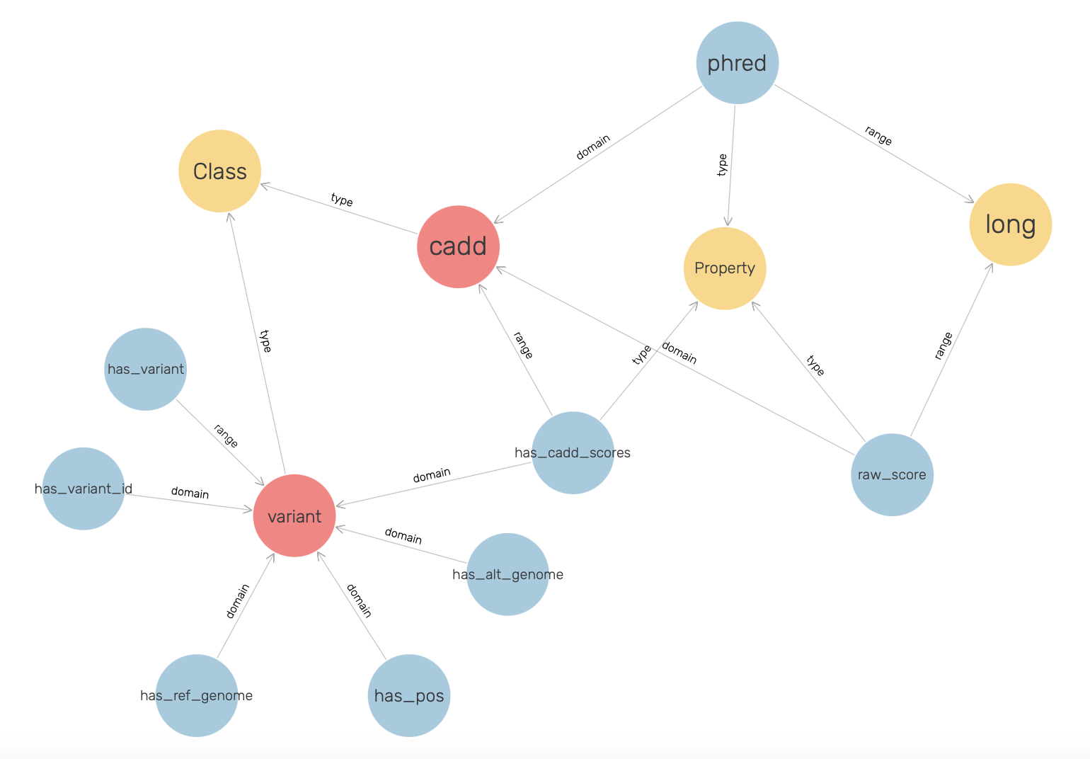
Figure 4: Ontology for CADD scores.

These scores have been represented with respect to the described fields in the VCF files such as the chromosome, position, reference genome, and alternate genome. The raw scores and Phred-scale scores were obtained from the original TSV files.

The following is an example of a record in a TSV file for which the raw and phred scores map to chromosome 1 with position 16963, reference genome ‘G’ and alternate genome ‘A’ in the VCF file:

#Chrom	Pos	Ref	Alt	RawScore	PHRED
1	16963	G	A	0.900784	12.72

Each data record, like the above example, was converted to a Turtle triple (TTL), another format supported by RDF. A TTL format writes a graph in a compact textual form. There are only 3 parts to this triple – subject, predicate, and object. An example of the above data record converted to a TTL triple is given below:

⬇

<http://sg.org/SRR13112995/1/variant1> a ns1:variant ;

ns1:has_alt_genome "A" ;

ns1:has_cadd_scores <http://sg.org/SRR13112995/1/variant1/cadd> ;

ns1:has_pos 16963 ;

ns1:has_ref_genome "G" .

4 Results

Each variant file represented a single knowledge graph, so to unify several knowledge graphs into one single large graph, BlazeGraph Database has been leveraged. This large knowledge graph was then queried to create a dataset for a case study. It is important to note that the edges are homogeneous in nature.

BlazeGraph is a high-performance, horizontally scalable, and open-source graph database that can be used to store and manage large-scale graph data. It has been designed to provide efficient graph querying and supports RDF data model that allows it to store and process both structured and semi-structured data. BlazeGraph uses a distributed architecture that can be easily integrated with other big data tools, such as Hadoop and Spark, to perform complex analytics on large-scale graph data.

BlazeGraph has been leveraged for efficiently querying the knowledge graphs to generate the dataset for Graph Neural Network downstream tasks. Other tools such as RIQ Katib et al. (2017, 2016); Slavov et al. (2015) can be used to index and query RDF named graphs.

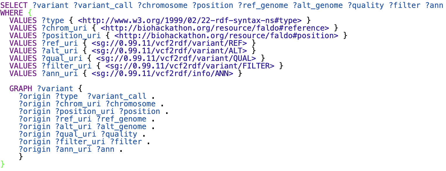
Figure 5: SPARQL query to extract variant and its properties.

The total number of triples in the knowledge graph, after aggregating only 511 VCF files on a single machine, is as large as 3.1 Billion.

To query the variant that has properties such as chromosome, position, reference, and alternate genomes and the ANN field that had been annotated by the SnpEff tool, the SPARQL query in Figure 5 was used.

Each chromosome has a position that has an associated reference genome, alternate genome, quality, and filter.

5 KG INFERENCE: CASE STUDY

In this section, we will discuss a case study using the created knowledge graph. We aim to use the KG for a classification task using graph machine learning. The objective of the task is to classify a variant (or a node) into a CADD score category, given information about the variant. These categories allow researchers to identify where the actual raw score may lie for the variant. This would allow researchers to focus on the more likely deleterious variants first, depending on the nature of the problem.

For the classification task, we are leveraging the open-source graph-based library called Deep Graph Library Wang et al. (2019).

5.1 Deep Graph Library

To implement the task, Deep Graph Library (DGL), an open-source library supporting graph-based deep learning was utilized. DGL provides a set of high-level APIs for building scalable and efficient graph neural network models. With DGL, we can create, manipulate, and learn from large-scale graphs with billions of nodes and edges.

There are three main tasks supported by DGL:

• Node Classification: Predict the class or label of a node in a graph based on its features.

• Link Prediction: Predict if there is a connection or an edge between two nodes.

• Graph Classification: Classify an entire graph into one or more classes or categories.

DGL represents a graph as a DGLGraph object, which is a framework-specific graph object. It requires the number of nodes and a list of source and destination nodes, where nodes and edges must have consecutive IDs starting from 0. Since DGL only accepts numeric input, all strings such as URI were mapped to integers. In this case study, node classification was used to classify variants into CADD score categories based on their features.

5.2 Subset Graph Transformation

The knowledge graph created needs to be transformed into the input required by DGL due to its design specifications. The transformation of the input required for graph machine learning needs to be done in a scalable and efficient way.

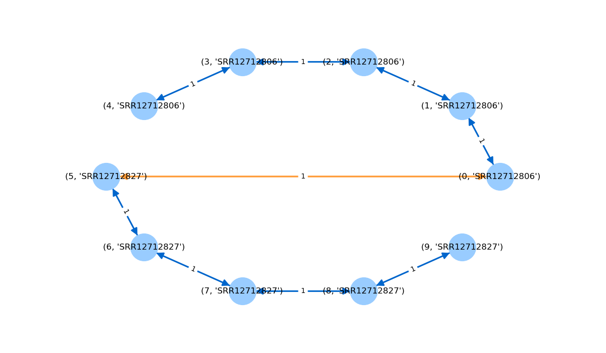
Figure 6: Graph where every raw variant ID is connected, within the same accession ID, as depicted by blue bidirectional arrows. Orange bidirectional arrow depicts two nodes connected across accession ID, by a shared variant ID.

The graph was transformed in a way that all nodes belonging to the same accession ID or patient shared an edge and all nodes that share a variant ID also shared an edge. With this, no two nodes within the same accession ID can share a variant ID as this is unique to the accession ID. Therefore, nodes that share a variant ID are connected across accession IDs. This has been shown in Figure 6.

For the task, a portion of the graph was extracted as a projection where SPARQL queries were used to prepare the subset of the graph dataset that now contains variants connected to each other by a variant ID. That is, two nodes share an edge between them if they belong to the same variant ID. This projection has been shown in Figure 7 and the node features for a sample node have been shown in Figure 8.

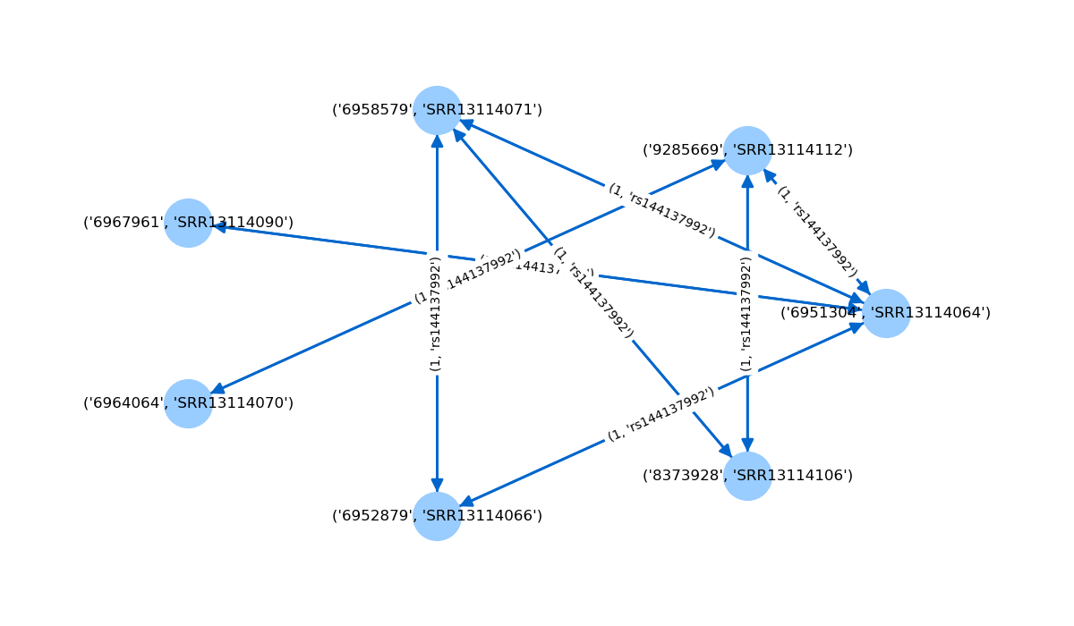
Figure 7: Projection of a denser graph where two nodes are connected if they share a variant ID.

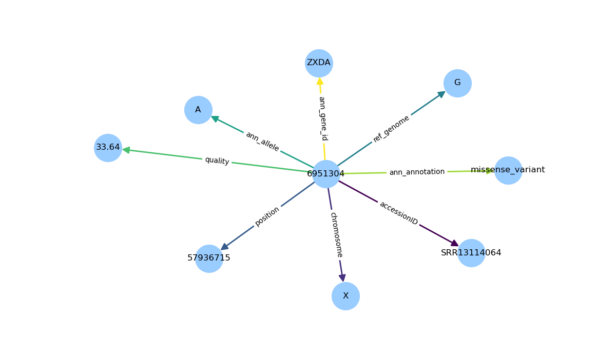
Figure 8: Node features of a sample node.

As in Figure 8, the accession ID, chromosome, position, reference genome, alternate genome, quality, and ANN information such as allele, annotation, gene name, and gene ID were considered as the node features.

The subset graph contained 190 unique accession IDs, with 73,661,245 nodes and 112,707,621 edges.

5.3 Node Classification Task

For this task, Graph Convolutional Network (GCN) Zhang et al. (2019) and GraphSAGE Hamilton et al. (2017) have been used. For both models, each node is associated with a feature vector.

GCNs use node embeddings and adjacency matrices to compute new embeddings while training. Similar to CNN, the model weights and biases are first initialized to 1, and then a section of the graph is passed through the model. A non-linear activation function is used to compute predicted node embeddings for each node. Cross entropy loss is calculated to quantify the difference between the predicted node embeddings and the ground truth. Loss gradients are then computed to update the model using the Adam optimizerKingma and Ba (2014) for this task. These steps are repeated until convergence.

GraphSAGE uses SAGEConv layers where for every iteration, the output of the model involves finding new node representation for every node in the graph. Mean is used as the aggregation function and ReLU activation function has been utilized. Adam optimizer was used for this model as well. One of the most noted properties of GraphSAGE is its ability to aggregate neighbor node embeddings for a given target node. Through the experiments conducted, this property was observed. GraphSAGE also generalizes better to unseen nodes because of its ability to perform inductive learning on graphs.

The CADD (raw) scores have been categorized into 5 categories of equal distribution, primarily based on their frequencies generating target labels from 0 to 5. These categories have been shown in Table 4. The categories or bins for the target labels are based on the pattern found in the raw data used in this work. The categories are not arbitrary because there are no pre-defined CADD score categories.

Table 4: CADD score categories for the classification task.

RAW SCORES RANGE	CATEGORY
Less than 0	0
0-1	1
1-5	2
5-10	3
10-100	4

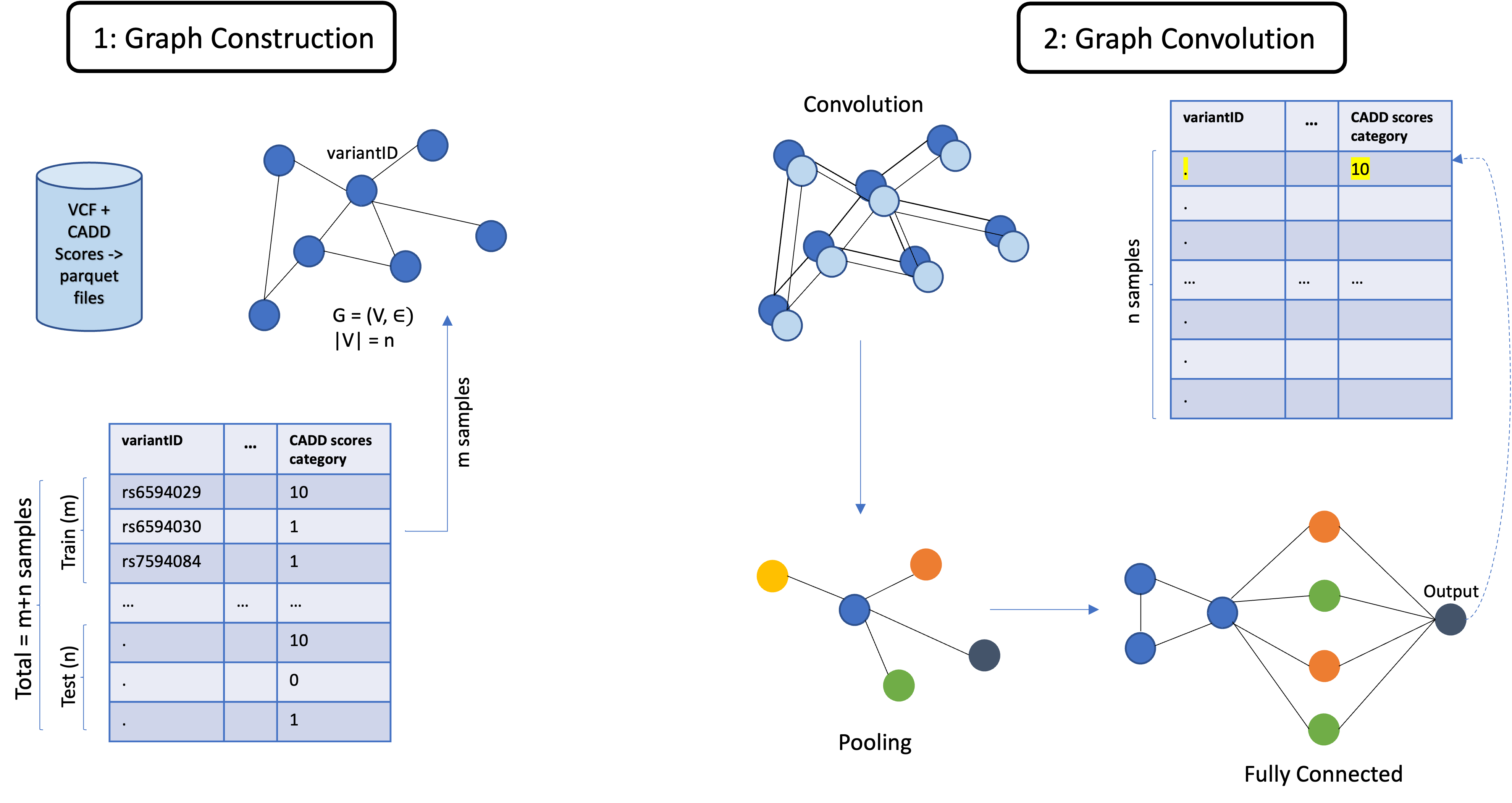
Figure 9: Architecure of GCN.

The architecture of GCN has been shown in Figure 9. The architecture of GraphSAGE differs in the property of message passing between the nodes. This was crucial as the nodes in the input graph relied on several pieces of information from their neighboring nodes.

5.4 Experiments & Results

5.4.1 Experiment Setup

The experiments were run on CloudLab , a testbed for cloud computing research and new applications. CloudLab cluster at Clemson University was built in partnership with Dell. Clemson machines were used to carry out the standalone training experiments. They were carried out on nodes with 16 cores per node (2 CPUs), 12x4 TB disk drives in each node, plus 8x1 TB disks in each node. The nodes are configured with 256 GB of memory and 73TB of RAM. The operating system installed across all of them was Ubuntu 18.04.

Wisconsin machines were also used to carry out the standalone training experiments described in section 6.2. The CloudLab cluster at the University of Wisconsin was built in partnership with Cisco, Seagate, and HP. The cluster has 523 servers with a total of 10,060 cores and 1,396 TB of storage, including SSDs on every node.

The nodes were chosen upon availability for the standalone node classification tasks.

5.4.2 Experiment Results

The data input was a graph with 73,661,245 nodes or vertices and 112,707,621 edges from 190 variants. The data was split into 60:20:20 (train:val:test) ratio and Graph Convolutional Network (GCN) and GraphSAGE models were used to train on this dataset in separate experiments. Adam optimizer was employed along with Cross Entropy loss in both models. Grid search was conducted to find the most optimum hyperparameters.

Table 5 shows the hyperparameter tuning results for GraphSAGE and GCN models. For GraphSAGE, hyperparameter tuning was conducted keeping the learning rate of 0.001 constant over 1500 epochs with variable number of hidden layers. The hidden layers were chosen from 2, 8, 16, and 32 and it was observed that the highest validation accuracy of 85.8% was observed when the model had 32 hidden layers. Similar experiments were performed on the GCN model, and it was observed that this model, too, yielded the highest validation accuracy of 84% for 32 hidden layers. The best models in both sets of experiments were then evaluated on the test set, giving 86.67% test accuracy by GraphSAGE and 82.6% test accuracy by GCN.

Table 5: Performance comparison of GraphSAGE and GCN. The test accuracy is only computed for models with the best validation set accuracy. HL = Hidden Layers; LR = Learning Rate; VAL = Validation Accuracy; TEST = Test Accuracy

HL	LR = 0.001
	GraphSAGE		GCN
	VAL	TEST	VAL	TEST
2	22.9	-	22.7	-
8	72.8	-	61.3	-
16	84.7	-	72.4	-
32	85.8	86.67	84	82.6

The confusion matrices for the best models on the test set are shown in Figures 10(a) and 10(b).

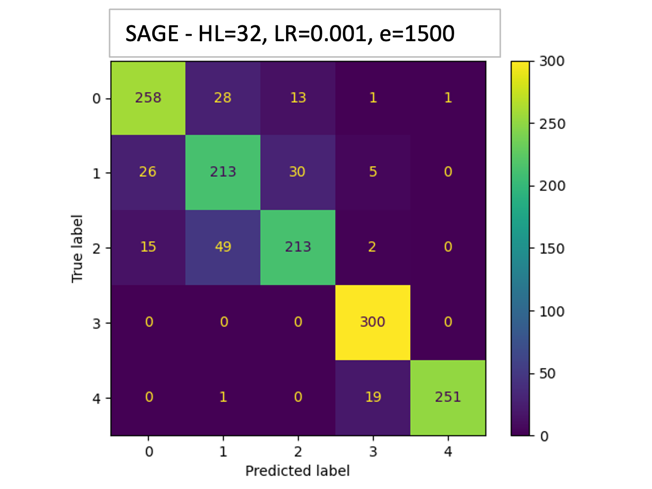
(a)

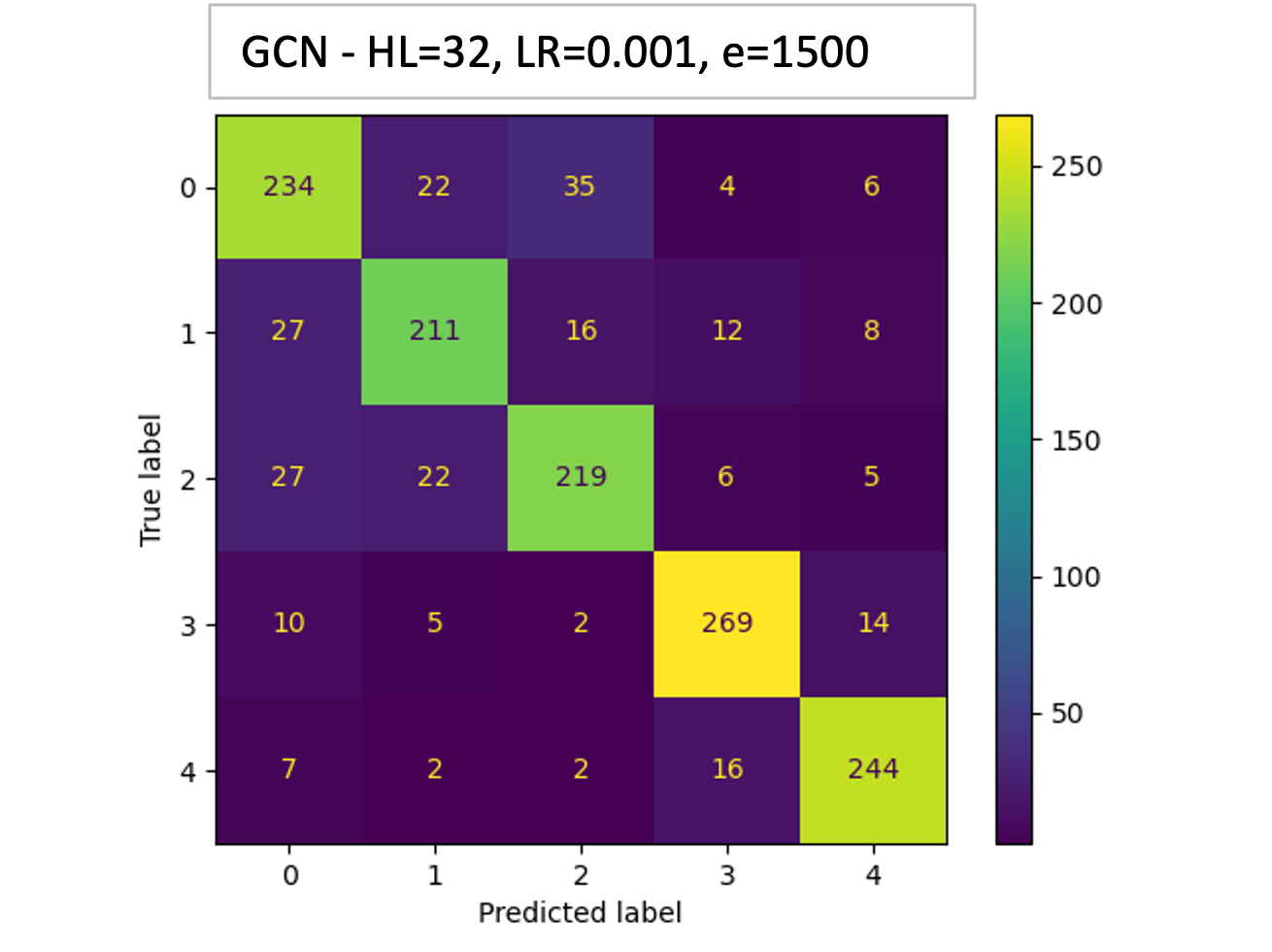
(b)

Figure 10: Confusion matrices for (a) GraphSAGE model and (b) GCN model that yielded the highest test accuracy.

Another set of experiments of a similar nature, shown in Table 6, were conducted keeping the learning rate constant at 0.01 over 1000 epochs with the same set of hidden layers hyperparameter values. It was observed that the highest validation accuracy for GraphSAGE was 91.5% with 16 hidden layers and for GCN was 84% with 32 hidden layers. The best models in these experiments were then evaluated on the test set, giving 91.02% test accuracy by GraphSAGE over 74.88% test accuracy by GCN.

Table 6: Performance comparison of GraphSAGE and GCN. The test accuracy is only computed for models with the best validation set accuracy. HL = Hidden Layers; LR = Learning Rate; VAL = Validation Accuracy; TEST = Test Accuracy

HL	LR = 0.01
	GraphSAGE		GCN
	VAL	TEST	VAL	TEST
2	21.5	-	21.5	-
8	37.9	-	60.7	-
16	91.5	91.02	81.1	-
32	83.1	-	84	74.88

The confusion matrices for the best models on the test set are shown in Figures 11(a) and 11(b). GraphSAGE model with 16 hidden layers and a learning rate of 0.01 gave the highest test accuracy of 91.02% across all the experiments conducted.

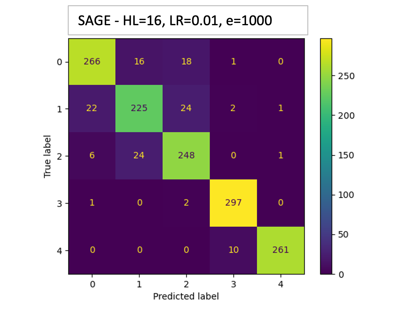
(a)

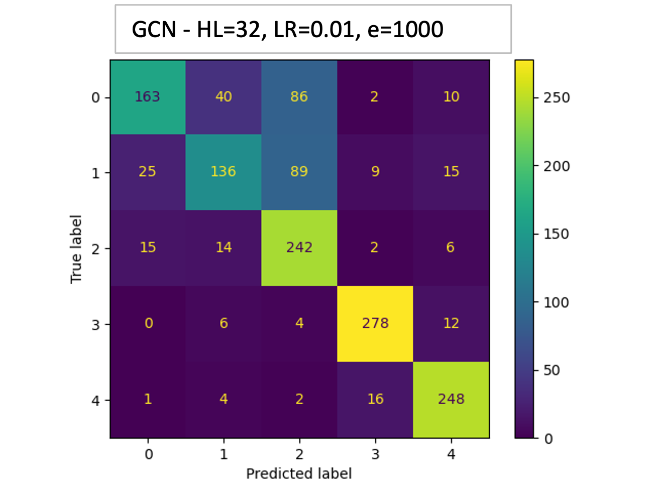
(b)

Figure 11: Confusion matrices for (a) GraphSAGE model and (b) GCN model that yielded the highest test accuracy.

6 Conclusion

This work shows that representing genomic data as knowledge graphs allows vast and diverse information to be integrated from various sources. Modeling entities as nodes and relationships as edges provides an ideal framework for integrating and organizing diverse information. We first described the data collection pipeline followed by the usage of the SnpEff tool to obtain additional annotations and SPARQLing Genomics tool to convert the annotations to an RDF format. An ontology to collate information gathered from different sources is presented. Using this ontology, we described how the knowledge graph is created. This knowledge graph contains RNA sequencing information at the variant level from COVID-19 patients from different regions such as lung, blood, etc. Lastly, we presented a case study to demonstrate the usage of the created knowledge graph for a node classification task using the Deep Graph Library. As part of this case study, we also described various experiments that were performed, the corresponding results, and discussed key observations. As part of our future work, we aim to expand the knowledge graph and explore more avenues to use the same to aid researchers working in this domain.

7 Acknowledgments

This work was supported by the National Science Foundation under Grant Nos. 2201583 and 2034247.

References

- Rentzsch et al. [2019] Philipp Rentzsch, Daniela Witten, Gregory M Cooper, Jay Shendure, and Martin Kircher. Cadd: predicting the deleteriousness of variants throughout the human genome. Nucleic acids research, 47(D1):D886–D894, 2019.
- Rentzsch et al. [2021] Philipp Rentzsch, Max Schubach, Jay Shendure, and Martin Kircher. Cadd-splice—improving genome-wide variant effect prediction using deep learning-derived splice scores. Genome medicine, 13(1):1–12, 2021.
- Rao et al. [2021] Praveen Rao, Arun Zachariah, Deepthi Rao, Peter Tonellato, Wesley Warren, and Eduardo Simoes. Variant analysis of human genome sequences for covid-19 research. 2021. doi:10.21227/b0ph-s175. URL https://dx.doi.org/10.21227/b0ph-s175.
- Feng et al. [2023] Fan Feng, Feitong Tang, Yijia Gao, Dongyu Zhu, Tianjun Li, Shuyuan Yang, Yuan Yao, Yuanhao Huang, and Jie Liu. Genomickb: a knowledge graph for the human genome. Nucleic Acids Research, 51(D1):D950–D956, 2023.
- Reese et al. [2021] Justin T Reese, Deepak Unni, Tiffany J Callahan, Luca Cappelletti, Vida Ravanmehr, Seth Carbon, Kent A Shefchek, Benjamin M Good, James P Balhoff, Tommaso Fontana, et al. Kg-covid-19: a framework to produce customized knowledge graphs for covid-19 response. Patterns, 2(1), 2021.
- Harnoune et al. [2021] Ayoub Harnoune, Maryem Rhanoui, Mounia Mikram, Siham Yousfi, Zineb Elkaimbillah, and Bouchra El Asri. Bert based clinical knowledge extraction for biomedical knowledge graph construction and analysis. Computer Methods and Programs in Biomedicine Update, 1:100042, 2021. doi:https://doi.org/10.1016/j.cmpbup.2021.100042.
- Liu et al. [2020] Qiao Liu, Zhiqiang Hu, Rui Jiang, and Mu Zhou. Deepcdr: a hybrid graph convolutional network for predicting cancer drug response. Bioinformatics, 36(Supplement_2):i911–i918, 2020. doi:https://doi.org/10.1093/bioinformatics/btaa822.
- Lanchantin and Qi [2019] Jack Lanchantin and Yanjun Qi. Graph convolutional networks for epigenetic state prediction using both sequence and 3d genome data. BioRxiv, page 840173, 2019. doi:https://doi.org/10.1101/840173.
- Sun et al. [2018] Wenli Sun, Changgee Chang, Yize Zhao, and Qi Long. Knowledge-guided bayesian support vector machine for high-dimensional data with application to analysis of genomics data. In 2018 IEEE International Conference on Big Data (Big Data), pages 1484–1493. IEEE, 2018.
- Li et al. [2008] Heng Li, Jue Ruan, and Richard Durbin. Mapping short dna sequencing reads and calling variants using mapping quality scores. Genome research, 18(11):1851–1858, 2008.
- Li and Durbin [2009] Heng Li and Richard Durbin. Fast and accurate short read alignment with burrows–wheeler transform. bioinformatics, 25(14):1754–1760, 2009.
- McKenna et al. [2010] Aaron McKenna, Matthew Hanna, Eric Banks, Andrey Sivachenko, Kristian Cibulskis, Andrew Kernytsky, Kiran Garimella, David Altshuler, Stacey Gabriel, Mark Daly, et al. The genome analysis toolkit: a mapreduce framework for analyzing next-generation dna sequencing data. Genome research, 20(9):1297–1303, 2010.
- Danecek et al. [2011] Petr Danecek, Adam Auton, Goncalo Abecasis, Cornelis A Albers, Eric Banks, Mark A DePristo, Robert E Handsaker, Gerton Lunter, Gabor T Marth, Stephen T Sherry, et al. The variant call format and vcftools. Bioinformatics, 27(15):2156–2158, 2011.
- Cingolani et al. [2012] P. Cingolani, A. Platts, M. Coon, T. Nguyen, L. Wang, S.J. Land, X. Lu, and D.M. Ruden. A program for annotating and predicting the effects of single nucleotide polymorphisms, snpeff: Snps in the genome of drosophila melanogaster strain w1118; iso-2; iso-3. Fly, 6(2):80–92, 2012.
- Bolleman et al. [2016] Jerven T Bolleman, Christopher J Mungall, Francesco Strozzi, Joachim Baran, Michel Dumontier, Raoul JP Bonnal, Robert Buels, Robert Hoehndorf, Takatomo Fujisawa, Toshiaki Katayama, et al. Faldo: a semantic standard for describing the location of nucleotide and protein feature annotation. Journal of biomedical semantics, 7(1):1–12, 2016.
- Katib et al. [2017] Anas Katib, Praveen Rao, and Vasil Slavov. A Tool for Efficiently Processing SPARQL Queries on RDF Quads. In International Semantic Web Conference (Posters, Demos & Industry Tracks), 2017.
- Katib et al. [2016] Anas Katib, Vasil Slavov, and Praveen Rao. RIQ: Fast processing of SPARQL queries on RDF quadruples. Journal of Web Semantics, 37-38:90–111, 2016. ISSN 1570-8268.
- Slavov et al. [2015] Vasil Slavov, Anas Katib, Praveen Rao, Srivenu Paturi, and Dinesh Barenkala. Fast processing of SPARQL queries on RDF quadruples. arXiv preprint arXiv:1506.01333, 2015.
- Wang et al. [2019] Minjie Wang, Da Zheng, Zihao Ye, Quan Gan, Mufei Li, Xiang Song, Jinjing Zhou, Chao Ma, Lingfan Yu, Yu Gai, Tianjun Xiao, Tong He, George Karypis, Jinyang Li, and Zheng Zhang. Deep graph library: A graph-centric, highly-performant package for graph neural networks. arXiv preprint arXiv:1909.01315, 2019.
- Zhang et al. [2019] Si Zhang, Hanghang Tong, Jiejun Xu, and Ross Maciejewski. Graph convolutional networks: a comprehensive review. Computational Social Networks, 6(1):1–23, 2019.
- Hamilton et al. [2017] Will Hamilton, Zhitao Ying, and Jure Leskovec. Inductive representation learning on large graphs. In Advances in neural information processing systems, page 30.d, 2017.
- Kingma and Ba [2014] Diederik P Kingma and Jimmy Ba. Adam: A method for stochastic optimization. arXiv preprint arXiv:1412.6980, 2014.