Finite-Temperature Simulations of Quantum Lattice Models with Stochastic Matrix Product States

Abstract

In this work, we develop a stochastic matrix product state (stoMPS) approach that combines the MPS technique and Monte Carlo samplings and can be applied to simulate quantum lattice models down to low temperature. In particular, we exploit a procedure to unbiasedly sample the local tensors in the matrix product states, which has one physical index of dimension $d$ and two geometric indices of dimension $D$, and find the results can be continuously improved by enlarging $D$. We benchmark the methods on small system sizes and then compare the results to those obtained with minimally entangled typical thermal states, finding that stoMPS has overall better performance with finite $D$. We further exploit the MPS sampling to simulate long spin chains, as well as the triangular and square lattices with cylinder circumference $W$ up to 4. Our results showcase the accuracy and effectiveness of stochastic tensor networks in finite-temperature simulations.

I Introduction

Finite-temperature calculations of quantum many-body system play an indispensable role in the studies of quantum matter and materials. It bridges the gap between quantum lattice models and experiments in a wide range of investigations, ranging from studies of highly frustrated quantum magnets, unconventional superconductivity, to the ultracold atom quantum simulations. In frustrated quantum magnets, the finite-temperature approach can help determine the microscopic spin models from fitting the measured thermodynamic properties [1, 2, 3, 4, 5], including the specific heat, magnetic susceptibility, and also spin dynamics at finite temperature, providing insight into the quantum spin states in the compounds [1, 2, 3, 6, 7, 8]. It can also be exploited to study the exotic low-temperature electron states in the fermion Hubbard model [9, 10, 11, 12], enabling an unbiased and accurate comparison with optical lattice quantum simulations [13, 14, 15].

Tensor networks offer a feasible method for partially overcoming the exponential wall in quantum many-body simulations. Beyond the ground-state properties, various thermal tensor-network algorithms were proposed for accurate finite-$T$ calculations [16, 17, 18, 19, 20, 21, 22, 23, 24, 25, 26, 27, 28, 29, 30]. Currently, the finite-$T$ tensor-network methods can be classified into two major categories, purification and typical thermal states. The former exploits tensor-network representations, e.g., matrix product operator (MPO) and projected entangled pair operator (PEPO), of the thermal density matrix, and can be used to simulate both 1D and 2D systems [16, 17, 18, 20, 19, 20, 23, 24, 26, 27, 28, 29, 30]. The latter, with a representative method called minimally entangled typical thermal states (METTS) [31, 22, 32, 33, 9, 34], constructs a Markov chain samplings of matrix product state (MPS) [35, 36] with very short self-correlation length.

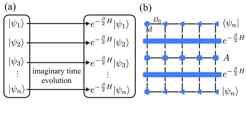
Figure 1: In the stoMPS algorithm, we (a) sample the isometric MPS $|{\psi_{n}}\rangle$ in a given sample space, and (b) calculate the expectation values of quantity $A$ on the time-evolved MPS $e^{-\frac{\beta}{2}H}|{\psi_{n}}\rangle$.

Both approaches have their own pros and cons. The MPO-based approaches benefits from the high precision and controllability in 1D and quasi-1D systems with certain widths $W$. The local tensor in MPO have two physical indices, different from that of the MPS with a single physical index. At sufficiently low temperature, the geometric bond dimension of MPO is also believed to be significantly larger than that in the ground-state MPS. Therefore, it is a nice idea switching from MPO to MPS to improve the efficiency in the low-temperature limit [31, 22]. However, in practical calculations of both 1D and 2D lattice systems, it has been demonstrated that MPS-based Monte Carlo sampling, such as that used in METTS, is still less efficient and less accurate than the MPO-based approach [25, 28, 29, 30]. Therefore, there is still a great need to develop more efficient stochastic MPS methods to further enhance the performance of this hybrid approach that combines tensor networks and Monte Carlo sampling.

In this work, we introduce a highly efficient stochastic matrix product state (stoMPS) approach inspired by the finite-temperature Lanczos method (FTLM) [37, 38, 39], which is used for evaluating systems of small sizes. FTLM combines the Lanczos diagonalization technique with random sampling and converting the problem of diagonalizing the Hamiltonian in the full Hilbert space to the Krylov subspace generated from some random initial states. We device the stoMPS algorithm as a generalization of FTLM and make detailed comparisons between results obtained with several different sample spaces. We find that sampling in a continuous sample space shows better performance, even outperforming the METTS method with Markov-chain sampling. Furthermore, we demonstrate the high scalability of this approach by applying it on 2D cylinders with width up to $W=4$. The connections of our stoMPS approach to the thermal pure quantum (TPQ) states [40, 41, 42, 43] are also discussed.

The rest part of the article is arranged as follows. In Sec. II we introduce the stoMPS algorithm and compare it to FTLM as well as METTS methods. The applications of stoMPS approach to 1D spin chains, square, and triangular lattice Heisenberg models are presented in Sec. III, and Sec. IV is devoted to the summary.

II Stochastic Matrix Product State Algorithm

II.1 Sampling Algorithm with Matrix Product States

The stoMPS workflow is depicted in Fig. 1, which is a tensor-network generalization of FTLM to large system size. In the FTLM method (see Appendix A), a random vector is uniformly selected from the unit sphere of the many-body Hilbert space $\mathcal{H}$ as the starting point, and a Krylov space is constructed based on this initial state. The total Hamiltonian is then projected into this subspace using the Lanczos technique, and the average value is computed. By repeating this process, one can obtain the finite-temperature properties of many-body systems, despite limitations in system size, with high accuracy [37, 38, 39].

To extend this approach to larger systems, we resort to stochastic MPS states instead of random initial vectors. A crucial question that needs to be addressed for this generalization is how to perform MPS samplings in a manner that represents the unit sphere unbiasedly. It is notable that with any given sample space $\{|{\psi}\rangle\}\subset{\mathcal{H}}$, we have

$$A(\beta):=\frac{{\rm\tr}[e^{-\beta H}A]}{{\rm\tr}[e^{-\beta H}]}=\frac{\mathbb{E}\left[\bra{\psi}e^{-\beta H}A|{\psi}\rangle\right]}{\mathbb{E}\left[\bra{\psi}e^{-\beta H}|{\psi}\rangle\right]},$$ (1)

for an observable $A$ if and only if a proper probability is chosen, such that the expectation satisfies

$$\mathbb{E}\left[|{\psi}\rangle\bra{\psi}\right]\propto I,$$ (2)

where $\beta$ is the inverse temperature, and $I$ is the identity in the Hilbert space.

One way to make $|{\psi}\rangle$ satisfy condition Eq. (2) is to restrict the sample space to the subset of all direct product states ($D=1$ MPS), which simplifies the condition to a local version, i.e., $\mathbb{E}\left[|{s_{i}}\rangle\bra{s_{i}}\right]\propto I_{\mathcal{H}_{i}}$ for each site $i$, where $\mathcal{H}_{i}$ is the local Hilbert space and $I_{\mathcal{H}_{i}}$ is the identity operator. Specifically, we can let $|{s_{i}}\rangle$ distribute uniformly on $\{\uparrow,\downarrow\}$ (dubbed as $Z_{2}$ sampling hereafter) or on the unit sphere [dubbed as U(1) sampling], which is equivalent to the $D=1$ case of the random isometry sampling introduced below for general $D\geq 1$ cases), i.e., $|{s_{i}}\rangle=\cos\theta|{\uparrow}\rangle+\sin\theta|{\downarrow}\rangle$, where $\theta\sim{\rm U}[0,2\pi]$ for spin-1/2 systems with local Hilbert space dimension $d=2$.

Note the physical meaning of the isometric local tensors of a canonical MPS can be understood as the sequentially selected renormalization basis. Inspired by this, we can naturally generalize the sampling from $Z_{2}$ and U(1) to the $A$ tensor in MPS with finite $D$. We sample random isometries and require the final center tensor distribute uniformly on the unit sphere of local renormalized Hilbert space. We find it is sufficient to satisfy Eq. (2) if the isometries distributed on Stiefel manifold St($D,Dd$) according to the Haar measure and are independent amongst different sites. The expectation $\mathbb{E}\left[|{\psi}\rangle\bra{\psi}\right]$ can be decomposed from site to site, then one can find the total tensor network represents an identity via recursively using a lemma on random isometry (see Appendix B) from the left to the right, see Fig. 2(c).

To be practical, the random isometries are generated via QR decomposition of a $D\times d\times D$ random tensor where each element is generated independently according to standard normal distribution $\mathcal{N}(0,1)$ [45, 46], c.f. Fig. 2(b). Besides the sampling scheme shown in Fig. 2, there exists an alternative approach to obtain the initial MPS from random unitary MPO [see Appendix C and also Ref. [40]].

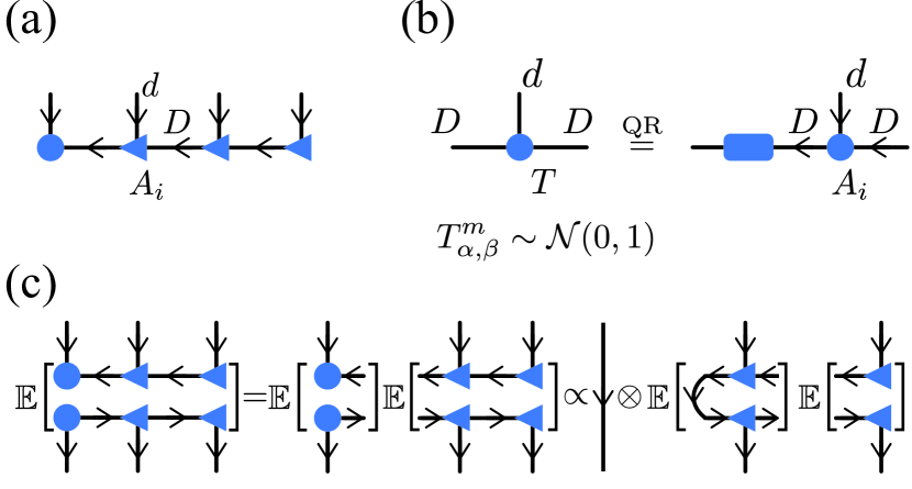
Figure 2: (a) The construction of stochastic isometric MPS, which satisfies the canonical condition following the order specified by the arrows. (b) To sample the isometric MPS, we conduct QR decomposition of the random matrix $T_{\alpha,\beta}^{m}$ whose elements are independently generated according to the standard normal distribution $\mathcal{N}(0,1)$. (c) The expectation of $|{\psi}\rangle\bra{\psi}$ in MPS representation, which can be reduced sequentially into product of identity, and thus satisfy Eq. (2).

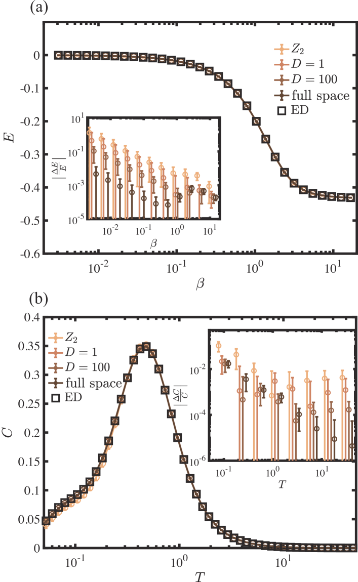
Figure 3: The energy and specific heat results of the $L=16$ Heisenberg chain. (a) shows the the energy results, where various sampling schemes generate results in excellent agreement with ED. The inset shows the statistical errors, which are very small and continuously improved as the initial bond dimension $D$ increases, approaching the results of FTLM with equivalently full rank $D$. (b) shows the specific heat results, where the inset shows that the standard errors also decrease with $D$.

II.2 Benchmark on the Heisenberg Spin Chain

Below we showcase the accuracy and efficiency of the stoMPS approach with different sampling schemes on a $L=16$ Heisenberg chain with XXZ Hamiltonian

$$H=\sum_{i}J_{xy}(S_{i}^{x}S_{i+1}^{x}+S_{i}^{y}S_{i+1}^{y})+J_{z}S_{i}^{z}S_{i+1}^{z}.$$

The calculated energy and heat capacity with corresponding stand errors are shown in Fig. 3. At low temperatures, the $Z_{2}$ sampling performs poorly, as the overlap between the initial state and the ground state vanishes when $\langle S^{z}_{\rm tot}\rangle\neq 0$ initial state is selected randomly. However, as $D$ increases we find the mean value approaches the ED results, with stand errors of energy expectation $\sigma[E]$ and heat capacity $\sigma[C]$ also decrease, as shown in the insets of Fig. 3. We also find the standard errors in stoMPS with large $D$ converge to that obtained by FTLM. The latter samples vectors in the Hilbert space instead of in the MPS space, and is thus equivalently a full-ranked MPS that can represent the Hilbert space globally.

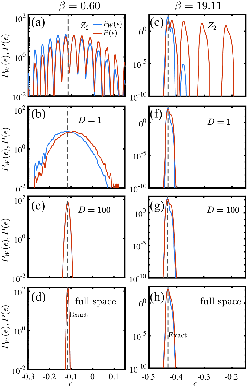
Figure 4: The probability distribution $P(\epsilon)$ and weighted $P_{W}(\epsilon)$ at high $\beta=0.60$ (left, a-d) and low temperature $\beta=19.11$ (right, e-h) obtained with different sample spaces: $Z_{2}$, $D=1$ [U(1)], $D=100$ and full sample space. In the calculations, we evolved the states $|{\Psi}\rangle$ including finite-$D$ MPS and vector.

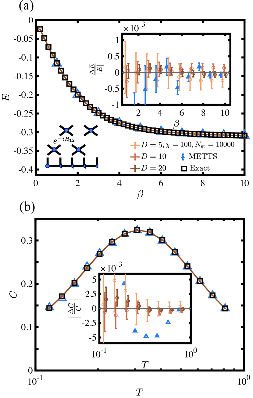
Figure 5: The results of energy and specific heat of the $L=50$ XY chain. (a) The energy results are well converged by retaining $\chi=100$ bond states and with $N_{\rm s}=10,000$ samples. Increasing bond dimension $D$ of the initial MPS can continuously improve the accuracy, as shown in the upper right inset of (a). The METTS results with $\chi=100$ and $N_{\rm s}=10,000$ are shown as a comparison. Left bottom inset illustrates the TEBD technique employed in the calculations. (b) The stoMPS results of specific heat show high accuracy when compared to the analytical solution, which are better than the METTS results shown in the inset. Reliable error bars for METTS results of specific heat is not available due to tricky issues in numerical differentiation.

To further analyze the sampling efficiency, we now move from sample space to energy space and estimate the unweighted and weighted probability density from Monto Carlo samplings

$$P(\epsilon)\simeq\frac{1}{N_{\rm s}}\sum_{n}K(\epsilon-\epsilon_{n};\sigma)$$ (3)

and

$$P_{W}(\epsilon)\simeq\frac{\sum_{n}\expectationvalue{e^{-\beta H}}{\psi_{n}}K(\epsilon-\epsilon_{n};\sigma)}{\sum_{n}\expectationvalue{e^{-\beta H}}{\psi_{n}}},$$ (4)

where $N_{\rm s}$ is the sample size, $\epsilon_{n}$ is the energy expectation value of the time-evolved sample $e^{-\beta H/2}|{\psi_{n}}\rangle$ and $K(\epsilon;\sigma)$ is a gaussian kernel. The weighted distribution density can be related with the energy expectation through (see Appendix D)

$$E=\int\epsilon P_{W}(\epsilon)d\epsilon.$$

In practice, we take $\sigma=2.5\times 10^{-3}$ and show the results with different sampling strategies in Fig. 4.

In Fig. 4(a-d), we present the results at relatively high temperature, where the probability distribution $P_{W}(\epsilon)$ becomes sharper and approaches the exact results as the bond dimension $D$ of the sampled MPS increases, indicating that the sampling efficiency is enhanced. Specifically, we find that by increasing the sampling space, the distribution $P_{W}(\epsilon)$ becomes more concentrated, as shown in Figs. 4(a-d). At low temperature, i.e., Fig. 4(e-h), the discrete $Z_{2}$ sampling scheme is far less efficient compared to the continuous $U(1)$ sampling scheme ($D=1$). This can be ascribed to the large number of low-weight samples in the $Z_{2}$-sampling strategy. When the total spin $\langle S^{z}_{\rm tot}\rangle$ of the initial state is nonzero, the overlap between the initial state and the ground state vanishes. As shown in Fig. 4(e), only about 33% of the samples have weights $W_{n}>10^{-4}$. As shown in Figs. 4(f-h), when we increase the initial bond dimension $D$ and thus more random parameters, the sample distribution becomes more concentrated, with the sample weight also increased.

III Applications on large-scale quantum lattice models

With the unbiased sampling schemes constructed, in the construction of Krylov subspace we need to carry out imaginary time evolution on the sampled initial MPS $|{\psi_{n}}\rangle$, i.e., $|{\beta_{n}}\rangle=e^{-\beta H/2}|{\psi_{n}}\rangle$. We randomly generate certain MPS with a bond dimension of $D$ and conduct imaginary-time evolution to obtain $|{\beta_{n}}\rangle$, with which the thermodynamic observables can be computed (c.f., Fig. 1). In the course of imaginary-time evolution, bond dimension of the MPS will increase and a truncation of geometric bond is thus required. Here we employ the time-evolving block decimation (TEBD) technique [47, 48] for MPS and retain maximally $\chi$ bond states in the calculations. Below, we present results of stoMPS applied to long 1D spin chains, as well as 2D square- and triangular-lattice Heisenberg models on cylinders of finite widths.

III.1 1D XY spin chain

Now we consider a more realistic but still exactly soluable problem, a $L=50$ XY chain, and showcase the powerfulness of stoMPS by calculating this model. To be specific, for the 1D Heisenberg chain $H=\sum_{i}h_{i,i+1}$, we exploit the TEBD technique to conduct the imaginary-time evolution on the MPS, which follows

$$e^{-\beta H}=(e^{-\tau H})^{N}=(e^{-\tau H_{\rm even}}e^{-\tau H_{\rm odd}})^{N}+{O}(\tau),$$ (5)

where $N\tau=\beta$, $H_{\rm even}=\sum_{i}h_{2i,2i+1}$ and $H_{\rm odd}=\sum_{i}h_{2i-1,2i}$. The stoMPS calculations are conducted with different bond dimensions $D$, all shared the same time evolution step length $\tau=0.05$, and with a maximal bond dimension $\chi=100$. The results are averaged over $N_{\rm s}=10,000$ samples to obtain well converged results.

In Fig. 5(a), we show the results of energy density and its relative errors with various initial $D$. The squares mark the analytical results of XY chain, and we find the stoMPS results, as well as METTS data, are in excellent agreement with the exact results. To see their relative errors, we show in the inset of Fig. 5(a) $\Delta E/|E|$, and find the accuracy gets continuously improved as $D$ increases. At high to intermediate temperatures, e.g.,$\beta\lesssim 5$, stoMPS with even small $D$ clearly outperform METTS; at sufficiently low temperature, e.g., $\beta=10$, the $D=20$ ($\chi=100$) stoMPS data have very similar accuracy as compared to the METTS results. With the same truncated bond dimension $\chi=100$ and sample number $N_{\rm s}=10,000$, in practice the METTS consumes 5 times CPU hours as compared to our stoMPS method, making latter superior performance in versatility, accuracy, and efficiency.

In Fig. 5(b), we present the specific heat results obtained using various methods. The black line represents the analytical solution, while the specific heat results computed by stoMPS were obtained through numerical differentiation. As shown in the figure, the results obtained by different methods are consistent with the analytical solution within the margin of error. The inset of Fig. 5(b) confirms that stoMPS has a clear advantage in computing the specific heat. stoMPS generates smoother data at different temperature points as it computes specific heat based on the same set of time-evolved MPSs, while METTS has to resample the procedure for each temperature point.

III.2 Square and triangular-lattice spin models

Beyond 1D system, we employ stoMPS method to simulate 2D Heisenberg antiferromagnetic lattice model wrapped on cylinder geometries. A conventional way to conduct such mapping is to follow the way routinely used in 2D density matrix renormalization group method. Here we showcase that the stoMPS can also be used to simulate the cylinders by “compressing” them into a 1D chain, as illustrated in the insets of Figs. 6(a,b). The corresponding MPS has a physical index with enlarged Hilbert space of dimension $d^{W}$, and the Hamiltonian only contains interactions between these nearest-neighboring composite sites. Thus, we can exploit TEBD techniques to simulate such systems similarly as in 1D chains, and compute the thermodynamics with high precision.

In Fig. 6(a), we present the results of the specific heat computed on a square lattice of size $4\times 8$ (cylinder width $W=4$ and length $L=8$), where the results are in good agreement with the recent tangent-space tensor renormalization group (tanTRG) approach, which is a state-of-the-art MPO-based method [30] for many-body systems. The specific heat curve displays a bell-like shape, with a maximum located at approximately $T/J\approx 0.6$, where $J=1$ is the spin exchange.

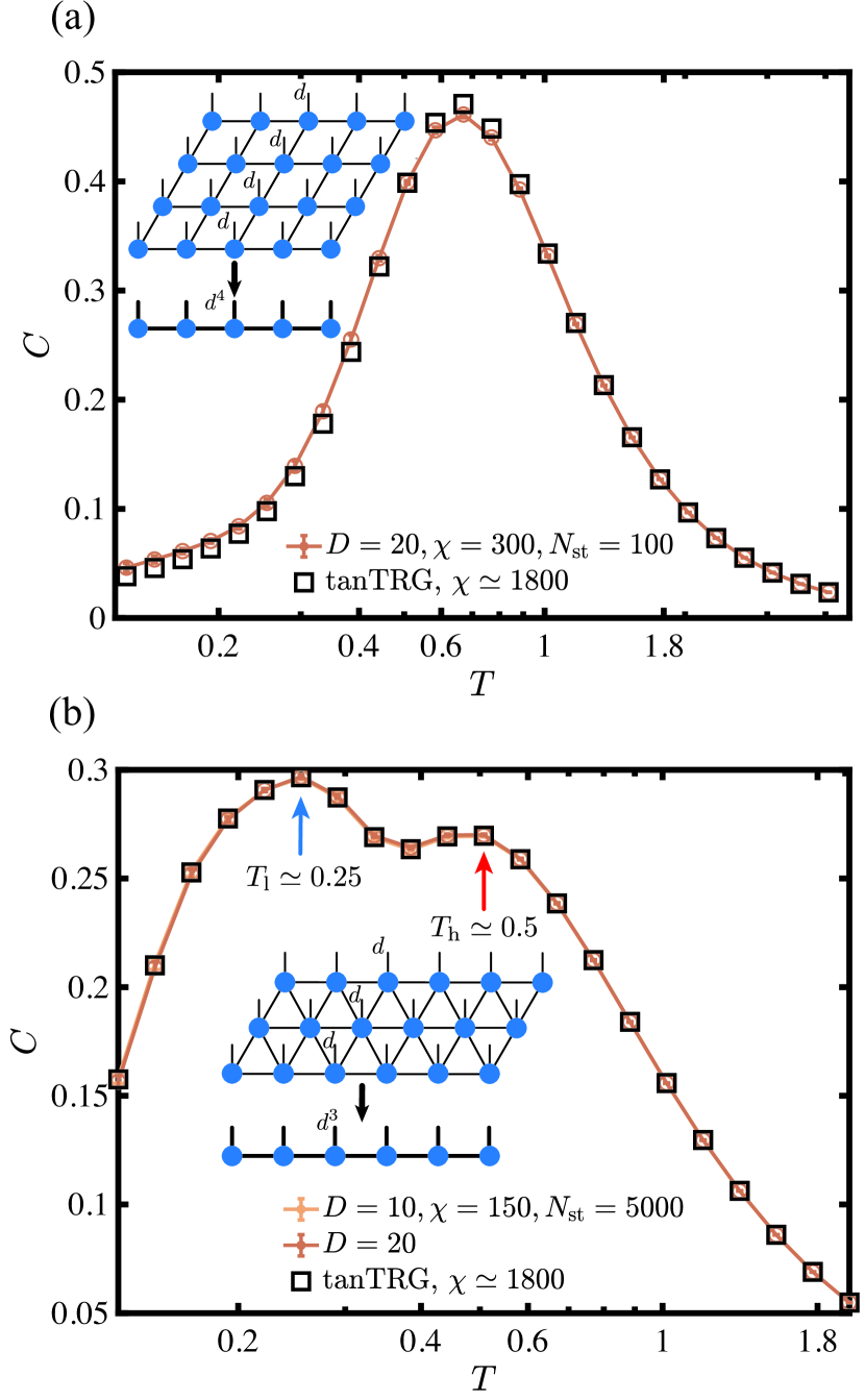
Figure 6: (a) Specific heat results of Heisenberg model on $4\times 8$ square lattice defined on cylinder geometry, and the stoMPS results with different $D$ are compared to that of tanTRG. (b) Results obtained on the $3\times 6$ triangular lattice, which exhibits double-peak structure in sharp contrast to that of the square-lattice Heisenberg model in (a).

In addition to the unfrustrated spin model, stoMPS can also be used to investigate frustrated quantum antiferromagnets. In Fig. 6(b), we present the specific heat results computed on a $3\times 6$ cylinder. Previous numerical studies of triangular lattice Heisenberg antiferromagnets have revealed the presence of two specific heat peaks at $T_{\rm h}/J\sim 0.5$ and $T_{\rm l}/J\sim 0.2$, respectively [28, 1], as also observed in experiments [49, 50]. It has been proposed that in the intermediate regime between the low-temperature scale $T_{\rm l}$ and the higher one $T_{\rm h}$, rotonlike excitations are activated with a strong chiral component and a significant contribution to the thermal entropy [51, 52]. These gapped roton excitations [53, 54], which bear a striking resemblance to the renowned roton thermodynamics in liquid helium, suppress the incipient $120^{\circ}$ order that emerges for temperatures below $T_{\rm l}$.

Here in Fig. 6(b), even on a width-3 cylinder such a double-peak specific heat curve can be clearly identified, and the results are well converged by retaining only $D=10,20$ bond states in the initialization and $\chi=150$ states during the imaginary-time evolution by TEBD. Our simulations on the square and triangular lattices show that the stoMPS method constitutes a practical approach for finite-temperature calculations of quantum lattice models, providing a valuable tool for studying frustrated quantum magnetism.

IV Summary and outlook

We construct an efficient algorithm for finite-temperature calculations by combining tensor networks and Monte Carlo sampling. From sampled MPS tensor $A$ with bond dimension $D$, we perform imaginary time evolution and then obtain very accurate results over sample average. We apply this method to spin chain and 2D spin systems including the Heisenberg model on the $4\times 8$ square and $3\times 6$ triangular lattices, and find the results are very accurate, where the sampling efficiency and accuracy can be improved by increasing the value of initial bond dimension $D$. Notably, we obtained two peaks of specific heat for the triangular lattice antiferromagnet. The algorithm has a number of advantages over the MPO-based algorithm, including good parallelism and high efficiency for low-temperature simulations, and has an overall superior performance than the existing MPS-based Monte Carlo method METTS.

Although stoMPS exhibits promising performance, there are still several points that require further improvements. For instance, stoMPS is not an importance sampling technique and may require enhancements to improve its sampling efficiency. Additionally, for sufficiently wide 2D lattice systems, the projected entangled-pair state (PEPS) method may outperform the MPS method. Our work provides a foundation for generalizing stochastic tensor networks from MPS to PEPS and may lead to even more accurate and efficient simulation methods for 2D quantum lattice models at finite temperature.

V Acknowledgement

This work was supported by the National Natural Science Foundation of China (Grant Nos. 12222412, 11974036, and 12047503), and the CAS Project for Young Scientists in Basic Research (YSBR-057). We thank the HPC-ITP for the technical support and generous allocation of CPU time.

Appendix A Finite-temperature Lanczos method

We briefly review the finite-temperature lanczos method (FTLM). Given a temperature $\beta=1/T$, the measurement of an operator $A$ reads

$$\langle A\rangle=\frac{1}{Z}{\rm Tr}[Ae^{-\beta H}]=\frac{1}{Z}\sum_{n}\langle n|Ae^{-\beta H}|n\rangle,$$ (6)

where $\{|n\rangle\}$ represent an orthonormal basis of the Hilbert space and $Z={\rm Tr}[e^{-\beta H}]$ is the partition function. Since the dimension of the Hilbert space increases exponentially as the system size increases, fully tracing becomes numerically impossible. On the other hand, with a given sample space, we have

$$\langle A\rangle=\overline{\langle A\rangle}:=\frac{\mathbb{E}\left[\expectationvalue{Ae^{-\beta H}}{\psi}\right]}{\mathbb{E}\left[\expectationvalue{e^{-\beta H}}{\psi}\right]},$$ (7)

if and only if

$$\mathbb{E}\left[|{\psi}\rangle\bra{\psi}\right]\propto I_{N},$$ (8)

with $I_{N}$ the identity operator in the N-dimension Hilbert space. Thus the measurement of $A$ can be obtained form a Monte Carlo sampling process

$$\langle A\rangle\simeq\frac{\sum_{n}^{N_{\rm s}}\langle\psi_{n}|e^{-\beta H}A|\psi_{n}\rangle}{\sum_{n}^{N_{\rm s}}\langle\psi_{n}|e^{-\beta H}|\psi_{n}\rangle},$$ (9)

where $N_{\rm s}$ is the sample size. In FTLM, the samples distribute uniformly on the unit sphere of the Hilbert space.

It remains to conduct the imaginary-time evolution of a given state using the Lanczos method, i.e.,

$$\begin{split}e^{-\beta H}&=\sum_{k}^{\infty}\frac{-\beta^{k}}{k!}H^{k}\\ &\simeq\sum_{k}^{\infty}\sum_{r}^{K}\frac{-\beta^{k}}{k!}\epsilon_{r}^{k}|\psi_{n}^{r}\rangle\langle\psi_{n}^{r}|\\ &=\sum_{r}^{K}e^{-\beta\epsilon_{r}}|\psi_{n}^{r}\rangle\langle\psi_{n}^{r}|,\end{split}$$ (10)

where $K$ represents the dimension of the Krylov subspace generated by $\{|\psi_{n}\rangle,H|\psi_{n}\rangle,...,H^{K-1}|\psi_{n}\rangle\}$ and $|\psi_{n}^{r}\rangle$ is the $r$-th eigenvector of $H$ with energy $\epsilon_{r}$ in the Krylov subspace.

The FTLM is a powerful tool that enables many-body calculations of the calculations of the finite-temperature and dynamic properties on finite-size systems. However, the vector representation of many-body state has a limitation as the computational cost grows exponentially with the system size. To extend the calculations to larger system sizes, a more efficient representation format such as the matrix product state (MPS) is required and developed in the present work.

Appendix B Lemma on random isometry

If $A\in{\rm St}(m\leq n,n)$ is a random isometry according to the Haar measure, then

$$\mathbb{E}\left[A^{\dagger}A\right]\propto I_{n\times n}.$$ (11)

Proof: Let $O\in{\rm O}(n)$ be any orthogonal matrix, then

$$O^{\dagger}\mathbb{E}\left[A^{\dagger}A\right]O=\mathbb{E}\left[O^{\dagger}A^{\dagger}AO\right]=\mathbb{E}\left[A^{\dagger}A\right]$$ (12)

since the Haar measure is invariant under the action of O($n$). The only matrix which permutes with the total O$(n)$ is the identity up to a coefficient, thus we have $\mathbb{E}\left[A^{\dagger}A\right]\propto I_{n\times n}$.

Appendix C Unitary MPO strategy

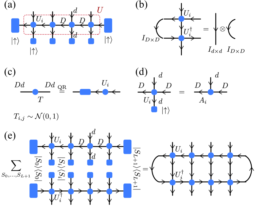
Figure 7: (a) Generating a random MPS from unitary MPO. (b) The canonical condition of random unitary MPO. (c) To sample the unitary matrix, we conduct a QR decomposition of the random matrix $T_{i,j}$ where each element is generated according to the standard normal distribution $\mathcal{N}(0,1)$. (d) The isometric tensor can be obtained form the unitary matrix with $|{\uparrow}\rangle:=(1,0,...,0)^{\rm T}$. (e) Tensor-network illustration of Eq. (13).

In this section, we will introduce an alternative method to obtain a random MPS satisfying Eq. (2). Note that the sample spaces of either $Z_{2}$ or U$(1)$ scheme introduced in the main text can be generated by a group of unitary operators acting on a trivial ferromagnetic (FM) state. Specifically, the $Z_{2}$ sampling corresponds to spin flipping ($\mathbb{Z}_{2}^{L}$), while the U$(1)$ sampling corresponds spin rotation $\prod_{1}^{L}$U(1). Based on this observation, we can construct a more general sample space by generalizing the unitary operation from local spin flip or rotation to a composite operation represented by a unitary matrix product operator (MPO) of finite bond dimension $D>1$, which applies to the FM state and generate a stochastic initial MPS [see Fig. 7(a)].

Here, we demonstrate that the random MPS $|{\psi}\rangle$ we obtain satisfies condition (2). To obtain the random isometric tensor, we proceed as follows. First, we generate a random $Dd\times Dd$ unitary matrix according to the Haar measure, as shown in Fig. 7(c,d). Then, we select the first $D$ rows of this matrix to construct an $D\times Dd$ isometric matrix. Additionally, we introduce two $D$-dimensional auxiliary states $|{\uparrow}\rangle$ and $|{\uparrow}\rangle$ at the boundaries to eliminate redundancy.

Note that a local spin-flip action on site $i$ (or boundary state) can be absorbed into the $U_{i}$ without changing the probability, i.e, $P(U|{\uparrow,\uparrow,...,\uparrow}\rangle\bra{\uparrow,\uparrow,...,\uparrow}U^{\dagger})=P(U|{\uparrow,\downarrow,...,\uparrow}\rangle\bra{\uparrow,\downarrow,...,\uparrow}U^{\dagger})$. As shown in Fig. 7(e), we have

$$\begin{split}&\mathbb{E}\left[U|{\uparrow,\uparrow,...,\uparrow}\rangle\bra{\uparrow,\uparrow,...,\uparrow}U^{\dagger}\right]\\ &=\frac{1}{D^{2}d^{L}}\sum_{s_{0},s_{1},...,s_{L+1}}\mathbb{E}\left[U|{S_{0},S_{1},...,S_{L+1}}\rangle\bra{S_{0},S_{1},...,S_{L+1}}U^{\dagger}\right]\\ &=\frac{1}{D^{2}d^{L}}\mathbb{E}\left[UU^{\dagger}\right].\end{split}$$ (13)

Note that $U_{i}$ is a unitary matrix, and we have $U_{i}U_{i}^{\dagger}=I$ [see Fig. 7(b)]. Recursively using the canonical condition, we arrive at $\mathbb{E}\left[U|{\uparrow,\uparrow,...,\uparrow}\rangle\bra{\uparrow,\uparrow,...,\uparrow}U^{\dagger}\right]=\frac{1}{Dd^{L}}I$.

Appendix D Probability density in energy space

Notice that the energy functional

$$E[\psi]:=\frac{\expectationvalue{e^{-\beta H}H}{\psi}}{\expectationvalue{e^{-\beta H}}{\psi}}$$ (14)

can be regarded as a random variable, which makes the energy space $\mathbb{R}$ a probability space with probability density

$$P(\epsilon):=\lim_{d\epsilon\rightarrow 0}\frac{\mathbb{P}(E\in[\epsilon,\epsilon+d\epsilon])}{d\epsilon}.$$ (15)

where $\mathbb{P}$ denotes the probability measure in sample space. $P(\epsilon)$ represents the energy distribution of the samples and thus can be used to characterize the energy typicality, i.e. if the obsevrved energy of sample states always has a high probability to be close to the average energy or not.

Note the average energy is not the expectation value corresponding to $P(\epsilon)$, instead, a Boltzmann weight $W[\psi]:=\expectationvalue{e^{-\beta H}}{\psi}$ is needed, i.e.

$$\begin{split}E(\beta)&=\frac{1}{Z(\beta)}\int E[\psi]W[\psi]\mathrm{d}\mathbb{P}\\ &=\frac{1}{Z(\beta)}\int d\epsilon\int\epsilon W[\psi]\frac{\mathrm{d}\mathbb{P}}{d\epsilon}\\ &:=\int\epsilon P_{W}(\epsilon)d\epsilon.\end{split}$$ (16)

Thus the weighted effective probability density reads

$$P_{W}(\epsilon)=\frac{1}{Z(\beta)}\lim_{d\epsilon\rightarrow 0}\int\limits_{S_{\epsilon}^{d\epsilon}}W[\psi]\frac{\mathrm{d}\mathbb{P}}{d\epsilon},$$ (17)

where $S_{\epsilon}^{d\epsilon}=\{|{\psi}\rangle|E[\psi]\in[\epsilon,\epsilon+d\epsilon]\}$ denotes the $[\epsilon,\epsilon+{\rm d}\epsilon]$ energy shell in sample space.

Both Eq. (15) and Eq. (17) can be estimated via standard kernel density estimation methods, resulting in Eq. (3) and Eq. (4) in the main text, respectively.

References

- Chen et al. [2019] L. Chen, D.-W. Qu, H. Li, B.-B. Chen, S.-S. Gong, J. von Delft, A. Weichselbaum, and W. Li, Two-temperature scales in the triangular-lattice heisenberg antiferromagnet, Phys. Rev. B 99, 140404 (2019).
- Li et al. [2020a] H. Li, Y. D. Liao, B.-B. Chen, X.-T. Zeng, X.-L. Sheng, Y. Qi, Z. Y. Meng, and W. Li, Kosterlitz-Thouless melting of magnetic order in the triangular quantum Ising material TmMgGaO4, Nat. Commun. 11, 1111 (2020a).
- Li et al. [2021] H. Li, H.-K. Zhang, J. Wang, H.-Q. Wu, Y. Gao, D.-W. Qu, Z.-X. Liu, S.-S. Gong, and W. Li, Identification of magnetic interactions and high-field quantum spin liquid in -RuCl3, Nat. Commun. 12, 4007 (2021).
- [4] Y. Gao, Y.-C. Fan, H. Li, F. Yang, X.-T. Zeng, X.-L. Sheng, R. Zhong, Y. Qi, Y. Wan, and W. Li, Spin supersolidity in nearly ideal easy-axis triangular quantum antiferromagnet Na2BaCo(PO4)2, npj Quantum Materials 7, 89.
- Yu et al. [2021] S. Yu, Y. Gao, B.-B. Chen, and W. Li, Learning the effective spin Hamiltonian of a quantum magnet, Chinese Physics Letters 38, 097502 (2021).
- Li et al. [2020b] H. Li, D.-W. Qu, H.-K. Zhang, Y.-Z. Jia, S.-S. Gong, Y. Qi, and W. Li, Universal thermodynamics in the kitaev fractional liquid, Phys. Rev. Research 2, 043015 (2020b).
- Jiménez et al. [2021] J. L. Jiménez, S. P. G. Crone, E. Fogh, M. E. Zayed, R. Lortz, E. Pomjakushina, K. Conder, A. M. Läuchli, L. Weber, S. Wessel, A. Honecker, B. Normand, C. Rüegg, P. Corboz, H. M. Rønnow, and F. Mila, A quantum magnetic analogue to the critical point of water, Nature 592, 370 (2021).
- Wang et al. [2023] J. Wang, H. Li, N. Xi, Y. Gao, Q.-B. Yan, W. Li, and G. Su, Plaquette singlet transition, magnetic barocaloric effect, and spin supersolidity in the shastry-sutherland model, Phys. Rev. Lett. 131, 116702 (2023).
- Wietek et al. [2021a] A. Wietek, Y.-Y. He, S. R. White, A. Georges, and E. M. Stoudenmire, Stripes, antiferromagnetism, and the pseudogap in the doped Hubbard model at finite temperature, Phys. Rev. X 11, 031007 (2021a).
- Lin et al. [2022] X. Lin, B.-B. Chen, W. Li, Z. Y. Meng, and T. Shi, Exciton proliferation and fate of the topological mott insulator in a twisted bilayer graphene lattice model, Phys. Rev. Lett. 128, 157201 (2022).
- Qu et al. [2022] D.-W. Qu, B.-B. Chen, X. Lu, Q. Li, Y. Qi, S.-S. Gong, W. Li, and G. Su, -wave Superconductivity, Pseudogap, and the Phase Diagram of -- Model at Finite Temperature (2022).
- Qu et al. [2023] X.-Z. Qu, D.-W. Qu, J. Chen, C. Wu, F. Yang, W. Li, and G. Su, Bilayer -- model and magnetically mediated pairing in the pressurized nickelate La3Ni2O7 (2023), arXiv:2307.16873 [cond-mat.str-el] .
- Mazurenko et al. [2017] A. Mazurenko, C. S. Chiu, G. Ji, M. F. Parsons, M. Kanász-Nagy, R. Schmidt, F. Grusdt, E. Demler, D. Greif, and M. Greiner, A cold-atom Fermi–Hubbard antiferromagnet, Nature 545, 462 (2017).
- Koepsell et al. [2021] J. Koepsell, D. Bourgund, P. Sompet, S. Hirthe, A. Bohrdt, Y. Wang, F. Grusdt, E. Demler, G. Salomon, C. Gross, and I. Bloch, Microscopic evolution of doped Mott insulators from polaronic metal to Fermi liquid, Science 374, 82 (2021).
- Chen et al. [2021] B.-B. Chen, C. Chen, Z. Chen, J. Cui, Y. Zhai, A. Weichselbaum, J. von Delft, Z. Y. Meng, and W. Li, Quantum many-body simulations of the two-dimensional Fermi-Hubbard model in ultracold optical lattices, Phys. Rev. B 103, L041107 (2021).
- Bursill et al. [1996] R. J. Bursill, T. Xiang, and G. A. Gehring, The density matrix renormalization group for a quantum spin chain at non-zero temperature, Journal of Physics: Condensed Matter 8, L583 (1996).
- Wang and Xiang [1997] X. Wang and T. Xiang, Transfer-matrix density-matrix renormalization-group theory for thermodynamics of one-dimensional quantum systems, Phys. Rev. B 56, 5061 (1997).
- Xiang [1998] T. Xiang, Thermodynamics of quantum heisenberg spin chains, Phys. Rev. B 58, 9142 (1998).
- Zwolak and Vidal [2004] M. Zwolak and G. Vidal, Mixed-state dynamics in one-dimensional quantum lattice systems: A time-dependent superoperator renormalization algorithm, Phys. Rev. Lett. 93, 207205 (2004).
- Feiguin and White [2005] A. E. Feiguin and S. R. White, Finite-temperature density matrix renormalization using an enlarged hilbert space, Phys. Rev. B 72, 220401 (2005).
- White [2009a] S. R. White, Minimally entangled typical quantum states at finite temperature, Phys. Rev. Lett. 102, 190601 (2009a).
- Stoudenmire and White [2010] E. M. Stoudenmire and S. R. White, Minimally entangled typical thermal state algorithms, New Journal of Physics 12, 055026 (2010).
- Li et al. [2011] W. Li, S.-J. Ran, S.-S. Gong, Y. Zhao, B. Xi, F. Ye, and G. Su, Linearized tensor renormalization group algorithm for the calculation of thermodynamic properties of quantum lattice models, Phys. Rev. Lett. 106, 127202 (2011).
- Czarnik et al. [2012] P. Czarnik, L. Cincio, and J. Dziarmaga, Projected entangled pair states at finite temperature: Imaginary time evolution with ancillas, Phys. Rev. B 86, 245101 (2012).
- Binder and Barthel [2015] M. Binder and T. Barthel, Minimally entangled typical thermal states versus matrix product purifications for the simulation of equilibrium states and time evolution, Phys. Rev. B 92, 125119 (2015).
- Dong et al. [2017] Y.-L. Dong, L. Chen, Y.-J. Liu, and W. Li, Bilayer linearized tensor renormalization group approach for thermal tensor networks, Phys. Rev. B 95, 144428 (2017).
- Chen et al. [2017] B.-B. Chen, Y.-J. Liu, Z. Chen, and W. Li, Series-expansion thermal tensor network approach for quantum lattice models, Phys. Rev. B 95, 161104 (2017).
- Chen et al. [2018] B.-B. Chen, L. Chen, Z. Chen, W. Li, and A. Weichselbaum, Exponential Thermal Tensor Network Approach for Quantum Lattice Models, Phys. Rev. X 8, 031082 (2018).
- Li et al. [2019] H. Li, B.-B. Chen, Z. Chen, J. von Delft, A. Weichselbaum, and W. Li, Thermal tensor renormalization group simulations of square-lattice quantum spin models, Phys. Rev. B 100, 045110 (2019).
- Li et al. [2023] Q. Li, Y. Gao, Y.-Y. He, Y. Qi, B.-B. Chen, and W. Li, Tangent Space Approach for Thermal Tensor Network Simulations of the 2D Hubbard Model, Phys. Rev. Lett. 130, 226502 (2023).
- White [2009b] S. R. White, Minimally entangled typical quantum states at finite temperature, Phys. Rev. Lett. 102, 190601 (2009b).
- Bruognolo et al. [2015] B. Bruognolo, J. Von Delft, and A. Weichselbaum, Symmetric minimally entangled typical thermal states, Phys. Rev. B 92, 115105 (2015).
- Goto and Danshita [2020] S. Goto and I. Danshita, Minimally entangled typical thermal states algorithm with trotter gates, Phys. Rev. Research 2, 043236 (2020).
- Wietek et al. [2021b] A. Wietek, R. Rossi, F. Šimkovic, M. Klett, P. Hansmann, M. Ferrero, E. M. Stoudenmire, T. SchÀfer, and A. Georges, Mott Insulating States with Competing Orders in the Triangular Lattice Hubbard Model, Physical Review X 11, 041013 (2021b).
- Fannes et al. [1992] M. Fannes, B. Nachtergaele, and R. F. Werner, Finitely correlated states on quantum spin chains, Communications in Mathematical Physics 144, 443 (1992).
- Klümper et al. [1993] A. Klümper, A. Schadschneider, and J. Zittartz, Matrix product ground states for one-dimensional spin-1 quantum antiferromagnets, Europhysics Letters (EPL) 24, 293 (1993).
- Jaklič and Prelovšek [1994] J. Jaklič and P. Prelovšek, Lanczos method for the calculation of finite-temperature quantities in correlated systems, Phys. Rev. B 49, 5065 (1994).
- Huang et al. [2018] R.-Z. Huang, H.-J. Liao, Z.-Y. Liu, H.-D. Xie, Z.-Y. Xie, H.-H. Zhao, J. Chen, and T. Xiang, A generalized lanczos method for systematic optimization of tensor network states, Chinese Phys. B 27, 070501 (2018), 1611.09574 .
- Schnack et al. [2020] J. Schnack, J. Richter, and R. Steinigeweg, Accuracy of the finite-temperature lanczos method compared to simple typicality-based estimates, Phys. Rev. Research 2, 013186 (2020).
- Garnerone et al. [2010] S. Garnerone, T. R. De Oliveira, and P. Zanardi, Typicality in random matrix product states, Phys. Rev. A 81, 032336 (2010).
- Sugiura and Shimizu [2012] S. Sugiura and A. Shimizu, Thermal pure quantum states at finite temperature, Phys. Rev. Lett. 108, 240401 (2012).
- Sugiura and Shimizu [2013] S. Sugiura and A. Shimizu, Canonical thermal pure quantum state, Phys. Rev. Lett. 111, 010401 (2013).
- Iwaki et al. [2021] A. Iwaki, A. Shimizu, and C. Hotta, Thermal pure quantum matrix product states recovering a volume law entanglement, Phys. Rev. Research 3, L022015 (2021).
- Note [1] More strictly speaking, the induced measure is a homogeneous space of O().
- Fasi and Robol [2021] M. Fasi and L. Robol, Sampling the eigenvalues of random orthogonal and unitary matrices, Linear Algebra and its Applications 620, 297 (2021).
- Birkhoff and Gulati [1979] G. Birkhoff and S. Gulati, Isotropic distributions of test matrices, Zeitschrift für angewandte Mathematik und Physik ZAMP 30, 148 (1979).
- Vidal [2004] G. Vidal, Efficient simulation of one-dimensional quantum many-body systems, Phys. Rev. Lett. 93, 040502 (2004).
- Daley et al. [2004] A. J. Daley, C. Kollath, U. Schollwöck, and G. Vidal, Time-dependent density-matrix renormalization-group using adaptive effective hilbert spaces, Journal of Statistical Mechanics: Theory and Experiment 2004, P04005 (2004).
- Rawl et al. [2017] R. Rawl, L. Ge, H. Agrawal, Y. Kamiya, C. R. Dela Cruz, N. P. Butch, X. F. Sun, M. Lee, E. S. Choi, J. Oitmaa, C. D. Batista, M. Mourigal, H. D. Zhou, and J. Ma, Ba3CoSb2O9: A spin- triangular-lattice Heisenberg antiferromagnet in the two-dimensional limit, Phys. Rev. B 95, 060412(R) (2017).
- Cui et al. [2018] Y. Cui, J. Dai, P. Zhou, P. S. Wang, T. R. Li, W. H. Song, J. C. Wang, L. Ma, Z. Zhang, S. Y. Li, G. M. Luke, B. Normand, T. Xiang, and W. Yu, Mermin-Wagner physics, phase diagram, and candidate quantum spin-liquid phase in the spin- triangular-lattice antiferromagnet , Phys. Rev. Materials 2, 044403 (2018).
- Elstner et al. [1993] N. Elstner, R. R. P. Singh, and A. P. Young, Finite temperature properties of the spin-1/2 Heisenberg antiferromagnet on the triangular lattice, Phys. Rev. Lett. 71, 1629 (1993).
- Elstner et al. [1994] N. Elstner, R. R. P. Singh, and A. P. Young, Spin-1/2 Heisenberg antiferromagnet on the square and triangular lattices: A comparison of finite temperature properties, J. Appl. Phys. 75, 5943 (1994).
- Zheng et al. [2005] W. Zheng, R. R. P. Singh, R. H. McKenzie, and R. Coldea, Temperature dependence of the magnetic susceptibility for triangular-lattice antiferromagnets with spatially anisotropic exchange constants, Phys. Rev. B 71, 134422 (2005).
- Zheng et al. [2006] W. Zheng, J. O. Fjærestad, R. R. P. Singh, R. H. McKenzie, and R. Coldea, Excitation spectra of the spin- triangular-lattice Heisenberg antiferromagnet, Phys. Rev. B 74, 224420 (2006).