capbtabboxtable[][\FBwidth]
Deep Dynamics: Vehicle Dynamics Modeling with a Physics-Informed Neural Network for Autonomous Racing
Abstract
Autonomous racing is a critical research area for autonomous driving, presenting significant challenges in vehicle dynamics modeling, such as balancing model precision and computational efficiency at high speeds (), where minor errors in modeling have severe consequences. Existing physics-based models for vehicle dynamics require elaborate testing setups and tuning, which are hard to implement, time-intensive, and cost-prohibitive. Conversely, purely data-driven approaches do not generalize well and cannot adequately ensure physical constraints on predictions. This paper introduces Deep Dynamics, a physics-informed neural network (PINN) for vehicle dynamics modeling of an autonomous racecar. It combines physics coefficient estimation and dynamical equations to accurately predict vehicle states at high speeds and includes a unique Physics Guard layer to ensure internal coefficient estimates remain within their nominal physical ranges. Open-loop and closed-loop performance assessments, using a physics-based simulator and full-scale autonomous Indy racecar data, highlight Deep Dynamics as a promising approach for modeling racecar vehicle dynamics.
I Introduction
As the field of autonomous vehicles has grown, the majority of research has been directed towards common driving situations. However, to enhance safety and performance, it is crucial to address the challenges presented by extreme driving environments. A quickly progressing area of research, autonomous racing, offers a valuable setting for this exploration. Recent advances in autonomous racing have been summarized comprehensively in [1]. Inspired by high-speed racing, competitions such as the Indy Autonomous Challenge [2], F1tenth [3], and Formula Driverless [4] have emerged where scaled and full-size driverless racecars compete to achieve the fastest lap times and overtake each other at speeds exceeding . The control software for autonomous racing must navigate racecars at extreme speeds and dynamic limits, a feat easily handled by skilled human racers but challenging for current low-speed optimized autonomous driving systems.
An essential aspect of autonomous racing is the precise modeling of a vehicle’s dynamic behavior. This encompasses using linearized or nonlinear differential equations to capture motion, tire dynamics, aerodynamics, suspension, steering, and drivetrain physics. While kinematic models focus on vehicle geometry, dynamic models delve deeper, estimating the acting forces to predict future movement, especially crucial in racing’s nonlinear regions characterized by rapid vehicle state changes and elevated dynamic loads. Obtaining precise coefficient values for modeling components like tires, suspension systems, and drivetrains is crucial, but extremely challenging. Determining tire coefficients (e.g. Pajecka coefficients[5]) involves extensive testing with specialized equipment (tire rigs) and significant time [6]. Additionally, calculating a racecar’s moment of inertia is a laborious task necessitating vehicle disassembly, precise component weighing and positioning, and the use of CAD software or multi-body physics simulations. Frequent recalculations are necessary to accommodate varying vehicle setups, track conditions, and tire wear, adding complexity to vehicle dynamics modeling, which is further complicated by the common omission of drivetrain dynamics, leading to incomplete models and suboptimal performance.
Deep neural networks (DNNs) have proven adept at capturing complex nonlinear dynamical effects [7], offering a simpler alternative to physics-based models as they obviate the need for extra testing equipment. Nevertheless, their substantial computational demands limit their integration for real-time model-predictive control (MPC), and they can often generate outputs unattainable by the actual system. Consequentially, this has sparked increasing interest in physics-informed neural networks (PINNs). For autonomous vehicles, an example of this approach is the Deep Pajecka Model [8]. However, this model has limitations such as reliance on sampling-based control, unconstrained Pacejka coefficient estimations, and not being tested on real data. We present Deep Dynamics, a PINN-based approach that to our best knowledge is the first model of its kind suited for vehicle dynamics modeling in autonomous racing - a domain distinctly marked by high accelerations and high speeds. This paper makes the following research contributions:
-
1.
We introduce Deep Dynamics - A PINN that can estimate the Pajecka tire coefficients, drivetrain coefficients, and moment of inertia that capture the complex and varying dynamics of an autonomous racecar.
-
2.
We introduce the Physics Guard layer designed to ensure that the model coefficients consistently remain within their physically meaningful ranges. This layer aligns the predictions of the PINN to adhere to the underlying physics governing vehicle dynamics.
-
3.
We examine both open-loop and closed-loop performance, utilizing a blend of simulation data and real-world data gathered from a full-scale autonomous racing car competing in the Indy Autonomous Challenge.
Our findings affirm that Deep Dynamics can effectively integrate with model-predictive control-based (MPC) trajectory following methods, all while leveraging the advantages of data-driven vehicle modeling without the complications associated with physics-based modeling.
II Related Work
Vehicle dynamics modeling is a thoroughly investigated subject for both passenger autonomous driving and autonomous racing. Physics-based vehicle dynamics models can vary greatly in complexity, ranging from simple point-mass to single-track (bicycle) models, to complex multi-body models [9]. Kinematic and dynamic single-track models are commonly used for vehicle dynamics modeling because they offer a good balance of simplicity and accuracy [10]. However, the accuracy of such models correlates with the accuracy of the model coefficients, which are often difficult to identify and tune [11]. Researchers have explored a variety of system identification approaches to learn the parameters of physics models through observations of the vehicle’s motion. [12] describes a method to estimate the coefficients for a vehicle’s drivetrain model and [13] focuses on identifying tire coefficients. Such methods often make a simplifying assumption that the model coefficients are time-invariant, which does not hold true in autonomous racing where coefficients may vary due to changes in racecar setups or tire wear throughout a race. Hybrid models that use a combination of data-driven and physics-based approaches have also been proposed. [14, 15, 16] use Gaussian Processes to correct the predictions of a simple physics model to match observed states. [17] addresses the same problem using a DNN. These approaches can capture time-variant dynamics but lack interpretability and provide no guarantees that corrected predictions will make physical sense.
Purely data-driven models, like in [18] and [19], learn vehicle dynamics using historical observations of the vehicle’s state and control inputs to train a DNN. [20] proposed the use of a recurrent neural network with a Gated Recurrent Unit (GRU) mechanism to accomplish the same task. These methods have shown the ability to perform well within the distribution of data they were trained on but, like as is the case with supervised machine learning approaches, they struggle to generalize on out-of-distribution data. The complexity and non-linearity of DNNs also limit the use of such models for model-based predictive control. Additionally, while purely data-driven models are great at learning complex non-linear patterns in the data, they are not designed to be consistent with the laws of physics and can produce state predictions that the vehicle cannot physically realize.
Recently, Physics-Informed Neural Networks (PINNs) for vehicle dynamics have been gaining traction as they adeptly merge the strengths of both physics-based and data-driven models. In the study by [21], PINNs were employed to model lateral dynamics in ships and quadrotors. Similarly, [22] trained a PINN to determine the dynamics of an unmanned surface vehicle. The closest related work to ours is the Deep Pacejka Model (DPM) introduced in [8], which estimates tire model coefficients for autonomous vehicles based on historical states and control inputs. However, as detailed in Section IV-A, the DPM bears inherent limitations that make it unsuitable for use in autonomous racing applications. Our research aims to address these limitations, introducing a new PINN model suitable for implementation in a real autonomous racecar.
III Problem Statement
| State Variable | Notation | State Equation |
|---|---|---|
| Horizontal Position () | = | |
| Vertical Position () | = | |
| Inertial Heading () | ||
| Longitudinal Velocity () | ||
| Lateral Velocity () | ||
| Yaw Rate () | ||
| Throttle (%) | ||
| Steering Angle () | ||
| Input Variable | Notation | |
| Throttle Change (%) | ||
| Steering Change () | ||
| Pacejka Tire Model | ||
| Drivetrain Model | ||
| Pacejka Coefficients | Drivetrain Coefficients | Vehicle Geometry |
| , , , , , | , , , | , , , |
We begin with a brief overview of vehicle dynamics followed by the problem formulation.
III-A Dynamic Single-Track Vehicle Model
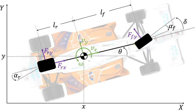
We model the autonomous racecar using a dynamic single-track vehicle model [10], with the state variables, discrete-time state equations, and notations listed in Table I. The accompanying free-body diagram for this model is shown in Figure 1. At time , the states of the system are , and the control inputs consist of changes to the vehicle’s throttle and steering i.e. . The single-track model (also known as the bicycle model) makes the assumption that the dynamics of the car can be described based on two virtual wheels located along the longitudinal axis of the racecar. A drivetrain model [14] estimates the longitudinal force at the rear wheels, , using drivetrain coefficients, and , the rolling resistance , and the drag coefficient . The Pacejka Magic Formula tire model [5] estimates the lateral tire forces on the front and rear wheels, and , inflicted by the vehicle’s movement and steering. The Pacejka model first calculates the sideslip angles for the front and rear wheels, and , using state and the distance between the vehicle’s center of gravity to the front and rear axles, and . The sideslip angles and sets of tire coefficients for the front and rear wheels, , are then used to estimate the lateral tire forces (Table I). Additional model coefficients include the mass, , and moment of inertia, , of the vehicle. The set of model coefficients together with the state and the control input fully describe the system’s dynamics.
Modeling Assumptions. We make the following modeling assumptions for the dynamic single-track model used in this work: 1. The model assumes that the racecar drives in 2D space despite the banking on real-world racetracks. The state equations can be modified to accommodate the banking angle of the racetrack. 2. We assume that there is no significant actuation delay for the control inputs , and . Actuation delays can be accounted for in the model, therefore this is just a simplifying assumption. 3. We assume that three of the model coefficients within are directly measurable and belong to the set of known coefficients, . These include the mass, , and geometric properties, and , which can be measured in a typical garage with corner weight scales. The remaining coefficients belong to the set of unknown coefficients, , because they are difficult to obtain without cost and time-intensive procedures. Therefore, , where and , , , , , , , , , , . Although the precise values of are unknown, we posit that each parameter is bounded within a known, physically meaningful nominal range, denoted as .
III-B Vehicle Dynamics Identification Problem
Consistent with the definitions in [8, 20], it is well established that the evolution of the model states can be completely described by the velocity states , , and . This can be seen in Table I, as the state equations for , , are fully dependent on the velocity terms. Hence, for the vehicle dynamics identification task, we exclusively utilize the state vector moving forward. Given a dataset , with state-input observations, we first split the data into two disjoint sets , where is used for model identification and is used for model verification. Our goal is to construct a predictive model that, given the current state , input , known coefficients , and estimated unknown coefficients , forecasts the subsequent state:
| (1) |
The unknown coefficients represent our current estimates of the unknown parameters . We know that can be realized through the state equations in Table I, therefore the accuracy of the model i.e. the mismatch between the model output and the observed from is governed by the precision of the unknown coefficient estimates . Given the nominal ranges for the unknown model coefficients , model , training data with samples, the formal problem can be stated as:
| (2) |
We approach the estimation of through a PINN that is intrinsically informed by the nominal ranges of .
IV Deep Dynamics
Physics-informed neural networks have emerged as an effective approach for modeling non-linear dynamic behaviors. The Deep Pacejka Model (DPM) [8] uses PINNs for autonomous driving, yet its limitations are pronounced when applied to the context of autonomous racing.
IV-A Limitations of the Deep Pacejka Model
The DPM uses a neural network to only estimate the Pacejka coefficients , and rather than using a physics-based drivetrain model, directly estimates the longitudinal force, , for an autonomous vehicle given a history of the vehicle’s state and control inputs. The DNN outputs are then used with the dynamic bicycle model state equations to predict the vehicle’s subsequent observed state, . Backpropagating results in a network that learns Pacejka coefficients and a purely data-driven drivetrain model that capture the vehicle’s dynamics.
The DPM suffers from several limitations. First, the DPM solves an unconstrained version of the problem in Equation 2, i.e. there are no bounds on . This can cause DPM to produce coefficients outside of the nominal ranges and , which could result in non-sensical predictions of the vehicle’s state. Second, the DPM assumes precise knowledge of the vehicle’s moment of inertia, . This is a very strong assumption because the precise value of requires knowledge of the weight distribution of the car. In addition, the DPM does not have a drivetrain model as there is no learned relation between the vehicle throttle, , and longitudinal wheel force, , which limits the DPM to using PID throttle control to track set by sampling-based MPC rather than directly controlling . More importantly, the Deep Pacejka Model was designed for low-speed autonomous driving and not for a high-speed racing environment.
IV-B Deep Dynamics
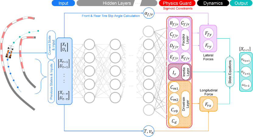
We propose the Deep Dynamics Model (DDM), a PINN capable of estimating the unknown coefficients for a single-track dynamical model (Section III-A) that are guaranteed to lie within their physically meaningful ranges, and . The model architecture for the DDM is shown in Figure 2. The DDM is given a history of length of vehicle states and control inputs, , which is then fed through the hidden layers of a DNN. We have introduced a Physics Guard layer which applies a Sigmoid activation function to the output, , of the last hidden layer and scales the result to produce between the bounds and using
| (3) |
A Sigmoid function was used for simplicity, but this mechanism could be implemented using any activation function with finite boundaries. The estimated coefficients and single-track model state equations are then used to predict , and the backpropagated loss function is computed using
| (4) |
across the state variables . The states and were not used in the loss function as the change in these states is determined by the control inputs and . In contrast to the DPM, the architecture of the DDM allows for longitudinal control using an MPC solver due to the inclusion of a physics-based drivetrain model. Additionally, the DDM does not assume prior knowledge of the vehicle’s moment of inertia, . Finally, the Physics Guard prevents the DDM from estimating non-sensical single-track model coefficients.
IV-C Model-Predictive Control with Deep Dynamics
For closed-loop testing, we use MPC to control the vehicle’s steering and throttle. An optimal raceline, , containing a sequence of reference points is tracked using MPC by solving for the optimal control inputs, , that minimize the cost function
| (5) |
across the forward prediction horizon . The first term, the tracking cost, penalizes deviations from the optimal raceline using the cost matrix . The second term, the actuation cost, penalizes rapid steering and throttle changes using the cost matrix . Once the optimal series of control inputs have been derived, the controller can enact and repeat this procedure.
At time , Deep Dynamics is used to predict the vehicle’s trajectory over the forward horizon, , by first estimating model coefficients using the observed states and control inputs from times to . These coefficients are held constant and used by MPC to propagate the predicted state of the vehicle from time to . Holding constant throughout allows an MPC solver to compute steering and throttle commands that minimize Equation 5 without having to differentiate through the DDM’s hidden layers, making it feasible to run in real-time.
V Experiments & Results
V-A Training and Testing Datasets
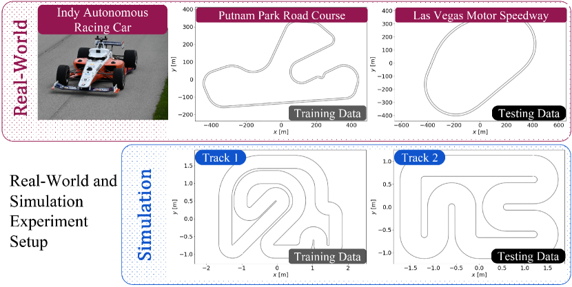
The open-loop performance of the Deep Dynamics Model and Deep Pacejka Model was evaluated on two both real and simulated data (shown in Figure 3). Real world data was compiled from a full-scale Indy autonomous racecar [23]. State information was sampled at a rate of 25 Hz from a 100 Hz Extended Kalman Filter which fuses measurements from two GNSS signals with RTK corrections and their IMU units. The training data, consisting of 13,418 samples was collected at the Putnam Park road course in Indianapolis, while the test set, , was curated from laps at the Las Vegas Motor Speedway and consists of 10,606 samples. Simulation dataset, , contains ground-truth vehicle state information from laps driven in a 1:43 scale racecar simulator [14], where the ground truth coefficient values are known. Data was collected from two different track configurations (Figure 3 Bottom) at 50 Hz using a pure-pursuit controller to drive the vehicle along a raceline. Track 1 was used to create the training dataset, and Track 2 was used to create the testing dataset, , with both consisting of 1,000 samples.
V-B Nominal Model Coefficient Ranges
The Physics Guard layer requires bounds and for each of the model coefficients estimated by Deep Dynamics. For the simulator, the ground truth is known and therefore, nominal ranges for the drivetrain coefficients and moment of inertia were created artificially by halving and doubling the ground-truth value for each coefficient. The ranges for Pacejka coefficients were set using the bounds described in [24]. For the real vehicle, the range for the moment of inertia, , was set to based on an estimate of provided by Dallara. The the drag coefficient, , and rolling resistance, , were given ranges from and , respectively, based on values estimated in [25]. The range for drivetrain coefficient was set to be based on the engine specification for Indy cars and the coefficient range for was set to to ensure force lost to engine friction would remain relatively small to the force generated.
V-C Evaluation Metrics
The root-mean-square error (RMSE) and maximum error () for the predicted longitudinal velocity, , lateral velocity, , and yaw rate, , were measured to compare each model’s one step prediction performance. In addition, we also generate horizon predictions using the estimated coefficients of each model and compute the average displacement error (ADE) and final displacement error (FDE) [26]. A time horizon of 300ms was used for generating trajectories on and a horizon of 600ms was used for .
V-D Open-Loop Testing
To highlight the inadequacy of presuming precise knowledge of the ground truth moment of inertia, , we trained three distinct iterations of the DPM: one given the ground truth value, termed DPM (GT); another with a value inflated by 20%, labeled DPM (+20%); and a third with a value reduced by 20%, referred to as DPM (-20%). The DPM (GT) offers a comparison against the best possible DPM while the others provide a comparison against models that are more realistic. While the choice of a deviation is arbitrary, it serves to emulate real-world scenarios where the exact value of the moment of inertia is unknown.
| Displacement (m) | |||||||||
|---|---|---|---|---|---|---|---|---|---|
| RMSE | RMSE | RMSE | ADE | FDE | |||||
| Sim Data | DPM (GT) | 0.0343 | 0.2017 | 0.1252 | 0.6762 | 4.306 | 30.606 | 0.0302 | 0.0942 |
| DPM (+20%) | 0.0270 | 0.2030 | 0.0889 | 0.5625 | 2.747 | 23.930 | 0.0263 | 0.0764 | |
| DPM (-20%) | 0.0331 | 0.2012 | 0.1202 | 0.6814 | 3.578 | 35.892 | 0.0467 | 0.1280 | |
| DDM (ours) | 1.506e-5 | 1.051e-4 | 1.839e-4 | 0.0013 | 0.0096 | 0.0549 | 3.77e-5 | 1.15e-4 | |
| Real Data | DPM (GT) | 0.0371 | 1.0390 | 0.1360 | 0.3123 | 0.0534 | 0.1795 | 0.2428 | 0.5644 |
| DPM (+20%) | 0.0339 | 1.0346 | 0.1306 | 0.3178 | 0.0322 | 0.0889 | 0.2400 | 0.5575 | |
| DPM (-20%) | 0.0347 | 1.0259 | 0.1342 | 0.3323 | 0.0471 | 0.1397 | 0.2384 | 0.5543 | |
| DDM (ours) | 0.0312 | 0.7976 | 0.0730 | 0.1837 | 0.0187 | 0.0788 | 0.1827 | 0.3840 | |
Table II shows the RMSE, , ADE, and FDE for the DDM and DPM variants on and . In simulation, our Deep Dynamics Model outperforms all variants of the DPM by over 4 orders of magnitude in terms of both RMSE and on and 2 orders of magnitude for and . On real data, DDM surpasses the DPM and its variants in terms of RMSE and by over for , for , and for in comparison to the best DPM. DDM’s ability to predict velocities with high accuracy translates into more precise future position predictions, as evidenced by its lowest ADE, and FDE across both simulated and real data. Even when given the ground-truth value of , the DPM still exhibited ADE and FDE nearly 2 orders of magnitude worse for both metrics. The highest performing DPM on the real data performed worse than the DDM as well, with 26% higher ADE and 36% higher FDE.
The models were also compared (shown in Table III) by examining their average Pacejka coefficient estimates to evaluate generalization and alignment with physics i.e. coefficients close to the true values indicate a model’s superior dynamic representation and predictive performance on new data. Known simulation coefficients provided a benchmark for the simulation data, while nominal coefficient ranges informed the assessment for the real data. The DPM’s estimated Pacejka coefficients for both simulation and real data diverged significantly from anticipated values, being either an order of magnitude different or contrary in sign. Conversely, the DDM produced estimates closely matching ground-truth values (highlighted in Table III) in simulation including accurately gauging the vehicle’s moment of inertia . Furthermore, the Physics Guard layer ensured that the coefficients derived from the generalize to different track conditions in .
| Sim Data | Actual | 5.579 | 1.200 | 0.192 | -0.083 | 5.385 | 1.269 | 0.173 | -0.019 | 2.78e-5 |
|---|---|---|---|---|---|---|---|---|---|---|
| DPM (GT) | -4.010 | -0.616 | 0.499 | 1.554 | -1.897 | -0.790 | 0.763 | 8.542 | NA | |
| DPM (+20%) | -1.455 | 0.654 | -0.646 | 2.335 | 1.283 | -0.792 | -0.763 | 5.920 | NA | |
| DPM (-20%) | -1.156 | 0.614 | -0.662 | 5.329 | -1.175 | 0.695 | -0.725 | 9.823 | NA | |
| DDM (ours) | 5.566 | 1.203 | 0.192 | -0.081 | 5.505 | 1.237 | 0.174 | -0.070 | 2.78e-5 | |
| Real Data | Range | 5-30 | 0.5-2 | 100-10000 | -2-0 | 5-30 | 0.5-2 | 100-10000 | -2-0 | 500-2000 |
| DPM (GT) | 12.845 | 12.356 | 2033.892 | 23.873 | 8.377 | 7.892 | -1327.340 | 4.291 | NA | |
| DPM (+20%) | 5.763 | -28.338 | -1249.052 | 27.035 | 0.095 | 9.587 | 863.780 | 12.189 | NA | |
| DPM (-20%) | 11.739 | 12.335 | 1109.978 | 49.836 | 4.823 | 3.056 | -703.947 | 28.165 | NA | |
| DDM (ours) | 6.630 | 1.047 | 3451.427 | -1.051 | 15.426 | 0.777 | 5335.260 | -0.733 | 1938.432 |
V-E Closed-Loop Testing
| Model | Lap Time (s) | Average Speed (m/s) | Track Violations |
|---|---|---|---|
| DPM (GT) | 6.16 | 1.721 | 2 |
| DPM (+20) | 6.00 | 1.732 | 3 |
| DPM (-20) | 5.94 | 1.728 | 3 |
| DDM (ours) | 5.38 | 2.010 | 0 |
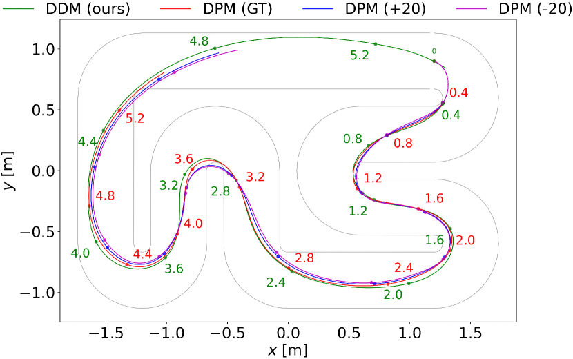
Closed-loop testing and comparison with DPM was performed using the MPC implementation described in Section IV-C. For DPM, a PID controller was used for throttle control (as opposed to a sampling-based MPC controller in the DPM paper). Figure 4 plots the time annotated traces for each model. Racing-relevant metrics such as lap time (s), average speed, and track boundary violations are reported in Table IV for a single lap with an initial of . DDM results in the fastest lap time of s while incurring boundary violations, and achieving the highest average speed of over (naively extrapolated to 311 as this is a 1:43 scale simulation). The inference time for DDM measured on a GeForce RTX 2080 Ti was approximately , making it suitable for real-time implementation.
V-F Hyperparameter Tuning
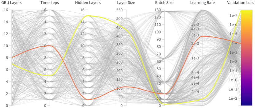
To ensure a fair comparison, rigorous hyperparameter tuning was conducted for both the DDM and DPM (shown in Figure 5). The learning rate, batch size, number of hidden layers, size of hidden layers, presence of and number of layers in the Gated Recurrent Unit (GRU), and the number of historical timesteps, , were all considered hyperparameters. Both models used the Mish activation function for the hidden layers and were optimized using Adam. Hyperparameters were tuned strategically using Optuna search. A validation set was created using 20% of the training set chosen randomly, and the DDM and DPM with the lowest validation loss were used to generate our results. This procedure was repeated for both real and simulation datasets.
VI Conclusion
We present Deep Dynamics, the first PINN vehicle dynamics model designed for use in autonomous racing. The network is capable of learning coefficients for a dynamic single-track vehicle model that accurately predicts the vehicle’s movement with little knowledge of the vehicle’s physical properties. The Physics Guard layer ensures that these coefficients remain in their physically meaningful range to guarantee the network obeys the laws of physics and improves generalization to unseen data. Our proposed work outperforms its predecessor in both open and closed-loop performance in a vehicle dynamics simulator and data collected from a real-world, full-scale autonomous racecar. Future work includes further closed-loop testing, starting with a high-fidelity racing simulator such as Autoverse, leading to implementing Deep Dynamics on a full-scale autonomous Indy racecar to demonstrate real-time performance and feasibility. In addition, in this work, the single-track model coefficients in the simulator were held constant, but we are also interested in further investigating the performance of the Deep Dynamics Model when these coefficients vary with time.
References
- [1] Johannes Betz et al. Autonomous vehicles on the edge: A survey on autonomous vehicle racing. IEEE Open Journal of Intelligent Transportation Systems, 3:458–488, 2022.
- [2] Alexander Wischnewski et al. Indy autonomous challenge – autonomous race cars at the handling limits, 2022.
- [3] Matthew O’Kelly et al. F1/10: An open-source autonomous cyber-physical platform. arXiv preprint arXiv:1901.08567, 2019.
- [4] Juraj Kabzan, Lukas Hewing, Alexander Liniger, and Melanie N Zeilinger. Learning-based model predictive control for autonomous racing. IEEE Robotics and Automation Letters, 4(4):3363–3370, 2019.
- [5] Hans B. Pacejka and Egbert Bakker. The magic formula tyre model. Vehicle System Dynamics, 21(sup001):1–18, 1992.
- [6] W. J. Langer and G. R. Potts. Development of a flat surface tire testing machine. SAE Transactions, 89:1111–1117, 1980.
- [7] Trent Weiss and Madhur Behl. Deepracing: A framework for autonomous racing. In 2020 Design, automation & test in Europe conference & exhibition (DATE), pages 1163–1168. IEEE, 2020.
- [8] Taekyung Kim, Hojin Lee, and Wonsuk Lee. Physics embedded neural network vehicle model and applications in risk-aware autonomous driving using latent features, 2022.
- [9] Matthias Althoff, Markus Koschi, and Stefanie Manzinger. Commonroad: Composable benchmarks for motion planning on roads. In 2017 IEEE Intelligent Vehicles Symposium (IV), pages 719–726, 2017.
- [10] Chang Mook Kang, Seung-Hi Lee, and Chung Choo Chung. Comparative evaluation of dynamic and kinematic vehicle models. In 53rd IEEE Conference on Decision and Control, pages 648–653, 2014.
- [11] Bernardo A. Hernandez Vicente, Sebastian S. James, and Sean R. Anderson. Linear system identification versus physical modeling of lateral–longitudinal vehicle dynamics. IEEE Transactions on Control Systems Technology, 29(3):1380–1387, 2021.
- [12] Jullierme Emiliano Alves Dias, Guilherme Augusto Silva Pereira, and Reinaldo Martinez Palhares. Longitudinal model identification and velocity control of an autonomous car. IEEE Transactions on Intelligent Transportation Systems, 16(2):776–786, 2015.
- [13] Chandrika Vyasarayani, Thomas Uchida, Ashwin Carvalho, and John McPhee. Parameter identification in dynamic systems using the homotopy optimization approach. Lecture Notes in Control and Information Sciences, 418:129–145, 01 2012.
- [14] Achin Jain, Matthew O’Kelly, Pratik Chaudhari, and Manfred Morari. BayesRace: Learning to race autonomously using prior experience. In Proceedings of the 4th Conference on Robot Learning (CoRL), 2020.
- [15] Juraj Kabzan, Lukas Hewing, Alexander Liniger, and Melanie N. Zeilinger. Learning-based model predictive control for autonomous racing. IEEE Robotics and Automation Letters, 4(4):3363–3370, 2019.
- [16] Jingyun Ning and Madhur Behl. Scalable deep kernel gaussian process for vehicle dynamics in autonomous racing. In 7th Annual Conference on Robot Learning, 2023.
- [17] Gabriel Costa, João Pinho, Miguel Ayala Botto, and Pedro U. Lima. Online learning of mpc for autonomous racing. Robotics and Autonomous Systems, 167:104469, 2023.
- [18] Nathan A. Spielberg et al. Neural network vehicle models for high-performance automated driving. Science Robotics, 4(28), 2019.
- [19] Grady Williams et al. Information theoretic mpc for model-based reinforcement learning. In 2017 IEEE International Conference on Robotics and Automation (ICRA), pages 1714–1721, 2017.
- [20] Leonhard Hermansdorfer, Rainer Trauth, Johannes Betz, and Markus Lienkamp. End-to-end neural network for vehicle dynamics modeling. In 2020 6th IEEE Congress on Information Science and Technology (CiSt), pages 407–412, 2020.
- [21] Alexandra Baier, Zeyd Boukhers, and Steffen Staab. Hybrid physics and deep learning model for interpretable vehicle state prediction. CoRR, abs/2103.06727, 2021.
- [22] Peng-Fei Xu et al. A physics-informed neural network for the prediction of unmanned surface vehicle dynamics. Journal of Marine Science and Engineering, 10(2), 2022.
- [23] Amar Kulkarni, John Chrosniak, et al. Racecar–the dataset for high-speed autonomous racing. arXiv:2306.03252, 2023.
- [24] Jose Luis Olazagoitia, Jesus Perez, and Francisco Badea Romero. Identification of tire model parameters with artificial neural networks. Applied Sciences, 10:9110, 12 2020.
- [25] B. Beckman. Physics of Racing Series. Stuttgart West, 1998.
- [26] Alexandre Alahi et al. Social lstm: Human trajectory prediction in crowded spaces. In 2016 IEEE Conference on Computer Vision and Pattern Recognition (CVPR), pages 961–971, 2016.