Investigating the Design Space of Diffusion Models for Speech Enhancement

Abstract

Diffusion models are a new class of generative models that have shown outstanding performance in image generation literature. As a consequence, studies have attempted to apply diffusion models to other tasks, such as speech enhancement. A popular approach in adapting diffusion models to speech enhancement consists in modelling a progressive transformation between the clean and noisy speech signals. However, one popular diffusion model framework previously laid in image generation literature did not account for such a transformation towards the system input, which prevents from relating the existing diffusion-based speech enhancement systems with the aforementioned diffusion model framework. To address this, we extend this framework to account for the progressive transformation between the clean and noisy speech signals. This allows us to apply recent developments from image generation literature, and to systematically investigate design aspects of diffusion models that remain largely unexplored for speech enhancement, such as the neural network preconditioning, the training loss weighting, the stochastic differential equation (SDE) , or the amount of stochasticity injected in the reverse process. We show that the performance of previous diffusion-based speech enhancement systems cannot be attributed to the progressive transformation between the clean and noisy speech signals. Moreover, we show that a proper choice of preconditioning, training loss weighting, SDE and sampler allows to outperform a popular diffusion-based speech enhancement system in terms of perceptual metrics while using fewer sampling steps, thus reducing the computational cost by a factor of four.

I Introduction

The presence of noise and reverberation in an acoustic scene can substantially reduce speech intelligibility, for both normal-hearing and hearing-impaired listeners [1, 2]. It can also reduce the performance of downstream tasks, such as automatic speech recognition (ASR)  [3] and speaker identification (SID)  [4]. Therefore, speech enhancement techniques that aim to restore speech intelligibility and quality by removing additive and convolutional distortions from noise and reverberation are crucial for a wide range of applications, such as telecommunications and hearing aid technology.

For the past years, the vast majority of studies on speech enhancement have favored deep neural network-based techniques, due to their superior performance over traditional statistical methods [5, 6, 7]. Deep neural network-based systems can be categorized into discriminative and generative models. Discriminative models learn a mapping from the input noisy speech to the output clean speech. They are trained in a supervised manner by presenting them with noisy and clean speech signals in pairs. On the other hand, generative models learn a probability distribution over clean speech. This probability distribution can be conditioned on an input noisy speech signal to perform speech enhancement. While discriminative models account for the vast majority of neural network-based speech enhancement systems [6], generative models represent an attractive approach, as learning the inherent properties of speech should enable robustness to arbitrary additive and convolutional distortions. Moreover, discriminative models have shown to produce unpleasant speech distortions that can be detrimental to downstream ASR tasks [8]. Generative approaches include generative adversarial networks (GANs)  [9], variational autoencoders (VAEs)  [10] and normalizing flows (NFs)  [11], which have all been applied to speech enhancement [12, 13, 14].

Diffusion models [15, 16, 17] have recently gained significant interest for the task of speech enhancement [18, 19, 20, 21, 22, 23, 24, 25]. As a new class of generative models, they have met great success in image generation [17, 26, 27], audio generation [28, 29, 30] and video generation [31, 32]. They consist in simulating a diffusion process by progressively adding Gaussian noise to the training data until it can be approximated as pure Gaussian noise. A neural network is then trained to undo this process and new samples can be generated by starting from new random noise realizations. In [18, 19], a discrete Markov chain formulation inspired by [17] was adopted, where the mean of the diffusion process was a linear interpolation between the clean and noisy speech signals. Speech enhancement was then performed by sampling from random noise centered around the noisy speech signal and solving the reverse diffusion process.

In [20, 21], a continuous SDE formulation inspired by [16] was proposed, where a novel drift term allowed for a progressive transformation of the mean of the diffusion process from the clean speech signal towards the noisy speech signal. Compared to the discrete Markov chain formulation in [18, 19], a continuous setting is more general and allows to use an arbitrary numerical solver to integrate the reverse process. It was also argued to allow for the derivation of an objective function that does not explicitly involve the difference between the clean speech signal and the noisy speech signal as opposed to [18, 19], thus making the training task purely generative. The introduced drift term was also argued to enable the system to perform the speech reconstruction task with environmental noises that are different from the stationary Gaussian noise used in the diffusion process [21].

Another common approach to diffusion-based speech enhancement consists in combining the diffusion model with a discriminative model that predicts a first estimate of the clean speech signal [33, 24, 25, 34]. The diffusion model is then tasked with removing unwanted distortions introduced by the discriminative model using e.g. denoising diffusion restoration models [35, 25], stochastic regeneration [33] or stochastic refinement [36, 34]. This approach avoids typical generative artifacts such as vocalizing and breathing effects, and considerably reduces the computational overhead from the diffusion model, since the number of steps in the reverse diffusion process can be reduced without losing performance [33]. Finally, another promising approach consists in using an unconditional diffusion model to solve inverse problems [35, 37, 38]. This was successfully applied to different audio applications such as music restoration [39], speech dereverberation [40] and source separation [41]. This approach paves the way for a new class of diffusion-based speech enhancement models that can be trained in an unsupervised way.

Despite these recent advances, several aspects of diffusion-based speech enhancement models remain poorly understood. In particular, the role of the drift term that pulls the mean of the diffusion process towards the noisy speech in [20, 21] is unclear. In our view, the noisy speech signal can be seen as a conditioner for the speech enhancement task in the same way as a text prompt in image generation, the only difference being that in speech enhancement, the conditioner has the same modality as the training data. Since such a drift is not needed to obtain good results in image generation, it is unclear why the success of diffusion-based speech enhancement should be attributed to it. Moreover, it was shown by Karras et al. [42] that multiple diffusion models that initially differed in their formulation can be framed in a common framework, allowing to better compare them. However, due to the nature of the drift term used for speech enhancement in [20, 21], the resulting diffusion model cannot be directly included in the framework from [42]. As a consequence, it is difficult to translate recent advances from image generation literature to speech enhancement. Finally, while some design aspects of diffusion-based speech enhancement were analyzed in subsequent works [43, 44], many remain unexplored, such as the neural network preconditioning [42], the loss weighting, the SDE , or the amount of stochasticity injected when integrating the reverse process.

Our contributions in this work are as follows:

• We extend a diffusion model framework previously laid in image generation literature [42] to include a recently proposed diffusion-based speech enhancement system [20, 21] where the long-term mean of the diffusion process is non-zero and equal to the conditioner. Compared to [45] where we used a change of variable to consider the SDE satisfied by the environmental noise and fit in the framework laid in [42], we instead propose here a more general approach that models the clean speech signal and accounts for an eventual drift of the diffusion process.

• Using this new framework, we show that the success of diffusion-based speech enhancement models cannot be attributed to the addition of a drift term that pulls the mean of the diffusion process towards the conditioner. This also proves that a mismatch between the final distribution of the forward process and the prior distribution used to initialize the reverse process is not necessarily responsible for a drop in performance as suggested in [44].

• We systematically investigate the design space of diffusion models for speech enhancement by experimenting with different neural network preconditionings [42], loss weightings, SDEs , and amounts of stochasticity injected when integrating the reverse process.

• This investigation results in a system that outperforms a popular diffusion-based baseline in terms of perceptual metrics while using fewer sampling steps, thus allowing for a fourfold decrease in computational cost.

In Sect. II, we go over some related work on diffusion models and their adaptation to speech enhancement. In Sect. III, we prove how the framework from [42] can be extended to include the diffusion-based speech enhancement models from [20, 21]. In Sect. IV, we describe the experimental setup. Finally in Sect. V, we present and discuss the results.

II Related work

II-A Diffusion models

A diffusion model progressively transforms clean training data ${\boldsymbol{x}_{0}\mskip-1.5mu\in\mskip-1.5mu\mathbb{R}^{d}}$ with distribution ${p_{\mathrm{data}}}$ into isotropic Gaussian noise. This transformation can be modeled as a diffusion process ${\boldsymbol{x}_{t}\mskip-1.5mu\in\mskip-1.5mu\mathbb{R}^{d}}$ indexed by a continuous variable ${t\mskip-1.5mu\in\mskip-1.5mu[0,\mskip-1.5mu1]}$ satisfying the following general SDE ,

$$\mathop{}\!\mathrm{d}\boldsymbol{x}_{t}=\boldsymbol{f}(t,\boldsymbol{x}_{t})\mathop{}\!\mathrm{d}t+g(t)\mathop{}\!\mathrm{d}\boldsymbol{\omega}_{t},$$ (1)

where ${\boldsymbol{f}(t,\cdot):\mathbb{R}^{d}\mapsto\mathbb{R}^{d}}$ is the drift coefficient, ${g:\mathbb{R}\mapsto\mathbb{R}^{+}}$ is the diffusion coefficient and ${\boldsymbol{\omega}_{t}\mskip-1.5mu\in\mskip-1.5mu\mathbb{R}^{d}}$ is a standard Wiener process. The goal of a diffusion model is to solve the associated reverse-time SDE  [46], such that new samples can be generated starting from random Gaussian noise realizations at ${t\!=\!1}$. The reverse-time SDE associated with Eq. (1) is

$$\mathop{}\!\mathrm{d}\boldsymbol{x}_{t}=\left[\boldsymbol{f}(t,\boldsymbol{x}_{t})-g^{2}\mskip-0.75mu(t)\nabla_{\boldsymbol{x}_{t}}\!\log p_{t}(\boldsymbol{x}_{t})\right]\mathop{}\!\mathrm{d}t+g(t)\mathop{}\!\mathrm{d}\boldsymbol{\omega}_{t},$$ (2)

where ${\nabla_{\boldsymbol{x}_{t}}\!\log p_{t}(\boldsymbol{x}_{t})}$ is termed the score function, which is intractable as it involves marginalizing over the unknown distribution of the training data ${p_{\mathrm{data}}}$,

$$p_{t}(\boldsymbol{x}_{t})=\int_{\mathbb{R}^{d}}p_{0t}(\boldsymbol{x}_{t}|\boldsymbol{x}_{0})p_{\mathrm{data}}(\boldsymbol{x}_{0})\mathop{}\!\mathrm{d}\boldsymbol{x}_{0},$$ (3)

where the conditional probability density function (PDF) ${p_{0t}}$ is commonly referred to as the perturbation kernel. Even though ${\nabla_{\boldsymbol{x}_{t}}\!\log p_{t}(\boldsymbol{x}_{t})}$ is intractable, a neural network can be trained to approximate it via score matching [47, 48, 49],

$$\boldsymbol{s}_{\boldsymbol{\theta}}(\boldsymbol{x}_{t},t)\simeq\nabla_{\boldsymbol{x}_{t}}\!\log p_{t}(\boldsymbol{x}_{t}),$$ (4)

where ${\boldsymbol{s}_{\boldsymbol{\theta}}}$ is the score model. New samples can then be generated from random Gaussian noise realizations by substituting ${\nabla_{\boldsymbol{x}_{t}}\!\log p_{t}(\boldsymbol{x}_{t})}$ with ${\boldsymbol{s}_{\boldsymbol{\theta}}(\boldsymbol{x}_{t},t)}$ in Eq. (2) and integrating Eq. (2) using an arbitrary numerical solver (e.g. Euler-Maruyama or Runge-Kutta methods). The number of sampling steps ${n_{\mathrm{steps}}}$ used to discretize the time axis and integrate the reverse process controls the number of neural network evaluations. Therefore, ${n_{\mathrm{steps}}}$ defines a compromise between sample quality and computational cost.

The drift coefficient is commonly chosen to have the form ${\boldsymbol{f}(t,\boldsymbol{x}_{t})\!=\!f(t)\mskip 1.5mu\boldsymbol{x}_{t}}$, such that the SDE in Eq. (1) becomes

$$\mathop{}\!\mathrm{d}\boldsymbol{x}_{t}=f(t)\mskip 1.5mu\boldsymbol{x}_{t}\mathop{}\!\mathrm{d}t+g(t)\mathop{}\!\mathrm{d}\boldsymbol{\omega}_{t}.$$ (5)

The perturbation kernel of this SDE turns out to be Gaussian and can be calculated using Eqs. (5.50) and (5.51) in [50],

$$p_{0t}(\boldsymbol{x}_{t}|\boldsymbol{x}_{0})=\mathcal{N}\big{(}\boldsymbol{x}_{t};s(t)\mskip 1.5mu\boldsymbol{x}_{0},\sigma^{2}\mskip-0.75mu(t)\mskip 1.5mu\mathbf{I}\big{)},$$ (6)

where

and ${\mathcal{N}(\,\cdot\,;\boldsymbol{\mu},\boldsymbol{\Sigma})}$ denotes a multivariate Gaussian PDF with mean ${\boldsymbol{\mu}\mskip-1.5mu\in\mskip-1.5mu\mathbb{R}^{d}}$ and covariance matrix ${\boldsymbol{\Sigma}\mskip-1.5mu\in\mskip-1.5mu\mathbb{R}^{d\times d}}$. This allows to directly sample ${\boldsymbol{x}_{t}}$ during training for any ${t}$ without having to numerically solve the forward SDE in Eq. (5). However, during inference, since ${\boldsymbol{x}_{0}}$ is unknown, noise cannot be sampled around ${s(t)\mskip 1.5mu\boldsymbol{x}_{0}}$ to initialize the reverse process at ${t\!=\!1}$, unless ${s(1)\!=\!0}$. In practice, it is common to use the zero-mean prior distribution ${\mathcal{N}\big{(}\mskip 1.5mu\cdot\,;\mathbf{0},\sigma^{2}\mskip-0.75mu(1)\mskip 1.5mu\mathbf{I}\big{)}}$, even if this does not match ${p_{01}}$.

II-B Common SDEs

The joint parametrization of ${f(t)}$, ${g(t)}$, ${s(t)}$ and ${\sigma(t)}$ is commonly referred to as the noise schedule. One can first fix ${f(t)}$ and ${g(t)}$ and derive the corresponding ${s(t)}$ and ${\sigma(t)}$ from Eq. (7), or alternatively one can first fix ${s(t)}$ and ${\sigma(t)}$ and derive the corresponding ${f(t)}$ and ${g(t)}$ after reverting Eq. (7),

$$f(t)=\frac{\mathop{}\!\mathrm{d}}{\mathop{}\!\mathrm{d}t}\Big{[}\log s(t)\Big{]}\quad\text{and}\quad g(t)=s(t)\sqrt{\frac{\mathop{}\!\mathrm{d}}{\mathop{}\!\mathrm{d}t}\left[\frac{\sigma^{2}\mskip-0.75mu(t)}{s^{2}\mskip-0.75mu(t)}\right]}.$$ (8)

Recent studies [51, 52, 53, 54] argued that the noise schedule should be defined in terms of the log of the signal-to-noise ratio (SNR) of the diffusion process ${\lambda(t)}$,

$$\lambda(t)=\log\frac{s^{2}\mskip-0.75mu(t)}{\sigma^{2}\mskip-0.75mu(t)}.$$ (9)

Common choices for the drift and diffusion coefficients can be categorized into the variance exploding (VE) and variance preserving (VP) assumptions [16].

II-B1 VE assumption

The VE assumption consists in setting ${f(t)\!=\!0}$, which leads to

$$s(t)=1\quad\text{and}\quad g(t)=\sqrt{\frac{\mathop{}\!\mathrm{d}}{\mathop{}\!\mathrm{d}t}\Big{[}\sigma^{2}\mskip-0.75mu(t)\Big{]}}.$$ (10)

Song et al. [16] proposed the following noise schedule,

$$\sigma^{2}\mskip-0.75mu(t)=\sigma_{\mathrm{min}}^{2}\left[\left(\frac{\sigma_{\mathrm{max}}}{\sigma_{\mathrm{min}}}\right)^{2t}-1\right],$$ (11)

where ${\sigma_{\mathrm{min}},\sigma_{\mathrm{max}}\mskip-1.5mu\in\mskip-1.5mu\mathbb{R}^{+},\sigma_{\mathrm{min}}\!<\!\sigma_{\mathrm{max}}}$ are two hyperparameters. As a consequence,

$$g(t)=\sigma_{\mathrm{min}}\left(\frac{\sigma_{\mathrm{max}}}{\sigma_{\mathrm{min}}}\right)^{t}\sqrt{2\log\frac{\sigma_{\mathrm{max}}}{\sigma_{\mathrm{min}}}}.$$ (12)

II-B2 VP assumption

The VP assumption consists in fixing ${s^{2}\mskip-0.75mu(t)\!+\!\sigma^{2}\mskip-0.75mu(t)\!=\!1}$, which leads to

$$f(t)=-\frac{1}{2}\beta(t)\quad\text{and}\quad g(t)=\sqrt{\beta(t)},$$ (13)

where ${\beta:[0,\mskip-1.5mu1]\mapsto\mathbb{R}^{+}}$ is a hyperparameter. Song et al. [16] proposed a linear noise schedule of the following form,

$$\beta(t)=\beta_{\mathrm{min}}+t\,(\beta_{\mathrm{max}}-\beta_{\mathrm{min}}),$$ (14)

where ${\beta_{\mathrm{min}},\beta_{\mathrm{max}}\mskip-1.5mu\in\mskip-1.5mu\mathbb{R}^{+},\beta_{\mathrm{min}}\!<\!\beta_{\mathrm{max}}}$. The perturbation kernel can then be derived using

$$s(t)=e^{-\frac{1}{2}\int_{0}^{t}\beta(\xi)\mathop{}\!\mathrm{d}\xi}\quad\text{and}\quad\sigma^{2}\mskip-0.75mu(t)=1-e^{-\int_{0}^{t}\beta(\xi)\mathop{}\!\mathrm{d}\xi}.$$ (15)

Another common setting under the VP assumption is the family of cosine schedule [55, 53],

$$\lambda(t)=-2\log\left(\tan\frac{\pi t}{2}\right)+2\nu,$$ (16)

where ${\nu}$ is a parameter controlling the center of the log-SNR distribution. The derivations of the perturbation kernel parameters ${s(t)}$ and ${g(t)}$ and the SDE coefficients ${f(t)}$ and ${g(t)}$ from ${\lambda(t)}$ are detailed in Appendix A.

II-C Elucidating the Design Space of Diffusion-Based Generative Models (EDM)

Karras et al. [42] showed that previous diffusion model formulations can be framed in a common framework denoted here as EDM. More specifically, they showed that

• The general SDE in Eq. (5) is equivalent to a simpler, unscaled SDE satisfied by the unscaled process ${\bar{\boldsymbol{x}}_{t}\!=\!\frac{\boldsymbol{x}_{t}}{s(t)}}$,

  $$\mathop{}\!\mathrm{d}\bar{\boldsymbol{x}}_{t}=\frac{g(t)}{s(t)}\mathop{}\!\mathrm{d}\boldsymbol{\omega}_{t}.$$ (17)

  The perturbation kernel of the unscaled process is

  $$\bar{p}_{0t}(\bar{\boldsymbol{x}}_{t}|\boldsymbol{x}_{0})=\mathcal{N}\big{(}\bar{\boldsymbol{x}}_{t};\boldsymbol{x}_{0},\bar{\sigma}(t)^{2}\mskip-0.75mu(\mskip 1.5mu)\mathbf{I}\big{)},$$ (18)

  where

  $$\bar{\sigma}^{2}\mskip-0.75mu(t)=\frac{\sigma^{2}\mskip-0.75mu(t)}{s^{2}\mskip-0.75mu(t)}=\int_{0}^{t}\frac{g^{2}\mskip-0.75mu(\xi)}{s^{2}\mskip-0.75mu(\xi)}\mathop{}\!\mathrm{d}\xi.$$ (19)

  Karras et al. [42] suggested using ${s(t)\!=\!1}$. This is intuitive since the network is conditioned on the state index ${t}$ and can thus learn to undo the deterministic scaling ${s(t)}$ before denoising. This is in line with studies defining the noise schedule in terms of the log-SNR ${\lambda(t)}$ [51, 52, 53, 54], as ${\bar{\sigma}^{2}\mskip-0.75mu(t)\!=\!e^{-\lambda(t)}}$. The perturbation kernel of the scaled process ${\boldsymbol{x}_{t}\!=\!s(t)\mskip 1.5mu\bar{\boldsymbol{x}}_{t}}$ can be rewritten as

  $$p_{0t}(\boldsymbol{x}_{t}|\boldsymbol{x}_{0})=\mathcal{N}\big{(}\boldsymbol{x}_{t};s(t)\mskip 1.5mu\boldsymbol{x}_{0},s^{2}\mskip-0.75mu(t)\bar{\sigma}^{2}\mskip-0.75mu(t)\mskip 1.5mu\mathbf{I}\big{)}.$$ (20)

• The marginal distribution ${p_{t}}$ can be written as

  $$p_{t}(\boldsymbol{x}_{t})=s(t)^{-d}\bar{p}(\bar{\boldsymbol{x}}_{t},\bar{\sigma}(t)),$$ (21)

  where ${\bar{p}}$ is a mollified version of ${p_{\mathrm{data}}}$ obtained by adding i.i.d. Gaussian noise to the samples,

  $$\bar{p}(\cdot,\sigma)=p_{\mathrm{data}}\ast\mathcal{N}(\mathbf{0},\sigma^{2}\mskip 1.5mu\mathbf{I}),$$ (22)

  where ${\ast}$ is the convolution operator between PDFs . As a consequence, the score function can be rewritten as

  $$\nabla_{\boldsymbol{x}_{t}}\!\log p_{t}(\boldsymbol{x}_{t})=\nabla_{\boldsymbol{x}_{t}}\!\log\bar{p}(\bar{\boldsymbol{x}}_{t},\bar{\sigma}(t)),$$ (23)

  which means that it can be evaluated on the unscaled process ${\bar{\boldsymbol{x}}_{t}}$. Let ${\boldsymbol{D}}$ denote the optimal denoiser that minimizes a weighted ${\mathcal{L}_{2}}$-loss between the clean training data ${\boldsymbol{x}_{0}}$ and the output from the unscaled diffused data ${\bar{\boldsymbol{x}}_{t}}$,

  $$\mathbb{E}_{\boldsymbol{x}_{0}}\mathbb{E}_{t,\bar{\boldsymbol{x}}_{t}|\boldsymbol{x}_{0}}\Big{[}w(t)\left\|\boldsymbol{D}(\bar{\boldsymbol{x}}_{t},t)-\boldsymbol{x}_{0}\right\|_{2}^{2}\Big{]},$$ (24)

  where ${w:[0,\mskip-1.5mu1]\mapsto\mathbb{R}^{+}}$ is the loss weighting function. Karras et al. [42] showed that the score function can be expressed as a function of the optimal denoiser ${\boldsymbol{D}}$,

  $$\nabla_{\boldsymbol{x}_{t}}\!\log\bar{p}(\bar{\boldsymbol{x}}_{t},\bar{\sigma}(t))=\frac{\boldsymbol{D}(\bar{\boldsymbol{x}}_{t},t)-\bar{\boldsymbol{x}}_{t}}{s(t)\bar{\sigma}^{2}\mskip-0.75mu(t)}.$$ (25)

• The fitted denoiser ${\boldsymbol{D}_{\boldsymbol{\theta}}}$ trained to minimize Eq. (24) can be expressed as a function of the raw neural network layers ${\boldsymbol{F}_{\boldsymbol{\theta}}}$. Such parametrization is referred to as preconditioning and has the form

  Karras et al. [42] suggested the following parametrization for ${c_{\mathrm{skip}}}$, ${c_{\mathrm{out}}}$, ${c_{\mathrm{in}}}$, ${c_{\mathrm{noise}}}$ and ${w}$ based on first principles (effective input unit variance, effective target unit variance and uniform effective loss weight),

  where ${\sigma_{\mathrm{data}}^{2}}$ is the variance of the data distribution ${p_{\mathrm{data}}}$.

II-D Score-based Generative Model for Speech Enhancement (SGMSE)

Welker et al. [20] and Richter et al. [21] adapted the diffusion model from Song et al. [16] to perform speech enhancement by conditioning the clean speech generation process on the noisy speech signal. They considered complex-valued short-time Fourier transform (STFT) representations of the signals flattened into ${d\!=\!KT}$-dimensional vectors, where ${K}$ is the number of frequency bins and ${T}$ is the number of frames. They trained the score model using pairs of clean and noisy speech signals ${\boldsymbol{x}_{0},\boldsymbol{y}\mskip-1.5mu\in\mskip-1.5mu\mathbb{C}^{d}}$ in a supervised manner such that

$$\boldsymbol{s}_{\boldsymbol{\theta}}(\boldsymbol{x}_{t},\boldsymbol{y},t)\simeq\nabla_{\boldsymbol{x}_{t}}\!\log p_{t}(\boldsymbol{x}_{t}|\boldsymbol{y}).$$ (28)

They defined their diffusion equation as

that is ${\boldsymbol{f}(t,\boldsymbol{x}_{t})\!=\!-\gamma(\boldsymbol{x}_{t}\!-\!\boldsymbol{y})}$ where ${\gamma}$ is a hyperparameter denoted as the stiffness, and ${g(t)}$ is the same as the VE SDE from [16] and shown in Eq. (12). This SDE was inspired by the Ornstein-Uhlenbeck (OU) SDE  [56] and results in an exponential decay of the mean of the diffusion process from ${\boldsymbol{x}_{0}}$ towards ${\boldsymbol{y}}$. We refer to this SDE as the OUVE SDE .

The drift coefficient ${\boldsymbol{f}(t,\boldsymbol{x}_{t})\!=\!-\gamma(\boldsymbol{x}_{t}\!-\!\boldsymbol{y})}$ in Eq. (29) cannot be written in the form ${f(t)\mskip 1.5mu\boldsymbol{x}_{t}}$, which means that the perturbation kernel cannot be calculated using Eqs. (6) and (7). Moreover, the model cannot be framed in the EDM framework, since we cannot find a scaling factor ${s(t)}$ such that the mean of the diffusion process is equal to ${s(t)\mskip 1.5mu\boldsymbol{x}_{0}}$. As a consequence, there does not seem to be an immediate way of applying the Heun-based sampler proposed in [42] to integrate the reverse process. Nonetheless, the perturbation kernel is Gaussian and can be calculated using Eqs. (5.50) and (5.51) in [50],

$$p_{0t}(\boldsymbol{x}_{t}|\boldsymbol{x}_{0},\boldsymbol{y})=\mathcal{N}_{\mathbb{C}}\big{(}\boldsymbol{x}_{t};\boldsymbol{\mu}(t),\sigma^{2}\mskip-0.75mu(t)\mskip 1.5mu\mathbf{I}\big{)},$$ (30)

where

$$\boldsymbol{\mu}(t)=e^{-\gamma t}(\boldsymbol{x}_{0}-\boldsymbol{y})+\boldsymbol{y},$$ (31)

$$\sigma^{2}\mskip-0.75mu(t)=\frac{\sigma_{\mathrm{min}}^{2}}{1+\gamma/\log\frac{\sigma_{\mathrm{max}}}{\sigma_{\mathrm{min}}}}\left[\left(\frac{\sigma_{\mathrm{max}}}{\sigma_{\mathrm{min}}}\right)^{2t}-e^{-2\gamma t}\right],$$ (32)

and ${\mathcal{N}_{\mathbb{C}}(\,\cdot\,;\boldsymbol{\mu},\boldsymbol{\Sigma})}$ denotes a multivariate complex Gaussian PDF with mean ${\boldsymbol{\mu}\mskip-1.5mu\in\mskip-1.5mu\mathbb{C}^{d}}$, covariance matrix ${\boldsymbol{\Sigma}\mskip-1.5mu\in\mskip-1.5mu\mathbb{R}^{d\times d}}$ and zero pseudo-covariance matrix. The training loss in [20, 21] was

$$\mathbb{E}_{\boldsymbol{x}_{0},\boldsymbol{y}}\mathbb{E}_{t,\boldsymbol{z},\boldsymbol{x}_{t}|(\boldsymbol{x}_{0},\boldsymbol{y})}\Big{[}\left\|\sigma(t)\boldsymbol{s}_{\boldsymbol{\theta}}(\boldsymbol{x}_{t},\boldsymbol{y},t)+\boldsymbol{z}\right\|_{2}^{2}\Big{]},$$ (33)

where ${\boldsymbol{z}\!\sim\!\mathcal{N}_{\mathbb{C}}(0,\mathbf{I})}$ and the score model was defined as^,,,

$$\boldsymbol{s}_{\boldsymbol{\theta}}(\boldsymbol{x}_{t},\boldsymbol{y},t)=-\frac{1}{t}\boldsymbol{F}_{\boldsymbol{\theta}}\big{(}\boldsymbol{x}_{t},\boldsymbol{y},\log t\big{)}.$$ (34)

To initialize the reverse process, noise was sampled around the noisy speech signal ${\boldsymbol{y}}$ instead of ${\boldsymbol{\mu}(1)}$, since the clean speech signal ${\boldsymbol{x}_{0}}$ is unknown during inference. There was thus a prior mismatch similar to Sect. II-A. This was argued to be responsible for a drop in performance in speech enhancement [44].

III Proposal to extend EDM to include SGMSE

III-A Non-zero long-term mean SDE

We propose to extend the EDM framework to account for a non-zero long-term mean ${\boldsymbol{y}}$ of the diffusion process. Consider the following general SDE ,

$$\mathop{}\!\mathrm{d}\boldsymbol{x}_{t}=f(t)(\boldsymbol{x}_{t}-\boldsymbol{y})\mathop{}\!\mathrm{d}t+g(t)\mathop{}\!\mathrm{d}\boldsymbol{\omega}_{t}.$$ (35)

This SDE can be solved using the change of variable ${\tilde{\boldsymbol{x}}_{t}\!=\!\boldsymbol{x}_{t}\!-\!\boldsymbol{y}}$ to obtain its perturbation kernel,

$$p_{0t}(\boldsymbol{x}_{t}|\boldsymbol{x}_{0},\boldsymbol{y})=\mathcal{N}\big{(}\boldsymbol{x}_{t};s(t)(\boldsymbol{x}_{0}-\boldsymbol{y})+\boldsymbol{y},s^{2}\mskip-0.75mu(t)\bar{\sigma}^{2}\mskip-0.75mu(t)\mskip 1.5mu\mathbf{I}\big{)},$$ (36)

where

$$s(t)=\exp\int_{0}^{t}f(\xi)\mathop{}\!\mathrm{d}\xi\quad\text{and}\quad\bar{\sigma}^{2}\mskip-0.75mu(t)=\int_{0}^{t}\frac{g^{2}\mskip-0.75mu(\xi)}{s^{2}\mskip-0.75mu(\xi)}\mathop{}\!\mathrm{d}\xi.$$ (37)

We obtain the same scaling factor ${s(t)}$ as in Eq. (7), but applied to the shifted process ${\tilde{\boldsymbol{x}}_{t}\!=\!\boldsymbol{x}_{t}\!-\!\boldsymbol{y}}$. For the OUVE SDE , it can be identified that

$$s(t)=e^{-\gamma t},$$ (38)

$$\bar{\sigma}^{2}\mskip-0.75mu(t)=\frac{\sigma_{\mathrm{min}}^{2}}{1+\gamma/\log\frac{\sigma_{\mathrm{max}}}{\sigma_{\mathrm{min}}}}\left[\left(e^{\gamma}\frac{\sigma_{\mathrm{max}}}{\sigma_{\mathrm{min}}}\right)^{2t}-1\right].$$ (39)

Note that the OUVE SDE does not fall under the VE assumption since ${f(t)\neq 0}$.

III-B Training loss and preconditioning

The loss function in Eq. (33) can be rewritten similarly to [42] as a function of the denoiser ${\boldsymbol{D}_{\boldsymbol{\theta}}}$ to make the loss weighting and the preconditioning appear. More specifically, it can be shown (see Appendix B) that the term inside the expectation operator in Eq. (33) is equal to

$$\mathop{\vtop{\halign{#\cr$\hfil\displaystyle{\frac{1}{\bar{\sigma}^{2}\mskip-0.75mu(t)}}\hfil$\crcr\kern 3.0pt\nointerlineskip\cr\tiny\upbracefill\crcr\kern 1.0pt\cr}}}\limits_{w(t)}\left\|\boldsymbol{D}_{\boldsymbol{\theta}}(\tilde{\boldsymbol{x}}_{0}+\bar{\boldsymbol{n}}_{t},\boldsymbol{y},t)-\tilde{\boldsymbol{x}}_{0}\right\|_{2}^{2},$$ (40)

where ${\bar{\boldsymbol{n}}_{t}\!\sim\!\mathcal{N}_{\mathbb{C}}\big{(}0,\bar{\sigma}^{2}\mskip-0.75mu(t)\mskip 1.5mu\mathbf{I}\big{)}}$ and

Compared to the EDM preconditioning in Eq. (26), our preconditioning contains an additional parameter ${c_{\mathrm{shift}}}$ to allow for including SGMSE.

III-C Sampling

We cannot directly apply the Heun-based sampler from [42] for our SDE in Eq. (35) because Eq. (23) does not hold anymore. However, a similar property can be derived. Intuitively, we would like to evaluate the score function on the unshifted and unscaled process instead of the unscaled process. More specifically, it can be shown (see Appendix C) that

$$p_{t}(\boldsymbol{x}_{t}|\boldsymbol{y})=s(t)^{-d}\Big{[}\tilde{p}_{\mathrm{data},\boldsymbol{y}}\ast\mathcal{N}\big{(}\mathbf{0},\bar{\sigma}^{2}\mskip-0.75mu(t)\mskip 1.5mu\mathbf{I}\big{)}\Big{]}\!\!\left(\frac{\tilde{\boldsymbol{x}}_{t}}{s(t)}\right),$$ (42)

where ${\tilde{p}_{\mathrm{data},\boldsymbol{y}}:\boldsymbol{x}\mapsto p_{\mathrm{data}}(\boldsymbol{x}\!+\!\boldsymbol{y})}$ is a shifted version of ${p_{\mathrm{data}}}$ and ${\ast}$ is the convolution operator between PDFs . Let $\bar{\tilde{\boldsymbol{x}}}_{t}\!=\!\tilde{\boldsymbol{x}}_{t}/s(t)\!=\!(\boldsymbol{x}_{t}-\boldsymbol{y})/s(t)$ denote the unshifted and unscaled process, and ${\bar{\tilde{p}}}$ the distribution between the brackets in Eq. (42),

$$\bar{\tilde{p}}(\cdot,\boldsymbol{y},\sigma)=\tilde{p}_{\mathrm{data},\boldsymbol{y}}\ast\mathcal{N}(\mathbf{0},\sigma^{2}\mskip 1.5mu\mathbf{I}).$$ (43)

Therefore,

$$\nabla_{\boldsymbol{x}_{t}}\!\log p_{t}(\boldsymbol{x}_{t}|\boldsymbol{y})=\nabla_{\boldsymbol{x}_{t}}\!\log\bar{\tilde{p}}(\bar{\tilde{\boldsymbol{x}}}_{t},\boldsymbol{y},\bar{\sigma}(t)).$$ (44)

This equation is similar to Eq. (23) except that the diffusion process is now both unshifted and unscaled. As a consequence, the Heun-based sampler from [42] can be applied by evaluating the score model on the unshifted and unscaled process.

III-D Consequences

III-D1 Alternative definition for the OUVE SDE and OUVP SDE

The OUVE SDE is defined in [20, 21] by setting the diffusion coefficient ${g(t)}$ to that of the VE SDE in [16]. However, as pointed out in [42], defining ${g(t)}$ is of little use in practice as opposed to the perturbation kernel parameters ${s(t)}$ and ${\sigma(t)}$. As a matter of fact, the resulting ${\sigma(t)}$ is different from that of the original VE SDE . From Eq. (38) it can be seen that the stiffness ${\gamma}$ is responsible for a simple scaling of the unshifted diffusion process by a factor ${s(t)\!=\!e^{-\gamma t}}$. With this in mind, a more practical definition for the OUVE SDE in terms of the ${s(t)}$ and ${\bar{\sigma}(t)}$ in Eq. (36) can be formulated as follows,

$$s(t)=e^{-\gamma t}\quad\text{and}\quad\bar{\sigma}^{2}\mskip-0.75mu(t)=\sigma_{\mathrm{min}}^{2}\left[\left(\frac{\sigma_{\mathrm{max}}}{\sigma_{\mathrm{min}}}\right)^{2t}-1\right].$$ (45)

That is, the variance of the unscaled process is the same as the VE SDE . We refer to this SDE as OUVE₂. The resulting drift and diffusion coefficients ${f(t)}$ and ${g(t)}$ in Eq. (35) are

$$f(t)=-\gamma,\quad g(t)=e^{-\gamma t}\sigma_{\mathrm{min}}\!\left(\frac{\sigma_{\mathrm{max}}}{\sigma_{\mathrm{min}}}\right)^{t}\!\!\sqrt{2\log\frac{\sigma_{\mathrm{max}}}{\sigma_{\mathrm{min}}}}.$$ (46)

Similarly, a new SDE termed the OUVP SDE which combines the OU SDE and the VP SDE from [16] can be defined by applying the additional scaling ${s(t)\!=\!e^{-\gamma t}}$ to the already existing scaling from the VP SDE . Namely,

$$f(t) =-\gamma-\frac{1}{2}\beta(t), g(t) =e^{-\gamma t}\sqrt{\beta(t)},$$ (47)

$$s(t) =e^{-\gamma t-\frac{1}{2}\int_{0}^{t}\beta(\xi)\mathop{}\!\mathrm{d}\xi}, \bar{\sigma}^{2}\mskip-0.75mu(t) =e^{\int_{0}^{t}\beta(\xi)\mathop{}\!\mathrm{d}\xi}-1.$$ (48)

Note that similar to the OUVE SDE proposed in [20, 21], the OUVE₂ and OUVP SDEs do not fall under the VE and VP assumptions. In a recent work [57], an alternative VP -based formulation for speech enhancement is proposed, where the mean of the diffusion process is first interpolated between the clean speech signal ${\boldsymbol{x}_{0}}$ and the noisy speech signal ${\boldsymbol{y}}$ before scaling. However, the drift coefficient cannot be written in the form ${f(t)(\boldsymbol{x}_{t}\!-\!\boldsymbol{y})}$ as in Eq. (35), which prevents from framing the model in our extended EDM framework.

III-D2 The role of the drift term

Previous studies on diffusion-based speech enhancement [20, 21] have attributed their success to the addition of the stiffness term ${\gamma}$ to provoke a progressive drift of the mean of the diffusion process towards the noisy speech ${\boldsymbol{y}}$. This was argued to enable the system to perform the speech reconstruction task with environmental noises that differ from the stationary Gaussian noise of the diffusion process [21]. However, as seen in Eq. (38), the addition of the stiffness term ${\gamma}$ is only responsible for a deterministic scaling of the unshifted diffusion process by a factor ${e^{-\gamma t}}$. This means the need for ${\gamma}$ is in contradiction with the suggested ${s(t)\!=\!1}$ in [42] and the intuition that the network can learn to undo this scaling. In our view, the process should be seen as fully generative with ${\boldsymbol{y}}$ only serving as a conditioner, without the need for a progressive transformation between the distributions of ${\boldsymbol{x}_{0}}$ and ${\boldsymbol{y}}$. The noisy speech ${\boldsymbol{y}}$ should be treated similarly to a text prompt in image generation, the only difference being that in speech enhancement, the conditioner has the same modality as the output.

IV Experimental setup

IV-A Datasets

We consider two datasets for training and evaluation, namely VBDMD [58] and our own MultiCorpus dataset.

IV-A1 VBDMD

The VoiceBank+DEMAND (VBDMD) 28-speaker dataset [58] is a publicly available and popular benchmark dataset for single-channel speech enhancement. The noisy speech mixtures were generated by mixing clean speech utterances from the Voice Bank corpus [59] with 10 noise types from the DEMAND database [60] at SNRs of $0\text{\,}\mathrm{dB}5\text{\,}\mathrm{dB}10\text{\,}\mathrm{dB}15\text{\,}\mathrm{dB}$. The test mixtures were obtained using two different speakers and five different noise types at SNRs of $2.5\text{\,}\mathrm{dB}7.5\text{\,}\mathrm{dB}12.5\text{\,}\mathrm{dB}17.5\text{\,}\mathrm{dB}$. We remove speakers p226 and p287 from the training set to use them for validation similarly to [18, 19, 20, 21]. The duration of the training, validation and test sets is $8\text{\,}\mathrm{h}$ $45\text{\,}\mathrm{min}$, $37\text{\,}\mathrm{min}$ and $34\text{\,}\mathrm{min}$ respectively.

IV-A2 MultiCorpus

We generate a diverse and acoustically adverse MultiCorpus dataset by mixing reverberant speech and reverberant noise using speech utterances, noise segments and binaural room impulse responses (BRIRs) from an ensemble of five different speech corpora, five noise databases and five BRIRs databases. The selected databases are the same as in [61]. Namely for the speech, we use TIMIT [62], LibriSpeech (100-hour version) [63], WSJ SI-84 [64], Clarity [65] and VCTK [59]. For the noise, we use TAU [66], NOISEX[67], ICRA [68], DEMAND [60] and ARTE [69]. Finally for the BRIRs , we use Surrey [70], ASH [71], BRAS [72], CATT [73] and AVIL [74]. Each mixture is simulated by convolving one clean speech utterance and up to three noise samples with BRIRs from different and random spatial locations between $-90\text{\,}\mathrm{\SIUnitSymbolDegree}$ and $90\text{\,}\mathrm{\SIUnitSymbolDegree}$ in the same room. The convolution outputs are then mixed at a random SNR uniformly distributed between $-5\text{\,}\mathrm{dB}$ and $10\text{\,}\mathrm{dB}$. The SNR is defined as the energy ratio between the direct-sound part of the speech signal and the background signal, which consists of the direct-sound and reverberant parts of the noise signals as well as the reverberant part of the speech signal. The direct-sound part of the speech signal includes early reflections up to a boundary of $50\text{\,}\mathrm{ms}$, which was shown to be beneficial for speech intelligibility [75]. The different signals are then created by splitting the BRIRs into a direct-sound and a reverberant component using a windowing procedure described in [76], and averaged across left and right channels. For the speech, $80\text{\,}\mathrm{\char 37\relax}$ of the utterances in each corpus is reserved for training and $20\text{\,}\mathrm{\char 37\relax}$ for testing. For the noise, $80\text{\,}\mathrm{\char 37\relax}$ of each recording is reserved for training and $20\text{\,}\mathrm{\char 37\relax}$ for testing. For the BRIRs , every second BRIR from each room is reserved for training and the rest for testing. A validation set is created using the same split as the training set, but with different random mixture realizations. The duration of the training, validation and test sets is $10\text{\,}\mathrm{h}$, $30\text{\,}\mathrm{min}$ and $30\text{\,}\mathrm{min}$ respectively.

IV-B Data pre-processing

We use the same data representation as in [20, 21]. The clean and noisy speech signals are sampled at $16\text{\,}\mathrm{kHz}$. The STFT is calculated using a frame length of 512 samples, a hop size of 128 samples and a Hann window. We discard the Nyquist component to obtain ${K\!=\!256}$ frequency bins. An amplitude transformation is then applied to each STFT coefficient ${c\mskip-1.5mu\in\mskip-1.5mu\mathbb{C}}$ to compensate for their heavy-tailed distribution,

$$\tilde{c}=A|c|^{\alpha}e^{i\angle c},$$ (49)

where ${\tilde{c}}$ is the transformed coefficient, ${A\mskip-1.5mu\in\mskip-1.5mu\mathbb{R}^{+}}$ is a scaling factor and ${\alpha\mskip-1.5mu\in\mskip-1.5mu\mathbb{R}^{+}}$ is a compression factor. We use the same values for ${A}$ and ${\alpha}$ as in [20, 21], namely ${A\!=\!0.15}$ and ${\alpha\!=\!0.5}$.

IV-C Neural network

We use the same NCSN++M neural network architecture as in [43, 33]. This is a scaled-down version of the NCSN++ neural network initially proposed by Song et al. [16] and used in [20, 21]. It consists of a multi-resolution U-Net [77]-like architecture with an additional parallel progressive growing path. Compared to [20, 21], the number of layers in the encoder-decoder was reduced to four, the number of residual blocks in each layer was reduced to one, and all attention blocks were removed except in the bottleneck layer. This reduces the number of parameters from $65\text{\,}\mathrm{M}$ to $27.8\text{\,}\mathrm{M}$ without losing performance [43, 33],

IV-D Training

The neural network is trained for 300 epochs using the Adam optimizer [78] and a learning rate of ${1e^{-4}}$. Due to the varying duration of the training sequences, the complex-valued spectrograms in ${\mathbb{C}^{K\times T}}$ with variable number of frames ${T}$ are batched using a bucketing strategy [79] with 10 buckets and a dynamic batch size of $64\text{\,}\mathrm{s}$. Exponential moving average of the neural network weights is applied with a decay rate of 0.999, as this was reported to greatly improve results for image generation [80, 16]. We randomly sample ${t\!\sim\!\mathcal{U}(t_{\epsilon},1)}$ with ${t_{\epsilon}\!=\!0.01}$ during training to avoid instabilities for very small ${t}$ values similarly to previous studies [16, 21, 57].

IV-E Baselines

We use Conv-TasNet [81], DCCRN [82], MANNER [83] and SGMSE+M [43] as baselines. They are all trained on full-length mixtures for 100 epochs using the Adam optimizer [78] and a bucketing strategy [79] with 10 buckets and a dynamic batch size of $128\text{\,}\mathrm{s}$, except SGMSE+M which is trained for 300 epochs with a dynamic batch size of $64\text{\,}\mathrm{s}$ as in Sect. IV-D.

IV-E1 Conv-TasNet

An end-to-end fully convolutional network designed for single-channel multi-speaker speech separation. It can be applied to speech enhancement as described in [84, 85] by setting the number of separated sources to ${K\!=\!1}$. We use a learning rate of ${1e^{-3}}$ and the SNR loss instead of the scale-invariant signal-to-noise ratio (SI-SNR)  [86] loss to avoid scaling the output signal. This was shown to provide superior performance in terms of multiple perceptual metrics [84]. It has $4.9\text{\,}\mathrm{M}$ parameters.

IV-E2 DCCRN

A causal U-Net [77]-based network operating in the STFT domain. It leverages complex-valued convolutions [87] in the encoder/decoder and a long short-term memory network [88] in the bottleneck layer to predict a complex-valued mask. We train it with the SNR loss instead of the SI-SNR loss similar to Conv-TasNet. We set the total number of encoder channels to ${[32,\mskip-1.5mu64,\mskip-1.5mu128,\mskip-1.5mu256,\mskip-1.5mu256,\mskip-1.5mu256]}$ and use the “E” enhancement strategy. We use regular batch normalization [89] along the real and imaginary axes separately instead of complex batch normalization [87] as this improves training time and stability without reducing performance. This is in line with recent evidence that the performance of DCCRN cannot be attributed to complex-valued operations [90]. We use a learning rate of ${1e^{-4}}$ and gradient clipping with a maximum norm of 5 to further improve stability. It has $3.7\text{\,}\mathrm{M}$ parameters.

IV-E3 MANNER

A multi-view attention network combining channel attention [91] with local and global attention along two signal scales similar to dual-path models [92]. It is trained with a combination of a time-domain ${\mathcal{L}_{1}}$-loss and a multi-resolution STFT loss [93] as in [94]. We use the “small” version provided in [83], which presents multi-attention blocks in the last encoder/ decoder layers only, as this greatly reduces computational cost without significantly reducing performance [83]. We use the OneCycleLR scheduler [95] with a minimum and maximum learning rate of ${1e^{-5}}$ and ${1e^{-2}}$ respectively as in [83]. It has $21.2\text{\,}\mathrm{M}$ parameters.

IV-E4 SGMSE+M

A diffusion-based system with the same neural network backbone as described in Sect. IV-C, but using the original preconditioning, OUVE SDE and predictor-corrector (PC) sampler as in [20, 21]. The preconditioning corresponds to Eq. (41) and the SDE corresponds to Eq. (29). We use ${\gamma\!=\!1.5}$ and one step of annealed Langevin dynamics correction with size ${r\!=\!0.5}$ as suggested in [21]. The data pre-processing and neural network training match Sect. IV-B and Sect. IV-D respectively. By comparing with this baseline, we are able to assess the influence of the preconditioning, the SDE and the solver. It has $27.8\text{\,}\mathrm{M}$ parameters.

IV-F Objective metrics

We evaluate the performance of the systems in terms of perceptual evaluation of speech quality (PESQ)  [96], extended short-term objective intelligibility (ESTOI)  [97] and SNR . The results are reported in terms of average metric improvement between the unprocessed input mixture and the enhanced output signal. The improvements are denoted as ${\Delta\text{\lx@glossaries@gls@link{acronym}{pesq}{\leavevmode PESQ} }}$, ${\Delta\text{\lx@glossaries@gls@link{acronym}{estoi}{\leavevmode ESTOI} }}$ and ${\Delta\text{\lx@glossaries@gls@link{acronym}{snr}{\leavevmode SNR} }}$ respectively. Note that for the MultiCorpus dataset, the reference signal of each metric is defined as the direct-sound component of the speech signal averaged across left and right channels (see Sect. IV-A2 for details).

IV-G Experiments

We investigate three design aspects of diffusion-based speech enhancement in light of the extended EDM framework proposed in Sect. III: the preconditioning and loss weighting, the SDE , and the amount of stochasticity injected when integrating the reverse process. For each experiment, the reverse diffusion process is integrated by uniformly discretizing the time axis between ${t\!=\!1}$ and ${t\!=\!0}$. The number of discretization steps ${n_{\mathrm{steps}}}$ is varied in powers of 2 between 1 and 64. To initialize the reverse process, we sample from ${\mathcal{N}_{\mathbb{C}}\big{(}\mskip 1.5mu\cdot\,;\boldsymbol{y},\sigma^{2}\mskip-0.75mu(1)\mskip 1.5mu\mathbf{I}\big{)}}$ as in [20, 21]. The models are trained with VBDMD or the MultiCorpus dataset, and evaluated in matched conditions using the corresponding test set.

IV-G1 Preconditioning and loss weighting

Eq. (41) shows the preconditioning and loss weighting corresponding to [20, 21]. However, this preconditioning is different from Eq. (27), which was derived from first principles and suggested in [42]. We thus investigate the effect of each preconditioning parameter ${c_{\mathrm{skip}}}$, ${c_{\mathrm{out}}}$, ${c_{\mathrm{in}}}$, ${c_{\mathrm{noise}}}$ and ${c_{\mathrm{shift}}}$ as well as the loss weighing ${w}$. To do so, we incrementally change the preconditioning parameters and loss weighting from the values used in [20, 21] and shown in Eq. (41) to the values suggested in [42] and shown in Eq. (27). For ${c_{\mathrm{shift}}}$, since this parameter was introduced by us in Sect. III-B to include SGMSE in EDM, there is no recommended value in [42]. Since we see no theoretical foundation to set ${c_{\mathrm{shift}}}$ to ${\boldsymbol{y}}$ as in [20, 21] and Eq. (41), we set ${c_{\mathrm{shift}}}$ to zero when investigating its effect. For the parameter ${\sigma_{\mathrm{data}}}$, the value used in [42] was 0.5, as this corresponds to the variance of pixel values in popular image datasets when centered around ${[-1,\mskip-1.5mu1]}$. However in our case, the variance of complex STFT coefficients after applying the transform in Eq. (49) is around 0.1. We thus set ${\sigma_{\mathrm{data}}=0.1}$. We use the same OUVE SDE and PC sampler as in [20, 21].

IV-G2 SDE

(a) Speech enhancement case

(b) Image generation case

Figure 1: Example evolution of the diffusion process for each SDE investigated. In the speech enhancement case (a), the initial state of the diffusion process is a complex STFT representation of the clean speech ${\boldsymbol{x}_{0}}$. Each SDE provokes a drift of the mean of the process towards the noisy speech ${\boldsymbol{y}}$ at a different rate. The magnitude of the complex-valued diffusion process is plotted. In the image generation case (b), the initial state is a clean image and no drift towards the conditioner occurs, which is equivalent to setting ${\boldsymbol{y}\!=\!\mathbf{0}}$ in our framework.

Figure 2: Illustration of the different SDEs investigated.

We fix the preconditioning parameters and the loss weighting to the values shown in Eq. (27) as in [42], since these are motivated by first principles. We then experiment with the following SDEs :

• OUVE: Proposed in [20, 21] and shown in Eq. (29). It allows for a progressive drift of the mean of the diffusion process towards the noisy speech ${\boldsymbol{y}}$. We use ${\sigma_{\min}\!=\!0.05}$, ${\sigma_{\max}\!=\!0.5}$ and ${\gamma\!=\!1.5}$ as in [20, 21].

• OUVE₂: Alternative definition for the OUVE SDE proposed in Sect. III-D1, which results in the same unscaled variance ${\bar{\sigma}^{2}\mskip-0.75mu(t)}$ as the VE SDE from [16]. We set ${\sigma_{\min}\!=\!0.04}$, ${\sigma_{\max}\!=\!1.7}$ and ${\gamma=1.5}$ empirically based on preliminary experiments.

• VE: Original VE SDE from image generation literature [16] and described in Sect. II-B. Similar to OUVE₂ but sets ${s(t)\!=\!1}$ (i.e. ${\gamma=0}$), meaning no drift of the mean of the diffusion process occurs. To the best of our knowledge, this was not used for speech enhancement before. We set ${\sigma_{\min}\!=\!0.04}$ and ${\sigma_{\max}\!=\!1.7}$ as for OUVE₂.

• OUVP: Combination of the OU and VP SDEs proposed in Sect. III-D1. We set ${\beta_{\min}\!=\!0.01}$, ${\beta_{\max}\!=\!1}$ and ${\gamma\!=\!1.5}$ empirically based on preliminary experiments.

• VP: Original VP SDE from image generation literature [16] and described in Sect. II-B. Similar to OUVP but without the additional drift of the mean of the diffusion process (i.e. ${\gamma\!=\!0}$). To the best of our knowledge, this was not used for speech enhancement before. We set ${\beta_{\min}\!=\!0.01}$, ${\beta_{\max}\!=\!1}$ and ${\gamma\!=\!1.5}$ as for OUVP.

• Cosine: Shifted-cosine noise schedule from image generation [53] and shown in Eq. (16). To the best of our knowledge, this was not used for speech enhancement before, except in our previous study [45]. We clamp ${\lambda(t)\!\geq\!\lambda_{\min}}$ and ${\beta(t)\!\leq\!\beta_{\max}}$ to prevent instabilities around ${t\!=\!1}$. We set ${\nu\!=\!1.5}$, ${\lambda_{\min}\!=\!-12}$ and ${\beta_{\max}\!=\!10}$ empirically based on preliminary experiments.

• BBED: Brownian Bridge with Exponential Diffusion Coefficient (BBED) proposed in [44]. It replaces the exponential drift from the OUVE SDE with a linear interpolation between the clean speech ${\boldsymbol{x}_{0}}$ and the noisy speech ${\boldsymbol{y}}$. This reduces the mismatch between the mean of the diffusion process at ${t=1}$ and the noisy speech ${y}$ around which noise is sampled to initialize the reverse process. This was argued to improve speech enhancement performance compared to the OUVE SDE  [44]. We set ${c\!=\!0.01}$ and ${k\!=\!10}$ as in [44] and use the change of variable ${t\leftarrow t_{\max}\mskip-1.5mu\cdot\mskip-1.5mut}$ with ${t_{\max}\!=\!0.999}$ to prevent instabilities around ${t\!=\!1}$ when evaluating ${f(t)}$, ${g(t)}$, ${s(t)}$ and ${\sigma(t)}$.

The different SDEs are illustrated in the one-dimensional case in Fig. 2, where the different drifts between the clean speech ${\boldsymbol{x}_{0}}$ and the noisy speech ${\boldsymbol{y}}$ can be observed. It can be seen that the VE SDE shows no drift towards the noisy speech ${\boldsymbol{y}}$ and the perturbation kernel stays centered around the clean speech ${\boldsymbol{x}_{0}}$. The VP SDE shows a very slight drift compared to the OUVP SDE . The cosine and BBED SDEs show a very small mismatch between the mean of the diffusion process at ${t=1}$ and the noisy speech ${\boldsymbol{y}}$. Note that the reverse process is still initialized by sampling from a Gaussian centered around ${\boldsymbol{y}}$, even when using the VE and VP SDEs . This means that for the VE and VP SDEs , the prior mismatch is substantially larger compared to the other SDEs .

Figure 1 shows an example of the evolution of the diffusion process for each SDE , in the case of speech enhancement where the long-term mean of the diffusion process is the noisy speech ${\boldsymbol{y}}$, and in the case of image generation where the long-term mean of the diffusion process is zero. In the image generation case, the OUVE₂ and VE SDEs are equivalent, since no drift towards the conditioner occurs. This is modeled by setting ${\boldsymbol{y}\!=\!\mathbf{0}}$ in our framework. However, in the speech enhancement case, the last state of the OUVE₂ process is the noisy speech ${\boldsymbol{y}}$ with a small amount of Gaussian noise added, while the VE process is the clean speech ${\boldsymbol{x}_{0}}$ with a larger amount of Gaussian noise added. Similar observations can be made for the OUVP and VP SDEs . Finally, while the cosine and BBED perturbation kernels are both centered around the noisy speech ${\boldsymbol{y}}$ at ${t=1}$, the variance is very high for the cosine SDE , while it is very small for the BBED SDE .

IV-G3 Stochasticity injected in reverse process

We fix the preconditioning parameters and the loss weighting as in the previous experiment. We also chose the cosine SDE , since it was shown to provide superior performance in image generation compared to linear noise schedules [55, 53, 54]. To integrate the reverse process, we use either the PC sampler from Song et al. [16], which has been extensively used for speech enhancement [20, 21, 43, 44, 33], or the 2^nd order Heun-based sampler from the EDM framework [42]. In the case of the PC sampler, the parameter controlling the amount of stochasticity injected in the reverse process is the step size of the annealed Langevin dynamics correction ${r}$. In the case of the EDM sampler, this is controlled by the parameter ${S_{\mathrm{churn}}}$. We vary ${r\mskip-1.5mu\in\mskip-1.5mu[0,\mskip-1.5mu1]}$ when using the PC sampler and ${S_{\mathrm{churn}}\mskip-1.5mu\in\mskip-1.5mu[0,\mskip-1.5mu20]\mskip-1.5mu\cup\mskip-1.5mu\{\infty\}}$ when using the EDM sampler. Note that the EDM sampler algorithm clamps the amount of noise injected in the reverse process such that it does not exceed the amount of noise already present in the current diffusion state. The clamping threshold increases with the number of sampling steps ${n_{\mathrm{steps}}}$. For the largest number of sampling steps ${n_{\mathrm{steps}}\!=\!64}$ considered in this study, the threshold is ${S_{\mathrm{churn}}\!=\!26.5}$, which is why we do not investigate ${S_{\mathrm{churn}}}$ values between 20 and ${\infty}$. The remaining parameters for the EDM sampler are empirically set to ${S_{\mathrm{noise}}\!=\!1}$, ${S_{\min}\!=\!0}$ and ${S_{\max}\!=\!\infty}$ based on preliminary experiments. To the best of our knowledge, the EDM sampler has not been used for speech enhancement before, except in our previous study [45] where ${S_{\mathrm{churn}}}$ was fixed to ${\infty}$. For the PC sampler, we use a single corrector step as suggested in [21]. This also ensures that the number of neural network evaluations is the same with both samplers for a fixed ${n_{\mathrm{steps}}}$. Note that while the effect of the step size ${r}$ on speech enhancement performance was investigated in [21], this was done with a fixed ${n_{\mathrm{steps}}}$. It is thus unclear if the optimal step size ${r}$ is the same for different ${n_{\mathrm{steps}}}$ values. Moreover, this was investigated in terms of PESQ and SI-SNR , but not in terms of ESTOI .

V Results

V-A Preconditioning and loss weighting

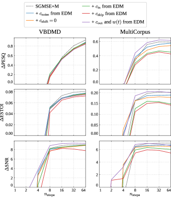
Figure 3: Speech enhancement performance as a function of the number of sampling steps ${n_{\mathrm{steps}}}$ for different preconditionings. The preconditioning parameters are incrementally set from the values in Eq. (41) used in [20, 21] to the values in Eq. (27) suggested in EDM [42].

Figure 3 shows the results of the preconditioning experiment. The speech enhancement performance is reported in terms of ${\Delta\text{\lx@glossaries@gls@link{acronym}{pesq}{\leavevmode PESQ} }}$, ${\Delta\text{\lx@glossaries@gls@link{acronym}{estoi}{\leavevmode ESTOI} }}$ and ${\Delta\text{\lx@glossaries@gls@link{acronym}{snr}{\leavevmode SNR} }}$ as a function of the number of sampling steps ${n_{\mathrm{steps}}}$. The dashed line corresponds to the SGMSE+M baseline from [43] and uses the preconditioning shown in Eq. (41). It can be seen that setting the ${c_{\mathrm{noise}}}$ parameter from ${\log t}$ to ${\frac{1}{4}\log\bar{\sigma}(t)}$ as suggested in EDM has a slight detrimental effect on performance, except on the MultiCorpus dataset for ${n_{\mathrm{steps}}\!\leq\!8}$ where the performance is higher. Similarly, setting ${c_{\mathrm{shift}}}$ to zero has a slight detrimental effect on performance. Subsequently setting ${c_{\mathrm{in}}}$ and ${c_{\mathrm{skip}}}$ to the values suggested in EDM also reduces performance. However, once ${c_{\mathrm{out}}}$ and ${w(t)}$ are set to the values suggested in EDM such that the full EDM preconditioning is used, the performance is recovered and is superior to the baseline for all metrics on the MultiCorpus dataset, except in terms of ${\Delta\text{\lx@glossaries@gls@link{acronym}{snr}{\leavevmode SNR} }}$ at ${n_{\mathrm{steps}}\!\geq\!32}$. For VBDMD, the performance is superior in terms of ${\Delta\text{\lx@glossaries@gls@link{acronym}{snr}{\leavevmode SNR} }}$ for all ${n_{\mathrm{steps}}}$ values, but remains inferior to the baseline in terms of ${\Delta\text{\lx@glossaries@gls@link{acronym}{pesq}{\leavevmode PESQ} }}$ and ${\Delta\text{\lx@glossaries@gls@link{acronym}{estoi}{\leavevmode ESTOI} }}$. Setting ${c_{\mathrm{out}}}$ to the value suggested in EDM without ${w(t)}$ led to training instabilities during our experiments, which is why results are not reported for this configuration.

V-B SDE

Figure 4: Speech enhancement performance as a function of the number of sampling steps ${n_{\mathrm{steps}}}$ for different SDEs .

(a) PC sampler

(b) EDM sampler

Figure 5: Speech enhancement performance as a function of the amount of stochasticity injected in the reverse process for different numbers of sampling steps ${n_{\mathrm{steps}}}$. For the PC sampler (a), the stochasticity is controlled by the step size of the annealed Langevin dynamics correction ${r}$. For the EDM sampler (b), this is controlled by the parameter ${S_{\mathrm{churn}}}$.

Figure 4 shows the results of the SDE experiment. The results show more variation compared to the preconditioning experiment, which suggests the noise schedule has a larger influence on performance compared to the preconditioning. It can be seen that the OUVE and OUVE₂ SDEs show very similar performance. This means that while we argue the OUVE₂ formulation is more practical, it does not lead to a performance improvement. More interestingly, the VE SDE shows similar performance to OUVE and OUVE₂, except in terms of ${\Delta\text{\lx@glossaries@gls@link{acronym}{snr}{\leavevmode SNR} }}$ for ${n_{\mathrm{steps}}\!\leq\!8}$. Since the VE SDE presents no drift of the diffusion process from the clean speech towards the noisy speech, this result suggests that the performance of diffusion-based speech enhancement cannot be attributed to such a drift as suggested in [20, 21]. Moreover, since the VE SDE imposes a substantially larger prior mismatch compared to OUVE and OUVE₂, this result also suggests that a prior mismatch is not necessarily responsible for a performance drop as suggested in [44]. Similar conclusions can be drawn when comparing the VP and OUVP SDEs . Indeed, they show similar performance at large ${n_{\mathrm{steps}}}$, and the VP SDE shows substantially higher performance at small ${n_{\mathrm{steps}}}$. This means that in this particular example, the drift of the diffusion process from the clean speech towards the noisy speech actually has a detrimental effect on performance, despite the reduced prior mismatch. The BBED SDE shows similar performance to the OUVE SDE on VBDMD and slightly lower performance on the MultiCorpus dataset. This is in opposition to [44], where the BBED SDE showed superior performance compared to the OUVE SDE on VBDMD, allegedly due to the reduced prior mismatch. We were unable to reproduce this result when using the EDM preconditioning and our training procedure. Finally, the cosine SDE shows significantly higher ${\Delta\text{\lx@glossaries@gls@link{acronym}{pesq}{\leavevmode PESQ} }}$ scores on VBDMD for ${n_{\mathrm{steps}}\!\geq\!8}$, but shows the lowest ${\Delta\text{\lx@glossaries@gls@link{acronym}{estoi}{\leavevmode ESTOI} }}$ and ${\Delta\text{\lx@glossaries@gls@link{acronym}{snr}{\leavevmode SNR} }}$ scores on the MultiCorpus dataset for ${n_{\mathrm{steps}}\!\geq\!8}$.

V-C Stochasticity injected in reverse process

Figure 5 shows the results of the stochasticity experiment. Figure 5a shows the results for the PC sampler as a function of the step size of the annealed Langevin dynamics correction ${r}$, while Fig. 5b shows the results for the EDM sampler as a function of the parameter ${S_{\mathrm{churn}}}$. The experiment is repeated for different numbers of sampling steps ${n_{\mathrm{steps}}}$. It can be seen that for the PC sampler, the step size ${r}$ has a large influence on performance. When using a small ${n_{\mathrm{steps}}}$, a sufficient and precise amount of stochasticity is required, as the curves present sharp maxima across all metrics. However, when increasing the number of sampling steps, the need for stochasticity is reduced, as the curves become flatter at low ${r}$ values. Large ${r}$ values have a detrimental effect on performance in both cases. For the EDM sampler, the parameter ${S_{\mathrm{churn}}}$ has a very small influence on performance, except for ${n_{\mathrm{steps}}\!=\!4}$. Nonetheless, a slight rising trend can be observed, which suggests that injecting as much stochasticity as possible in the reverse process is beneficial for the EDM sampler. However, as explained in Sect. IV-G3, the EDM sampler algorithm clamps the amount of noise injected in the reverse process, and we did not try removing this clamping. In [42], it was suggested that while the need for stochasticity reduces as the model improves, models trained with diverse datasets continue to benefit from stochasticity. Therefore, assuming these observations are valid for speech enhancement, our results suggest that the model can be further improved, or that the datasets are diverse enough.

V-D Comparison with baselines

Figure 6: Speech enhancement performance as a function of ${n_{\mathrm{steps}}}$ for two different sampler configurations and the baselines.

We set the preconditioning and the SDE as in the previous experiment. We chose between the PC sampler with ${r\!=\!0.5}$ as suggested in [21] and the EDM sampler with ${S_{\mathrm{churn}}\!=\!\infty}$. Figure 6 shows the performance of the two resulting systems and SGMSE+M as a function of the number of sampling steps ${n_{\mathrm{steps}}}$. We also plot the performance of the discriminative baselines as horizontal lines. When comparing our systems using both samplers, it can be seen that the EDM sampler shows superior performance compared to the PC sampler. This difference is the greatest when using few sampling steps. More specifically, the EDM sampler shows good performance on both datasets with only 4 sampling steps, while the PC sampler requires at least 16 sampling steps to achieve similar performance. This means the EDM sampler allows to reduce the computational cost by a factor of four without sacrificing performance. When comparing with SGMSE+M, it can be seen that our system using the EDM sampler outperforms the baseline in terms of ${\Delta\text{\lx@glossaries@gls@link{acronym}{pesq}{\leavevmode PESQ} }}$ and ${\Delta\text{\lx@glossaries@gls@link{acronym}{estoi}{\leavevmode ESTOI} }}$ for both datasets and all ${n_{\mathrm{steps}}}$ values, while SGMSE+M shows superior performance in terms of ${\Delta\text{\lx@glossaries@gls@link{acronym}{snr}{\leavevmode SNR} }}$ on VBDMD for ${n_{\mathrm{steps}}\!\geq\!16}$. We are thus able to outperform a previous diffusion-based system in terms of perceptual metrics at a substantially lower computational cost. Finally, while the discriminative baselines are competitive in terms of ${\Delta\text{\lx@glossaries@gls@link{acronym}{snr}{\leavevmode SNR} }}$ on both datasets, the three diffusion-based systems outperform them in terms of ${\Delta\text{\lx@glossaries@gls@link{acronym}{pesq}{\leavevmode PESQ} }}$ and ${\Delta\text{\lx@glossaries@gls@link{acronym}{estoi}{\leavevmode ESTOI} }}$ when using a large ${n_{\mathrm{steps}}}$.

VI Conclusion

In the present work, we extended the EDM framework proposed in [42] to include a recent diffusion-based speech enhancement model [20, 21]. Specifically, we considered a more general SDE with a non-zero long-term mean, we added a new parameter ${c_{\mathrm{shift}}}$ to the neural network preconditioning, and we showed that the score function can be evaluated on the unshifted and unscaled process instead of the unscaled process. This allowed to shed light on the different design aspects of diffusion models in the case of speech enhancement, and to apply recent developments from image generation literature that were not investigated for speech enhancement before.

By experimenting with SDEs that were not used for speech enhancement before, we were able to show that similar performance can be obtained with SDEs that present a drift from the clean speech towards the noisy speech compared to SDEs that do not present such a drift. This suggests that the model does not require such a drift to be able to perform the speech reconstruction task with environmental noises that differ from the stationary Gaussian noise of the diffusion process, contrary to previous beliefs [21]. This similar performance was observed despite the increased mismatch between the final distribution of the forward diffusion process and the prior distribution used to initialize the reverse process, even though this was argued to be responsible for a drop in performance [44]. Omitting the drift term makes the speech enhancement task fully generative, since this models a progressive transformation from Gaussian noise to clean speech, rather than from noisy speech to clean speech. Moreover, we hypothesize that this improves training efficiency, since the network does not need to learn to undo the scaling ${s(t)}$ before denoising.

The neural network preconditioning and the SDE had a smaller effect on performance compared to the sampler used to integrate the reverse process. In line with our previous work [45], the EDM sampler showed similar performance compared to the PC sampler while requiring fewer sampling steps. More specifically, it allowed for a fourfold decrease in computational cost, as it required as few as 4 sampling steps to perform similarly to the PC sampler with 16 sampling steps.

Despite the encouraging results, diffusion-based speech enhancement is still computationally more costly compared to state-of-the-art discriminative systems due to the multiple neural network evaluations in the reverse process. This raises the question of whether diffusion-based speech enhancement is worth the additional computational cost. While further reducing the computational cost is an obvious direction for future work, other options include systematically investigating the performance in mismatched conditions, or exploring the benefit of an unsupervised training procedure for speech enhancement. Indeed, the present work only investigated the performance in matched conditions, and while our previous study [45] reported results in mismatched conditions using multiple speech, noise and BRIR databases, this was not done in conjunction with the different design aspects of the diffusion model. It is thus unclear if some specific SDEs or the stochasticity in the reverse process are beneficial to generalizing to unseen acoustic conditions. Moreover, while the proposed diffusion-based approach is generative in that it learns a conditional probability distribution over clean speech, the models were trained in a supervised setting using pairs of clean and noisy speech signals. It would be interesting to investigate if an unsupervised training procedure improves the robustness to arbitrary additive and convolutional distortions.

Appendix A Cosine schedule parameters

Under the VP assumption, we have ${s^{2}\mskip-0.75mu(t)\!+\!\sigma^{2}\mskip-0.75mu(t)\!=\!1}$. Therefore, using Eqs. (9) and (16),

$$\textstyle s^{2}\mskip-0.75mu(t)+e^{-\lambda(t)}s^{2}\mskip-0.75mu(t)=1$$ (50)

$$\textstyle\implies \textstyle s^{2}\mskip-0.75mu(t)=\frac{1}{1+e^{-\lambda(t)}}=\frac{1}{1+e^{-2\nu}\tan^{2}\mskip-4.5mu\frac{\pi t}{2}}.$$ (51)

For ${\sigma(t)}$, we can reuse ${s^{2}\mskip-0.75mu(t)\!+\!\sigma^{2}\mskip-0.75mu(t)\!=\!1}$ such that

$$\textstyle\sigma^{2}\mskip-0.75mu(t) \textstyle=1-s^{2}\mskip-0.75mu(t)=1-\frac{1}{1+e^{-2\nu}\tan^{2}\mskip-4.5mu\frac{\pi t}{2}}$$ (52)

$$\textstyle=\frac{e^{-2\nu}\tan^{2}\mskip-4.5mu\frac{\pi t}{2}}{1+e^{-2\nu}\tan^{2}\mskip-4.5mu\frac{\pi t}{2}}=\frac{1}{1+e^{2\nu}\cos^{2}\mskip-4.5mu\frac{\pi t}{2}}.$$ (53)

The drift and diffusion coefficients ${f(t)}$ and ${g(t)}$ can be derived using Eqs. (8), (51) and (53). Specifically for ${f(t)}$,

$$\textstyle f(t) \textstyle=\frac{\mathop{}\!\mathrm{d}}{\mathop{}\!\mathrm{d}t}\big{[}\log s(t)\big{]}=\frac{\mathop{}\!\mathrm{d}}{\mathop{}\!\mathrm{d}t}\left[\log\sqrt{\frac{1}{1+e^{-2\nu}\tan^{2}\mskip-4.5mu\frac{\pi t}{2}}}\right]$$ (54)

$$\textstyle=-\frac{1}{2}\cdot\frac{\mathop{}\!\mathrm{d}}{\mathop{}\!\mathrm{d}t}\left[\log\left(1+e^{-2\nu}\tan^{2}\mskip-4.5mu\frac{\pi t}{2}\right)\right]$$ (55)

$$\textstyle=-\frac{1}{2}\cdot\frac{e^{-2\nu}}{1+e^{-2\nu}\tan^{2}\mskip-4.5mu\frac{\pi t}{2}}\cdot\frac{\mathop{}\!\mathrm{d}}{\mathop{}\!\mathrm{d}t}\left[\tan^{2}\mskip-4.5mu\frac{\pi t}{2}\right]$$ (56)

$$\textstyle=-\frac{1}{2}\cdot\frac{e^{-2\nu}}{1+e^{-2\nu}\tan^{2}\mskip-4.5mu\frac{\pi t}{2}}\cdot\frac{\pi\tan\!\frac{\pi t}{2}}{\cos^{2}\mskip-4.5mu\frac{\pi t}{2}}$$ (57)

$$\textstyle=-\frac{1}{2}\cdot\frac{e^{-2\nu}\tan^{2}\mskip-4.5mu\frac{\pi t}{2}}{1+e^{-2\nu}\tan^{2}\mskip-4.5mu\frac{\pi t}{2}}\cdot\frac{\pi}{\cos\!\frac{\pi t}{2}\sin\!\frac{\pi t}{2}}$$ (58)

$$\textstyle=-\frac{1}{1+e^{2\nu}\cos^{2}\mskip-4.5mu\frac{\pi t}{2}}\cdot\frac{\pi}{\sin(\pi t)}=-\frac{\pi\csc(\pi t)}{1+e^{2\nu}\cos^{2}\mskip-4.5mu\frac{\pi t}{2}}.$$ (59)

For ${g(t)}$, we can use the fact that under the VP assumption, we have ${g^{2}\mskip-0.75mu(t)\!=\!-2f(t)}$ from Eq. (13). Therefore,

$$\textstyle g(t)=\sqrt{\frac{2\pi\csc(\pi t)}{1+e^{2\nu}\cos^{2}\mskip-4.5mu\frac{\pi t}{2}}}.$$ (60)

Appendix B Proof of Eqs. (40) and (41)

We denote the unscaled noise as ${\bar{\boldsymbol{n}}_{t}\!=\!\bar{\sigma}(t)\boldsymbol{z}}$ and the scaled noise as ${\boldsymbol{n}_{t}\!=\!\sigma(t)\boldsymbol{z}\!=\!s(t)\bar{\sigma}(t)\boldsymbol{z}\!=\!s(t)\bar{\boldsymbol{n}}_{t}}$ where ${\boldsymbol{z}\!\sim\!\mathcal{N}_{\mathbb{C}}(0,\mskip-1.5mu\mathbf{I})}$. Similarly to [42], we start from the term inside the expectation operator in Eq. (33) and use the expression of the score model as a function of the raw neural network layers in Eq. (34),

(61)

$$\!=\scalebox{1.0}{$\left\|-\frac{\sigma(t)}{t}\boldsymbol{F}_{\boldsymbol{\theta}}\big{(}s(t)(\boldsymbol{x}_{0}-\boldsymbol{y})+\boldsymbol{y}+\boldsymbol{n}_{t},\boldsymbol{y},\log t\big{)}+\boldsymbol{z}\right\|_{2}^{2}$}\!\!\!\!\!\!\!$$ (62)

$$\!=\scalebox{1.0}{$\left\|-\frac{\sigma(t)}{t}\boldsymbol{F}_{\boldsymbol{\theta}}\big{(}s(t)\tilde{\boldsymbol{x}}_{0}+\boldsymbol{y}+s(t)\bar{\boldsymbol{n}}_{t},\boldsymbol{y},\log t\big{)}+\boldsymbol{z}\right\|_{2}^{2}$}\!\!\!\!\!\!\!$$ (63)

$$\!=\scalebox{0.96}{$\frac{1}{\bar{\sigma}^{2}\mskip-0.75mu(t)}\!\left\|-\frac{s(t)\bar{\sigma}^{2}\mskip-0.75mu(t)}{t}\boldsymbol{F}_{\boldsymbol{\theta}}\big{(}s(t)(\tilde{\boldsymbol{x}}_{0}\!+\!\bar{\boldsymbol{n}}_{t})\!+\!\boldsymbol{y},\boldsymbol{y},\log t\big{)}+\bar{\boldsymbol{n}}_{t}\right\|_{2}^{2}$}\!\!\!\!\!\!\!$$ (64)

$$\!=\scalebox{0.8}{$\frac{1}{\bar{\sigma}^{2}\mskip-0.75mu(t)}\!\left\|-\frac{s(t)\bar{\sigma}^{2}\mskip-0.75mu(t)}{t}\boldsymbol{F}_{\boldsymbol{\theta}}\big{(}s(t)(\tilde{\boldsymbol{x}}_{0}\!+\!\bar{\boldsymbol{n}}_{t})\!+\!\boldsymbol{y},\boldsymbol{y},\log t\big{)}\!+\!(\tilde{\boldsymbol{x}}_{0}\!+\!\bar{\boldsymbol{n}}_{t})\!-\!\tilde{\boldsymbol{x}}_{0}\right\|_{2}^{2}$}\!\!\!\!\!\!\!$$ (65)

$$\!=\scalebox{1.0}{$\mathop{\vtop{\halign{#\cr$\hfil\displaystyle{\textstyle\frac{1}{\bar{\sigma}^{2}\mskip-0.75mu(t)}}\hfil$\crcr\kern 3.0pt\nointerlineskip\cr\tiny\upbracefill\crcr\kern 1.0pt\cr}}}\limits_{w(t)}\left\|\boldsymbol{D}_{\boldsymbol{\theta}}(\tilde{\boldsymbol{x}}_{0}+\bar{\boldsymbol{n}}_{t},\boldsymbol{y},t)-\tilde{\boldsymbol{x}}_{0}\right\|_{2}^{2},$}\!\!\!\!\!\!\!$$ (68)

where ${w(t)}$ and the preconditioning become apparent,

Appendix C Proof of Eq. (42)

Starting from the definition of the marginal distribution and following similar steps as in Eqs. (15-19) in [42],

$$p_{t}(\boldsymbol{x}_{t}|\boldsymbol{y})=\int_{\mathbb{R}^{d}}p_{0t}(\boldsymbol{x}_{t}|\boldsymbol{x}_{0},\boldsymbol{y})p_{\mathrm{data}}(\boldsymbol{x}_{0})\mathop{}\!\mathrm{d}\boldsymbol{x}_{0}$$ (70)

$$\!\!=\int_{\mathbb{R}^{d}}\mathcal{N}\big{(}\boldsymbol{x}_{t};s(t)(\boldsymbol{x}_{0}-\boldsymbol{y})+\boldsymbol{y},\sigma^{2}\mskip-0.75mu(t)\mathbf{I}\big{)}p_{\mathrm{data}}(\boldsymbol{x}_{0})\mathop{}\!\mathrm{d}\boldsymbol{x}_{0}$$ (71)

$$\!\!=\int_{\mathbb{R}^{d}}\mathcal{N}\big{(}\boldsymbol{x}_{t}-\boldsymbol{y};s(t)(\boldsymbol{x}_{0}-\boldsymbol{y}),\sigma^{2}\mskip-0.75mu(t)\mathbf{I}\big{)}p_{\mathrm{data}}(\boldsymbol{x}_{0})\mathop{}\!\mathrm{d}\boldsymbol{x}_{0}$$ (72)

$$\!\!=\int_{\mathbb{R}^{d}}\mathcal{N}\big{(}\tilde{\boldsymbol{x}}_{t};s(t)\tilde{\boldsymbol{x}}_{0},\sigma^{2}\mskip-0.75mu(t)\mathbf{I}\big{)}p_{\mathrm{data}}(\tilde{\boldsymbol{x}}_{0}+y)\mathop{}\!\mathrm{d}\tilde{\boldsymbol{x}}_{0}$$ (73)

$$\!\!=s(t)^{-d}\int_{\mathbb{R}^{d}}\mathcal{N}\left(\frac{\tilde{\boldsymbol{x}}_{t}}{s(t)};\tilde{\boldsymbol{x}}_{0},\bar{\sigma}^{2}\mskip-0.75mu(t)\mathbf{I}\right)p_{\mathrm{data}}(\tilde{\boldsymbol{x}}_{0}+y)\mathop{}\!\mathrm{d}\tilde{\boldsymbol{x}}_{0}$$ (74)

$$\!\!=s(t)^{-d}\Big{[}\tilde{p}_{\mathrm{data},\boldsymbol{y}}\ast\mathcal{N}\big{(}\mathbf{0},\bar{\sigma}^{2}\mskip-0.75mu(t)\mathbf{I}\big{)}\Big{]}\left(\frac{\tilde{\boldsymbol{x}}_{t}}{s(t)}\right),$$ (75)

where ${\tilde{p}_{\mathrm{data},\boldsymbol{y}}:\boldsymbol{x}\mapsto p_{\mathrm{data}}(\boldsymbol{x}\!+\!\boldsymbol{y})}$ is a shifted version of ${p_{\mathrm{data}}}$ and ${\ast}$ is the convolution operator between PDFs .

References

- [1] A. K. Nabelek et al., “Monaural and binaural speech perception through hearing aids under noise and reverberation with normal and hearing-impaired listeners,” J. Speech Hear. Res., 1974.
- [2] ——, “Effect of noise and reverberation on binaural and monaural word identification by subjects with various audiograms,” J. Speech Lang. Hear. Res., 1981.
- [3] K. J. Palomäki et al., “A binaural processor for missing data speech recognition in the presence of noise and small-room reverberation,” Speech Commun., 2004.
- [4] T. May et al., “A binaural scene analyzer for joint localization and recognition of speakers in the presence of interfering noise sources and reverberation,” IEEE Audio, Speech, Lang. Process., 2012.
- [5] Y. Xu et al., “A regression approach to speech enhancement based on deep neural networks,” IEEE/ACM Trans. Audio, Speech, Lang. Process., 2015.
- [6] D. Wang et al., “Supervised speech separation based on deep learning: An overview,” IEEE/ACM Trans. Audio, Speech, Lang. Process., 2018.
- [7] T. Bentsen et al., “The benefit of combining a deep neural network architecture with ideal ratio mask estimation in computational speech segregation to improve speech intelligibility,” PLoS One, 2018.
- [8] P. Wang et al., “Bridging the gap between monaural speech enhancement and recognition with distortion-independent acoustic modeling,” IEEE/ACM Trans. Audio, Speech, Lang. Process., 2019.
- [9] I. Goodfellow et al., “Generative adversarial nets,” in Proc. NeurIPS, 2014.
- [10] D. P. Kingma et al., “Auto-encoding variational bayes,” in Proc. ICLR, 2014.
- [11] D. J. Rezende et al., “Variational inference with normalizing flows,” in Proc. ICML, 2015.
- [12] D. Michelsanti et al., “Conditional generative adversarial networks for speech enhancement and noise-robust speaker verification,” in Proc. INTERSPEECH, 2017.
- [13] Y. Bando et al., “Statistical speech enhancement based on probabilistic integration of variational autoencoder and non-negative matrix factorization,” in Proc. ICASSP, 2018.
- [14] A. A. Nugraha et al., “A flow-based deep latent variable model for speech spectrogram modeling and enhancement,” IEEE/ACM Trans. Audio, Speech, Lang. Process., 2020.
- [15] J. Sohl-Dickstein et al., “Deep unsupervised learning using nonequilibrium thermodynamics,” in Proc. ICML, 2015.
- [16] Y. Song et al., “Score-based generative modeling through stochastic differential equations,” in Proc. ICLR, 2021.
- [17] J. Ho et al., “Denoising diffusion probabilistic models,” in Proc. NeurIPS, 2020.
- [18] Y.-J. Lu et al., “A study on speech enhancement based on diffusion probabilistic model,” in Proc. APSIPA ASC, 2021.
- [19] ——, “Conditional diffusion probabilistic model for speech enhancement,” in Proc. ICASSP, 2022.
- [20] S. Welker et al., “Speech enhancement with score-based generative models in the complex STFT domain,” in Proc. INTERSPEECH, 2022.
- [21] J. Richter et al., “Speech enhancement and dereverberation with diffusion-based generative models,” IEEE/ACM Trans. Audio, Speech, Lang. Process., 2023.
- [22] H. Yen et al., “Cold diffusion for speech enhancement,” in Proc. ICASSP, 2023.
- [23] C. Chen et al., “Metric-oriented speech enhancement using diffusion probabilistic model,” in Proc. ICASSP, 2023.
- [24] H. Wang et al., “Cross-domain diffusion based speech enhancement for very noisy speech,” in Proc. ICASSP, 2023.
- [25] R. Sawata et al., “Diffiner: A versatile diffusion-based generative refiner for speech enhancement,” in Proc. INTERSPEECH, 2023.
- [26] P. Dhariwal et al., “Diffusion models beat GANs on image synthesis,” in Proc. NeurIPS, 2021.
- [27] R. Rombach et al., “High-resolution image synthesis with latent diffusion models,” in Proc. CVPR, 2022.
- [28] Z. Kong et al., “DiffWave: A versatile diffusion model for audio synthesis,” in Proc. ICLR, 2021.
- [29] V. Popov et al., “Grad-TTS: A diffusion probabilistic model for text-to-speech,” in Proc. ICML, 2021.
- [30] H. Liu et al., “AudioLDM: Text-to-audio generation with latent diffusion models,” in Proc. ICML, 2023.
- [31] J. Ho et al., “Video diffusion models,” in Proc. NeurIPS, 2022.
- [32] ——, “Imagen Video: High definition video generation with diffusion models,” arXiv preprint arXiv:2210.02303, 2022.
- [33] J.-M. Lemercier et al., “StoRM: A diffusion-based stochastic regeneration model for speech enhancement and dereverberation,” IEEE/ACM Trans. Audio, Speech, Lang. Process., 2023.
- [34] Z. Qiu et al., “SRTNET: Time domain speech enhancement via stochastic refinement,” in Proc. ICASSP, 2023.
- [35] B. Kawar et al., “Denoising diffusion restoration models,” in Proc. NeurIPS, 2022.
- [36] J. Whang et al., “Deblurring via stochastic refinement,” in Proc. CVPR, 2022.
- [37] H. Chung et al., “Improving diffusion models for inverse problems using manifold constraints,” in Proc. NeurIPS, 2022.
- [38] ——, “Diffusion posterior sampling for general noisy inverse problems,” in Proc. ICLR, 2023.
- [39] E. Moliner et al., “Solving audio inverse problems with a diffusion model,” in Proc. ICASSP, 2023.
- [40] J.-M. Lemercier et al., “Diffusion posterior sampling for informed single-channel dereverberation,” in Proc. WASPAA, 2023.
- [41] A. Iashchenko et al., “UnDiff: Unsupervised voice restoration with unconditional diffusion model,” in Proc. INTERSPEECH, 2023.
- [42] T. Karras et al., “Elucidating the design space of diffusion-based generative models,” in Proc. NeurIPS, 2022.
- [43] J.-M. Lemercier et al., “Analysing diffusion-based generative approaches versus discriminative approaches for speech restoration,” in Proc. ICASSP, 2023.
- [44] B. Lay et al., “Reducing the prior mismatch of stochastic differential equations for diffusion-based speech enhancement,” in Proc. INTERSPEECH, 2023.
- [45] P. Gonzalez et al., “Diffusion-based speech enhancement in matched and mismatched conditions using a heun-based sampler,” arXiv preprint arXiv:2312.02683, 2023.
- [46] B. D. Anderson, “Reverse-time diffusion equation models,” Stochastic Processes and their Applications, 1982.
- [47] A. Hyvärinen, “Estimation of non-normalized statistical models by score matching,” J. Mach. Learn. Res., 2005.
- [48] P. Vincent, “A connection between score matching and denoising autoencoders,” Neural Comput., 2011.
- [49] Y. Song et al., “Sliced score matching: A scalable approach to density and score estimation,” in Proc. UAI, 2020.
- [50] S. Särkkä et al., Applied stochastic differential equations. Cambridge University Press, 2019, vol. 10.
- [51] D. P. Kingma et al., “Variational diffusion models,” in Proc. NeurIPS, 2021.
- [52] T. Salimans et al., “Progressive distillation for fast sampling of diffusion models,” in Proc. ICLR, 2022.
- [53] E. Hoogeboom et al., “simple diffusion: End-to-end diffusion for high resolution images,” in Proc. ICML, 2023.
- [54] D. P. Kingma et al., “Understanding diffusion objectives as the ELBO with simple data augmentation,” in Proc. NeurIPS, 2023.
- [55] A. Nichol et al., “Improved denoising diffusion probabilistic models,” in Proc. ICML, 2021.
- [56] G. E. Uhlenbeck et al., “On the theory of the brownian motion,” Physical review, 1930.
- [57] Z. Guo et al., “Variance-preserving-based interpolation diffusion models for speech enhancement,” in Proc. INTERSPEECH, 2023.
- [58] C. Valentini-Botinhao et al., “Speech enhancement for a noise-robust text-to-speech synthesis system using deep recurrent neural networks,” in Proc. INTERSPEECH, 2016.
- [59] C. Veaux et al., “The Voice Bank corpus: Design, collection and data analysis of a large regional accent speech database,” in Proc. O-COCOSDA/CASLRE, 2013.
- [60] J. Thiemann et al., “The diverse environments multi-channel acoustic noise database (DEMAND): A database of multichannel environmental noise recordings,” in Proc. Mtgs. Acoust., 2013.
- [61] P. Gonzalez et al., “Assessing the generalization gap of learning-based speech enhancement systems in noisy and reverberant environments,” IEEE/ACM Trans. Audio, Speech, Lang. Process., 2023.
- [62] J. S. Garofolo et al., “DARPA TIMIT acoustic-phonetic continuous speech corpus CD-ROM, NIST speech disc 1-1.1,” National Institute of Standards and Technology, Gaithersburg, MD, 1993.
- [63] V. Panayotov et al., “LibriSpeech: An ASR corpus based on public domain audio books,” in Proc. ICASSP, 2015.
- [64] D. B. Paul et al., “The design for the Wall Street Journal-based CSR corpus,” in Proc. Workshop Speech Natural Lang., 1992.
- [65] S. Graetzer et al., “Dataset of British English speech recordings for psychoacoustics and speech processing research: The Clarity speech corpus,” Data in Brief, 2022.
- [66] T. Heittola et al., “TAU urban acoustic scenes 2019, development dataset,” 2019. https://doi.org/10.5281/zenodo.2589280
- [67] A. Varga et al., “Assessment for automatic speech recognition: II. NOISEX-92: A database and an experiment to study the effect of additive noise on speech recognition systems,” Speech Commun., 1993.
- [68] W. A. Dreschler et al., “ICRA noises: Artificial noise signals with speech-like spectral and temporal properties for hearing instrument assessment,” Audiology, 2001.
- [69] A. Weisser et al., “The ambisonic recordings of typical environments (ARTE) database,” Acta Acustica United With Acustica, 2019.
- [70] C. Hummersone et al., “Dynamic precedence effect modeling for source separation in reverberant environments,” IEEE Audio, Speech, Lang. Process., 2010.
- [71] S. Pearce, “Audio Spatialisation for Headphones - Impulse Response Dataset,” 2021. https://doi.org/10.5281/zenodo.4780815
- [72] F. Brinkmann et al., “A benchmark for room acoustical simulation. Concept and database,” Applied Acoustics, 2021.
- [73] “Simulated room impulse responses,” University of Surrey. http://iosr.surrey.ac.uk/software/index.php#CATT_RIRs
- [74] L. McCormack et al., “Higher-order spatial impulse response rendering: Investigating the perceived effects of spherical order, dedicated diffuse rendering, and frequency resolution,” J. Audio Eng. Soc., 2020.
- [75] N. Roman et al., “Speech intelligibility in reverberation with ideal binary masking: Effects of early reflections and signal-to-noise ratio threshold,” J. Acoust. Soc. Am., 2013.
- [76] P. Zahorik, “Direct-to-reverberant energy ratio sensitivity,” J. Acoust. Soc. Am., 2002.
- [77] O. Ronneberger et al., “U-Net: Convolutional networks for biomedical image segmentation,” in Proc. MICCAI, 2015.
- [78] D. P. Kingma et al., “Adam: A method for stochastic optimization,” in Proc. ICLR, 2015.
- [79] P. Gonzalez et al., “On batching variable size inputs for training end-to-end speech enhancement systems,” in Proc. ICASSP, 2023.
- [80] Y. Song et al., “Improved techniques for training score-based generative models,” in Proc. NeurIPS, 2020.
- [81] Y. Luo et al., “Conv-TasNet: Surpassing ideal time-frequency magnitude masking for speech separation,” IEEE/ACM Trans. Audio, Speech, Lang. Process., 2019.
- [82] Y. Hu et al., “DCCRN: Deep complex convolution recurrent network for phase-aware speech enhancement,” in Proc. INTERSPEECH, 2020.
- [83] H. J. Park et al., “MANNER: Multi-view attention network for noise erasure,” in Proc. ICASSP, 2022.
- [84] Y. Koyama et al., “Exploring the best loss function for DNN-based low-latency speech enhancement with temporal convolutional networks,” arXiv preprint arXiv:2005.11611, 2020.
- [85] K. Kinoshita et al., “Improving noise robust automatic speech recognition with single-channel time-domain enhancement network,” in Proc. ICASSP, 2020.
- [86] J. Le Roux et al., “SDR – half-baked or well done?” in Proc. ICASSP, 2019.
- [87] C. Trabelsi et al., “Deep complex networks,” in Proc. ICLR, 2018.
- [88] S. Hochreiter et al., “Long short-term memory,” Neural Comput., 1997.
- [89] S. Ioffe et al., “Batch normalization: Accelerating deep network training by reducing internal covariate shift,” in Proc. ICML, 2015.
- [90] H. Wu et al., “Rethinking complex-valued deep neural networks for monaural speech enhancement,” in Proc. INTERSPEECH, 2023.
- [91] S. Woo et al., “CBAM: Convolutional block attention module,” in Proc. ECCV, 2018.
- [92] Y. Luo et al., “Dual-path RNN: Efficient long sequence modeling for time-domain single-channel speech separation,” in Proc. ICASSP, 2020.
- [93] R. Yamamoto et al., “Parallel WaveGAN: A fast waveform generation model based on generative adversarial networks with multi-resolution spectrogram,” in Proc. ICASSP, 2020.
- [94] A. Défossez et al., “Real time speech enhancement in the waveform domain,” in Proc. INTERSPEECH, 2020.
- [95] L. N. Smith et al., “Super-convergence: Very fast training of neural networks using large learning rates,” in Artificial intelligence and machine learning for multi-domain operations applications, 2019.
- [96] Perceptual evaluation of speech quality (PESQ): An objective method for end-to-end speech quality assessment of narrow-band telephone networks and speech codecs, Rec. ITU-T P.862, International Telecommunication Union, 2001.
- [97] J. Jensen et al., “An algorithm for predicting the intelligibility of speech masked by modulated noise maskers,” IEEE/ACM Trans. Audio, Speech, Lang. Process., 2016.