The charge density and neutron skin thickness of Skyrmions

Abstract

Motivated by recent parity violating electron scattering experiments, we compute the Neutron Skin Thickness (NST) of nuclei modelled as (quantized) Skyrmions, the topological solitons of the Skyrme model. We show how in a certain approximation, the result for the NST is oblivious to the fine details of the (generally very complicated) quantum state of the soliton and only depends on the total baryon number and the isospin number. Moreover, in the leading order, the linear dependence on the asymmetry parameter is recovered, as expected both from experimental data and other models of nuclei such as the liquid drop model.

I Introduction

Some properties of nuclei, such as the energies of their quantum ground states and their charge radii, have long been experimentally measured with outstanding accuracy. In particular, electromagnetic Form Factors (FFs), which describe how the nucleon target reacts in an elastic scattering with an electrically charged (usually leptonic) probe and contain information about the internal distribution of charge and magnetization within nuclei, have been used to determine the nuclear structure for more than fifty years Hofstadter (1956). Electromagnetic FFs of nucleons and nuclei have been measured over the last decades in elastic electron scattering experiments with an increasing precision De Jager et al. (1974); Perdrisat et al. (2007), reaching an impressive level recently at JLab Punjabi et al. (2015); Camsonne et al. (2014); Arrington et al. (2023) even for large momentum transfer.

Since they were first proposed, it has been customary to interpret FFs as the Fourier transforms of local spatial distributions. However, relativistic wave functions are frame-dependent, and hence such an interpretation is often restricted to the Breit frame Sachs (1962). Recently, the generalization of this interpretation to an arbitrary, relativistic reference frame was proposed in Lorcé (2020) by introducing an appropriate kinematic factor in the Fourier integral (which also resolves the apparent contradiction between the same magnitude obtained in the Breit and infinite momentum frames Miller (2007)).

The issue of whether it makes sense to define a localized charge density for quantum objects such as nucleons has also been subject to some debate Jaffe (2021). This ambiguity was recently resolved in Epelbaum et al. (2022), where a redefinition of the charge density in terms of a new integral involving the electric form factor was shown to not depend on the particular wavefunction, as long as one can assume its spherical symmetry, i.e. in the rest frame of the system.

Therefore, an accurate description of the local charge densities of nucleons, and especially of the proton, has become one of the main goals of theoretical nuclear physics. The description is not only essential to the knowledge of strong forces in the non-perturbative regime but also to the understanding of other precision observables in quantum electrodynamics Gao and Vanderhaeghen (2022) and other fundamental interactions, including gravity Polyakov and Schweitzer (2018). However, compared to electromagnetic charge densities, other properties of nuclei, such as the neutron spatial distribution, are even less known experimentally. Indeed, while the proton distribution is explored through electromagnetic probes (charged leptons), whose interactions are well understood from the theory of quantum electrodynamics, the distribution of neutrons has been explored mainly through hadronic probes such as pions Krasznahorkay et al. (2004) or heavy ions Xu (2023); Li et al. (2020). These are described by quantum chromodynamics, which is subject to large uncertainties in the low energy regime due to its non-perturbative nature.

Both kinds of charge densities are a valuable source of information about the internal structure of nuclei and the strong force. The distribution of charges inside a nucleus can reveal information about the isospin-asymmetric nuclear forces Mondal et al. (2016). It turns out that these are crucial to the understanding of matter inside compact stars, and play a relevant role in the nuclear matter Equation of State Lattimer (2023).

A related observable is the neutron skin thickness (NST), defined as the difference between the mean square radius of neutrons and that of protons, i.e.

$$\Delta R_{np}(^{B}X)=R_{n}-R_{p},\qquad R_{n}=\sqrt{\frac{\int\rho_{n}r^{2}d^{3}x}{B-Z}},\quad R_{p}=\sqrt{\frac{\int\rho_{p}r^{2}d^{3}x}{Z}},$$ (1)

where $R_{n\,(p)}$ represents the root mean square (rms) radius of the point neutron (proton) distributions, $\rho_{n(p)}$. The NST has been discussed for a long time in the nuclear physics literature (for a recent review on the topic see eg. Sammarruca (2023)). Traditionally, theoretical discussions on the NST have not been enough to determine its structure in a model-independent fashion, and the difficulty of observing the neutron distribution experimentally translated into a poor understanding of the quantity.

However, there has recently been an increased interest in the NST since parity-violating electron scattering (PVES) experiments aiming to observe the neutron distribution of ${}^{208}\rm Pb$ Adhikari et al. (2021) and ${}^{48}\rm Ca$ Adhikari et al. (2022) have been successfully performed. In such experiments, an electron is scattered off a nucleus, and the tiny asymmetry between right and left-handed scattered leptons due to parity-non conservation of the weak force is measured. The measurement of the parity violating asymmetry in polarized scattering allows one to determine the nuclear weak charge form factor, interpreted as the Fourier transform of the weak charge density for a given momentum transfer, that is also strongly correlated with the neutron distribution (since the weak neutral coupling of protons is much smaller than that of neutrons at low momentum transfer, i.e $Q^{p}_{W}=1-4\sin^{2}\theta_{W}\approx 0.075\ll Q^{n}_{W}=-1$). Although such measurements avoid strong interaction uncertainties by using leptonic probes, they are technically very challenging as they are based on a very small effect, of order about a part per million Horowitz et al. (2001); Roca-Maza et al. (2011).

Additionally, other leptonic probes can be used to study the weak charge distribution on nuclei. In particular, experiments involving neutrinos, whose interaction with nuclear matter is purely mediated by neutral weak bosons, have been proposed in order to measure the neutron density distribution of nuclei via the so-called Coherent Elastic neutrino-Nucleus Scattering (CEvNS) Freedman (1974); Patton et al. (2012); Payne et al. (2019). As opposed to the PVES, in which the scattered electrons are measured, the outgoing neutrinos are impossible to detect. Instead, what is measured is the very low kinetic energy of the recoiling nucleus. Due to the difficulty of such measurement, its experimental realization had to wait four decades, until the COHERENT collaboration was able to observe CEvNS Akimov et al. (2017) (see also Akimov et al. (2021)).

Inspired by this recent experimental progress, we will use the Skyrme model to compute the neutron skin thickness of nuclei with arbitrary size and isospin, in the limit of small isospin asymmetry (i.e. small ratio of protons versus neutrons). In the Skyrme model approach, nuclei are semi-classical objects: one starts with a classical, localized topological soliton solution (called Skyrmions), and first quantizes its zero-modes to find the allowed quantum states representing physical nuclear states. This is the so-called rigid rotor quantization. Using this approximation, the calculation of the charge densities and radius for the lightest nuclei, such as the $B=2$ (deuteron) and $B=3$ (triton and helium-3) solutions was performed more than thirty years ago Braaten and Carson (1989); Carson (1991a). Although the Skyrme model provides a systematic way of obtaining quantum states and their corresponding charge densities for larger nuclei, in practice the computations become very involved for sufficiently large baryon number, hence there have been very little progress in the study of local charge densities for large nuclei from the Skyrme model approach. Some limited investigations have been performed involving magnitudes that do not require quantization, such as the charge densities of isospin-zero states Karliner et al. (2016) or gravitational form factors Garcia Martin-Caro et al. (2023). However, large, neutron-rich nuclei are precisely the most interesting to experimentally determine properties involving isospin asymmetric pat of nuclear interactions, such as the NST.

In this paper, we use the rigid rotor approximation and find an expression for the NST that only depends on simple properties of the classical solutions, (and not on the complicated details of the quantum states) which are easily computed numerically. This result can be derived directly without doing any intermediate steps involving the associated form factors, therefore avoiding the above-mentioned problems with their interpretation as Fourier transforms of real densities.

II The Skyrme model: Skyrmions as nuclei

The Skyrme model that we consider is given by the following Lagrangian density,

$$\mathcal{L}_{\rm SK}=-\frac{f_{\pi}^{2}}{16\hbar}\Tr\{L_{\mu}L^{\mu}\}+\frac{\hbar}{32e^{2}}\Tr\{[L_{\mu},L_{\nu}]^{2}\}+\frac{m_{\pi}^{2}f_{\pi}^{2}}{8\hbar^{3}}\Tr\{U-\bm{1}\},$$ (2)

where we use the metric convention $\eta^{\mu\nu}={\rm diag}(1,-1,-1,-1)$. $U\in SU(2)$ contains the fundamental mesonic degrees of freedom, parametrized as the coordinates of the $SU(2)$ group element

$$U=\sigma\bm{1}+i\pi_{a}\tau_{a}\equiv i\phi^{\alpha}\bar{\tau}_{\alpha},\quad\phi^{\alpha}=(\sigma,\bm{\pi}),\quad\bar{\tau}_{\alpha}=(-i\bm{1},\bm{\tau}),$$ (3)

with $\tau^{a}$ ($a=1,2,3$) being the Pauli matrices. The left-currents $L_{\mu}=U^{\dagger}\partial_{\mu}U$ are the components of the associated left-invariant Maurer-Cartan form, $\bm{1}$ is the $2\times 2$ identity matrix, and $B^{\mu}$ is the topological current,

$$B^{\mu}=\frac{\epsilon^{\mu\nu\rho\sigma}}{24\pi^{2}}\Tr\{L_{\nu}L_{\rho}L_{\sigma}\}.$$ (4)

The integral of the zeroth element of the current is equal to the topological charge of the skyrmion

$$B=\int B^{0}(x)\,d^{3}x=\int\frac{\epsilon^{ijk}}{24\pi^{2}}\Tr\{L_{i}L_{j}L_{k}\}\,d^{3}x\in\mathbb{Z}\,.$$ (5)

We will consider static solutions of the Skyrme field and for numerical purposes, we adopt the usual Skyrme units of energy and length,

$$E_{s}=\frac{f_{\pi}}{4e},\quad x_{s}=\frac{2\hbar}{f_{\pi}e},$$ (6)

and use the dimensionless pion mass

$$m=\frac{2m_{\pi}}{f_{\pi}e}\,.$$ (7)

The static energy functional in these units becomes

$$E[U]=\int d^{3}x\left[-\frac{1}{2}\Tr\left\{L_{i}L_{i}\right\}-\frac{1}{16}\Tr\left\{\left[L_{i},L_{j}\right]\left[L_{i},L_{j}\right]\right\}+m^{2}\Tr\{\bm{1}-U\}\right]\,.$$ (8)

II.1 Quantization

Nucleons and nuclei are described within the Skyrme model as classical solitonic configurations through the identification of the Skyrmion topological charge with the baryon number of nuclear states. However, other quantum numbers such as the spin and isospin of quantum nuclear states are not described at the classical level. Hence, a quantization of the Skyrmion field is needed to take into account the relevant quantum numbers. This is done in the semi-classical approach by promoting the zero modes of the soliton to dynamical degrees of freedom.

To do so, we introduce the rotational and iso-rotational degrees of freedom through a pair of time-dependent $SU(2)$ transformations of the classical (static) solitonic solution, representing the iso-rotation and the spatial rotation zero modes, respectively,

$$U(t,\bm{x})=A(t)U_{0}(R_{B}(t)(\bm{x}))A^{\dagger}(t)\,,$$ (9)

where $R^{ij}_{B}=\tfrac{1}{2}\Tr{\tau^{i}B\tau^{j}B^{\dagger}}\in SO(3)$ is the corresponding rotation matrix in space. $A(t),B(t)\in SU(2)$ form the collective coordinates of the soliton. We note that, for spherically symmetric solutions, rotation in coordinate space can be undone by that in isospin space, reducing the effective number of independent degrees of freedom Adkins et al. (1983). However, the present treatment is more general and can also be used for non-spherical solutions that we shall be mainly interested in. The semi-classical quantization of the Skyrmion then consists of substituting (9) into the Skyrme Lagrangian (2), which yields the Lagrangian of an effective dynamical system in terms of the collective coordinates $\{A(t),B(t)\}$, and quantizing such a system via standard canonical methods. Performing the substitution yields the following Lagrangian

$$L_{\rm col}=\int d^{3}x\mathcal{L}_{\rm SK}=-E[U_{0}]+\frac{1}{2}a_{i}U_{ij}a_{j}-a_{i}W_{ij}b_{j}+\frac{1}{2}b_{i}V_{ij}b_{j},$$ (10)

where

$$a_{j}=-i\operatorname{Tr}\tau_{j}A^{-1}\dot{A},\quad b_{j}=i\operatorname{Tr}\tau_{j}\dot{B}B^{-1}$$

are the angular velocities in isospace and physical space, respectively. We have also introduced the corresponding $3\times 3$ inertia tensors $U,W$ and $V$ defined by

$$\Lambda=\begin{pmatrix}U&W\\ W^{T}&V\end{pmatrix},\quad\Lambda_{ij}=-\int\frac{1}{2}\text{Tr}\left(G_{i}G_{j}\right)+\frac{1}{8}\text{Tr}\left([L_{k},G_{i}][L_{k},G_{j}]\right)d^{3}x\,,$$ (11)

where $G_{i}=iG_{ia}\tau_{a}$ is an $\mathfrak{su}(2)$ current equal to

$$G_{i}=\begin{cases}\tfrac{i}{2}U_{0}^{\dagger}[\tau_{i},U_{0}]\,,\quad&i=1,2,3\\ \epsilon_{ilm}x_{l}L_{m}\,,\quad&i=4,5,6\,,\,.\end{cases}$$ (12)

For notational simplicity, here and below we do not distinguish upper ($x^{i},\tau^{a}$) from lower ($x_{i},\tau_{a}$) indices for three-dimensional vectors and tensors when we deal with purely three-dimensional expressions.

The quantum operators of the angular velocities $a_{j}$ and $b_{j}$ correspond to the rotational and iso-rotational collective coordinates $A,B$ and their canonically conjugate momenta, the body-fixed isospin and spin angular momentum operators $K_{j}$ and $L_{j}$. These are obtained in terms of the angular velocities via the relations,

$$K_{i} =U_{ij}a_{j}-W_{ij}b_{j}$$ (13)

$$L_{i} =-W_{ji}a_{j}+V_{ij}b_{j}\,.$$

These operators are related to the usual space-fixed isospin and spin angular momentum operators $I_{j}$ and $J_{j}$ via

$$I_{i}=-R_{ij}(A)K_{j},\quad J_{i}=-R_{ij}\left(B\right)^{T}L_{j}$$ (14)

implying $\bm{I}^{2}=\mathbf{K}^{2}$ and $\bm{J}^{2}=\mathbf{L}^{2}$. The set of operators, $\bm{I},\bm{J},\bm{K}$ and $\bm{L},$ form an irreducible representation of the Lie algebra of $\mathcal{O}_{I,K}\otimes\mathcal{O}_{L_{n}J},$ the symmetry group of two rigid rotators, and obey the commutation relations

$${\left[I_{i},I_{j}\right]=i\epsilon_{ijk}I_{k},}\quad{\left[K_{i},K_{j}\right]=i\epsilon_{ijk}K_{k}},\quad{\left[J_{i},J_{j}\right]=i\epsilon_{ijk}J_{k1}},\quad{\left[L_{i},L_{j}\right]=i\epsilon_{i,jk}L_{k}}.$$ (15)

From these, we may produce a complete set of commuting observables to define an eigenstate basis of $\mathcal{H}_{G}$. We construct such a basis with states of the form

$$\ket{G}=\ket{i,i_{3},k_{3}}\otimes\ket{j,j_{3},l_{3}}\equiv\ket{i,i_{3},k_{3};j,j_{3},l_{3}}$$ (16)

where $j$ and $j_{3}$ correspond to the eigenvalues of the corresponding total angular momentum and the third component of angular momentum operators, where $-i\leq i_{3},k_{3}\leq i$ and $-j\leq j_{3},l_{3}\leq j.$ In particular, the subspace we will be mostly interested in is that of fixed $i,i_{3},j,j_{3}$, labeled by the states $\ket{k_{3},l_{3}},$ which is $(2i+1)(2j+1)-$dimensional.

III The electric charge density of Skyrmions

The Gell-Mann-Nishijima formula tells us how to obtain the charge density of a Skyrmion field configuration,

$$Z=\frac{1}{2}B+I_{3}\hskip 5.69054pt\longrightarrow\hskip 5.69054pt\rho=\frac{1}{2}B^{0}+\expectationvalue{I^{0}_{3}},$$ (17)

where $I^{0}_{3}$ is the time-like component of the third isospin Noether current, and the brackets represent the expectation value on the quantum state of the Skyrmion. An explicit expression for (the classical version of) this current can be obtained from Noether’s theorem, given that an infinitesimal isospin transformation

$$U\rightarrow U^{\prime}=U+\epsilon^{k}\delta U_{k},\qquad\delta U_{k}=\frac{i}{2}[\tau^{k},U],$$ (18)

generates the Noether current

$$I^{\mu}_{k}=-\frac{1}{24\pi^{2}}\big{[}\Tr{L^{\mu}G_{k}}+\Tr{\left[L_{\nu},L^{\mu}\right]\left[L^{\nu},G_{k}\right]}\big{]},$$ (19)

where $G_{k}$ is the $\mathfrak{su}(2)$ current defined in eq. 12 ($k=1,2,3$).

The quantum version of $I_{3}^{0}$ can be obtained in rigid-rotor quantization by substituting the dynamical ansatz (9) into (19). One then replaces the classical variable $a_{i}$ with the corresponding quantum operators and applies Weyl ordering to the products of two or more non-commuting operators Carson (1991a). In the case of the angular velocity, we will use the quantum (body-fixed) angular momentum operators i.e. we need to invert (13). This simplifies significantly if we assume that the moment of inertia tensors satisfy the following sphericity condition:

$$U_{ij}=u\delta_{ij},\quad V_{ij}=v\delta_{ij},\quad W_{ij}=w\delta_{ij}.$$ (20)

i.e, the tensors defined in eq. 11 are proportional to the identity. This is true for the $B=1,3$ skyrmions and can be a good approximation for large skyrmions. Indeed, eq. 20 deals with quantities defined on the internal isospin space, and can be a good approximation even for highly non-spherical solutions in real space, as we show in the next section.

The expectation value of $I_{3}^{0}$ in the isospin state $\ket{\psi}$ is then given by

$$\expectationvalue{I_{3}^{0}}= -\frac{1}{(uv-w^{2})}\bra{\psi}\quantity[R_{3a}u_{ab}(vK^{b}+wL^{b})-R_{3a}w_{ab}(wK^{b}+uL^{b})]_{\rm Weyl}\ket{\psi}=$$

$$= -\frac{1}{2}\bra{\psi}\quantity[\frac{(u-v)u_{ab}+(u-w)w_{ab}}{(uv-w^{2})}[R_{3a}K_{b}]_{+}+\frac{wu_{ab}+uw_{ab}}{(uv-w^{2})}[R_{3a},M_{b}]_{+}]\ket{\psi}$$ (21)

where we have used the relation between the body-fixed and space-fixed angular momenta (14), and defined the grand spin operator $M_{i}=K_{i}+L_{i}$. The non-trivial part of the calculation is to compute the matrix elements

$$\mathcal{M}_{ab}(\psi)=\frac{1}{2}\bra{\psi}[R_{3a},K_{b}]_{+}\ket{\psi},\qquad\tilde{\mathcal{M}}_{ab}(\psi)=\frac{1}{2}\bra{\psi}[R_{3a},M_{b}]_{+}\ket{\psi}\,.$$ (22)

If this can be done, one can obtain the charge density of the skyrmion in any given quantum state $\ket{\psi}$.

In the case of nucleons, spherical symmetry implies $u=v=w$, so eq. 21 is undefined. To get rid of the apparent divergence we can rewrite the denominator as

$$\lim\limits_{v,w\to u}uv-w^{2}=(u+u)(u-u)$$ (23)

and the term $(u-u)$ cancels with the same term in the denominator, once we take into account the fact that nucleons are grand spin singlets, i.e. satisfy $\vec{L}\ket{\psi}=-\vec{K}\ket{\psi}$. Therefore, for nucleon states $\ket{\psi}=\ket{\frac{1}{2},i_{3},j_{3}}$ Braaten et al. (1986), the expectation of $I^{0}_{3}$ is

$$\expectationvalue{I^{0}_{3}}{\psi}=-\frac{u_{ij}}{2u}\bra{\tfrac{1}{2},i_{3},j_{3}}[R_{3j}K_{i}]_{+}\ket{\tfrac{1}{2},i_{3},j_{3}}=-\frac{u_{ij}}{6u}\delta^{ij}\expectationvalue{\tau^{3}}{i_{3}}\innerproduct{j_{3}}{j_{3}}\,.$$ (24)

Thus the charge density of quantized $B=1$ Skyrmions in the ground state is given by

$$\rho(\vec{x};i_{3})=\frac{1}{2}B^{0}(r)-i_{3}\frac{\delta^{ij}u_{ij}(r)}{3u}$$ (25)

which preserves spherical symmetry.

In fig. 1 we plot the radial profile of the charge densities for protons and neutrons as predicted by the Skyrme model. The dotted line data is calculated from the nucleon form factors, using an improved definition of the charge density Epelbaum et al. (2022).

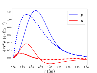
Figure 1: Radial profile of the electric charge density of nucleons

This method can be generalized to certain higher baryon charges. The $3-$skyrmion also obeys the sphericity condition (20). The ground state of its physical Hilbert space is the spin $\tfrac{1}{2}$, $(^{3}{\rm H},^{3}{\rm He})$ isospin doublet Manko et al. (2007); Carson (1991b),

$$\ket{\psi}\equiv\ket{{}^{3}{\rm H}/^{3}{\rm He},s}=\ket{\tfrac{1}{2},s,\tfrac{1}{2}}\ket{\tfrac{1}{2},\nicefrac{{+}}{{-}}\tfrac{1}{2},\tfrac{-1}{2}}-\ket{\tfrac{1}{2},s,\tfrac{-1}{2}}\ket{\tfrac{1}{2},\nicefrac{{+}}{{-}}\tfrac{1}{2},\tfrac{1}{2}}.$$ (26)

The states are grand spin singlet, so $\tilde{M}_{ij}$ will vanish, and we have

$$\bra{\psi}I_{3}^{0}(\vec{x})\ket{\psi} =-\mathcal{M}_{ab}(\psi)\frac{(v-w)u_{ab}(\vec{x})+(u-w)w_{ab}(\vec{x})}{(uv-w^{2})},$$ (27)

$$\rho(\vec{x},\psi)=\frac{1}{2}B_{0}(\vec{x})+\bra{\psi}I_{3}^{0}(\vec{x})\ket{\psi} =\frac{1}{2}B_{0}(\vec{x})-i_{3}\delta_{ab}\frac{(v-w)u_{ab}(\vec{x})+(u-w)w_{ab}(\vec{x})}{3(uv-w^{2})}.$$ (28)

The charge densities of ${}^{3}{\rm H}$ and ${}^{3}{\rm He}$ ground states in the Skyrme model are not spherically symmetric, but preserve the tetrahedral symmetry of the classical solution (as required by the FR constraints). We plot a two-dimensional projection of these densities in fig. 2.

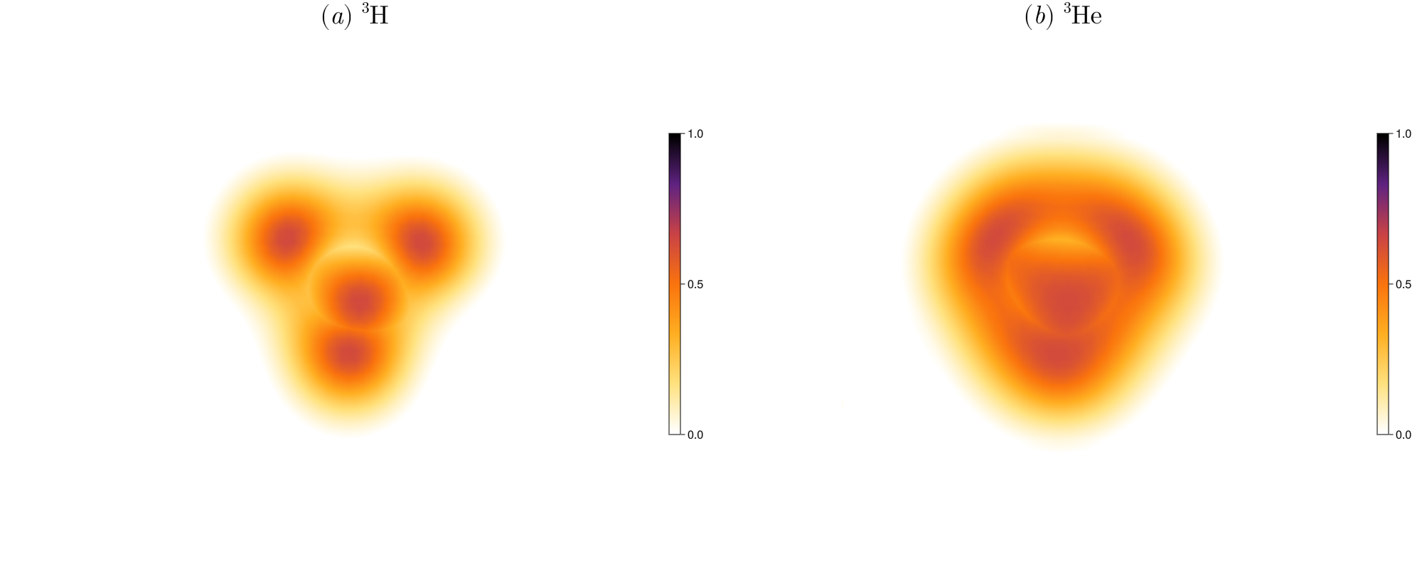
Figure 2: Charge densities of tritium and helium-3 ground states (in units of the electron charge)

IV Neutron skin thickness of Skyrmions

As we have seen, nuclei are described as classical topological solitons in the Skyrme model. By quantizing the skyrmions, we can compute an associated charge density for each quantum state. This is identified with an effective “proton density”. Following a similar argument, the neutron density is given by

$$\rho_{n}=B_{0}-\rho_{p}=\frac{1}{2}B_{0}-\expectationvalue{I_{3}^{0}}$$ (29)

so we can, in principle, compute the neutron skin thickness, $\Delta R_{np}$, of a given nucleus once we know its associated quantum state in the Skyrme model. It is given by

$$\Delta R_{np}=R_{n}-R_{p}$$ (30)

where

$$R_{n}=\frac{1}{B-Z}\int\frac{1}{2}B_{0}(x)r^{2}-\expectationvalue{I_{3}^{0}}r^{2}\,d^{3}x$$ (31)

$$R_{p}=\frac{1}{Z}\int\frac{1}{2}B_{0}(x)r^{2}+\expectationvalue{I_{3}^{0}}r^{2}\,d^{3}x\,.$$ (32)

IV.1 Example: the 3-skyrmion

As an example, consider the $B=3$ ground state $\ket{\psi}$ (26), which corresponds to the $(^{3}{\rm H},^{3}{\rm He})$ isospin doublet. We again use the fact that the state is a grand spin singlet, so $\tilde{M}_{ij}$ will vanish, and so the proton radius $R_{p}$ is given by

$$R_{p}^{2}(\psi) =\frac{1}{Z}\int\quantity[\frac{1}{2}B_{0}r^{2}+\expectationvalue{I_{3}^{0}}r^{2}]d^{3}x$$ (33)

$$=\frac{1}{Z}\quantity[\frac{1}{2}\int B_{0}r^{2}d^{3}x-\frac{M_{ij}(\psi)}{(uv-w^{2})}\quantity[(v-w)u_{ij}^{(2)}+(u-w)w_{ij}^{(2)}]],$$

where we have defined the second moment of the inertia tensors

$$u_{ij}^{(2)}\doteq\int u_{ij}(x)r^{2}d^{3}x,\qquad w_{ij}^{(2)}\doteq\int w_{ij}(x)r^{2}d^{3}x.$$ (34)

Further, by the tetrahedral symmetry of the $B=3$

$$u_{ij}^{(2)}=u^{(2)}\delta_{ij},\qquad w_{ij}^{(2)}=w^{(2)}\delta_{ij}\,,$$ (35)

which allows us to use the identities $M_{ii}=\bra{\psi}R_{3i}K_{i}\ket{\psi}=-\bra{\psi}I_{3}\ket{\psi}=-i_{3}$, which simplifies the calculation significantly. The proton density rms radius is

$$R_{p}^{2}(\psi)=\frac{1}{Z}\quantity[\frac{1}{2}B^{(2)}+\frac{(v-w)u^{(2)}+(u-w)w^{(2)}}{(uv-w^{2})}i_{3}],$$ (36)

where $B^{(2)}=Br_{rms}^{2}$, with $r_{rms}^{2}$ the rms matter radius.

Similarly, we can calculate the neutron density rms radius. It is

$$R_{n}^{2}(\psi)=\frac{1}{3-Z}\quantity[\frac{1}{2}B^{(2)}-\frac{(v-w)u^{(2)}+(u-w)w^{(2)}}{(uv-w^{2})}i_{3}].$$ (37)

Overall, we have

$$R_{p}(^{3}{\rm He})=\sqrt{\frac{1}{4}\quantity[B^{(2)}+\frac{(v-w)u^{(2)}+(u-w)w^{(2)}}{(uv-w^{2})}]}=R_{n}(^{3}{\rm H}),$$ (38)

$$R_{n}(^{3}{\rm He})=\sqrt{\frac{1}{2}\quantity[B^{(2)}-\frac{(v-w)u^{(2)}+(u-w)w^{(2)}}{(uv-w^{2})}]}=R_{p}(^{3}{\rm H}).$$ (39)

To find the neutron skin thickness of ³H, we must calculate $u,w,v,u^{(2)}$ and $w^{(2)}$. The final two quantities are quite difficult to calculate numerically. Their density scales as e.g. $u_{ij}r^{2}$. If there is an $O(\epsilon)$ error in the Skyrme field, this error is also present in the $u_{ij}$ density and the $r^{2}$ further compounds the error. To gain confidence in our numerical methods, we calculated the quantities in the rational map approximation, using the identities in Manko et al. (2007). To compare, fix the parameters $f_{\pi}=131.3\operatorname{MeV}$, $e=4.628$, and the physical value of the pion mass. The rational map skyrmion has $u_{\text{RM}}^{(2)}=770.55\text{ MeV fm}^{4}$ and $w_{\text{RM}}^{(2)}=-466.36\text{ MeV fm}^{4}$ while our full field numerics give $u^{(2)}=722.57\text{ MeV fm}^{4}$ and $w^{(2)}=-424.43\text{ MeV fm}^{4}$. Noting that the rational map skyrmions are approximations, the near agreement between calculations gives us confidence in our numerical method.

Overall, the neutron skin thickness of ³H in the Skyrme model is

$$\Delta R_{np}(^{3}{\rm H})=-R_{np}(^{3}{\rm He})\approx 0.23{\rm\,fm}.$$ (40)

The measured charge radii of ${}^{3}{\rm He}$ and ${}^{3}{\rm H}$ are $1.959\pm 0.03\operatorname{fm}$ and $1.755\pm 0.086\operatorname{fm}$, respectively Sick (2001). Assuming perfect isospin symmetry, their difference measures the NST since

$$\Delta R_{np}(^{3}{\rm H})=R_{n}(^{3}{\rm H})-R_{p}(^{3}{\rm H})=R_{p}(^{3}{\rm He})-R_{p}(^{3}{\rm H})\,,$$ (41)

giving the experimental result $\Delta R_{np}(^{3}{\rm H})\evaluated{}_{\rm exp}\approx 0.2\operatorname{fm}$. For our choice of parameters, the predicted difference in charge radii of the ${}^{3}{\rm H}-^{3}{\rm He}$ isodoublet comes out very close to the experimental value.

IV.2 Large nuclei

We now attempt to compute the NST for larger nuclei, without specific details of their quantization. The difficult part is to calculate the expectation value of $I_{3}^{0}$, given by

$$\expectationvalue{I_{3}^{0}}=-\frac{1}{2}\bra{\psi}\quantity[\frac{(u-v)u_{ab}+(u-w)w_{ab}}{(uv-w^{2})}[R_{3a}K_{b}]_{+}+\frac{wu_{ab}+uw_{ab}}{(uv-w^{2})}[R_{3a},M_{b}]_{+}]\ket{\psi}\,.$$ (42)

It is possible to evaluate this expression for generic wavefunctions if we use three approximations:

$$u_{ab}(x)=u(x)\delta_{ab},\quad|w_{ab}|\ll u,\quad u\ll v\,.$$ (43)

To check the first approximation, which we call iso-sphericity, we have calculated its accuracy for the “smorgasbord of skyrmions”, a collection of 409 skyrmion solutions with $B=1-16$ Gudnason and Halcrow (2022). We plot the percentage error of the approximation in Fig. 3, defined as

$$\text{err}=\frac{||u_{ab}-u\delta_{ab}||}{||u_{ab}||},\quad\text{with}\quad||u||^{2}=\sum_{a,b}u_{ab}u_{ba}\,.$$ (44)

The error is always below $8\%$ for $B>4$, and takes an average value of around $3\%$. Hence this seems to be a reasonable approximation to make. The mixed iso-term $w$ is generally small, and we will check the approximation numerically for the large skyrmions we create later in the paper. Generally, the spatial inertia tensor $V_{ij}$ grows as $B^{2}$ while $U_{ij}$ grows linearly with $B$. Hence we do expect the third approximation to be valid at large $B$.

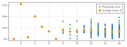
Figure 3: The percentage error in the iso-sphericity approximation $u_{ab}=u\delta_{ab}$ as a function of $B$, for the 409 skyrmion solutions found in Gudnason and Halcrow (2022).

We now apply the approximations, significantly simplifying (42) to

$$\expectationvalue{I_{3}^{0}}=-\frac{1}{2}\bra{\psi}\quantity[\frac{u(x)}{u}[R_{3a}K_{a}]_{+}]\ket{\psi}=\frac{i_{3}}{2}\frac{u(x)}{u}\,.$$ (45)

Most importantly, using the approximations means that we don’t need to know the specific structure of the ground state wavefunction $\ket{\psi}$, only its isospin value.

We can now follow the same reasoning that leads to eqs. 36 and 37, and calculate the proton and neutron rms radii for an arbitrary Skyrmion of baryon charge $B$. They are

$$R_{p}^{2}(B,i_{3})=\frac{1}{B+2i_{3}}\quantity[B^{(2)}+2\frac{u^{(2)}}{u}i_{3}]=\frac{1}{1-\delta}\quantity[r_{rms}^{2}-\frac{u^{(2)}}{u}\delta],$$ (46)

$$R_{n}^{2}(B,i_{3})=\frac{1}{B-2i_{3}}\quantity[B^{(2)}-2\frac{u^{(2)}}{u}i_{3}]=\frac{1}{1+\delta}\quantity[r_{rms}^{2}+\frac{u^{(2)}}{u}\delta],$$ (47)

where

$$\delta=-\frac{2i_{3}}{B}=\frac{N-Z}{B}$$ (48)

is the isospin asymmetry, with $N$ and $Z$ the corresponding numbers of neutrons and protons in the nucleus. Given eqs. 46 and 47, we can get a rough estimate for the NST of any nucleus from the Skyrme model, just by computing properties of the corresponding classical solution.

To understand the basic physics controlling the neutron skin, we can simplify further by assuming that $B\gg i_{3}$ (or, equivalently, $\delta\ll 1$. We insert this identity and remove a factor of $B/B$, to rearrange the radii as

$$R_{p}^{2}\approx r_{rms}^{2}-\delta\left(\frac{u^{(2)}}{u}-r_{rms}^{2}\right)\implies R_{p}\approx r_{rms}\quantity[1-\frac{\delta}{2}\quantity(\frac{u^{(2)}}{r_{rms}^{2}u}-1)].$$ (49)

Hence the NST is given by

$$\Delta R_{np}\approx\delta\,\left(\frac{u^{(2)}}{ur^{2}_{rms}}-1\right)r_{rms}\,.$$ (50)

The quantity $u^{(2)}/u$ measures the root-mean-squared radius associated to the isospin density. Hence, the sign and magnitude of the neutron skin depends on the difference between the matter and isospin charge radii, $u^{(2)}/u-r^{2}_{rms}$.

Experimentally, the NST is measured to depend linearly on the isospin asymmetry, with a slope that seems to be independent of the baryon number in the range $16<B<238$ (see fig. 2 in Novario et al. (2023)) and parametrized by

$$\Delta R_{np}=1.32\,\delta-0.024\pm 0.026\,{\rm fm}.$$ (51)

In the next Section, we test if this linear behavior is reproduced for the Skyrme model. The relationship between $\Delta R_{np}$ and $\delta$ is expected to become nonlinear for small nuclei, in which few body interactions may dominate over bulk effects Novario et al. (2023). It is precisely in this range of the baryon charge where the solutions of the Skyrme model have been extensively studied, including a recent exhaustive description of the landscape of all known local minima in the Skyrmion configuration space up to $B=16$ Gudnason and Halcrow (2022).

V Numerical Results

Unfortunately, both the computational time required to find a minimum and the number of such local minima tend to grow very rapidly with the baryon number of the configurations, which makes it computationally very demanding to perform a systematic study of very large $(B\sim 100)$ Skyrmions. Nevertheless, we have been able to generate new classical solutions for Skyrmions with $B$ up to $256$ using the Skyrmions3D.jl package Halcrow (2023), which allows one to create and visualize 3D Skyrmions in the Skyrme model of nuclear matter, and compute their properties such as energy, baryon number, moments of inertia and the corresponding densities, etc. We have generated Skyrmions constructed from $B=4$ cubes, with $B=32,48,64,108,144,180,196,240$ and $256$. Each skyrmion is made on a cubic lattice with spacing $0.2$. The size of the lattice is adjusted depending on the size of the skyrmion. The largest lattice used was $160^{3}$ for the $B=256$ skyrmion; this is the largest-$B$ skyrmion ever created. We used Neumann boundary conditions and an arrested Newton Flow Battye and Sutcliffe (2002). The flow is stopped when the maximum absolute value of the variation at any lattice point is less than $0.01$.

We first test the three approximations, listed in (43), for our numerically generated skyrmions. The percentage error in the sphericity approximation $u_{ab}=u\delta_{ab}$, the value $\text{max}_{a,b}(|w_{ab}|/u)$ and the value $u/v$ are plotted in Figure 4. All these should be much less than one for our method to be accurate. Overall, the results are reassuring. The least accurate assumption is the iso-sphericity approximation, which has a $\sim 10\%$ error.

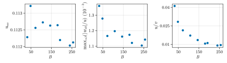
Figure 4: The percentage error in the iso-sphericity approximation $u_{ab}=u\delta_{ab}$, the value $\text{max}_{a,b}(|w_{ab}|/u)$ and the value $u/v$ for the numerically generated large skyrmions.

Using the numerically generated solutions, we can compute the NST of these large $B$ configurations and compare them to the experimental results. To do so, we calculate $\left(u^{(2)}/ur^{2}_{rms}-1\right)r_{rms}$ for the numerically generated Skyrmions. We plot these results, and energy densities of the generated skyrmion, in Fig. 5. Remarkably, the value changes little over this large range of baryon numbers. From $B=64$ to $B=240$, the values change by around $10\%$. There is a clear decrease as $B$ increases, but the leading order behavior is constant. Hence the Skyrme model reproduces the linear relationship between $\Delta R_{np}$ and $\delta$. We then predict a correction, inversely proportional to $B$.

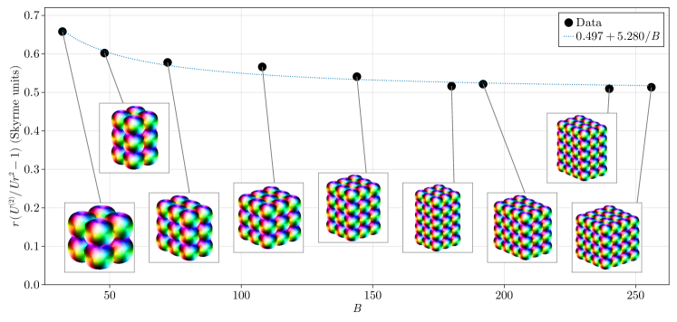
Figure 5: $r(U^{(2)}/Ur^{2}-1)$ in Skyrme units as a function of the baryon number, for $m=0.2$.

Our results depend on our calibration and hence on the pion mass $m$. To check this dependence, we calculate $\left(u^{(2)}/ur^{2}_{rms}-1\right)r_{rms}$ for a variety of $m$. To leading order, the important quantity is the constant part of this. We calculate it by taking the average over $B=108-265$. To calibrate the model, we must set the length scale of the Skyrme model which in turn sets the dimensionless pion mass, $m$. We will fix the length scale by comparing the baryon rms radius of the $B=108$ Skyrmion, $r_{108}$ to the radius of Tin-50 $r_{\text{Sn}}$ (Note: this calibration ensures the radii of all large nuclei are reasonably well described in a rigid rotor approximation). So in physical units, our result is

$$\frac{\Delta R_{np}}{\delta}=\frac{r_{\rm Sn}r_{rms}}{r_{108}}\left(\frac{u^{(2)}}{ur^{2}_{rms}}-1\right)\,\text{fm}\,.$$ (52)

This is a function of the parameter $m$, which we can fit to match the linear relationship (51). We plot (52) as a function of $m$ in Fig. 6. The result is highly sensitive to $m$. The value of $m$ which gives the best fit is $m=0.0$, giving

$$\Delta R_{np}=0.92\delta$$ (53)

This is to be compared to the result from experiments $\Delta R_{np}=1.32\delta$ Novario et al. (2023), and the liquid drop model $\Delta R_{np}=0.75\delta$ Pethick and Ravenhall (1996).

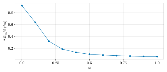
Figure 6: The average $\Delta R_{np}/\delta$ in $\operatorname{fm}$, as a function of the dimensionless pion mass parameter $m$.

Unfortunately, $m$ is not really a free parameter. It is related to the physical pion mass $m_{\pi}$. If we take $m_{\pi}$ equal to its physical value, $138$ MeV, we find that $m\approx 0.5$ and so $\Delta R_{np}=0.15\delta$. This is too small by an order of magnitude. That the pion mass, which should provide a small correction in chiral effective field theories, makes such a large difference is surprising.

VI Relation to the Symmetry Energy

The nuclear symmetry energy $S(n)$ is defined as the difference between the energy (per baryon number) of infinite, pure neutron matter and isospin symmetric nuclear matter at a given baryon density $n$. Although its dependence on the density has proven difficult to measure experimentally, it is usually parametrized as an expansion in powers of the baryon density around nuclear saturation $n_{0}\approx 0.16\operatorname{fm}$,

$$S_{N}(n_{B})=S_{0}+\frac{1}{3}L\epsilon+\frac{1}{18}K_{\rm sym}\epsilon^{2}+\cdots$$ (54)

with $\epsilon=(n-n_{0})/n_{0}$, and

$$L=3n_{0}\partialderivative{S_{N}}{n}\evaluated{}_{n=n_{0}},\quad K_{\rm sym}=9n_{0}^{2}\partialderivative[2]{S_{N}}{n}\evaluated{}_{n=n_{0}}$$ (55)

the slope and curvature of the symmetry energy at saturation, respectively. The symmetry energy at saturation is well constrained ($S_{0}\sim 30$ MeV) by nuclear experiments, but the values of the slope and higher order coefficients are still very uncertain (see e.g. the recent review Lattimer (2023)).

The existence of a strong, model-independent correlation between the neutron skin thicknesses of neutron-rich nuclei, such as ${}^{48}{\rm Ca}$ and ${}^{208}{\rm Pb}$, and the symmetry energy slope parameter $L$ has been well established both from the experimental and theoretical ends Lattimer (2023); Sammarruca (2023). Indeed, the symmetry energy slope can be understood as a pressure gradient acting on excess neutrons, which determines the formation and size of the neutron skin. Therefore, measurements of the neutron skin of nuclei can provide constraints on $L$, and hence on the nuclear matter equation of state.

In the Skyrme model, infinite nuclear matter can be described as a periodic crystal of half-skyrmions with cubic unit cells Klebanov (1985). The symmetry energy of such crystals can be obtained in the rigid rotor approximation, which yields a simple expression in terms of the isospin moment of inertia of the unit cell $\Lambda$ Adam et al. (2022a):

$$S(n)=\frac{\hbar^{2}}{2\Lambda}.$$ (56)

As with finite nuclei, the computation of the isospin inertia moment must be done numerically for each value of the unit cell length parameter $l$. Hence, there is not an analytic expression for $\Lambda(l)$. However, it was shown in Adam et al. (2022b) that the crystal displays an almost perfect scaling property with $l$. This property means that each of the terms in the energy functional (8) scales with $l$ independently as $E_{i}\propto l^{-i+3}$, where $i$ is the number of spatial derivatives appearing in that particular term. This perfect scaling property is a characteristic of the field configuration and not only of its energy. Indeed, it is observed also for the isospin moment of inertia of the crystal Adam et al. (2023). Hence the (adimensional) energy $E$ and isospin moment of inertia $\Lambda$ of the cubic unit cell approximately satisfy the following expressions,

$$E(l,m) =K_{2}l+\frac{K_{4}}{l}+m^{2}K_{0}l^{3},$$ (57)

$$\Lambda(l) =\Lambda_{2}l^{3}+\Lambda_{4}l,$$ (58)

where the values of $K_{i}$ and $\Lambda_{i}$ are “universal”, i.e., they do not depend on either the parameters or $l$. The values of these universal scaling constants have been obtained in Adam et al. (2023) and are given by

$$K_{0}=0.017,\quad K_{2}= 0.466,\quad K_{4}=9.617,$$ (59)

$$\Lambda_{2}=0.038, \quad\Lambda_{4}=1.393.$$ (60)

The above values are dimensionless, but were obtained using a different convention of Skyrme units. As we will be mainly interested in the behavior of $L$ with the pion mass parameter, and not on its specific value, we may as well use them.

Although the scaling is not perfect, in general the largest deviations from the true numerical values of energy start quite far from the minimum, at which the perfect scaling fit is most precise. Taking advantage of this almost perfect scaling property, we can write the symmetry energy slope at saturation as

$$L=3n_{0}\partialderivative{S}{n}\evaluated{}_{n_{0}}\equiv\frac{\hbar^{2}}{2}\frac{\Lambda^{\prime}(l_{0})}{\Lambda^{2}(l_{0})}l_{0}$$ (61)

where $l_{0}$ is the unit cell length at saturation, i.e. at the minimum of $E(l,m)$ for any given $m$:

$$\partialderivative{E(l,m)}{l}\evaluated{}_{l_{0}}=0\implies l_{0}=\sqrt{\frac{\sqrt{K_{2}^{2}+12m^{2}K_{0}K_{4}}-K_{2}}{6m^{2}K_{0}}}.$$ (62)

Equations (61) and (62) above implicitly define a function $L(m)$, so we can study the correlation between the NST $\Delta R_{np}$ and the symmetry energy slope at saturation $L$ in the Skyrme model by comparing how they change with the pion mass parameter $m$.

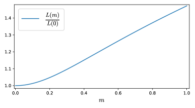
Figure 7: Symmetry energy slope as a function of the pion mass parameter in the Skyrme model.

In fig. 7 we show the dependence of the symmetry energy slope $L$ with the pion mass parameter. Surprisingly, comparing with fig. 6, we find that the symmetry energy slope and the neutron skin thickness are anti-correlated: while $L$ grows with increasing $m$, the NST decreases. This is precisely opposite to what was a priori expected from other nuclear models and constitutes a very unique feature of the Skyrme model.

VII Conclusions

Overall, in the Skyrme model, the neutron skin thickness is proportional to the isospin asymmetry, with a constant of proportionality equal to the difference between matter and isospin charge radii (multiplied by the matter radius). This quantity has a weak dependence on baryon number, thus approximately reproduces the linear relationship seen in experimental data. Importantly, thanks to several approximations, we can derive almost everything analytically and find an expression for the neutron-skin thickness with a simple physical interpretation. This is a key advantage of the Skyrme model: using it, we can make analytical progress on difficult problems.

Using the physical pion mass, the constant of proportionality was much too small. This can be improved by decreasing the physical pion mass. There are several ways to interpret the result. The pion mass may be renormalized for large skyrmions, so a value different than the physical mass is reasonable to choose. Another possibility is that our calculation has only captured one contribution to the total neutron skin thickness, due to the simplicity of the original Skyrme model. A natural extension of the results presented here would be to include further interaction terms and/or degrees of freedom, which will affect the classical skyrmion solutions. For instance, vector mesons Fujiwara et al. (1985), or the sixth order term in $L_{\mu}$, first proposed in Jackson et al. (1985) (see also Adkins and Nappi (1984)), which can be seen as an effective point-like interaction that describes the repulsive exchange of omega vector mesons. The latter term has been shown to become relevant at sufficiently high densities (i.e. may be important to model large nuclei such as the ones we have been working with in this paper) and be crucial for an accurate description of the high-density equation of state of neutron stars Adam et al. (2020, 2022c). A final possibility is that we may have excluded an important theoretical consideration such as the Coulomb forces, which may alter the shape of large skyrmions and modify the final result.

References

References

- Hofstadter (1956) Robert Hofstadter, “Electron scattering and nuclear structure,” Rev. Mod. Phys. 28, 214–254 (1956).
- De Jager et al. (1974) C. W. De Jager, H. De Vries, and C. De Vries, “Nuclear charge and magnetization density distribution parameters from elastic electron scattering,” Atom. Data Nucl. Data Tabl. 14, 479–508 (1974), [Erratum: Atom.Data Nucl.Data Tabl. 16, 580–580 (1975)].
- Perdrisat et al. (2007) C. F. Perdrisat, V. Punjabi, and M. Vanderhaeghen, “Nucleon Electromagnetic Form Factors,” Prog. Part. Nucl. Phys. 59, 694–764 (2007), arXiv:hep-ph/0612014 .
- Punjabi et al. (2015) V. Punjabi, C. F. Perdrisat, M. K. Jones, E. J. Brash, and C. E. Carlson, “The Structure of the Nucleon: Elastic Electromagnetic Form Factors,” Eur. Phys. J. A 51, 79 (2015), arXiv:1503.01452 [nucl-ex] .
- Camsonne et al. (2014) A. Camsonne et al. (The Jefferson Lab Hall A Collaboration), “Jlab measurement of the charge form factor at large momentum transfers,” Phys. Rev. Lett. 112, 132503 (2014).
- Arrington et al. (2023) John Arrington, Reynier Cruz-Torres, Tyler J. Hague, Leiqaa Kurbany, Shujie Li, David Meekins, and Nathaly Santiesteban, “The Jefferson Lab tritium program of nucleon and nuclear structure measurements,” (2023), arXiv:2304.09998 [nucl-ex] .
- Sachs (1962) R. G. Sachs, “High-energy behavior of nucleon electromagnetic form factors,” Phys. Rev. 126, 2256–2260 (1962).
- Lorcé (2020) Cédric Lorcé, “Charge distributions of moving nucleons,” Phys. Rev. Lett. 125, 232002 (2020), arXiv:2007.05318 [hep-ph] .
- Miller (2007) Gerald A. Miller, “Charge Density of the Neutron,” Phys. Rev. Lett. 99, 112001 (2007), arXiv:0705.2409 [nucl-th] .
- Jaffe (2021) Robert L. Jaffe, “Ambiguities in the definition of local spatial densities in light hadrons,” Phys. Rev. D 103, 016017 (2021), arXiv:2010.15887 [hep-ph] .
- Epelbaum et al. (2022) E. Epelbaum, J. Gegelia, N. Lange, U. G. Meißner, and M. V. Polyakov, “Definition of Local Spatial Densities in Hadrons,” Phys. Rev. Lett. 129, 012001 (2022), arXiv:2201.02565 [hep-ph] .
- Gao and Vanderhaeghen (2022) Haiyan Gao and Marc Vanderhaeghen, “The proton charge radius,” Rev. Mod. Phys. 94, 015002 (2022), arXiv:2105.00571 [hep-ph] .
- Polyakov and Schweitzer (2018) Maxim V. Polyakov and Peter Schweitzer, “Forces inside hadrons: pressure, surface tension, mechanical radius, and all that,” Int. J. Mod. Phys. A 33, 1830025 (2018), arXiv:1805.06596 [hep-ph] .
- Krasznahorkay et al. (2004) A. Krasznahorkay, H. Akimune, A.M. van den Berg, N. Blasi, S. Brandenburg, M. Csatlo´s, M. Fujiwara, J. Gulya´s, M.N. Harakeh, M. Hunyadi, M. de Huu, Z. Ma´te, D. Sohler, S.Y. van der Werf, H.J. Wo¨rtche, and L. Zolnai, “Neutron-skin thickness in neutron-rich isotopes,” Nuclear Physics A 731, 224–234 (2004).
- Xu (2023) Haojie Xu (STAR), “Constraints on Neutron Skin Thickness and Nuclear Deformations Using Relativistic Heavy-ion Collisions from STAR,” Acta Phys. Polon. Supp. 16, 1–A30 (2023), arXiv:2208.06149 [nucl-ex] .
- Li et al. (2020) Hanlin Li, Hao-jie Xu, Ying Zhou, Xiaobao Wang, Jie Zhao, Lie-Wen Chen, and Fuqiang Wang, “Probing the neutron skin with ultrarelativistic isobaric collisions,” Phys. Rev. Lett. 125, 222301 (2020).
- Mondal et al. (2016) C. Mondal, B. K. Agrawal, M. Centelles, G. Colò, X. Roca-Maza, N. Paar, X. Viñas, S. K. Singh, and S. K. Patra, “Model dependence of the neutron-skin thickness on the symmetry energy,” Phys. Rev. C 93, 064303 (2016), arXiv:1605.05048 [nucl-th] .
- Lattimer (2023) James M. Lattimer, “Constraints on Nuclear Symmetry Energy Parameters,” Particles 6, 30–56 (2023), arXiv:2301.03666 [nucl-th] .
- Sammarruca (2023) Francesca Sammarruca, “The neutron skin of 48Ca and 208Pb: a critical analysis,” (2023), arXiv:2311.02539 [nucl-th] .
- Adhikari et al. (2021) D. Adhikari et al. (PREX Collaboration), “Accurate determination of the neutron skin thickness of through parity-violation in electron scattering,” Phys. Rev. Lett. 126, 172502 (2021).
- Adhikari et al. (2022) D. Adhikari et al. (CREX Collaboration), “Precision determination of the neutral weak form factor of ,” Phys. Rev. Lett. 129, 042501 (2022).
- Horowitz et al. (2001) C. J. Horowitz, S. J. Pollock, P. A. Souder, and R. Michaels, “Parity violating measurements of neutron densities,” Phys. Rev. C 63, 025501 (2001), arXiv:nucl-th/9912038 .
- Roca-Maza et al. (2011) X. Roca-Maza, M. Centelles, X. Vinas, and M. Warda, “Neutron skin of , nuclear symmetry energy, and the parity radius experiment,” Phys. Rev. Lett. 106, 252501 (2011), arXiv:1103.1762 [nucl-th] .
- Freedman (1974) Daniel Z. Freedman, “Coherent Neutrino Nucleus Scattering as a Probe of the Weak Neutral Current,” Phys. Rev. D 9, 1389–1392 (1974).
- Patton et al. (2012) Kelly Patton, Jonathan Engel, Gail C. McLaughlin, and Nicolas Schunck, “Neutrino-nucleus coherent scattering as a probe of neutron density distributions,” Phys. Rev. C 86, 024612 (2012), arXiv:1207.0693 [nucl-th] .
- Payne et al. (2019) C. G. Payne, S. Bacca, G. Hagen, W. Jiang, and T. Papenbrock, “Coherent elastic neutrino-nucleus scattering on 40Ar from first principles,” Phys. Rev. C 100, 061304 (2019), arXiv:1908.09739 [nucl-th] .
- Akimov et al. (2017) D. Akimov et al. (COHERENT), “Observation of Coherent Elastic Neutrino-Nucleus Scattering,” Science 357, 1123–1126 (2017), arXiv:1708.01294 [nucl-ex] .
- Akimov et al. (2021) D. Akimov et al. (COHERENT), “First Measurement of Coherent Elastic Neutrino-Nucleus Scattering on Argon,” Phys. Rev. Lett. 126, 012002 (2021), arXiv:2003.10630 [nucl-ex] .
- Braaten and Carson (1989) Eric Braaten and Larry Carson, “The Deuteron as a Toroidal Skyrmion: Electromagnetic Form-factors,” Phys. Rev. D 39, 838 (1989).
- Carson (1991a) Larry Carson, “Static properties of He-3 and H-3 in the Skyrme model,” Nucl. Phys. A 535, 479–496 (1991a).
- Karliner et al. (2016) M. Karliner, C. King, and N. S. Manton, “Electron Scattering Intensities and Patterson Functions of Skyrmions,” J. Phys. G 43, 055104 (2016), arXiv:1510.00280 [nucl-th] .
- Garcia Martin-Caro et al. (2023) Alberto Garcia Martin-Caro, Miguel Huidobro, and Yoshitaka Hatta, “Gravitational form factors of nuclei in the Skyrme model,” Phys. Rev. D 108, 034014 (2023), arXiv:2304.05994 [nucl-th] .
- Adkins et al. (1983) Gregory S. Adkins, Chiara R. Nappi, and Edward Witten, “Static Properties of Nucleons in the Skyrme Model,” Nucl. Phys. B 228, 552 (1983).
- Braaten et al. (1986) Eric Braaten, Sze-Man Tse, and Charles Willcox, “Electroweak form factors of the skyrmion,” Phys. Rev. D 34, 1482–1492 (1986).
- Manko et al. (2007) Olga V. Manko, Nicholas S. Manton, and Stephen W. Wood, “Light nuclei as quantized skyrmions,” Phys. Rev. C 76, 055203 (2007), arXiv:0707.0868 [hep-th] .
- Carson (1991b) Larry Carson, “B = 3 nuclei as quantized multiskyrmions,” Phys. Rev. Lett. 66, 1406–1409 (1991b).
- Sick (2001) I. Sick, “Elastic electron scattering from light nuclei,” Progress in Particle and Nuclear Physics 47, 245–318 (2001).
- Gudnason and Halcrow (2022) Sven Bjarke Gudnason and Chris Halcrow, “A Smörgåsbord of Skyrmions,” JHEP 08, 117 (2022), arXiv:2202.01792 [hep-th] .
- Novario et al. (2023) S. J. Novario, D. Lonardoni, S. Gandolfi, and G. Hagen, “Trends of Neutron Skins and Radii of Mirror Nuclei from First Principles,” Phys. Rev. Lett. 130, 032501 (2023), arXiv:2111.12775 [nucl-th] .
- Halcrow (2023) C. Halcrow, “Skyrmions3D,” https://github.com/chrishalcrow/Skyrmions3D.jl (2023).
- Battye and Sutcliffe (2002) Richard A. Battye and Paul M. Sutcliffe, “Skyrmions, fullerenes and rational maps,” Rev. Math. Phys. 14, 29–86 (2002), arXiv:hep-th/0103026 .
- Pethick and Ravenhall (1996) CJ Pethick and DG Ravenhall, “The dependence of neutron skin thickness and surface tension on neutron excess,” Nuclear Physics A 606, 173–182 (1996).
- Klebanov (1985) Igor R. Klebanov, “Nuclear Matter in the Skyrme Model,” Nucl. Phys. B 262, 133–143 (1985).
- Adam et al. (2022a) Christoph Adam, Alberto García Martín-Caro, Miguel Huidobro, Ricardo Vázquez, and Andrzej Wereszczynski, “Quantum skyrmion crystals and the symmetry energy of dense matter,” Phys. Rev. D 106, 114031 (2022a), arXiv:2202.00953 [nucl-th] .
- Adam et al. (2022b) Christoph Adam, Alberto Garcia Martin-Caro, Miguel Huidobro, Ricardo Vazquez, and Andrzej Wereszczynski, “Dense matter equation of state and phase transitions from a generalized Skyrme model,” Phys. Rev. D 105, 074019 (2022b), arXiv:2109.13946 [hep-th] .
- Adam et al. (2023) Christoph Adam, Alberto Garcia Martin-Caro, Miguel Huidobro, and Andrzej Wereszczynski, “Skyrme Crystals, Nuclear Matter and Compact Stars,” Symmetry 15, 899 (2023), arXiv:2305.06639 [nucl-th] .
- Fujiwara et al. (1985) T. Fujiwara, Y. Igarashi, A. Kobayashi, H. Otsu, T. Sato, and S. Sawada, “An Effective Lagrangian for Pions, Mesons and Skyrmions,” Prog. Theor. Phys. 74, 128 (1985).
- Jackson et al. (1985) A. Jackson, A. D. Jackson, A. S. Goldhaber, G. E. Brown, and L. C. Castillejo, “A MODIFIED SKYRMION,” Phys. Lett. B 154, 101–106 (1985).
- Adkins and Nappi (1984) Gregory S. Adkins and Chiara R. Nappi, “Stabilization of Chiral Solitons via Vector Mesons,” Phys. Lett. B 137, 251–256 (1984).
- Adam et al. (2020) Christoph Adam, Alberto García Martín-Caro, Miguel Huidobro, Ricardo Vázquez, and Andrzej Wereszczynski, “A new consistent neutron star equation of state from a generalized Skyrme model,” Phys. Lett. B 811, 135928 (2020), arXiv:2006.07983 [hep-th] .
- Adam et al. (2022c) Christoph Adam, Alberto García Martín-Caro, Miguel Huidobro, Ricardo Vázquez, and Andrzej Wereszczynski, “Kaon condensation in skyrmion matter and compact stars,” (2022c), arXiv:2212.00385 [nucl-th] .
- Bjarke Gudnason and Halcrow (2018) Sven Bjarke Gudnason and Chris Halcrow, “Vibrational modes of Skyrmions,” Phys. Rev. D 98, 125010 (2018), arXiv:1811.00562 [hep-th] .