Polarimetric Light Transport Analysis
for Specular Inter-reflection

Abstract

Polarization is well known for its ability to decompose diffuse and specular reflections. However, the existing decomposition methods only focus on direct reflection and overlook multiple reflections, especially specular inter-reflection. In this paper, we propose a novel decomposition method for handling specular inter-reflection of metal objects by using a unique polarimetric feature: the rotation direction of linear polarization. This rotation direction serves as a discriminative factor between direct and inter-reflection on specular surfaces. To decompose the reflectance components, we actively rotate the linear polarization of incident light and analyze the rotation direction of the reflected light. We evaluate our method using both synthetic and real data, demonstrating its effectiveness in decomposing specular inter-reflections of metal objects. Furthermore, we demonstrate that our method can be combined with other decomposition methods for a detailed analysis of light transport. As a practical application, we show its effectiveness in improving the accuracy of 3D measurement against strong specular inter-reflection.

I Introduction

The analysis of light transport is an important task in computer vision, allowing us to understand the real-world scene through various optical phenomena, such as diffuse and specular reflection, subsurface scattering, and inter-reflection. These phenomena repeatedly occur in intricate geometry and materials, resulting in a complex mixture of light observations. Sometimes, these mixed lights lead to difficulties in subsequent tasks, such as 3D measurement and material classification. Therefore, analyzing the mixed light transport is essential for understanding the scene.

There are numerous different techniques to decompose light transport components. These techniques use the relationship between reflection components and optical properties, such as the dichromatic reflectance model [1, 2, 3, 4, 5, 6], spatial frequency response [7], geometric constraint [8, 9, 10], far infrared light [11] and polarization [12, 13, 14, 15, 16, 17, 18]. Our polarization-based method falls within that category.

Polarization is a renowned physical cue to decompose diffuse and specular reflection components. Numerous polarization-based methods exploit the behavior of reflection, wherein a diffuse surface makes the incident light unpolarized while a specular surface preserves its polarization [12, 13, 14, 15, 16, 17, 18]. These methods assume that all indirect reflection components are unpolarized, similar to diffuse surface reflection or subsurface scattering. However, this assumption is not always true because inter-reflection on specular surfaces preserves the polarization of the incident light. Therefore, the existing methods are not capable of explicitly handling specular inter-reflection.

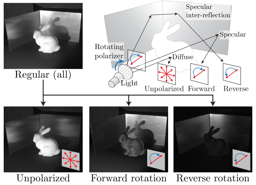
Figure 1: Overview of reflectance components decomposition based on the rotation of linear polarization. Our method can decompose polarization states of the reflected light into three components: Unpolarized, Forward rotation, and Reverse rotation.

In this paper, we propose a novel polarization-based light transport decomposition method, especially for specular inter-reflection. Our method is based on the observation of specular inter-reflection that, when the polarization plane of incident light rotates, the polarization plane of the reflected light rotates in the opposite direction. We exploit this observation as a useful cue to decompose mixed light. To capture the rotation of polarization, we use a pair of linear polarizers in front of the light source and camera, and the camera captures the polarization state of the reflected light by rotating both polarizers. As shown in Fig. 1, we decompose the reflected light into three components: Unpolarized, Forward rotation, Reverse rotation. These components correspond to the diffuse reflection, specular reflection, and specular inter-reflection, respectively.

To summarize, our main contributions are:

• We present a novel polarization-based light transport decomposition method, especially for specular inter-reflection (Fig. 6), which is challenging in previous methods (Fig. 7).

• We show that our method can be combined with existing methods that use a different physical cue because our method only relies on polarization (Fig. 8).

• We show a practical application of our method: 3D measurement with a projector-camera system for metal objects (Fig. 9). With our method, we can measure the 3D shape in the presence of specular inter-reflection.

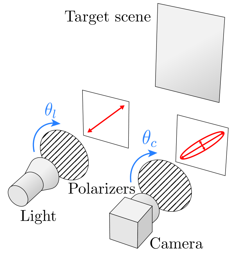
(a) Capturing configuration

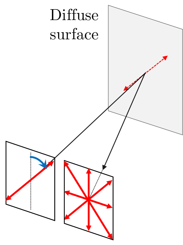
(b) Unpolarized

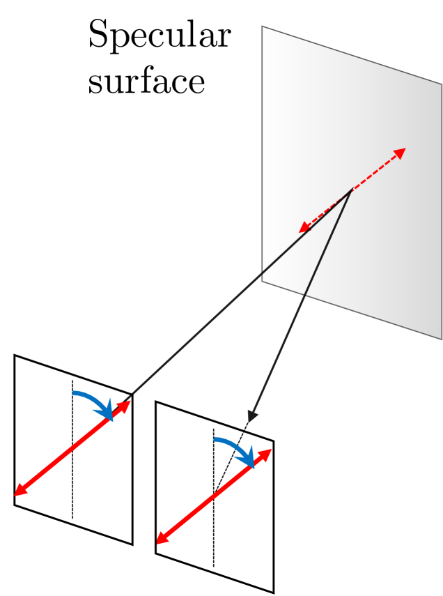
(c) Forward rotation

(d) Reverse rotation

Figure 2: Polarization states of reflected light relative to incident light’s polarization plane rotation. (a) We illuminate the target scene with a light source with a polarizer and capture the reflected light with a camera with a polarizer. (b) In diffuse reflection or subsurface scattering, the reflected light is mostly unpolarized. (c) In direct specular reflection, the polarization plane of the reflected light rotates in the same direction as the incident light. (d) In specular inter-reflection, on the other hand, the polarization plane of the reflected light rotates in the opposite direction from the incident light.

II Related Work

II-A Reflection and Light Transport Analysis

The decomposition of reflection components is an essential task for computer vision and graphics, so many researchers have explored various methods. In essence, these methods exploit the relationship between reflection components and physical optical phenomena. Shafer et al.  [1] separate diffuse and specular reflection based on the dichromatic reflectance model. This model incorporates the color difference due to diffuse and specular reflection. Several reflection decomposition methods utilize the spatially high-frequency light pattern. Nayar et al.  [7] proposed a high-frequency spatial patterns method to separate direct and global components. This principle is applied to robust 3D scanning methods against inter-reflection and subsurface scattering [19, 20, 21]. Some methods exploit the geometric constraints of the camera and light source. O’Toole et al. proposed primal-dual coding [8] using a coaxial projector-camera setup, and his follow-up work uses epipolar constraints [9, 10]. Other methods decompose reflection components by far infrared light [11] or the time-of-flight approach [22].

Polarization is also an essential cue for the decomposition of reflection. It is well known that the degree of polarization differs in diffuse and specular reflection components. Several methods have been developed to analyze the polarization states of reflected light [12, 13, 14, 17, 18], and estimate the 3D shape of translucent objects, which causes subsurface scattering [23]. There are still few studies on analyzing specular inter-reflection using polarized light. Wallance et al. distinguish direct and inter-reflection of metallic objects  [24]. However, they worked not to decompose but just distinguish them. In addition, their experimental results showed only handling horizontal inter-reflections and did not account for inter-reflections in arbitrary directions. In contrast, we decompose the reflection components, which can apply to various inter-reflection directions.

II-B Polarization in Computer Vision

In computer vision, polarization has been exploited not only for the separation of diffuse and specular reflection but also for various imaging techniques such as 3D shape recovery for both opaque [25, 26, 27] and transparent [28] objects, dehazing [15, 29], and segmentation for transparent objects [30]. These studies were conducted under uncontrollable environment light or known light sources with fixed polarizers.

Recently, Baek et al. explored the polarimetric relationship between the incident and reflected light for various imaging applications [31, 32, 33, 34]. Similar to his series of works, we measure the polarimetric information using rotating polarizers attached to both light source and camera sides. In particular, Baek and Heide briefly showed a measured result of the specular inter-reflection [33], which implies the circular polarization change in specular inter-reflection. Our research delves deeper into this polarization change by explicitly defining the mathematical model and utilizing it for decomposing light transport with polarization cue alone.

III Principle

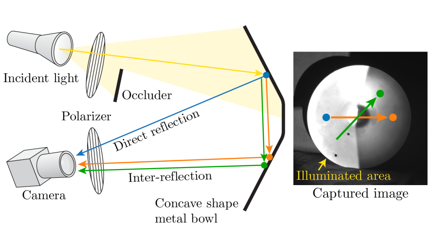
(a) Capturing setup with an occluder

(b) The polarizer angle and measured AoLP

Figure 3: Rotation of the angle of linear polarization in specular inter-reflection. This measurement focuses on three different types of reflections: direct reflection, inter-reflection (horizontal), and inter-reflection (oblique). (a) The light source illuminates the concave-shaped metal bowl with the polarized light source. The occluder blocks the light, and the bowl is illuminated only on one side. The camera observes unmixed direct reflection and inter-reflection separately. (b) The plotted result of the AoLP of reflected light $\phi$ and the polarizer angle of light side $\theta_{l}$. We can see the different trends between direct and inter-reflection ([A] and [B]) and the phase difference between horizontal and oblique inter-reflection ([C]).

In this section, we introduce the essential polarization phenomenon in specular inter-reflection that forms the cornerstone of this study. Fig. 2 illustrates three polarization states that aim to decompose, and Fig. 3 shows the actual measurement of this phenomenon. As listed below, we explain polarization states in specular inter-reflection by referring to the intuitive interpretation in Fig. 2 and the actual data in Fig. 3.

1. Degree of linear polarization. As shown in Fig. 2(b), the reflected light becomes unpolarized in diffuse reflection or subsurface scattering. In contrast, as illustrated in Fig. 2(c) and (d), polarization is preserved in specular reflection.

2. Rotation direction. As shown in Fig. 2(c), in single bounce specular reflection, the polarization planes of the incident and reflected light rotate in the same direction. On the other hand, in the case of the second bounce reflection, the rotation is reversed, as shown in Fig. 2(d). We can see this opposite trend between direct and inter-reflection, as indicated in [A] and [B] in Fig. 3(b). With respect to the polarizer angle of the incident light, the angle of linear polarization (AoLP) of the direct reflection is linearly increasing, and the inter-reflection is decreasing.

3. Phase difference. We can see the difference in phase between horizontal and oblique inter-reflection as indicated in [C] of Fig. 3(b). This phase difference depends on the light path.

We can use the difference in rotation direction as a cue to distinguish three classes of reflection as shown in Fig. 2(b)(c)(d). However, in general, we observe not a single component but a mixture of them. Therefore, in the next section, we propose the decomposition method using a mathematical model of these three components.

IV Method

In this section, we introduce our proposed decomposition method. In subsection A, we describe the basic relationship between observed intensity and polarization. Then, in subsection B, we formulate the mathematical model of three reflection components by incorporating the rotation direction of the plane of polarization. In subsection C, we show the decomposition method for three components. Finally, in subsection D, we discuss the minimum number of measurements required to apply the decomposition.

IV-A Basic Observation of Polarization

Before diving into our method, we briefly review the background of polarization. Although our proposed method uses a pair of linear polarizers in front of a light source and a camera side, we start with a single polarizer case. Suppose we measure the intensity of light with a camera that has a linear polarizer attached to the front. The camera measures the intensity $I(\theta_{c})$ at the angle of the linear polarizer $\theta_{c}$ which expressed as

$$I_{\rho,\phi}(\theta_{c})=\frac{I_{\mathrm{amp}}}{2}\{\rho\cos{2(\theta_{c}-\phi)+1}\},$$ (1)

where $I_{\mathrm{amp}}$, $\rho$, and $\phi$ are the parameters that characterize the polarization of its light. $I_{\mathrm{amp}}$ is the intensity, $\rho$ is the degree of linear polarization (DoLP), and $\phi$ is the angle of linear polarization (AoLP). The DoLP represents how much the light is polarized with a value of $1$ indicating perfectly linear polarized light and $0$ indicating unpolarized light. The AoLP represents the angle of the plane of polarization light.

The equation above only represents the case of a single polarizer of a camera. In the next subsection, we will add a polarizer to the light source and extend the equation to consider the rotation direction of the polarization plane.

IV-B Rotation Direction of Linear Polarization

We extend the basic polarization expression Eq. 1 by incorporating the rotation direction of the plane of polarization. Our method defines the three types of polarization states illustrated in Fig. 2. As shown in Fig. 2(a), the scene is illuminated by a light source with a linear polarizer and captured by a camera with a linear polarizer. Both polarizers are to be rotated independently, and the camera observes the intensity $I(\theta_{c},\theta_{l})$ at the angle of linear polarizers $\theta_{c}$ (camera side), $\theta_{l}$ (light source side). Then, we define the observed intensity as a mixture of three components,

$$I(\theta_{c},\theta_{l})=I_{\textrm{unpolarized}}(\theta_{c},\theta_{l})+I_{\textrm{forward}}(\theta_{c},\theta_{l})+I_{\textrm{reverse}}(\theta_{c},\theta_{l}),$$ (2)

where $I_{\textrm{unpolarized}}$, $I_{\textrm{forward}}$, $I_{\textrm{reverse}}$ are the unpolarized, forward rotation and reverse rotation components, respectively. We describe the detailed properties of these reflection components below.

Unpolarized Components.    As shown in Fig. 2(b), in the case of diffuse reflection and/or subsurface scattering, the reflected light becomes mostly unpolarized regardless of the polarization states of the incident light. The light enters the object and is reflected multiple times inside the medium so that the polarized light mixes in various directions and becomes unpolarized light (DoLP becomes almost zero). By using Eq. 1 with $\rho=0$, the unpolarized component $I_{\textrm{unpolarized}}$ is observed as

$$I_{\textrm{unpolarized}}(\theta_{c},\theta_{l})=I_{\rho=0}(\theta_{c})=\frac{I_{U}}{2},$$ (3)

where $I_{U}$ is the intensity of reflection. As the equation shows, $I_{\textrm{unpolarized}}$ is constant because the unpolarized component is not affected by the angle of the polarizers. The division by $2$ corresponds to the attenuation of the linear polarizer on the camera.

Forward Rotation Components.    The direct specular reflection mostly preserves the polarization of incident light, so it has a high DoLP value. When we rotate the polarization plane of the incident light (i.e., rotating the polarizer in front of the light source), the polarization plane of the reflected light is rotated in the forward direction as shown in Fig. 2(c). We define such reflected light as forward rotation components, which corresponds to $\rho=1$ and $\phi=\theta_{l}+\phi_{F}$. Therefore, according to Eq. 1, the intensity of forward rotation component $I_{\textrm{forward}}$ is observed as

$$I_{\textrm{forward}}(\theta_{c},\theta_{l}) =I_{\rho=1,\phi=\theta_{l}+\phi_{F}}(\theta_{c})$$ (4)

$$=\frac{I_{F}}{2}\{\cos{2(\theta_{c}-\theta_{l}-\phi_{F})}+1\},$$

where $I_{F}$ represents the intensity of the forward rotation component, and $\phi_{F}$ is the phase typically close to zero.

Reverse Rotation Components.    We consider the second bounce specular inter-reflection. Even if it is reflected multiple times, the light still preserves the polarization (high DoLP value), similar to the single bounce case described before. The difference between the direct- and the inter- reflection is the rotation direction of the plane of polarization. In specular inter-reflection, the polarization plane rotates reversely, as shown in Fig. 2(d). We define such reflected light as reverse rotation components, which corresponds to $\rho=1$ and $\phi=-\theta_{l}+\phi_{R}$. Compared to the forward rotation components, the sign of $\theta_{l}$ is flipped. With Eq. 1, the reverse rotation component $I_{\textrm{reverse}}$ is observed as

$$I_{\textrm{forward}}(\theta_{c},\theta_{l}) =I_{\rho=1,\phi=-\theta_{l}+\phi_{R}}(\theta_{c})$$ (5)

$$=\frac{I_{R}}{2}\{\cos{2(\theta_{c}+\theta_{l}-\phi_{R})}+1\},$$

where $I_{R}$ is the intensity of the reverse rotation component, and $\phi_{R}$ is the phase that depends on the arrangement of the equipment and objects, shown as [C] in Fig. 3(b).

IV-C Decomposition

Based on the multiple observations of the intensities under different polarizer angles, we can decompose the mixed light into three components. We capture the static scene by rotating the linear polarizer of both the light source and camera sides and acquiring sequential images. For the $k$-th ($k=1,2,...,N$) image, let $I_{k}$ be the intensity, where the angle of the polarizer is $\theta_{c,k}$ (camera side) and $\theta_{l,k}$ (light source side). Then, we can estimate the parameters of each reflection component by solving the following equation.

$$\hat{I_{U}},\hat{I_{F}},\hat{\phi_{F}},\hat{I_{R}},\hat{\phi_{R}}=\operatorname*{argmin}_{I_{U},I_{F},\phi_{F},I_{R},\phi_{R}}\sum_{k=1}^{N}\left\{I_{k}-I(\theta_{c,k},\theta_{l,k})\right\}^{2}.$$ (6)

This equation can be solved by a linear least-square method, and we can determine the parameters in a closed form. We describe the details in the appendix.

IV-D Minimum Number of Measurement

The proposed decomposition method requires capturing multiple images with sufficient combinations of polarizer angles to find the five unknown parameters. We summarize the minimum number of images required for two cases of camera equipment. We show the proof in the Appendix.

IV-D1 Conventional camera with polarizer

When using a polarizer with a conventional camera, both the polarizers on the light source and the camera must be rotated. In this case, we need to capture five images with non-degenerated combinations of polarizer angles, such as $\{(\theta_{c},\theta_{l})\}=\{(0,0),(45,45),(0,45),(45,0),(90,0)\}$.

IV-D2 Polarization camera

Instead of using a conventional camera with a polarizer, we can use a polarization camera. This camera can acquire full linear polarization states in one shot, reducing the number of shots. In this case, we need to capture two images with 0 and 45 degrees of polarizer angle on the light source.

V Simulation

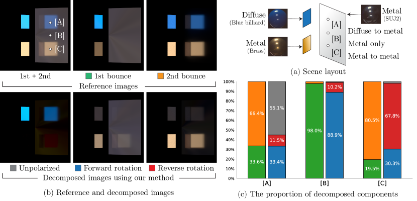
Figure 4: Evaluation result using synthetic data. (a) We designed the scene using multiple planar objects with different materials to produce three types of mixed reflectance components. (b) We can confirm each decomposed image contains the desired reflectance components. Unpolarized: The blue color regions that are unpolarized light through the diffuse surface. Both 1st and 2nd bounce lights are contained. Forward rotation: The 1st bounce reflection from specular surfaces, mostly entire regions of metal surfaces. Reverse rotation: The 2nd bounce reflection from metal-to-metal surfaces. (c) The proportions of 1st/2nd bounces and Unpolarized/Forward/Reverse components on three points [A]-[C]. The points [A] and [C] contain the 2nd reflection from the left side. All points also contain the 1st reflection.

In this section, we evaluate the proposed method using synthetic data. To generate the data, we used Mitsuba 3 [36], which can simulate the light transport of polarization. We used the measured polarized-BRDF data [32] to simulate physically accurate polarization material. We selected Brass and SUJ2 as metal material and Blue billiard as diffuse material based on the visual clarity of the rendered image. The scene layout is shown in Fig. 4(a). We arranged the scene with three planar objects in a V-shape so that inter-reflection occurred. The camera and light source are placed close enough together. This light source illuminates the entire scene.

Fig. 4(b) shows the result of rendered images. The top-left image shows the rendered image consisting of both 1st and 2nd bounce of light. Each component is independently rendered by limiting the maximum number of light bounces in Mitsuba 3 renderer. The bottom row shows the decomposed images by using the proposed method. We can confirm each decomposed image contains desired reflection components as explained in Sec. IV.

Fig. 4(c) shows the proportion of decomposed components at point [A]/[B]/[C]. From this chart, we can observe the following:

• In point [A], the 2nd bounce component is caused by inter-reflection from the blue billiard on the left. As the reflection from the blue billiard is primarily diffuse, this 2nd bounce component is dominated by unpolarized light. The remaining reverse rotation component originates from the specular reflection component of the blue billiard. Additionally, at point [A], there is 1st bounce component observed from the right metal plate of the SUJ2, corresponding to the forward component caused by direct illumination from the light source.

• In point [B], as it is not affected by inter-reflection, almost all the reflected light comes from the 1st bounce, corresponding to the forward rotation component.

• In point [C], same as point [A], we also observe a mixture of 1st and 2nd bounce components. The 2nd bounce component is mainly dominated by the reverse component because it comes from the reflection of Brass material, which has strong specular reflection.

Through this result, we confirm that the decomposed components are matched to the 1st and 2nd components.

VI Experimental Results

Fig. 5 shows the capturing setup for real scenes. The target scene is illuminated by a light source with a linear polarizer attached to the front and measured by a polarization camera (FLIR, BFS-U3-51S5P-C). This polarization camera can capture the polarization state with a single shot. It is equivalent to a conventional camera with a rotating polarizer. Our method specifically targets specular reflection, which is typically required to capture a high dynamic range (HDR) image. Therefore, we captured sequence images with different exposure times and merged them into a HDR image. We acquire multiple HDR images for every polarizer angle of the light side. As explained in Sec IV-D, theoretically, the minimum number of images is two, but we captured four images with different polarizer angles on the light source ($\theta_{l}={0,45,90,135}$) in this experiment to be robust to the sensor noise. The measurements were conducted in a darkroom to avoid the environment light.

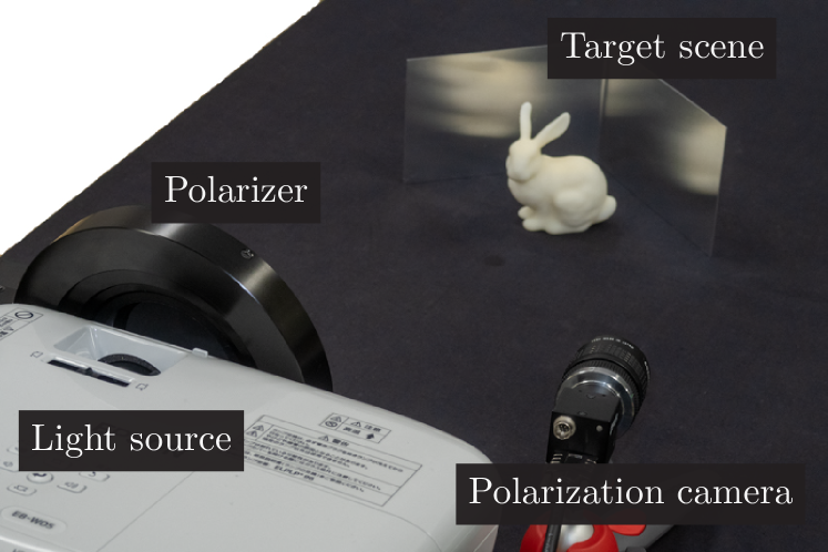
Figure 5: Experimental setup for the real scene. The target scene is illuminated by a light source with a linear polarizer attached to the front and measured by a polarization camera.

VI-A Decomposition of Reflection Components

Fig. 6 shows the decomposed result in the real scenes. Our method successfully decomposes the desired reflectance components for various scenes. The reverse components have a majority of specular inter-reflection for various geometry and metallic materials.

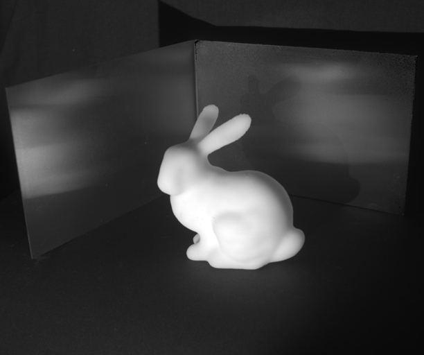
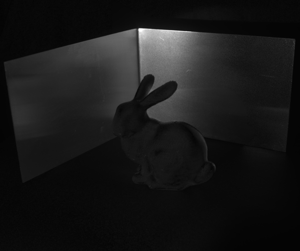
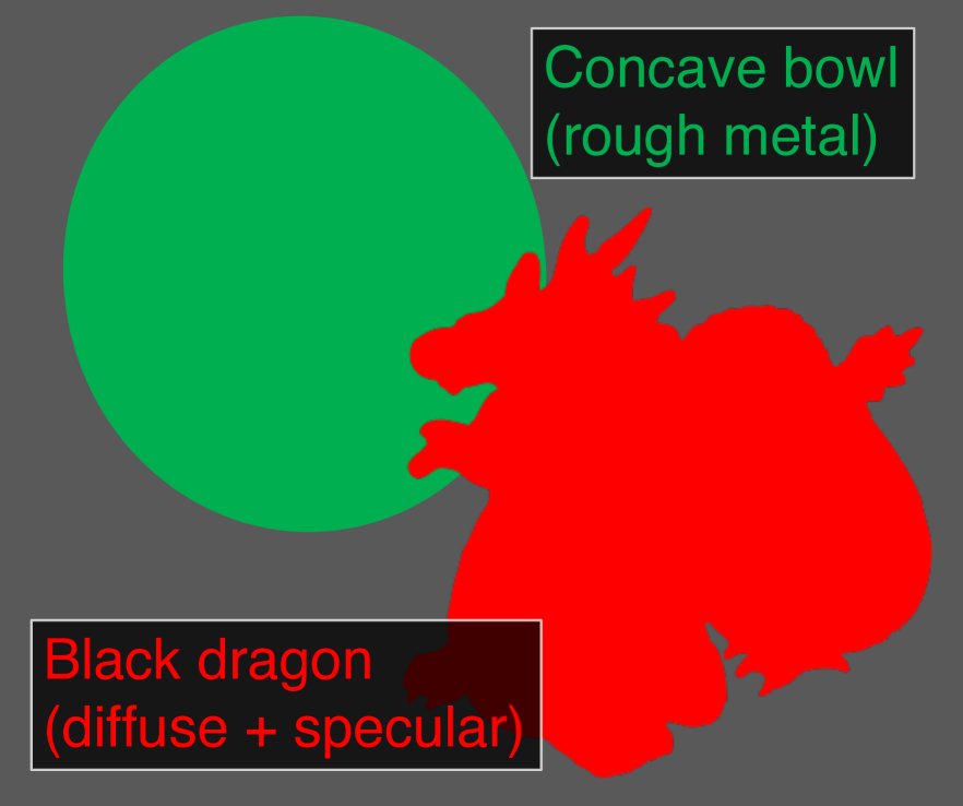
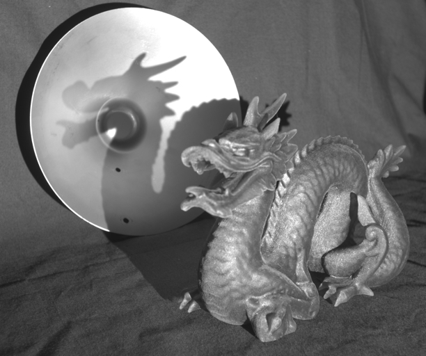
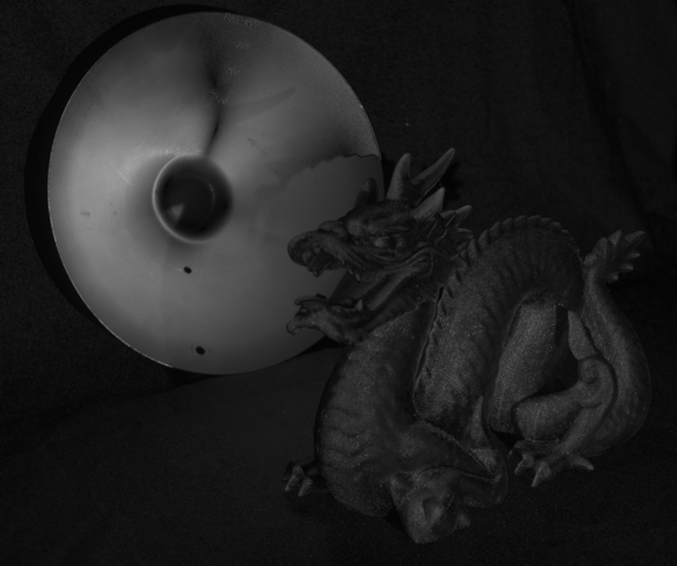
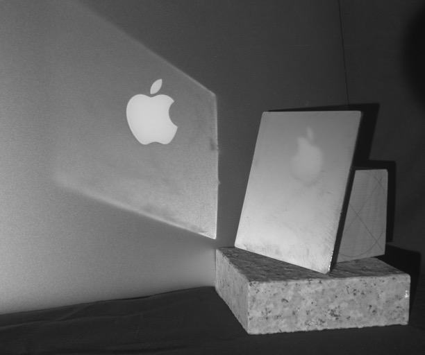
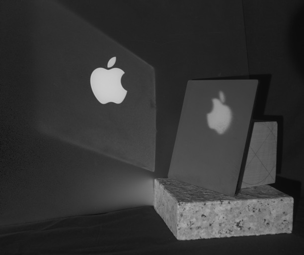
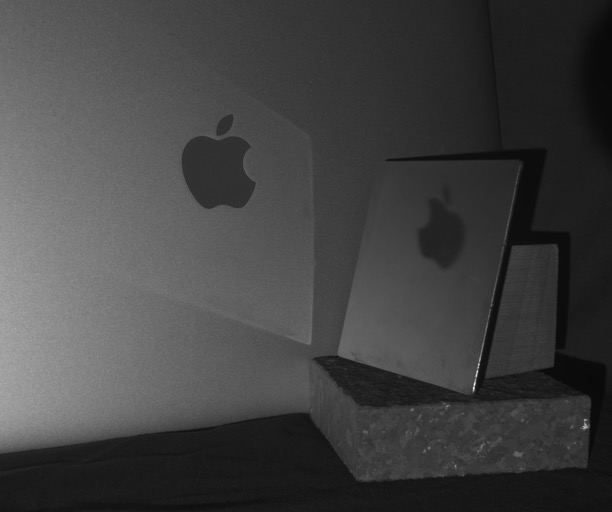
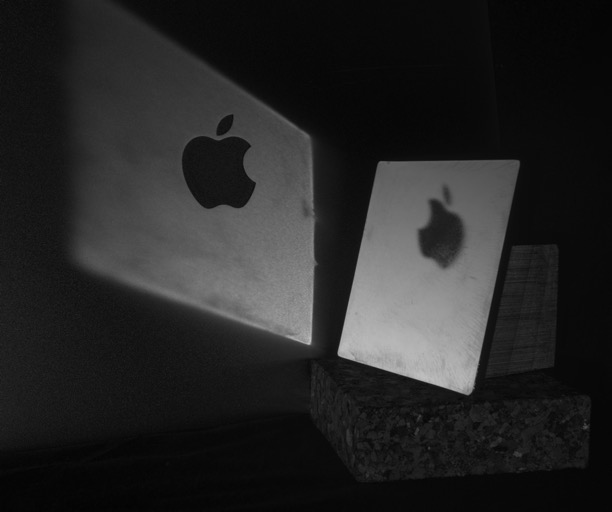
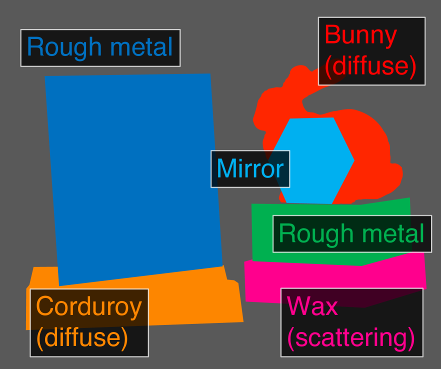
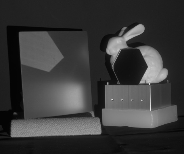
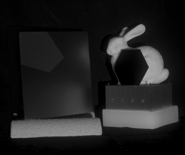
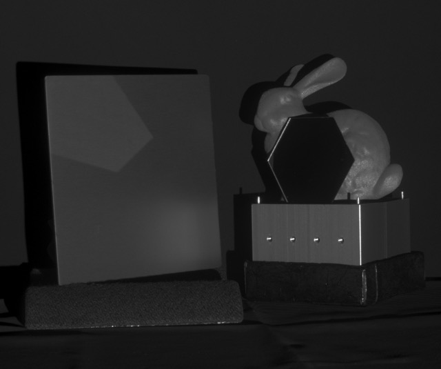
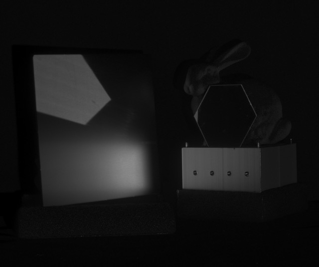
Figure 6: Decomposition results for various scenes. Each column shows the images of the scene layout, regular (sum of all components), unpolarized, forward rotation, and reverse rotation components. Our method can extract specular inter-reflection of metal objects, as shown in the reverse rotation component for various scenes.

VI-B Comparison with high-frequency illumination method

Compared to the other decomposition methods, our method can analyze specular inter-reflection regardless of the spatial frequency response. We compare our method with Nayar’s high-frequency illumination method. Their method can decompose direct and global (including inter-reflection) light components. However, as their paper mentioned, their method fails to decompose high-frequency specular inter-reflection. Fig. 7 shows the comparison of decomposition results. We can confirm that Nayar’s method fails to decompose high-frequency specular inter-reflection from the hexagon-shaped mirror. In contrast, our method successfully extracts specular inter-reflection.

Regular (all)

Direct

Global

Reverse rotation $I_{R}$

Figure 7: Comparison with Nayar’s high-frequency illumination method for specular inter-reflection. This scene contains two types of specular inter-reflection categorized as global components but have distinct spatial frequency responses. Nayar’s method failed to separate high-frequency inter-reflection from the hexagonal mirror. In contrast, our method extracts both specular inter-reflection regardless of its frequency response.

VI-C Combination with high-frequency illumination method

Our decomposition method utilizes polarization as a cue, which does not cause any conflicts with other cues like spatial-frequency and time-of-flight based methods. Fig. 8 shows the results of the combination of Nayar’s method. By combining the different methods, we can achieve a detailed analysis of light transport.

Regular (all)

Scene layout

Figure 8: Combining with Nayar’s decomposition method. This combination allows us to decompose mixed light into six components. Row: Direct / Global components with Nayar’s method [7]. Column: Unpolarized / Forward / Reverse components (ours).

VI-D 3D Measurement for Specular Inter-reflection

As an application, we utilize our decomposition method for 3D measurement with the projector-camera system. Active lighting methods (e.g., structured-light, photometric stereo, and time-of-flight), including the projector-camera system, sometimes struggle with the inter-reflection. This is because these methods assume only direct reflection, which can be problematic when measuring metallic objects with strong specular inter-reflection. Our decomposition method reduces the specular inter-reflection and enables robust measurement of metal objects.

Fig. 9 shows the results of 3D measurement with and without our method. In this experiment, we use the Gray code pattern as structured light. To reduce the specular inter-reflection, we used the forward rotation intensity to estimate 3D points. In the traditional method without decomposition, inter-reflection causes errors in most areas. On the other hand, using the forward rotation component expands the region of the correct points.

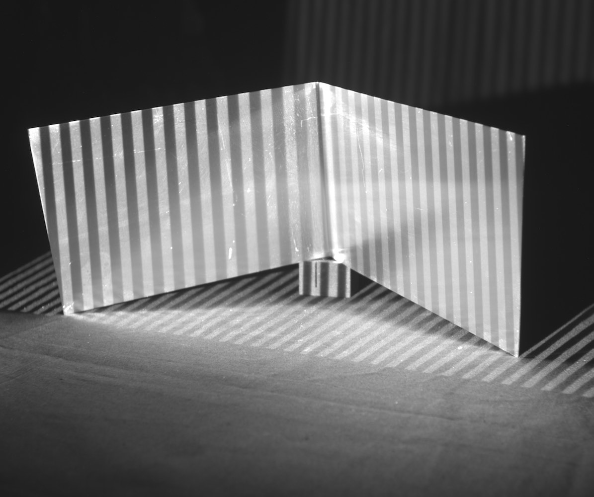
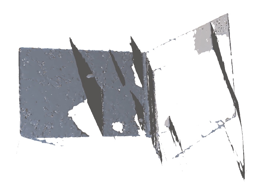
(a) Regular

(completeness=54.6%)

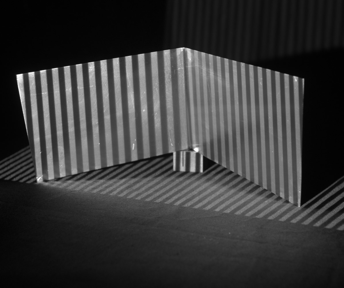
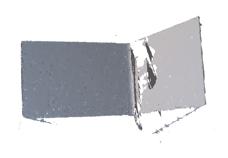
(b) Forward rotation

(completeness=92.8%)

Figure 9: Application for 3D measurement under strong specular inter-reflection. We measure the V-groove metal object using Gray code structured light. Top row: Captured scenes that projected a Gray code pattern. Bottom row: 3D reconstruction results. (a) The regular components cause gross errors. The correct area is only 54.6%. (b) With our method, by using the forward rotation components, the correctly measured area increases to 92.8%.

VII Discussion

VII-A Why Not Circular Polarization?

We proposed a measurement method by rotating the plane of linearly polarized light in order to decompose the reflected components. We clarify why we use linear polarization instead of using circular polarization. Similar to the case of linear polarization discussed in Sec.III, the left- or right-hand circular polarization flips between single and double bounce reflection [33]. We can utilize circular polarization to distinguish direct and inter-reflection, as long as they are not mixed. However, it becomes impossible to decompose if both reflection components are mixed because the incoherent mixture of right-hand and left-hand circular polarized light is observed as unpolarized. That is why we can not use circular polarization alone for this purpose.

VII-B Phase of AoLP

Since the experimental results only showed the intensity images, here we show and describe the phase ($\phi_{F}$ and $\phi_{R}$) obtained from our decomposition method. Fig. 10 shows the phase image of forward and reverse rotation components. The phase of the forward component is near zero for all pixels because direct reflection does not change the polarization phase. We can also see this fact from the plot of direct reflection shown in Fig. 3(b), where the intercept is zero. In contrast, the phase of the reverse component varies depending on the direction from where the first bounce light is coming. For instance, the horizontal and vertical directions do not cause a phase shift, while the oblique directions result in a phase shift. This fact can also be seen from the [C] in Fig.3(b). Currently, we do not use this phase information, but it can potentially analyze the scene geometry.

Intensity

Phase (forward) $\phi_{F}$

Phase (reverse) $\phi_{R}$

Intensity

Figure 10: Visualization of phase components. The scene setup is identical to Fig. 3. The phase values are colored by mapping them to the Hue circle, and the Brightness is modulated by the decomposed intensities.

VIII Conclusion

In this study, we proposed a novel decomposition method of reflection components by featuring the rotation direction of the polarization plane. Our proposed method enables us to decompose the specular inter-reflections, which had been difficult to handle in the past. We verified the effectiveness of our method in both synthetic and real data. Our method can be combined with other methods to explore a detailed analysis of light transport. As an application of 3D measurement, our method reduced the error that occurred by strong specular inter-reflection.

[Solving the Decomposition Equation]

This appendix describes the transformation to solve Eq. 6. At the beginning, we convert Eq. 2 into linear form,

$$I(\theta_{c},\theta_{l})=\mathbf{w}(\theta_{c},\theta_{l})\mathbf{X},$$ (7)

where matrices of known values $W$ and unknown parameters $\mathbf{X}$ are described as follows.

$$\mathbf{w}(\theta_{c},\theta_{l})=\begin{bmatrix}1\\ \cos{2\theta_{c}}\cos{2\theta_{l}}\\ \sin{2\theta_{c}}\sin{2\theta_{l}}\\ \cos{2\theta_{c}}\sin{2\theta_{l}}\\ \sin{2\theta_{c}}\cos{2\theta_{l}}\end{bmatrix},$$ (8)

$$\mathbf{X}=\begin{bmatrix}x_{1}\\ x_{2}\\ x_{3}\\ x_{4}\\ x_{5}\end{bmatrix}=\frac{1}{2}\begin{bmatrix}I_{U}+I_{F}+I_{R}\\ I_{F}\cos{2\phi_{F}}+I_{R}\cos{2\phi_{R}}\\ -I_{F}\cos{2\phi_{F}}+I_{R}\cos{2\phi_{R}}\\ I_{F}\sin{2\phi_{F}}-I_{R}\sin{2\phi_{R}}\\ I_{F}\sin{2\phi_{F}}+I_{R}\sin{2\phi_{R}}\end{bmatrix}.$$ (9)

Suppose we capture $N$ frames while rotating the polarizers of camera ($\theta_{c}=\theta_{c_{1}},\theta_{c_{2}},\cdots,\theta_{c_{N}}$) and light source ($\theta_{l}=\theta_{l_{1}},\theta_{l_{2}},\cdots,\theta_{l_{N}}$), and get a sequence of intensities $I(\theta_{c_{k}},\theta_{l_{k}})$ and vectors $\mathbf{w}(\theta_{c_{k}},\theta_{l_{k}})$. We can stack them as the column vector $\mathbf{I}$ and the matrix $\mathbf{W}$ as follows

$$\mathbf{I}=\begin{bmatrix}I(\theta_{c_{1}},\theta_{l_{1}})\\ I(\theta_{c_{2}},\theta_{l_{2}})\\ \vdots\\ I(\theta_{c_{N}},\theta_{l_{N}})\end{bmatrix},\mathbf{W}=\begin{bmatrix}-&\mathbf{w}(\theta_{c_{1}},\theta_{l_{1}})&-\\ -&\mathbf{w}(\theta_{c_{2}},\theta_{l_{2}})&-\\ &\vdots&\\ -&\mathbf{w}(\theta_{c_{N}},\theta_{l_{N}})&-\end{bmatrix}.$$ (10)

and we can extend Eq. 7 to

$$\mathbf{I}=\mathbf{W}\mathbf{X}.$$ (11)

To solve the above equation, the matrix $\mathbf{W}$ must have its own inverse matrix. Fortunately, if we choose the combination of $(\theta_{c},\theta_{l})$ carefully, $\mathbf{W}$ becomes invertible (we discuss it later). If we have more than five observations ($N\geq 5$), we can use the pseudo-inverse matrix of $\mathbf{W}$ to be robust to the sensor noise. With the pseudo-inverse matrix $\mathbf{W}^{+}$, we can solve $\mathbf{X}$ as follows

$$\begin{split}\mathbf{X}&=(\mathbf{W}^{T}\mathbf{W})^{-1}\mathbf{W}^{T}\mathbf{I}\\ &=\mathbf{W}^{+}\mathbf{I}.\end{split}$$ (12)

By using solved $\mathbf{X}$, we can calculate the parameters of each reflection component $I_{U},I_{F},\phi_{F},I_{R},\phi_{R}$. The relationships among $x_{2},x_{3},x_{4},x_{5}$ is

$$x_{2}-x_{3} =I_{F}\cos{2\phi_{F}}$$ (13)

$$x_{4}+x_{5} =I_{F}\sin{2\phi_{F}}$$ (14)

$$x_{2}+x_{3} =I_{R}\cos{2\phi_{R}}$$ (15)

$$-x_{4}+x_{5} =I_{R}\sin{2\phi_{R}}$$ (16)

then we can calculate the parameters as follows.

Forward rotation component:

$$I_{F} =\sqrt{(x_{2}-x_{3})^{2}+(x_{4}+x_{5})^{2}}$$ (17)

$$\phi_{F} =\frac{1}{2}\arctan{\frac{x_{4}+x_{5}}{x_{2}-x_{3}}}$$ (18)

Reverse rotation component:

$$I_{R} =\sqrt{(x_{2}+x_{3})^{2}+(-x_{4}+x_{5})^{2}}$$ (19)

$$\phi_{R} =\frac{1}{2}\arctan{\frac{-x_{4}+x_{5}}{x_{2}+x_{3}}}$$ (20)

Unpolarized component:

$$I_{U}=2x_{1}-I_{F}-I_{R}$$ (21)

The computational cost of the above algorithm is minimal because we can precompute the pseudo-inverse matrix $\mathbf{W}^{+}$ and easily parallelize per pixel.

To solve Eq. 11, the matrix $\mathbf{W}$ must have its own inverse matrix. Fortunately, if we choose the combinations of $(\theta_{c},\theta_{l})$ carefully, $\mathbf{W}$ becomes invertible. For example, $\mathbf{W}$ for a combination of $\{(\theta_{c},\theta_{l})\}=\{(0,0),(45,45),(0,45),(45,0),(90,0)\}$ is

$$\mathbf{W}=\begin{bmatrix}1&1&1&1&1\\ 1&0&0&0&-1\\ 0&1&0&0&0\\ 0&0&1&0&0\\ 0&0&0&1&0\\ \end{bmatrix},$$ (22)

and this $\mathbf{W}$ is full-rank, so pseudo-inverse matrix $\mathbf{W}^{+}$ is calculable.

References

- [1] S. A. Shafer, “Using color to separate reflection components,” Color Research & Application, vol. 10, no. 4, pp. 210–218, 1985.
- [2] G. J. Klinker, S. A. Shafer, and T. Kanade, “The measurement of highlights in color images,” International Journal of Computer Vision, vol. 2, no. 1, pp. 7–32, 1988.
- [3] Y. Sato and K. Ikeuchi, “Temporal-color space analysis of reflection,” JOSA A, vol. 11, no. 11, pp. 2990–3002, 1994.
- [4] Y. Sato, M. D. Wheeler, and K. Ikeuchi, “Object shape and reflectance modeling from observation,” in Proceedings of the 24th annual conference on Computer graphics and interactive techniques, 1997, pp. 379–387.
- [5] R. T. Tan and K. Ikeuchi, “Separating reflection components of textured surfaces using a single image,” in Digitally Archiving Cultural Objects. Springer, 2008, pp. 353–384.
- [6] H. Kim, H. Jin, S. Hadap, and I. Kweon, “Specular reflection separation using dark channel prior,” in Proceedings of the IEEE conference on computer vision and pattern recognition, 2013, pp. 1460–1467.
- [7] S. K. Nayar, G. Krishnan, M. D. Grossberg, and R. Raskar, “Fast separation of direct and global components of a scene using high frequency illumination,” in ACM SIGGRAPH 2006 Papers, 2006, pp. 935–944.
- [8] M. O’Toole, R. Raskar, and K. N. Kutulakos, “Primal-dual coding to probe light transport.” ACM Trans. Graph., vol. 31, no. 4, pp. 39–1, 2012.
- [9] M. O’Toole, J. Mather, and K. N. Kutulakos, “3d shape and indirect appearance by structured light transport,” in Proceedings of the IEEE Conference on Computer Vision and Pattern Recognition, 2014, pp. 3246–3253.
- [10] M. O’Toole, S. Achar, S. G. Narasimhan, and K. N. Kutulakos, “Homogeneous codes for energy-efficient illumination and imaging,” ACM Transactions on Graphics (ToG), vol. 34, no. 4, pp. 1–13, 2015.
- [11] K. Tanaka, N. Ikeya, T. Takatani, H. Kubo, T. Funatomi, V. Ravi, A. Kadambi, and Y. Mukaigawa, “Time-resolved far infrared light transport decomposition for thermal photometric stereo,” IEEE Transactions on Pattern Analysis and Machine Intelligence, vol. 43, no. 6, pp. 2075–2085, 2019.
- [12] L. B. Wolff and T. E. Boult, “Constraining object features using a polarization reflectance model,” Phys. Based Vis. Princ. Pract. Radiom, vol. 1, p. 167, 1993.
- [13] V. Müller, “Elimination of specular surface-reflectance using polarized and unpolarized light,” in European Conference on Computer Vision. Springer, 1996, pp. 625–635.
- [14] P. Debevec, T. Hawkins, C. Tchou, H.-P. Duiker, W. Sarokin, and M. Sagar, “Acquiring the reflectance field of a human face,” in Proceedings of the 27th annual conference on Computer graphics and interactive techniques, 2000, pp. 145–156.
- [15] Y. Y. Schechner, S. G. Narasimhan, and S. K. Nayar, “Instant dehazing of images using polarization,” in Proceedings of the 2001 IEEE Computer Society Conference on Computer Vision and Pattern Recognition. CVPR 2001, vol. 1. IEEE, 2001, pp. I–I.
- [16] Y. Y. Schechner and N. Karpel, “Recovery of underwater visibility and structure by polarization analysis,” IEEE Journal of oceanic engineering, vol. 30, no. 3, pp. 570–587, 2005.
- [17] W.-C. Ma, T. Hawkins, P. Peers, C.-F. Chabert, M. Weiss, P. E. Debevec et al., “Rapid acquisition of specular and diffuse normal maps from polarized spherical gradient illumination.” Rendering Techniques, vol. 2007, no. 9, p. 10, 2007.
- [18] A. Ghosh, T. Chen, P. Peers, C. A. Wilson, and P. Debevec, “Circularly polarized spherical illumination reflectometry,” in ACM SIGGRAPH Asia 2010 papers, 2010, pp. 1–12.
- [19] V. Couture, N. Martin, and S. Roy, “Unstructured light scanning to overcome interreflections,” in 2011 International Conference on Computer Vision. IEEE, 2011, pp. 1895–1902.
- [20] M. Gupta and S. K. Nayar, “Micro phase shifting,” in 2012 IEEE Conference on Computer Vision and Pattern Recognition. IEEE, 2012, pp. 813–820.
- [21] M. Gupta, A. Agrawal, A. Veeraraghavan, and S. G. Narasimhan, “A practical approach to 3d scanning in the presence of interreflections, subsurface scattering and defocus,” International journal of computer vision, vol. 102, no. 1, pp. 33–55, 2013.
- [22] D. Wu, A. Velten, M. O’Toole, B. Masia, A. Agrawal, Q. Dai, and R. Raskar, “Decomposing global light transport using time of flight imaging,” International journal of computer vision, vol. 107, no. 2, pp. 123–138, 2014.
- [23] T. Chen, H. P. Lensch, C. Fuchs, and H.-P. Seidel, “Polarization and phase-shifting for 3d scanning of translucent objects,” in 2007 IEEE conference on computer vision and pattern recognition. IEEE, 2007, pp. 1–8.
- [24] A. M. Wallace, B. Liang, E. Trucco, and J. Clark, “Improving depth image acquisition using polarized light,” International Journal of Computer Vision, vol. 32, no. 2, pp. 87–109, 1999.
- [25] D. Miyazaki, R. T. Tan, K. Hara, and K. Ikeuchi, “Polarization-based inverse rendering from a single view,” in Computer Vision, IEEE International Conference on, vol. 3. IEEE Computer Society, 2003, pp. 982–982.
- [26] A. Kadambi, V. Taamazyan, B. Shi, and R. Raskar, “Polarized 3d: High-quality depth sensing with polarization cues,” in Proceedings of the IEEE International Conference on Computer Vision, 2015, pp. 3370–3378.
- [27] Y. Ding, Y. Ji, M. Zhou, S. B. Kang, and J. Ye, “Polarimetric helmholtz stereopsis,” in Proceedings of the IEEE/CVF International Conference on Computer Vision, 2021, pp. 5037–5046.
- [28] D. Miyazaki, M. Kagesawa, and K. Ikeuchi, “Transparent surface modeling from a pair of polarization images,” IEEE Transactions on Pattern Analysis and Machine Intelligence, vol. 26, no. 1, pp. 73–82, 2004.
- [29] T. Treibitz and Y. Y. Schechner, “Active polarization descattering,” IEEE transactions on pattern analysis and machine intelligence, vol. 31, no. 3, pp. 385–399, 2008.
- [30] A. Kalra, V. Taamazyan, S. K. Rao, K. Venkataraman, R. Raskar, and A. Kadambi, “Deep polarization cues for transparent object segmentation,” in Proceedings of the IEEE/CVF Conference on Computer Vision and Pattern Recognition, 2020, pp. 8602–8611.
- [31] S.-H. Baek, D. S. Jeon, X. Tong, and M. H. Kim, “Simultaneous acquisition of polarimetric svbrdf and normals,” ACM Trans. Graph., vol. 37, no. 6, pp. 268–1, 2018.
- [32] S.-H. Baek, T. Zeltner, H. Ku, and I. Hwang, “Image-based acquisition and modeling of polarimetric reflectance,” ACM Trans. Graph., vol. 39, no. 4, 2020.
- [33] S.-H. Baek and F. Heide, “Polarimetric spatio-temporal light transport probing,” ACM Transactions on Graphics (TOG), vol. 40, no. 6, pp. 1–18, 2021.
- [34] ——, “All-photon polarimetric time-of-flight imaging,” in Proceedings of the IEEE/CVF Conference on Computer Vision and Pattern Recognition, 2022, pp. 17 876–17 885.
- [35] E. Collett, “Field guide to polarization.” Spie Bellingham, WA, 2005.
- [36] W. Jakob, S. Speierer, N. Roussel, M. Nimier-David, D. Vicini, T. Zeltner, B. Nicolet, M. Crespo, V. Leroy, and Z. Zhang, “Mitsuba 3 renderer,” 2022, https://mitsuba-renderer.org.