Reconstruction of dynamical systems from data without time labels

Abstract

In this paper, we study the method to reconstruct dynamical systems from data without time labels. Data without time labels appear in many applications, such as molecular dynamics, single-cell RNA sequencing etc. Reconstruction of dynamical system from time sequence data has been studied extensively. However, these methods do not apply if time labels are unknown. Without time labels, sequence data becomes distribution data. Based on this observation, we propose to treat the data as samples from a probability distribution and try to reconstruct the underlying dynamical system by minimizing the distribution loss, sliced Wasserstein distance more specifically. Extensive experiment results demonstrate the effectiveness of the proposed method.

65L09, 34A55, 93B30

1 Introduction

Dynamical models are crucial for enhancing our comprehension of the natural world. Extensive data have been amassed to unveil physical laws across various domains. It is a common situation that the collected scientific data contains features of a large number of samples, typically referred to as point cloud data. In this context, it is reasonable to assume that high-dimensional observations are generated by hidden dynamical systems operating within a low-dimensional space, a concept related to the manifold hypothesis.[13]. On the other hand, a set of observational data may exhibit heterogeneity, determined by underlying latent evolutionary laws. Reconstructing an evolutionary trajectory, and even more challengingly, unveiling hidden dynamics from point cloud data lacking time labels, furnishes vital insights for deducing underlying mechanisms across various scientific disciplines.

System Identification

Traditional system identification problem in time series observes trajectory data with time labels $\{(t_{i},\boldsymbol{x}_{i})\}_{i=1}^{n}$ and seek for the representation dynamic $\boldsymbol{x}_{\boldsymbol{\theta}}(t)$ or the differential form $\frac{d\boldsymbol{x}}{dt}=\boldsymbol{f}(\boldsymbol{x},\boldsymbol{\theta})$ that approximates the trajectory. Accurate determination of parameters is crucial for elucidating the underlying dynamics of observed systems. A comprehensible and analytical representation is of particular significance in first-principles-based and phenomenological models. The prevailing direct estimation approach, which relies on a forward-solver, can be distilled into four steps: (1) proposing an initial set of parameters, (2) solving the forward process for the collocation points utilizing a numerical solver, (3) comparing the generated solution with observational samples and updating the parameters accordingly, and (4) iterating steps (2) and (3) until the convergence criteria are satisfied. As a well-established topic, [1] and [21] provide a comprehensive overview of extant results. A direct comparison of evolving trajectory of differential equations forces the simulation error descent within a supervised framework, but is challenged by many numerical issue. The optimization is intrinsically non-convex, culminating in the sensitivity to the initial guess of parameters; concurrently, in order to achieve a stable estimation, the utilization of a high-order solver necessitates considerable computational cost.

Recently, the Neural Ordinary Differential Equation (ODE) approach and its derivatives [6] have supplanted the conventional library representation of force terms by employing neural networks, thereby enhancing the model’s representation capacity and substantially alleviating the aforementioned issues.While this method has demonstrated its efficacy in inferring the dynamics in physical systems[37][8][24][16], it still suffers high computational cost and several subsequent investigations have endeavored to mitigate this limitation[11]. Also focusing on generalization, PDE-Net and its improved version design innovative Neural Networks representation for the unknown response within the PDE model, concurrently predicting the dynamics and revealing the concealed PDE models within a forward solver-based supervised learning paradigm. Contrasting with the forward solver-based methodology, an alternative approach ,known as the sparse identification of nonlinear dynamics (SINDy)[5][3], circumvents forward computation by constructing a dictionary of elementary operators likely to emerge in equations, and minimizing the residual of equations with numerical differentiations employing sparse regression. Numerous subsequent studies have augmented the performance of this foundational concept by refining the estimation of differentiation and least square.

Infinite Time Horizon

A scientific example for observation without time labels is Molecular Dynamics. Routine experiment observations are collections of trajectory of millions of particle’s position, thereby constituting an extensive point cloud. Observation state emanating from thermal equilibrium may be regarded as randomly sampled from an infinitely protracted temporal trajectory, in accordance with the canonical distribution theory and the principle of ergodicity. Reconstructing of concealed dynamic attributes of molecules facilitates the discernment of the underlying mechanisms governing numerous materials and biomolecular structures. Such problem can be generalized to the system identification without time label in Infinite Time Horizon. One common modelling approach is to consider the observation data $\{\boldsymbol{x}_{i}\}_{i=1}^{n}$ as samples of the stationary distribution $\rho(\boldsymbol{x})$ of a dynamical system [4][20]by leveraging the results in statistical physics and physical measure [35]. In this setting, the observation $\{\boldsymbol{x}_{i}\}_{i=1}^{n}$ becomes an ensemble and the target is to discover the hidden energy $E(\mathbf{x})$or velocity field $v(\mathbf{x})$. We argue that in the setting of these works the observation are no longer satisfying the 1D manifold assumption and the observation time instants are fixed to uniformly distributed in the time axis.

Finite Time Horizon

In contrast to observations in Molecular Dynamics, Single-cell RNA sequencing (scRNA-seq) is more closely aligned with the Finite Time Horizon setting. Within the realm of Genomics, scRNA-seq datasets provide transcriptomic profiles for thousands of individual cells in the form of high-dimensional point clouds, wherein each element represents the gene expression for a specific cell. Given the presence of the cell life cycle,these datasets can be regarded as random samples drawn from a finite length time trajectory $[0,T]$. Assuming that the data lies on a connected manifold, the core problem in Trajectory Inference in scRNA-seq entails inferring pseudotemporal orderings or assigning cells with a continuous variable (time) as labels. [26] Over the past decade, numerous TI methodologies have been developed to address this intricate inference problem. Early research efforts leveraged manifold learning approaches and clustering techniques to derive pseudo-temporal orderings of data points while adhering to pre-defined topological constraints for the trajectory (linear, cycle, bifurcation, multifurcation, tree, etc.). Contemporary approaches utilize graph-based method [15][33] and deep learning method [10] to obviate the necessity for a priori knowledge of the network topology and enhance robustness. In the setting of TI, the observations are assumed to be sampled i.i.d from the distribution of the cell expression,which can be construed as a uniform distribution of observation time instants. However, to extract the hidden dynamics, a different observation distribution condition leads to profoundly divergent dynamics.

In generalized Finite Time Horizon setting, we assume that the observation time instant $t$ is a known random variable with density $p(t)$ supported on $[t_{0},t_{0}+T]$. Thus the observation particle $\{\boldsymbol{x}_{i}\}_{i=1}^{n}=\{\boldsymbol{x}(t_{i})\}_{i=1}^{n}$ are samples from random vector $\boldsymbol{x}(t)$. With a known finite duration, the data can satisfy the manifold assumption and the target of system identification is to reconstruct $\boldsymbol{x}(t)$.In our paper, we mainly focus on systems driven by ordinary differential equations

$$\left\{\begin{array}[]{c}\frac{d\boldsymbol{x}}{\operatorname{dt}}=\boldsymbol{f}(\boldsymbol{x},\boldsymbol{\theta}),t\in[t_{0},t_{0}+T]\\ \boldsymbol{x}(t_{0})=\boldsymbol{x}_{0}.\end{array}\right.$$

Rigorous mathematical definition of this problem will be will be presented in the subsequent section2. As a related setting, [17] formulate dynamics with random events into so-called stochastic boundary value problem and concurrently approximate the temporal point process of arrival events and the ODE. Nonetheless, this framework necessitates the order of the observation point, which is presumed absent in our problem.

One of our primary objectives entails reconstructing the missing temporal labels, which can be regarded as learning a one-dimensional parametrization of a manifold. This process is intimately connected to manifold learning techniques. Classical manifold learning methods seek to extract low dimensional representations of high dimensional data that preserving geometric structure. One idea is to require the representation to preserve global structures, such as multi-dimensional scaling and its variants like isometric mapping (ISOMAP) [28], uniform manifold approximation and projection (UMAP) [22] etc.Another line of thought seek to find subspace which preserve local structure, among them the representative works are local linear embedding (LLE) [25], Laplacian eigenmaps (LE) [2], t-distributed stochastic neighbor embedding(t-SNE) [30]etc. In the field of generative model, many forms of models try to learn latent representation and distributions to generate real-world high dimensional data, such as variational auto-encoder[18], GANs[14], normalizing flows [19], diffusion models[27][29]. Generative model is usually considered to be good at modelling high dimensional complex distribution with redundant latent dimension and sometimes failed in parametrizing manifold data, which is often referred to as Mode Collapse.[36]

To resolve this issue, we devise a framework for the automated reconstruction of temporal labels and the inference of the associated hidden dynamics of observation trajectories. Observing that the conventional Neural ODE framework is plagued by non-convexity and numerical issues like computational cost and instability, we directly approximate the solution of the hidden dynamics employing a surrogate model and estimate its form utilizing an alternating direction optimization technique. The temporal labels is obtained by projecting the observation particle onto the acquired solution curve, while the discerned parameter is fine-tuned through a subsequent Neural-ODE-inspired algorithm Main advantages of our work include:

1. Accurate system identification: Obtaining an accurate preliminary approximation, our approach utilizes a forward-based estimator to obtain refined estimation of parameters, crucial for systems exhibiting sensitivity to its parameters. We direct compare the generated solution with the observed trajectory to ascertain the inferred dynamics exhibit sufficient proximity in the forward procession. We demonstrate this capability in intricate dynamic systems such as Lorenz63 and Lotka-Volterra.

2. Efficient reconstruction of the time labels. Instead of learning the parametrization of ODE systems, we directly approximate the solution function to avoid performing forward solves and thus gain high learning efficiency. Using the alternating direction optimization, we not only obtain accurate time label but also receive relatively close guess of parameters in ODE system even for some with complex structure.

3. Applicable to arbitrary distribution: The observation distribution makes great impact on the hidden parameters of trajectory. Our method put the observation distribution into consideration to infer parameters in more general cases compare to other manifold representation learning work. Therefore, we are able to reconstruct velocity and time labels in the right scale.

The organization of the paper is as follows: In Section 2, we present a brief review of works in related domains. Subsequently, in Section 3, we explicate the mathematical formulation of our focal problem. The ensuing Section 4 introduce Sliced Wasserstein Distance, Neural ODE and Trajectory Segmentation, the three fundamental tools employed in our approach. Section 5 explain the process in which our method estimates the parametrization of the hidden dynamics and reconstructs the temporal label, wherein we partition the algorithm into two distinct phases. Main results and some discussions are summarized in Section 6, followed by the conclusion of our research and an exploration of prospective avenues in Section 7.

2 Problem Statement

Model of Measurements

Consider a d-dimensional dynamical system $\boldsymbol{x}(t)=(\boldsymbol{x}_{1}(t),\ldots,\boldsymbol{x}_{d}(t))^{\top}$. The observation instants $t\in\mathbb{R}^{1}$ is a random variable with a known and tractable probability density function $p_{t_{0}}:\mathbb{R}^{1}\rightarrow\mathbb{R}^{1}$ supported on $[t_{0},t_{0}+T]$ (such as uniform distribution $U(t_{0},t_{0}+T)$). The observation samples $\boldsymbol{x}\in\mathbb{R}^{d}$ is thus a random vector which transforms $t$ by the dynamics $\boldsymbol{x}(\cdot)$

(1) $$\boldsymbol{x}=\boldsymbol{x}(t)\quad where\quad t\sim p_{t_{0}}(t).$$

Here we assume the dynamical system $\boldsymbol{x}(t)$ evolves according to the following initial-value problem of autonomous ordinary differential equation

(2) $$\left\{\begin{array}[]{c}\frac{d\boldsymbol{x}}{\operatorname{dt}}=\boldsymbol{f}(\boldsymbol{x},\boldsymbol{\theta}),t\in[t_{0},t_{0}+T]\\ \boldsymbol{x}(t_{0})=(\boldsymbol{x}_{1}(t_{0}),\ldots,\boldsymbol{x}_{d}(t_{0}))^{\top}\in\mathbb{R}^{d},\end{array}\right.$$

where the initial condition $\boldsymbol{x}(t_{0})$ is assumed to be known.

Inference Problem

Suppose the observation data is d-dimensional point cloud generated by random observation of a dynamical system $\boldsymbol{x}(t)$. The observation instants is assumed to be i.i.d and obey the known distribution $t\sim p_{t_{0}}$, and the noisy observation data is thus the random vector $\boldsymbol{x}_{ob}=\boldsymbol{x}(t)+\epsilon$ generated by $t$, where $\epsilon$ is the measurement noise. The general goal is to find a approximating dynamical system $\boldsymbol{x}_{\tilde{\boldsymbol{\theta}}}(t)$

(3) $$\left\{\begin{array}[]{c}\frac{d\boldsymbol{x}_{\boldsymbol{\tilde{\theta}}}}{\operatorname{dt}}=\boldsymbol{f}(\boldsymbol{x},\tilde{\boldsymbol{\theta}}),t\in[t_{0},t_{0}+T]\\ \boldsymbol{x}(t_{0})=(\boldsymbol{x}_{1}(t_{0}),\ldots,\boldsymbol{x}_{d}(t_{0}))^{\top},\end{array}\right.$$

such that the generated random vector $\boldsymbol{x}_{\tilde{\boldsymbol{\theta}}}(t),t\sim p_{t_{0}}$ approach to $\boldsymbol{x}_{ob}$, i.e. $d\left(\boldsymbol{x}_{\tilde{\boldsymbol{\theta}}}(t),\boldsymbol{x}_{ob}\right)$ is small where $d$ is a distributional distance. $\Theta$ is the parametric space which $\tilde{\boldsymbol{\theta}}$ belongs to.

In the real setting, let $\mathbb{X}=\{\boldsymbol{x}_{1},\boldsymbol{x}_{2},\ldots,\boldsymbol{x}_{n}\}$ be discrete-time observed data at $n$ time point $\boldsymbol{t}=(t_{1},\ldots,t_{n})^{\top}$ sampled i.i.d from $p_{t_{0}}$ for the process 2 with known initial condition $\boldsymbol{x}(t_{0})=\boldsymbol{x}_{0}$. We further hope to reconstruct the unknown trajectory ,i.e. the time label $\boldsymbol{t}$ given the observed data $\mathbb{X}$ and the identified dynamical system from (3).

Given that the precise representation of $\boldsymbol{f}(\boldsymbol{x},\boldsymbol{\theta})$ remains inaccessible, the issue becomes intractable. Moreover the periodicity and complexity of the dynamics render simultaneous identification of them ill-posed. Extrinsic noise pervades the particle measurements, contributing to the uncertainty. Future investigations may incorporate intrinsic noise, thereby transforming the dynamics into a stochastic differential equation.

To analyze the uniqueness of the inference problem, we here consider all $C^{1}$ curve in d-dimensional cube $[0,1]^{d}$ as $\mathcal{C}=\{r|r:[0,T]\rightarrow[0,1]^{d}\text{ is }C^{1}\text{ for some }T>0,\|\frac{dr^{\prime}}{dt}\|_{2}>0,\forall t\}$.

We state that the $C^{1}$ trajectory is uniquely determined by the data distribution, the known distribution of observation time instants and initial condition. The proof is provided in AppendixA

Theorem 2.1.

Given the observation distribution $\mathbf{t}\in\mathcal{T}$ with CDF $P(\cdot)\in\mathcal{P}$ ,the observed random vector $\mathbb{X}$ and the initial point $\mathbf{x}_{0}$, the smooth dynamical system $\mathbf{x}(\cdot)\in\mathcal{C}$ that transform $\mathbf{t}$ to $\mathbb{X}$ is unique.

3 Preliminary

3.1 Sliced Wasserstein Distance

For the sake of being self-contained, we give a brief introduction to Sliced Wasserstein Distance(SWD), an important tool we used to measure the difference of data and generated samples. For more complete content, please see [9].

In this section, we consider the Distance between two datasets containing real-world data $x\in\mathcal{D}\subset\mathcal{X}$ and generated data $\tilde{x}=\mathcal{F}_{\theta}(z)\in\mathcal{R}\subset\mathcal{X}$, where $z$ is the sample in latent space and $\mathcal{F}_{\theta}(\cdot)$ is a transformation.

In discrete cases, the quadratic Wasserstein distance $W_{2}^{2}(\mathcal{D},\mathcal{R})$ is defined as

(4) $$W_{2}^{2}(\mathcal{D},\mathcal{R})=\frac{1}{|\mathcal{R}|}\min_{\sigma\in\Sigma_{|\mathcal{R}|}}\sum_{i=1}^{|\mathcal{R}|}\|\mathcal{D}_{\sigma(i)}-\mathcal{R}_{i}\|_{2}^{2}=\frac{1}{|\mathcal{R}|}\min_{P}\sum_{i=1}^{|\mathcal{R}|}\sum_{j=1}^{|\mathcal{D}|}P_{i,j}\|\mathcal{D}_{j}-\mathcal{R}_{i}\|_{2}^{2},$$

where $\mathcal{D}_{i}$ and $\mathcal{R}_{i}$ is the i-th sample in the dataset, $\Sigma_{\mathcal{R}}$ is the set of permutations of $|\mathcal{R}|$ and $P$ is the permutation matrix. Specifically, in one dimentional case where $x\in\mathbb{R}$, such problem has an analytic solution. Let $\sigma_{\mathcal{D}}$ and $\sigma_{\mathcal{R}}$ be the permutations such that

$$\begin{array}[]{c}\mathcal{D}_{\sigma_{\mathcal{D}}(i)}\leq\mathcal{D}_{\sigma_{\mathcal{D}}(i+1)},\hskip 30.00005pt\forall i\\ \mathcal{R}_{\sigma_{\mathcal{R}}(i)}\leq\mathcal{R}_{\sigma_{\mathcal{R}}(i+1)},\hskip 30.00005pt\forall i\end{array}$$

which can be given by sorting both datasets. The optimal permutation for Wasserstein distance defined in 4 is

(5) $$\begin{array}[]{c}\sigma^{\ast}=\sigma_{\mathcal{D}}\sigma_{\mathcal{R}}\\ W_{2}^{2}(\mathcal{D},\mathcal{R})=\frac{1}{|\mathcal{R}|}\sum_{i=1}^{\mathcal{R}}\|\mathcal{D}_{\sigma_{\mathcal{D}}(i)}-\mathcal{R}_{\sigma_{\mathcal{F}}(i)}\|_{2}^{2}\end{array}.$$

We can sort both 1-dimensional data in $\mathcal{O}(|\mathcal{R}|\log|\mathcal{R}|)$. The 1-dimensional case can be extend to high dimentsional using random projections. We can project the data points onto 1-dimensional spaces and integrating the analytical solution of Wasserstein distance over all directions on unit sphere

(6) $$\operatorname{SW}_{2}^{2}(\mathcal{D},\mathcal{R})=\int_{\omega\in\partial B_{1}}W_{2}^{2}(\mathcal{D}^{\omega},\mathcal{R}^{\omega})d\omega,$$

where the sets $\mathcal{D}^{\omega}=\{\omega^{\top}\mathcal{D}_{i}\}_{i=1}^{|\mathcal{D}|},\mathcal{R}^{\omega}=\{\omega^{\top}\mathcal{R}_{i}\}_{i=1}^{|\mathcal{R}|}$ contain the projections of each element onto a specific direction $\omega$.

3.2 Neural ODE

Neural ODE(NODE)[6] is a famous family of deep neural network models that parametrize the neural network as the vector field of an ordinary differential equation. A typical NODE systems can be described as

(7) $$\left\{\begin{array}[]{c}\frac{d\boldsymbol{x}}{\operatorname{dt}}=\boldsymbol{f}(\boldsymbol{x},\tilde{\boldsymbol{\theta}}),t\in[0,t_{N}]\\ \boldsymbol{x}(t_{0})=\boldsymbol{x}_{0}\in\mathbb{R}^{d}.\end{array}\right.$$

where $\boldsymbol{f}(\boldsymbol{x},\tilde{\boldsymbol{\theta}})$ is a neural network. To solve the ODE, one has to employ a numerical scheme ODESolve (e.g. Forward Euler, Runge-Kutta)

$$\tilde{\boldsymbol{x}}(t_{N})=\textit{ODESolve}\left(\boldsymbol{f}(\tilde{\boldsymbol{x}},\tilde{\boldsymbol{\theta}})),\boldsymbol{x}_{0},[0,t_{N}]\right)$$

For a generation problem, the NODE is treated as a probability flow to transform an initial distribution $p_{0}$ in $\mathbb{R}^{d}$ (I.C) to another distribution $p_{T}$ in $\mathbb{R}^{d}$, which translates to an minimization task with the following loss

(8) $$L=\mathbb{E}_{\boldsymbol{x}\sim p_{0},\boldsymbol{y}\sim p_{T}}\left[d\left(\textit{ODESolve}\left(\boldsymbol{f}(\tilde{\boldsymbol{x}},\tilde{\boldsymbol{\theta}}),\boldsymbol{x},[0,t_{N}]\right),\boldsymbol{y}\right)\right].$$

Concerning learning a time-series model , the sequential dataset is given as $\mathcal{D}=\left\{\boldsymbol{x}_{0},\left\{t_{i},\boldsymbol{y}_{i}\right\}_{i=1}^{N}\right\}$,where $\boldsymbol{y}_{i}$ defines the label at time $t_{i}$. To fit the latent dynamic NODE solve the minimization task with the following loss

(9) $$L=\sum_{i=1}^{N}\textit{l}\left(\textit{ODESolve}\left(\boldsymbol{f}(\tilde{\boldsymbol{x}},\tilde{\boldsymbol{\theta}}),\boldsymbol{x}_{0},[0,t_{i}]\right),\boldsymbol{y}_{i}\right).$$

Note that one can generate the trajectory of 9 in a single forward process and update the parameters using Auto-grad. In this case the NODE method can be viewed as a kind of shooting method.

3.3 Trajectory Segmentation

Learning transformation of random variables exhibiting intricate distributions poses a significant challenge. In the context of our problem, a distinct property of the dataset is that it is located on a curve along a curve situated within a high-dimensional space. Leverage the Divide and Conquer strategy, segmenting the long trajectory into short and simple pieces may alleviate the difficulty and numerical issues.

The trajectory segmentation problem can be viewed as a unsupervised clustering challenge. Conventional clustering analysis partitions the datasets into groups, ensuring elevated intra-cluster similarity and diminished inter-cluster similarity. To segment the trajectory, the similarity between particles may be associated with the Euclidean distance or the arc length. Numerous clustering techniques exist for segmenting such manifold-type data into a specified number of classes, such as Agglomerative clustering[23], DBSCAN[12] and Spectral clustering[32].

However, in the task of trajectory segmentation, the challenge lies not only in the grouping of data but also in ascertaining the initial conditions and the observation distribution of each cluster. To this end, we propose an estimation pipeline to serve as a post-processing step for the clustering procedure. Initially, we partition the dataset into non-overlapping continuous trajectory segments $\{\mathbb{X}_{l}\}_{l=1}^{L}$ via unsupervised learning method and we assume that each cluster contains data points from distinct time intervals. To estimate the initial point and observation distribution of each cluster, we consider the trajectory pieces contained the highest number of elements that coincide with $B_{r}(\boldsymbol{x}_{0})$ as the foremost trajectory, where $B_{r}(\boldsymbol{x}_{l})$ denotes the open ball of radius $r$ centered at $\boldsymbol{x}_{l}$. To determine the subsequent trajectory pieces, we adopt the following rules to select tail element from trajectory piece $\mathbb{X}_{l}$ given the initial point $\boldsymbol{x}_{Head,l}$

$$\boldsymbol{x}_{Tail,l}=\mathop{\arg\max}\limits_{\boldsymbol{x}\in\mathbb{X}_{l}\cap B_{R}{\boldsymbol{x}_{Head,l}}}\#\{\boldsymbol{y}|\boldsymbol{y}\in\mathbb{X}_{l}\cap B_{r}(\boldsymbol{x})\},$$

where $\#$ denotes the element number of a set.

We order these trajectory pieces and determine their heads using the above criteria. Finally, we use the two-side truncated distribution to estimate the observation distribution of each trajectory piece. Suppose a trajectory piece contains $n_{l}$ elements and the initial time is $T_{l}$, then the restricted observing instants $\boldsymbol{t}_{l}$ as a random variable is

$$\boldsymbol{t}_{l}=\boldsymbol{t}\mathbb{I}_{T_{l}<\boldsymbol{t}<P_{t_{0}}^{-1}\left(P_{t_{0}}(T_{l})+\frac{n_{l}}{n}\right)}\sim p_{l}$$

where $P_{t_{0}}$ is the probability distribution function of $p_{t_{0}}$ and $\boldsymbol{t}\sim p_{t_{0}}$. That is, wwe employ the frequency to approximate the proportional length of a trajectory segment. Undoubtedly, the segmentation process may encounter failure owing to the overlapping and twining conformation of trajectory, which we defer to further work.Empirically, we discern that Agglomerative clustering exhibits heightened robustness against noise, and as such, our experimentation is based on this clustering technique. We encapsulate the trajectory segmentation methodology in Algorithm 1 and illustrate the segmentation results for several systems in 1.

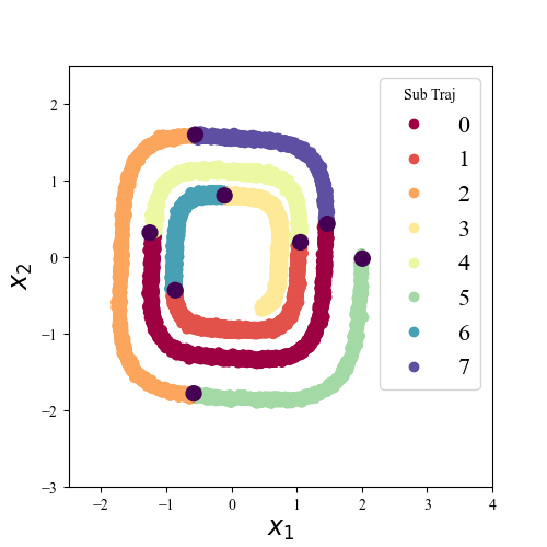
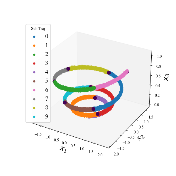
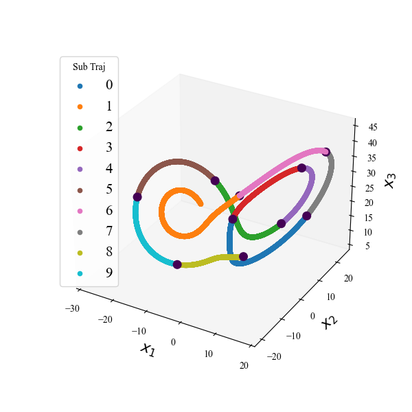
Figure 1: Segmentation result of illustrative problem:(a) is the 8 piece cluster result of Cubic2D ODE system initiate at $(2,0)$ with $T=10$;(b) is the 10 piece cluster result of Linear3D ODE system initiate at $(2,0,-1)$ with $T=10$;(c) is the 10 piece cluster result of Lorenz ODE system initiate at $(10,20,-10)$ with $T=3$.

Algorithm 1 Trajectory segmentation algorithm

  Input: $\mathbb{X},p_{t_{0}},\boldsymbol{x}(t_{0}),T,L$

  $\{\mathbb{X}_{l}\}_{l=1}^{L}=Clustering(\mathbb{X},L)$

  for $l=1:L$ do

     $T_{l}=P_{t_{0}}^{-1}\left(P_{t_{0}}(T_{l-1})+\frac{n_{l}}{n}\right)-T_{l-1}$

     $\boldsymbol{x}(T_{l})=\mathop{\arg\max}\limits_{\boldsymbol{x}\in\mathbb{X}_{l}\cap B_{R}{\boldsymbol{x}(T_{l-1})}}\#\{\boldsymbol{y}|\boldsymbol{y}\in\mathbb{X}_{l}\cap B_{r}(\boldsymbol{x})\},$

      $\boldsymbol{t}_{l}=\boldsymbol{t}\mathbb{I}_{T_{l}<\boldsymbol{t}<P_{t_{0}}^{-1}\left(P_{t_{0}}(T_{l})+\frac{n_{l}}{n}\right)}\sim p_{l}$

  end for

  return  $\{\mathbb{X}_{l}\}_{l=1}^{L},\{T_{l}\}_{0}^{L},\{\boldsymbol{x}(T_{l})\}_{l=0}^{L},\{p_{l}\}_{l=1}^{L}$

4 Methodology

In this section, we present our learning framework to extract an determined dynamical system as the transformation of random variables from data without temporal labels, which utilizes a distributional metrics and physics-informed regularization.

4.1 Overview of Architecture

Inspired by the frameworks presented in [34] and [7], we propose a deep learning-based approach that facilitatesrapid computational acceleration during the initial training phase and offers a more precise preliminary estimation for subsequent parameter inference.

In the Distribution Matching phase, a neural network endeavors to approximate the solution function of Ordinary Differential Equation (ODE) dynamics by iteratively minimizing a distributional distance, while a physics-informed regularization is employed to enforce the requisite smoothness of the solution function and providing a proximate estimate of the hidden dynamics. Given that, during computational experiments, short trajectories are easier to identify than lengthy and intricate ones. Particularly for systems exhibiting complex phase spaces, we initially partition the trajectories into abbreviated segments utilizing an unsupervised clustering technique to render the problem more tractable.

In the Parameter Identification phase, leveraging the learned ODE solution and dictionary representations, we proceed to refine the representation parameter in a Neural-ODE-like way, i.e. by solving a forward parametrized ODE system on time instants sampled from observation distributions and performing gradient descent for distributional metrics iteratively. Comprehensive elaboration on this process will be presented in the subsequent subsections.

4.2 Distribution Matching Phase

In this phase, we want to provide a surrogate model for the ODEs’ solution $\boldsymbol{x}(t)$ from the observation data $\mathbb{X}=\{\boldsymbol{x}_{i}\}_{i=1}^{n}$ with observation instants $\boldsymbol{t}=\{t_{i}\}_{i=1}^{n},t_{i}\sim p_{t_{0}}$ using deep neural networks (DNN). Here DNN can be viewed as a generator, i.e. a multi-dimensional transformation from the prior distribution (observation distribution) to the solution distribution in phase space.

4.2.1 Distribution Matching

We formalize the distribution matching target using Sliced Wasserstein Distance

$$\begin{array}[]{cc}\mathop{\min}\limits_{\tilde{\boldsymbol{\theta}}}&\mathbb{E}_{\mathbb{X}_{\tilde{\boldsymbol{\theta}}}}\operatorname{SW}_{2}^{2}\left(\mathbb{X}{,\mathbb{X}_{\tilde{\boldsymbol{\theta}}}}\right)+\lambda_{\operatorname{init}}\|\boldsymbol{x}_{\tilde{\boldsymbol{\theta}}}(t_{0})-\boldsymbol{x}(t_{0})\|_{2}^{2}+\lambda_{\operatorname{reg}}\operatorname{Reg}(\boldsymbol{x}_{\tilde{\boldsymbol{\theta}}})\\ s.t.&\mathbb{X}_{\tilde{\boldsymbol{\theta}}}=\{\{x_{i}\}_{i=1}^{n}|x_{i}\sim\boldsymbol{x}_{\tilde{\boldsymbol{\theta}}}(t),t\sim p_{t_{0}}\}\end{array},$$

where $\mathbb{X}_{\tilde{\boldsymbol{\theta}}}$ is a $n$-dimensional random variable with the entry as the observation distribution applied by the estimated solution function $\boldsymbol{x}_{\tilde{\boldsymbol{\theta}}}(\cdot)$, $\lambda_{\operatorname{init}}$ is the weight of soft penalty of initial condition and $\operatorname{Reg}(\cdot)$ is the regularization term to avoid overfitting. After segmentation, we obtain trajectory piece $\{\mathbb{X}_{l}\}_{l=1}^{L}$ with estimates of initial condition $\{\boldsymbol{x}_{\operatorname{init},l}\}_{l=1}^{L}$, time length $\left\{T_{l}=\frac{n_{l-1}}{n}\right\}_{l=1}^{L}$ and observation distribution $\{p_{l}\}_{l=1}^{L}$. We propose a piece-wise version of our target function

$$\begin{array}[]{cc}\mathop{\min}\limits_{\tilde{\boldsymbol{\theta}}\in\boldsymbol{\Theta}}&\sum_{l=1}^{L}\mathbb{E}_{\mathbb{X}_{\tilde{\boldsymbol{\theta}},l}}\operatorname{SW}_{2}^{2}\left({\mathbb{X}_{l}}{,\mathbb{X}_{\tilde{\boldsymbol{\theta}},l}}\right)+\sum_{l=1}^{L}\lambda_{\operatorname{init},l}\|\boldsymbol{x}_{\tilde{\boldsymbol{\theta}}}(T_{l})-\boldsymbol{x}(T_{l})\|_{2}^{2}+\lambda_{\operatorname{reg}}\operatorname{Reg}(\boldsymbol{x}_{\tilde{\boldsymbol{\theta}}})\\ s.t.&\mathbb{X}_{\tilde{\boldsymbol{\theta}},l}=\{\{x_{i}\}_{i=1}^{n_{l}}|x_{i}\sim\boldsymbol{x}_{\tilde{\boldsymbol{\theta}}}(\hat{t}),\hat{t}\sim p_{l}(t)\}\end{array}$$

To solve the optimization problem, we employ the following step in each iteration and each trajectory piece:

1. Uniformly sample $\{x_{i}^{l}\}_{i=1}^{B}$ from $\mathbb{X}_{l}$ and sample $\{t_{j}^{l}\}_{j=1}^{B}$ from $p_{l}(t)$.

2. Calculate the solution $\{\boldsymbol{x}_{\tilde{\boldsymbol{\theta}}}(t_{j}^{l})\}_{j=1}^{B}$ of each sample time instant.

3. Approximate the target function by

   $$\begin{array}[]{lll}L_{{}_{l}}&=&\frac{\lambda_{l}}{\Omega}\sum_{k=1}^{\Omega}\operatorname{W}_{2}^{2}(\{w_{k}^{\top}\boldsymbol{x}_{\tilde{\boldsymbol{\theta}}}(t_{j}^{l})\}_{j=1}^{B},\{w_{k}^{\top}x_{i}^{l}\}_{j=1}^{B})\\ &+&\lambda_{\operatorname{init},l}\|\boldsymbol{x}_{\tilde{\boldsymbol{\theta}}}(T_{l})-\boldsymbol{x}(T_{l})\|_{2}^{2}+\lambda_{\operatorname{reg}}\operatorname{Reg}(\boldsymbol{x}_{\tilde{\boldsymbol{\theta}}})\end{array}$$

   where $\operatorname{Reg}(\boldsymbol{X}_{\tilde{\boldsymbol{\theta}}})$ is computed on a time grid of$[\tau_{l},\tau_{l+1}]$ with uniform stepsize.

4. Update the parameter $\tilde{\boldsymbol{\theta}}$.

Numerous options exist for the regularization term. For instance, one may employ the $H_{1}$ semi-norm regularization term, which imposes an additional smoothness constraint and circumvents discontinuities induced by segmentation. Drawing inspiration from [7], we devise the regularization term as the residual of ODE to combine the distribution matching and parameter identification cohesively. A classical way to combine two target together is using an ODE residual as the regularization term ,which we called it as Physics-informed regularization

$$\operatorname{Reg}(\boldsymbol{x}_{\tilde{\boldsymbol{\theta}}})=\|\boldsymbol{\phi}(\boldsymbol{X})\boldsymbol{\Lambda}-\dot{\boldsymbol{X}}\|_{2}^{2},$$

where $\boldsymbol{X}=[\boldsymbol{x}_{\tilde{\boldsymbol{\theta}}}(t_{1}),\ldots,\boldsymbol{x}_{\tilde{\boldsymbol{\theta}}}(t_{m})]^{\top}\in\mathbb{R}^{m\times d}$ is the value of the neural network solution at a discrete set of m timepoints $\{t_{i}\}_{i=1}^{m}$ with uniform stepsize $\Delta t=\frac{T}{m}$ of $[t_{0},t_{0}+T]$, $\dot{\boldsymbol{X}}=\left[\frac{d\boldsymbol{x}_{\tilde{\boldsymbol{\theta}}}(t_{1})}{\operatorname{dt}},\ldots,\frac{d\boldsymbol{x}_{\tilde{\boldsymbol{\theta}}}(t_{m})}{\operatorname{dt}}\right]^{\top}\in\mathbb{R}^{m\times d}$ is the corresponding derivative provided by automatic differentiation, $\boldsymbol{\phi}(\boldsymbol{X})\in\mathbb{R}^{m\times s}$ is the value of candidates in the library given by

$$\boldsymbol{\phi}(\boldsymbol{X})=\left[\begin{array}[]{cccc}\boldsymbol{f}_{1}(\boldsymbol{X}),&\boldsymbol{f}_{2}(\boldsymbol{X}),&\ldots&\boldsymbol{f}_{s}(\boldsymbol{X})\end{array}\right].$$

To ensure training stability of $\tilde{\boldsymbol{\theta}}$, the Alternating Direction Optimization(ADO) is introduced which freezes $\boldsymbol{\Lambda}$ while training $\tilde{\boldsymbol{\theta}}$ and updates $\boldsymbol{\Lambda}$ every a few iterations. Given the estimated solution function $\boldsymbol{x}_{\tilde{\boldsymbol{\theta}}}$ in the training stage, we update $\boldsymbol{\Lambda}$ via sequential threshold ridge regression (STRidge)

$$\min_{\boldsymbol{\Lambda}}\|\boldsymbol{\phi}(\boldsymbol{X})\boldsymbol{\Lambda}-\dot{\boldsymbol{X}}\|_{2}^{2}+\lambda_{\operatorname{sparse}}\|\boldsymbol{\Lambda}\|_{0}.$$

Sparse identification, a fundamental concept in data analysis, finds its theoretical foundation in the venerable principle of Occam’s Razor. This principle posits that, when elucidating the latent dynamics within data, our foremost objective should be the selection of the simplest model. The act of favoring models with the fewest non-zero coefficients holds multifaceted advantages. It elevates the interpretability of the model and mitigate the risk of overfitting the data, thereby endowing the model with an enhanced capacity for generalization. We present in Algorithm 2 the summary of procedure in the Parameter identification phase.

Algorithm 2 Distribution matching phase algorithm

  Input: $\mathbb{X},p_{t_{0}},\boldsymbol{x}(t_{0}),T,Iter,Iter_{phase1},Iter_{update},Batch$

  $\{\mathbb{X}_{l}\}_{l=1}^{L},\{T_{l}\}_{l=1}^{L},\{\boldsymbol{x}(T_{l})\}_{l=0}^{L-1},\{p_{l}\}_{l=1}^{L}=Cluster(\mathbb{X},T,\boldsymbol{x}(t_{0}))$

  for $Iter=1:Iter$ do

     for $l=1:L$ do

        if $Iter\leq$ $Iter_{phase1}$ then

           Sample $\{t_{j}\}_{j=1}^{Batch}\sim p_{l}$,compute $\{\boldsymbol{x}_{\tilde{\boldsymbol{\theta}}}(t_{j})\}_{j=1}^{Batch}$

           Compute original SWD loss and update $\tilde{\boldsymbol{\theta}}$

        else

           if $Iter\%Iter_{update}=0$ then

              Update$\boldsymbol{\Lambda}$ using STRidge at $\{\hat{t_{j}}=\frac{j}{M}T+t_{0}\}_{j=0}^{M}$

           end if

           Sample $\{t_{j}\}_{j=1}^{Batch}\sim p_{l}$,compute $\{\boldsymbol{x}_{\tilde{\boldsymbol{\theta}}}(t_{j})\}_{j=1}^{Batch}$

           Compute Residual-regularized SWD loss and update $\tilde{\boldsymbol{\theta}}$

        end if

     end for

  end for

  return  $\boldsymbol{x}_{\tilde{\boldsymbol{\theta}}},\boldsymbol{\Lambda}$

4.3 Parameter Identification Phase

In the distribution matching phase, we employ Sparse Regression to obtain an estimated weight $\boldsymbol{\Lambda}$ of the expression library , which shall be regarded as the initial approximation in this stage. To attain precise estimation, we adopt a Neural-ODE-inspired learning framework, as delineated in Section A.1 but applied to trajectory segments. Indeed, in each epoch we sample a few trajectory pieces, wherein each possesse an estimated initial point $\boldsymbol{x}(T_{l})$ and observation distribution $p_{l}$. The contributed loss for each piece is

(10) $$L_{l}=SW_{2}^{2}(\{\boldsymbol{x}_{\boldsymbol{\Lambda}}(t_{i}^{l})\}_{i=1}^{B},\{\boldsymbol{x_{i}^{l}}\}_{i=1}^{B}).$$

where $\{t_{i}^{l}\}_{i=1}^{B}$ is sample i.i.d from $p_{l}$ ,$\{\boldsymbol{x_{i}^{l}}\}_{i=1}^{B}$ is sampled uniformly from $\mathbb{X}_{l}$ and $\boldsymbol{x}_{\boldsymbol{\Lambda}}(t_{i}^{l})=\textit{ODESolve}\left(\boldsymbol{\phi}(\boldsymbol{x}_{\boldsymbol{\Lambda}})\boldsymbol{\Lambda},\boldsymbol{x}(T_{l}),[T_{l},T_{l+1}]\right)$. While back-propagation through a ODE trajectory is costly, incurs a significant computational expense, the shooting method facilitates a direct comparison between the simulated distribution and the empirical data distribution. Given that a reasonably accurate initial approximation is provided by the initial phase, our experiments demonstrate that a limited number of epochs are required to achieve high-quality parameter estimation. Additionally, employing an appropriate batch size establishes a balance between computational time and the quality of the results. To preserve the sparsity of the reconstructed system, we eliminate terms with coefficients below a predetermined threshold following a post-warm-up training phase.

To recovery the observation time of each data point, we here solve the identified IVP at a dense grid $\{\hat{t}_{i}\}_{i=1}^{M},M\gg n$

(11) $$\left\{\begin{array}[]{c}\frac{d\boldsymbol{x}}{\operatorname{dt}}=\boldsymbol{\phi}(\boldsymbol{x})\boldsymbol{\Lambda}_{end},t\in[t_{0},t_{0}+T]\\ \boldsymbol{x}(t_{0})=(\boldsymbol{x}_{1}(t_{0}),\ldots,\boldsymbol{x}_{d}(t_{0}))^{\top}.\end{array}\right.$$

The time labels are obtain by solving an optimization problem

(12) $$\min_{\{t_{j}\}_{j=1}^{n}\subset\{\hat{t}_{i}\}_{i=1}^{M}}\sum_{j=1}^{n}\|\boldsymbol{x}_{j}-\boldsymbol{x}_{\boldsymbol{\Lambda}}(t_{j})\|_{2}^{2}.$$

Such problem can be analytically solved by first computing the $L_{2}$ distance matrix of the generated data and the dataset then take $\arg\max$ for each row.

We present in Algorithm 3 the summary of procedure in the Parameter identification phase.

Algorithm 3 Parameter identification phase algorithm

  Input: $\mathbb{X},p_{t_{0}},T,\boldsymbol{x}(t_{0}),Iter,Batch,\boldsymbol{\Lambda}$

  for $Iter=1:Iter$ do

     for $l=1:L$ do

        Sample $\{t_{i}^{l}\}_{i=1}^{B}\sim p_{l}$

        Obtain $\{\boldsymbol{x}_{\boldsymbol{\Lambda}}^{l}(t_{i})\}_{i=1}^{B}$ by solving IVP with initial condition $\boldsymbol{x}(T_{l})$

        Compute SWD loss $L_{l}$ by 10,$L_{total}=L_{total}+L_{l}$

     end for

     Update $\boldsymbol{\Lambda}$ by gradient descent of $L_{total}$

  end for

  return  $\boldsymbol{\Lambda}$

5 Experiments

In this section, we shall employ our methodology to the elementary demonstrative systems delineated in [5], the Lorenz equations and Duffing equations in the chaotic regime, the Lotka-Volterra systems in high dimensional regime, the pendulum equations in non-polynomial regime. In the following, we will evaluate the precision, the robustness and the efficacy for non-uniform observation distribution of our approach and highlight its advantages.

5.1 Numerical setups and performance metrics

In our experiment, all observation datasets are generated utilizing LSODA method in [31] while the inferred trajectories are computed employing the RK4 scheme to achieve an equilibrium between computational expense and precision. For examples with uniform distribution of observation instants, we employ 50,000 temporal instants for dataset generation and a discrete set of 2000 timepoints with uniform stepsize $\{t_{i}^{\star}\}_{i=0}^{2000}$ is used to assess the error of the learned dynamics. Specifically, to evaluate the performance, we record the Mean Absolute Error(MAE) of every record timepoint $\{\boldsymbol{x}_{\tilde{\boldsymbol{\theta}}}(t_{i}^{\star})\}_{i=1}^{2000}$ as a direct evaluation metric for reconstructing dynamics. To compute the MAE for the identified ODE system, we partition the uniform temporal grid into short intervals according to the estimated time length of each cluster and compute the solution of each short trajectories using the estimated initial points. Subsequently,we combine these solution trajectories to acquire $\{\boldsymbol{x}_{\tilde{\boldsymbol{\theta}}}(t_{i}^{\star})\}_{i=1}^{2000}$. The RMAE of solution is computed by

$$RMAE=\frac{\sum_{i=1}^{2000}|\boldsymbol{x}_{\tilde{\boldsymbol{\theta}}}(t_{i}^{\star})-\boldsymbol{x}(t_{i}^{\star})|}{\sum_{i=1}^{2000}|\boldsymbol{x}(t_{i}^{\star})|}$$

For parameter identification, we use the relative mean absolute error(RMAE)

$$\boldsymbol{E}_{para}=\frac{||\hat{\boldsymbol{\Lambda}}-\boldsymbol{\Lambda}^{\star}||_{1}}{||\boldsymbol{\Lambda}^{\star}||_{1}}$$

where $\hat{\boldsymbol{\Lambda}}$ is the estimated parameters of the dynamical system and $\boldsymbol{\Lambda}^{\star}$ is the ground truth. Regarding the reconstruction of time label, we evaluate RMAE of the reconstructed time labels with ground truth

$$\boldsymbol{E}_{time}=\frac{\sum_{i=1}^{n}|\hat{t}_{i}-t_{i}|}{\sum_{i=1}^{n}|t_{i}|}$$

The surrogate model in our experiment is a 5-layer MLP with 500 neurons in each layer and SiLU activation function. And we choose AdamW as the optimizer for both phases. All the experiment were done on the Nvidia RTX3090 graphics processing unit (GPU) and Intel Xeon Gold 6130 processor with 40G RAM.

5.2 Simple illustrative systems

We here apply the reconstruction algorithm to some simple systems with the following form

$$\left\{\begin{array}[]{c}\frac{d\boldsymbol{x}}{\operatorname{dt}}=\boldsymbol{A}\boldsymbol{f}(\boldsymbol{x}),t\in[0,T]\\ \boldsymbol{x}(0)=(\boldsymbol{x}_{1},\ldots,\boldsymbol{x}_{d})^{\top}.\end{array}\right.$$

1. Linear2D equations:The linear matrix is $A=\begin{bmatrix}-0.1&2\\ -2&-0.1\end{bmatrix}$, the transformation is $\boldsymbol{f}=\mathbb{I}_{d}$ ,the initial condition is $\boldsymbol{x}(0)=[2,0]$, the time length is $T=10$.

2. Cubic2D equations:The linear matrix is $A=\begin{bmatrix}-0.1&2\\ -2&-0.1\end{bmatrix}$, the transformation is $\boldsymbol{f}=\begin{bmatrix}x_{1}^{3}\\ x_{2}^{3}\end{bmatrix}$ ,the initial condition is $\boldsymbol{x}(0)=[2,0]$, the time length is $T=10$.

3. Linear3D equations:The linear matrix is $A=\begin{bmatrix}-0.1&2&0\\ -2&-0.1&0\\ 0&0&-0.3\end{bmatrix}$, the transformation is $\boldsymbol{f}=\mathbb{I}_{d}$ ,the initial condition is $\boldsymbol{x}(0)=[2,0,-1]$, the time length is $T=10$.

The details of implementation parameters are delineated in table 5, and a comprehensive summary of our discoveries is provided in Fig2. In these cases, we employ third-order complete polynomials and exponential functions as the basis for the library in both phases. Our method not only reconstructs the solution and temporal labels with exceptional precision but also accurately identifies the underlying system. Subsequent to the initial training devoid of regularization, the approximate solution derived from the neural network captures a proximate estimation of the hidden system’s trajectory. Employing the guidance of the distilled model, ADO training further refines the solution quality by harnessing a regularity ansatz from ODEs. The MAE curve and parameters’ error curve indicate that while the surrogate model adeptly approximates the solution, the inferred systems still deviate from the observed systems. This deviation is subsequently rectified by the Parameter Identification Phase. The results imply that the identified ODE system provides comparable accuracy for temporal label reconstruction to solutions represented by neural networks. It is vital to recognize that the magnitude of the Physics-informed regularization term may exhibit variability, owing to the inherent properties of the equations themselves, necessitating a balanced approach during the training process.

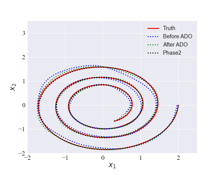
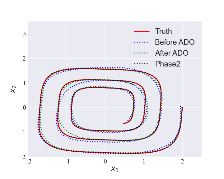
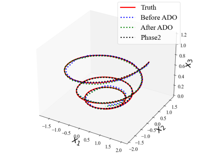
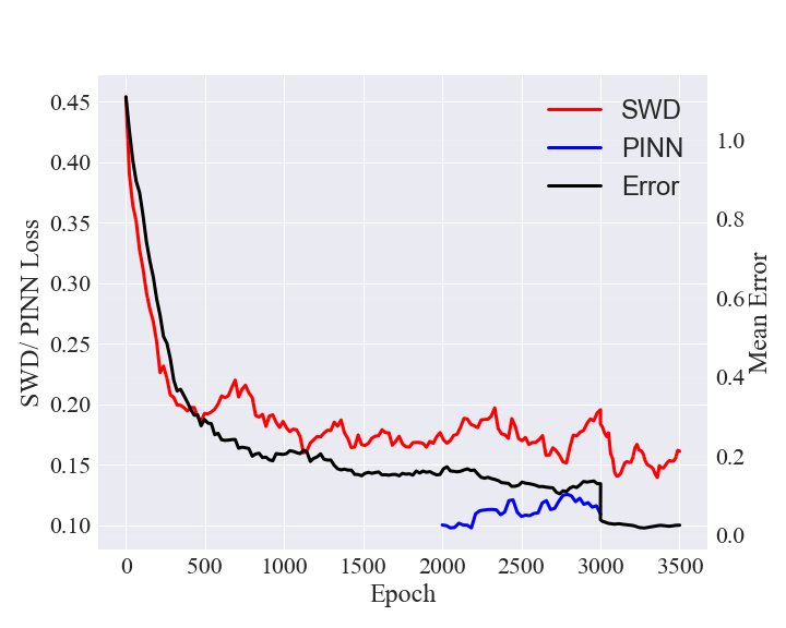
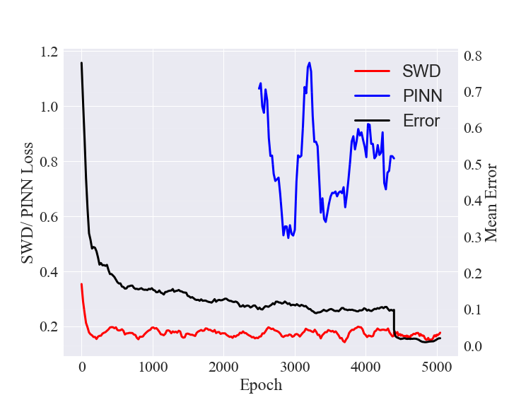
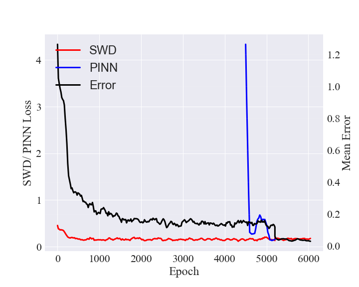
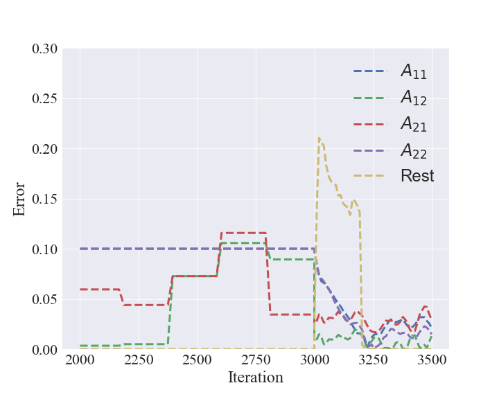
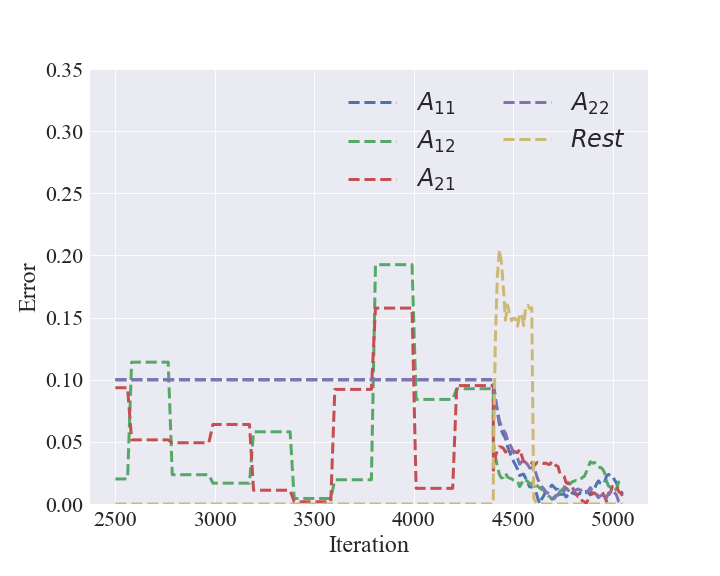
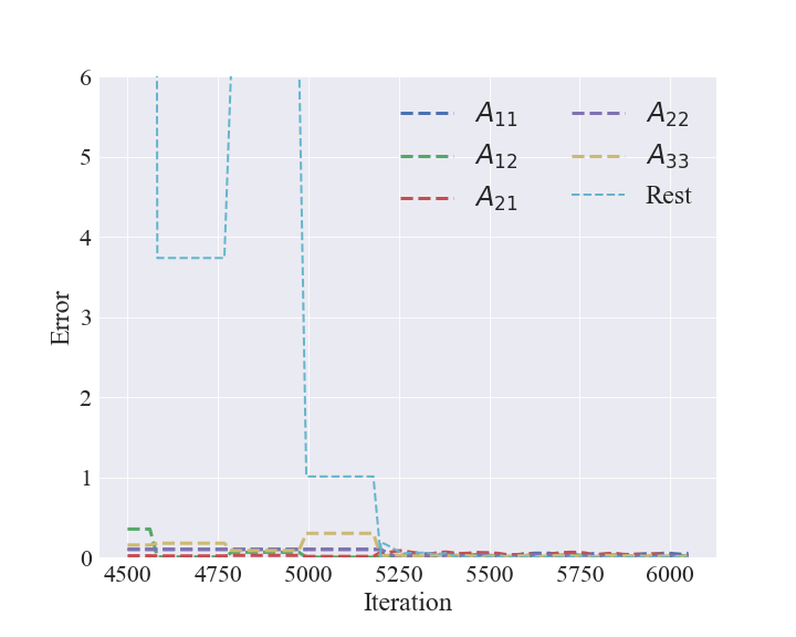
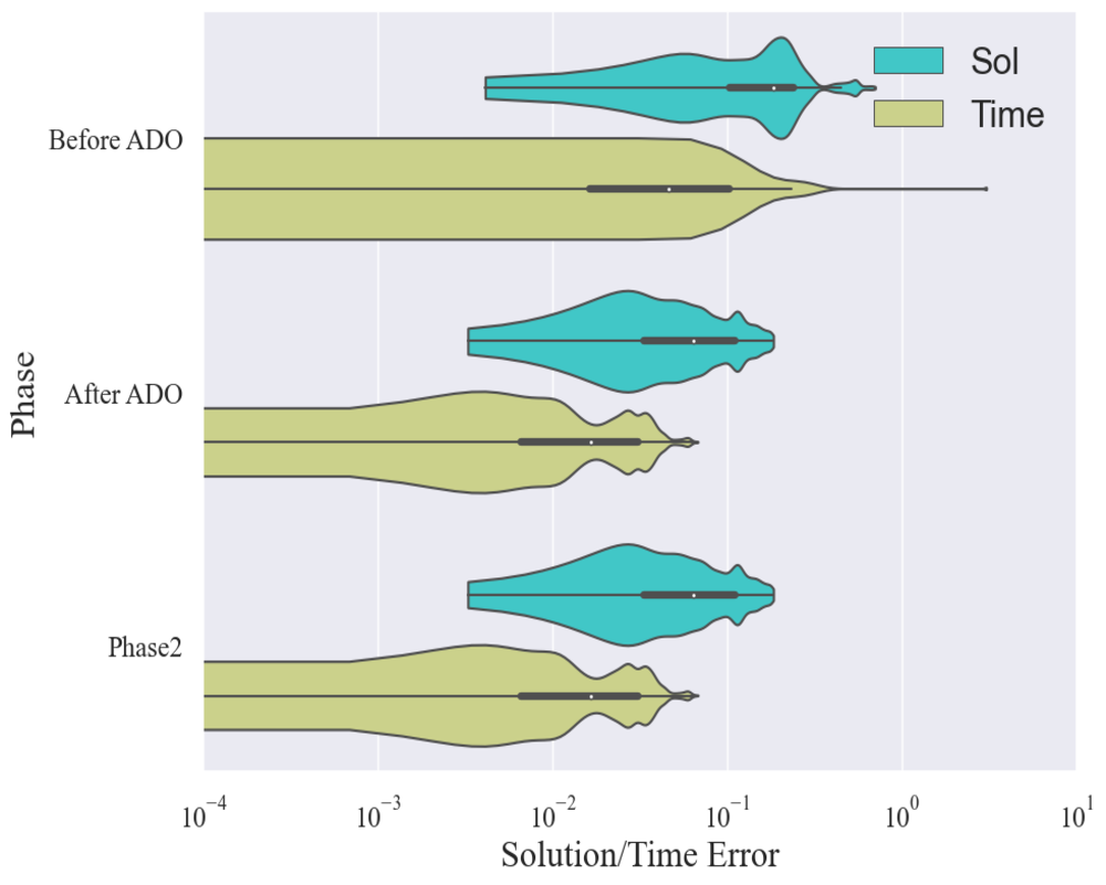
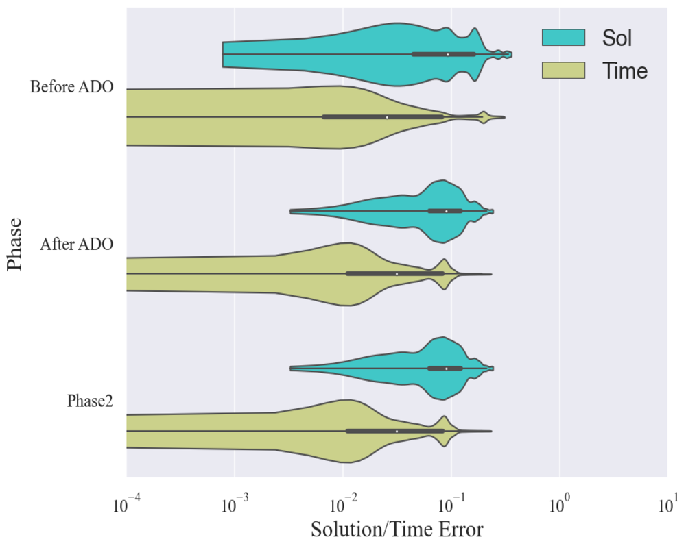
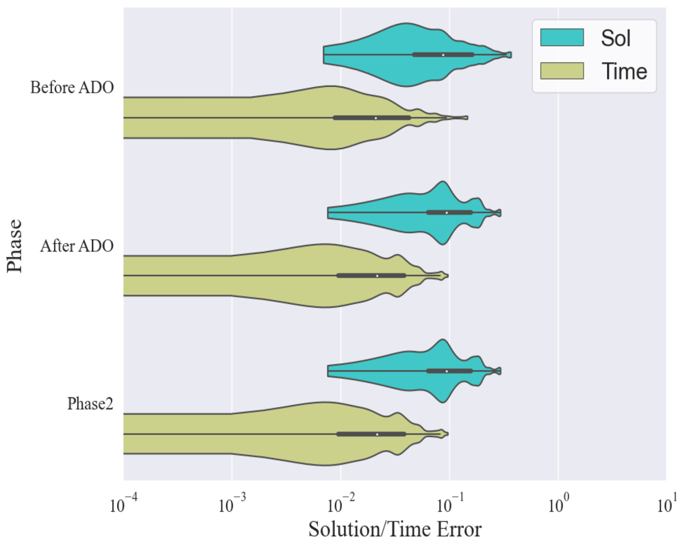
Figure 2: Reconstruction result of illustrative system:(a)-(c)Comparison between learned curve at different stage and ground truth for all system;(d)-(f)Recorded SWD Loss, PINN Loss and Average Error for all system;(g)-(i) The error curve of parameters and the sum of unexisting terms for all system;(j)-(l)The absolute error of learned solution evaluated at uniform grid and the absolute error of reconstructed time label of the dataset.

Settings	$||\boldsymbol{\mathbb{X}}||_{rms}$	RMAE	$\boldsymbol{E}_{para}$	$\boldsymbol{E}_{time}$	Reconstruct $A$
Linear2D	1.26	8.4$\%$,1.4$\%$	7.7$\%$,1.9$\%$	0.39$\%$ 0.056$\%$	$\begin{bmatrix}-0.12&-2.01\\ 1.97&-0.08\end{bmatrix}$
Cubic2D	1.13	7.0$\%$,0.6$\%$	9.2$\%$,0.8$\%$	0.9$\%$ 0.4$\%$	$\begin{bmatrix}-0.11&-2.02\\ 1.99&-0.99\end{bmatrix}$
Linear3D	1.31	5.7$\%$,1.5$\%$	6.8$\%$,3.0$\%$	0.53$\%$ 0.13$\%$	$\begin{bmatrix}-0.15&-2.01&0\\ 1.97&-0.07&0\\ 0&0&-2.8\end{bmatrix}$

Table 1: The results of illustrative examples.For the three metrics, the first one is computed using learned neural solution in Phase 1 while the second is computed by the solution of the learned ODE system .

5.3 Benchmark Examples

In the instances delineated below, we execute our algorithm on a selection of challenging ODE system derived from real-world models.

1. Lorenz equations represent a early mathematical model for characterizing atmospheric turbulence.This system exhibits chaotic behavior over the long time horizon, resulting in intricate intersecting trajectories and convoluted spiraling within the phase space

2. The Lotka-Volterra (LV) equations depict the dynamics of prey and predator populations in natural ecosystems and have found applications in real-world systems such as disease control and pollution management. In this study, we couple two independent LV equations(LV4D) to evaluate the efficacy of our algorithm in addressing high-dimensional problems.

3. The Duffing oscillator serves as a model for specific damped and driven oscillators, demonstrating long-term chaotic behavior.

Name	ODE	Parameters
Lorenz	$\left\{\begin{array}[]{l}\frac{dx_{1}}{dt}=\sigma(x_{2}-x_{1})\\ \frac{dx_{2}}{dt}=x_{1}(\rho-x_{3})-x_{2}\\ \frac{dx_{3}}{dt}=x_{1}x_{2}-\beta x_{3}\end{array}\right.$	$T=3$ $[\sigma,\rho,\beta]=[10,28,\frac{8}{3}]$ $\boldsymbol{x_{0}}=(10,-10,20)^{\top}$
Lotka-Volterra4D	$\left\{\begin{array}[]{l}\frac{dx_{1}}{dt}=\alpha_{1}x_{1}-\beta_{1}x_{1}x_{2}\\ \frac{dx_{2}}{dt}=\beta_{1}x_{1}x_{2}-2\alpha_{1}x_{2}\\ \frac{dx_{3}}{dt}=\alpha_{2}x_{3}-\beta_{2}x_{3}x_{4}\\ \frac{dx_{4}}{dt}=\beta_{2}x_{3}x_{4}-2\alpha_{2}x_{4}\end{array}\right.$	$T=11$ $[\alpha_{1},\alpha_{2},\beta_{1},\beta_{2}]=[1,1,3,5]$ $\boldsymbol{x_{0}}=(1,2,2,0.5)^{\top}$
Duffing	$\left\{\begin{array}[]{l}\frac{dx_{1}}{dt}=\alpha x_{2}\\ \frac{dx_{2}}{dt}=-\gamma x_{1}-\rho x_{2}-\beta x_{1}^{3}\end{array}\right.$	$T=11$ $[\alpha,\gamma,\rho,\beta]=[1,0.1,0.2,1]$ $\boldsymbol{x_{0}}=(0,2)^{\top}$

Table 2: Specifications of ODE examples.

As demonstrated in Table 3 and Fig3, our approach consistently attains precise performance across all three benchmarks, covering both chaotic and high-dimensional systems, thereby justifying versatility of our method with respect to diverse ODEs. In general, our method reconstructs the solution function with an RMAE of less than $5\%$ and the temporal label with less than $0.7\%$ after the Distribution Matching Phase in a noise-free environment. The reconstruction quality is further enhanced during the Parameter Identification Phase, wherein all active terms are successfully identified with an RMAE of less than $8\%$. We again observe that the solution and temporal labels exhibit similar accuracy to those obtained in the Distribution Matching Phase, thereby highlighting the efficacy of our approach. It should be noted that the reconstruction error for the solution and temporal label may remain high within some intervals when two trajectory pieces are close, despite the accurate identification of the model. This phenomenon can be observed in Fig3(a)-(c) for the Lorenz system and LV4D system, whose trajectories nearly coincide at distinct intervals.

To illustrate the precision, we compare our method with Principal Curve method, a traditional manifold parametrization method in the time label reconstruction task. We use the index provided by Principal Curve algorithm [cite T.Hastie] as the reconstructed time label. Indeed, we apply Principal Curve on the segmented trajectory piece and assign the estimated initial condition as the start points of each curve. The output indexes of each data point are normalized to $[T_{l},T_{l+1}]$ for $\mathbb{X}_{l}$. The result shows that given the same segmentation condition, our method is more than 30 times less than traditional Principal Curve method, while the Principal Curve fails to provide inter-interval resolution of time label. This problem is partly rooted in the parametrization principle of Principal Curve algorithm. It assign index based on the Euclidean distance between points, which often mismatch the velocity of curve determined by the observation distribution.

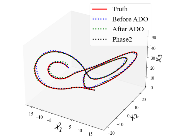
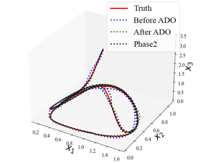
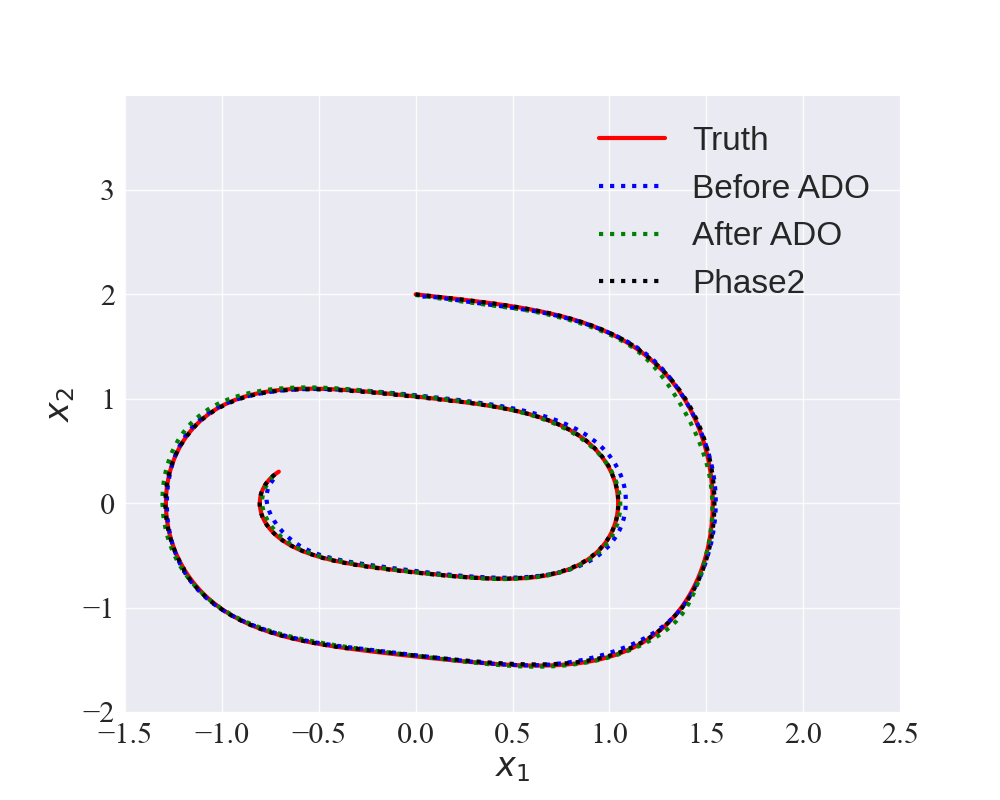
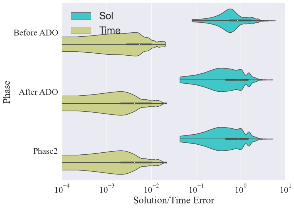
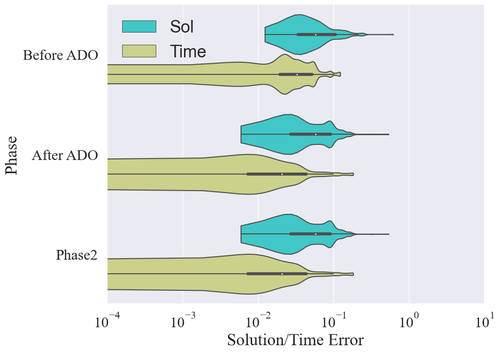
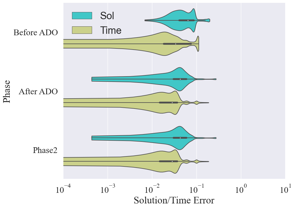
Figure 3: Reconstructing trajectories of four systems at different training stage:(a)Lorenz system;(b) LV4D system, plot the curve of first 3 dimension;(c) Duffing system;(d) Pendulum system. The learned trajectories before/after ADO and after Phase 2 is compared with the ground truth.

Settings	$||\boldsymbol{\mathbb{X}}||_{rms}$	RMAE	$\boldsymbol{E}_{para}$	$\boldsymbol{E}_{time}$	Parameters
Lorenz	25.36	2.8$\%$,1.5$\%$	0.65$\%$,0.58$\%$	0.40$\%$,0.10$\%$,25.9$\%$	$\begin{bmatrix}\sigma\\ \rho\\ \beta\end{bmatrix}=\begin{bmatrix}9.94\\ 27.89\\ 2.59\end{bmatrix}$
LV4D	1.12	4.2$\%$,2.3$\%$	5.6$\%$,4.3$\%$	0.69$\%$,0.31$\%$,13.0$\%$	$\begin{bmatrix}\alpha_{1}\\ \alpha_{2}\\ \beta_{1}\\ \beta_{2}\end{bmatrix}=\begin{bmatrix}0.97\\ 0.98\\ 2.93\\ 4.65\end{bmatrix}$
Duffing	1.17	3.88$\%$,1.63$\%$	8.53$\%$,2.03$\%$	0.30$\%$,0.20$\%$,19.4$\%$	$\begin{bmatrix}\alpha\\ \gamma\\ \rho\\ \beta\\ \end{bmatrix}=\begin{bmatrix}0.99\\ 0\\ 0.21\\ 1.06\end{bmatrix}$

Table 3: The results of benchmark examples.For the three metrics, the first results is computed using learned neural solution in Phase 1 while the second is computed by the solution of the learned ODE system. For the $\boldsymbol{E}_{time}$ column, the third results is computed by traditional Principal Curve method.All the inactive terms in library are successfully removed during training in four experiment, so the Parameters row describes the identified systems.

5.4 Noisy data

Here we want to investigate the effect of noise on system identification. To this end, a noise ratio $\sigma_{NR}$ is specified, and the observation data is blurred by

(13) $$\hat{\boldsymbol{\mathbb{X}}}=\boldsymbol{\mathbb{X}}+\epsilon$$

where $\boldsymbol{\mathbb{X}}$ is the simulated noise-free observation and $\epsilon$ is the white noise with variance $\sigma^{2}$, where

(14) $$\sigma=\sigma_{NR}\times||\boldsymbol{\mathbb{X}}||_{rms}=\sigma_{NR}\times\frac{1}{n}\sum_{i=1}^{n}\left(\sum_{j=1}^{d}\boldsymbol{x_{i,j}}^{2}\right)^{\frac{1}{2}}$$

Besides the single trajectory setting we used above, we also present the results on observation of multiple short trajectories which can be viewed as the segmentation of a long trajectory with noise-free initial conditions. In this setting we don’t do trajectory segmentation anymore. We exam the robustness again on the four benchmark systems for $1\%$,$3\%$ noise in single trajectory setting and $3\%$,$5\%$ noise in multiple trajectory setting. The three evaluation metric are summarized in Fig4 for different setting.

As can be observed from the results, the reconstruction error of solution and time generally increases as the noise level increases. The major challenge is when the noise level are large, the trajectory may overlaps and causes error in trajectory segmentation. If a cluster have two disjoint pieces with different initial point, the single trajectory condition is no longer established. When it comes to multiple short trajectories, our method is still effective to capture the hidden dynamic precisely even with large noise level. Further more, the result shows that the non-polynomial terms introduce extra difficulty in both parameter identification and solution reconstruction for data with large noise level. However, with the help of Parameter Identification Phase, we still obtained high-quality results.

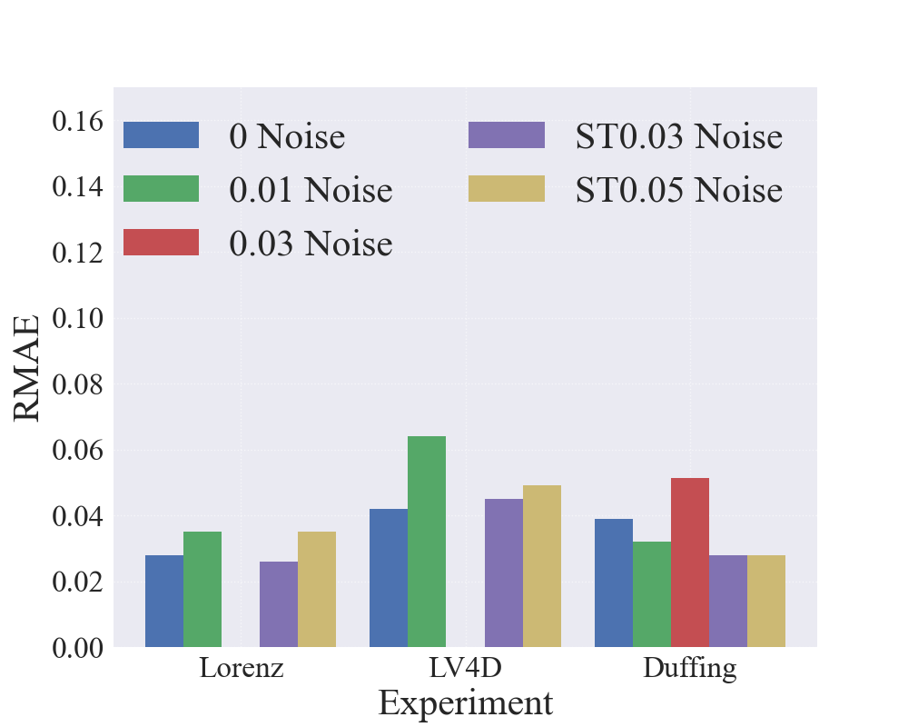
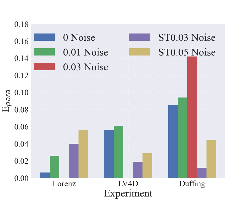
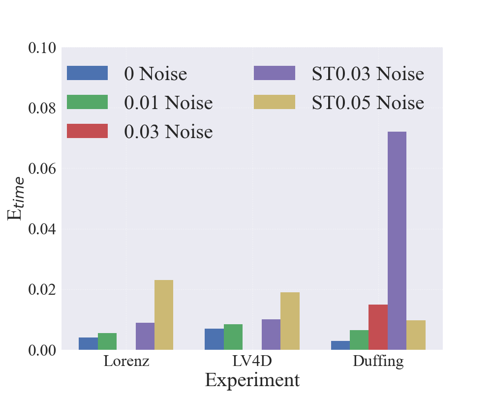
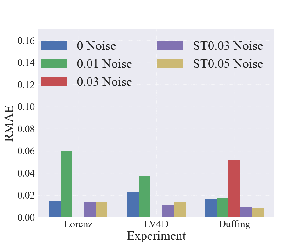
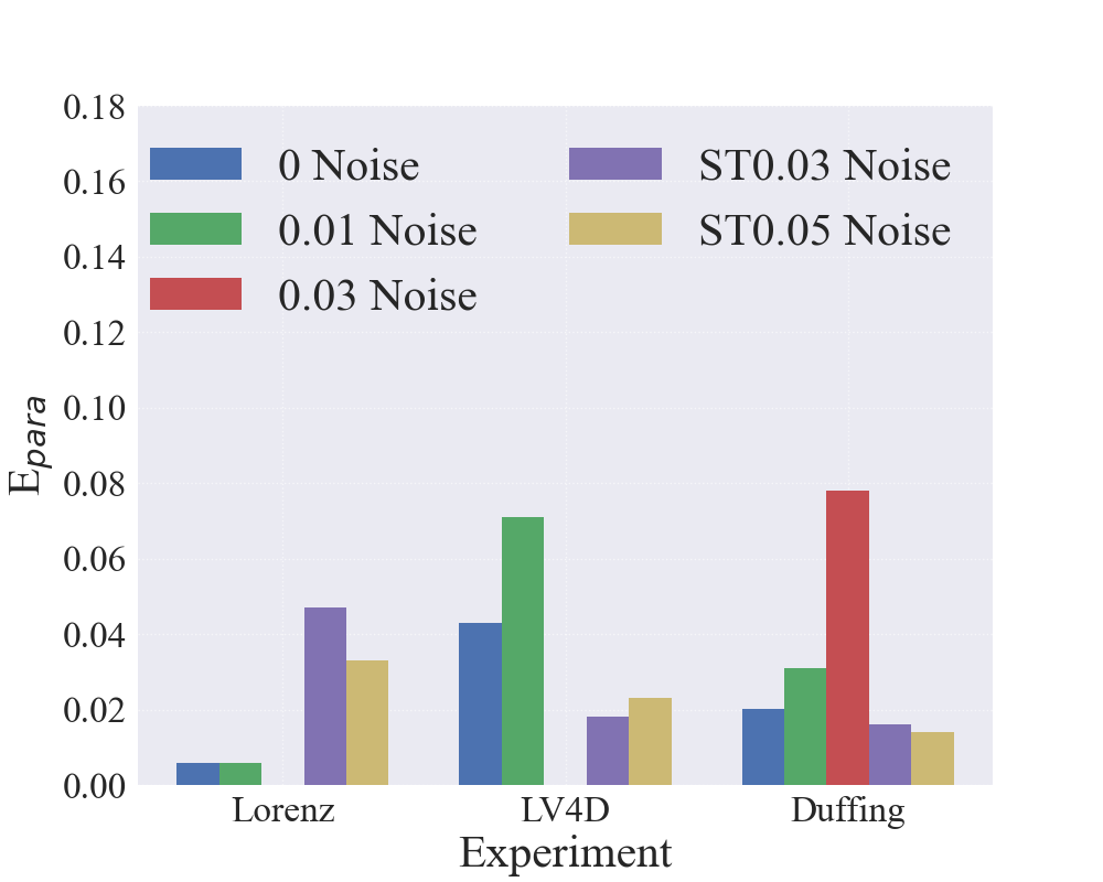
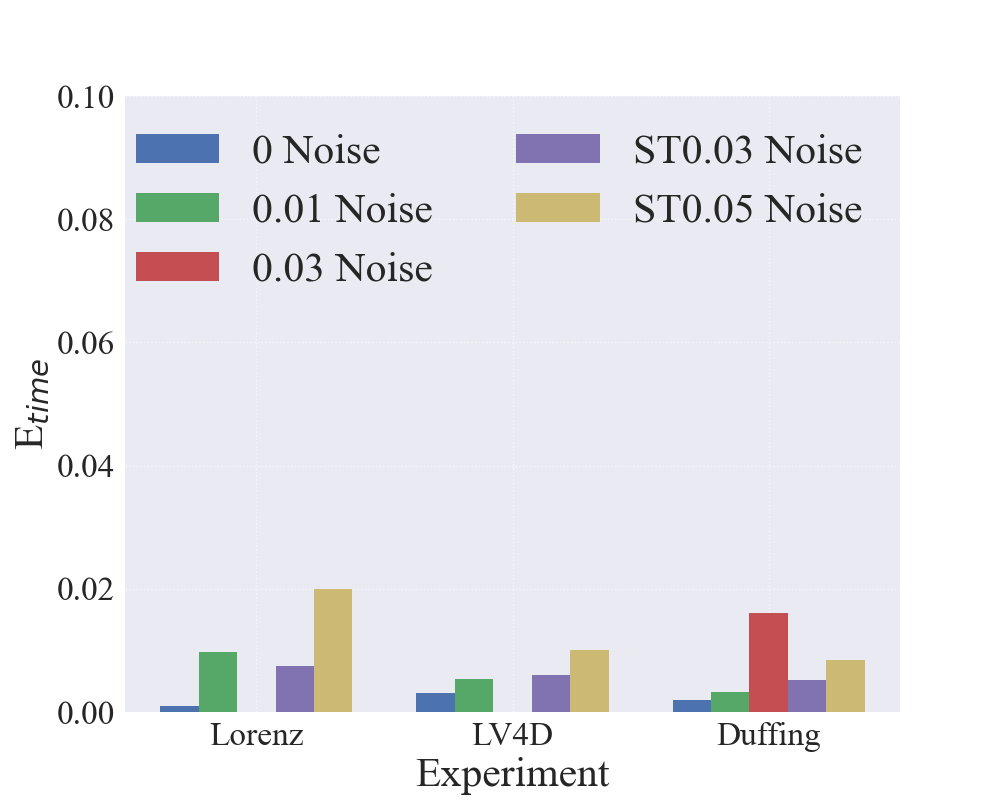
Figure 4: Evaluation of reconstruction results from noisy data in two trajectory type and four systems.(a)-(c):The RMAE of learned solution, identified parameters and reconstructed time labels in Phase1; (d)-(f):The RMAE of learned solution, identified parameters and reconstructed time labels in Phase2. The data of Lorenz and LV4D systems for $3\%$ noise is missing because the segmentation step failed to provide non-overlapping trajectory pieces.

5.5 General Hamiltonian system out of basis

One may have doubts about the restricted basis expansion in this framework, as the dynamical system with real-world backgrounds may not necessarily be representable by a finite set of basis functions. In this subsection, we exam the approximation capability of our method by the famous Pendulum system:

(15) $$\left\{\begin{array}[]{l}\frac{dx_{1}}{dt}=\alpha x_{2}\\ \frac{dx_{2}}{dt}=\beta\sin(x_{1})\\ \end{array}\right.$$

where the initial condition is $\boldsymbol{x_{0}}=(1,0.1)^{\top}$, the time length is $T=8$ and the parameters are $[\alpha,\beta]=[1,1]$. In this case, the Hamiltonian $H(x_{1},x_{2})=\frac{1}{2}x_{2}^{2}+\cos(x_{1})$ is a conserved quantity describing the total energy of a Hamiltonian system.

We first utilize our method in a larger basis

$$\mathbf{\phi}_{1}=\{Poly(3),\sin(x_{1}),\sin(x_{2}),\cos(x_{1}),\cos(x_{2})\}$$

that contains all the existing terms in the pendulum system and a smaller 3rd order complete polynomials library $\mathbf{\phi}_{2}=\{Poly(3)\}$. Here observations with five different noise level are considered to provide a more comprehensive view.

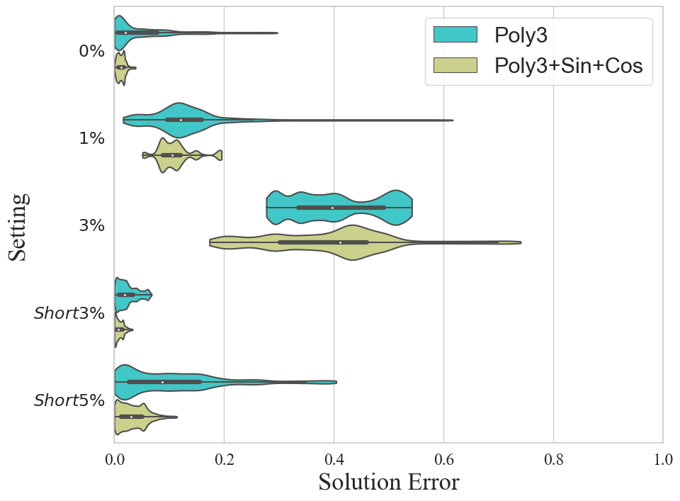
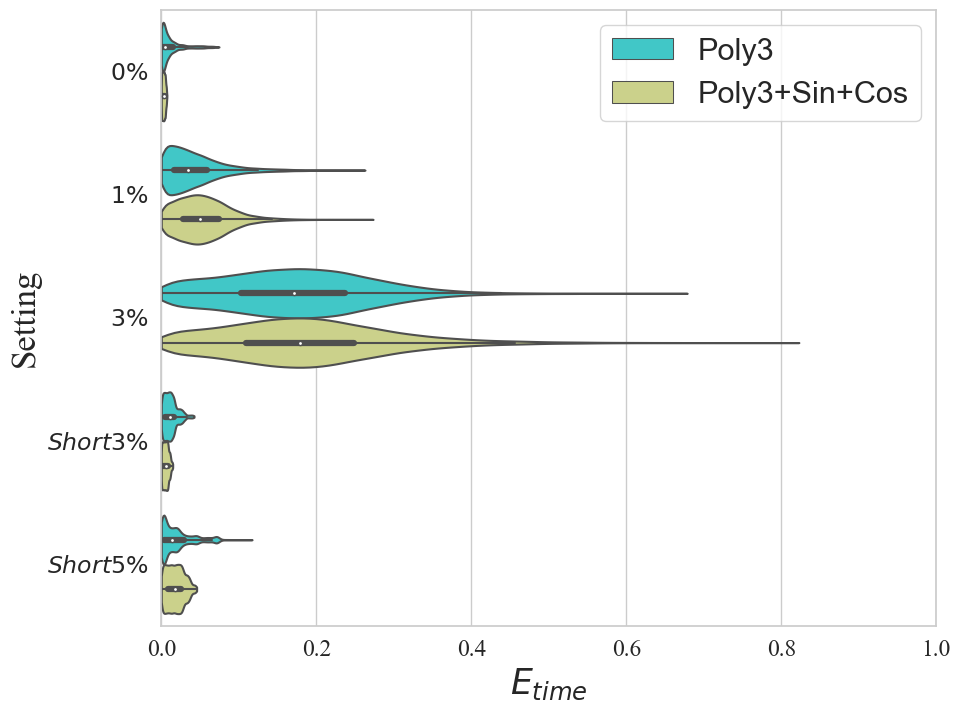
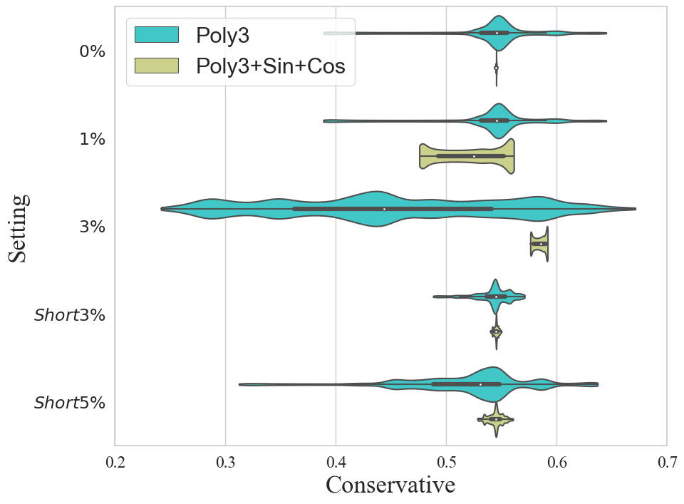
Figure 5: Reconstruction result of Pendulum system:(a)Violin plot of absolute error of learned solution function for two basis setting in 5 different noise level;(b)Violin plot of absolute error of reconstructed temporal label for two basis setting in 5 different noise level;(c)Voilin plot of Hamiltonian of learned dynamical system in Phase2

The result obtained from Fig6 demonstrates that the learned dynamical system with a general polynomial basis $\mathbf{\phi}_{2}$ reaches high precision in the reconstruction of solution function($1.2\%$RMAE for noise free setting) and temporal label($0.07\%$RMAE for noise free setting), yet slightly lower than the result of larger basis $\mathbf{\phi}_{1}$($0.28\%$RMAE for solution function and $0.07\%$RMAE for temporal label) . However, the Hamiltonian along the learned trajectory of the restricted basis have significant larger variance than that of $\mathbf{\phi}_{1}$, especially for large noise level. This is reasonable since with larger library the algorithm successfully identifies the exact components that form the conservative system, while the polynomial system does not inhibit the Hamiltonian structured, though approximated in the solution function perspective.

To investigate in the approximation capability of our method with respect to the scale of library, we approximate the source term using polynomial basis functions of 5 different orders. We compare the absolute error of solution function and the temporal labels for different basis in Fig6. As the order of polynomial basis from 1 increases to 4, the results obtained by our method gradually approach the ground truth, and the best learning performance is achieved when the order is 4, with $0.44\%$ RMAE of solution and $0.08\%$ RMAE of temporal label. For $Poly(5)$ basis, the sparse regression failed to provide a convergent estimation of dynamical system on account of the increasing sensitivity of higher order parameters, while in Phase2 numerical instability of forward solver causes difficulties for parameter identification since our sampled temporal label isn’t uniform. This results in the growth of solution error and temporal label error.

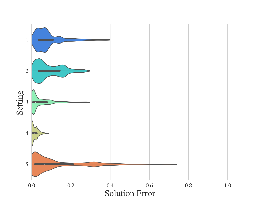
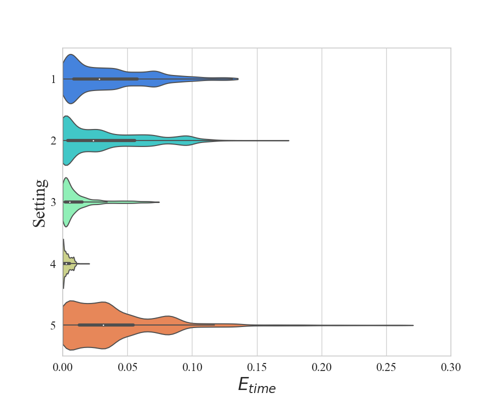
Figure 6: Reconstruction result of Pendulum system using polynomial basis with different order:(a)Absolute error of solution parametrized by different order of polynomial basis;(b)Absolute error of temporal label parametrized by different order of polynomial basis.

5.6 Different observation distribution

We further investigate the robustness of our method for data with different observation distribution. Here we truncate the normal distribution $\mathcal{N}\left(\frac{T}{2},\left(\frac{T}{3}\right)^{2}\right)$ in $[0,T]$ and treat it as the observation distribution. The results of four benchmark systems are shown in Fig7 and Table4. Overall, our method presents a stable performance w.r.t different observation distribution for reconstructing the solution and time label.

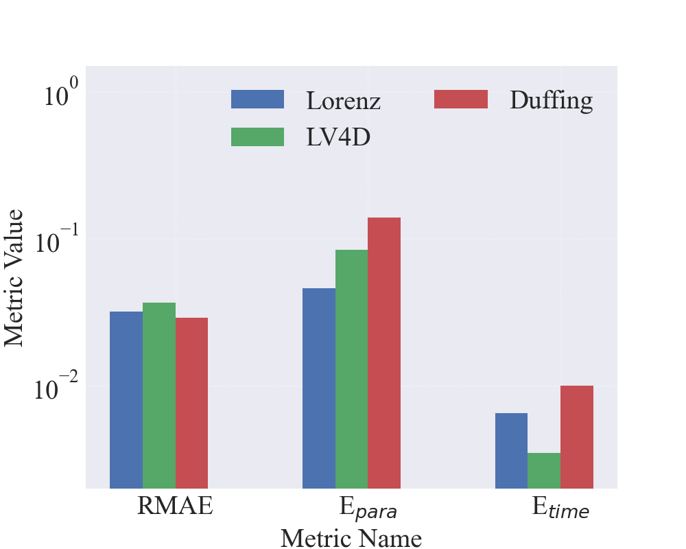
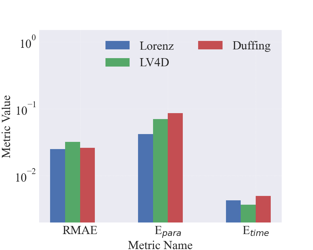
Figure 7: Evaluation of reconstruction results from data with truncated normal distribution of observation time.(a):The evaluation metrics of reconstruction results in Phase1;(b):The evaluation metrics of reconstruction results in Phase2

Settings	RMAE	$\boldsymbol{E}_{para}$	$\boldsymbol{E}_{time}$
Lorenz	3.2$\%$,2.5$\%$	4.6$\%$,4.2$\%$	0.65$\%$,0.43$\%$
LV4D	3.7$\%$,3.2$\%$	8.4$\%$,7.0$\%$	0.35$\%$ 0.37$\%$
Duffing	2.9$\%$,2.6$\%$	14.0$\%$,8.6$\%$	1.0$\%$ 0.50$\%$

Table 4: The results of benchmark examples with truncated normal distribution of observation time. For the three metrics, the first one is computed using learned neural solution in Phase 1 while the second is computed by the solution of the learned ODE system.

6 Conclusion and future Work

Point cloud data lacking time labels is a common data type for scientific research. Unveiling the hidden dynamics and reconstructing the missing temporal label is helpful for understanding the physical laws behind the observation. In this study, we assume that the observation time instants is sampled from a known distribution and the observation data are generated by a ODE system with perturbation.and formulate the reconstruction into a rigorous minimization problems with respect to a continuous transformation of random variable. We perform theoretical analysis of the uniqueness of smooth transformation given the distribution of observation data and time instants under certain conditions.

In computational perspective, we propose a two-phase learning algorithm to simultaneous estimate the potential trajectory and the hidden dynamical system. In Distributional Matching phase, we leverage the Sliced Wasserstein Distance to construct a neural network approximation of the data trajectory and utilize Alternating Direction Optimization technique to distill sparse parameter estimation of the ODE system from a large expression library. In Parameter Identification Phase, we adopt the Neural ODE paradigm to further refine the estimation. Based on the empirical observation that complex trajectory renders higher non-convexity and numerical issue for the learning task, we leverage the manifold hypothesis to propose a clustering based partition algorithm to transform long trajectory in to short trajectory segments before training.

On the experimental side, We demonstrate our method on a number of illustrative and complex dynamical systems exhibiting challenging characteristic (e.g., chaotic, high-dimensional, nonlinear).Results highlight that the approach is capable of uncovering the hidden dynamics of the real-world point cloud data, and reconstruct the temporal label in high accuracy. The proposed method maintains satisfactory robustness against different types of distribution of observation time instant (Uniform and truncated Gaussian) and high level noises when multiple short trajectories are provided, while in single trajectory setting the perturbation bring about overlapping and lead to failure in trajectory segmentation and temporal label reconstruction. Results show that the approximation capability is increasing as the library is enlarging, obtaining finer reconstruction of solution function and temporal label. However, including high-order terms in the library may introduce numerical instability in the forward computation and the regression process.

As part of the future work, we will try the proposed framework on more challenging regime. For example, one of the important directions is to unveiling physical laws from PDE-driven or SDE-driven observation without temporal label. Another interesting direction which is worth exploring is to embed more statistical insight in the algorithm to enhance the robustness for highly perturbed data.

Appendix A Proof of Theorem 2.1

To prove the theorem, we introduce the following assumption    

1. The probability density function(PDF) $p(t)$ of observation time instant $t$ supports on a finite interval $[0,T]$ and satisfies $p(t)\in C([0,T]),p(t)>0$ for all $t\in[0,T]$, and we denote the space of satisfied observation distribution as $\mathcal{T}$, and the space of cumulative distribution function(CDF) of distributions in $\mathcal{T}$ as $\mathcal{P}$.

2. The dynamical system $\boldsymbol{x}(t)\in\mathcal{C}$, and the time derivative of $\boldsymbol{x}(t)$ have positive norm.

 

We consider that curves with different speed are the same and introduce a equivalence relation in $\mathcal{C}$

Definition A.1.

,,, $r_{1}\in\mathcal{C}:[0,T_{1}]\rightarrow[0,1]^{d},r_{2}\in\mathcal{C}:[0,T_{2}]\rightarrow[0,1]^{d}$ are equivalent if there exists an $C^{1}$ strictly increasing map $s:[0,T_{1}]\rightarrow[0,T_{2}]$ , such that $r_{1}=r_{2}\circ s$, which we denoted as $r_{1}\sim r_{2}$.

We remark that the $s$ can be viewed as a change of velocity for the curve.

The following lemma shows the existence of a representator with unit speed for each equivalence class

Lemma A.2.

For all $r\in\mathcal{C}:[0,T_{1}]\rightarrow[0,1]^{d}$, there exists an unique $C^{1}$ strictly increasing map $s:[0,T_{1}]\rightarrow[0,T_{2}]$ such that $p=r\circ s,\|\frac{dp}{dt}(t)\|_{2}\equiv 1.$

Proof A.3.

By Chain rule, $\frac{dp}{dt}=r^{\prime}\circ s(t)s^{\prime}(t)$, then we have

(16) $$\|\frac{dp}{dt}(t)\|_{2}=\|r^{\prime}\circ s(t)\|_{2}s^{\prime}(t),$$

The desire $s$ is obtained by solving the ODE for $[0,T_{2}]$

(17) $$\left\{\begin{array}[]{c}s^{\prime}(t)=\frac{1}{\|r^{\prime}\circ s(t)\|}\\ s(0)=0.\end{array}\right.$$

The global existence and uniqueness of $s$ is guarantee by the Existence and Uniqueness theorem for ODE. The regularity of $s$ is given by the fact that $r\in C^{1}$.

Lemma A.4.

Let $r\in\mathcal{C}:[0,T]\rightarrow[0,1]^{d}$ be an injective $C^{1}$ curve with $\|r^{\prime}(t)\|\equiv 1,$ then for any curve $\tilde{r}\in\mathcal{C}:[0,T_{1}]\rightarrow[0,1]^{d}$ for some $T_{1}$ with $\|\tilde{r}^{\prime}(t)\|\equiv 1$ such that $\tilde{r}(0)=r(0),\{r(t)|t\in[0,T]\}=\{\tilde{r}(t)|t\in[0,T_{1}]\}$,$\tilde{r}\sim r$.

Proof A.5.

Suppose there exists such $\tilde{r}(t)$ that satisfies the aforementioned condition and is not equivalent to $r$.

First, it’s easy to conclude that $T_{1}=T$ by the arc length formula since $\|\tilde{r}^{\prime}(t)\|\equiv\|r^{\prime}(t)\|\equiv 1$.

Since $\tilde{r}\not\sim r$, there exists $t_{0}\in(0,T]s.t.r(t_{0})\neq\tilde{r}(t_{0})$. Consider the set $S=\{t\in[0,T]|r(t)\neq\tilde{r}(t)\}$, $S$ is not empty and thus $t_{1}:=\inf(S)\in[0,T]$ exists. We claim that there exists $t_{2}\neq t_{1},r(t_{2})=r(t_{1})$, which leads to contradiction since $r$ is injective.

Indeed, by $r(t_{1})=\tilde{r}(t_{1})$, we consider the extend curves from $t_{1}$. Let $S_{1}^{\Delta t}=\{r(t_{1}+t)|t\in(0,\Delta t]\},S_{2}^{\Delta t}=\{\tilde{r}(t_{1}+t)|t\in(0,\Delta t]\}$, we claim that there exists $\Delta t>0$ such that $S_{1}^{\Delta t}\cap S_{2}^{\Delta t}=\emptyset$.

If our claim holds, then there exists $U\subset[0,T]$, such that $\{r(t)|t\in U\}=S_{2}^{\Delta t}$. We can find an series $\{\tilde{r}(\tilde{t}_{i})\}_{i=1}^{+\infty}$ in $S_{2}^{\Delta t}$ converges to $\tilde{r}(t_{1})$, thus the corresponding series $\{r(\tilde{t}^{\prime}_{i})\}_{i=1}^{+\infty}$ converges to $\tilde{r}(t_{1})$ too. We then conclude that $\lim_{n\rightarrow\infty}\tilde{t}^{\prime}_{i}=t_{2}\neq t_{1},r(t_{2})=r(t_{1})$ via a subsequence argument.

Now we proof the second claim, again we use proof by contracdiction. Suppose for any $\Delta t>0,S_{1}^{\Delta t}\cap S_{2}^{\Delta t}\neq\emptyset$, then $r(t)$ and $\tilde{r}(t)$ must coincide in $[t_{1},t_{1}+\Delta t_{1}]$ for small $\Delta t_{1}>0$ since $\|r^{\prime}(t)\|\equiv\|\tilde{r}(t)\|\equiv 1$ which contradicts to the fact that $t_{1}=\inf\{t\in[0,1]|r(t)\neq\tilde{r}(t)\}$.

Return to our setting, utilizing the lemma we prove the uniqueness theorem of our inverse problem

Proof A.6.

Given $\mathbb{X}$ and $\mathbf{x}_{0}$, by theorem2.1 we determine the dynamical system up to a strictly increasing coordinate transformation denoted by $[r(\cdot)]$, where $r(\cdot)$ is the smooth curve with unit speed

$$\left\{\begin{array}[]{cl}\{r(t)|t\in[0,T_{1}]\}&=Img(\mathbb{X})\\ r(0)&=\mathbf{x}_{0}\\ \|\frac{dr}{dt}\|_{2}&=1,\forall t\in[0,T]\\ \end{array},\right.$$

where $T_{1}$ is the arclength of the trajectory in phase space and $Img(\mathbb{X})$ is the range of $\mathbb{X}$ as a random vector. Thus $r^{-1}(\mathbb{X})$ is a random variable with $C^{1}$ CDF $\tilde{P}(\cdot)$. The desire transformation is provided by its inverse explicitly

(18) $$\begin{array}[]{cccl}\mathbf{x}^{-1}:&Img(\mathbb{X})&\rightarrow&[0,T]\\ &\hat{\mathbf{x}}&\rightarrow&P^{-1}\circ\tilde{P}\circ r^{-1}(\hat{\mathbf{x}})\end{array},$$

by assumption the inverse map is $C^{1}$ and injective.

A.1 Restriction of Neural ODE

To identify the hidden dynamics using data without temporal label, a direct way is to transform the problem into a Neural ODE regression task with random collocations. To establish the above idea, in each epoch, we first sample $t_{1}<t_{2}<\ldots<t_{B}$ in $(t_{0},t_{0}+T)$ from $p_{t_{0}}$ and $\{\boldsymbol{x_{i}}\}_{i=1}^{B}$ uniformly from dataset $\mathbb{X}$. Then we solve the initial value problem to obtain numerical solution on the sampled time instants $\{\boldsymbol{x}_{\boldsymbol{\theta}}(t_{i})\}_{i=1}^{B}$, where

$$\boldsymbol{x}_{\boldsymbol{\theta}}(t_{i})=\textit{ODESolve}\left(\boldsymbol{f}(\tilde{\boldsymbol{x}},\boldsymbol{\theta})),\boldsymbol{x}_{0},[0,t_{i}]\right).$$

In the current study, our primary focus lies in elucidating the underlying mechanism governing the data, thereby seeking to derive an explicit ordinary differential equation (ODE) model rather than employing a black-box neural network. Stemming from this perspective, we assume that the physical law is governed by a few important terms which can be identified from a comprehensive library of potential expressions, where the sparse regression can be applied. Such assumption leads to a reformulation of the dynamical system form

$$\frac{d\boldsymbol{x}}{\operatorname{dt}}=\boldsymbol{\phi}(\boldsymbol{x})\boldsymbol{\Lambda},$$

where $\boldsymbol{\phi}(\boldsymbol{x})\in\mathbb{R}^{1\times s}$ is an library of function expression consisting of many candidates, e.g., constant, multi-variable polynomial, exponential function, trigonometric terms, and $\boldsymbol{\Lambda}\in\mathbb{R}^{s\times d}$ is the weight matrix, thus $\boldsymbol{\theta}=\boldsymbol{\Lambda}$. To achieve a distribution matching target, we instead use Sliced Wasserstein Distance (6) as our loss function

(19) $$L_{SWD}=SW_{2}^{2}(\{\boldsymbol{x}_{\boldsymbol{\Lambda}}(t_{i})\}_{i=1}^{B},\{\boldsymbol{x_{i}}\}_{i=1}^{B}).$$

We update $\boldsymbol{\Lambda}$ via gradient descent and stop when the loss function is smaller then a threshold with final result $\boldsymbol{\Lambda}_{end}$.

Although Neural ODE have been successfully employed for regression tasks involving time-series data, it can sometimes have difficulty in learning distributions through trajectory. Initially, we found that, in some relatively long trajectory, whether the success of the learning approach is profoundly susceptible to the preliminary selection of parameters owing to periodic or intricate structures present within the phase space. To illustrate this notion more comprehensively, we depict the loss landscape around the ground truth of a simple ODEs:

$$\left\{\begin{array}[]{ll}\frac{dx_{1}}{dt}=-0.1x_{1}^{3}+2x_{2}^{3}\\ \frac{dx_{2}}{dt}=-2x_{1}^{3}-0.1x_{2}^{3}\\ \boldsymbol{x}(0)=(4,0)^{\top}.\end{array}\right.$$

where we observe the data with a uniform distribution $\boldsymbol{t}\sim\mathcal{U}(0,10)$. Here we assume that the library is optimally determined as $\{x_{1}^{3},x_{2}^{3}\}$ and the diagonal of the parameter matrix $A=\begin{bmatrix}-0.1&A_{12}\\ A_{21}&-0.1\\ \end{bmatrix}$ is given. We estimate the Sliced Wasserstein Distance of trajectories with parameters in the neighbourhood of the ground truth $[1,3]\times[-3,-1]$. As Fig8(b) shows that the loss function manifests a strong non-convexity, resulting in even proximate selections would get stuck in local minima like the dashed blue curve in Fig8(d) with improper learning rates. Nevertheless, the non-convexity can be substantially alleviated for a comparatively brief and uncomplicated trajectory. Fig8(c) exhibits a near-convex loss function in the identical parameter region for observation instances $\boldsymbol{t}\in[0,0.4]$. Such analysis suggest that partitioning intricate trajectory observations into abbreviated segments could diminish the complexity.

A potential concern arises when the forward process, responsible for generating synthetic samples, may exhibit considerable stiffness or other numerical challenges, such as divergence. Implementing a more precise and stable numerical scheme could alleviate this issue; however, it may also incur a substantial computational expense and is inadequate to overcome innate divergence of systems with erroneous parameters. We plot the contour map of the $\sup_{t\in[0,10]}||\boldsymbol{x_{t}}||_{2}$ in a large parameter space $\{(A_{12},A_{21})|(A_{12},A_{21})\in[-3,3]\times[-3,3]\}$ in 8(a), which shows that an initialization of parameters in the first or third quadrant results in blow up solution and prevent further update. The evolution of numerical ODE solver can be viewed as an auto-regressive model, which computational inefficient for long sequence rollout.

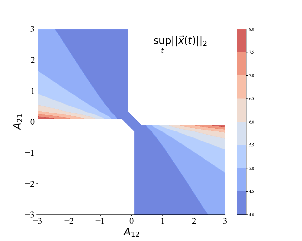
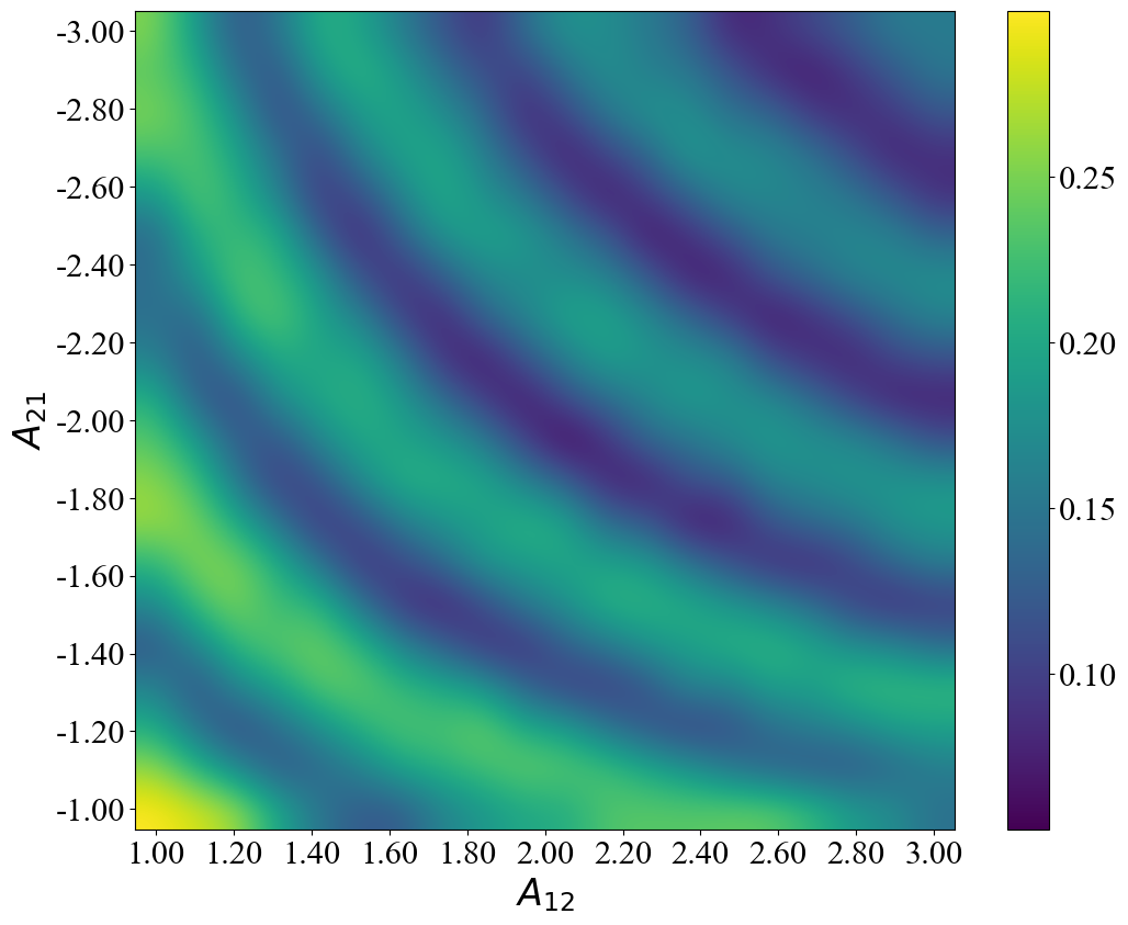
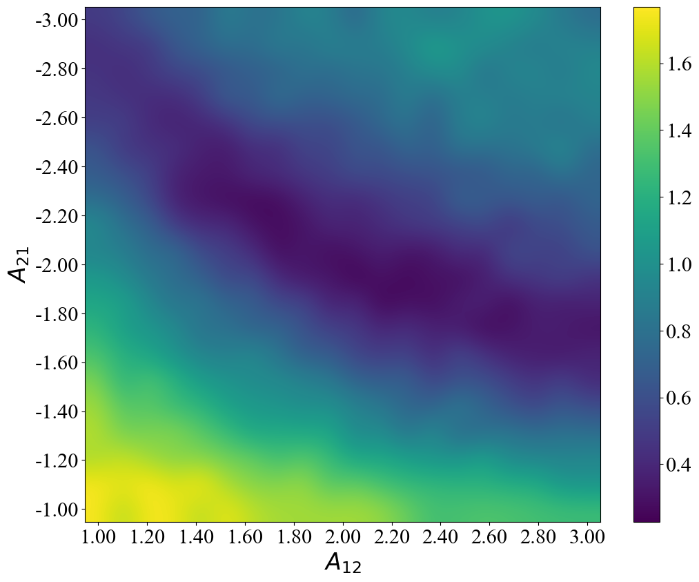
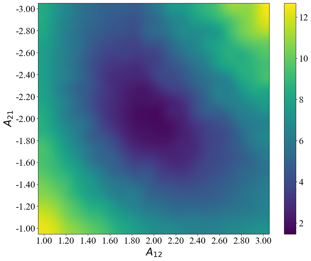
Figure 8: Loss landscape analysis of Cubilc2D problem: (a)The estimated $\sup_{t\in[0,10]}||\boldsymbol{x_{t}}||_{2}$ of each parameter choice in $[-3,3]\times[-3,3]$;(b) The SWD loss landscape of $A_{12},A_{21}$ in $[1,3]\times[-3,-1]$ with $T=10$;(c)The SWD loss landscape of $A_{12},A_{21}$ in $[1,3]\times[-3,-1]$ with $T=0.4$;(d).

Appendix B Verification of Wasserstein Distance Loss

In this paper, we employ the Sliced Wasserstein Distance to fast approximate the Wasserstein Distance between the generated data distribution and the observed distribution, and provide an update direction for each data point (derived from the gradient of the loss function). In this section, we consider the direct computation of the Wasserstein Distance and Optimal transportation matrix between the two empirical distributions, and based on this, we calculate the update direction for each data point to update the parameters in the neural network and the pa rametrized dynamical system. This serves to verify the feasibility of regression based on Wasserstein Distance. Specifically, we sample the observed data from trajectory segments and compute the generated solution data within the corresponding time interval by the neural network or numerical solver, yielding two point clouds $\{x_{i}\}_{i=1}^{n},\{y_{j}\}_{j=1}^{n}$. We set the mass of each point as $\frac{1}{n}$ and utilize the Sinkhorn algorithm to compute the Optimal transportation matrix between the two empirical distributions. The update direction for each generated data point is a weighted average of the direction vectors pointing from itself towards the points it was transported to. We calculate the update direction for each generated data point as the initial gradient for backpropagation and update the parameters using the AdamW method. We mention that the algorithm here is the same as the method in this paper, except for the gradient computation.

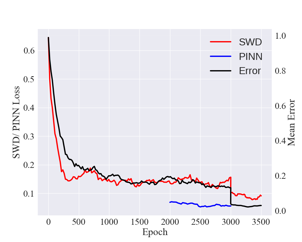
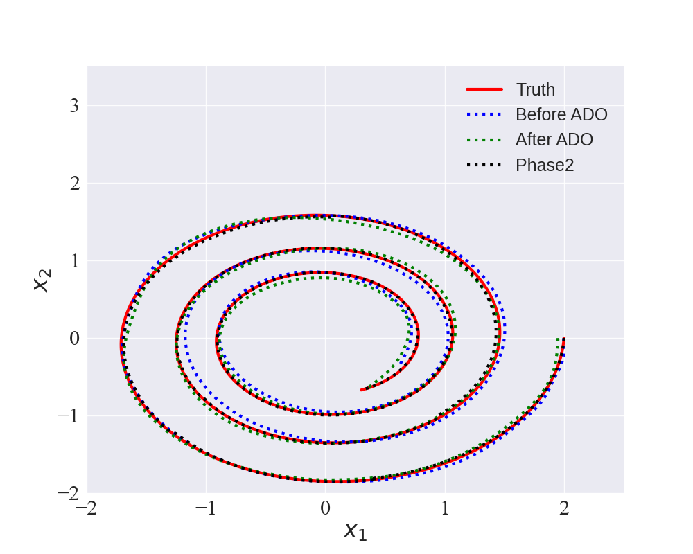
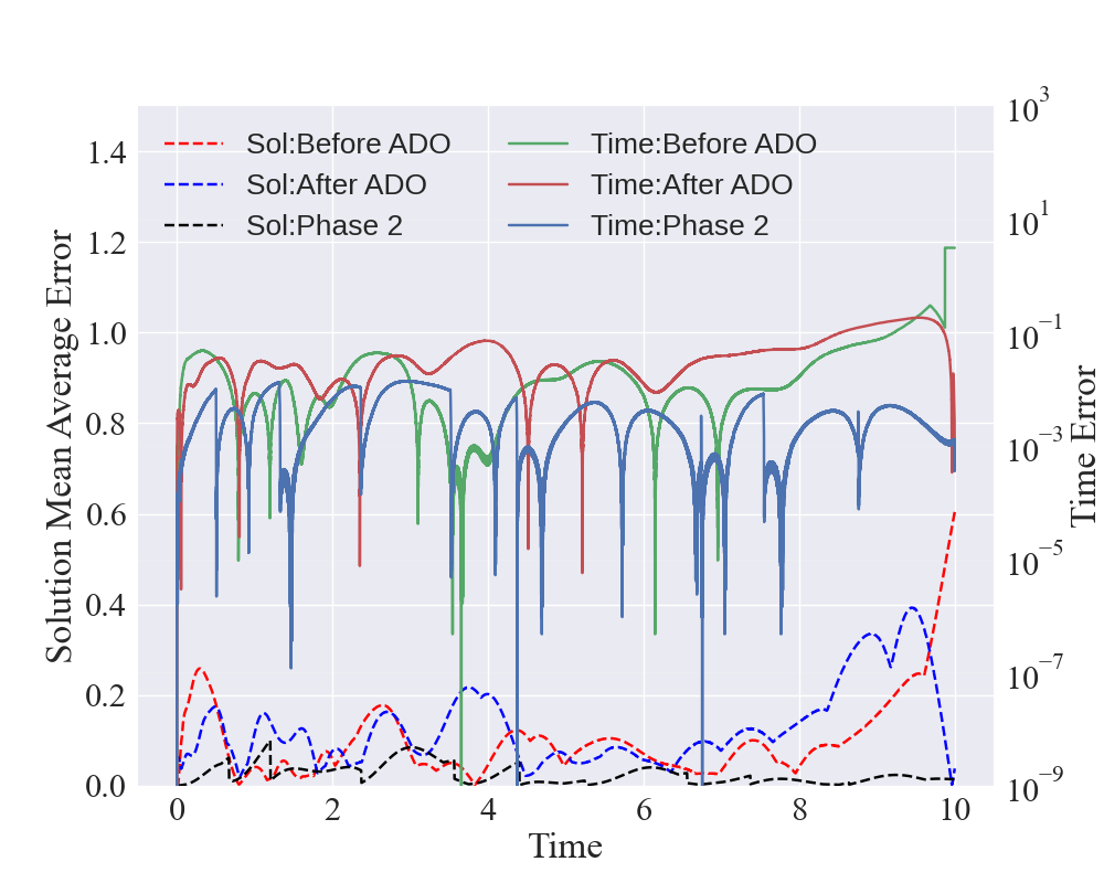
Figure 9: Evaluation of reconstruction results from

Appendix C Experiment Detail

Parameters	$n_{cluster}$	library	$\Lambda_{Threshold}$	$lr$	$\lambda_{init}$	$\lambda_{reg}$
Linear2D	10	Poly(3)+Exp	0.04	$3e-4$	0.5	$1e-3$
Cubic2D	10	Poly(3)+Exp	0.06	$6e-4$	0.5	$3e-5$
Linear3D	10	Poly(3)+Exp	0.04	$3e-4$	0.5	$1e-3$
Lorenz	10	Poly(3)+Exp	0.04	$3e-4$	0.5	$3e-5$
LV4D	10	Poly(2)+Exp	0.045	$6e-4$	0.5	$3e-4$
Duffing	10	Poly(3)+Exp	0.04	$3e-4$	0.5	$3e-4$
Pendulum	10	Poly(3)+$\sin$+$\cos$	0.04	$3e-4$	0.5	$3e-4$
Pendulum⋆	10	Poly(3)	0.02	$3e-4$	0.5	$3e-4$

Table 5: Implement parameters for illustrative examples.$n_{cluster}$ denotes the cluster number in the trajectory segmentation step, Poly(n) represents the n-th order complete polynomials library in d-dimensional space($C_{p+d}^{p}$ elements), $\Lambda_{Threshold}$ is the threshold of filtering non-zero parameters in the Parameter Identification Phase,$\lambda_{init}$ and $\lambda_{reg}$ is the weight of Initial Condition loss and Regularization loss in Distribution Matching Phase.

Appendix D STRidge Algorithm

Here we provide the details of the sequential thresholded ridge regression (STRidge) algorithm. In the STRidge method, each linear regression step retains the variables that were not sparsified in the previous regression. And if the original linear equation has $n$ unknowns, the sparse regression operation is performed for a maximum of $n$ iterations. STRidge will terminate directly if either of the following two conditions is met: 1) After a regression step, no additional variables are removed compared to the previous regression; 2) All variables have been removed. For further details of the STRidge algorithm, please refer to Algorithm 4.

Algorithm 4 STRidge Algorithm for Solving Linear System $A\mathbf{x}=\mathbf{b}$

  Input: Coefficient matrix $A\in\mathbb{R}^{m\times n}$, vector $b\in\mathbb{R}^{m}$, regular terms $\lambda>0$, threshold $\eta>0$

  Compute $x$ by ridge regression $x=\arg\min_{w}\|A\mathbf{w}-\mathbf{b}\|^{2}+\lambda\|\mathbf{w}\|^{2}$, set $p=n$;

  while True do

     Select index set $S^{+}=\{x>\eta\}$, $S^{-}=\{x\leq\eta\}$;

     if $card\{S^{+}\}=p$ then

        break

     else

        $p=card\{S^{+}\}$

     end if

     if $card\{S^{+}\}=0$ then

        break

     end if

     $x[S^{-}]=0,x[S^{+}]=\arg\min_{w}\|A[:,S^{+}]\mathbf{w}-\mathbf{b}[:,S^{+}]\|^{2}+\lambda\|\mathbf{w}\|^{2}$

  end while

  if $S^{+}\neq\emptyset$ then

     $x[S^{+}]=\arg\min_{w}\|A[:,S^{+}]\mathbf{w}-\mathbf{b}[:,S^{+}]\|^{2}$

  end if

  return  Vector $\mathbf{x}\in\mathbb{R}^{n}$ s.t. $A\mathbf{x}\approx\mathbf{b}$

References

- [1] H. T. Banks and K. Kunisch, Estimation Techniques for Distributed Parameter Systems, Springer Science & Business Media, 2012.
- [2] M. Belkin and P. Niyogi, Laplacian eigenmaps for dimensionality reduction and data representation, Neural computation, 15 (2003), pp. 1373–1396.
- [3] R. Bellman, A new method for the identification of systems, Mathematical Biosciences, 5 (1969), pp. 201–204, https://doi.org/10.1016/0025-5564(69)90042-X.
- [4] J. Botvinick-Greenhouse, R. Martin, and Y. Yang, Learning Dynamical Systems From Invariant Measures, 2023, https://arxiv.org/abs/2301.05193.
- [5] S. L. Brunton, J. L. Proctor, and J. N. Kutz, Discovering governing equations from data: Sparse identification of nonlinear dynamical systems, Proceedings of the National Academy of Sciences, 113 (2016), pp. 3932–3937, https://doi.org/10.1073/pnas.1517384113, https://arxiv.org/abs/1509.03580.
- [6] R. T. Chen, Y. Rubanova, J. Bettencourt, and D. K. Duvenaud, Neural ordinary differential equations, Advances in neural information processing systems, 31 (2018).
- [7] Z. Chen, Y. Liu, and H. Sun, Physics-informed learning of governing equations from scarce data, Nature Communications, 12 (2021), p. 6136, https://doi.org/10.1038/s41467-021-26434-1.
- [8] M. Choi, D. Flam-Shepherd, T. H. Kyaw, and A. Aspuru-Guzik, Learning quantum dynamics with latent neural ODEs, Physical Review A, 105 (2022), p. 042403, https://doi.org/10.1103/PhysRevA.105.042403.
- [9] I. Deshpande, Z. Zhang, and A. G. Schwing, Generative modeling using the sliced wasserstein distance, in Proceedings of the IEEE Conference on Computer Vision and Pattern Recognition, 2018, pp. 3483–3491.
- [10] J.-H. Du, M. Gao, and J. Wang, Model-based trajectory inference for single-cell rna sequencing using deep learning with a mixture prior, bioRxiv : the preprint server for biology, (2020), pp. 2020–12.
- [11] E. Dupont, A. Doucet, and Y. W. Teh, Augmented neural odes, Advances in neural information processing systems, 32 (2019).
- [12] M. Ester, H.-P. Kriegel, J. Sander, X. Xu, et al., A density-based algorithm for discovering clusters in large spatial databases with noise, in Kdd, vol. 96, 1996, pp. 226–231.
- [13] C. Fefferman, S. Mitter, and H. Narayanan, Testing the manifold hypothesis, Journal of the American Mathematical Society, 29 (2016), pp. 983–1049, https://doi.org/10.1090/jams/852.
- [14] I. Goodfellow, J. Pouget-Abadie, M. Mirza, B. Xu, D. Warde-Farley, S. Ozair, A. Courville, and Y. Bengio, Generative adversarial nets, Advances in neural information processing systems, 27 (2014).
- [15] D. Grün, A. Lyubimova, L. Kester, K. Wiebrands, O. Basak, N. Sasaki, H. Clevers, and A. Van Oudenaarden, Single-cell messenger RNA sequencing reveals rare intestinal cell types, Nature, 525 (2015), pp. 251–255.
- [16] P. Hu, W. Yang, Y. Zhu, and L. Hong, Revealing hidden dynamics from time-series data by odenet, Journal of Computational Physics, 461 (2022), p. 111203.
- [17] H. Huang, H. Liu, H. Wang, C. Xiao, and Y. Wang, Strode: Stochastic boundary ordinary differential equation, in International Conference on Machine Learning, PMLR, 2021, pp. 4435–4445.
- [18] D. P. Kingma and M. Welling, Auto-encoding variational bayes, arXiv preprint arXiv:1312.6114, (2013), https://arxiv.org/abs/1312.6114.
- [19] I. Kobyzev, S. J. Prince, and M. A. Brubaker, Normalizing flows: An introduction and review of current methods, IEEE transactions on pattern analysis and machine intelligence, 43 (2020), pp. 3964–3979.
- [20] S.-H. Li, C.-X. Dong, L. Zhang, and L. Wang, Neural Canonical Transformation with Symplectic Flows, Physical Review X, 10 (2020), p. 021020, https://doi.org/10.1103/PhysRevX.10.021020.
- [21] L. Ljung, System identification, in Signal Analysis and Prediction, Springer, 1998, pp. 163–173.
- [22] L. McInnes, J. Healy, N. Saul, and L. Großberger, Umap: Uniform manifold approximation and projection, Journal of Open Source Software, 3 (2018), p. 861.
- [23] F. Murtagh and P. Legendre, Ward’s hierarchical agglomerative clustering method: Which algorithms implement Ward’s criterion?, Journal of classification, 31 (2014), pp. 274–295.
- [24] M. Nakajima, K. Tanaka, and T. Hashimoto, Neural Schrödinger Equation: Physical Law as Deep Neural Network, IEEE Transactions on Neural Networks and Learning Systems, 33 (2022), pp. 2686–2700, https://doi.org/10.1109/TNNLS.2021.3120472.
- [25] S. T. Roweis and L. K. Saul, Nonlinear dimensionality reduction by locally linear embedding, science, 290 (2000), pp. 2323–2326.
- [26] W. Saelens, R. Cannoodt, H. Todorov, and Y. Saeys, A comparison of single-cell trajectory inference methods, Nature Biotechnology, 37 (2019), pp. 547–554, https://doi.org/10.1038/s41587-019-0071-9.
- [27] Y. Song, J. Sohl-Dickstein, D. P. Kingma, A. Kumar, S. Ermon, and B. Poole, Score-based generative modeling through stochastic differential equations, arXiv preprint arXiv:2011.13456, (2020), https://arxiv.org/abs/2011.13456.
- [28] J. B. Tenenbaum, V. de Silva, and J. C. Langford, A global geometric framework for nonlinear dimensionality reduction, science, 290 (2000), pp. 2319–2323.
- [29] A. Vahdat, K. Kreis, and J. Kautz, Score-based generative modeling in latent space, Advances in Neural Information Processing Systems, 34 (2021), pp. 11287–11302.
- [30] L. Van der Maaten and G. Hinton, Visualizing data using t-SNE., Journal of machine learning research, 9 (2008).
- [31] P. Virtanen, R. Gommers, T. E. Oliphant, M. Haberland, T. Reddy, D. Cournapeau, E. Burovski, P. Peterson, W. Weckesser, J. Bright, S. J. van der Walt, M. Brett, J. Wilson, K. J. Millman, N. Mayorov, A. R. J. Nelson, E. Jones, R. Kern, E. Larson, C. J. Carey, İ. Polat, Y. Feng, E. W. Moore, J. VanderPlas, D. Laxalde, J. Perktold, R. Cimrman, I. Henriksen, E. A. Quintero, C. R. Harris, A. M. Archibald, A. H. Ribeiro, F. Pedregosa, P. van Mulbregt, and SciPy 1.0 Contributors, SciPy 1.0: Fundamental algorithms for scientific computing in python, Nature Methods, 17 (2020), pp. 261–272, https://doi.org/10.1038/s41592-019-0686-2.
- [32] U. Von Luxburg, A tutorial on spectral clustering, Statistics and computing, 17 (2007), pp. 395–416.
- [33] F. A. Wolf, F. K. Hamey, M. Plass, J. Solana, J. S. Dahlin, B. Göttgens, N. Rajewsky, L. Simon, and F. J. Theis, PAGA: Graph abstraction reconciles clustering with trajectory inference through a topology preserving map of single cells, Genome Biology, 20 (2019), p. 59, https://doi.org/10.1186/s13059-019-1663-x.
- [34] L. Yang, C. Daskalakis, and G. E. Karniadakis, Generative ensemble regression: Learning particle dynamics from observations of ensembles with physics-informed deep generative models, SIAM Journal on Scientific Computing, 44 (2022), pp. B80–B99.
- [35] L.-S. Young, What are SRB measures, and which dynamical systems have them?, Journal of statistical physics, 108 (2002), pp. 733–754.
- [36] K. Zhang, On Mode Collapse in Generative Adversarial Networks, in Artificial Neural Networks and Machine Learning – ICANN 2021, I. Farkaš, P. Masulli, S. Otte, and S. Wermter, eds., vol. 12892, Springer International Publishing, Cham, 2021, pp. 563–574, https://doi.org/10.1007/978-3-030-86340-1_45.
- [37] Y. D. Zhong, B. Dey, and A. Chakraborty, Symplectic ode-net: Learning hamiltonian dynamics with control, in International Conference on Learning Representations, 2019.