PerSival: Neural-network-based visualisation for pervasive continuum-mechanical simulations in musculoskeletal biomechanics

Abstract

This paper presents a novel neural network architecture for the purpose of pervasive visualisation of a 3D human upper limb musculoskeletal system model. Bringing simulation capabilities to resource-poor systems like mobile devices is of growing interest across many research fields, to widen applicability of methods and results. Until recently, this goal was thought to be out of reach for realistic continuum-mechanical simulations of musculoskeletal systems, due to prohibitive computational cost. Within this work we use a sparse grid surrogate to capture the surface deformation of the m. biceps brachii in order to train a deep learning model, used for real-time visualisation of the same muscle. Both these surrogate models take 5 muscle activation levels as input and output Cartesian coordinate vectors for each mesh node on the muscle’s surface. Thus, the neural network architecture features a significantly lower input than output dimension. 5 muscle activation levels were sufficient to achieve an average error of 0.97 $\pm$ 0.16 mm, or 0.57 $\pm$ 0.10 % for the 2809 mesh node positions of the biceps. The model achieved evaluation times of 9.88 ms per predicted deformation state on CPU only and 3.48 ms with GPU-support, leading to theoretical frame rates of 101 fps and 287 fps respectively. Deep learning surrogates thus provide a way to make continuum-mechanical simulations accessible for visual real-time applications.

1 Introduction

imulations enable the analysis of complex systems, even if they are inaccessible from an experimental point of view, be it for technical, conceptual, or ethical reasons. One such example is identifying tissue deformation due to forces exerted by or imposed on our musculoskeletal apparatus. Such data, however, is essential for tools intended to improve or contribute to computer aided surgery. They rely on accurate and instantaneous predictions of a tissue’s response to external manipulation. [1, 2]. Other examples are predicting joint movement due to muscle activation in the fields of rehabilitation, general physiotherapy or training [3].

If such applications appeal to biomechanical models at all, they typically appeal to simplifying lumped-parameter models such as those typically used in multi-body systems, e.g., [4, 5, 6]. Even though they can provide results in real-time [7, 8], they are not suitable for the above mentioned applications. Continuum-mechanical models that can provide information on tissue deformations are essential. Depending on the level of detail of such models, e.g. [9, 10], considerable computing times might be needed - even if significant computational resources in form of supercomputers are available, cf. [11, 12, 13]. Continuum-mechanical-based Finite Element (FE) simulations have the advantage over state-of-the-art Hill-type models that they can take the spatial heterogeneities and multi-physical phenomena into account. Within such a framework, the governing equations of finite elasticity, realistic muscle geometries, and consistent initial and boundary conditions are discretised using the FE method [14, 15]. The solution of the resulting nonlinear system consists of the displacements of each nodal points of the FE mesh.

Existing real-time and fully three-dimensional volumetric biomechanical simulations are proposed, for example, by Bro-Nielsen and Cotin for surgical interventions involving the uterus, or by Mendizabal et al., a recent work on liver deformation. Besides individualised approaches to simulate three-dimensional tissue deformations in real time, different modelling environments have been developed over the last years, for example, Artisynth, which implements a hybrid approach between volumetric and lumped parameter model parts to focus computational resources [18], or SOFA, which facilitates modularity with regards to more or less complex solvers and linear constitutive models [2]. Both aim to optimise performance. Predicting and visualising muscle deformations in real-time based on continuum-mechanical musculoskeletal system modelling that also takes into account the muscular activation level, has not been achieved up till now. Neither exist Virtual/Augmented Reality (VR/AR) environments that integrate such realistic, high-fidelity, biomechanical musculoskeletal system models into interactive systems. Most VR/AR approaches build on a gaming engine or appeal to techniques typically developed for animations [19] neglecting the underlying biophysical principles.

With this research, we aim to provide a proof of concept that on-body VR/AR visualisation of realistic muscle deformations resulting from a three-dimensional, volumetric biomechanical musculoskeletal system model are feasible in real-time ($\geq$30 frames per second) using a pervasive computing approach. Pervasive computing means (in this context) distributing computations and adopting model accuracy to achieve the required performance depending on the computational infrastructure, e.g. on a mobile device or a server infrastructure. Our target application serves, aside from proof of concept, for more application-specific scenarios designed for medical staff or in therapeutic applications. Reliance on expensive, specialised hardware, stands in direct opposition to this. Hereby, surrogate modelling aims to offer accurate prediction of the input-output-behaviour of a quantity of interest in a model, at a lower computational cost than evaluating the model itself. Beyond more traditional surrogate modelling methods, such as model order reduction techniques, Deep Learning (DL) approaches have been established in an effort to find abstract, real-time capable surrogate models for biomechanical simulations, as well as FE simulation in general [20, 21, 22, 23]. Deep Learning methods require large amounts of training data, which can, for example, be generated using offline simulations. Here, offline refers to running the necessary simulations completely independent of the target application and on as large high-performance computing systems as needed.

Within this work, we combine several surrogate modelling techniques. Specifically, we adapt Valentin et al.’s work to muscle surface deformation and use the resulting surrogate’s output, which is based on a high-fidelity biomechanical FE musculoskeletal system model of the upper limb, as training data for a DL model (see also Kneifl et al. [25]). In other words, we simulate a high-fidelity model and use its output data to construct surrogate and DL models to achieve the maximum accuracy and evaluation speed possible with the respective and available hardware infrastructure. Further, we demonstrate that the performance is sufficient that the utilised high-fidelity model of the human upper limb can be visualised in real-time and on-body, using resource-constraint mobile devices such as VR/AR hardware. In this context, we assume that data about a person’s arm pose is provided in real-time and the neurological input to each muscle (one homogenised activation level per muscle) is known, e.g. as solution of an inverse problem that appeals to a sparse grid (SG) as a surrogate model.

2 Methods

Before going into the surrogate modelling process and its individual components, first the continuum-mechanical model of the upper arm will be described in some detail, as it is both the source of the data required for the proposed surrogate modelling/deep learning methods, as well as the starting point for all further considerations.

2.1 Continuum-mechanical model

The continuum-mechanical model of the upper limb consists of two main parts: a geometrical model discretized using the FE method and an appropriate constitutive formulation for the stress tensor describing the mechanical behaviour of the skeletal muscle tissue. In brief, in continuum mechanics a body $\mathcal{B}$ is considered as a coherent manifold of material points (particles) $\mathcal{P}\in\mathcal{B}$. For later reference, we denote the body’s surface as $\partial\mathcal{B}\subset\mathcal{B}$. The material points $\mathcal{P}$ are parametrised by means of a position vector $\mathbf{X}$ in the undeformed reference configuration and the placement function $\chi(\mathcal{P},t)=\chi(\mathbf{X},t)=\mathbf{x}(\mathbf{X},t)$ establishes the mapping (point map) between the reference configuration and its current configuration with coordinates $\mathbf{x}$. Consequently, the displacement vector at time $t$ is defined as $\mathbf{u}(\mathbf{X},t)=\mathbf{x}(\mathbf{X},t)-\mathbf{X}$. Further, the deformation gradient (line map) $\mathbf{F}$ is defined as

$$\mathbf{F}(\mathbf{X},t)=\frac{\partial\chi(\mathbf{X},t)}{\partial\mathbf{X}}=\frac{\partial\mathbf{x}(\mathbf{X},t)}{\partial\mathbf{X}}\ \ .$$ (1)

For later use, we further introduce the right Cauchy-Green deformation tensor $\mathbf{C}=\mathbf{F}^{T}\mathbf{F}$.

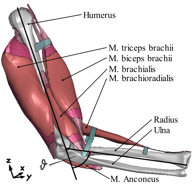
Figure 1: Finite-element model. Rendering of the finite-element upper-limb model, with the definition of the joint angle $\vartheta$. The colours help differentiate between pure muscle (brown-red), a muscle-tendon-mix (magenta), pure tendon (light red) and bands mimicing connective tissue (light blue).

The geometrical (FE) model of the upper limb contains three bones and five muscles (see Figure 1). The bones are modelled as rigid bodies and are namely the humerus, radius, and ulna. Radius and ulna revolve around a hinge joint, connecting them to the lower head of the humerus. The muscles actuating the joint are the m. biceps brachii (biceps), m. brachialis (brachialis), and m. brachioradialis (brachioradialis) for flexion as well as the m. triceps brachii (triceps) and m. anconeus (anconeus) for extension. The distal end of the humerus is fixed and aligned with the z-axis. The anatomical model of our upper limb (Figure 1) is based on the Visible Human dataset [26] and discretised using the FE method. The meshing was done with the pre-postprocessor ANSA. Special attention was given to ensuring sufficient accuracy of element density and element quality. The entire muscle-tendon-system consists of 638 373 tetrahedral, quadratic Lagrange FE elements with 10 nodes each. The biceps by itself, which is in special consideration in this paper, is discretised with 68 292 elements. For the mutual interaction between muscles and muscle with bone, a mortar surface-to-surface contact formulation is applied. The proximal tendons are fixed to the ulna and radius with tied node-to-surface contact formulation.

The constitutive material description used within this work for the second Piola-Kirchhoff stress tensor $\mathbf{S}$ is based on a formulation using the right Cauchy Green tensor that is equivalent to the transversely isotropic muscle-tendon-description proposed by Röhrle et al. [27]. To describe the mechanical behaviour of the skeletal muscles constitutive behaviour, they use a phenomenological approach that is based on the principal invariants $I_{1}=\rm tr[\mathbf{C}]$, $I_{2}=\rm tr[cof[\mathbf{C}]]$, $I_{3}=\det[\mathbf{C}]$ and the current (muscle) fibre stretch $\lambda_{f}=\sqrt{\mathbf{a}\cdot\mathbf{a}}=\sqrt{\rm tr[\mathbf{MC}]}$ with the structure tensor $\mathbf{M}=\mathbf{a}_{0}\otimes\mathbf{a}_{0}$, the referential fibre direction unit vector $\mathbf{a}_{0}$ and “$\otimes$” denoting the dyadic product. The vector $\mathbf{a}_{0}$ relates to its current counterpart via $\mathbf{a}=\mathbf{F}\,\mathbf{a}_{0}$. The stress $\mathbf{S}$ is additively split into an isotropic and an anisotropic term, i.e., $\mathbf{S}=\mathbf{S}_{iso}+\mathbf{S}_{aniso}$, and the anisotropic part is further split to take into account passive anisotropic tissue, e.g., tendon, and active contributions of skeletal muscle tissue, (cf. Klotz et al. [28]):

$$\mathbf{S}=\mathbf{S}_{iso}+(\mathbf{S}_{passive}+\alpha\gamma_{M}\mathbf{S}_{active})(1-\gamma_{ST}),$$ (2)

where $\alpha\in[0,1]$ is the muscle activation, $\gamma_{M},\gamma_{ST}\in[0,1]$ are factors to adjust the tissue compositions, e.g. muscle with $\gamma_{M},\gamma_{ST}>0$), tendon ($\gamma_{M}=0,0<\gamma_{ST}\leq 1$), and fat ($\gamma_{M}=\gamma_{ST}=0$). The isotropic part constitutes a Mooney-Rivlin-type material [29, 30]:

$$\mathbf{S}_{iso}=(B_{1}\mathbf{I}+B_{2}\mathbf{C}+B_{3}\mathbf{C}^{-1})+k\,(I_{3}^{1/2}-1)\,I_{3}^{1/2}\,\mathbf{C}^{-1},$$ (3)

where $k$ is the so-called bulk modulus [31],

$$B_{1} =2c_{1}I_{3}^{-1/3}+2c_{2}I_{3}^{-2/3}I_{1},$$ (4)

$$B_{2} =-2c_{2}I_{3}^{-2/3},\ \text{and}$$ (5)

$$B_{3} =-2/3c_{1}I_{3}^{-1/3}I_{1}-4/3c_{2}I_{3}^{-2/3}I_{2}.$$ (6)

with material parameters $c_{1}$ and $c_{2}$. As described in [27], the passive term $\mathbf{S}_{passive}$ of the anisotropic stress is chosen to be:

$$\mathbf{S}_{passive}=\ \begin{cases}\ \frac{c_{3}}{\lambda_{f}^{2}}\left(\lambda_{f}^{c_{4}}-1\right)\mathbf{M}&\text{for}\ \lambda_{f}\geq 1\ ,\\ \ \mathbf{0}&\text{else}\ ,\end{cases}$$ (7)

where $c_{3}$ and $c_{4}$ are material parameters associated with the anisotropy of the material. The active part $\mathbf{S}_{aniso}$, is given by:

$$\mathbf{S}_{active}=\begin{cases}\frac{S_{max}}{\lambda_{f}^{2}}\exp{\left(-\left|\frac{\lambda_{f}/\lambda_{f}^{opt}-1}{\Delta W_{asc}}\right|^{\nu_{asc}}\right)}\,\mathbf{M}&\text{for}\ \lambda_{f}\leq\lambda_{f}^{opt}\\ \frac{S_{max}}{\lambda_{f}^{2}}\exp{\left(-\left|\frac{\lambda_{f}/\lambda_{f}^{opt}-1}{\Delta W_{desc}}\right|^{\nu_{desc}}\right)}\,\mathbf{M}&\text{for}\ \lambda_{f}>\lambda_{f}^{opt}\ ,\end{cases}$$ (8)

where $S_{max}$ is the maximum active stress a muscle can generate at its optimal fibre length $\lambda_{f}^{opt}$. Furthermore $W_{asc}$ and $\nu_{asc}$ define the ascending part of the force-length-relation of the muscle, while $W_{desc}$ and $\nu_{desc}$ are the corresponding counterparts for the descending part. The material parameters are summarised in Table 1 in the Appendix.

The constitutive material model defined in Eqs (2)-(8) has been implemented as a user-material in the commercial FE software LS-DYNA. An implicit solver is used to solve the appropriate weak form of the linear momentum balance (the governing equation)

$$\textsf{div}\,\mathbf{\sigma}+\rho\,\mathbf{g}=\rho\,\mathbf{\ddot{x}},$$ (9)

in spatial configuration. The stress tensor $\mathbf{S}$ from Eq. (2) is connected to the Cauchy stress tensor in Eq. (9) via $\mathbf{\sigma}=\det[\mathbf{F}]^{-1}\ \mathbf{F}\,\mathbf{S}\,\mathbf{F}^{T}$. Further, $\rho$ is the material density in the current configuration and $\mathbf{g}$ denotes acceleration due to gravity. We expect sufficiently slow movements, $\mathbf{\ddot{x}}\approx\mathbf{0}$, so that the problem becomes quasi-static. To ensure nearly incompressible deformations, $k$ is chosen sufficiently large.
The continuum-mechanical model described in this section constitutes a function $\boldsymbol{\alpha}\rightarrow\mathbf{x}(\mathcal{P}),\ \forall\ \mathcal{P}\in\mathcal{B}$ and $\forall\ \alpha_{i}\in[0,1],\ i=1,..,5$, where $\alpha_{i}$ refers to the activation levels of the individual muscles in the model, while $\boldsymbol{\alpha}$ is a vector containing all five activation values. For the subsequent surrogate modelling we will - without loss of generality - focus on the biceps surface specifically.

2.2 Sparse grid surrogate

With respect to the elbow joint angle the upper limb model represents an overdetermined system. Consequently an optimisation is needed to solve the inverse problem of finding the muscle activation levels necessary to reach a given pose. The original FE model cannot be used to handle this process in a reasonable time span, not even on high-performance hardware. Tests on a cluster with 64 CPUs, with 3 GHz each, and 1 TB of RAM showed evaluation times of up to 4 minutes per deformation state. Instead, FE model evaluations were restricted to 1053 states, uniformly distributed across the 5D parameter space of all activation levels. The number of states and their distribution was chosen to fit the support for a uniform SG. We use this surrogate to interpolate the known activation states, in order to evaluate the displacement for any activation $\alpha_{i}\in[0,1]$. The SG only interpolates in the activation-domain not in space. Strictly speaking we use an ensemble of SGs, one per node in the FE mesh. For the purposes of this paper, we simply refer to this ensemble as a whole as the SG surrogate, which constitutes a function $\alpha\rightarrow\mathbf{x}(P_{mesh}),\ \forall\ P_{mesh}\in\partial\mathcal{B}_{biceps}$, where $P_{mesh}$ refers to mesh node, rather than material points $\mathcal{P}$. The size of the support of a SG is characterised by its level $l$. A higher level results in a more fine-grained grid, allowing for more accurate interpolation. Choosing a level is thus a trade-off between computational cost and accuracy. Based on the previous findings by Valentin et al. a regular SG of level $l=2$ was deemed dense enough to achieve sufficient approximation accuracy. Each activation level of one of the five muscles in the model constitutes one dimension of the SG. Spanning this parameter space with a SG of level 2 requires the aforementioned 1053 unique activation combinations. The interpolation between the support points is based on cardinal B-splines of degree $p=3$. A B-spline $b^{p}:\mathbb{R}\to\mathbb{R}$ is defined recursively by:

$$b^{0}(x)=1_{[0,1)}(x),\ \ b^{p}(x)=\int_{0}^{1}b^{p-1}(x-y)dy\ \ .$$ (10)

The hierarchisation of these splines is given as the affine transformation

$$\varphi^{p}_{l,i}(x)=b^{p}\left(\frac{x}{h_{l}}+\frac{p+1}{2}-i\right),\ \ h_{l}=2^{-l}\ \ .$$ (11)

For SGs of dimension $d$, multivariate, hierarchical B-splines are obtained by computing a tensor product

$$\varphi^{\mathbf{p}}_{\mathbf{l},\mathbf{i}}(\mathbf{x})=\prod^{d}_{t=1}\varphi^{p_{t}}_{l_{t},i_{t}}(x_{t}),\ \ \mathbf{l}\in\mathbb{N}^{d},\ \mathbf{i}\in I_{\mathbf{l}}=I_{l_{1}}\times,...,\times I_{l_{d}}\ \ ,$$ (12)

with corresponding grid-points

$$\mathbf{x}_{\mathbf{l},\mathbf{i}}=(x_{l_{t},i_{t}})_{t=1,..,d},\ \ x_{l_{t},i_{t}}=i_{t}\cdot h_{l_{t}}\ \ .$$ (13)

In the multivariate case $\mathbf{i}$ and $\mathbf{l}$ encompass all indices and levels associated with a given quantity, as both of those are defined per input dimension and can vary between them. Valentin and Pflüger showed that for odd $p$ the nodal subspace $V_{l}^{p}$ of a regular SG of level $l$ and dimension $d$ can be described by the direct sum:

$$V_{\mathbf{l}}^{\mathbf{p}}=\underset{\parallel\mathbf{l}\parallel_{1}\leq n+d-1}{\oplus}\text{span}\{\varphi^{\mathbf{p}}_{\mathbf{l},\mathbf{i}}|\mathbf{i}\in I_{\mathbf{l}}\}$$ (14)

The contribution of each subspace to the approximation $\hat{f}$ of a given function $f:[0,1]\to\mathbb{R}$ is controlled by weighting-coefficients, the so-called hierarchical surpluses $\alpha_{l^{\prime},i^{\prime}}$, and defined by

$$\hat{f}(\mathbf{x})=\sum_{l^{\prime}=0}^{l}\sum_{i^{\prime}\in I_{l^{\prime}}}\alpha_{l^{\prime},i^{\prime}}\varphi_{l^{\prime},i^{\prime}}(\mathbf{x})\ ,$$ (15)

with

$$\hat{f}(x_{l,i})=f(x_{l,i})\ \ \forall i\in\left[0,2^{l}\right]\ .$$ (16)

2.3 Neural network surrogate

With sparse-grid-surrogate evaluation times of up to 100 ms for the visualisation of the biceps’ surface, the SG surrogate is significantly faster than the original FE simulation but not fast enough for real-time visualisation. Thus results from SG interpolation are used as training data for a real-time-capable deep learning surrogate. To predict the activation- and stretch-induced deformation of the biceps’ surface in real-time, a densely connected feed-forward neural network (NN) is employed. Note, the NN surrogate is not supposed to be a one-to-one replacement for the SG. As the relation between joint angle and muscle activation input might not be bijective, i.e.  multiple joint angles might relate to the same muscle activation levels, we additionally desire "energy efficiency of the musculoskeletal system", i.e. penalising sets of activation levels with high values.

Within this work, we achieve this by defining the following cost function for the optimisation:

$$\boldsymbol{\alpha}^{\mbox{k}}_{\mbox{opt}}=\underset{\boldsymbol{\alpha}^{\mbox{k}}\in[0,1]^{5}}{\text{argmin}}\,\left(\left|{\varTheta^{\mbox{k}}}-\vartheta^{\mbox{k}}(\boldsymbol{\alpha}^{\mbox{k}})\right|+0.05\cdot\sum_{i=1}^{5}\alpha^{\mbox{k}}_{i}\right)\ \ ,$$ (17)

where $\varTheta^{\mbox{k}}$ is the target elbow angle and $\vartheta(\boldsymbol{\alpha}^{\mbox{k}})$ is the in silico determined elbow angle due to activation parameters $\boldsymbol{\alpha}^{\mbox{k}}$. The scaling of the sum of the activation levels has been chosen small, i.e. $0.05$, keeping the focus of the minimisation on target angle $\varTheta^{\mbox{k}}$.

To speed up the activation-joint-angle-relationship calculations during the online phase, we evaluate equation (17) for a set of admissible activation parameters ($$10\text{\,}\mathrm{\SIUnitSymbolDegree}$\leq\varTheta^{\mbox{k}}\leq$150\text{\,}\mathrm{\SIUnitSymbolDegree}$$) and subsequently use the $\boldsymbol{\alpha}^{\mbox{k}}_{\mbox{opt}}$ within a SG surrogate for the deformation of each mesh node on the muscles’ surface. As we consider quasi-static conditions, we omit superscript $k$ for the time instance from now on. The deformation is then used to train a NN surrogate, i.e. it is trained to approximate a function $\boldsymbol{\alpha}_{\text{opt}}\rightarrow\mathbf{u}(P_{mesh}),\forall\ P_{mesh}\in\partial\mathcal{B}_{biceps}$. This is obtained by evaluating the SG surrogate for all the mesh-nodes $P_{mesh}$ at $\boldsymbol{\alpha}_{\mbox{opt}}$, and subtracting the known reference coordinates of the given node $\mathbf{X}(P_{mesh})$ from the result. All these evaluations and the training of the network can be done during the offline phase. The reference configuration is added to the bias of the last layer in the NN post-training, to convert from the displacement back to the Cartesian coordinates of the mesh-nodes. With this the NN surrogate provides the desired function $\boldsymbol{\alpha}_{\text{opt}}\rightarrow\mathbf{x}(P_{mesh}),\forall\ P_{mesh}\in\partial\mathcal{B}_{biceps}$.

The NN was implemented using the open-source API Keras for TensorFlow in Python [33, 34].

2.3.1 Neural Network Architecture

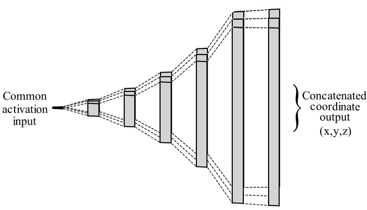
Figure 2: Combined model. Combination of the three NNs for the x-, y- and z-coordinate, by defining a common input for all three networks and a concatenated output.

The NN architecture needs to bridge the gap between the number of inputs $n_{in}=5$, i.e. the number of muscle activation parameters of the FE model, and the number of outputs $n_{out}=2809$. The NN consists entirely of densely connected layers. While there are three Cartesian coordinates to consider for each node, the coordinate directions are trained separately, each using an identical architecture. The reasons for this will be discussed in more detail in the next section. The width $w$ of each layer, i.e. the number of neurons per layer, increases exponentially from input to output of the NN. The parameters of the exponential function are the number of hidden layers $n_{hidden}$, $n_{inputs}$, $n_{outputs}$, and $n_{mid}$, which specifies the width to be reached half-way between the input- and output-layer:

$$w(n) =a\cdot e^{b\cdot n}+c\ ,\ \text{with}$$ (18)

$$a =\frac{n_{mid}^{2}-n_{inputs}^{2}}{n_{outputs}-2\cdot n_{mid}-n_{inputs}}\ ,$$ (19)

$$b =2\cdot n_{hidden}\cdot\log(\frac{n_{outputs}+n_{inputs}}{n_{mid}+n_{inputs}})\ ,$$ (20)

$$c =n_{inputs}-a\ \ .$$ (21)

Figure 2 shows a visual representation of this NN architecture. The best training results were reached with the number of hidden layers $n_{hidden}=5$ and the width of the mid-layer of the network $n_{mid}=700$. These parameters were chosen as small as possible, while maintaining sufficient accuracy, i.e. sufficiently low mean squared error (MSE), of the predicted coordinate output, by comparing NNs with varying values for these parameters.

2.3.2 Dimension-decoupled training

Three individual networks were trained, one for each coordinate dimension. Post-training, these individual models were combined into a single NN via network-graph redefinition, using the Keras functional API 2). Each of the three networks was trained using five-fold cross-validation [35], i.e. the training data was shuffled, and divided into five partitions, one of which was used for validation and four for training for a certain number of epochs defined. After each “fold”, which partition is used for validation and thus not shown to the model during training changes. The networks were trained for 400 epochs on each fold, resulting in an overall training duration of 2000 epochs on the MSE, with the mean absolute error (MAE) as an additional metric. Here “mean” refers to a mean value across all surface nodes in a given configuration. Additionally Keras’ “callbacks”-functionality was used to select the version of the NN that performed best, i.e. has the lowest loss across all epochs. This was done to account for fluctuations in the in-training performance from epoch to epoch, meaning the last iteration of the NN was not necessarily the best performing one. Keras’ functional API allows for the redefinition of network-graphs on a layer-by-layer basis. This was used to define a common input and output for the three networks, without needing to manipulate their tensors manually. The only manual weight-editing is the aforementioned addition of the reference configuration to the last layer’s bias, converting the NN’s output from displacement to Cartesian coordinates.

3 Results

3.1 Performance results

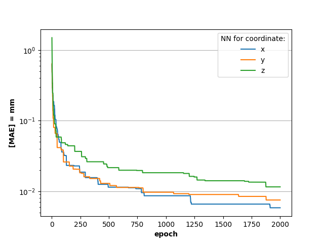
Figure 3: Training history. In-training performance of the three coordinate-networks shown as the MAE in mm over the number of epochs trained.

Figure 3 shows the performance of the current lowest loss model over the course of 2000 epochs of training. For reference, without the use of callbacks the model loss fluctuated between $1\cdot 10^{-1}$ and $1\cdot 10^{-2}$ mm of MAE. The initial drop in loss over the first 50 epochs was not subject to these fluctuations.

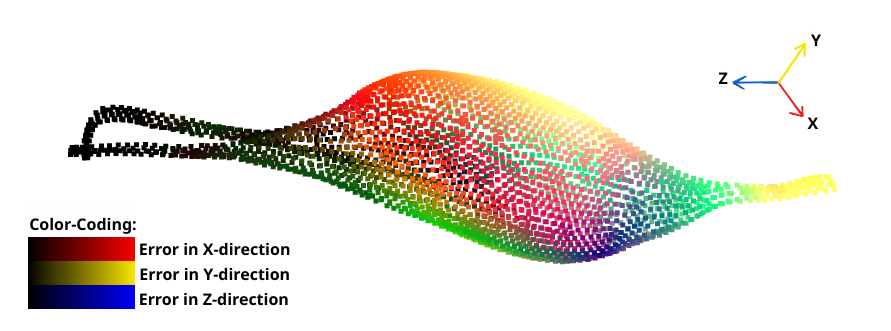
Figure 4: Error “hot-spots”. Qualitative error analysis after 100 epochs of training, with colour-coding for x (red), y (yellow), z (blue). Yellow regions of comparatively high error appear in multiple configurations.

In the intermediate results from the first 100 epochs of training the accuracy of the predicted node coordinates differed significantly across the biceps’ surface. More specifically, while visualising a cycle of arm flexion and extension, consistent areas of high absolute error. This did not correspond to a higher MAE than for other surface configurations. This mostly concerned configurations for which all flexors were at least partially activated. An example of a configuration exhibiting these hot-spots can be seen in Figure 4, where the higher the MAE, the lighter the colour of the area. These regions, in order of decreasing MAE, are namely the lower tendon, the medial side of the biceps’ belly, as well as the more lateral, dorsal area of the muscle belly. The error distribution across the muscle equalised over the rest of training and hot-spots were no longer present by the end of it. In-training accuracy after 2000 epochs showed a maximum absolute error (MaxAE) of 0.37 mm, which corresponds to 0.38%, with a mean error of 0.014 mm. All three of these values give an average over all evaluated states, with mean and maximum taken for each.
Out-of-training performance was tested by iteratively generating random activation vectors for which both the NN and the SG were evaluated. Out-of-training performance refers to a NN generalisation capabilities, i.e. generating output for inputs that were not included in the training data. This still holds true in our case, but does not include any extrapolation, since our input parameter space is strictly bounded. New random activation vectors were tested until the highest recorded MaxAE of the NN w.r.t. the SG no longer increased for 300 consecutive iterations, i.e. until a worst-case accuracy was found. The results were a maximum MaxAE of 8.82 mm and maximum relative error (MaxRE) of 10.12%. Here, the MaxRE is not the converted MaxAE, but rather a separately recorded maximum value. The highest MAE across all configurations was 1.69 mm, the highest mean relative error (MRE) 1.23%.
Random sampling will include activation vectors, which will not be encountered in the final application, as they are not an optimal choice for any given joint angle. Instead iteratively testing for random joint angles, for which the optimal activations are computed, yields a MaxAE of 3.75 mm and a MaxRE of 5.69%, a MAE of 0.97 mm and a MRE of 0.57%. See Table 1 for a summary of these results.

Table 1: Out-of-training accuracy. Summary of the out-of-training accuracy of the NN tested on random activations and optimal activations for random joint angles. Relative erros were determined independently from the absolute values.

	maximum error		mean error
tested for:	mm	%	mm	%
random	11.96	13.28	2.15	1.59
activation
random	3.75	5.69	0.97	0.57
angle

The model was also tested for evaluation speed. This was done for sequential execution of the three separate NNs for the x-, y- and z-coordinate, the combined model as shown in Figure 2, and a TensorFlow-Lite-version of the combined model. The models were tested on CPU only (Intel i5 with 6 cores with 3 GHz) and with GPU support (Nvidia Geforce GTX 1650 with 4GB VRAM).

Table 2: Average evaluation times. Comparison of evaluation times of different versions of the NN model, averaged over 1000 evaluations.

Model version	Evaluation time in ms
three separate models	13.65
$\to$ with GPU	4.05
combined model	13.34
$\to$ with GPU	3.48
combined model Lite	9.88

Table 2 shows the evaluation times averaged over 1000 evaluations are approximately the same for the sequential and the combined model when executed on the CPU, with a theoretical frame rate of about 75 frames per second (fps). For execution on the GPU the times differs, with the combined model being 0.57 ms faster than the sequentially executed models. The theoretically achievable frame rates are 246.91 fps and 287.36 fps respectively. The results for the TensorFlow Lite model are identical for GPU and CPU, with an evaluation time of 9.88 ms, i.e. 101.21 fps.

3.2 Error Propagation

Since the NN surrogates are trained on data from the SG surrogate, not the FE simulation, i.e. approximating based on an approximation, error propagation should be considered. The worst case scenario would be that the NN amplifies the approximation error of the SG. To investigate this the FE model was run for 25 activation combinations drawn randomly from a uniform distribution. Both the SG and the NN surrogate were evaluated for the same activation vectors and the results of the subsequent comparison of both to the FE simulation are summarised in Table 3.

Table 3: Error propagation test. Summary of the accuracy of the SG and the NN tested on 25 random activations evaluated using the FE model. The NN was also tested on the 1053 support-points of the SG, since those are taken from the FE-model as well.

	maximum error		mean error
Surrogate:	mm	%	mm	%
SG	17.79	10.14	2.86	1.52
NN	18.28	9.38	2.84	1.45

The error of the NN with respect to the original FE simulation closely matches that of the SG, both with significant inaccuracies. Put differently, the SG appears to be the primary contributor to the overall approximation error of the surrogate system, while the NN does not notably add to it (see also 1).

4 Discussion

Results derived using short training times revealed error hot-spots, as shown in Figure 4, which were found to be consistent in most surface configurations. These regions of comparatively high error on the biceps’ belly coincide with contact areas with other flexors, like the M. brachioradialis (BR). A possible explanation for the apparent increased learning complexity in these regions is contact to the BR deflecting surface nodes from a more common trajectory. Trajectories of nodes in these regions are likely more unique compared to the majority of nodes. Deflection of the biceps by the BR is likely aggravated by the lack of a fat-skin-layer surrounding the musculature, causing the BR to contract less in line with the humerus and biceps, than it realistically would. Implementation of a fat-skin-layer is already planned for future versions of this model. The tip of the lower tendon of the biceps is also an area of comparatively high error, which is caused by its attachment to the radius bone. Movement of these nodes is determined by the rotation of the lower arm around the elbow joint, which again results in node trajectories unlike the majority throughout the muscle. Deep learning models, especially classifiers, which sort data into categories, are known to have difficulties learning rare cases in their training data. Data augmentation techniques can be used to make rare occurrences more prevalent in the data, increasing their influence during training [36]. A similar effect could be achieved for our regression model, e.g. by subdividing the NN model into parts specialising in these regions and nodes. However, since the hot-spots vanish given sufficient training time, data augementation will not be necessary in this case. It is interesting to see muscle-to-muscle contact have this effect nonetheless.

4.1 Out-of-Training Performance

Out-of-training accuracy was within expectations. While the NN can not provide the level of accuracy of the original simulation or the in-training accuracy, even the worst case accuracy shown in Table 1, with 5.69% MaxRE and 3.75 mm MaxAE, are not of concern for visualisation-purposes. Especially considering the MAE and MRE are an order of magnitude below the worst case performance, with 0.97 mm and 0.57%. The final application envisioned by this project will include additional, external computational resources, as well as a number of models with different complexity and accuracy. Which model to use, and how heavily computations are offloaded, will be decided by the application at run-time, to provide the best possible performance depending on the available hardware. The additional results regarding error propagation shown in Table 3 show inaccuracies of the SG to dominate the overall error. These inaccuracies can not be disregarded as fringe effects, as they occur at mid level activations. The current SG is uniform in all five activation dimensions. This can be improved upon by building the SG support adaptively, which involves evaluating SG accuracy while building its support by running the FE-model, iteratively adding support points as and where needed [37]. Which points are most likely to improve accuracy the most can be estimated, as for example demonstrated by Khakhutskyy and Hegland. An adaptive SG will be implemented in next version of this setup.
There is an overarching point to be made about error propagation with coupled surrogate models, as we use them here. Deep learning models are black-boxes with no formal way for predicting their accuracy, and are highly dependent on the quality of their training data [39]. Continuum mechanics relies on homogenisation of the micro-scale, while the FE method introduces a discretisation error. Care needs to be taken, when chaining models and methods in this manner, with a data driven model as the endpoint. This is however mitigated by the fact that the strength and weaknesses of both the FE method, continuum mechanics, and SG are well and formally established [40, 41].
The measured evaluation times (see Table 2) shows that all tested versions of the model are real-time-capable. A conversion to an optimised format, such as TensorFlow Lite, is preferable, if no GPU is available. TensorFlow Lite is optimised for ARM CPUs, to better fit mobile devices, where they are commonly used. Thus, the results listed here, likely do not show the peak performance of the TensorFlow Lite version of the model, since the Intel CPU we tested on is of a different architecture.
It is already known from preliminary tests that running the NN model will not be the biggest contributor to the overall computational load of the target application. This will rather be the motion tracking needed to estimate the pose of a person the model is supposed to be overlayed on in VR/AR, as well as the visualisation of the model. Fortunately all versions of the model tested here lie well below the guideline for real-time applications of 30 ms evaluation time, leaving us with computational resources to spare at the current accuracy and speed.

4.2 Architecture Design process

Since a significant part of the results of this work is the specialised NN-architecture, we would like to give some insight into its construction.
Fully connected layers were used for this model, as there was nothing about the data indicating an immediate benefit from using a more specialised layer-type. It also offered the most flexibility in shaping the architecture overall. To connect the five input parameters to the 2809 outputs, three rudimentary options came to mind:

1. changing the layer-width as late as possible, resulting in a T-shaped NN

2. changing the layer-width as early as possible, resulting in a rectangular NN

3. changing the layer-width linearly as a function of the distance to the input, resulting in a triangular NN

To be able to compare these three architectures, prototypes were generated with an arbitrarily chosen 10 hidden layers.

Table 4: Prototyping. Comparison of three different prototype-architectures for learning the X-coordinates of the biceps’ mesh, based on in-training MAE after 10 epochs, and number of trainable parameters.

	T-shaped	rectangular	triangular
# of Parameters	17.154	71.056.494	26.103.046
MAE in mm	430	2.4	2.2

As this was only the initial prototyping stage, short training times of only 10 epochs were deemed sufficient to check if a particular network shape would lend itself to the data. An example of such a test can be seen in Table 4. In this comparison the T-shaped architecture performs significantly worse than its competitors. The rectangular and triangular architectures are on par. However the triangular architecture reaches this level of accuracy with less than half the number of trainable parameters of the rectangular one. The exponential architecture introduced in the Methods section was then developed in an attempt to further decrease the number oftrainable parameters, by slimming its mid-section, without loss in accuracy. The number of hidden layer was then iteratively decreased down to five, at which point further reduction caused a notable decline in training accuracy. The same was done for the width of the mid-layer of the model (see 21).
These initial steps were taken while training on the nodal coordinates, not the deformation. However, first visualisations using this method, revealed the biceps to slightly drift sideways during contraction. Switching to training on the deformation instead successfully removed any drift from the predicted nodal positions. Further improvements were then simply achieved with longer training times.
All these steps could be done by considering only one of the three output dimensions. When trying to expand the architecture to 3D, with the same number of hidden layers and shape, training performance was significantly worse. To circumvent this problem, without increasing the size of the NN, three individual networks were trained, one for each coordinate dimension, and combined into a single NN via network-graph redefinition post-training.

5 Conclusion and outlook

The aim of this work was to find a work flow that is suitable for visualising data from continuum-mechanical forward simulations in real-time, to further the development of pervasive simulation and open up continuum mechanics to a wider variety of applications. The presented proof-of-concept model is able to predict the surface configuration of the biceps, based on a vector of activation levels optimal for reaching a certain target elbow angle, within an average error of 0.97 mm at a frame rate of up to 287.35 fps on non-high-end hardware. This model thus fulfills our set criteria. Also note that even taking the aim of pervasiveness aside, real-time prediction of the muscle’s surface configuration on a non-high-end PC, is still an exciting result, considering the original FE simulation took minutes per configuration on 64 CPUs à 3GHz, with 1 TB of RAM. The use of a SG surrogate to generate the training data for the NN, has proved efficient for acquiring arbitrary amounts of training data within a feasible time frame. Accuracy of the SG still needs to be improved by optimising its support. Next steps are the expansion of this workflow to the full FE model, including five muscles and three bones, contributing to a complete simulation of the upper arm.
These models will be implemented and extensively tested on resource-constraint devices, e.g. a distributed AR application on the Microsoft HoloLens 2. To achieve this, firstly a second model trained on the relationship between the motion tracking data (elbow angle, angular velocity and acceleration) and the optimal activation vectors will be introduced; secondly, once the output visualisation is overlayed onto a person, it will be supplemented with additional biomechanical information, e.g. graphs tracking the activation levels. A scenario these two steps will be relevant for is for example coupling the model to a motion guidance system for physiotherapy or exercise.
For instance, in the physiotherapy setting, a doctor asks their patient to complete an arm movement following a guided path, shown to them in VR/AR. This model could help the patient to appreciate how their motions result from muscle contraction and aid the physiotherapist in explaining possible issues and solutions. Ideally, this could allow the patient to share in their therapist’s intuition as to what needs to be done. The guidance could help provide feedback to the patient on what exactly the motion is, they should try to achieve [42, 43], even continue to do so, when training unsupervised at home [44]. Further development of this model beyond the technical aspects will include incorporating it into new on-body interaction techniques, to not only further improve performance on a wider range of hardware, but also provide ease of use to the end-user.
Finally, we would like to note that the methods presented in this paper are neither limited to the muscle constitutive laws chosen in Section 2.1 nor to FE results in general. The presented sparse-grid-neural-network workflow is equally applicable to more complex, microstructural-based muscle constitutive laws [45] or activation mechanisms [28], as well as to other biological or man-made materials. Likewise, the method can be applied to any kind of mesh-based data, such as results coming from the finite-difference-method.

Appendix A Constitutive parameters

Table 1: Model parameters. Constitutive parameters for the muscle-tendon-complex of the biceps.

Parameter	Value	Source
$c^{M}_{1}$	$3.56\cdot 10^{-2}$ MPa	Hawkins and Bey [46]
$c^{M}_{2}$	$3.86\cdot 10^{-3}$ MPa
$c^{M}_{3}$	$3.57\cdot 10^{-8}$ MPa	Zheng et al. [47]
$c^{M}_{4}$	42.6
$c^{T}_{1}$	2.31 MPa	Weiss and Gardiner [48]
$c^{T}_{2}$	$1.15\cdot 10^{-6}$ MPa
$c^{T}_{3}$	7.99 MPa
$c^{T}_{4}$	16.6
$\Delta W_{asc}$	0.25	adapted from Günther et al. [49]
$\Delta W_{desc}$	0.15
$\nu_{asc}$	3.00
$\nu_{desc}$	4.00
$\lambda_{o}pt^{f}$	1.35
$\sigma_{max}$	0.30 MPa

Data availability

Sparse grid data, training data, and code for the models presented here will be made available on https://darus.uni-stuttgart.de upon peer-reviewed publication of this manuscript.

References

- Sadeghi et al. [2020] Amir H Sadeghi, Sulayman El Mathari, Djamila Abjigitova, Alexander PWM Maat, Yannick JHJ Taverne, Ad JJC Bogers, and Edris AF Mahtab. Current and future applications of virtual, augmented, and mixed reality in cardiothoracic surgery. The Annals of Thoracic Surgery, 2020.
- Allard et al. [2007] Jérémie Allard, Stéphane Cotin, François Faure, Pierre-Jean Bensoussan, François Poyer, Christian Duriez, Hervé Delingette, and Laurent Grisoni. Sofa-an open source framework for medical simulation. In MMVR 15-Medicine Meets Virtual Reality, volume 125, pages 13–18. IOP Press, 2007.
- Ghannadi et al. [2017] Borna Ghannadi, Naser Mehrabi, Reza Sharif Razavian, and John McPhee. Nonlinear model predictive control of an upper extremity rehabilitation robot using a two-dimensional human-robot interaction model. In 2017 IEEE/RSJ International Conference on Intelligent Robots and Systems (IROS), pages 502–507. IEEE, 2017.
- Hill [1938] Archibald Vivian Hill. The heat of shortening and the dynamic constants of muscle. Proceedings of the Royal Society of London. Series B-Biological Sciences, 126(843):136–195, 1938.
- Zajac [1989] Felix E Zajac. Muscle and tendon: properties, models, scaling, and application to biomechanics and motor control. Critical reviews in biomedical engineering, 17(4):359–411, 1989.
- Meszaros-Beller et al. [2023] Laura Meszaros-Beller, Maria Hammer, Syn Schmitt, and Peter Pivonka. Effect of neglecting passive spinal structures: a quantitative investigation using the forward-dynamics and inverse-dynamics musculoskeletal approach. Frontiers in Physiology, 14:1135531, 2023.
- Van den Bogert et al. [2013] Antonie J Van den Bogert, Thomas Geijtenbeek, Oshri Even-Zohar, Frans Steenbrink, and Elizabeth C Hardin. A real-time system for biomechanical analysis of human movement and muscle function. Medical & biological engineering & computing, 51(10):1069–1077, 2013.
- Ezati et al. [2019] Mahdokht Ezati, Borna Ghannadi, and John McPhee. A review of simulation methods for human movement dynamics with emphasis on gait. Multibody System Dynamics, 47(3):265–292, 2019.
- Böl et al. [2019] Markus Böl, Rahul Iyer, Johannes Dittmann, Mayra Garcés-Schröder, and Andreas Dietzel. Investigating the passive mechanical behaviour of skeletal muscle fibres: Micromechanical experiments and bayesian hierarchical modelling. Acta Biomaterialia, 92:277–289, 2019.
- Klotz et al. [2020] Thomas Klotz, Leonardo Gizzi, Utku Ş Yavuz, and Oliver Röhrle. Modelling the electrical activity of skeletal muscle tissue using a multi-domain approach. Biomechanics and modeling in mechanobiology, 19(1):335–349, 2020.
- Bradley et al. [2018] Chris P. Bradley, Nehzat Emamy, Thomas Ertl, Dominik Göddeke, Andreas Hessenthaler, Thomas Klotz, Aaron Krämer, Michael Krone, Benjamin Maier, Miriam Mehl, Tobias Rau, and Oliver Röhrle. Enabling detailed, biophysics-based skeletal muscle models on hpc systems. Frontiers in physiology, 9:816, 2018.
- Maier et al. [2019] B Maier, N Emamy, A Krämer, and M Mehl. Highly parallel multi-physics simulation of muscular activation and emg. In COUPLED VIII: proceedings of the VIII International Conference on Computational Methods for Coupled Problems in Science and Engineering, pages 610–621. CIMNE, 2019.
- Maier et al. [2021] Benjamin Maier, Dominik Göddeke, Felix Huber, Thomas Klotz, Oliver Röhrle, and Miriam Schulte. Opendihu—efficient and scalable software for biophysical simulations of the neuromuscular system. Submitted to Journal of Computational Physics, September 2021. 3.553.
- Röhrle [2018] Oliver Röhrle. Skeletal muscle modelling. Encyclopaedia for Continuum Mechanics Section Biomechanics, 2018.
- de Borst [2018] René de Borst. Finite Element Methods. Springer Berlin Heidelberg, Berlin, Heidelberg, 2018. ISBN 978-3-662-53605-6. doi: 10.1007/978-3-662-53605-6_13-1. URL https://doi.org/10.1007/978-3-662-53605-6_13-1.
- Bro-Nielsen and Cotin [1996] Morten Bro-Nielsen and Stephane Cotin. Real-time volumetric deformable models for surgery simulation using finite elements and condensation. In Computer graphics forum, volume 15-3, pages 57–66. Wiley Online Library, 1996.
- Mendizabal et al. [2020] Andrea Mendizabal, Pablo Márquez-Neila, and Stéphane Cotin. Simulation of hyperelastic materials in real-time using deep learning. Medical image analysis, 59:101569, 2020.
- Lloyd et al. [2012] John E Lloyd, Ian Stavness, and Sidney Fels. Artisynth: A fast interactive biomechanical modeling toolkit combining multibody and finite element simulation. Soft tissue biomechanical modeling for computer assisted surgery, pages 355–394, 2012.
- Angles et al. [2019] Baptiste Angles, Daniel Rebain, Miles Macklin, Brian Wyvill, Loic Barthe, JP Lewis, Javier Von Der Pahlen, Shahram Izadi, Julien Valentin, Sofien Bouaziz, et al. Viper: Volume invariant position-based elastic rods. Proceedings of the ACM on Computer Graphics and Interactive Techniques, 2(2):1–26, 2019.
- Taç et al. [2023] Vahidullah Taç, Kevin Linka, Francisco Sahli-Costabal, Ellen Kuhl, and Adrian Buganza Tepole. Benchmarking physics-informed frameworks for data-driven hyperelasticity. Computational Mechanics, pages 1–17, 2023.
- Platzer et al. [2021] Auriane Platzer, Adrien Leygue, Laurent Stainier, and Michael Ortiz. Finite element solver for data-driven finite strain elasticity. Computer Methods in Applied Mechanics and Engineering, 379:113756, 2021.
- Eggersmann et al. [2019] Robert Eggersmann, Trenton Kirchdoerfer, Stefanie Reese, Laurent Stainier, and Michael Ortiz. Model-free data-driven inelasticity. Computer Methods in Applied Mechanics and Engineering, 350:81–99, 2019.
- Holzapfel et al. [2021] Gerhard A Holzapfel, Kevin Linka, Selda Sherifova, and Christian J Cyron. Predictive constitutive modelling of arteries by deep learning. Journal of the Royal Society Interface, 18(182):20210411, 2021.
- Valentin et al. [2018] J Valentin, M Sprenger, D Pflüger, and O Röhrle. Gradient-based optimization with b-splines on sparse grids for solving forward-dynamics simulations of three-dimensional, continuum-mechanical musculoskeletal system models. International journal for numerical methods in biomedical engineering, 34(5):e2965, 2018.
- Kneifl et al. [2023] Jonas Kneifl, David Rosin, Okan Avci, Oliver Röhrle, and Jörg Fehr. Low-dimensional data-based surrogate model of a continuum-mechanical musculoskeletal system based on non-intrusive model order reduction. Archive of Applied Mechanics, 93(9):3637–3663, 2023.
- Ackerman [1998] Michael J Ackerman. The visible human project. Proceedings of the IEEE, 86(3):504–511, 1998.
- Röhrle et al. [2017] O Röhrle, M Sprenger, and S Schmitt. A two-muscle, continuum-mechanical forward simulation of the upper limb. Biomechanics and modeling in mechanobiology, 16(3):743–762, 2017.
- Klotz et al. [2021] Thomas Klotz, Christian Bleiler, and Oliver Röhrle. A physiology-guided classification of active-stress and active-strain approaches for continuum-mechanical modeling of skeletal muscle tissue. Frontiers in Physiology, 12, 2021.
- Mooney [1940] Melvin Mooney. A theory of large elastic deformation. Journal of applied physics, 11(9):582–592, 1940.
- Rivlin [1948] Ronald S Rivlin. Large elastic deformations of isotropic materials iv. further developments of the general theory. Philosophical transactions of the royal society of London. Series A, Mathematical and physical sciences, 241(835):379–397, 1948.
- Crisfield [1991] Michael A Crisfield. Nonlinear finite element analysis of solids and structures. Volume 1: Essentials. Wiley, New York, NY (United States), 1991.
- Valentin and Pflüger [2016] Julian Valentin and Dirk Pflüger. Hierarchical gradient-based optimization with b-splines on sparse grids. In Sparse Grids and Applications-Stuttgart 2014, pages 315–336. Springer, 2016.
- Abadi et al. [2015] Martín Abadi, Ashish Agarwal, Paul Barham, Eugene Brevdo, Zhifeng Chen, Craig Citro, Greg S. Corrado, Andy Davis, Jeffrey Dean, Matthieu Devin, Sanjay Ghemawat, Ian Goodfellow, Andrew Harp, Geoffrey Irving, Michael Isard, Yangqing Jia, Rafal Jozefowicz, Lukasz Kaiser, Manjunath Kudlur, Josh Levenberg, Dandelion Mané, Rajat Monga, Sherry Moore, Derek Murray, Chris Olah, Mike Schuster, Jonathon Shlens, Benoit Steiner, Ilya Sutskever, Kunal Talwar, Paul Tucker, Vincent Vanhoucke, Vijay Vasudevan, Fernanda Viégas, Oriol Vinyals, Pete Warden, Martin Wattenberg, Martin Wicke, Yuan Yu, and Xiaoqiang Zheng. TensorFlow: Large-scale machine learning on heterogeneous systems, 2015. URL https://www.tensorflow.org/. Software available from tensorflow.org.
- Chollet et al. [2015] François Chollet et al. Keras. https://keras.io, 2015.
- Ojala and Garriga [2010] Markus Ojala and Gemma C Garriga. Permutation tests for studying classifier performance. Journal of machine learning research, 11(6), 2010.
- Lim et al. [2018] Swee Kiat Lim, Yi Loo, Ngoc-Trung Tran, Ngai-Man Cheung, Gemma Roig, and Yuval Elovici. Doping: Generative data augmentation for unsupervised anomaly detection with gan. In 2018 IEEE international conference on data mining (ICDM), pages 1122–1127. IEEE, 2018.
- Valentin [2019] Julian Valentin. B-splines for sparse grids: Algorithms and application to higher-dimensional optimization. arXiv preprint arXiv:1910.05379, 2019.
- Khakhutskyy and Hegland [2016] Valeriy Khakhutskyy and Markus Hegland. Spatially-dimension-adaptive sparse grids for online learning. In Sparse Grids and Applications-Stuttgart 2014, pages 133–162. Springer, 2016.
- Miotto et al. [2018] Riccardo Miotto, Fei Wang, Shuang Wang, Xiaoqian Jiang, and Joel T Dudley. Deep learning for healthcare: review, opportunities and challenges. Briefings in bioinformatics, 19(6):1236–1246, 2018.
- Bonet and Wood [1997] Javier Bonet and Richard D Wood. Nonlinear continuum mechanics for finite element analysis. Cambridge university press, 1997.
- Wriggers [2013] Peter Wriggers. Nichtlineare finite-element-methoden. Springer-Verlag, 2013.
- Han et al. [2016] Ping-Hsuan Han, Kuan-Wen Chen, Chen-Hsin Hsieh, Yu-Jie Huang, and Yi-Ping Hung. Ar-arm: Augmented visualization for guiding arm movement in the first-person perspective. In Proceedings of the 7th Augmented Human International Conference 2016, pages 1–4, 2016.
- Yu et al. [2020] Xingyao Yu, Katrin Angerbauer, Peter Mohr, Denis Kalkofen, and Michael Sedlmair. Perspective matters: Design implications for motion guidance in mixed reality. In 2020 IEEE International Symposium on Mixed and Augmented Reality (ISMAR), pages 577–587. IEEE, 2020.
- Tang et al. [2015] Richard Tang, Xing-Dong Yang, Scott Bateman, Joaquim Jorge, and Anthony Tang. Physio@ home: Exploring visual guidance and feedback techniques for physiotherapy exercises. In Proceedings of the 33rd Annual ACM Conference on Human Factors in Computing Systems, pages 4123–4132, 2015.
- Bleiler et al. [2019] Christian Bleiler, Pedro Ponte Castañeda, and Oliver Röhrle. A microstructurally-based, multi-scale, continuum-mechanical model for the passive behaviour of skeletal muscle tissue. Journal of the Mechanical Behavior of Biomedical Materials, 97:171–186, 2019. doi: 10.1016/j.jmbbm.2019.05.012.
- Hawkins and Bey [1994] D Hawkins and M Bey. A comprehensive approach for studying muscle-tendon mechanics. Journal of biomechanical engineering, 116(1):51–55, 1994.
- Zheng et al. [1999] Yong-Ping Zheng, Arthur FT Mak, Bokong Lue, et al. Objective assessment of limb tissue elasticity: development of a manual indentation procedure. Journal of Rehabilitation Research and Development, 36(2):71–85, 1999.
- Weiss and Gardiner [2001] Jeffrey A Weiss and John C Gardiner. Computational modeling of ligament mechanics. Critical Reviews™ in Biomedical Engineering, 29(3), 2001.
- Günther et al. [2007] Michael Günther, Syn Schmitt, and Veit Wank. High-frequency oscillations as a consequence of neglected serial damping in hill-type muscle models. Biological cybernetics, 97(1):63–79, 2007.