Voting models and tightness for a family of recursion equations

Abstract

We consider recursion equations of the form $u_{n+1}(x)=Q[u_{n}](x),\leavevmode\nobreak\ n\geq 1,\leavevmode\nobreak\ x\in{\mathbb{R}}$, with a non-local operator $Q[u](x)=g(u\ast q)$, where $g$ is a polynomial, satisfying $g(0)=0$, $g(1)=1$, $g((0,1))\subseteq(0,1)$, and $q$ is a (compactly supported) probability density with $\ast$ denoting convolution. Motivated by a line of works for nonlinear PDEs initiated by Etheridge, Freeman and Penington (2017), we show that for general $g$, a probabilistic model based on branching random walk can be given to the solution of the recursion, while in case $g$ is also strictly monotone, a probabilistic threshold-based model can be given. In the latter case, we provide a conditional tightness result. We analyze in detail the bistable case and prove for it convergence of the solution shifted around a linear in $n$ centering.

1 Introduction

We consider in this paper certain recursion equations that are discrete-time analogs of the (nonlinear) PDE

$$\partial_{t}u(t,x)=\frac{1}{2}\partial_{xx}u(t,x)+f(u),\quad x\in{\mathbb{R}},\leavevmode\nobreak\ t\in{\mathbb{R}}_{+}.$$ (1.1)

Here, $f$ is (typically) a polynomial satisfying $f(0)=f(1)=0$, and $u(t,x)$ is assumed to satisfy the boundary conditions

$$\lim_{x\to-\infty}u(t,x)=1,\quad\lim_{x\to\infty}u(t,x)=0.$$ (1.2)

An important special case is $f(u)=u-u^{2}$, when (1.1) is the so called Fisher–Kolmogorov-Petrovskii-Piskunov (FKPP) equation [Fi37, KPP37]. Then, (1.1)-(1.2) admits traveling wave solutions of the form $u(t,x)=w(x-vt)$ for all $v\geq v_{*}=\sqrt{2}$, and the solution to (1.1) with an initial condition that is compactly supported on the right, after proper centering, converges to the traveling wave [KPP37] moving with the minimal speed $v=v_{*}$. In a celebrated work, Bramson [Br83] computed the centering. An important observation, often attributed to McKean [MK75] but going back at least to Skorohod [Sk64], gives a representation of the solution of (1.1) with step initial condition $u(0,x)={\mathbbm{1}}({x<0})$, in terms of a branching Brownian motion. It is defined as follows: start with a particle at the origin that performs a Brownian motion. At an independent, exponentially distributed time $\tau$, the particle splits in two, and each particle starts afresh and independently, from its current location, the same process. With $N_{t}$ the number of particles at time $t$, and with $(X_{t}^{i})_{i=1,\ldots,N_{t}}$ denoting their positions and $M_{t}=\max_{i}X_{t}^{i}$, we have that $u(t,x)={\mathbb{P}}(M_{t}\geq x)$. In particular, that representation is at the heart of Bramson’s computation of the centering term.

There is an analogous story for discrete recursions. Namely, consider the recursion

$$u_{n+1}(x)=Q[u_{n}](x),\leavevmode\nobreak\ \leavevmode\nobreak\ n\geq 1,\leavevmode\nobreak\ x\in{\mathbb{R}},$$ (1.3)

with a non-local operator

$$Q[u](x)=g(u\ast q),$$ (1.4)

where $\ast$ denotes convolution, $g(x)=f(x)-x$, and $q$ is a probability measure. (We refer to [AB05] for a general discussion of such recursions.) In the particular case $g(x)=x^{2}$, one has a probabilistic interpretation of the solution in terms of the law of the maximum displacement of a branching random walk (BRW) with binary branching and increment law $q$. For such BRWs, convergence of the law of the centered maximum, evaluation of the centering, and identification of the limit, were obtained by Aïdékon [Ai13], see also [BDZ16], after some initial results on tightness were described in [ABR09] and [BZ09].

Returning to the PDE setup, the convergence to a traveling wave extends to a family of “KPP-like” nonlinearities, which in particular do not possess any zero in the interval $(0,1)$. In case such zeroes exist, some partial results are contained in [FML77] (for the so called bistable case) and [GM20]; in general, convergence to a traveling wave is replaced by the notion of existence of “terraces”, of increasing width and connected by travelling waves.

Still in the context of PDEs, the probabilistic representation of Skorohod and McKean extends readily to the situation where

$$f(u)=1-\sum_{k}p_{k}(1-u)^{k}-u$$ (1.5)

with $p_{k}\geq 0$ and $\sum p_{k}=1$, by modifying the branching mechanism from binary to random with law $p_{k}$. This can be further extended to a limited class of nonlinearities $f$ of that type, see [Wa68, INW68].

A major breakthrough concerning probabilistic representations for the solutions to (1.1) came with the work [EFP17]. Motivated by the Allen-Cahn equation, it deals with the nonlinearity

$$f(u)=u(1-u)(2u-1),$$

and proposed a probabilistic representation based on BBM with ternary branching followed by a “voting rule” that propagates the locations of the particles at time $t$ through the genealogical tree to a random variable, whose law represents the solution. That this representation applies to arbitrary polynomial $f$ was observed shortly after in [OD19] and [AHR23].

Concerning the discrete setup, for nonlinearities of the form (1.5), a certain steepness comparison present in the continuous setup does not transfer to the discrete case unless the density $q$ is log-concave; see [Ba00]. For more general densities of compact support, a clever probabilistic argument that yields tightness was presented in [DH91], while an analytic argument, based on the recursions (1.5) and applying to a wide class of positive $f$ under mild assumptions on $q$, was presented in [BZ09].

Our goal in this paper is to study the discrete recursions (1.3) with polynomial functions $g$, and develop for them a probabilistic representation similar to that studied in [EFP17, OD19, AHR23]. As in [AHR23], we distinguish between random threshold models and random outcome models, and show in Propositions 2.3 and 2.4 that to any polynomial $g$ with $g(0)=0$, $g(1)=1$, $g((0,1))\subseteq(0,1)$ one can find a random outcome model which represents the solution to (1.3), while a random threshold model can be found only if $g$ is, in addition, monotone (note that $f(x)=g(x)-x$ is not required to be monotone). In the latter case, we use the probabilistic representation and a modification of the Dekking-Host argument to prove in Theorem 3.1 the existence of terraces, interpreted as conditional tightness statements; we also analyze in some details the case of binary-ternary branching with threshold voting, see Section 3.4. We chose to do so because of the very clear probabilistic interpretation of the voting rule in that particular model (see the min-max $\widetilde{M}_{n}$ in (3.50)), and because standard techniques for handling the maximum of BRW do not seem to work for handling the min-max $\widetilde{M}_{n}$. Section 4 is devoted to an analytical study of the bistable case (where $f(x)=g(x)-x$ possesses a single zero in $(0,1)$); convergence to a travelling wave (with linear in $n$ centering) is proved.

1.1 Notation and setup

Throughout, $q$ denotes a probability measure on ${\mathbb{R}}$ which we assume to possess a density $q(\cdot)$ with respect to the Lebesgue measure. We further assume that the density $q(x)$ is continuous and has compact support, and fix $C_{q}>0$ such that

$$q\in C_{c}({\mathbb{R}}),\leavevmode\nobreak\ \leavevmode\nobreak\ \hbox{supp}(q)\subseteq[-C_{q},C_{q}].$$ (1.6)

The density $q$ will serve as the jump density of the increments of a branching random walk, with offspring law $\{p_{d}\}$; that is, $p_{d}$ denotes the probability for a parent to have $d$ children. The resulting rooted Galton–Watson tree up to generation $n$ is denoted ${\cal T}_{n}$, with $o$ denoting the root; explicitly, ${\cal T}_{n}$ is a random tree with vertex set still denoted ${\cal T}_{n}$, and edge set $E_{n}$. For a vertex $v\in{\cal T}_{n}$, we denote by $|v|$ its (tree) distance from the root, and we let $D_{n}=\{v\in{\cal T}_{n}:|v|=n\}$, which corresponds to the collection of particles at time $n$. We denote by $S_{v}^{z}$, $v\in{\cal T}_{n}$, a BRW that starts at $z\in{\mathbb{R}}$. We note that under our assumptions on $q$, for each $x,z\in{\mathbb{R}}$ and any vertex $v\neq o\in{\cal T}_{n}$ we have

$${\mathbb{P}}\big{[}S_{v}^{z}=x\big{]}=0.$$ (1.7)

Given a collection of numbers $x_{1},\dots,x_{n}$ and $k\leq n$, we denote by $x_{(k)}$ the $k$-th largest element in that collection, so that $x_{(1)}\leq x_{(2)}\leq\dots\leq x_{(n)}$.

Acknowledgement. The work of XK and OZ was supported by Israel Science Foundation grant number 421/20. LR was supported by NSF grants DMS-1910023 and DMS-2205497 and by ONR grant N00014-22-1-2174. We thank Alison Etheridge and Jean-Michel Roquejoffre for useful discussions.

2 Recursions as voting models for branching random walks

In this section, we first define the discrete analogs to the random outcome and random threshold voting models, as defined in [AHR23]. After this, we discuss which nonlinearities can be achieved in the recursions associated to these models. One surprising difference to the continuous model is that in the discrete case the random outcome model is more general in the sense that there are nonlinearities we can describe using it, which can not be described with the random threshold model. We should note that the probabilistic side of the analysis in this paper will only work for the random threshold model.

2.1 Voting models and recursive equations

2.1.1 Random threshold models

A random threshold voting model on the Galton-Watson tree ${\cal T}_{n}$ of the branching random walk $S_{v}^{0}$ with $v\in{\cal T}_{n}$ is defined as follows. First, at the final time $n$ we assign the values $\varphi_{n}(v)=S_{v}^{0}$ for all vertices $v\in D_{n}$. Next, at each vertex $v$ of the tree ${\cal T}_{n}$ with $|v|<n$, let

$$d(v)=|D_{1}(v)|,$$ (2.1)

be the number of children of the vertex $v$. Then, we choose a number $L_{v}\in[1,2,\dots,d(v)]$, with the probabilities

$$\mathbb{P}\big{[}L_{v}=k|d(v)=d\big{]}=\zeta_{k,d}.$$ (2.2)

Here, $\zeta_{k,d}\in[0,1]$ are assigned, so that

$$\sum_{k=1}^{d}\zeta_{k,d}=1,\leavevmode\nobreak\ \leavevmode\nobreak\ \hbox{for all $d$}.$$ (2.3)

We can now propagate the values $\varphi_{n}(v)$ up the genealogical tree ${\cal T}_{n}$ recursively, by assigning to a given vertex $v$ with $|v|<n$ the value $\varphi_{n}(v)$ that is the $L_{v}$-th largest of the values of $\varphi_{n}(w)$, where $w$ are all the children of $v$. That is, if we order $w_{j}\in D_{1}(v)$, $j=1,\dots,d(v)$, according to the increasing order of $\varphi(w_{j})$, then

$$\varphi_{n}(v)=\varphi_{n}(w_{L_{v}}),$$ (2.4)

Finally we set

$$M_{n}:=\varphi_{n}(o).$$ (2.5)

Equivalently, we can consider a voting process, for a BRW $S_{v}^{x}$ that starts originally at a position $x\in{\mathbb{R}}$. The particles $v$ in generation $n$ vote $1$ if and only if $S_{v}^{x}\geq 0$ and a particle in a generation $k<n$ votes $1$ if less than $L_{v}$ of its children voted $0$. From the construction, it is immediate to see that a particle $v\in{\cal T}_{n}$ votes $0$ iff $\varphi_{n}(v)<0$. Thus, using $V_{n}^{x}(o)$ to denote the vote at the origin when the BRW starts at $x$, we have for $n\geq 1$

$$\mathbb{P}[M_{n}\leq x]=\mathbb{P}[M_{n}<x]=\mathbb{P}[V_{n}^{-x}(o)=0].$$

In the first step above, we used (1.7) that gives

$$\mathbb{P}[M_{n}=x]\leq\mathbb{P}\Big{[}\bigcup_{v:|v|=n}\{S_{v}=x\}\Big{]}=0.$$

It is straightforward to use the definition of $M_{n}$ and the independence of the increments of BRW, to deduce that the distribution function

$$F_{n}(x)={\mathbb{P}}[M_{n}\leq x]$$ (2.6)

satisfies the renewal equation

$$F_{{n+1}}=g(q\ast F_{n}),$$ (2.7)

$$F_{0}={\mathbbm{1}}(x\geq 0),$$

with

$$g(x)=\sum_{d=1}^{d_{0}}\sum_{k=1}^{d}p_{d}\zeta_{k,d}\sum_{l=k}^{d}\binom{d}{l}x^{l}(1-x)^{d-l}.$$ (2.8)

We will write

$$f(u)=g(u)-u,$$ (2.9)

and call $f$ the nonlinearity and $g$ the recursion polynomial associated to the random threshold model. Note that up to the prefactor $\beta$, the function $f$ coincides with equation (3.35) in [AHR23]. We remark that in the special case when one chooses $L_{v}=|D_{1}(v)|$ deterministically, the value $M_{n}$ is the maximum of the underlying BRW in generation $n$. In this sense, random threshold models are a generalization of the study of the maximum of BRWs.

2.1.2 Random outcome models

In contrast, a random outcome voting model is defined as follows. Let ${\cal T}_{n}$ be the genealogical tree of a BRW that originally starts at a position $x\in{\mathbb{R}}$. We fix the probabilities $\alpha_{k,d}\in[0,1]$, defined for $d\geq 1$ and $0\leq k\leq d$, such that

$$\alpha_{0,0}=0,\leavevmode\nobreak\ \leavevmode\nobreak\ \alpha_{d,d}=1.$$ (2.10)

The voting on ${\cal T}_{n}$ is done as follows. For a final generation particle $v$, such that $|v|=n$, we set

$$V_{n}^{x}(v):={\mathbbm{1}}(S_{v}^{x}\geq 0).$$ (2.11)

For a vertex $v$ with $|v|<n$, such that $k$ out of its $d$ children voted one, we let $V_{n}^{x}(v)$ be a random variable with

$$\mathbb{P}[V_{n}^{x}(v)=1]=\alpha_{k,d}.$$ (2.12)

Then, the function $u_{n}(x)=\mathbb{P}[V_{n}^{x}(o)=1]$ satisfies the recursion equation

$$u_{n+1}=g(\widehat{q}\ast u_{n}),$$ (2.13)

$$u_{0}={\mathbbm{1}}(x\geq 0),$$

where $\widehat{q}(x)=q(-x)$ and

$$g(x)=\sum_{d=1}^{d_{0}}\sum_{k=1}^{d}p_{d}\alpha_{k,d}\binom{d}{k}x^{k}(1-x)^{d-k}.$$ (2.14)

We call $g$ the recursion polynomial associated to the random outcome model. We will see in Section 2.3 that random outcome models are a further generalisation of random threshold models.

2.2 Background on the Bernstein polynomials

The recursion polynomials coming from a voting scheme are convenient to represent in terms of the Bernstein polynomials

$$b_{k,d}(x):=\binom{d}{k}x^{k}(1-x)^{d-k}.$$ (2.15)

We use the convention $b_{k,d}\equiv 0$ if $k\not\in\{0,\dots,d\}$. In this section, we recall several useful properties of the Bernstein polynomials.

First, we note that the Bernstein polynomials of degree $d$ form a basis of the space $\operatorname{\mathbb{R}}^{\leq d}[x]$ of the polynomials of degree lesser equal $d$. For a polynomial $p(x)$ we denote the coefficients with regard to the Bernstein polynomials of degree $d\geq\mathrm{deg}(p)$ by $\beta_{k,d}(p)$:

$$p(x)=\sum_{k=0}^{d}\beta_{k,d}(p)b_{k,d}(x).$$ (2.16)

Additionally, as $b_{k,d}(0)=0$ for $k\neq 0$ and $b_{k,d}(1)=0$ for $k\neq d$, it follows that $(b_{1,d},\dots,b_{d-1,d})$ form a basis of the sub-space $\{p\in\operatorname{\mathbb{R}}^{\leq d}[x]:p(0)=p(1)=0\}$.

The Bernstein polynomials satisfy the following elementary algebraic identities. First, for all $d\in\operatorname{\mathbb{N}}$ we have

$$\sum_{k=0}^{d}b_{k,d}(x)\equiv 1.$$ (2.17)

Second, for all $d\in\operatorname{\mathbb{N}}$, we have

$$b_{k,d}^{\prime}(x) =d(b_{k-1,d-1}(x)-b_{k,d-1}(x)),\leavevmode\nobreak\ \leavevmode\nobreak\ \hbox{for $1\leq k\leq d-1$},$$ (2.18)

$$b_{0,d}^{\prime}(x) =-db_{0,d-1},\leavevmode\nobreak\ \leavevmode\nobreak\ b_{d,d}^{\prime}=db_{d-1,d-1},$$

and

$$b_{k,d-1}(x)=\frac{d-k}{d}b_{k,d}(x)+\frac{k+1}{d}b_{k+1,d}(x),\leavevmode\nobreak\ \leavevmode\nobreak\ \hbox{ for $0\leq k\leq d-1$.}$$ (2.19)

Next, we recall a way to compute the coefficients of a polynomial $p(x)$ in the Bernstein basis of degree $d+1$ from the coefficients in degree $d\geq\mathrm{deg}(p)$, compare to equation (12) in [QRR11]:

$$\beta_{k,d+1}(p)=\begin{cases}\beta_{0,d}(p),&\quad\text{for}\ k=0,\\ \frac{k}{d+1}\beta_{k-1,d}(p)+\frac{d+1-k}{d+1}\beta_{k,d},&\quad\text{for}\ 1\leq k\leq d,\\ \beta_{d,d}(p),&\quad\text{for}\ k=d+1.\\ \end{cases}$$ (2.20)

Finally, we cite two results about getting bounds on $\beta_{k,d}(p)$ from bounds on $p$.

Proposition 2.1 (Theorem 2 in [QRR11]).

Given a polynomial $p(x)$, there exists $d\geq\mathrm{deg}(p)$ such that the Bernstein coefficients $\beta_{k,d}(p)$ satisfy $0\leq\beta_{k,d}\leq 1$ for all $0\leq k\leq d$ if and only if either (i) $p(x)\equiv 0$, or (ii) $p(x)\equiv 1$, or (iii) $0\leq p(0),p(1)\leq 1$ and $0<p(x)<1$ for all $x\in(0,1)$.

Proposition 2.2.

Let $p(x)$ be a polynomial such that $p(x)>0$ for all $x\in(0,1)$. Then there is $d_{0}\geq\deg(p)$ such that for all $d\geq d_{0}$ and all $k\in\{0,\dots,d\}$ we have $\beta_{k,d}(p)\geq 0$.

While Proposition 2.2 can’t be found verbatim in [QRR11] it can be easily recovered from the proof of their Theorem 4.

2.3 Achievable recursions

In this section we explain which recursions can be represented with a random threshold or a random outcome model. One notable difference to the corresponding Theorems 3.2 and 3.3 from [AHR23] for voting models for a branching Brownian motion is that the random threshold model can represent (strictly) less recursions than the random threshold model. The first result characterizes the polynomials that can be represented via a random outcome model. This result is very similar to Theorem 3.2 of [AHR23].

Proposition 2.3.

Let $g(x)$ be a polynomial. The following are equivalent:
(i) there is a random outcome model with recursion polynomial $g(x)$,
(ii) there is $d\geq\deg(g)$ and $\alpha_{k,d}$, $0\leq k\leq d$ such that $\alpha_{0,d}=0$, $\alpha_{d,d}=1$, $0\leq\alpha_{k,d}\leq 1$ for all $1\leq k\leq d-1$, and

$$g(x)=\sum_{k=0}^{d}\alpha_{k,d}b_{k,d}(x),$$ (2.21)

(iii) $g(0)=0$, $g(1)=1$ and $0<g(x)<1$ for all $x\in(0,1)$.

Proof.

We denote the set in (i) by $V_{1}$, the one in (ii) by $V_{2}$ and the one in (iii) by $V_{3}$. The fact that $V_{2}=V_{3}$ is an immediate consequence of Proposition 2.1 and the observation that if $\alpha_{k,d}$ are the Bernstein coefficients of $g(x)$, then $g(0)=\alpha_{0,d}$, $g(1)=\alpha_{d,d}$.

The inclusion $V_{2}\subseteq V_{1}$ follows from (2.14) by considering a BRW with $p_{k}=1$ if $k=d$ and $p_{k}=0$ otherwise.

Finally, the inclusion $V_{1}\subseteq V_{3}$ follows from (2.14), the requirement that $\alpha_{0,d}=0$, $\alpha_{d,d}=1$, $0\leq\alpha_{k,d}\leq 1$ for $1\leq k\leq d-1$ and (2.17). ∎

The next result characterizes the polynomials that can be represented by a random threshold model. The result is different from the continuous case [AHR23]. The reason is that in the continuous case such representations may require a very fast exponential clock, which we do not have available for BRW.

Proposition 2.4.

Let $g(x)$ be a polynomial. The following are equivalent:
(i) there is a random threshold model with recursion polynomial $g(x)$,
(ii) there is $d\geq\deg(g)$ and $\alpha_{k,d}$, $0\leq k\leq d$ such that

$$\alpha_{0,d}=0 \alpha_{d,d}=1 0\leq\alpha_{k-1,d}\leq\alpha_{k,d}\leq 1 1\leq k\leq d-1$$, and , for all , (2.22)

and

$$g(x)=\sum_{k=0}^{d}\alpha_{k,d}b_{k,d}(x),$$ (2.23)

(iii) $g(0)=0$, $g(1)=1$, and both $0<g(x)<1$ and $g^{\prime}(x)>0$ for all $x\in(0,1)$.

Proof.

We denote the set in (i) by $W_{1}$, the one in (ii) by $W_{2}$ and the one in (iii) by $W_{3}$.

We start by proving that $W_{2}\subseteq W_{3}$. Given $g\in W_{2}$, we know that

$$g(0)=\alpha_{0,d}=0,\leavevmode\nobreak\ \leavevmode\nobreak\ g(1)=\alpha_{d,d}=1.$$ (2.24)

Next, we use (2.18) and (2.24), to obtain

$$g^{\prime}(x) =\sum_{k=1}^{d}\alpha_{k,d}b_{k,d}^{\prime}(x)=d\sum_{k=1}^{d-1}\alpha_{k,d}(b_{k-1,d-1}-b_{k,d-1})+db_{d-1,d-1}$$ (2.25)

$$=d\sum_{k=0}^{d-1}\alpha_{k+1,d}b_{k,d-1}(x)-\sum_{k=1}^{d-1}\alpha_{k,d}b_{k,d-1}=d\sum_{k=0}^{d-1}(\alpha_{k+1,d}-\alpha_{k,d})b_{k,d-1}(x).$$

We see from (2.22) that each term in the last sum above is non-negative and there has to be least one $k$ such that $\alpha_{k+1,d}-\alpha_{k,d}>0$. As $b_{k,d-1}(x)>0$ for all $x\in(0,1)$, it follows that $g^{\prime}(x)>0$ for all $x\in(0,1)$.

Next we prove that $W_{3}\subseteq W_{2}$. Given $g\in W_{3}$, by Proposition 2.1 there is $d_{0}$ such that

$$0\leq\beta_{k,d_{0}}(g)\leq 1,\leavevmode\nobreak\ \leavevmode\nobreak\ \hbox{for all $0\leq k\leq d_{0}$},$$

while we also have

$$\beta_{0,d}(g)=g(0)=0,\leavevmode\nobreak\ \leavevmode\nobreak\ \beta_{d,d}(g)=g(1)=1.$$ (2.26)

Using (2.20) yields that for all $d\geq d_{0}$ we also have

$$0\leq\beta_{k,d}(g)\leq 1,\leavevmode\nobreak\ \leavevmode\nobreak\ \hbox{for all $0\leq k\leq d$},\leavevmode\nobreak\ \leavevmode\nobreak\ \beta_{0,d}(g)=0,\leavevmode\nobreak\ \leavevmode\nobreak\ \beta_{d,d}(g)=1.$$ (2.27)

Applying Proposition 2.2, we deduce, in addition, that there is $d_{1}$ such that for all $d\geq d_{1}$ and $0\leq k\leq d$ we have $\beta_{k,d}(g^{\prime})\geq 0$. Then, for any $d\geq\max\{d_{0},d_{1}+1\}$ we have, using (2.18) and (2.27)

$$g^{\prime}(x) =\sum_{k=0}^{d}\beta_{k,d}(g)b_{k,d}^{\prime}(x)=\sum_{k=1}^{d}\beta_{k,d}(g)b_{k,d}^{\prime}(x)=d\sum_{k=1}^{d-1}\beta_{k,d}(g)[b_{k-1,d-1}(x)-b_{k,d-1}(x)]+db_{d-1,d-1}(x)$$

$$=d\sum_{k=0}^{d-1}\beta_{k+1,d}(g)b_{k,d-1}(x)-d\sum_{k=0}^{d-1}\beta_{k,d}(g)b_{k,d-1}(x)=d\sum_{k=0}^{d-1}(\beta_{k+1,d}(g)-\beta_{k,d}(g))b_{k,d-1}(x).$$

This implies that

$$d(\beta_{k+1,d}(g)-\beta_{k,d}(g))=\beta_{k,d-1}(g^{\prime})\geq 0,\leavevmode\nobreak\ \leavevmode\nobreak\ \hbox{for all $0\leq k\leq d-1$.}$$ (2.28)

Here, the last step used $d-1\geq d_{1}$. Thus, we have

$$\beta_{0,d}(g)\leq\beta_{1,d}(g)\leq\dots\leq\beta_{d,d}(g),$$ (2.29)

which is the second condition in (2.22). Combined with (2.27) that holds because $d\geq d_{0}$, we see that the first condition in (2.22) also holds, and $g\in W_{2}$.

Next we show that $W_{2}\subseteq W_{1}$. Take $g\in W_{2}$ and write it as

$$g(x)=\sum_{k=0}^{d}\alpha_{k,d}b_{k,d}(x),$$ (2.30)

with $\alpha_{k,d}$ as in (2.22). Consider a BRW with branching into $d$ children and a random threshold voting model with

$$\zeta_{0,d}=0,\leavevmode\nobreak\ \zeta_{k,d}=\alpha_{k,d}-\alpha_{k-1,d},\leavevmode\nobreak\ \leavevmode\nobreak\ \hbox{ for $1\leq k\leq d$.}$$ (2.31)

Since

$$\sum_{k=1}^{d}\zeta_{k,d}=\alpha_{d,d}-\alpha_{0,d}=1,$$ (2.32)

this does define a random threshold model. By (2.8), the associated recursion polynomial is

$$\widetilde{g}(x)=\sum_{k=1}^{d}\zeta_{k,d}\sum_{l=k}^{d}b_{l,d}(x)=\sum_{k=1}^{d}\left(\sum_{l=1}^{k}\zeta_{l,d}\right)b_{k,d}(x)=\sum_{k=1}^{d}\left(\alpha_{k,d}-\alpha_{0,d}\right)b_{k,d}(x)=\sum_{k=0}^{d}\alpha_{k,d}b_{k,d}(x)=g(x).$$

Here, the last step used $\alpha_{0,d}=0$.

Finally we prove that $W_{1}\subseteq W_{3}$. Given $g\in W_{1}$, it has the form (2.8):

$$g(x)=\sum_{d=1}^{d_{0}}\sum_{k=1}^{d}p_{d}\zeta_{k,d}\sum_{l=k}^{d}b_{l,d}(x),$$ (2.33)

so that

$$g(0)=\sum_{d=1}^{d_{0}}\sum_{k=1}^{d}p_{d}\zeta_{k,d}\sum_{l=k}^{d}b_{l,d}(0)=0,$$ (2.34)

since $b_{k,d}(0)=0$ for $k\neq 0$. Furthermore, we have

$$g(1)=\sum_{d=1}^{d_{0}}\sum_{k=1}^{d}p_{d}\zeta_{k,d}\sum_{l=k}^{d}b_{l,d}(1)=\sum_{d=1}^{d_{0}}p_{d}\sum_{k=1}^{d}\zeta_{k,d}=1,$$ (2.35)

since $b_{d,d}(1)=1$, $b_{k,d}(1)=0$ for $k\neq d$, and

$$\sum_{k=1}^{d}\zeta_{k,d}=\sum_{d=1}^{d_{0}}p_{d}=1.$$ (2.36)

We also note that (2.17) and (2.36) imply that

$$0<g(x)<\sum_{d=1}^{d_{0}}\sum_{k=1}^{d}p_{d}\zeta_{k,d}\sum_{l=0}^{d}b_{l,d}(x)=1,\leavevmode\nobreak\ \leavevmode\nobreak\ \hbox{ for all $0<x<1$.}$$ (2.37)

Finally, using (2.18) yields that

$$g^{\prime}(x)=\sum_{d=1}^{d_{0}}\sum_{k=1}^{d}p_{d}\zeta_{k,d}\Big{[}\sum_{l=k}^{d-1}d(b_{l-1,d-1}-b_{l,d-1})+db_{d-1,d-1}\Big{]}=\sum_{d=1}^{d_{0}}\sum_{k=1}^{d}dp_{d}\zeta_{k,d}b_{k-1,d-1}(x)>0,$$ (2.38)

for all $x\in(0,1)$. Combining (2.34), (2.35) and (2.38), we conclude that $g\in W_{3}$. ∎

3 Clustering with probabilistic means

In this section, we consider a random threshold voting model, as described in Section  2.1.1, and the corresponding “result of the voting” $M_{n}$, defined by (2.5). Our goal is to prove that there are intervals $I_{j,n}$, $j=1,\dots,N_{I}$, such that $\bigcup_{j=1}^{N_{I}}I_{j,n}=\operatorname{\mathbb{R}}$ and $M_{n}$ conditioned to stay inside $I_{j,n}$ is tight around its median for all $j\in\operatorname{\mathbb{N}}$.

Let $f(u)$ be the nonlinearity coming from a random threshold voting model, as defined by (2.8)-(2.9), and $N_{f}$ be the number of zeroes of $f(u)$ inside the open interval $(0,1)$. We will see that the cumulative distribution $F_{M_{n}}$ of $M_{n}$ is composed out of at most $N_{f}+1$ clusters. However, we cannot tell whether some of these clusters coincide. In particular we cannot deduce how many “terraces” $F_{M_{n}}$ has, but only give an upper bound on their number. If there is just one cluster, then there is a sequence $m_{n}$ such that $(M_{n}-m_{n})_{n\in\operatorname{\mathbb{N}}}$ is tight. In particular, we reprove (in the case of compact support for the increments) the result from [BZ09] that for $f$ with no zeroes inside $(0,1)$, the sequence $(M_{n}-\mathrm{med}(M_{n}))_{n\in\operatorname{\mathbb{N}}}$ is tight.

For $n\in{\mathbb{N}}$ fixed, given an interval $I$, we let $M_{n;I}$ be a random variable with

$$\mathbb{P}[M_{n;I}\in\cdot]:=\mathbb{P}[M_{n}\in\cdot|M_{n}\in I].$$ (3.1)

Here is the main result of this section.

Theorem 3.1.

Let $(p_{d},\zeta_{k,d})_{d\leq d_{0},k\in\{1,\dots,d\}}$ be a random threshold model such that the associated nonlinearity $f\not\equiv 0$. Let $0=\alpha_{0}<\alpha_{1}<\dots<\alpha_{N_{f}+1}=1$ be the zeroes of $f$, and $q_{n,s}$, $s\in\{0,\dots,N_{f}+1\}$, be the $\alpha_{s}$-quantile of $M_{n}$, and set $I_{s,n}:=[q_{s-1,n},q_{s,n}]$. Then, for all $s\in\{1,\dots,N_{f}+1\}$ the sequence $(M_{n;I_{s,n}}-\mathrm{med}(M_{n;I_{s,n}}))_{n\in\operatorname{\mathbb{N}}}$ is tight.

The assumption $f\not\equiv 0$ is necessary. This can be seen by considering the voting model for any BRW with the probabilities $\zeta_{k,d}={1}/{d}$ for all $d\leq d_{0}$, $k\in\{1,\dots,d\}$. This corresponds to the parent using the value of one of its children uniformly at random, which means that the particle in the $n$-generation whose value is propagated to the top is chosen uniformly and random. Then, we have $M_{n}\stackrel{{\scriptstyle d}}{{=}}S_{n}$, and $M_{n}$ is not tight but has distribution function which spreads as $\sqrt{n}$.

Heuristically the proof of Theorem 3.1 shows that $M_{n;I}$ has a recursive structure similar to (2.7) but governed by the recursion associated to the nonlinearity $f_{|_{I}}$ rescaled to be a function with domain $[0,1]$, defined in (3.2) below. Since this nonlinearity doesn’t have a zero in $(0,1)$ we get tightness similar to the soft argument for tightness of the maximum of BRWs with bounded increments given in [DH91].

To illustrate Theorem 3.1, let us consider the case when $f$ has a single zero $\alpha$. We denote by $q_{n}$ the $\alpha$-quantile of $M_{n}$. The distribution of $M_{n}$ has three possible archetypes. In the three examples below, we consider BRW with branching into four children, that is, $p_{4}=1$:

1. The distribution has two tight clusters, which are $O_{n}(1)$ far away from $q_{n}$, in particular $(M_{n}-q_{n})$ is tight. An example of this behavior comes from $\zeta_{3,4}=1/2$, $\zeta_{2,4}=1/2$. The distribution function of $M_{1000}$ can be seen in Figure 1 1(a).

2. The distribution has two tight clusters, one of which is at distance $O_{n}(1)$ to $q_{n}$ and one which moves away from $q_{n}$. An example for this is $\zeta_{4,4}=3/16$, $\zeta_{3,4}=19/48$, $\zeta_{2,4}=5/48$ and $\zeta_{1,4}=5/16$. The distribution function of $M_{1000}$ can be seen in Figure 1 1(b). We note that such examples cannot be generated with a symmetric voting rule, since in the symmetric situation $M_{n;I_{1}}\stackrel{{\scriptstyle d}}{{=}}-M_{n;I_{2}}\stackrel{{\scriptstyle d}}{{=}}-|M_{n}|$.

3. The distribution has two tight clusters, both of which are further than distance $O_{n}(1)$ away from $q_{n}$. An example for this is $\zeta_{4,4}=5/16$, $\zeta_{3,4}=3/16$, $\zeta_{2,4}=3/16$ and $\zeta_{1,4}=5/16$, the distribution function of $M_{1000}$ can be seen in Figure 1 1(c).

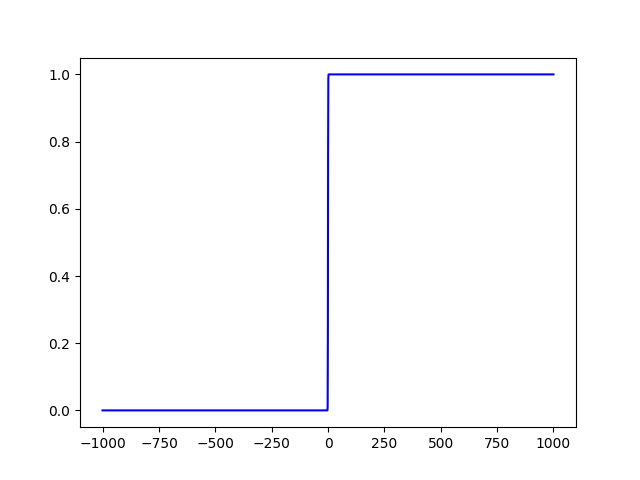
(a) Here $\zeta_{3,4}=1/2$, $\zeta_{2,4}=1/2$.

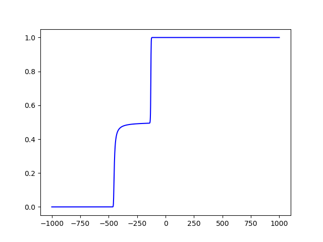
(b) Here $\zeta_{4,4}=3/16$, $\zeta_{3,4}=19/48$, $\zeta_{2,4}=5/48$ and $\zeta_{1,4}=5/16$.

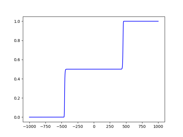
(c) Here $\zeta_{4,4}=5/16$, $\zeta_{3,4}=3/16$, $\zeta_{2,4}=3/16$ and $\zeta_{1,4}=5/16$.

Figure 1: The plots show distribution functions of $M_{1000}$ for $q=1/4\delta_{-1}+1/4\delta_{1}+1/2\delta_{0}$, $p_{4}=1$ and various $\zeta_{k,4}$, which are specified above.

Before we state the main ingredient in the proof of Theorem 3.1, let us introduce some notation. For $s\in\{1,\dots,N_{f}+1\}$, we define a stretched version of the restriction of $f(x)$ to $I_{s,n}$:

$$\widetilde{f}_{s}(x):=f((\alpha_{s}-\alpha_{s-1})x+\alpha_{s-1}),$$ (3.2)

so that

$$\widetilde{f}_{s}(0)=\widetilde{f}_{s}(1)=0,\leavevmode\nobreak\ \leavevmode\nobreak\ \widetilde{f}(x)\neq 0,\leavevmode\nobreak\ \leavevmode\nobreak\ \hbox{ for all $x\in(0,1)$.}$$ (3.3)

We also define a piece-wise linear function

$$\psi_{s,n}(x)=(q_{s,n}-q_{s-1,n}){\mathbbm{1}}(x\leq q_{s-1,n})+(q_{s,n}-x){\mathbbm{1}}({x\in[q_{s-1,n},q_{s,n}]}).$$ (3.4)

Finally, for each $n\in\operatorname{\mathbb{N}}$, we denote by $M_{n,k}$, $k\in\operatorname{\mathbb{N}}$, a family of i.i.d. random variables such that $M_{n,1}\stackrel{{\scriptstyle d}}{{=}}M_{n}$, and let $(M_{n,k;I})_{k\in\operatorname{\mathbb{N}}}$ be i.i.d. with $M_{n,1;I}\stackrel{{\scriptstyle d}}{{=}}M_{n;I}$. In addition, given any $D\geq 1$, we let $M_{n,(k);I}^{(D)}$ be the $k$-th largest element of $(M_{n,k;I})_{k\in(1,\dots,D)}$, so that

$$M_{n,(1);I}^{(D)}\leq M_{n,(2);I}^{(D)}\leq\dots\leq M_{n,(D);I}^{(D)}.$$ (3.5)

Lemma 3.2.

We have, for all $D\geq d_{0}$

$$-C_{q}\leq\mathbb{E}[\psi_{s,n}(M_{n+1})-\psi_{s,n}(M_{n})]-\sum_{k=1}^{D-1}\beta_{k,D}(\widetilde{f}_{s})\mathbb{E}\big{[}M_{n,(k+1);I_{s,n}}^{(D)}-M_{n,(k);I_{s,n}}^{(D)}\big{]}\leq C_{q}.$$ (3.6)

3.1 Proof of Theorem 3.1 assuming Lemma 3.2

Before proving Lemma 3.2, we demonstrate how it implies Theorem 3.1. Since $\operatorname{\mathrm{supp}}(q)$ is bounded we have

$$|\varphi_{n}(v)-\varphi_{n+1}(v)|\leq C_{q},\leavevmode\nobreak\ \leavevmode\nobreak\ \hbox{a.s. for $v$ with $|v|=n$.}$$

This property can be propagated up the tree, to see that

$$|\varphi_{n}(o)-\varphi_{n+1}(o)|\leq C_{q},\leavevmode\nobreak\ \leavevmode\nobreak\ \hbox{a.s.}$$

In other words, we have

$$|M_{n+1}-M_{n}|\leq C_{q},\leavevmode\nobreak\ \leavevmode\nobreak\ \hbox{a.s.}$$ (3.7)

Now, let $s\in\{1,\dots,N_{f}+1\}$ be arbitrary. The function $\psi_{s,n}$, defined in (3.4), is Lipschitz with the Lipschitz constant equal 1. Thus, (3.7) implies

$$\mathbb{E}|\psi_{s,n}(M_{n+1})-\psi_{s,n}(M_{n})|\leq C_{q}.$$ (3.8)

Combining (3.8) with Lemma 3.2 yields that for all $D\geq d_{0}$ we have

$$-2C_{q}\leq\sum_{k=1}^{D-1}\beta_{k,D}(\widetilde{f}_{s})\mathbb{E}\Big{[}M_{n,(k+1);I_{s,n}}^{(D)}-M_{n,(k);I_{s,n}}^{(D)}\Big{]}\leq 2C_{q}.$$ (3.9)

By (3.3), we know that $\widetilde{f}_{s}$ has no sign change in $[0,1]$. Thus, Proposition 2.2 can be applied to either $\widetilde{f}_{s}$ or $(-\widetilde{f}_{s})$. Hence, there is $D_{s}\geq d_{0}$ such that the coefficients $(\beta_{k,D_{s}}(\widetilde{f}_{s}))$, $k\in\{1,\dots,D_{s}-1\}$ all have the same sign and at least one of them is not zero. Fix some $k_{s}$ such that $\beta_{k_{s},D_{s}}(\widetilde{f}_{s})\neq 0$. Since all $\beta_{k,D_{s}}(\widetilde{f}_{s})$ have the same sign and because of (3.5), (3.9) implies that

$$\mathbb{E}\left[M_{n,(k_{s}+1);I_{s,n}}^{(D_{s})}-M_{n,(k_{s});I_{s,n}}^{(D_{s})}\right]\leq 2C_{q}|\beta_{k_{s},D_{s}}(\widetilde{f}_{s})|^{-1}<\infty$$ (3.10)

is bounded uniformly in $n$.

It remains to show that (3.10) implies tightness of $(M_{n;I_{s}}-\mathrm{med}(M_{n;I_{s}}))_{n\in\operatorname{\mathbb{N}}}$. Let us fix $\varepsilon>0$, and denote by $q_{n,\varepsilon}$ the $\varepsilon$-quantile of $M_{n;I_{s}}$ so that $q_{n,1/2}$ is the median of $M_{n;I_{s}}$. We have

$$\mathbb{E}\Big{[}M_{n,(k_{s}+1);I_{s,n}}^{(D_{s})}-M_{n,(k_{s});I_{s,n}}^{(D_{s})}\Big{]}\geq(q_{n,1/2}-q_{n,\varepsilon}){\mathbb{P}}\Big{[}M_{n,(k_{s});I_{s}}\leq q_{n,\varepsilon},\leavevmode\nobreak\ M_{n,(k_{s}+1);I_{s}}\geq q_{n,1/2}\Big{]}$$ (3.11)

$$=\binom{D_{s}}{k_{s}}\varepsilon^{k_{s}}(1/2)^{D_{s}-k_{s}}(q_{n,1/2}-q_{n,\varepsilon}).$$

Combining (3.11) with (3.10) yields that for all $n\in\operatorname{\mathbb{N}}$ we have

$$q_{n,1/2}-q_{n,\varepsilon}\leq\left(\binom{D_{s}}{k_{s}}\varepsilon^{k_{s}}(1/2)^{D_{s}-k_{s}}\right)^{-1}\cdot\left(2C_{q}|\beta_{k_{s},D_{s}}(\widetilde{f}_{s})|^{-1}\right)<\infty.$$ (3.12)

An analogous argument yields that

$$q_{n,(1-\varepsilon)}-q_{n,1/2}\leq\left(\binom{D_{s}}{k_{s}}(1-\varepsilon)^{D_{s}-k_{s}}(1/2)^{k_{s}}\right)^{-1}\cdot\left(2C_{q}|\beta_{k_{s},D_{s}}(\widetilde{f}_{s})|^{-1}\right)<\infty$$ (3.13)

Since $\varepsilon>0$ was arbitrary, together (3.12) and (3.13) yield that $(M_{n;I_{s}}-\mathrm{med}(M_{n;I_{s}}))_{n\in\operatorname{\mathbb{N}}}$ is tight. $\Box$

3.2 An auxiliary lemma

It is convenient to introduce the notation

$$B_{k,d}(x):=\sum_{l=k}^{d}b_{l,d}(x).$$ (3.14)

with this we can write the recursion polynomial (2.8) as

$$g(x)=\sum_{d=1}^{d_{0}}\sum_{k=1}^{d}p_{d}\zeta_{k,d}B_{k,d}(x)$$ (3.15)

and similarly for the nonlinearity $f(u)$. To prove Lemma 3.2 we need to understand how to expand the polynomial $f((\alpha_{2}-\alpha_{1})x+\alpha_{1})$ that appears in (3.2) as a weighted sum of $B_{k,d}(x)$. This is done in the next lemma. We recall the notation

$$\binom{d}{l,j,d-j-l}=\frac{d!}{l!j!(d-j-l)!}.$$ (3.16)

Lemma 3.3.

Fix a random threshold voting model $(p_{d},\zeta_{k,d})_{d\leq d_{0},k\in\{1,\dots,d\}}$ and $\alpha_{1}<\alpha_{2}\in[0,1]$. For the associated nonlinearity $f$ we have

$$f((\alpha_{2}-\alpha_{1})x+\alpha_{1}) =\sum_{d=1}^{d_{0}}\sum_{k=1}^{d}\sum_{l=0}^{k-1}\sum_{m=k-l}^{d-l}p_{d}\zeta_{k,d}\binom{d}{l,m,d-m-l}\alpha_{1}^{l}(\alpha_{2}-\alpha_{1})^{m}(1-\alpha_{2})^{d-m-l}B_{k-l,m}(x)$$ (3.17)

$$-(\alpha_{2}-\alpha_{1})x+f(\alpha_{1}).$$

Proof.

We recall that, by definition,

$$f((\alpha_{2}-\alpha_{1})x+\alpha_{1})=\sum_{d=1}^{d_{0}}\sum_{k=1}^{d}p_{d}\zeta_{k,d}B_{k,d}((\alpha_{2}-\alpha_{1})x+\alpha_{1})-(\alpha_{2}-\alpha_{1})x-\alpha_{1}.$$ (3.18)

Thus, to prove (3.17) it is enough to show that for all $d\in\operatorname{\mathbb{N}}$, $k\leq d$ we have

$$B_{k,d}((\alpha_{2}-\alpha_{1})x+\alpha_{1})=\sum_{l=0}^{k-1}\sum_{m=k-l}^{d-l}\!\binom{d}{l,m,d-m-l}\alpha_{1}^{l}(\alpha_{2}-\alpha_{1})^{m}(1-\alpha_{2})^{d-m-l}B_{k-l,m}(x)+B_{k,d}(\alpha_{1}).$$ (3.19)

We do this by a direct computation. We start by looking at the stretched version of $b_{j,d}$:

$$b_{j,d}((\alpha_{2}-\alpha_{1})x+\alpha_{1})=\binom{d}{j}((\alpha_{2}-\alpha_{1})x+\alpha_{1})^{j}(1-(\alpha_{2}-\alpha_{1})x-\alpha_{1})^{d-j}$$ (3.20)

$$=\binom{d}{j}\Big{[}\sum_{l=0}^{j}\binom{j}{l}(\alpha_{2}-\alpha_{1})^{l}x^{l}\alpha_{1}^{j-l}\Big{]}\Big{[}\sum_{m=0}^{d-j}\binom{d-j}{m}(1-\alpha_{2})^{d-j-m}(\alpha_{2}-\alpha_{1})^{m}(1-x)^{m}\Big{]}$$

$$=\sum_{l=0}^{j}\sum_{m=0}^{d-j}\binom{d}{j}\binom{j}{l}\binom{d-j}{m}(\alpha_{2}-\alpha_{1})^{l+m}(1-\alpha_{2})^{d-j-m}\alpha_{1}^{j-l}x^{l}(1-x)^{m}$$

$$=\sum_{l=0}^{j}\sum_{m=0}^{d-j}\binom{d}{j-l,l+m,d-j-m}b_{l,l+m}(x)(\alpha_{2}-\alpha_{1})^{l+m}(1-\alpha_{2})^{d-j-m}\alpha_{1}^{j-l}$$

$$=\sum_{l=0}^{j}\sum_{m=0}^{d-j}\binom{d}{l,j-l+m,d-j-m}b_{j-l,j-l+m}(x)(\alpha_{2}-\alpha_{1})^{j-l+m}(1-\alpha_{2})^{d-j-m}\alpha_{1}^{l}.$$

The next to last step above uses the definition of $b_{l,l+m}$ as well as the relation

$$\binom{d}{j}\binom{j}{l}\binom{d-j}{m}\Big{[}\binom{l+m}{l}\Big{]}^{-1} =\frac{d!}{j!(d-j)!}\frac{j!}{l!(j-l)!}\frac{(d-j)!}{m!(d-j-m)!}\frac{l!m!}{(l+m)!}$$ (3.21)

$$=\frac{d!}{(j-l)!(d-j-m)!(l+m)!}=\binom{d}{j-l,l+m,d-j-m}.$$

Plugging (3.20) into the definition (3.14) of $B_{k,d}$ yields

$$B_{k,d}((\alpha_{2}-\alpha_{1})x+\alpha_{1})=\sum_{j=k}^{d}b_{j,d}((\alpha_{2}-\alpha_{1})(x)+\alpha_{1})$$ (3.22)

$$=\sum_{j=k}^{d}\sum_{l=0}^{j}\sum_{m=0}^{d-j}\binom{d}{l,j-l+m,d-j-m}b_{j-l,j-l+m}(x)(\alpha_{2}-\alpha_{1})^{j-l+m}(1-\alpha_{2})^{d-j-m}\alpha_{1}^{l}.$$

Exchanging the order of summation of the sums over $j$ and $l$ and changing the index of summation of the third sum to $\widehat{m}=j-l+m$ yields

$$B_{k,d}((\alpha_{2}-\alpha_{1})x+\alpha_{1})=\sum_{l=k+1}^{d}\sum_{j=l}^{d}\sum_{m=j-l}^{d-l}\binom{d}{l,m,d-m-l}b_{j-l,m}(x)(\alpha_{2}-\alpha_{1})^{m}(1-\alpha_{2})^{d-m-l}\alpha_{1}^{l}$$ (3.23)

$$\qquad+\sum_{l=0}^{k}\sum_{j=k}^{d}\sum_{m=j-l}^{d-l}\binom{d}{l,m,d-m-l}b_{j-l,m}(x)(\alpha_{2}-\alpha_{1})^{m}(1-\alpha_{2})^{d-m-l}\alpha_{1}^{l}.$$

Exchanging the order of summation of the sums over $m$ and $j$ yields

$$B_{k,d}((\alpha_{2}-\alpha_{1})x+\alpha_{1}) =\sum_{l=k+1}^{d}\sum_{m=0}^{d-l}\sum_{j=l}^{m+l}\binom{d}{l,m,d-m-l}b_{j-l,m}(x)(\alpha_{2}-\alpha_{1})^{m}(1-\alpha_{2})^{d-m-l}\alpha_{1}^{l}$$ (3.24)

$$+\sum_{l=0}^{k}\sum_{m=k-l}^{d-l}\sum_{j=k}^{m+l}\binom{d}{l,m,d-m-l}b_{j-l,m}(x)(\alpha_{2}-\alpha_{1})^{m}(1-\alpha_{2})^{d-m-l}\alpha_{1}^{l}.$$

Now, switching the summation over $j$ to $\hat{j}=j-l$ and dropping the hat gives

$$B_{k,d}((\alpha_{2}-\alpha_{1})x+\alpha_{1}) =\sum_{l=k+1}^{d}\sum_{m=0}^{d-l}\sum_{j=0}^{m}\binom{d}{l,m,d-m-l}b_{j,m}(x)(\alpha_{2}-\alpha_{1})^{m}(1-\alpha_{2})^{d-m-l}\alpha_{1}^{l}$$ (3.25)

$$+\sum_{l=0}^{k}\sum_{m=k-l}^{d-l}\sum_{j=k-l}^{m}\binom{d}{l,m,d-m-l}b_{j,m}(x)(\alpha_{2}-\alpha_{1})^{m}(1-\alpha_{2})^{d-m-l}\alpha_{1}^{l}.$$

Next, we use (2.17) in the first sum in (3.25) and the definition (3.14) of $B_{k-l,m}$ in the second, to obtain

$$B_{k,d}((\alpha_{2}-\alpha_{1})x+\alpha_{1}) =\sum_{l=k+1}^{d}\sum_{m=0}^{d-l}\binom{d}{l,m,d-m-l}(\alpha_{2}-\alpha_{1})^{m}(1-\alpha_{2})^{d-m-l}\alpha_{1}^{l}$$ (3.26)

$$+\sum_{l=0}^{k}\sum_{m=k-l}^{d-l}\binom{d}{l,m,d-m-l}\alpha_{1}^{l}(\alpha_{2}-\alpha_{1})^{m}(1-\alpha_{2})^{d-m-l}B_{k-l,m}(x).$$

The summation over $m$ in the first sum in (3.26) can be re-written as

$$\sum_{m=0}^{d-l}\binom{d}{l,m,d-m-l}(\alpha_{2}-\alpha_{1})^{m}(1-\alpha_{2})^{d-m-l}=\sum_{m=0}^{d-l}\frac{d!(d-l)!}{l!m!(d-m-l)!(d-l)!}(\alpha_{2}-\alpha_{1})^{m}(1-\alpha_{2})^{d-m-l}$$ (3.27)

$$=\frac{d!}{l!(d-l)!}(1-\alpha_{1})^{d-l}=\binom{d}{l}(1-\alpha_{1})^{d-l}.$$

Furthermore, as $B_{0,m}(x)\equiv 1$ because of (2.17), the $l=k$ summand in the second sum in (3.26) can be written as

$$\sum_{m=0}^{d-k}\binom{d}{k,m,d-m-k}\alpha_{1}^{k}(\alpha_{2}-\alpha_{1})^{m}(1-\alpha_{2})^{d-m-k}B_{0,m}(x)$$ (3.28)

$$=\sum_{m=0}^{d-k}\frac{d!(d-k)!}{k!m!(d-m-k)!(d-k)!}\alpha_{1}^{k}(\alpha_{2}-\alpha_{1})^{m}(1-\alpha_{2})^{d-m-k}=\binom{d}{k}\alpha_{1}^{k}(1-\alpha_{1})^{d-k}.$$

Using (3.27) and (3.28) in (3.26) leads to

$$B_{k,d}((\alpha_{2}-\alpha_{1})x+\alpha_{1})$$

$$=\sum_{l=k}^{d}\binom{d}{l}\alpha_{1}^{l}(1-\alpha_{1})^{d-l}+\sum_{l=0}^{k-1}\sum_{j=k-l}^{d-l}\binom{d}{l,j,d-j-l}\alpha_{1}^{l}(\alpha_{2}-\alpha_{1})^{j}(1-\alpha_{2})^{d-j-l}B_{k-l,j}(x)$$

$$=B_{k,d}(\alpha_{1})+\sum_{l=0}^{k-1}\sum_{m=k-l}^{d-l}\binom{d}{l,m,d-m-l}\alpha_{1}^{l}(\alpha_{2}-\alpha_{1})^{m}(1-\alpha_{2})^{d-m-l}B_{k-l,m}(x).$$

This proves (3.19) finishing the proof of (3.17). ∎

3.3 Proof of Lemma 3.2

Here, we prove Lemma 3.2, finishing the proof to Theorem 3.1. Let us consider a collection of independent random variables $(Z,(M_{n,k})_{k\in\operatorname{\mathbb{N}}}$, $(X_{k})_{k\in\operatorname{\mathbb{N}}})$ such that

$$\mathbb{P}[Z=d]=p_{d},$$ (3.29)

$$M_{n,k}\stackrel{{\scriptstyle d}}{{=}}M_{n},$$

$$X_{k}\sim q,$$

and also a random variable $L$ independent of $(M_{n,k},X_{k})_{k\in\operatorname{\mathbb{N}}}$ with

$$\mathbb{P}[L=k|Z=d]=\zeta_{k,d}.$$ (3.30)

Observe that the same reasoning giving the recursion (2.7) yields a recursion relation

$$M_{n+1}\stackrel{{\scriptstyle d}}{{=}}\sum_{d=1}^{d_{0}}{\mathbbm{1}}({Z=d})(M_{n,1}+X_{1},\dots,M_{n,d}+X_{d})_{(L)}.$$ (3.31)

Recall that the Lipschitz function $\psi_{s,n}(x)$ that appears in the statement of Lemma 3.2 is defined by (3.4). Since there is only one non-zero term in the sum in the right side of (3.31), the recursion (3.31) immediately implies that

$$\mathbb{E}[\psi_{s,n}(M_{n+1})] =\mathbb{E}\Big{[}\psi_{s,n}\Big{(}\sum_{d=1}^{d_{0}}{\mathbbm{1}}({Z=d})(M_{n,1}+X_{1},\dots,M_{n.d}+X_{d})_{(L)}\Big{)}\Big{]}$$ (3.32)

$$=\mathbb{E}\Big{[}\sum_{d=1}^{d_{0}}{\mathbbm{1}}({Z=d})\psi_{s,n}\left((M_{n,1}+X_{1},\dots,M_{n,d}+X_{d})_{(L)}\right)\Big{]}$$

$$\leq\mathbb{E}\Big{[}\sum_{d=1}^{d_{0}}{\mathbbm{1}}({Z=d})\psi_{s,n}\left(M_{n,(L)}^{(d)}\right)\Big{]}\!+\mathbb{E}\Big{[}\max_{k\in\{1,\dots,d_{0}\}}X_{k}\Big{]}\leq\sum_{d=1}^{d_{0}}\sum_{k=1}^{d}p_{d}\zeta_{k,d}\mathbb{E}[\psi_{s,n}(M_{n,(k)}^{(d)})]+C_{q}.$$

The third step used the fact that $\psi_{s,n}$ is Lipschitz with Lipschitz constant $1$ and the last step used (1.6) and (3.29).

Let us write

$$\psi_{s,n}(M_{n})=(q_{s,n}-q_{s-1,n}){\mathbbm{1}}(M_{n}\leq q_{s-1,n})+(q_{s,n}-M_{n}){\mathbbm{1}}({M_{n}\in[q_{s-1,n},q_{s,n}]}).$$ (3.33)

and take the expectation:

$$\mathbb{E}[\psi_{s,n}(M_{n})]=\alpha_{s-1}(q_{s,n}-q_{s-1,n})+(\alpha_{s}-\alpha_{s-1})\mathbb{E}[q_{s,n}-M_{n;I_{s,n}}].$$ (3.34)

An analogous argument using $\min_{k\in\{1,\dots,d_{0}\}}X_{k}$ and subtracting (3.34) from both sides of (3.32) yields

$$\mathbb{E}[\psi_{s,n}(M_{n+1})-\psi_{s,n}(M_{n})]-C_{q}$$ (3.35)

$$\leq\sum_{d=1}^{d_{0}}\sum_{k=1}^{d}p_{d}\zeta_{k,d}\mathbb{E}[\psi_{s,n}(M_{n,(k)}^{(d)})]-\alpha_{s-1}(q_{s,n}-q_{s-1,n})-(\alpha_{s}-\alpha_{s-1})\mathbb{E}[q_{s,n}-M_{n;I_{s},n}]$$

$$\leq\mathbb{E}[\psi_{s,n}(M_{n+1})-\psi_{s,n}(M_{n})]+C_{q}.$$

By decomposing with regard to how many of the $M_{n,k}$ are in $(-\infty,q_{s-1,n}]$, in $[q_{s-1,n},q_{s,n}]$ and in $[q_{s,n},\infty)$, respectively, we get from (3.33)

$$\mathbb{E}\left[\psi_{s,n}\left(M_{n,(k)}^{(d)}\right)\right] =\sum_{l=0}^{k-1}\sum_{j=k-l}^{d-l}\binom{d}{l,j,d-j-l}\alpha_{s-1}^{l}(\alpha_{s}-\alpha_{s-1})^{j}(1-\alpha_{s})^{d-l-j}\mathbb{E}[q_{s,n}-M_{n,(k-l);I_{s,n}}^{(j)}]$$ (3.36)

$$+\sum_{l=k}^{d}\sum_{j=0}^{d-l}\binom{d}{l,j,d-j-l}\alpha_{s-1}^{l}(\alpha_{s}-\alpha_{s-1})^{j}(1-\alpha_{s})^{d-l-j}(q_{s,n}-q_{s-1,n}).$$

The second sum in the right side can be simplified by writing

$$\sum_{j=0}^{d-l}\binom{d}{l,j,d-j-l}(\alpha_{s}-\alpha_{s-1})^{j}(1-\alpha_{s})^{d-l-j}$$ (3.37)

$$=\sum_{j=0}^{d-l}\frac{d!(d-l)!}{l!j!(d-j-l)!(d-l)!}(\alpha_{s}-\alpha_{s-1})^{j}(1-\alpha_{s})^{d-l-j}=\binom{d}{l}(1-\alpha_{s-1})^{d-l}.$$

Let us consider the term in the second line of (3.35):

$$\Sigma_{{s,n}}:=\sum_{d=1}^{d_{0}}\sum_{k=1}^{d}p_{d}\zeta_{k,d}\mathbb{E}[\psi_{s,n}(M_{n,(k)}^{(d)})]-\alpha_{s-1}(q_{s,n}-q_{s-1,n})-(\alpha_{s}-\alpha_{s-1})\mathbb{E}[q_{s,n}-M_{n;I_{s},n}].$$ (3.38)

Note that (3.35) says

$$\Big{|}\mathbb{E}[\psi_{s,n}(M_{n+1})-\psi_{s,n}(M_{n})]-\Sigma_{s,n}\Big{|}\leq C_{q}.$$ (3.39)

Thus, the conclusion of Lemma 3.2 will follow if we show that

$$\Sigma_{s,n}=\sum_{k=1}^{D-1}\beta_{k,D}(\widetilde{f}_{s})\mathbb{E}\big{[}M_{n,(k+1);I_{s,n}}^{(D)}-M_{n,(k);I_{s,n}}^{(D)}\big{]}.$$ (3.40)

Using (3.36) and (3.37) in the definition (3.38) of $\Sigma_{s,n}$, we can re-write that sum as

$$\Sigma_{s,n} =\sum_{d=1}^{d_{0}}\sum_{k=1}^{d}\sum_{l=0}^{k-1}\sum_{j=k-l}^{d-l}p_{d}\zeta_{k,d}\binom{d}{l,j,d-j-l}\alpha_{s-1}^{l}(\alpha_{s}-\alpha_{s-1})^{j}(1-\alpha_{s})^{d-l-j}\mathbb{E}[q_{s,n}-M_{n,(k-l);I_{s,n}}^{(j)}]$$ (3.41)

$$+(q_{s,n}-q_{s-1,n})\Big{(}\sum_{d=1}^{d_{0}}\sum_{k=1}^{d}p_{d}\zeta_{k,d}\sum_{l=k}^{d}\binom{d}{l}\alpha_{s-1}^{l}(1-\alpha_{s-1})^{d-l}-\alpha_{s-1}\Big{)}$$

$$-(\alpha_{s}-\alpha_{s-1})\mathbb{E}[q_{s,n}-M_{n;I_{s,n}}]$$

$$=\sum_{d=1}^{d_{0}}\sum_{k=1}^{d}\sum_{l=0}^{k-1}\sum_{j=k-l}^{d-l}p_{d}\zeta_{k,d}\binom{d}{l,j,d-j-l}\alpha_{s-1}^{l}(\alpha_{s}-\alpha_{s-1})^{j}(1-\alpha_{s})^{d-l-j}\mathbb{E}[q_{s,n}-M_{n,(k-l);I_{s,n}}^{(j)}]$$

$$\qquad-(\alpha_{s}-\alpha_{s-1})\mathbb{E}[q_{s,n}-M_{n;I_{s,n}}].$$

The second step above used the identity

$$\sum_{d=1}^{d_{0}}\sum_{k=1}^{d}p_{d}\zeta_{k,d}\sum_{l=k}^{d}\binom{d}{l}\alpha_{s-1}^{l}(1-\alpha_{s-1})^{d-l}-\alpha_{s-1}=f(\alpha_{s-1})=0.$$

On the other hand, by using Lemma 3.3 as well as $f(\alpha_{s-1})=0$ we see that

$$\widetilde{f}_{s}(x)=\sum_{d=1}^{d_{0}}\sum_{k=1}^{d}\sum_{l=0}^{k-1}\sum_{j=k-l}^{d-l}p_{d}\zeta_{k,d}\binom{d}{l,j,d-j-l}\alpha_{s-1}^{l}(\alpha_{s}-\alpha_{s-1})^{j}(1-\alpha_{s})^{d-j-l}B_{k-l,j}(x)$$ (3.42)

$$\qquad-(\alpha_{s}-\alpha_{s-1})x.$$

Comparing (3.41) to (3.42) we see that the coefficient in front of $B_{k-l,j}(x)$ in the expression for $\widetilde{f}_{s}$ equals the coefficient in front of $\mathbb{E}[q_{s,n}-M_{n,(k-l);I_{s,n}}^{(j)}]$ in $\Sigma_{s,n}$. Thus to show that for all $D\geq d_{0}$ there are coefficients $\beta_{k,D,s}$ such that

$$\Sigma_{s,n}=\sum_{k=1}^{D}\beta_{k,D,s}\mathbb{E}[q_{s,n}-M_{n,(k);I_{s,n}}^{(D)}]\quad\text{and}\quad\widetilde{f}_{s}(x)=\sum_{k=1}^{D}\beta_{k,D,s}B_{k,D}(x)$$ (3.43)

it is enough to show that there is a family of multi-linear functions

$$f_{k,d,D}:\operatorname{\mathbb{R}}^{D}\to\operatorname{\mathbb{R}},\leavevmode\nobreak\ \leavevmode\nobreak\ D\geq 1,\leavevmode\nobreak\ \leavevmode\nobreak\ d\in\{1,\dots,D\},\leavevmode\nobreak\ \leavevmode\nobreak\ k\in\{1,\dots,d\},$$

such that

$$B_{k,d} =f_{k,d,D}(B_{1,D},\dots,B_{D,D}),$$ (3.44)

and

$$\mathbb{E}[q_{s,n}-M_{n,(k);I_{s,n}}^{(d)}] =f_{k,d,D}\left(\mathbb{E}[q_{s,n}-M_{n,(1);I_{s,n}}^{(D)}],\dots,\mathbb{E}[q_{s,n}-M_{n,(D);I_{s,n}}^{(D)}]\right).$$ (3.45)

Since a composition of multilinear functions is multilinear itself, it is enough to show this for $D=d+1$.

To this end, first note that, using (2.19) and the definition of $B_{k,d}$, we have for all $d\in\operatorname{\mathbb{N}}$, $k\leq d$

$$B_{k,d}(x)=\sum_{j=k}^{d}b_{j,d}(x)=\sum_{j=k}^{d}\Big{[}\frac{d-j+1}{d+1}b_{j,d+1}(x)+\frac{j+1}{d+1}b_{j+1,d+1}(x)\Big{]}$$ (3.46)

$$=\sum_{j=k}^{d}\Big{[}b_{j,d+1}(x)-\frac{j}{d+1}b_{j,d+1}(x)+\frac{j+1}{d+1}b_{j+1,d+1}(x)\Big{]}=\sum_{j=k}^{d}b_{j,d+1}(x)-\frac{k}{d+1}b_{k,d+1}(x)+b_{d+1,d+1}(x)$$

$$=B_{k,d+1}(x)-\frac{k}{d+1}[B_{k,d+1}(x)-B_{k+1,d+1}(x)]=\frac{d+1-k}{d+1}B_{k,d+1}(x)+\frac{k}{d+1}B_{k+1,d+1}(x).$$

On the other hand, for any collection of i.i.d. random variables $X_{k}$, $k\in{\mathbb{N}}$, so that $X_{1}$ has a continuous density, and any $d\geq 1$, $1\leq k\leq d$, we have the identity

$${\mathbb{E}}[X^{(d)}_{(k)}]=\frac{k}{d+1}{\mathbb{E}}[X^{(d+1)}_{(k+1)}]+\frac{d+1-k}{d+1}{\mathbb{E}}[X^{(d+1)}_{(k)}],$$ (3.47)

as can be seen simply by adding $X_{d+1}$ to the collection $\{X_{1},\dots,X_{d}\}$ and looking at whether $X_{d+1}$ is to the left or to the right of $X_{(k)}^{(d)}$. Applying (3.47) to $M_{n,k;I_{s,n}}$ shows that for all $d\in\operatorname{\mathbb{N}}$, $k\leq d$ we have

$$\mathbb{E}[q_{s,n}-M_{n,(k);I_{s,n}}^{(d)}]=\frac{k}{d+1}\mathbb{E}[q_{s,n}-M_{n,(k+1);I_{s,n}}^{(d+1)}]+\frac{d+1-k}{d+1}\mathbb{E}[q_{s,n}-M_{n,(k);I_{s,n}}^{(d+1)}].$$ (3.48)

As mentioned above, comparing (3.46) to (3.48) yields that for all $D\geq d_{0}$ there are coefficients $\beta_{k,D,s}$ such that (3.43) holds. As we also have

$$b_{k,D}=B_{k,D}-B_{k+1,D},$$

and

$$\mathbb{E}[M_{n,(k+1);I_{s,n}}^{(D)}-M_{n,(k);I_{s,n}}^{(D)}]=\mathbb{E}[q_{s,n}-M_{n,(k);I_{s,n}}^{(D)}]-\mathbb{E}[q_{s,n}-M_{n,(k+1);I_{s,n}}^{(D)}],$$

equation (3.43) implies that for all $s\in\{1,\dots,N_{f}+1\}$ and $D\geq d_{0}$ we have

$$\Sigma_{s,n}=\sum_{k=1}^{D-1}\beta_{k,D}(\widetilde{f}_{s})\mathbb{E}\left[M_{n,(k+1);I_{s,n}}^{(D)}-M_{n,(k);I_{s,n}}^{(D)}\right].$$ (3.49)

Recalling (3.35) we see that (3.49) implies the statement of Lemma 3.2, finishing the proof. $\Box$

3.4 The binary-ternary case as an example

In this section we will look at the threshold voting models with $p_{2}=p$, $p_{3}=(1-p)$ for $p\in[0,1]$ and $\zeta_{2,3}=\zeta_{2,2}=1$. In other words, a parent who has three children is assigned the middle one of their values, while a parent with two children gets the larger value of the two.

There are several reasons to look at these models: they have an additional probabilistic interpretation, they are convenient for showing that we can get a slightly stronger result than Theorem 3.1 with probabilistic means, and for $p<1/2$ they are example for which the nonlinearity has the single additional zero $1/(2(1-p))$ in $(0,1)$ as well as $f^{\prime}(0)<0$, $f^{\prime}(1)<0$. In Section 4, we will use analytic methods to show that for such nonlinearities $f$ the sequence $(M_{n}-\mathrm{med}(M_{n}))_{n\in\operatorname{\mathbb{N}}}$ is tight.

Let us mention an alternative probabilistic interpretation for that voting model. Let ${\cal T}_{n}$ be the genealogical tree of the underlying BRW up to generation $n$ and $\mathbf{T}_{n}^{(2)}:=\{(T_{n},o)\subseteq{\cal T}_{n}:T_{n}\ \text{binary}\}$ be the collection of rooted full binary subtrees of ${\cal T}_{n}$ with root $o$ and depth $n$. Given a binary subtree $(T_{n},o)\in\mathbf{T}_{n}^{(2)}$, we define

$$M_{n,T_{n}}:=\max_{v\in T_{n}:|v|=n}S_{v},$$

as the maximum at time $n$ along $T_{n}$. Finally, we set

$$\widetilde{M}_{n}:=\min_{(T_{n},o)\in\mathbf{T}_{n}^{(2)}}M_{n,T_{n}}$$ (3.50)

to be the smallest maximum along all binary subtrees of ${\cal T}_{n}$. Analogously, we define

$$\widehat{M}_{n}:=\max_{(T_{n},o)\in\mathbf{T}_{n}^{(2)}}\min_{v\in T_{n}:|v|=n}S_{v}$$ (3.51)

as the largest minimum along all binary subtrees.

Let us make a couple of simple observations. First, it follows from the definition above that

$$M_{n}=\widetilde{M}_{n}.$$ (3.52)

Furthermore, in the case of purely ternary branching $p=0$, we have

$$M_{n}=\widetilde{M}_{n}=\widehat{M}_{n}.$$ (3.53)

In particular, it follows that, for $q$ symmetric and purely ternary branching, the distribution of $M_{n}$ is symmetric for all $n\geq 1$, and

$$\mathbb{E}[M_{n}]=\mathrm{med}(M_{n})=0.$$ (3.54)

While the description of $M_{n}$ as the smallest maximum of all binary subtrees of ${\cal T}_{n}$ is quite nice and links the study of $M_{n}$ to the study of the maximum of BRWs, we were unable to use it to gain any insights into the distribution of $M_{n}$. One of the reasons for this is that while we have very precise control of $\mathbb{P}[M_{n,T_{n}}\leq t]$ for $T_{n}$ a fixed binary subtree of ${\cal T}_{n}$, there are $3^{2^{n}-1}$ binary subtrees of ${\cal T}_{n}$, which are far too many for a first moment method to work. Of course, many of these binary subtrees share many vertices. For example, for any given binary subtree $T_{n}$ of ${\cal T}_{n}$ there are at least $3^{2^{n-1}}$ binary subtrees $\widetilde{T}_{n}$ such that $\{v\in T_{n}:|v|=n-1\}=\{v\in\widetilde{T}_{n}:|v|=n-1\}$. The issue we could not overcome is that we do not know how to properly use the fact that many of the maxima along the binary subtrees are strongly correlated.

The rest of this section is devoted to the subsequential tightness of $(M_{n})_{n\in\operatorname{\mathbb{N}}}$ in the fully ternary case.

Theorem 3.4.

In addition to our standing assumptions (1.6) on $q$, assume that $q$ is symmetric. Consider the voting model with $p_{3}=1$ and $\zeta_{2,3}=1$. There is a subset $I\subseteq\operatorname{\mathbb{N}}$ of the natural numbers such that $(M_{n})_{n\in I}$ is tight and

$$\liminf_{n\to\infty}\frac{I\cap\{1\dots,n\}}{n}>0.$$ (3.55)

Let us first outline the proof of this theorem. It relies on the voting model interpretation of $M_{n}$. Observe that in the symmetric case we have

$$-M_{n;I_{1}}\stackrel{{\scriptstyle d}}{{=}}M_{n;I_{2}}\stackrel{{\scriptstyle d}}{{=}}|M_{n}|.$$

Thus, Theorem 3.1 implies that $(|M_{n}|-\mathrm{med}(|M_{n}|))_{n\in\operatorname{\mathbb{N}}}$ is tight. Thus, for the full tightness of $M_{n}$ it is enough to show that there are $\varepsilon,C>0$ such that for all $n\in\operatorname{\mathbb{N}}$ we have

$$\mathbb{P}[|M_{n}|\leq C]\geq\varepsilon.$$ (3.56)

We have not been able to prove (3.56) by purely probabilistic means. Instead we show by contradiction that if

$$\liminf_{n\to\infty}\big{[}\mathrm{med}(|M_{n}|)\big{]}=+\infty,$$ (3.57)

it is too likely for a particle $v$ with $S_{v}\approx 0$ to be voted to the top, making $\mathbb{P}[M_{n}\approx 0]$ too large. To see this, first note that $S_{v}$ is voted to the top if and only if at each ancestor $v_{k}$, $|v_{k}|=k$, of $v$ we have

$$\max_{w\in D_{1}(v_{k})\setminus\{v_{k+1}\}}\varphi_{n}(w)\geq S_{v}\geq\min_{w\in D_{1}(v_{k})\setminus\{v_{k+1}\}}\varphi_{n}(w).$$ (3.58)

Suppose now that (3.57) holds and take $N$ sufficiently large. Because of (3.57), we have

$$\mathrm{med}(|M_{n}|)\gg 100N,$$ (3.59)

for all $n$ sufficiently large. There exists $\eta_{N}>0$ so that with the probability $(1-\eta_{N})^{n}$, we have, for all $k\leq n$, both

$$\max_{w\in D_{1}(v_{k})\setminus\{v_{k+1}\}}|S_{w}-S_{v_{k}}|\leq N,$$ (3.60)

and

$$\max_{k\leq n}|S_{v}-S_{v_{k}}|\leq N.$$ (3.61)

We may also choose $\eta_{N}$ so that

$$\eta_{N}\to 0,\leavevmode\nobreak\ \leavevmode\nobreak\ \hbox{as $N\to+\infty$.}$$ (3.62)

Note that, under the conditions (3.60) and (3.61), (3.58) holds if

$$\max_{w\in D_{1}(v_{k})\setminus\{v_{k+1\}}}[\varphi_{n}(w)-S_{w}]\geq 2N\quad\text{and}\min_{w\in D_{1}(v_{k})\setminus\{v_{k+1\}}}[\varphi_{n}(w)-S_{w}]\leq-2N.$$ (3.63)

By construction, we have

$$\varphi_{n}(w)-S_{w}\stackrel{{\scriptstyle d}}{{=}}M_{n-|w|}.$$ (3.64)

If (3.59) holds for all $k\leq n$, the tightness of $(|M_{n}|-\mathrm{med}(|M_{n}|))_{n\in\operatorname{\mathbb{N}}}$ and (3.64) ensure that the probability of the event in (3.63) is roughly equal to $2(1/2-\varepsilon_{N})^{2}$ with

$$\lim_{N\to+\infty}\varepsilon_{N}=0.$$ (3.65)

Thus, overall we have

$$\mathbb{P}[M_{n}\in[-N,N]]=3^{n}\mathbb{P}[S_{v}\in[-N,N],M_{n}=S_{v}]\approx 3^{n}(1-\eta_{N})^{n}2^{n}(1/2-\varepsilon_{N})^{2n},$$

which is bigger than $1$ for $\eta_{N}$, $\varepsilon_{N}$ small enough, which yields a contradiction to (3.59). In the actual proof of Theorem 3.4 we will need to strengthen the lower bound so that it still holds (and is bigger than 1) if every once in a while we do not have $\mathrm{med}(|M_{k}|)\gg 100N$.

Proof of Theorem 3.4

Given

$$K>C_{q},$$ (3.66)

sufficiently large, we set

$$I_{K}:=\{n\in\operatorname{\mathbb{N}}_{0}:\mathrm{med}(|M_{n}|)\leq K\}.$$

We will put further restrictions on $K$, in addition to (3.66), during the proof, keeping it as large as needed, but independent of $n$.

As we have mentioned, the symmetry of $M_{n}$ and Theorem 3.1 imply that $(|M_{n}|-\mathrm{med}(|M_{n}|))_{n\in\operatorname{\mathbb{N}}}$ is tight. Thus, the family $(M_{n})_{n\in I_{4K}}$ is tight and it is enough to prove that

$$\liminf_{n\to\infty}\frac{I_{4K}\cap\{0,\dots,n-1\}}{n}>0.$$ (3.67)

First, we note that for $K$ big enough we have

$$\mathbb{P}[M_{k}\leq-3K]=\mathbb{P}[M_{k}\geq 3K]\geq 1/2-1/200,\leavevmode\nobreak\ \leavevmode\nobreak\ \hbox{ for all $k\in I_{4K}^{c}$}.$$ (3.68)

This is true, since, using the symmetry of $M_{n}$, we can write

$$\mathbb{P}[M_{k}\geq 3K]=\frac{1}{2}\mathbb{P}[|M_{k}|\geq 3K]\geq\frac{1}{2}\mathbb{P}\left[\left||M_{k}|-\mathrm{med}(|M_{k}|)\right|\leq K\right]\geq\frac{1}{2}-\frac{1}{200},\leavevmode\nobreak\ \leavevmode\nobreak\ \hbox{ for all $k\in I_{4K}^{c}$},$$ (3.69)

as long as $K$ is chosen to be large enough, but independent of $n$. The last step in (3.69) used the tightness of $(|M_{n}|-\mathrm{med}(|M_{n}|))_{n\in\operatorname{\mathbb{N}}}$.

Next, we set

$$\widetilde{I}_{4K,n}:=\{k\in\{0,\dots,n-1\}:n-k-1\in I_{4K}\}.$$ (3.70)

Finally, we fix a vertex $v$ with $|v|=n$ and define the event

$$A_{n,\delta_{0}}(v):=\left\{|S_{v_{k}}-S_{v}|\leq K\hbox{ for all $k\leq n$}\hbox{ and }|S_{v}-S_{v_{k}}|\leq\delta_{0}\hbox{ for all }k\in\widetilde{I}_{4K,n}\right\}.$$ (3.71)

Here, $\delta_{0}>0$ is chosen so that

$$\int_{(-\delta_{0},\delta_{0})^{c}}q(x)\mathop{}\!dx>0,\inf_{x\in[-\delta_{0},\delta_{0}]}\int_{-\delta_{0}}^{\delta_{0}}q(y-x)\mathop{}\!dy>0.$$ (3.72)

To see that such choice of $\delta_{0}>0$ is possible, we use the continuity of $q(x)$ to find $\delta_{0}>0$ such that

$$\int_{[-\delta_{0},\delta_{0}]^{c}}q(y)\mathop{}\!dy=\frac{1}{2}.$$ (3.73)

As $q(x)$ is symmetric, this is equivalent to

$$\int_{\delta_{0}}^{\infty}q(y)\mathop{}\!dy=\frac{1}{4},\leavevmode\nobreak\ \leavevmode\nobreak\ \int_{0}^{\delta_{0}}q(y)\mathop{}\!dy=\frac{1}{4}.$$ (3.74)

Note that then for each $x\in[0,\delta_{0}]$ we have

$$\int_{-\delta_{0}}^{\delta_{0}}q(y-x)\mathop{}\!dy=\int_{-\delta_{0}-x}^{\delta_{0}-x}q(y)\mathop{}\!dy\geq\int_{-\delta_{0}}^{0}q(y)\mathop{}\!dy=\frac{1}{4}.$$ (3.75)

By symmetry, we also have, for each $x\in[-\delta_{0},0]$:

$$\int_{-\delta_{0}}^{\delta_{0}}q(y-x)\mathop{}\!dy=\int_{-\delta_{0}-x}^{\delta_{0}-x}q(y)\mathop{}\!dy\geq\int_{0}^{\delta_{0}}q(y)\mathop{}\!dy=\frac{1}{4}.$$ (3.76)

Summarizing (3.73) and (3.75)–(3.76), we have chosen $\delta_{0}>0$ such that (3.72) holds.

Using the exchangeability of the vertices in the same generation of ${\cal T}_{n}$ yields that

$$\mathbb{P}[M_{n}\in[-K,K]] =\sum_{w\in{\cal T}_{n}:|w|=n}\mathbb{P}[M_{n}\in[-K,K],S_{w}=M_{n}]=3^{n}\mathbb{P}[M_{n}=S_{v},S_{v}\in[-K,K]]$$

$$\geq 3^{n}\mathbb{P}\left[A_{n,\delta_{0}}(v),\ \forall_{k\in\{0,\dots,n-1\}}\varphi_{n}(v_{k})=\varphi_{n}(v_{k+1})\in[-K,K]\right].$$ (3.77)

For $k\in\{0,\dots,n-1\}$ let $D_{1}(v_{k})=\{v_{k+1},w_{1}(k),w_{2}(k)\}$ denote the direct descendants of $v_{k}$. Using the exchangeability of $w_{1}(k)$, $w_{2}(k)$ yields that we can continue from (3.4) to get

$$\mathbb{P}[M_{n}\in[-K,K]] \geq 6^{n}\mathbb{P}\left[A_{n,\delta_{0}}(v),\forall_{k\leq n-1}\varphi_{n}(w_{1}(k))\leq\varphi_{n}(v_{k})\leq\varphi_{n}(w_{2}(k))\right]$$

$$=6^{n}\mathbb{P}\left[A_{n,\delta_{0}}(v),\forall_{k\leq n-1}\varphi_{n}(w_{1}(k))\leq S_{v}\leq\varphi_{n}(w_{2}(k))\right].$$ (3.78)

The last step used that on the event under consideration we have $\varphi_{n}(v_{k})=S_{v}$ for all $k\leq n$.

To bound the right side of (3.4) from below, we need to look at $k\in\widetilde{I}_{4K,n}$ and $k\in\widetilde{I}_{4K,n}^{c}$ separately. For this, we consider the increments

$$X_{i,k}:=S_{w_{i}(k)}-S_{v_{k}}\sim q,\leavevmode\nobreak\ \leavevmode\nobreak\ i\in\{1,2\}.$$

First, for $k\in\widetilde{I}_{4K,n}$ we use that on $A_{n,\delta_{0}}(v)$ we have $|S_{v}-S_{v_{k}}|\leq\delta_{0}$ and thus

$$A_{n,\delta_{0}}(v)\cap\{\varphi_{n}(w_{1}(k))\leq S_{v}\} \supseteq\{\varphi_{n}(w_{1}(k))-S_{v_{k}}\leq-\delta_{0}\}\cap A_{n,\delta_{0}}(v)$$ (3.79)

$$\supseteq A_{n,\delta_{0}}(v)\cap\{\varphi_{n}(w_{1}(k))-S_{w_{1}(k)}\leq 0\}\cap\{X_{1,k}\leq-\delta_{0}\}.$$

By symmetry, we also have

$$A_{n,\delta_{0}}(v)\cap\{\varphi_{n}(w_{2}(k))\geq S_{v}\}\supseteq A_{n,\delta_{0}}(v)\cap\{\varphi_{n}(w_{2}(k))-S_{w_{2}(k)}\geq 0\}\cap\{X_{2,k}\geq\delta_{0}\}.$$ (3.80)

Next, for $k\in\widetilde{I}_{4K,n}^{c}$ we use that on $A_{n,\delta_{0}}(v)$ we have $S_{v}\in[-K,K]$ to see that

$$A_{n,\delta_{0}}(v)\cap\{\varphi_{n}(w_{1}(k))\leq S_{v}\}\supseteq A_{n,\delta_{0}}(v)\cap\{\varphi_{n}(w_{1}(k))\leq-K\}.$$ (3.81)

Furthermore, on $A_{n,\delta_{0}}(v)$ we have, because of (3.66):

$$|S_{w_{i}(k)}|=|S_{v_{k}}+X_{i,k}|\leq|S_{v_{k}}|+|X_{i,k}|\leq K+C_{q}\leq 2K.$$ (3.82)

This, together with (3.81) and, once again (3.66), implies

$$A_{n,\delta_{0}}(v)\cap\{\varphi_{n}(w_{1}(k))\leq S_{v}\}\supseteq A_{n,\delta_{0}}(v)\cap\{\varphi(w_{1}(k))-S_{w_{1}(k)}\leq-3K\}.$$ (3.83)

Another use of symmetry yields the analog of (3.83)

$$A_{n,\delta_{0}}(v)\cap\{\varphi_{n}(w_{2}(k))\geq S_{v}\}\supseteq A_{n,\delta_{0}}(v)\cap\{\varphi_{n}(w_{2}(k))-S_{w_{2}(k)}\geq 3K\}.$$ (3.84)

We note that

$$\varphi_{n}(w_{i}(k))-S_{w_{i}(k)}\stackrel{{\scriptstyle d}}{{=}}M_{n-k-1}$$

depends only on the increments of the descendants of $w_{i}(k)$, while $A_{n,\delta_{0}}(v)$ is measurable with respect to the increments on the path on the tree ${\cal T}_{n}$ that connects the vertex $v$ to the root $o$. Thus, the random variables ${\mathbbm{1}}_{A_{n,\delta_{0}}(v)}$ and  $(\varphi_{n}(w_{i}(k))-S_{w_{i}(k)})_{k\leq n-1,i\in\{1,2\}})$ are independent from each other. Using this consideration, together with (3.79) and (3.80) for $k\in\widetilde{I}_{4K,n}$, as well as (3.83) and (3.84) for $k\in\widetilde{I}_{4K,n}^{c}$, in (3.4) yields

$$\mathbb{P}\big{[}M_{n}\in[-K,K]\big{]} \geq 6^{n}\mathbb{P}[A_{n,\delta_{0}}(v)]\Big{(}\prod_{k\in\widetilde{I}_{4K,n}}\mathbb{P}\big{[}M_{n-k-1}\leq 0\big{]}\mathbb{P}\big{[}M_{n-k-1}\geq 0\big{]}\Big{[}\frac{1}{2}\int_{(-\delta_{0},\delta_{0})^{c}}q(x)\mathop{}\!dx\Big{]}^{2}\Big{)}$$ (3.85)

$$\times\Big{[}\prod_{k\in\widetilde{I}_{4K,n}^{c}}\mathbb{P}[M_{n-k-1}\leq-3K]\mathbb{P}[M_{n-k-1}\geq 3K]\Big{]}$$

$$\geq 6^{n}\mathbb{P}[A_{n,\delta_{0}}(v)]\Big{(}\frac{1}{16}\Big{[}\int_{(-\delta_{0},\delta_{0})^{c}}q(x)\mathop{}\!dx\Big{]}^{2}\Big{)}^{|\widetilde{I}_{4K,n}|}\Big{(}\frac{1}{2}-\frac{1}{200}\Big{)}^{2|\widetilde{I}_{4K,n}^{c}|}.$$

In the last step, we used the symmetry of $q$ for $k\in\widetilde{I}_{4K,n}$, while for $k\in\widetilde{I}_{4K,n}^{c}$ we used (3.69) together with the definition (3.70) of $\widetilde{I}_{4K,n}^{c}$.

Now, assume that

$$\liminf_{n\to\infty}\frac{|\widetilde{I}_{4K,n}|}{n}=0.$$ (3.86)

Lemma 3.5.

Assume that (3.86) holds. Then, there exists $\eta_{0}>0$ so that for all $\eta\in(0,\eta_{0})$ there is $C_{\eta}>0$ such that for $K\geq C_{\eta}$ and all $n\in\operatorname{\mathbb{N}}$ we have

$$\liminf_{n\to\infty}\frac{\mathbb{P}[A_{n,\delta_{0}}(v)]}{(1-\eta)^{n}}\geq 1.$$ (3.87)

We postpone the proof of this lemma for the moment. Fix $\eta>0$ sufficiently small and fix $\varepsilon>0$ such that

$$\frac{3}{2.5}(1-\eta)\Big{(}1-\frac{1}{100}\Big{)}^{2}\cdot\Big{(}\int_{(-\delta_{0},\delta_{0})^{c}}q(x)\mathop{}\!dx\Big{)}^{2\varepsilon}>1.$$ (3.88)

Note that (3.88), together (3.86) and $|\widetilde{I}_{4K,n}^{c}|\leq n$, implies that

$$1 \geq\liminf_{n\to\infty}\mathbb{P}[M_{n}\in[-K,K]]\geq\liminf_{n\to\infty}6^{n}(1-\eta)^{n}\frac{1}{(16)^{2\varepsilon n}}\Big{(}\int_{(-\delta_{0},\delta_{0})^{c}}q(x)\mathop{}\!dx\Big{)}^{\varepsilon n}\Big{(}\frac{1}{2}-\frac{1}{200}\Big{)}^{2n}$$ (3.89)

$$\geq\liminf_{n\to\infty}\Big{(}\frac{3}{2.5}\Big{)}^{n}(1-\eta)^{n}\Big{(}\int_{(-\delta_{0},\delta_{0})^{c}}q(x)\mathop{}\!dx\Big{)}^{\varepsilon n}\Big{(}1-\frac{1}{100}\Big{)}^{2n}>1,$$

yielding a contradiction. Thus (3.86) can not hold. This gives

$$\liminf\limits_{n\to\infty}\frac{|I_{4K}\cap\{0,\dots,n-1\}|}{n}=\liminf\limits_{n\to\infty}\frac{|\widetilde{I}_{4K,n}|}{n}>0.$$ (3.90)

Since, as we have observed at the beginning of the proof, $(M_{n})_{n\in I_{4K}}$ is tight, (3.90) yields the claim of Theorem 3.4. $\Box$

The proof of Lemma 3.5

Let us define

$$\pi_{n,\delta_{0},m,C}:=\inf_{I\subseteq\{1,\dots,n\},|I|\leq m}\mathbb{P}\left[|S_{k}|\leq C\ \text{for all}\ k\leq n\ \text{and}\ |S_{k}|\leq\delta_{0}\ \text{for all}\ k\in I\right].$$ (3.91)

We will show that for all $c<1$ there are $C_{0}>0$, $\varepsilon_{1}>0$ such that for all $n\in\operatorname{\mathbb{N}}$ big enough we have

$$\pi_{n,\delta_{0},\lfloor\varepsilon_{1}n\rfloor,C_{0}}\geq c^{n}.$$ (3.92)

First, we show how (3.86) and (3.92) imply (3.87). We use the definition (3.71) of $A_{n,\delta_{0}}$ to write, for $\varepsilon_{1}>0$ arbitrary, $n$ big enough, depending on $\varepsilon_{1}$, and $v$ such that $|v|=n$:

$$\mathbb{P}[A_{n,\delta_{0}}(v)] ={\mathbb{P}}\Big{[}|S_{v_{k}}-S_{v}|\leq K\hbox{ for all $k\leq n$}\hbox{ and }|S_{v}-S_{v_{k}}|\leq\delta_{0}\hbox{ for all }k\in\widetilde{I}_{4K,n}\Big{]}$$ (3.93)

$$=\mathbb{P}\left[|S_{n-k}|\leq K\ \text{for all}\ k\leq n\ \text{and}\ |S_{n-k}|\leq\delta_{0}\ \text{for all}\ k\in\widetilde{I}_{4K,n}\right]$$

$$=\mathbb{P}\left[|S_{k}|\leq K\ \text{for all}\ k\leq n\ \text{and}\ |S_{k}|\leq\delta_{0}\ \text{for all}\ k\in n-\widetilde{I}_{4K,n}\right]\geq\pi_{n,\delta_{0},\lfloor\varepsilon_{1}n\rfloor,K}.$$

The second equality above used the symmetry of $q$ and the equivalence

$$(S_{v_{k}}-S_{v})_{k\leq n}\stackrel{{\scriptstyle d}}{{=}}(-S_{n-k})_{k\leq n},$$

while the last inequality in (3.93) used assumption (3.86).

Now, (3.92) and (3.93) imply that there are $\varepsilon_{1}$ and $C_{0}$, which depend on $\eta$, such that for $K\geq C_{0}$ and $n$ big enough we have

$$\mathbb{P}[A_{n,\delta_{0}}(v)]\geq(1-\eta)^{n},$$

which implies (3.87).

The idea of the proof of (3.92) is to use the Markov property at all times in $I$ and also bound from below the probability that between these times the random walk remains in $[-C,C]$ and ends in $[-\delta_{0},\delta_{0}]$. Thus, we define for $N\in\operatorname{\mathbb{N}}$

$$p_{0,\delta_{0},C,N}:=\inf_{x\in[-\delta_{0},\delta_{0}]}\mathbb{P}\left[\forall_{k\leq N}|x+S_{k}|\leq C,|x+S_{N}|\leq\delta_{0}\right].$$ (3.94)

We will choose $L_{C}>0$, split the time interval $[0,N]$ into intervals of length $L_{C}$, and force $|x+S_{k}|\leq C/2$ at the end of these pieces. We will also use the Markov property at the start of each of these intervals. We will need a slightly different calculation for the last piece and will also need to deal with the case $N<L_{C}$. It will be helpful to use the following notation

$$p_{1,\delta_{0}} :=\inf_{C\geq 2\delta_{0}}\inf_{x\in[-C/2,C/2]}\mathbb{P}\left[\forall_{k\leq L_{C}}|x+S_{k}|\leq C,|x+S_{L_{C}}|\leq C/2\right],$$ (3.95)

$$p_{2,\delta_{0},C} :=\inf_{k\in\{1,\dots,L_{C}\}}\inf_{x\in[-\delta_{0},\delta_{0}]}\mathbb{P}\left[\forall_{j\leq k}|x+S_{j}|\leq C,|x+S_{k}|\leq\delta_{0}\right],$$

$$p_{3,\delta_{0},C} :=\inf_{k\in\{L_{C}+1,\dots,2L_{C}\}}\inf_{x\in[-C/2,C/2]}\mathbb{P}\left[\forall_{j\leq k}|x+S_{j}|\leq C,|x+S_{k}|\leq\delta_{0}\right].$$

Note that if $N\leq L_{C}$ then

$$p_{0,\delta_{0},C,N}\geq p_{2,\delta_{0},C},$$ (3.96)

while if $L_{C}<N\leq 2L_{C}$ then

$$p_{0,\delta_{0},C,N}\geq p_{3,\delta_{0},C},$$ (3.97)

and if $N>2L_{C}$ then

$$p_{0,\delta_{0},C,N}\geq p_{1,\delta_{0}}^{{N}/{L_{C}}}p_{3,\delta_{0},C}.$$ (3.98)

Together, (3.96), (3.97) and (3.98) imply

$$p_{0,\delta_{0},C,N}\geq p_{1,\delta_{0}}^{{N}/{L_{C}}}p_{2,\delta_{0},C}p_{3,\delta_{0},C}.$$ (3.99)

To make use of (3.99) we need to prove that all three factors are strictly positive. For $p_{2,\delta_{0},C}$ we have

$$p_{2,\delta_{0},C} \geq\inf_{k\in\{1,\dots,L_{C}\}}\inf_{x\in[-\delta_{0},\delta_{0}]}\mathbb{P}\left[\forall_{j\leq k}|x+S_{j}|\leq\delta_{0},|x+S_{k}|\leq\delta_{0}\right]\geq\Big{(}\inf_{x\in[-\delta_{0},\delta_{0}]}\int_{-\delta_{0}}^{\delta_{0}}q(y-x)\mathop{}\!dy\Big{)}^{L_{C}}>0,$$ (3.100)

due to the choice of $\delta_{0}$ in (3.72).

Next, we prove that there is a $C_{1}\geq 0$ such that for $C\geq C_{1}$ we can choose $L_{C}$ such that

$$p_{3,\delta_{0},C}>0 L_{C}\to\infty C\to\infty$$ and as . (3.101)

First, by symmetry it is enough to prove that

$$\inf_{k\in\{L_{C}+1,\dots,2L_{C}\}}\inf_{x\in[-C/2,0]}\mathbb{P}\left[\forall_{j\leq k}|x+S_{j}|\leq C,|x+S_{k}|\leq\delta_{0}\right]>0.$$ (3.102)

The idea is to force the random walk to drift towards 0 with increments smaller than $\delta_{0}$, such that it can’t skip over the interval $[-\delta_{0},\delta_{0}]$. Once the random walk hits the interval, we can use the second condition in (3.72) to force the random walk to stay inside $[-\delta_{0},\delta_{0}]$ until the time $2L_{C}$, at a cost smaller than $\gamma^{2L_{C}}$, with some $\gamma>0$. However, as we do not require $q$ to have mass near $0$ we cannot force it to have a small increment in every step. Instead, we use the symmetry of $q$ to force the two-step increment $S_{k+2}-S_{k}$ to be small. To this end, we claim that, as $q$ is continuous and symmetric, there are intervals $I_{1}\subseteq[0,\infty)$, $I_{2}\subseteq(-\infty,0]$ and $k_{q}\in\operatorname{\mathbb{N}}$ such that

$$p_{0}:=\min\Big{[}\int_{I_{1}}q(y)\mathop{}\!dy,\leavevmode\nobreak\ \int_{I_{2}}q(y)\mathop{}\!dy\Big{]}>0,$$ (3.103)

and

$$z_{1}+z_{2}\in[\delta_{0}/(2k_{q}),\delta_{0}/k_{q}] z_{1}\in I_{1} z_{2}\in I_{2}$$, for all , . (3.104)

Moreover, we can chose $I_{1}$ and $I_{2}$ to be of the form

$$I_{1}:=\Big{[}\delta_{0}\Big{(}\frac{l_{q}}{k_{q}}+\frac{3}{4k_{q}}\Big{)},\delta_{0}\frac{l_{q}+1}{k_{q}}\Big{]},\leavevmode\nobreak\ \leavevmode\nobreak\ \leavevmode\nobreak\ I_{2}:=\Big{[}-\delta_{0}\Big{(}\frac{l_{q}}{k_{q}}-\frac{1}{4k_{q}}\Big{)},-\delta_{0}\frac{l_{q}}{k_{q}}\Big{]},$$ (3.105)

with some $l_{q}\in{\mathbb{N}}$. We set

$$C_{1}:=2\delta_{0}\frac{l_{q}+1}{k_{q}}.$$ (3.106)

Then, for all $C\geq C_{1}$, we have

$$x+z\in[-C/2,C/2] x\in[-C/2,0] z\in I_{1}$$, for all and . (3.107)

We set

$$L_{C}:=\left\lfloor\frac{C}{2}\frac{2k_{q}}{\delta_{0}}\right\rfloor.$$ (3.108)

Next, consider the stopping time

$$\tau_{1}^{x}:=\inf\{k\in\operatorname{\mathbb{N}}:x+S_{k}\in[-\delta_{0},\delta_{0}]\},$$

and, for $T\in{\mathbb{N}}$, the event

$$B_{x,T}:=\{\forall_{j\leq T:k\in 2\operatorname{\mathbb{N}}+1}S_{j}\in I_{1},\leavevmode\nobreak\ \leavevmode\nobreak\ \forall_{j\leq T:k\in 2\operatorname{\mathbb{N}}}S_{j}\in I_{2}\}.$$

We note that, by the choice of $I_{1}$ and $I_{2}$ in (3.105), for $x\in[-C/2,0]$ on $B_{x,\tau_{1}^{x}}$ we have

$$x+S_{k}\in[-C/2,C/2] k\leq\tau_{1}^{x}$$ for all . (3.109)

Moreover, the choice (3.108) of $L_{C}$ implies that $\tau_{1}^{x}\leq L_{C}$. It follows that

$$\inf_{k\in\{L_{C}+1,\dots,2L_{C}\}}\inf_{x\in[-C/2,0]}\mathbb{P}\left[\forall_{j\leq k}|x+S_{j}|\leq C,|x+S_{k}|\leq\delta_{0}\right]$$ (3.110)

$$\geq\inf_{k\in\{L_{C}+1,\dots,2L_{C}\}}\inf_{x\in[-C/2,0]}\mathbb{P}\left[B_{x,\tau_{1}^{x}},\ \forall_{j\in\{\tau_{1}^{x}+1,\dots,k\}}|x+S_{j}|\leq\delta_{0}\right]$$

$$\geq\inf_{k\in\{L_{C}+1,\dots,L_{C}\}}\inf_{x\in[-C/2,0]}\inf_{T\in\{0,\dots,L_{C}\}}\left(\mathbb{P}[B_{x,T}]\cdot\inf_{z\in[-\delta_{0},\delta_{0}]}\mathbb{P}\left[\forall_{j\leq k-T}|z+S_{j}|\leq\delta_{0}\right]\right)$$

$$\geq p_{0}^{L_{C}}\cdot\left(\inf_{z\in[-\delta_{0},\delta_{0}]}\int_{-\delta_{0}}^{\delta_{0}}q(y-z)\mathop{}\!dy\right)^{2L_{C}}>0,$$

with $p_{0}$ as in (3.103). The last step above used the second condition on $\delta_{0}$ in (3.72). This proves (3.102). Thus, (3.101) is also proved.

Finally, the inequality $p_{1,\delta_{0}}>0$ can be seen using a path-wise version of the CLT and the definition of $L_{C}$ in (3.108). Overall, we have proven that the right side of (3.99) is positive.

Now, fix $J_{n}$ with $|J_{n}|\leq\lfloor\varepsilon_{1}n\rfloor+2$. If needed, we can add $0$ and $n$ to $J_{n}$. Let $\{x_{k}\}$ be an ordered enumeration of $J_{n}$. Using the Markov property at the times $x_{k}$ we see that

$$\mathbb{P}\left[|S_{k}|\leq C\ \text{for all}\ k\leq n\ \text{and}\ |S_{k}|\leq\delta_{0}\ \text{for all}\ k\in J_{n}\right]\geq\prod_{k=0}^{|J_{n}|-1}p_{0,\delta_{0},C,x_{k+1}-x_{k}}$$ (3.111)

$$\leavevmode\nobreak\ \leavevmode\nobreak\ \leavevmode\nobreak\ \leavevmode\nobreak\ \leavevmode\nobreak\ \leavevmode\nobreak\ \leavevmode\nobreak\ \leavevmode\nobreak\ \leavevmode\nobreak\ \leavevmode\nobreak\ \leavevmode\nobreak\ \leavevmode\nobreak\ \leavevmode\nobreak\ \leavevmode\nobreak\ \qquad{\geq}\prod_{k=0}^{|J_{n}|-1}\Big{(}p_{1,\delta_{0}}^{({x_{k+1}-x_{k}})/{L_{C}}}p_{2,\delta_{0},C}p_{3,\delta_{0},C}\Big{)}\geq p_{1,\delta_{0}}^{{n}/{L_{C}}}p_{2,\delta_{0},C}^{\varepsilon_{1}n+2}p_{3,\delta_{0},C}^{\varepsilon_{1}n+2}.$$

We used (3.99) in the second inequality above. Going back to the definition (3.91) of $\pi_{n,\delta_{0},m,C}$, we deduce from (3.111) that

$$\pi_{n,\delta_{0},\lfloor\varepsilon_{1}n\rfloor,C}\geq p_{1,\delta_{0}}^{{n}/L_{C}}p_{2,\delta_{0},C}^{\varepsilon_{1}n+2}p_{3,\delta_{0},C}^{\varepsilon_{1}n+2}.$$ (3.112)

Finally, observe that, given any $c<1$, we can take $C$ sufficiently large, so that

$$p_{1,\delta_{0}}^{{1}/{L_{C}}}\geq c^{1/3}.$$ (3.113)

Next, fix $\varepsilon_{1}>0$ such that $(p_{2,\delta_{0},C_{0}}p_{3,\delta_{0},C_{0}})^{\varepsilon_{1}}\geq c^{1/3}$ and $n$ sufficiently large, so that

$$p_{2,\delta_{0},C_{0}}^{2}p_{3,\delta_{0},C_{0}}^{2}\geq c^{(1/3)n}.$$ (3.114)

Together, (3.112)–(3.114) imply

$$\pi_{n,\delta_{0},\lfloor\varepsilon_{1}n\rfloor,C_{0}}\geq c^{n}.$$ (3.115)

This proves (3.92) and finishes the proof of Lemma 3.5. $\Box$

4 Tightness in the single zero bistable case with analytic means

In this section, we consider, by analytic means, random threshold voting models for which the nonlinearity $f(u)$ defined by (2.8)–(2.9) has exactly one zero $\vartheta\in(0,1)$. In addition, we assume that

$$f^{\prime}(0)<0,\leavevmode\nobreak\ \leavevmode\nobreak\ f^{\prime}(1)<0.$$ (4.1)

In particular, it follows that

$$f(x)<0 x\in(0,\vartheta) f(x)>0 x\in(\vartheta,1)$$ for , for . (4.2)

This is the bistable case: the zeroes $x=0$ and $x=1$ of $f(x)$ are stable and $x=\vartheta$ is an unstable zero. We will extend the nonlinearity $f(x)$ and the recursion polynomial $g(x)$ outside of $[0,1]$ by setting

$$f(x)=f^{\prime}(0)x,\leavevmode\nobreak\ \leavevmode\nobreak\ g(x)=x+f^{\prime}(0)x,\leavevmode\nobreak\ \leavevmode\nobreak\ \hbox{ for $x<0$},$$ (4.3)

$$f(x)=f^{\prime}(1)(x-1),\leavevmode\nobreak\ \leavevmode\nobreak\ g(x)=x+f^{\prime}(1)(x-1),\leavevmode\nobreak\ \hbox{for $x>1$.}$$

Let us comment that since $g(x)$ corresponds to a random threshold voting model, Proposition 2.4 implies that $g(x)=x+f(x)$ is increasing on $(0,1)$. Hence, in addition to (4.2), we must have

$$-1\leq f^{\prime}(0),f^{\prime}(1)<0.$$ (4.4)

It follows that the extension of $g(x)$ is non-decreasing on all of ${\mathbb{R}}$. A standard example of such nonlinearity is the binary-ternary voting model described in Section 3.4, with $p<1/2$.

In addition to the standing assumptions (1.6) on $q$, we assume that $q\in C^{1}(\operatorname{\mathbb{R}})$. Under these conditions we will first prove the following theorem.

Theorem 4.1.

Let $(p_{d},\zeta_{k,d})_{d\leq d_{0},k\in\{1,\dots,d\}}$ be a random threshold model such that the nonlinearity $f(u)$ satisfies (4.1)-(4.2). Then, the sequence $(M_{n}-\mathrm{med}(M_{n}))_{n\in\operatorname{\mathbb{N}}}$ is tight.

The next step is we show in Theorem 4.8, using the result of Theorem 4.1, that $\mathrm{med}(M_{n})$ itself has the asymptotics

$$\hbox{med}(M_{n})=n\ell+x_{0}+o(1),\leavevmode\nobreak\ \leavevmode\nobreak\ \hbox{as $n\to+\infty$.}$$ (4.5)

Here, $\ell$ is the speed of a unique traveling wave constructed in Proposition 4.3 below. We also show in this theorem that the distribution ${\mathbb{P}}(M_{n}>x)$ converges to a shift of the traveling wave, strengthening the tightness claim of Theorem 4.1. Note that the conclusion in (4.5) differs from the classical maximum of branching random walks setup, were $(n\ell-\mathrm{med}(F_{M_{n}}))$ is of the order $\log n$.

The proof of Theorem 4.1 is divided into two steps. First, we use [Ya10] to show that there exists a traveling wave solution to the recursion (2.7). In the second step, we use a discrete in time version of the Fife-McLeod technique [FML77] to prove that $F_{M_{n}}$ can be bound between a super-solution and a sub-solution to (2.7), which are constructed by perturbing the traveling wave solution. This, in particular, shows the uniqueness of the traveling wave speed. Here, the bistable assumptions (4.1)–(4.2) on $f(x)$ are essential.

4.1 Existence of a traveling wave

A traveling wave is a solution to (2.7)

$$w_{{n+1}}=g(q\ast w_{n}),$$ (4.6)

of the form

$$w_{n}(x)=\varphi(x-n\ell),$$ (4.7)

with some $\ell\in{\mathbb{R}}$. We say that $\ell$ is the speed of the wave and $\varphi$ is its profile. Equivalently, the traveling wave is a solution to

$$\varphi=g(q_{\ell}\ast\varphi),$$ (4.8)

with $q_{l}(x):=q(x+\ell)$, together with the boundary conditions

$$\varphi(-\infty)=0,\leavevmode\nobreak\ \leavevmode\nobreak\ \varphi(+\infty)=1.$$ (4.9)

Indeed, if $\varphi(x)$ satisfies (4.8) then $w_{n}(x):=\varphi(x-n\ell)$ satisfies

$$w_{n+1}(x) =\varphi(x-(n+1)\ell)=g(q_{\ell}\ast\varphi(\cdot-(n+1)\ell))(x)=g\Big{(}\int_{\operatorname{\mathbb{R}}}q_{\ell}(y)\varphi(x-y-(n+1)\ell)\mathop{}\!dy\Big{)}$$ (4.10)

$$=g\Big{(}\int_{\operatorname{\mathbb{R}}}q(y+\ell)\varphi(x-y-(n+1)\ell)\mathop{}\!dy\Big{)}=g\left(\int_{\operatorname{\mathbb{R}}}q(y)\varphi(x-y-n\ell)\mathop{}\!dy\right)=g(q\ast w_{n})(x),$$

which is (4.6).

We will use the following comparison principle for (4.6). As a notation, we let $\cal M$ be the set of monotone non-decreasing and left continuous functions $w(x)$ on ${\mathbb{R}}$ such that the limits

$$w_{\pm}=\lim_{x\to\pm\infty}w(x)$$ (4.11)

exist and are finite. For an interval $I=[w_{-},w_{+}]$, we will denote by ${\cal M}_{I}$ the set of functions in ${\cal M}$ with the corresponding left and right limits.

Proposition 4.2.

Suppose that the sequence $\{w_{n}\}_{n\in\operatorname{\mathbb{N}}}\subseteq\mathcal{M}$ is a solution to (2.7).
(i) If $\{\overline{w}_{n}\}_{n\in\operatorname{\mathbb{N}}}\subseteq\mathcal{M}$ satisfies

$$\overline{w}_{n+1}(x)\geq g(q\ast\overline{w}_{n})(x),\leavevmode\nobreak\ \leavevmode\nobreak\ \hbox{ for all $n\geq 0$ and $x\in\operatorname{\mathbb{R}}$,}$$ (4.12)

and $\overline{w}_{0}(x)\geq w_{0}(x)$ for all $x\in\operatorname{\mathbb{R}}$, then $\overline{w}_{n}(x)\geq w_{n}(x)$ for all $n\geq 0$ and $x\in\operatorname{\mathbb{R}}$.
(ii) If $\{\underline{w}\}_{n\in\operatorname{\mathbb{N}}}\subseteq\mathcal{M}$ satisfies

$$\underline{w}_{n+1}(x)\leq g(q\ast\underline{w}_{n})(x),\leavevmode\nobreak\ \leavevmode\nobreak\ \hbox{ for all $n\geq 0$ and $x\in\operatorname{\mathbb{R}}$},$$ (4.13)

and $\underline{w}_{0}(x)\leq w_{0}(x)$ for all $x\in\operatorname{\mathbb{R}}$, then $\underline{w}_{n}(x)\leq w_{n}(x)$ for all $n\geq 0$ and $x\in\operatorname{\mathbb{R}}$.

The proof of this proposition is immediate, once one recalls that by Proposition 2.4, the function $g(x)$ is increasing on $(0,1)$ (and its extension in (4.3) continues to be increasing outside that interval). This is the main reason that we can only handle monotone recursion polynomials $g$ in this section, that is, recursion equations corresponding to random threshold models.

The next proposition gives the existence of a traveling wave.

Proposition 4.3 (Existence of a traveling wave).

There exist $\ell\in\operatorname{\mathbb{R}}$ and a non-decreasing $\varphi\in C^{1}(\operatorname{\mathbb{R}})$ that satisfy (4.8)–(4.9).

We will see later that both the speed $\ell$ and the travelling wave $\varphi$ are unique (up to a shift of the latter).

Proof of Proposition 4.3.

The claim of Proposition 4.3 follows from Corollary 5 of [Ya10]. Let us briefly explain the details. Setting

$$Q_{0}[u](x):=g(q\ast u)(x),$$ (4.14)

we can write the traveling wave equation (4.8) as

$$\varphi(x)=Q_{0}[\varphi](x+\ell).$$ (4.15)

The aforementioned corollary establishes the existence of a non-decreasing solution $\varphi(x)$ to (4.15) that satisfies the boundary conditions (4.9) under the following assumptions (Hypotheses 2 and 3 in [Ya10]):
(i) The map $Q_{0}$ is continuous with respect to locally uniform convergence. That is, if $\{u_{k}\}_{k\in\operatorname{\mathbb{N}}}\subseteq\mathcal{M}_{[0,1]}$ converges to $u\in\mathcal{M}_{[0,1]}$ uniformly on every bounded interval, the sequence $\{Q_{0}[u_{k}]\}_{k\in\operatorname{\mathbb{N}}}$ converges to $Q_{0}[u]$ almost everywhere.
(ii) The map $Q_{0}$ is order-preserving.
(iii) The map $Q_{0}$ is translation invariant.
(iv) The map $Q_{0}$ is bistable, in the sense that that there is $\alpha\in(0,1)$ with $Q_{0}[\alpha]=\alpha$, $Q_{0}[\gamma]<\gamma$ for all $0<\gamma<\alpha$ and $\gamma<Q_{0}[\gamma]$ for all $\alpha<\gamma<1$.
(v) If there are two constants $\ell_{-},\ell_{+}\in\operatorname{\mathbb{R}}$ and non-decreasing functions $\varphi_{-}$ and $\varphi_{+}$ such that

$$(Q_{0}[\varphi_{-}])(x+\ell_{-})=\varphi_{-}(x) \varphi_{-}(-\infty)=0 \varphi_{-}(+\infty)=\vartheta$$, , , (4.16)

and

$$(Q_{0}[\varphi_{+}])(x+\ell_{+})=\varphi_{+}(x) \varphi_{+}(-\infty)=\vartheta \varphi_{+}(+\infty)=1$$, and , (4.17)

then

$$\ell_{-}>\ell_{+}.$$ (4.18)

This means that any traveling wave solution to (4.6) connecting $0$ to $\vartheta$ travels faster to the right than a traveling wave solution connecting $\vartheta$ to $1$.

It is straightforward to verify that assumptions (i)–(iv) above are satisfied here. In particular, continuity and translation invariance in assumptions (i) and (iii) follow immediately from the definition of $Q_{0}$ and our assumptions on $q(x)$. The order preserving property (ii) is a consequence of the comparison principle in Proposition 4.2. The bistable assumption (4.2) on the nonlinearity $f(x)$ implies assumption (iv) above.

The last step is to verify assumption (v) above on the speed comparison. Let $\varphi_{-}$ and $\varphi_{+}$ be, respectively, solutions to (4.16) and (4.17). We first consider $\varphi_{-}$ and write (4.16) as

$$\varphi_{-}(x-\ell_{-})=g(u(x)),\leavevmode\nobreak\ \leavevmode\nobreak\ u(x)=\int q(y)\varphi_{-}(x-y)\mathop{}\!dy$$ (4.19)

that can be written as

$$\varphi_{-}(x-\ell_{-})-\varphi_{-}(x)=\int q(y)[\varphi_{-}(x-y)-\varphi_{-}(x)]\mathop{}\!dy+g(u(x))-u(x),$$ (4.20)

or, equivalently, as

$$\varphi_{-}(x-\ell_{-})-\varphi_{-}(x)=\int q(y)[\varphi_{-}(x-y)-\varphi_{-}(x)]\mathop{}\!dy+f(u(x)).$$ (4.21)

Integrating in $x\in[-M,M]$ with some $M\gg 1$ gives

$$\int_{-M}^{M}[\varphi_{-}(x-\ell_{-})-\varphi_{-}(x)]\mathop{}\!dx =\int_{-M}^{M}\int_{\mathbb{R}}q(y)[\varphi_{-}(x-y)-\varphi_{-}(x)]\mathop{}\!dy\mathop{}\!dx+\int_{-M}^{M}f(u(x))\mathop{}\!dx$$ (4.22)

$$=\int_{\mathbb{R}}q(y)G_{M}(y)\mathop{}\!dy+\int_{-M}^{M}f(u(x))\mathop{}\!dx,$$

with

$$G_{M}(y)=\int_{-M}^{M}[\varphi_{-}(x-y)-\varphi_{-}(x)]\mathop{}\!dx=\int_{-M-y}^{-M}\varphi_{-}(x)\mathop{}\!dx-\int_{M-y}^{M}\varphi_{-}(x)\mathop{}\!dx.$$ (4.23)

Passing to the limit $M\to+\infty$ in (4.23) using the boundary conditions in (4.16) gives

$$\lim_{M\to+\infty}G_{M}(y)=-y\vartheta.$$ (4.24)

Similarly, passing to the limit in the left side of (4.22) gives

$$\lim_{M\to+\infty}\int_{-M}^{M}[\varphi_{-}(x-\ell_{-})-\varphi_{-}(x)]\mathop{}\!dx=-\ell_{-}\vartheta.$$ (4.25)

In addition, the boundary conditions in (4.16) and (4.2) imply that

$$\lim_{M\to+\infty}\int_{-M}^{M}f(u(x))\mathop{}\!dx<0.$$ (4.26)

Thus, passing to the limit $M\to+\infty$ in (4.22) gives

$$-\ell_{-}\vartheta<-E_{q}\vartheta,$$ (4.27)

with

$$E_{q}=\int_{\mathbb{R}}yq(y)\mathop{}\!dy.$$ (4.28)

We conclude that

$$\ell_{-}>E_{q}.$$ (4.29)

A completely analogous argument shows that

$$\ell_{+}<E_{q}.$$ (4.30)

Now, (4.18) follows. Therefore, assumption (v) also holds, and Corollary 5 of [Ya10] can be applied. This finishes the proof of Proposition 4.3. ∎

4.2 Basic properties of a traveling wave

We now prove some basic properties of any traveling wave that will be needed in the proof of Theorem 4.1 as well as Theorem 4.8 below. First, we get a bound on the traveling wave speed $\ell$.

Lemma 4.4.

If $\varphi(x)$ and $\ell\in{\mathbb{R}}$ satisfy (4.8)–(4.9), then $\ell\in\left(\min\operatorname{\mathrm{supp}}(q),\max\operatorname{\mathrm{supp}}(q)\right)$.

Proof.

Let $M_{n,\varphi}$ be the outcome of the threshold voting model associated to the recursion polynomial $g$ from (4.8), where the starting location of the underlying branching random walk is distributed according to $\varphi$. Similarly to (2.7), $M_{n,\varphi}$ solves

$$F_{M_{n+1,\varphi}}(x)=g\left(q\ast F_{M_{n},\varphi}\right)(x),$$ (4.31)

$$F_{M_{0,\varphi}}(x)=\varphi(x).$$

As $\varphi(x)$ is a traveling wave, we know that the solution to (4.31) is

$$F_{M_{n,\varphi}}(x)=\varphi(x-n\ell).$$ (4.32)

Fix $c\in\operatorname{\mathbb{R}}$ with $\varphi(c)=1/2$, so that

$$\mathbb{P}[M_{n,\varphi}\leq c+n\ell]=\varphi(c+n\ell-n\ell)=\varphi(c)=\frac{1}{2}.$$

Since the distribution of $M_{n,\varphi}$ is continuous we also have

$$\mathbb{P}[M_{n,\varphi}\geq c+n\ell]=\frac{1}{2}.$$ (4.33)

Assume, for the sake of contradiction, that

$$\ell\geq\max\operatorname{\mathrm{supp}}(q).$$ (4.34)

Let us choose $r\in(1/2,1)$ such that there is a unique $q_{r}$ so that $\varphi(q_{r})=r$. Also, let $X_{0}\sim\varphi$ be independent of the underlying BRW. We have

$$\frac{1}{2} =\mathbb{P}[M_{n,\varphi}\geq c+n\ell]=\mathbb{P}[M_{n}+X_{0}\geq c+n\ell]\leq\mathbb{P}[X_{0}>q_{r}]+\mathbb{P}[X_{0}\leq q_{r},M_{n}\geq c+n\ell-X_{0}]$$ (4.35)

$$\leq 1-r+\mathbb{P}\left[M_{n}\geq c+n\ell-q_{r}\right]\leq 1-r+\mathbb{P}\left[\exists_{v:|v|=n}S_{v}\geq c+n\ell-q_{r}\right]$$

$$\leq 1-r+d_{0}^{n}\mathbb{P}[S_{n}\geq c+n\ell-q_{r}],$$

where

$$S_{n}=\sum_{k=1}^{n}X_{k},\leavevmode\nobreak\ \leavevmode\nobreak\ (X_{k})_{k\in\operatorname{\mathbb{N}}}\hbox{ i.i.d.\@ and $X_{1}\sim q$},$$

and $d_{0}$ is the maximal number of children one particle can have, so that the total number of particles in generation $n$ is bounded by $d_{0}^{n}$.

Since $q$ is non-atomic and $\ell\geq\max\operatorname{\mathrm{supp}}(q)$ there is $\ell_{d_{0}}<\ell$ such that for $n$ big enough we have

$$\mathbb{P}[S_{n}\geq n\ell_{d_{0}}]\leq(d_{0}+1)^{-n}.$$ (4.36)

To see that (4.36) holds, fix $1/2>\eta>0$ and $\delta_{\eta}>0$ such that

$$\mathbb{P}[X_{1}\geq\max\operatorname{\mathrm{supp}}(q)-2\delta_{\eta}]\leq\eta,$$

and set

$$I_{1,\eta}:=(-\infty,\max\operatorname{\mathrm{supp}}(q)-2\delta_{\eta}],\leavevmode\nobreak\ \leavevmode\nobreak\ I_{2,\eta}:=[\max\operatorname{\mathrm{supp}}(q)-2\delta_{\eta},\infty).$$

Such $\delta_{\eta}$ exists since $q$ has no atoms, so that $X_{1}$ has a continuous distribution function. Then, we have

$$S_{n} \leq|\{k\leq n:X_{k}\in I_{1,\eta}\}|\cdot(\max\operatorname{\mathrm{supp}}(q)-2\delta_{\eta})+|\{k\leq n:X_{k}\in I_{2,\eta}\}|\cdot\max\operatorname{\mathrm{supp}}(q)$$ (4.37)

$$=n\max\operatorname{\mathrm{supp}}(q)-2\delta_{\eta}|I_{1,\eta}|.$$

This implies

$$\mathbb{P}[S_{n}\geq n(\max\operatorname{\mathrm{supp}}(q)-\delta_{\eta})]\leq\mathbb{P}\left[|I_{1,\eta}|\leq\frac{n}{2}\right]\leq\mathrm{Bin}\left(n,1-\eta\right)[0,n/2]=\mathrm{Bin}\left(n,\eta\right)[n/2,n].$$ (4.38)

By Corollary 2.2.19 and Exercise 2.2.23 (b) in [DZ98], (4.38) implies

$$\limsup_{n\to\infty}\frac{1}{n}\log\left(\mathbb{P}[S_{n}\geq n(\operatorname{\mathrm{supp}}(q)-\delta_{\eta})\right)\leq-\inf_{x\geq 1/2}\left(x\log\left(\frac{x}{\eta}\right)+(1-x)\log\left(\frac{1-x}{1-\eta}\right)\right)$$ (4.39)

Since

$$\lim\limits_{\eta\to 0}\inf_{x\geq 1/2}\left(x\log\left(\frac{x}{\eta}\right)+(1-x)\log\left(\frac{1-x}{1-\eta}\right)\right)=\infty,$$

the inequality (4.39) implies (4.36).

We now choose $\ell_{d_{0}}$ as in (4.36). Then, for $n$ large enough, we have

$$c+n\ell-q_{r}>n\ell_{d_{0}}.$$

Thus, (4.35) yields that, for $n$ big enough, we have

$$\frac{1}{2}\leq 1-r+d_{0}^{n}\mathbb{P}[S_{n}\geq n\ell_{d_{0}}]\leq 1-r+\Big{(}\frac{d_{0}}{d_{0}+1}\Big{)}^{n}.$$

Passing to the limit $n\to+\infty$ gives a contradiction since $r>1/2$. Thus, (4.34) can not hold, whence

$$\ell<\max\operatorname{\mathrm{supp}}(q).$$

An analogous argument starting with

$$\frac{1}{2}=\mathbb{P}[M_{n,\varphi}\leq c+n\ell]$$

yields that $\ell>\min\operatorname{\mathrm{supp}}(q)$, which finishes the proof of Lemma 4.4. ∎

The next lemma shows that the traveling wave profile has no critical points.

Lemma 4.5.

Any traveling wave solution $\varphi$ to (4.8) has $\varphi(x)\in(0,1)$ and $\varphi^{\prime}(x)>0$ for all $x\in\operatorname{\mathbb{R}}$.

Proof.

We will prove that $\varphi(x)<1$ for all $x\in\operatorname{\mathbb{R}}$, the proof that $\varphi(x)>0$ for all $x\in\operatorname{\mathbb{R}}$ is analogous. Assume, for the sake of contradiction, that there is some $x\in\operatorname{\mathbb{R}}$ with $\varphi(x)=1$ and consider

$$x_{0}:=\min\{x:\leavevmode\nobreak\ \varphi(x)=1\}.$$ (4.40)

Since $\varphi$ is a solution to (4.8), we have

$$1=\varphi(x_{0})=g\left(\int_{\operatorname{\mathbb{R}}}q(y+\ell)\varphi(x_{0}-y)\mathop{}\!dy\right).$$

Since $g(x)=1$ iff $x=1$, we deduce

$$1=\int_{\operatorname{\mathbb{R}}}q(y)\varphi(x_{0}-y+\ell)\mathop{}\!dy,$$ (4.41)

which, in turn, implies that for all $y\in\operatorname{\mathrm{supp}}(q)$ we have

$$\varphi(x_{0}-y+\ell)=1.$$ (4.42)

However, by Lemma 4.4 we know that $\ell<\max\operatorname{\mathrm{supp}}(q)$. Thus, there is some $y\in\operatorname{\mathrm{supp}}(q)$ with

$$x_{0}-y+\ell<x_{0}.$$

This is a contradiction to the definition (4.40) of $x_{0}$.

Next, we prove that $\varphi^{\prime}(x)>0$ for all $x\in\operatorname{\mathbb{R}}$. Differentiating (4.8) yields

$$\varphi^{\prime}(x)=g^{\prime}((q_{\ell}\ast\varphi)(x))\cdot\int_{\operatorname{\mathbb{R}}}q(y+\ell)\varphi^{\prime}(x-y)\mathop{}\!dy=g^{\prime}((q_{\ell}\ast\varphi)(x))\cdot\int_{\operatorname{\mathbb{R}}}q(y)\varphi^{\prime}(x-y+\ell)\mathop{}\!dy.$$ (4.43)

Assume, for the sake of a contradiction, that there is some $x_{0}\in\operatorname{\mathbb{R}}$ with

$$\varphi^{\prime}(x_{0})=0.$$ (4.44)

Since $\varphi(x)\in(0,1)$ for all $x\in\operatorname{\mathbb{R}}$ and $g^{\prime}(u)>0$ for all $u\in(0,1)$, (4.43) implies

$$\int_{\operatorname{\mathbb{R}}}q(y)\varphi^{\prime}(x_{0}+\ell-y)\mathop{}\!dy=0.$$ (4.45)

Let $I_{q}$ be an interval on which $q(x)$ is strictly positive. Since $\varphi$ is non-decreasing, it follows from (4.45) that

$$\varphi^{\prime}(x)=0 x\in x_{0}+\ell-I_{q}$$ for all . (4.46)

Iterating this argument, we conclude that

$$\varphi^{\prime}(x)=0 x\in x_{0}+n\ell-n\cdot I_{q} n\geq 1$$ for all for all . (4.47)

Thus, there is an arbitrarily long interval $I\subseteq\operatorname{\mathbb{R}}$ on which $\varphi(x)\equiv z$ is constant. As we have shown that $\varphi(x)$ takes values in $(0,1)$, we have $z\in(0,1)$. In addition, if $I$ is sufficiently long, $z$ must be a solution to

$$g(z)=z.$$ (4.48)

It follows that $z=\vartheta$. As such intervals are arbitrarily long and $\varphi(x)$ is non-decreasing, this leads to a contradiction to the boundary conditions for $\varphi(x)$. ∎

4.3 The proof of Theorem 4.1

The proof of Theorem 4.1 relies on the following trapping of the solution $F_{M_{n}}$ to (4.6) between two perturbations of the traveling wave solution.

Lemma 4.6.

There exists an increasing bounded sequence $\xi_{n}^{+}$ and an decreasing bounded sequence $\xi_{n}^{-}$ and constants $\beta_{0}^{+},\beta_{0}^{-}>0$, $\delta_{0}^{+},\delta_{0}^{-}>0$ such that

$$\overline{w}_{n}(x)=\varphi(x-n\ell+\xi_{n}^{+})+\beta_{0}^{+}e^{-\delta_{0}^{+}n}$$ (4.49)

satisfies (4.12) and

$$\underline{w}_{n}(x)=\varphi(x-n\ell+\xi_{n}^{-})-\beta_{0}^{-}e^{-\delta_{0}^{-}n}$$ (4.50)

satisfies (4.13). Furthermore, we can choose $\xi_{0}^{+}$ arbitrarily large and $\xi_{0}^{-}$ arbitrarily small without changing $\beta_{0}$, $\delta_{0}$.

Here, by convention, we extend $g(u)$ outside of $[0,1]$ as in (4.3). Note that the extension is still an increasing function, so that the comparison principle in Proposition 4.2 still applies. Before we prove Lemma 4.6, we show how it implies Theorem 4.1.

Proof of Theorem 4.1 assuming Lemma 4.6.

We first show that by choosing $\xi_{0}^{+}$, $\xi_{0}^{-}$ in Lemma 4.6 appropriately we can assure that for all $n\in\operatorname{\mathbb{N}}_{0}$ and $x\in\operatorname{\mathbb{R}}$ we have

$$\underline{w}_{n}(x)\leq F_{M_{n}}(x)\leq\overline{w}_{n}(x).$$ (4.51)

Using Proposition 4.2 and (2.7) reduces the proof of (4.51) to showing that we can choose $\xi_{0}^{+}$, $\xi_{0}^{-}$ such that

$$\underline{w}_{0}(x)\leq{\mathbbm{1}}(x\geq 0)\leq\overline{w}_{0}(x),$$ (4.52)

which is easy to arrange because $\varphi(-\infty)=0$ and $\varphi(+\infty)=1$.

The definitions of $\overline{w}_{n}$ and $\underline{w}_{n}$ and (4.51) imply tightness of $(M_{n}-n\ell)_{n\in\operatorname{\mathbb{N}}}$, which in particular implies that

$$\sup_{n}(n\ell-\mathrm{med}(F_{M_{n}}))<\infty,$$

and thus that $(M_{n}-\mathrm{med}(M_{n}))_{n\in\operatorname{\mathbb{N}}}$ is tight as well. ∎

The proof of Lemma 4.6

We write

$$\beta^{+}_{n}:=\beta^{+}_{0}e^{-\delta_{0}^{+}n},$$

with $\beta^{+}_{0}$, $\delta_{0}^{+}$ to be chosen later on. A function of the form

$$\overline{w}_{n}(x)=\varphi(x-n\ell+\xi^{+}_{n})+\beta^{+}_{n}$$

satisfies (4.12) if

$$0 \leq N_{n}(x):=\overline{w}_{n+1}-g(q\ast\overline{w}_{n})=\varphi(x-(n+1)\ell+\xi^{+}_{n+1})+\beta^{+}_{n+1}-g\left(q\ast(\varphi(x-n\ell+\xi^{+}_{n})+\beta^{+}_{n})\right)$$

$$\stackrel{{\scriptstyle\eqref{eq:trwvcond}}}{{=}}g\big{(}q_{\ell}\ast\varphi(x-(n+1)\ell+\xi^{+}_{n+1})\big{)}+\beta^{+}_{n+1}-g\Big{(}\int_{\operatorname{\mathbb{R}}}q(y)\varphi(x-n\ell+\xi^{+}_{n}-y)\mathop{}\!dy+\beta^{+}_{n}\Big{)}$$

$$=g\Big{(}\int_{\operatorname{\mathbb{R}}}q(y+\ell)\varphi(x-y-(n+1)\ell+\xi^{+}_{n+1})\mathop{}\!dy\Big{)}+\beta^{+}_{n+1}-g\Big{(}\int_{\operatorname{\mathbb{R}}}q(y)\varphi(x-n\ell+\xi^{+}_{n}-y)\mathop{}\!dy+\beta^{+}_{n}\Big{)}$$

$$=g\Big{(}\int_{\operatorname{\mathbb{R}}}q(y)\varphi(x-y-n\ell+\xi^{+}_{n+1})\mathop{}\!dy\Big{)}+\beta^{+}_{n+1}-g\Big{(}\int_{\operatorname{\mathbb{R}}}q(y)\varphi(x-n\ell+\xi^{+}_{n}-y)\mathop{}\!dy+\beta^{+}_{n}\Big{)}.$$

We set

$$\zeta_{n}^{+}:=x-n\ell+\xi^{+}_{n},$$

and consider the regions $|\zeta_{n}^{+}|\geq R_{0}$, $|\zeta_{n}^{+}|\leq R_{0}$ separately. Here, $R_{0}>0$ will be chosen sufficiently large later on.

The exterior region $|\zeta_{n}^{+}|\geq R_{0}$.

Let us set

$$I_{n}:=\int_{\operatorname{\mathbb{R}}}q(y)\varphi(\zeta_{n}^{+}-y)\mathop{}\!dy.$$ (4.53)

Since the sequence $\xi^{+}_{n}$ will be chosen non-decreasing, and $\varphi$ is non-decreasing as well, we have

$$N_{n} \geq g\left(\int_{\operatorname{\mathbb{R}}}q(y)\varphi(x-y-n\ell+\xi^{+}_{n})\mathop{}\!dy\right)+\beta^{+}_{n+1}-g\left(\int_{\operatorname{\mathbb{R}}}q(y)\varphi(x-y-n\ell+\xi^{+}_{n})\mathop{}\!dy+\beta^{+}_{n}\right)$$

$$=g\left(\int_{\operatorname{\mathbb{R}}}q(y)\varphi(\zeta_{n}^{+}-y)\mathop{}\!dy\right)+\beta^{+}_{n+1}-g\left(\int_{\operatorname{\mathbb{R}}}q(y)\varphi(\zeta_{n}^{+}-y)\mathop{}\!dy+\beta^{+}_{n}\right)$$

$$=(g(I_{n})-I_{n})+\beta^{+}_{n+1}+I_{n}-\left(g(I_{n}+\beta^{+}_{n})-(I_{n}+\beta^{+}_{n})\right)-(I_{n}+\beta^{+}_{n})$$

$$=\beta^{+}_{n+1}-\beta^{+}_{n}+f(I_{n})-f(I_{n}+\beta^{+}_{n}).$$ (4.54)

Let us recall that by (4.1) we have $f^{\prime}(0)<0$ and $f^{\prime}(1)<0$. Furthermore, by increasing $R_{0}$, we can make both $I_{n}$ and $1-I_{n}$ be arbitrarily close to zero in the region $|\zeta^{+}_{n}|\geq R_{0}$. In particular, we can choose $R_{0}$ large, $\gamma_{0}>0$ small, such that for $|\xi^{+}_{n}|\geq R_{0}$ and $0\leq\beta^{+}_{n}\leq\gamma_{0}$ we have

$$f(I_{n})-f(I_{n}+\beta^{+}_{n})\geq\eta_{0}\beta^{+}_{n}.$$ (4.55)

Here, $\eta_{0}>0$ can be chosen, for example, as

$$\eta_{0}=\frac{1}{2}\min\left(|f^{\prime}(0)|,|f^{\prime}(1)|\right)>0.$$

Using (4.55) in (4.54) shows that $N_{n}\geq 0$ in the region $|\zeta_{n}^{+}|\geq R_{0}$ if

$$\beta^{+}_{n+1}-\beta^{+}_{n}+\eta_{0}\beta^{+}_{n}\geq 0.$$

This is true if we take $\beta^{+}_{0}\in(0,\gamma_{0})$ and set

$$\beta^{+}_{n}=\beta^{+}_{0}(1-\eta_{0})^{n}=\beta^{+}_{0}e^{-\log\left((1-\eta_{0})^{-1}\right)n},$$ (4.56)

with $\delta_{0}^{+}=-\log(1-\eta_{0})$.

The interior region $|\zeta^{+}_{n}|\leq R_{0}$.

Let $C_{g}$ be the Lipschitz constant of $g(u)$ and write

$$N_{n} =g\left(\int_{\operatorname{\mathbb{R}}}q(y)\varphi(\zeta_{n}^{+}+\xi^{+}_{n+1}-\xi^{+}_{n}-y)\mathop{}\!dy\right)+\beta^{+}_{n+1}-g\left(\int_{\operatorname{\mathbb{R}}}q(y)\varphi(\zeta_{n}^{+}-y)\mathop{}\!dy+\beta^{+}_{n}\right)$$

$$\geq g\left(\int_{\operatorname{\mathbb{R}}}q(y)\varphi(\zeta_{n}^{+}+\xi^{+}_{n+1}-\xi^{+}_{n}-y)\mathop{}\!dy\right)+\beta^{+}_{n+1}-g\left(\int_{\operatorname{\mathbb{R}}}q(y)\varphi(\zeta_{n}^{+}-y)\mathop{}\!dy\right)-C_{g}\beta^{+}_{n}$$

$$=g(I_{n}+E_{n})-g(I_{n})+\beta^{+}_{n+1}-C_{g}\beta^{+}_{n},$$ (4.57)

with $I_{n}$ as in (4.53) and

$$E_{n}:=\int_{\operatorname{\mathbb{R}}}q(y)(\varphi(\zeta_{n}^{+}+\xi^{+}_{n+1}-\xi^{+}_{n}-y)-\varphi(\zeta_{n}^{+}-y))\mathop{}\!dy.$$

We assume now that, in addition to $|\zeta_{n}^{+}|\leq R_{0}$, we have

$$|\xi^{+}_{n+1}-\xi^{+}_{n}|\leq 100.$$ (4.58)

Note that, since $\varphi$ is monotone and $\xi_{n}^{+}$ is increasing in $n$, we have

$$E_{n}\geq\int_{-R_{0}}^{R_{0}}q(y)(\varphi(\zeta_{n}^{+}+\xi^{+}_{n+1}-\xi^{+}_{n}-y)-\varphi(\zeta_{n}^{+}-y))\mathop{}\!dy\geq\eta_{1}(\xi^{+}_{n+1}-\xi^{+}_{n}).$$ (4.59)

Here, we have set

$$\eta_{1}:=\int_{-R_{0}}^{R_{0}}q(y)\mathop{}\!dy\cdot\inf_{x\in[-2R_{0}-100,2R_{0}+100]}\varphi^{\prime}(x).$$

Observe that, after potentially increasing $R_{0}$, so that $q([-R_{0},R_{0}])>0$, and using Lemma 4.5, we know that

$$\eta_{1}>0.$$ (4.60)

Next, we note that, since

$$I_{n}=(q\ast\varphi)(\zeta_{n}^{+}),\leavevmode\nobreak\ \leavevmode\nobreak\ I_{n}+E_{n}=(q\ast\varphi)(\zeta_{n}^{+}+\xi^{+}_{n+1}-\xi^{+}_{n}),$$ (4.61)

and $|\zeta_{n}^{+}|\leq R_{0}$, there is a $\delta_{1}>0$ such that

$$\delta_{1}<I_{n}<I_{n}+E_{n}<1-\delta_{1}.$$ (4.62)

We set

$$\eta_{2}:=\min_{u\in(\delta_{1},1-\delta_{1})}g^{\prime}(u)>0.$$ (4.63)

Combining (4.59), (4.62) and (4.57) gives

$$N_{n}\geq\eta_{2}E_{n}+\beta^{+}_{n+1}-C_{g}\beta^{+}_{n}\geq\eta_{1}\eta_{2}(\xi^{+}_{n+1}-\xi^{+}_{n})-C_{g}\beta^{+}_{n}.$$ (4.64)

Thus, to ensure that $N_{n}\geq 0$ in the region $|\zeta_{n}^{+}|\leq R_{0}$, it is enough to take

$$\xi^{+}_{n+1}=\xi^{+}_{n}+\frac{C_{g}}{\eta_{1}\eta_{2}}\beta^{+}_{n}=\xi^{+}_{n}+\frac{C_{g}}{\eta_{1}\eta_{2}}\beta^{+}_{0}(1-\eta_{0})^{n},$$ (4.65)

so that

$$\xi_{n}^{+}=\xi_{0}^{+}+\frac{C_{g}}{\eta_{1}\eta_{2}}\beta^{+}_{0}\sum_{k=0}^{n-1}(1-\eta_{0})^{k}=\xi_{0}^{+}+K_{g}\beta_{0}^{+}(1-\gamma_{0}^{n}\big{)},$$ (4.66)

with appropriately defined $K_{g}>0$ and $\gamma_{0}=1-\eta_{0}$. This sequence is increasing and bounded. Moreover, for $\beta^{+}_{0}$ small enough, but, importantly, independent of $\xi^{+}_{0}$, we have (4.58) as well.

Thus, we have shown that we can find $\beta^{+}_{0},\delta_{0}^{+}>0$ such that for all $\xi_{0}^{+}\geq 0$ there is an increasing bounded sequence $(\xi_{n}^{+})_{n\in\operatorname{\mathbb{N}}_{0}}$ such that

$$\overline{w}_{n}(x)=\varphi(x-nl+\xi_{n}^{+})+\beta^{+}_{0}e^{-\delta_{0}^{+}n}$$ (4.67)

satisfies (4.12). The corresponding construction of $\underline{w}_{n}(x)$ that satisfies (4.13) is very similar. We only mention that the sequence $\xi_{n}^{-}$ can be chosen as

$$\xi_{n}^{-}=\xi_{0}^{-}-K_{g}\beta_{0}^{-}(1-\gamma_{0}^{n}).$$ (4.68)

This finishes the proof of Lemma 4.6. $\Box$

Let us finish this section with the following corollary of Lemma 4.6 and its proof.

Corollary 4.7.

There exist $K>0$, $\delta_{0}>0$, and $r_{0}>0$ with the following property. Suppose that $w_{n}(x)$ is a solution to the recursion

$$w_{{n+1}}=g(q\ast w_{n}),$$ (4.69)

with an initial condition $w_{0}(x)$ that satisfies

$$\varphi(x+\xi_{0}^{-})-\beta_{0}\leq w_{0}(x)\leq\varphi(x+\xi_{0}^{+})+\beta_{0},\leavevmode\nobreak\ \leavevmode\nobreak\ \hbox{for all $x\in{\mathbb{R}}$}.$$ (4.70)

Then, if $0\leq\beta_{0}\leq\delta_{0}$, we have

$$\varphi(x-n\ell+\xi_{n}^{-})-\beta_{n}\leq w_{n}(x)\leq\varphi(x-n\ell+\xi_{n}^{+})+\beta_{n},\leavevmode\nobreak\ \leavevmode\nobreak\ \hbox{for all $n\geq 1$ and $x\in{\mathbb{R}}$},$$ (4.71)

with

$$\beta_{n}=\beta_{0}\exp(-r_{0}n),$$ (4.72)

and

$$\xi_{-}^{n}=\xi_{0}^{-}-K\beta_{0}\big{(}1-\exp(-r_{0}n)\big{)},\leavevmode\nobreak\ \leavevmode\nobreak\ \xi_{n}^{+}=\xi_{0}^{+}+K\beta_{0}\big{(}1-\exp(-r_{0}n)\big{)}.$$ (4.73)

We remark that Corollary 4.7 implies that the speed $\ell$ in Proposition 4.3 is unique but not yet the uniqueness of the traveling wave profile $\varphi(x)$.

4.4 The long time convergence to a traveling wave

Our goal here is to prove the following theorem.

Theorem 4.8.

Under the assumptions of Theorem 4.1, let $\varphi$ be a travelling wave as in Proposition 4.3, shifted so that $\varphi(0)=1/2$. Let $\ell$ be its speed. Then, there exists $x_{0}\in{\mathbb{R}}$ such that

$$\hbox{med}(M_{n})=n\ell+x_{0}+o(1),\leavevmode\nobreak\ \leavevmode\nobreak\ \hbox{as $n\to+\infty$,}$$ (4.74)

and

$$|{\mathbb{P}}(M_{n}<x)-\varphi(x-n\ell-x_{0})|\to 0.$$ (4.75)

In the proof of this theorem, it will be more convenient to work not with $w_{n}(x)={\mathbb{P}}(M_{n}<x)$ but its translation in the moving frame of the traveling wave

$$u_{n}(x)=w_{n}(x+n\ell).$$ (4.76)

The function $u_{n}(x)$ satisfies the recursion (4.8)

$$u_{n+1}(x)=g((q_{\ell}\ast u_{n})(x)), u_{0}(x)={\mathbbm{1}}(x\geq 0),$$ (4.77)

for which $\varphi(x)$ is a fixed point:

$$\varphi(x)=g((q_{\ell}\ast\varphi)(x)).$$ (4.78)

Here, as in (4.8), we have set

$$q_{\ell}(x)=q(x+\ell).$$ (4.79)

More generally, we will assume that the initial condition $u_{0}(x)$ satisfies

$$\varphi(x+\xi_{0}^{-})-\beta_{0}\leq u_{0}(x)\leq\varphi(x+\xi_{0}^{+})+\beta_{0},\leavevmode\nobreak\ \leavevmode\nobreak\ \hbox{for all $x\in{\mathbb{R}}$},$$ (4.80)

with some $\xi_{0}^{\pm}\in{\mathbb{R}}$ and $0\leq\beta_{0}\leq\delta_{0}$. Corollary 4.7 implies that then $u_{n}(x)$ obeys the uniform bounds

$$\varphi(x+\xi_{n}^{-})-\beta_{n}\leq u_{n}(x)\leq\varphi(x+\xi_{n}^{+})+\beta_{n},\leavevmode\nobreak\ \leavevmode\nobreak\ \hbox{for all $n\geq 1$ and $x\in{\mathbb{R}}$},$$ (4.81)

with $\beta_{n}\to 0$ according to (4.72), and uniformly bounded $\xi_{n}^{\pm}$:

$$|\xi_{n}^{\pm}|\leq K,\leavevmode\nobreak\ \leavevmode\nobreak\ \hbox{ for all $n\geq 0$.}$$ (4.82)

Together with the a priori regularity estimates on $u_{n}(x)$, this implies, in particular, that the iterates $\{u_{n}(\cdot)\}_{n}$ lie in a compact subset of $C({\mathbb{R}})$. We will denote by ${\cal Z}[u_{0}]$ the $\omega$-limit set of $\{u_{n}(\cdot)\}_{n}$. It consists of all functions $\zeta_{n}(x)$, defined for $n\in{\mathbb{Z}}$ and $x\in{\mathbb{R}}$, such that there is a sequence $n_{k}\in{\mathbb{N}}$ (independent of $n$) so that $n_{k}\to+\infty$ as $k\to+\infty$, and

$$u_{n+n_{k}}(x)\to\zeta_{n}(x),\leavevmode\nobreak\ \leavevmode\nobreak\ \hbox{as $k\to+\infty$.}$$ (4.83)

The limit in (4.83) is uniform on $x\in{\mathbb{R}}$ and finite sets of $n\in{\mathbb{Z}}$. Note that any such limit $\zeta_{n}(x)$ is a global in time solution to (4.77), defined for all $x\in{\mathbb{R}}$ and $n\in{\mathbb{Z}}$:

$$\zeta_{n+1}(x)=g((q_{\ell}\ast\zeta_{n})(x)),$$ (4.84)

with the initial condition

$$\zeta_{0}(x)=\lim_{k\to+\infty}u_{n_{k}}(x).$$ (4.85)

An important point is that the solution to (4.84) with the initial condition as in (4.85) is defined both for $n\geq 0$ and $n\leq 0$. Let us stress that the set ${\cal Z}[u_{0}]$ depends on the choice of the initial condition $u_{0}$ for (4.77). Another helpful observation is that if $\zeta\in{\cal Z}[u_{0}]$, then ${\cal Z}[\zeta_{k}]\subseteq{\cal Z}[u_{0}]$, for any $k\in{\mathbb{Z}}$ fixed.

An immediate consequence of the bounds in (4.81), as well as (4.72) and (4.82) is that there exist $\bar{\xi}_{\pm}$ so that any element $\zeta\in{{\cal Z}}[u_{0}]$ satisfies

$$\varphi(x+\bar{\xi}_{-})\leq\zeta_{n}(x)\leq\varphi(x+\bar{\xi}_{+}),\leavevmode\nobreak\ \leavevmode\nobreak\ \hbox{ for all $n\in{\mathbb{Z}}$ and $x\in{\mathbb{R}}$.}$$ (4.86)

Our goal is to show that ${\cal Z}[u_{0}]$ contains exactly one element and that element is a traveling wave. The key step is the following.

Proposition 4.9.

The $\omega$-limit set ${\cal Z}[u_{0}]$ contains a traveling wave $\varphi(x+\bar{\xi})$, with some $\bar{\xi}\in{\mathbb{R}}$.

Proposition 4.9, together with the stability estimates (4.71)-(4.73) in Corollary 4.7, implies immediately that there is exactly one traveling wave in the $\omega$-limit set of $\{u_{n}\}_{n}$, and that this traveling wave is the only element of ${\cal Z}[u_{0}]$, finishing the proof of Theorem 4.8.

We first prove the following lemma.

Lemma 4.10.

Let $\zeta\in{\cal Z}[u_{0}]$ and suppose that for some $\xi\in{\mathbb{R}}$ we have

$$\zeta_{n}(x)\leq\varphi(x+\xi),\leavevmode\nobreak\ \leavevmode\nobreak\ \hbox{ for all $n\in{\mathbb{Z}}$ and $x\in{\mathbb{R}}$.}$$ (4.87)

Assume, in addition, that there exist $n_{0}\in{\mathbb{Z}}$ and $y_{0}\in{\mathbb{R}}$ so that

$$\zeta_{n_{0}}(y_{0})=\varphi(y_{0}+\xi).$$ (4.88)

Then, we have

$$\zeta_{n}(x)=\varphi(x+\xi),\leavevmode\nobreak\ \leavevmode\nobreak\ \hbox{ for all $n\in{\mathbb{Z}}$ and $x\in{\mathbb{R}}$.}$$ (4.89)

Proof. We may assume without loss of generality that $y_{0}=0$. Our assumptions on $q$ and the result of Lemma 4.4 that $\ell$ is srtrictly inside the support of $q$ implies that there exist two intervals $I_{-}=[y_{-},y_{+}]$ and $I_{+}=[x_{-},x_{+}]$ with $y_{\pm}<0$, $x_{\pm}>0$ and $q_{\ell}>0$ on $I_{-}\cup I_{+}$. Since both $\zeta_{n}(x)$ and $\varphi(x+\xi)$ are solutions to the recursion (4.77), one obtains that if both (4.87) and (4.88) hold, then

$$\zeta_{n_{0}-n}(x)=\varphi(x+\xi),\quad\mbox{\rm for $x\in\cup_{k\leq n}(kI_{-}+(n-k)I_{+})$}.$$ (4.90)

Further, since there exist $k,n$ so that $kI_{-}+(n-k)I_{+}$ contains an interval around $0$, one deduces (by taking multiples of such $n$) that for each $R>0$ there exists $n_{R}$ so that

$$\zeta_{n}(x)=\varphi(x+\xi),\leavevmode\nobreak\ \hbox{for all $|x|\leq R$ and $n\leq n_{0}-n_{R}$}.$$ (4.91)

Recall that there exist $\delta_{1}>0$ and $\delta_{2}>0$ so that

$$f^{\prime}(u)<-\delta_{1},\leavevmode\nobreak\ \leavevmode\nobreak\ \hbox{ for $u\in[0,\delta_{2}]$ and $u\in[1-\delta_{2},1]$.}$$ (4.92)

To use this stability in the tails, we will choose $R_{0}>0$, so that for all $\zeta\in{\cal Z}[u_{0}]$,

$$0\leq\zeta_{n}(x),\leavevmode\nobreak\ \varphi(x+\xi)\leq\delta_{2},\leavevmode\nobreak\ \leavevmode\nobreak\ \hbox{ for all $x\leq-R_{0}$ and $n\in{\mathbb{Z}}$},$$ (4.93)

$$1-\delta_{2}\leq\zeta_{n}(x),\leavevmode\nobreak\ \varphi(x+\xi)\leq 1,\leavevmode\nobreak\ \leavevmode\nobreak\ \hbox{ for all $x\geq R_{0}$ and $n\in{\mathbb{Z}}$}.$$

This is possible due to the estimates in (4.86). As $q(x)$ is compactly supported and has mass equal to one, it follows that there exists $M>0$ so that for all $\zeta\in{\cal Z}[u_{0}]$,

$$0\leq q\ast\zeta_{n}(x),\leavevmode\nobreak\ q\ast\varphi(x+\xi)\leq\delta_{2},\leavevmode\nobreak\ \leavevmode\nobreak\ \hbox{ for all $x\leq-R_{0}-M$ and $n\in{\mathbb{Z}}$},$$ (4.94)

$$1-\delta_{2}\leq q\ast\zeta_{n}(x),\leavevmode\nobreak\ q\ast\varphi(x+\xi)\leq 1,\leavevmode\nobreak\ \leavevmode\nobreak\ \hbox{ for all $x\geq R_{0}+M$ and $n\in{\mathbb{Z}}$}.$$

Let us consider the difference

$$y_{n}(x):=\varphi(x+\xi)-\zeta_{n}(x).$$ (4.95)

Note that, because of (4.91), given any $M>0$, we know that there exists $m_{R}$ so that

$$y_{n}(x)=0,\leavevmode\nobreak\ \leavevmode\nobreak\ \hbox{ for all $n\leq n_{0}-m_{R}$ and $|x|\leq R_{0}+M$.}$$ (4.96)

In the region $|x|\geq R_{0}+M$, the function $y_{n}(x)$ satisfies an equation of the form

$$y_{n+1}(x)=(q_{\ell}\ast y_{n})(x)+a_{n}(x)(q_{\ell}\ast y_{n})(x),$$ (4.97)

with, recalling $\delta_{1}$ from (4.92),

$$a_{n}(x)=\left\{\begin{array}[]{ll}\frac{f(q\ast z)(x)-f(q\ast\zeta_{n})(x)}{(q\ast z)(x)-(q\ast\zeta_{n})(x)},&q\ast z(x)\neq q\ast\zeta_{n}(x)\\ -\delta_{1},&\mbox{\rm else},\end{array}\right.$$ (4.98)

and

$$z(x):=\varphi(x+\xi).$$ (4.99)

We know from (4.94) that for $|x|\geq R_{0}+M$ the arguments of $f(\cdot)$ in (4.98) are sufficiently close to $0$ on the left and $1$ on the right, and we have

$$a_{n}(x)\leq-\delta_{1},\leavevmode\nobreak\ \leavevmode\nobreak\ \hbox{for $|x|\geq R_{0}+M$ and $n\in{\mathbb{Z}}$.}$$ (4.100)

Therefore, if we choose $M>0$ sufficiently large, depending only on the support of $q(\cdot)$, we will have

$$y_{n+1}(x)\leq(q_{\ell}\ast y_{n})(x)-\delta_{1}(q_{\ell}\ast y_{n})(x),\leavevmode\nobreak\ \leavevmode\nobreak\ \hbox{ for all $|x|\geq R_{0}+M$ and $n\in{\mathbb{Z}}$}.$$ (4.101)

Next, observe that (4.96) implies that for any $n\leq n_{0}-n_{R}$ the non-negative function $y_{n}(x)$ attains its maximum

$$Y_{n}=\max_{x\in{\mathbb{R}}}y_{n}(x),$$ (4.102)

at some point $x_{n}$ such that $|x_{n}|\geq R_{0}+M$:

$$Y_{n}=y_{n}(x_{n}).$$ (4.103)

It follows now from (4.101) that

$$Y_{n}\leq(1-\delta_{1})^{m}Y_{n-m},\leavevmode\nobreak\ \leavevmode\nobreak\ \hbox{for all $n\leq n_{0}-n_{R}$.}$$ (4.104)

Letting $m\to+\infty$ with $n\leq n_{0}-n_{R}$ fixed, we deduce that $Y_{n}=0$, which, in turn, implies that $y_{n}(x)\equiv 0$ for all $n\leq n_{0}-n_{R}$. This, of course, implies that $y_{n}(x)\equiv 0$ for all $n\in{\mathbb{Z}}$, which is (4.89). $\Box$

Proof of Proposition 4.9. Consider an arbitrary element $\zeta\in{\cal Z}[u_{0}]$ and set

$$\bar{\xi}_{sm}[\zeta]=\inf\{\xi:\leavevmode\nobreak\ \hbox{ $\zeta_{n}(x)\leq\varphi(x+\xi)$, for all $x\in{\mathbb{R}}$ and $n\in{\mathbb{Z}}$}\}.$$ (4.105)

It follows from (4.86) that

$$\bar{\xi}_{-}\leq\bar{\xi}_{sm}[\zeta]\leq\bar{\xi}_{+},\leavevmode\nobreak\ \leavevmode\nobreak\ \hbox{ for all $\zeta\in{\cal Z}[u_{0}]$.}$$ (4.106)

Note that, in particular, we have

$$\zeta_{n}(x)\leq\varphi(x+\bar{\xi}_{sm}[\zeta]),\leavevmode\nobreak\ \hbox{for all $x\in{\mathbb{R}}$ and $n\in{\mathbb{Z}}$}.$$ (4.107)

Let us consider

$$\bar{\xi}_{sm}=\inf_{\zeta\in{\cal Z}[u_{0}]}\bar{\xi}_{sm}[\zeta].$$ (4.108)

As the set ${\cal Z}[u_{0}]$ is compact, if we take a sequence $\zeta^{(k)}\in{\cal Z}[u_{0}]$ such that $\bar{\xi}_{sm}[\zeta^{(k)}]\to\bar{\xi}_{sm}$, then, after passing to the limit $\zeta^{(k)}\to\bar{\zeta}$, possibly along a subsequence, we will find $\bar{\zeta}\in{\cal Z}[u_{0}]$ such that

$$\bar{\xi}_{sm}[\bar{\zeta}]=\bar{\xi}_{sm}.$$ (4.109)

As in (4.107), we will still have

$$\bar{\zeta}_{n}(x)\leq\varphi(x+\bar{\xi}_{sm}[\zeta]),\leavevmode\nobreak\ \hbox{for all $x\in{\mathbb{R}}$ and $n\in{\mathbb{Z}}$}.$$ (4.110)

We deduce from Lemma 4.10 that either we have

$$\bar{\zeta}_{n}(x)=\varphi(x+\bar{\xi}_{sm}[\zeta]),\leavevmode\nobreak\ \hbox{for all $x\in{\mathbb{R}}$ and $n\in{\mathbb{Z}}$},$$ (4.111)

and we are done, or

$$\bar{\zeta}_{n}(x)<\varphi(x+\bar{\xi}_{sm}[\zeta]),\leavevmode\nobreak\ \hbox{for all $x\in{\mathbb{R}}$ and $n\in{\mathbb{Z}}$}.$$ (4.112)

Suppose that (4.112) holds and let ${\cal Z}[\bar{\zeta}_{0}]\subset{\cal Z}[u_{0}]$ be the $\omega$-limit set of $\bar{\zeta}_{0}(x)$. We claim that either ${\cal Z}[\bar{\zeta}_{0}]$ contains a shift of a traveling wave, in which case so does ${\cal Z}[u_{0}]$, and we are done, or not only (4.112) holds but also for any $R>0$ there exist $\delta_{R}>0$ and $n_{R}\in{\mathbb{Z}}$ so that

$$\varphi(x+\bar{\xi}_{sm})-\bar{\zeta}_{n}(x)\geq\delta_{R}>0,\leavevmode\nobreak\ \leavevmode\nobreak\ \hbox{ for all $n\geq n_{R}$ and $|x|\leq R$.}$$ (4.113)

Indeed, otherwise there would exist a sequence $n_{k}\to+\infty$ and $x_{k}\in[-R_{0},R_{0}]$ such that

$$\varphi(x_{k}+\bar{\xi}_{sm})-\bar{\zeta}_{n_{k}}(x_{k})\to 0,\leavevmode\nobreak\ \leavevmode\nobreak\ \hbox{ as $k\to+\infty$.}$$ (4.114)

Therefore, possibly after further extracting a sub-sequence, we would find an element $\eta\in{\cal Z}[\bar{\zeta}_{0}]$ and a point $y\in[-R_{0},R_{0}]$ such that

$$\eta_{n}(x)\leq\varphi(x+\bar{\xi}_{sm}[\zeta]),\leavevmode\nobreak\ \hbox{for all $x\in{\mathbb{R}}$ and $n\in{\mathbb{Z}}$},$$ (4.115)

and

$$\eta_{0}(y)=\varphi(y+\bar{\xi}_{sm}[\zeta]).$$ (4.116)

Lemma 4.10 would then imply that

$$\eta_{n}(x)\equiv\varphi(x+\bar{\xi}_{sm}[\zeta]).$$ (4.117)

Therefore, the set ${\cal Z}[u_{0}]$ would contain a traveling wave.

To finish the proof, we will show that if (4.113) holds, then there is an element $\tilde{\zeta}\in{\cal Z}[u_{0}]$ such that

$$\bar{\xi}_{sm}[\tilde{\zeta}]<\bar{\xi}_{sm},$$ (4.118)

which will be a contradiction to the definition of $\bar{\xi}_{sm}$. Let us suppose that $\bar{\zeta}_{n}(x)$ is a solution to (4.77) such that (4.113) holds for all $R>0$ and, in addition, we know that

$$\varphi(x+\bar{\xi}_{sm})-\bar{\zeta}_{n}(x)\geq 0,\leavevmode\nobreak\ \leavevmode\nobreak\ \hbox{ for all $n\in{\mathbb{Z}}$ and $x\in{\mathbb{R}}$.}$$ (4.119)

Once again, after extracting a subsequence and passing to the limit, we will find an element $\eta\in{\cal Z}[\bar{\zeta}_{0}]$ such that the restriction $n\geq n_{R}$ in (4.113) can be removed:

$$\varphi(x+\bar{\xi}_{sm})-\eta_{n}(x)\geq\delta_{R}>0,\leavevmode\nobreak\ \leavevmode\nobreak\ \hbox{ for all $n\in{\mathbb{Z}}$ and $|x|\leq R$.}$$ (4.120)

We argue as at the end of the proof of Lemma 4.10. Note that, because of (4.120), given any $M>0$, we can take $\gamma>0$ sufficiently small, so that, with $R_{0}$ as in (4.93),

$$y_{n}(x):=\varphi(x+\bar{\xi}_{sm}-\gamma)-\eta_{n}(x)\geq\frac{\delta_{R_{0}}}{2}>0,\leavevmode\nobreak\ \leavevmode\nobreak\ \hbox{ for all $n\in{\mathbb{Z}}$ and $|x|\leq R_{0}+M$.}$$ (4.121)

As in the aforementioned proof, in the region $|x|\geq R_{0}+M$, the function $y_{n}(x)$ satisfies an equation of the form

$$y_{n+1}(x)=(q_{\ell}\ast y_{n})(x)+a_{n}(x)(q_{\ell}\ast y_{n})(x),$$ (4.122)

with $a_{n}(x)$ as in (4.98) but with $\zeta_{n}$ replaced by $\eta_{n}$ and

$$z(x):=\varphi(x+\bar{\xi}_{sm}-\gamma).$$ (4.123)

If $R_{0}$ and $M$ are chosen as in (4.93) and (4.94), we have that

$$a_{n}(x)\leq-\delta_{1},\leavevmode\nobreak\ \leavevmode\nobreak\ \hbox{for $|x|\geq R_{0}$ and $n\in{\mathbb{Z}}$.}$$ (4.124)

In addition, outside of this region, we have, using (4.121)

$$y_{n}(x)>\frac{\delta_{R_{0}}}{2},\leavevmode\nobreak\ \leavevmode\nobreak\ \hbox{ for all $n\in{\mathbb{Z}}$ and $|x|\leq R_{0}+M$. }$$ (4.125)

Moreover, at any ”initial” time $m$ we have

$$y_{m}(x)>-C\gamma,\leavevmode\nobreak\ \leavevmode\nobreak\ \hbox{ for $|x|\geq R_{0}+M$.}$$ (4.126)

In particular, using (4.121) and setting $y_{m}^{*}=\min_{x\in{\mathbb{R}}}y_{m}(x)\wedge 0$, we have that $y_{m}^{*}\geq(1-\delta_{1})y_{m}^{*}$. Hence,

$$y_{m+k}(x)\geq-C\gamma e^{-\delta_{1}k},\leavevmode\nobreak\ \leavevmode\nobreak\ \hbox{ for $|x|\geq R_{0}+M$.}$$ (4.127)

As the starting time $m$ is arbitrary, it follows that actually $y_{n}(x)\geq 0$ for all $x\in{\mathbb{R}}$ and $n\in{\mathbb{Z}}$. Therefore, we have

$$\varphi(x+\bar{\xi}_{sm}-\gamma)-\bar{\zeta}_{n}(x)\geq 0,\leavevmode\nobreak\ \leavevmode\nobreak\ \hbox{ for all $n\in{\mathbb{Z}}$ and $x\in{\mathbb{R}}$.}$$ (4.128)

As $\gamma>0$, this contradicts the definition of $\bar{\xi}_{sm}$, finishing the proof of Proposition 4.9. The proof of Theorem 4.8 is complete as well. $\Box$

References

- [ABR09] L. Addario-Berry and B. Reed, Minima in branching random walks. Ann. Probab. 37, 2009, 1044–1079.
- [Ai13] E. Aïdékon, Convergence in law of the minimum of a branching random walk. Ann. Probab. 41, 2013, 1362–1426.
- [AB05] D. Aldous. and A. Bandyopadhyay, A survey of max-type recursive distributional equations. Ann. Appl. Probab. 15, 2005, 1047–1110.
- [AHR23] J. An, C. Henderson and L. Ryzhik, Voting models and semilinear parabolic equations. Nonlinearity 11, 2023, 6104–6123.
- [Ba00] M. Bachmann, Limit Theorems for the Minimal Position in a Branching Random Walk with Independent Logconcave Displacements. Advances Appl. Prob. 32, 2000, 159–176.
- [Br83] M. Bramson, Convergence of solutions of the Kolmogorov equation to travelling waves. Mem. Amer. Math. Soc. 44, 1983.
- [BDZ16] M. Bramson, J. Ding and O. Zeitouni, Convergence in law of the maximum of a nonlattice branching random walk. Ann. Inst. Henri Poincaré 52, 2016, 1897–1924.
- [BZ09] M. Bramson and O. Zeitouni, Tightness for a family of recursion equations. Ann. Prob., 37, 2009, 615–653.
- [DH91] F. M. Dekking and B. Host, Limit distributions for minimal displacement of branching random walks. Prob. Theory Rel. Fields, 90, 1991, 403–426.
- [DZ98] A. Dembo and O. Zeitouni, Large Deviations Techniques and Applications, 2nd edition, Springer, New-York, 1998.
- [OD19] Z. O’Dowd, Branching Brownian motion and partial differential equations, Thesis, University of Oxford, 2019.
- [EFP17] A. Etheridge, N. Freeman and S. Penington, Branching Brownian motion, mean curvature flow and the motion of hybrid zones. Electron. J. Probab. 22, 2017, paper number 103, 1–40.
- [FML77] P.C. Fife and J.B. McLeod, The approach of solutions of nonlinear diffusion equations to travelling front solutions. Arch. Rat. Mech. Anal. 65, 335–361, 1977.
- [Fi37] R. A. Fisher, The wave of advance of advantageous genes. Annals of Eugenics, 7, 1937, 353–369.
- [GM20] T. Giletti and H. Matano, Existence and uniqueness of propagating terraces. Comm. in Contemporary Math. 22, 2020, paper 1950055.
- [INW68] N. Ikeda, M. Nagasawa and S. Watanabe, Branching Markov processes I–III. J. Math. Kyoto Univ. 8, 1968, 233–278, 365–410, 9, 1969, 95–160.
- [KPP37] A. Kolmogorov, I. Petrovskii, and N. Piskunov, A study of the diffusion equation with increase in the amount of substance, and its application to a biological problem. Bull. Moscow Univ. Math. Mech. 1, 1–25, 1937
- [MK75] H. P. McKean, Application of Brownian motion to the equation of Kolmogorov–Petrovskii-Piskunov. Comm. Pure Appl. Math., 28, 1975, 323–331.
- [QRR11] W. Qian, M.D. Riedel and I. Rosenberg, Uniform approximation and Bernstein polynomials with coefficients in the unit interval. Europ. Jour. Comb., 32, 2011, 448–463.
- [Sk64] V. V. Skorohod, Branching diffusion processes. Th. Prob. and Appl. 9, 1964, 445–449.
- [Wa68] S. Watanabe, A limit theorem of branching processes and continuous state branching processes. J. Math. Kyoto Univ. 8, 1968, 141–167.
- [We82] H. Weinberger, Long time behavior of a class of biological models. SIAM Jour. Math. Anal. 13, 1982, 353–396.
- [We02] H. Weinberger On spreading speeds and traveling waves for growth and migration models in a periodic habitat. Jour. Math. Biol., 45, 2002, 511–548.
- [Ya10] H. Yagasita, Existence of traveling wave solutions for a nonlocal bistable equation: an abstract approach. Publ. RIMS Kyoto, 45, 2010, 955–979.