Pruning vineyards: updating barcodes by removing simplices

Abstract

The barcode computation of a filtration can be computationally expensive. Therefore, it is useful to have methods to update a barcode if the associated filtration undergoes small changes, such as changing the entrance order, or adding and removing simplices. There is already a rich literature on how to efficiently update a barcode in the first two cases, but the latter case has not been investigated yet. In this work, we provide an algorithm to update a reduced boundary matrix when simplices are removed. We show that the complexity of this algorithm is lower than recomputing the barcode from scratch, with both theoretical and experimental methods.

1 Introduction

Persistent homology is a tremendously successful tool in topological data analysis (TDA), with over 200 practical applications [13]. Arguably, one of the reasons for its success is the efficiency with which its main invariant, the barcode, can be computed [1, 3]. Although efficient, this calculation is computationally costly. In the case in which one has to obtain the barcode of an object that is very “similar” to another object whose barcode is already known, one can hope to not fully recompute the barcode from scratch, but to simply modify a little the already computed one. This hope has been justified in the case in which the “similar” filtration is a rearrangement of the first [6] or when it has additional steps [15]. In this paper, we show that also when the new filtration has fewer elements the already computed one, the barcode can be obtained easily, without recomputing from scratch.

Figure 1: A simplicial complex evolving in time (top), and its corresponding boundary matrices (bottom), to which rows and columns are added ($t_{1})$, rearranged ($t_{2}$), and removed ($t_{3}$).

We provide an algorithm that takes as input a reduced matrix $R=DV$ and a simplex $\sigma$, for $D$ the unreduced boundary matrix, and returns $R^{\prime}=D^{\prime}V^{\prime}$, where $D^{\prime}$ is the matrix of the input filtration $D$ with $\sigma$ and its cofaces removed. Moreover, we show that our method has in general the same but often better theoretical complexity than reducing $D^{\prime}$ from scratch, and we perform some experiments showing that also in practice we can expect our method to be faster. To the best of our knowledge, this is the first work on updating a barcode (and its reduced boundary matrix) following the removal of simplices (cf. Section 1.1).

1.1 Related work

Foundational ideas for persistent homology in the dynamic setting were laid in [6] and more recently in [14], introducing methods to update the reduced boundary matrix when the order of simplices in a filtration changes. Building on this work, the authors of [15] provide efficient methods to update the barcode of a Vietoris–Rips filtration if simplices are inserted, their ordered permuted, or if the simplices at the end of the matrix are removed. This is the only case we are aware of a work discussing the updating of barcode following the removal of simplices, and it restricts to a specific type of filtration and only particular simplices in it. Complementing this work, our method applies to the removal of any simplex, independent of filtration type.

Recent work by Dey–Hou [9, 10] works in a similar setting to ours, looking to update the barcode of a zigzag filtration. Since a filtration is a special case of a zigzag filtration with all forward maps, one could use their methods to reach our goal, specifically using the moves forward switch and inward contraction (see [9, 10]). However, the doubling of the filtration in their approach has as many column additions as our approach for simplex removal, and has $O(n)$ more additions for $n$ the number of vertices, as discussed in Section 3.2.4. Moreover, the required data structures are at least twice as large as the ones we need. Therefore, unsurprisingly, our method, tailored for “forward-only” zigzags, is more efficient than the more general methods from [9, 10].

2 Background

To simplify notation and interpretation, we restrict to $\mathbb{Z}_{2}$ coefficients for barcode compuations.

Matrix reduction.

Given a matrix $M$, we denote by $M[i]$ its $i$-th column, and by $M[i,j]$ the $i$-th element of its $j$-th column. The symbol $M[>\bullet,\leq\ast]$ denotes the lower-left submatrix of $M$ given by the first $\ast$ columns and all but the first $\bullet$ rows. The pivot of $M[i]$, denoted by $\mathrm{piv}\left(M[i]\right)$, is the row index of the lowest non-zero element in column $i$. A matrix is reduced if all its non-zero columns have unique pivots. A zeroed column is a column that is eventually reduced to zero during the reduction.

Filtrations.

Given a set $V$, an ($k$-)simplex (over $V$) is a subset of $V$ (of size $k+1$). A vertex, an edge, and a triangle are, respectively, a $0$-, a $1$-, and a $2$-simplex. The dimension of a simplex $\sigma$ is $\dim(\sigma)=|\sigma|-1$. Given two simplices $\tau\subsetneq\sigma$, $\tau$ is called a face of $\sigma$ and $\sigma$ a coface of $\tau$. If, in addition, $\dim(\tau)=\dim(\sigma)-1$, $\tau$ is more precisely called a facet of $\sigma$, and $\sigma$ a cofacet of $\tau$. The set of facets of a simplex is called its boundary.

A simplicial complex $K$ (over $V$) is a collection of simplices (over $V$) closed under subsets, i.e. if $\tau\subset\sigma$ and $\sigma\in K$, then $\tau\in K$. The star of $\sigma\in K$ is the set of cofaces of $\sigma$ union $\sigma$. Note that the star of a simplex does not form a simplicial complex in general. A filtration is a nested sequence of simplicial complexes. We fix an order on the simplices first by entrance time (the smallest index in the nested sequence for which they are in the filtration), then by dimension, and finally by any order of choice to break the ties. The boundary matrix of a filtration $X$ is $D\in\mathbb{Z}_{2}^{m\times m}$, where $m$ is the number of simplices, where $D[i,j]=1$ if the $i$-th simplex is a facet of the $j$-th simplex, and 0 otherwise, with simplices ordered as described. The matrix $D_{d}$ is the boundary matrix $D$ restricted to $d$-simplices: its columns are indexed by the $d$-simplices and its rows are indexed by the $(d-1)$-simplices.

Persistent homology.

Our goal is to identify topological properties in the filtration, in particular, “holes”, for example, disconnected parts, loops, cavities. We provide first an intuition and then the formal definition of these properties.

Given a filtration $X$, we can consider the (graded) vector space generated by its simplices. In practice, we have formal sums of simplices of the same dimension. Since a matrix reduction is simply a Gaussian elimination, the zeroed columns are elements of the kernel of the boundary matrix. For instance, consider three vertices $v_{1}$, $v_{2}$, and $v_{3}$, with edges $e_{1}$, $e_{2}$, and $e_{3}$, in this order. In Figure 2, we reduce the boundary matrix of $X$ using column operations.

Figure 2: Three matrix reduction steps for the boundary matrix of a triangle (right).

These formal sums still encode the intuition of “boundary”: $e_{2}+e_{3}$ is not a simplex, but as a formal sum of simplices its boundary are the vertices $v_{1}$ and $v_{2}$. Then the formal sums in the kernel (the zeroed columns) are the ones “without” a boundary, that is, the ones forming a hole. However, if we also have the 2-simplex with 1-faces $e_{1},e_{2},e_{3}$, this hole is filled. Therefore, to identify the holes we need first to compute the kernel of the boundary matrix, and then to remove all the elements that are in the boundary of a higher-dimensional simplex.

Formalizing, the $d$-homology $H_{d}$ of $X$ is given by the kernel of $D_{d}$ quotient the image of $D_{d+1}$. The formal sums in the homology are called representative cycles and form homological classes. However, since in a filtration the simplices enter at different steps, the image that quotient an element in the kernel may enter much later. In this case, we have a homological class only for a certain number of steps, which is graphically represented as a bar. The barcode of a filtration is the collection of all bars in all dimensions. The elements of the kernel depend on the order of simplices in $X$, so the standard barcode algorithm (SBA, Algorithm 1, [11]) only uses left-to-right column additions, that is, only adds lower-indexed simplices to higher-indexed ones. As discussed, for example, in [4], this choice is not the only one, but we focus on it here for simplicity.

Input: Boundary matrix $D$

Output: Reduced matrix $R$

1 $R=D$

2 for $j=1,\dots,N$ 

3       while $\mathrm{piv}\left(R[j^{\prime}]\right)=\mathrm{piv}\left(R[j]\right)\neq 0$ for $j^{\prime}<j$ 

4             add $R[j^{\prime}]$ to $R[j]$

5      

Algorithm 1 Standard Barcode Algorithm (SBA, [11])

The pivots of the reduced matrix encode the birth and death of bars in the barcode, that is, a pivot at $R[i,j]$ means the $i$-th simplex created a homological class that the $j$-th simplex filled. Equivalently, column $i$ in $R$ is zeroed out, and the boundary of the $j$-th simplex is a formal sum zeroing out column $i$. In this case, we say that $(i,j)$ is a pivot pair and the corresponding simplices are paired.

Column operations performed during the reduction are encoded in an upper triangular matrix $V\in\mathbb{Z}_{2}^{m\times m}$, such that $R=DV$. We use the notation $V_{d}$ to refer to the submatrix of $V$ given by the $d$-dimensional rows and columns of $V$.

3 Algorithms

Suppose the barcode of a filtration $X$ has been computed, and the barcode of the filtration $Y=X\setminus\mathrm{st}\left(\sigma\right)$ is requested, for $\sigma$ a simplex in $X$. Note that there is no simplicial map $X\to Y$, but there is a simplicial map $Y\hookrightarrow X$. The barcode could be recomputed from scratch, but, especially if the filtration has many simplices, this is quite resource-consuming. We now show that it is possible to perform fewer operations on the already computed barcode of $X$ to obtain the one of $Y$, while keeping track of the representative cycles.

Figure 3: The Vietoris–Rips filtrations up to dimension 1 of three points moving in the plane (see Section 4 for the definition of Vietoris–Rips filtration).

Suppose the SBA has been executed on $D$ to get $R=DV$, and we want to update the barcode after removing $\mathrm{st}\left(\sigma\right)$. The idea behind Algorithm 2 is to undo all operations involving the simplices in $\mathrm{st}\left(\sigma\right)$, and then ensure $R$ is still reduced.

Input: $R,V,\sigma$

Output: $R,V$

1 if column $\sigma$ of $R$ is nonzero  

2       call SMUR$(R,V,\sigma)$

3for $\tau\in\mathrm{st}\left(\sigma\right)$ 

4       call MUR$(R,V,\tau)$

remove the row of $\sigma$ in $R$ and $V$

Algorithm 2 Matrix Update Removal (MUR)

The iteration over all cofaces in Line 2 of Algorithm 2 is done top-down in dimension. This will ensure that Algorithm 2 is called exactly once for every coface $\tau$ of $\sigma$, even though $\tau$ may be the coface of both $\sigma$ and an intermediate $\sigma\subsetneq\rho\subsetneq\tau$.

Input: $R,V,\tau$

Output: $R,V$

1 $S_{\tau}=(\rho_{1},\dots,\rho_{\ell})\leftarrow$ list of all simplices to which $\tau$ was added during the reduction

2 for $i=1,2,\dots,\ell$ 

3       add $R[\tau]$ to $R[\rho_{i}]$ and $V[\tau]$ to $V[\rho_{i}]$

4remove $R[\tau]$ and $V[\tau]$

call SBA($R$)

Algorithm 3 SubMatrix Update Removal (SMUR)

The set $S_{\tau}$ in line 3 of Algorithm 3 is precisely the nonzero column indices of row $\tau$ in $V$, and is ordered as in the filtration. Note that this means if column $\tau$ was added to $\rho$, and $\rho$ was added to $\pi$, then $\pi\in S_{\tau}$, even through the reduction algorithm did not explicitly add column $\tau$ to column $\pi$.

Lemma 3.1 (Correctness of Algorithm 3).

Let $R=DV$ be the reduced boundary matrix for a filtration on $K$. After executing SMUR$(R,V,\tau)$ for $\tau\in K_{d}$, the submatrix $R_{d}$ of $R$ has the same pivot pairing as the $d$-dimensional submatrix of the corresponding filtration on $K\setminus\tau$.

The proof uses the well-known fact that reduced matrices are not unique, and may be obtained using different algorithms. In particular, we apply Corollary 1 from [4], which states that any operations on a boundary matrix which keep the ranks of all lower left submatrices unchanged is a valid barcode algorithm.

Proof.

Let $R_{d}$ be the $d$-dimensional submatrix of the output of Algorithm 3 with input $\left(R,V,\tau\right)$ and $R_{d}^{\prime}$ be the $d$-dimensional submatrix of the reduced boundary matrix of the corresponding filtration on $K\setminus\tau$. We now show that $R_{d}^{\prime}$ and $R_{d}$ have the same ranks for all lower left submatrices $R_{d}^{\prime}[\geq\bullet,\leq\ast]$ and $R_{d}[\geq\bullet,\leq\ast]$.

Let $\rho$ be the left-most column of $R$ to which $\tau$ is added back, with index $j$, and $\rho^{\prime}$ the corresponding column in $R^{\prime}_{d}$. Let $\mathrm{piv}\left(\tau\right)=i$. For all the submatrices $R[\geq\bullet,\leq j\ ]$, the rank is the same as no changes occurred. Moreover, both $\rho$ and $\rho^{\prime}$ have lowest element in row $i$. In general, $\rho\neq\rho^{\prime}$, however, they differ only by a linear combination of columns whose pivots are strictly smaller than $i$. Hence reducing the rest of the matrix using $\rho$ or $\rho^{\prime}$ does not change the rank of lower-left submatrices. By [4, Corollary 1], the pivot pairings in $R_{d}$ and $R_{d}^{\prime}$ are the same. ∎

Theorem 3.2 (Correctness and complexity of Algorithm 2).

Let $R=DV$ be the reduced boundary matrix for a filtration on $K$. After executing $MUR(R,V,\sigma)$ for $\sigma\in K$, the resulting matrix $R^{\prime}$ has the same pivot pairing as the reduced boundary matrix of the corresponding filtration on $K\setminus\mathrm{st}\left(\sigma\right)$. Moreover, the complexity of Algorithm 2 is $O\left(cm^{3}\right)$, for $m$ the number of simplices and $c$ a factor given by the worst-case number of cofaces.

Proof.

Correctness follows by Lemma 3.1, since Algorithm 2 is simply making sure to remove all cofaces of $\sigma$, to ensure that the resulting space is a simplicial complex. The factor $m^{3}$ comes from Algorithm 3, in which we may need to fully repeat the standard reduction after the addition of $\tau$ in Algorithm 3. The factor $c$ comes from the for loop in Algorithm 2, that is, the number of cofaces that a simplex can have (at most, but rarely, $O(m)$). ∎

We write $c$ in the complexity because in general there is no relationship to $m$. For example, in the case of lowerstar filtrations (for the definition, see Section 4), $c$ is constant in the number of simplices and depends only on the ambient dimension. However, for a clique filtration this number is a exponential in the number of vertices, and depending on the dimension and whether the filtration is capped at the certain dimension or not, this value could be nearly equal to the number of simplices.

Relation to clearing.

A standard optimization of the SBA [5, 2], called clearing, puts many of the zeroed columns to zero without actually doing column additions. This optimization is commonly used in barcode algorithms as it speeds up the computations considerably. We do not enter in the details of this optimization, but we note it is not obvious that its use is compatible with out method. However, once we note that $R[i]$ is put to zero if and only if there is a pivot pairing $(i,j)$ (that is, the formal sum corresponding to $R[j]$ kills the homological class generated by simplex corresponding to row $i$), it follows that we may use as a representative cycle of column $i$ the simplices in the boundary of column $j$, and we can again apply our method.

The worst-case complexity of Algorithm 3 is $O\left(cm^{3}\right)$, so it does not seem like our method can improve over simply rerunning the standard algorithm on the filtration with the simplices removed, which is known to be $O(m^{3})$ [11]. We show next that there are heuristics that may be applied to considerably lower this bound. Note that it is necessary to keep the matrix $V$ of column additions, as Section 3.2.3 shows.

3.1 Improving efficiency

Suppose that the first column to which we add the simplex $\tau$, call it $\rho_{1}$, is zero. This means that it is a positive cycle, that is, it generates an homological class in $H_{\dim(\rho_{1})+1}$. Then $\rho_{1}+\tau=\tau$. Hence, what happens is that Algorithm 3 adds $\rho_{1}$ to all columns in $S_{\tau}$, and then Algorithm 3 subtracts it again. Therefore, in this case, we can simply add $\tau$ to $\rho_{1}$ and exit the loop.

This case may seem too specific, but with the insight of [4] we can apply it in general. Note that after Algorithm 3 of Algorithm 3, all columns in $S_{\tau}$ have the same pivot $\mathrm{piv}\left(\tau\right)$, as $\tau$ was added to all columns in $S_{\tau}$, their pivots earlier being above the pivot of $\tau$. Suppose then that in $S_{\tau}$ there exists at least one zero column, and denote it by $\rho$. We can then use the Swap Algorithm of [4] and simply swap $\rho$ with $\rho_{1}$. We are now in the setting described above, and we can simply add $\tau$ to $\rho$ to obtain a correctly updated reduced matrix.

The matrix $V$ needs to be updated as well, which we do by first swapping the columns $\rho_{1}$ and $\rho$ in $V$, and then adding (the updated) $\rho_{1}$ to all the columns that have a non-zero element in the row $\tau$. After these operations $V$ will no longer be upper triangular, however this is not a problem as long as the columns are labeled with the proper entrance order, since the swap does not alter the order between different degrees. Thus, we can improve Algorithm 3 into a more efficient Algorithm 4 by adding an if statement.

Input: $R,V,\tau$

Output: $R,V$

1 $S_{\tau}=(\rho_{1},\dots,\rho_{\ell})\leftarrow$ list of simplices to which $\tau$ was added during reduction

2 if $\exists\ \rho_{i}$ such that $R[\rho_{i}]=0$  

3       swap $R[\rho_{1}]$ with $R[\rho_{i}]$ and $V[\rho_{1}]$ with $V[\rho_{i}]$

4       add $V[\rho_{1}]$ to all the columns such that $V[-,\tau]\neq 0$

5else

6       for $i=2,\dots,\ell$ 

7             add $R[\rho_{1}]$ to $R[\rho_{i}]$ and $V[\rho_{1}]$ to $V[\rho_{i}]$

8      add $R[\tau]$ to $R[\rho_{1}]$ and $V[\tau]$ to $V[\rho_{1}]$

remove $R[\tau]$ and $V[\tau]$

Algorithm 4 Efficient SubMatrix Update Removal (ESMUR)

The condition in Algorithm 4 of Algorithm 4 is not satisfied only if $\tau$ is a maximal simplex (a simplex with no cofaces) that is not part of an homological class. In other words, there is no homological class such that $\tau$ is part of a chain representing it. In turn, this means that the impact of $\tau$ on the reduction was minimal, and explains why we can quickly update the matrix in this case too (Algorithms 4, 4, 4 and 4).

Proposition 3.3 (Correctness and complexity of Algorithm 4).

Let $R=DV$ be the reduced boundary matrix for a filtration on $K$. After executing Algorithm 4 for $\tau\in K_{d}$, the submatrix $R_{d}$ of $R$ has the same pivot pairing as the $d$-dimensional submatrix of the corresponding filtration on $K\setminus\tau$. Moreover, the complexity of Algorithm 4 is $O\left(m^{2}\right)$, for $m$ the number of simplices.

Proof.

Assume first that $\tau$ satisfies the if statement in Algorithm 4. After Algorithm 3 in Algorithm 3, all columns in $S_{\tau}$ have the same pivot, namely the one of $\tau$. Therefore, we can use the Swap Algorithm of [4] and choose any of these columns to perform the reduction, simply swapping it with $\rho_{1}$. It follows that the reduction in the if statement Algorithm 4 in Algorithm 4 produces a properly reduced boundary matrix. Algorithm 4 is correct as it is simply updating $V$ to reflect the changes in $R$.

Assume now instead that $\tau$ does not satisfy the if statement in Algorithm 4. Adding $R[\rho_{1}]$ to $R[\rho_{i}]$, for $i=2,\dots,\ell$, is the same as first adding $R[\tau]$ to $R[\rho_{j}]$ for $j=1,\dots,\ell$, and then (begining to) reduce the $\rho_{i}$ columns by adding $R[\rho_{1}]$ to $R[\rho_{i}]$. Thus, we only need to argue that the columns $R[\rho_{i}]$, for $i=2,\dots,\ell$, are reduced after this addition. This follows as they are equal to the reduced columns in the original filtration if we had swapped $D[\tau]$ and $D[\rho_{1}]$ at the beginning of the reduction. Hence, the correctness follows from the correctness of the Swap Algorithm. Since the rest of the operations simply update $R$ and $V$ to conform to the correct changes, Algorithm 4 is correct.

For the complexity, we note that whatever branch of the if statement, we need to make $O(\ell)$ additions of columns, and that all other operations are constant. Since $\ell$ may be $O(m)$, and each column is, at most, $O(m)$-long, we have the claimed quadratic complexity. ∎

Corollary 3.4.

Let $R=DV$ be the reduced boundary matrix for a filtration on $K$. The complexity of Algorithm 2, modified to call ESMUR in Algorithm 2, for $\sigma\in K$ is $O\left(cm^{2}\right)$, for $m$ the number of simplices and $c$ a factor given by the worst-case number of cofaces.

This result shows that, for all cases in which $c\ll m$, our method is, in theory, more efficient than recomputing the barcode from scratch. Several works [16, 3] have shown that, in practice, the barcode computation is generally much faster than its theoretical worst case, and so in Section 4 we similarly show the experimental complexity of our algorithm is much lower, and is therefore of practical utility. Next we focus on providing more (geometrical) intuition about our algorithm and its methods.

3.2 Understanding removal

3.2.1 Geometric interpretation of swapping

At first, it may seems that the swap operation is disrupting the local information of the simplicial complex. However, this is not the case, as we explain now with an example. Consider the following simplicial complex, given by $7$ vertices and $7$ edges.

Figure 4: A simplicial complex where the edge $\sigma$ enters and $\tau$ is removed.

The edge entering last ($\sigma$) is positive, thus its corresponding column is zeroed. To zero it out, we need to add all the other edges to it. Intuitively, each addition removes one vertex from the chain, and adds ”the next one” along the circle until there are no more vertices and the circle is complete. The removal of another edge ($\tau$), destroys the circle. However, the chain formed by all edges but $\tau$ has a boundary the same vertices of $\tau$. One of these vertices, say $v$, represents a connected component that was originally killed by $\tau$, and now it is killed by the formal sum stored in the column of $\sigma$. In practice, instead of moving around a circle along fixed edges, one may have several choices for the formal sum, but nevertheless there will be a complete path around the circle, and the above argument stands. Similarly, if instead of a circle ones has a high-dimensional hole, instead of edges there is a chain of higher-dimensional simplices.

3.2.2 Updating at barcode level

In [6], when two simplices switch order, there are only a few, well-understood changes happening at the barcode level. On the contrary, it is quite hard to describe what happens to the barcode when a simplex and its cofaces are removed, analogously to the many changes that may happen when simplices are added, since each of the many cofaces is either creating or destroying a homological class. We depict some examples in Figure 5.

Figure 5: The barcode of a simplicial complexes may change in many ways when a simplex and its cofaces (highlighted in red) are removed. Finite bars disappear and an infinite bar appears in (a), a finite bar becomes shorter and another finite bar disappears in (b), $4$ infinite bars in dimension $1$ appears in (c), and an infinite bar disappears in (d). These changes are dependent on the filtration of each simplicial complex.

Note that Figure 5.(c), which we depicted with $5$ triangles, can be generalized to $n$ triangles, creating $n-1$ infinite bars in dimension $1$. This construction can in turn be generalized in higher dimension, creating “fans” of simplices whose maximal face is removed when the central edge is removed, triggering a disruptive change that add several infinite bars in different dimensions.

Nevertheless, we can gain some intuition by observing what happens if we remove a single maximal simplex $\tau$ (i.e. a simplex without cofaces). There are three situations:

1. $\tau$ is positive. Then its reduced column is zeroed out, and we simply remove it. The barcode had an infinite bar in $\dim\tau$ that is no longer there after the updating;

2. $\tau$ is negative and it is not part of an homological class (i.e., it is in the else branch of Algorithm 4). The barcode had a finite bar in $\dim\tau-1$, killed by $\tau$, which is now an infinite bar;

3. $\tau$ is negative and it is part of an homological class (i.e., it satisfies the condition in Algorithm 4). In this case, there are two changes. The barcode had a (finite) bar $b_{1}$ killed by $\tau$ and a bar $b_{2}$ generated by $\rho$, the zeroed column from Algorithm 4. The end of $b_{1}$ may shift forward because $b_{1}$ is now killed by $\rho$, and $b_{2}$ is no longer in the barcode.

3.2.3 Necessity of $V$

Algorithm 2 requires keeping track of class representatives in the matrix $V$, which is more than what is needed to obtain the barcode. One may ask if it is necessary to remember $V$, or if its use is simply a drawback of our method. Figure 6 shows that it is not possible to update the reduction simply by remembering $R$ and not $V$. In Figure 6, the resulting matrix $R$ is the same, but different edges contributed to zero out column $d$. Therefore, removing the same edge results in different barcodes, and to obtain the correct one we need to check the matrix $V$.

Figure 6: A reduced matrix $R$ (left) and three possible matrices $V_{i}$ (right), each of which represent a different filtered simplicial complex. Wihout knowing $V$, the effect on the barcode by removing (for example) $a$ is ambiguous.

3.2.4 Simplex removal as a dynamic zigzag

A filtration can be seen as a special case of a zigzag, where all the arrows point forward. There is a wide literature [9, 10, 8] about computing the barcode of zigzag and updating it when the zigzag is dynamically changing, but as that is a more general setting, those methods are less efficient than ours, when restricting to filtrations.

To demonstrate the computational difference between our method and that of Dey–Hou [9] specialized to our setting, consider a simplicial complex $K$ on $n$ vertices connected by $n-1$ edges, as in Figure 7 (top left). A zigzag filtration $\mathcal{F}$ starting and ending at $\emptyset$, as required by Dey–Hou’s setting, may be constructed by including $v_{1},\dots,v_{6}$, then edges $e_{1},\dots,e_{5}$, then deleting the same simplices, in the reverse order. The related filtration $\mathcal{U}$ of Dey–Hou places an extra vertex $\omega$ at the beginning, as in Figure 7 (left, edges with $\omega$), and considers the simplex deletion of any $\sigma$ as a simplex addition of $\hat{\sigma}$, with the order reversed.

Figure 7: A simplicial complex (left, vertices $v_{i}$ and edges $e_{i}$) whose associated complex (left, vertices $v_{i}$ and $\omega$, edges $e_{i}$ and $\hat{v}_{i}$) as in Dey–Hou [9] needs $2(n-2)$ column operations when removing the edge $e_{1}$. The unreduced boundary matrix (middle) the matrix $V$ in the decomposition $R=DV$ (right) are also shown.

When removing $\sigma=e_{1}$, our approach requires 0 column additions, while the approach of Dey–Hou requires $2(n-2)$ column additions. The SBA adds the column of $e_{1}$ to each of columns of the new edges $\hat{v}_{2},\dots,\hat{v}_{n}$ exactly once, as demonstrated in Figure 7 (right). The edge $e_{1}$ is a negative simplex and $\hat{v}_{i}$ is a positive simplex for $i\geqslant 2$, so moving the column of $e_{1}$ past the column of $\hat{v}_{i}$ produces two column operations for each $i=2,\dots,n$, corresponding to Case 3.1 in [6].

4 Experiments

To understand the complexity of our algorithm in practice, we performed some tests on several datasets, with two questions in mind:

• What is the cost, in practice, for removing a column? That is, how many times a column is used in the reduction of the boundary matrix?

• How many columns can be reduced with the least number of operations, that is, satisfying the condition in Algorithm 4?

To perform the tests, we used the software PHAT [3], which takes as an input a boundary matrix and returns a reduced matrix computed with the SBA [11]. This software was optimal for our analysis since we are only interested in gaining insight on the empirical complexity of our method. Therefore, we did not need to factor in the cost of preprocessing or of constructing the simplicial complex. The tests were run on a workstation with an Intel Xeon E5-1650v3 CPU and 64 GB of RAM, running Ubuntu 18.04.6 LTS, with gcc version 9.4.0 .

In order to answer the above questions, we modified PHAT so that it outputs two lists, both indexed by the simplices in the filtration: the first, integer-valued, containing the number of times each column was used (i.e. added to another column), the second, boolean-valued, stating whether a column was (1/T) or was not (0/F) added to a zeroed column. For example, if the simplicial complex in Section 3.2.3 with decomposition $R=DV_{1}$ were to be input, the two output lists would be $[1\ \ 1\ \ 0\ \ 0]$ and $[\texttt{T}\ \ \texttt{T}\ \ \texttt{F}\ \ \texttt{F}]$. Note that, if column $\tau$ is added to column $\sigma$, and then $\sigma$ is added to column $\rho$, the count for the additions of $\tau$ is two since column $\sigma$ is implicitly carrying $\tau$ too.

Inputs

We analyzed different types of simplicial complexes to better understand the behavior of our algorithm. We used five types of filtrations, two random and three commonly used in data analysis, the latter on real and synthetic data. They are summarized in Table 1.

Filtration	Type	Top dim	Input data
Vietoris–Rips	Real	2	Real data: datasets senate (102 points in $\mathbb{R}^{60}$), celegans (297 points in $\mathbb{R}^{202}$), and house (445 points in $\mathbb{R}^{261}$) from [16] Synthetic data: 50 random points in $\mathbb{R}^{16}$ and 100 in $\mathbb{R}^{4}$ from [16]
Lowestar	Real	4	Real data: images nucleon (41 × 41 × 41 voxels, 67.3 MB), fuel (64 × 64 × 64 voxels, 256.0 MB), tooth (104 × 91 × 161 voxels, 1.5 MB), and hydrogen (128 × 128 × 128 voxels, 2 MB) from [7]
Alpha	Real	3	Synthetic data: 5 random samples of 10K, 20K, 40K, 80K, and 160K points over a swissroll and the unit cube generated with [17]
Erdős–Rényi	Random	2	Synthetic data: 10 random samples over 10, 20, 40, and 80 points
Shuffled	Random	2	Synthetic data: 5 random samples constructed over 50 and 75 points

Table 1: Filtrations and inputs types.

The random filtrations are the shuffled and the Erdős–Rényi filtrations. Both are constructed by adding $n$ vertices and then all possible $\binom{n}{2}$ edges in random order, but differ in the entrance order of the triangles: in the former, they all enter after the all edges are inserted in a random order, while in the latter they enter as soon as the their boundary edges are inserted.

The symbol $B_{r}(x)$ denotes the set of points in $\mathbb{R}^{d}$ at (Euclidean) distance at most $r$ from $x$. A Vietoris–Rips complex over the point cloud $X$ at radius $r$ is given by

$$\left\{\sigma\subseteq X\ |\ B_{p}(r)\cap B_{q}(r)\neq\emptyset,\ \text{for all }p,q\in\sigma\right\}\,.$$

A Vietoris–Rips filtration over $X$ is given by Vietoris–Rips complexes over $X$ for increasing radius length. The Vietoris–Rips and Erdős–Rényi filtrations are clique filtrations, i.e. filtrations where an $n$-simplex enters as soon as all its facet enter. Together with the shuffled filtration, they are full filtrations, i.e. they contain all possible simplices (sometimes up to a certain dimension) that can be form given the set of vertices. Vietoris–Rips filtrations are a popular construction in TDA because, since they require only to check mutual distances, they can be constructed (relatively) quickly also in high ambient dimension. However, they have many simplices (the $d$-simplices of a Vietoris–Rips filtrations are $O(n^{d})$, for $n$ number of points). In lower ambient dimension, the next construction is much more efficient since it has fewer simplices.

Given a collection of points in $\mathbb{R}^{d}$, the Voronoi cell of a point $p\in X$ is $V_{p}=\{x\in X\ |\ \mathrm{d}(x,p)\leq\mathrm{d}(x,q),\text{ for all }q\neq p\in X\}$. An alpha complex of a collection of points $X$ for a given radius $r$ is

$$\{\sigma\subseteq X|\displaystyle\bigcap_{p\in\sigma}(B_{p}(r)\cap V_{p})\neq\emptyset\}$$

and the alpha filtration is given by alpha complexes over $X$ for increasing radius length.

A lower star filtration is a sublevelset filtration on an image. In other word, we choose a function $f$ from the pixel/voxel of an image to $\mathbb{R}$. For each value $a\in\mathbb{R}$, a pixel/voxel $v$ is in the filtration at step $a$ if $f(v)\leq a$, and a cell $\sigma$ is in the filtration at step $a$ if all its vertices are. The lower star filtration has cubical complexes (hence why we used the term cell instead of simplex), but everything we discussed for simplicial complexes still hold for cubical complexes.

Counting operations.

To answer the first question, we compute the number of times each column was added to another column using the first output list. The plots in Figure 8 display the results of these experiments.

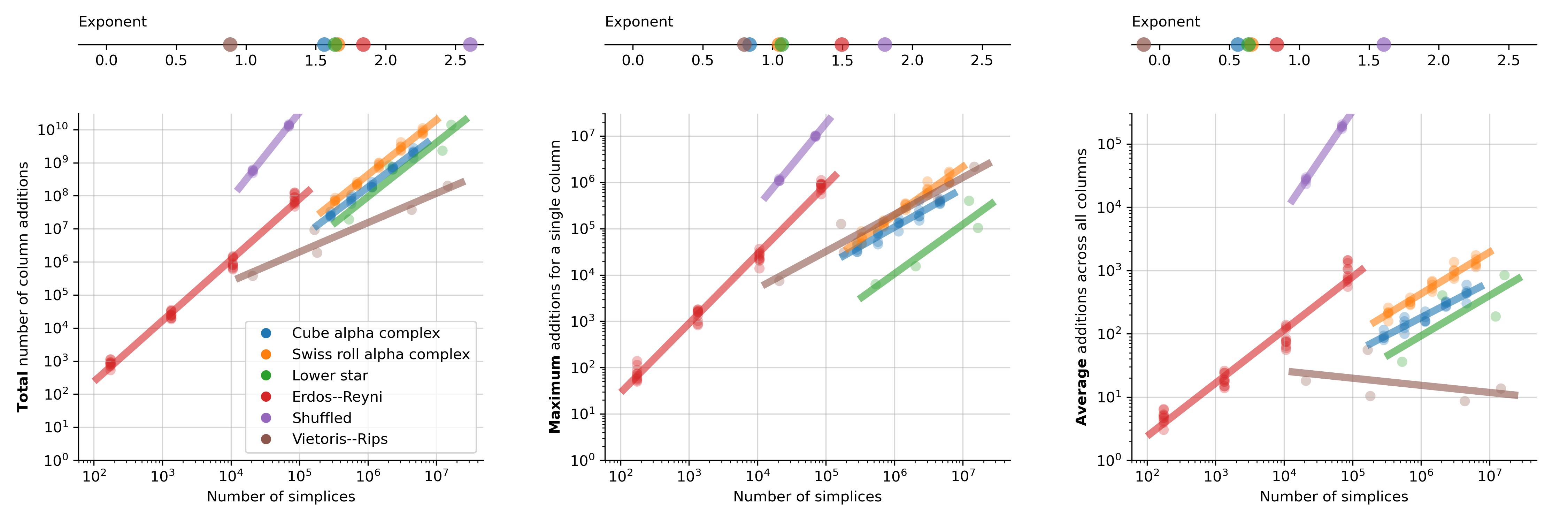
Figure 8: Total number of columns additions (left), maximal number of times a column is used (center), and average number of times a column is used (right) vs number of simplices, for all datasets. In all three plots, the exponent of the log-regression is shown at the top, color-coded.

The leftmost plot shows the total number of column additions, which we use as a proxy of how costly it is to recompute from scratch. Consistently with previous analysis [16, 3], the experimental complexity is much lower than the worst-case complexity (see the exponent at the top). This is especially true for the Vietoris–Rips filtrations, whose total number of columns additions grows sublinearly in the number of simplices. Remarkably, the more random (i.e., less structured) a filtrations is, the faster the number of column operations grows, in accordance with previous evidences.

The plot in the center displays the empirical worst-case: what is the maximal number of additions per column. In other word, how many operations one has to do if they is unlucky and has to remove a heavily used column. Comparing it with the left plot, we see that for almost filtrations the maximum number of column additions grows slower than the total, with the noticeable exception of the Vietoris–Rips filtration. For this latter, the trend is very similar. Nevertheless, for all filtrations, including the Vietoris–Rips, the maximum is at least two order of magnitude smaller than the total number of column operations.

The rightmost plot shows the average number of times each column is used in the reduction, i.e. added to another column. This number is averaged over all the columns and, for the random data, over all iterations with same number of points. The shuffled filtrations is by far the worst-performing, even if this average grows much more slowly than the maximal and the total number of column additions, and it is $2$ order of magnitude smaller than the maximal, and $4$ than then total number of column additions.

The next-worst is the Erdős–Rényi filtration, which is nevertheless growing sublinearly, and whose average number of additions stays at least $2$ order of magnitude below the total number of additions. This is consistent with the findings of [12], where the authors conjecture that the lack of structure of this random filtration is the reason why each column is used almost always to reduce later columns.

The non-random filtration exhibit even more promising trend. The alpha and lower star filtrations behave similarly. In both cases, their average number of addition per column grows sublinearly, and stays between $2$ and $3$ order of magnitude below the maximal number of column additions and $5$ order of magnitude below the total number of column additions. Even more, the average number of additions per column has negative slope for the Vietoris–Rips filtration. This means that the larger the dataset, the smaller the impact of a single column, i.e. the more efficient our method with respect to recomputing the whole filtration. Moreover, the total number of column additions outdistance the average number of additions per column by $4$ order of magnitude on the largest dataset.

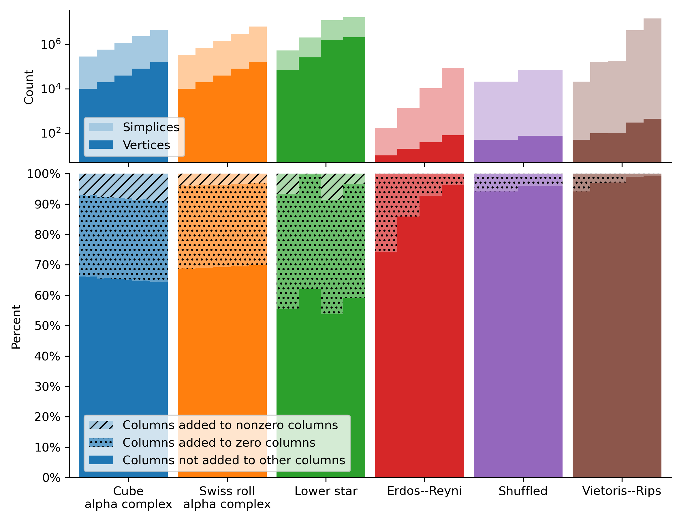
Figure 9: A visual overview of the sizes and column additions necessary when computing persistent homology.

To answer the second question, we display in Figure 9 the percentage of columns that are 1) never used in the reduction (the vast majority of them given by positive simplices), 2) used and added to a zeroed column (and thus can be removed with fewer operations), and 3) used and never added to a zeroed column. As before, for all the randomly sampled inputs we are averaging over the samples.

For all inputs, the majority of columns is not used in the reduction, and therefore their removal require almost no operations. Since Vietoris–Rips, shuffled, and Erdős–Rényi filtrations are full filtrations, none of their columns are maximal simplices (since we capped the degree at $2$) and therefore all satisfy condition in Algorithm 4. Interestingly, the other non-full filtration have a very small percentage of their columns that does not satisfy the condition. Therefore, almost all columns require either none or a small number of operations to be removed. We notice also that only very small percentage of columns is used in the Vietoris–Rips reduction. Combined with the insight from Figure 8, we can conclude that also for the Vietoris–Rips case our method is more efficient than recomputing. A surprising outcome is that the percentage of used columns decreases for increasing number of simplices for the Vietoris-Rips filtration, the Erdős–Rényi filtration, and the shuffled filtration, even if we only have two sizes for the latter, making the analysis less weighty. Therefore, the bigger the dataset the more efficient our methods is compared to recomputing from scratch.

At the top of Figure 9, we displayed the total number of simplices, highlighting how many are vertices. As expected, all clique filtrations have many more higher-dimensional simplices than vertices. In the alpha and lower star filtrations, on the other hand, vertices form the great majority of the total number of simplices. This means that in these filtrations each simplex has few cofaces, which in turn ensure that the for loop in Algorithm 2 is exited quickly.

In conclusion, our experiments show that our method to update the barcode is very likely to be better in practice than recomputing from scratch.

5 Conclusion

We have presented an algorithm to update the barcode of a simplicial complex filtration after a simplex has been removed, demonstrating it to be more efficient than recomputing from scratch. Our work complements existing literature describing rearrangement of and additions to a filtration, completing a full description of how barcode computations can be modified to dynamic changes in the the underlying space.

The next step is to implement our algorithm into some of the most commonly used reduction software [1, 18, 3], and further test its efficiency.

Acknowledgment.

BG was partially or totally supported by the Austrian Science Fund (FWF) grants number P 29984-N35 and P 33765-N. The authors thanks Michael Kerber for useful discussions and support, and David Millman for early exchanges on dynamical zigzags. They also thank Tamal Dey, Michael Kerber, and the anonymous reviews of CompPer 2023 for their feedback on the first version of this work.

References

- [1] Ulrich Bauer. Ripser software. (2016). URL: https://github.com/Ripser/ripser.
- [2] Ulrich Bauer, Michael Kerber, and Jan Reininghaus. Clear and compress: Computing persistent homology in chunks. In Topological Methods in Data Analysis and Visualization III, Theory, Algorithms, and Applications, pages 103–117. Springer, 2014.
- [3] Ulrich Bauer, Michael Kerber, Jan Reininghaus, and Hubert Wagner. PHAT - Persistent Homology Algorithms Toolbox. (2013). URL: https://bitbucket.org/phat-code/phat/src/master/.
- [4] Ulrich Bauer, Talha Bin Masood, Barbara Giunti, Guillaume Houry, Michael Kerber, and Abhishek Rathod. Keeping it sparse: Computing persistent homology revisited, 2022. Preprint available at arXiv:2211.09075.
- [5] Chao Chen and Michael Kerber. Persistent homology computation with a twist. In Proceedings 27th European Workshop on Computational Geometry, 2011.
- [6] David Cohen-Steiner, Herbert Edelsbrunner, and Dmitriy Morozov. Vines and vineyards by updating persistence in linear time. In Proceedings of the Twenty-Second Annual Symposium on Computational Geometry, page 119–126, New York, NY, USA, 2006. Association for Computing Machinery.
- [7] Open Scientific Visualization Datasets. https://klacansky.com/open-scivis-datasets/.
- [8] Tamal K. Dey and Tao Hou. Fast Computation of Zigzag Persistence. In 30th Annual European Symposium on Algorithms (ESA 2022), volume 244 of Leibniz International Proceedings in Informatics (LIPIcs), pages 43:1–43:15, Dagstuhl, Germany, 2022. Schloss Dagstuhl – Leibniz-Zentrum für Informatik.
- [9] Tamal K. Dey and Tao Hou. Updating barcodes and representatives for zigzag persistence, 2022. Preprint available at arXiv:2112.02352.
- [10] Tamal K. Dey and Tao Hou. Computing zigzag vineyard efficiently including expansions and contractions, 2023. Preprint available at arXiv:2307.07462.
- [11] Herbert Edelsbrunner, David Letscher, and Afra Zomorodian. Topological persistence and simplification. In Proceedings 41st annual symposium on foundations of computer science, pages 454–463. IEEE, 2000.
- [12] Barbara Giunti, Guillaume Houry, and Michael Kerber. Average complexity of matrix reduction for clique filtrations. In Proceedings of the 2022 on International Symposium on Symbolic and Algebraic Computation, ISSAC ’22, pages 1–8, New York, NY, USA, 2022. Association for Computing Machinery.
- [13] Barbara Giunti, Jānis Lazovskis, and Bastian Rieck. DONUT: Database of Original & Non-Theoretical Uses of Topology, 2022. https://donut.topology.rocks.
- [14] Woojin Kim, Facundo Mémoli, and Zane Smith. Analysis of dynamic graphs and dynamic metric spaces via zigzag persistence. In Topological Data Analysis, pages 371–389. Springer International Publishing, 2020.
- [15] Yuan Luo and Bradley J. Nelson. Accelerating iterated persistent homology computations with warm starts, 2023. Preprint available at arXiv:2108.05022.
- [16] Nina Otter, Mason A Porter, Ulrike Tillmann, Peter Grindrod, and Heather A Harrington. A roadmap for the computation of persistent homology. EPJ Data Science, 6:1–38, 2017.
- [17] TaDAset - a scikit-tda project. https://github.com/scikit-tda/tadasets, 2018.
- [18] The GUDHI Project. GUDHI User and Reference Manual. GUDHI Editorial Board, 2015. URL: http://gudhi.gforge.inria.fr/doc/latest/.