A Theory of Irrotational Contact Fields

Abstract

We present a framework that enables to write a family of convex approximations of complex contact models. Within this framework, we show that we can incorporate well established and experimentally validated contact models such as the Hunt & Crossley model. Moreover, we show how to incorporate Coulomb’s law and the principle of maximum dissipation using a regularized model of friction. Contrary to common wisdom that favors the use of rigid contact models, our convex formulation is robust and performant even at high stiffness values far beyond that of materials such as steel. Therefore, the same formulation enables the modeling of compliant surfaces such as rubber gripper pads or robot feet as well as hard objects. We characterize and evaluate our approximations in a number of tests cases. We report their properties and highlight limitations.

Finally, we demonstrate robust simulation of robotic tasks at interactive rates, with accurately resolved stiction and contact transitions, as required for meaningful sim-to-real transfer. Our method is implemented in the open source robotics toolkit Drake.

I Introduction

Simulation of multibody systems with frictional contact plays an essential role in robotics. Simulation has been successfully used for hardware optimization, controller design and testing, continuous integration and data generation for machine learning. Moreover, accurate models of physics as used in simulation, enables controller design and model based trajectory optimization algorithms.

However, robust, accurate and performant simulation of multibody systems for contact rich robotics applications remains a formidable challenge.

Rigid body dynamics with frictional contact is complicated by the non-smooth nature of the solutions. Formulated at the acceleration level, rigid contact with Coulomb friction can lead to singular configurations, known as Painlevé paradoxes, for which solutions do not even exist. Discrete formulations at the velocity level circumvent this problem, allowing discrete velocity jumps and impulsive forces. However, discrete formulations introduce an entire family of new problems. Even though many variants exist, in its more general form a discrete formulation enforces balance of momentum subject to contact constraints. Rigid contact is modeled as non-penetration constraints, with additional constraints to enforce Coulomb friction subject to the maximum dissipation principle, introducing new decision variables and Lagrange multipliers. All together, the result is a Non-Linear Complementarity Problem (NCP).

Solving these problems accurately and efficiently however, has remained elusive. This has been explained partly due to the fact that these formulations are equivalent to non-convex problems in global optimization, which are generally NP-hard [1]. An NCP might not admit a solution or, conversely, multiple solutions might exist. A more dangerous outcome in practice is when iterative solvers assume convergence as no additional progress is detected, or resource to early termination to stay within computational budget. These solutions will most often not satisfy the original system of equations and will not obey the laws of physics.

There are other problems that are less talked about — numerical conditioning and implementation details affect convergence properties and robustness. These are important problems when it comes to simulation of complex systems, with either a large number of degrees of freedom (DOFs), large number of constraints or both. Solutions that work for small systems, often do not work when faced with real life engineering applications.

In an attempt to make the problem tractable, Anitescu introduced a convex approximation of contact [2]. This work effectively replaces the original NCP by a convex approximation with existence guarantees. Later, Todorov [3] regularizes this formulation to write a strictly convex formulation with a unique solution. Our previous work [4] introduces the convex Semi-Analytic Primal (SAP) formulation for the modeling of compliant contact. SAP embraces compliance to provide a robust and performant tool that targets robotics applications — grippers have compliant surfaces to establish stable grasps, and robotic feet are most often padded with compliant surfaces. Although the formulation is inherently compliant, rigid contact can be modeled to good approximation using a near-rigid approximation. The work focuses on physical correctness, numerical conditioning and robustness.

However, the SAP formulation has a number of limitations. The most well known is the artifact of gliding during slip, an artifact inherited from the original formulation by Anitescu [5] and shared with Todorov’s formulation [3] as well. As objects slip, they glide at a finite distance $\delta t\mu\|{\bm{v}}_{t}\|$, proportional to the time step $\delta t$, coefficient of friction $\mu$ and slip velocity $\|{\bm{v}}_{t}\|$. While the artifact vanishes in the limit to zero time step size, the effect can be significant at the large time step sizes required for interactive simulations. Moreover, in this work we show that SAP’s compliant model as well as Todorov’s regularized model, are inconsistent — the gliding effect does not vanish as time step goes to zero. This is not only nonphysical but also makes the selection of modeling parameters cumbersome for the user, having to select dissipation parameters appropriate for their application, but still low enough so that the gliding artifact is not largely pronounced. Finally, SAP’s model of compliance is intrinsic to its convex formulation, and therefore it is not possible to incorporate other well known and experimentally validated models of contact, such as Hertz and Hunt & Crossley [6].

Still, the SAP formulation leads to a robust solution, with theoretical convergence guarantees that transfer to a practical software implementation. Therefore, the objective of this work is to extend the SAP formulation to reduce and even eliminate many of these limitations while still preserving SAP’s convexity along with convergence and robustnees guarantees.

II Novel Contributions

The present work aims to extend the convex SAP formulation [4] for the modeling of compliant contact. This extension seeks to mitigate nonphysical artifacts introduced by the convex approximation, to incorporate experimentally validated models of contact, to increase the fidelity of frictional contact, and to improve numerics.

Our contribution not only extends our previous SAP work, but also builds upon previous research on incremental potentials [7]. Previous work implements Incremental Potential Contact (IPC) [8] for a method that guarantees intersection free solutions. The authors demonstrate their method in a large variety of simulation cases. Being non-convex however, as with NCPs, the formulation can either have no solution (the feasible set is empty) or fall into a local minimum that does not obey physics.

Therefore, the focus of this work is to develop conditions for convexity to design incremental potentials that can be immediately incorporated into our convex SAP [9] formulation. To the knowledge of the authors, conditions for convexity have never been explored.

We summarize our contributions as follows

1. We introduce a framework that allows to incorporate contact models with arbitrary functional form, and establish conditions for convexity.

2. We develop the necessary conditions a contact model must satisfy in order for a in incremental potential to exist. Moreover, we provide additional conditions for convexity.

3. We introduce a framework for regularized friction that allows to incorporate Coulomb friction given an arbitrary model of normal forces. The framework incorporates arbitrary forms of regularization, allowing to design accurate models with desired numerical properties.

4. We use this new framework to develop a convex approximation to a model of compliant contact with Hunt & Crossly dissipation [6].

5. We show the same framework can be used to incorporate barrier functions to model rigid contact. However, after numerical experimentation that shows our solution is robust even at stiffness values as high as that of steel, this work favors compliant models.

6. In addition to SAP, we develop two new formulations of contact with dry friction within this same framework.

In addition to these main research contributions, our work includes an open source implementation in Drake [10]. We compare models in Section VII, validate them in Section IX and stress test them with engineering applications cases in Section X.

III Mathematical Formulation

We first introduce notation and conventions used in our framework. We closely follow the notation in our previous work [4, 11] later extended to deformable FEM models in [12].

The state of our system is described by generalized positions ${\mathbf{q}}\in\mathbb{R}^{n_{q}}$ and generalized velocities ${\mathbf{v}}\in\mathbb{R}^{n_{v}}$ where $n_{q}$ and $n_{v}$ denote the total number of generalized positions and velocities, respectively. Time derivatives of the configurations relate to the generalized velocities by the kinematic map $\dot{{\mathbf{q}}}={\mathbf{N}}({\mathbf{q}}){\mathbf{v}}$. We use joint coordinates to describe articulated rigid bodies.

Consider a system with $n_{c}$ constraints. Constraint velocities are given by ${\mathbf{v}}_{c}={\mathbf{J}}{\mathbf{v}}+{\mathbf{b}}$, where ${\mathbf{J}}$ is the stacked Jacobian for all constraints and ${\mathbf{b}}$ is a bias term. The SAP formulation in our previous work [4], writes a linearized balance of momentum equation as

$${\mathbf{A}}({\mathbf{v}}-{\mathbf{v}}^{*})={\mathbf{J}}^{T}{\bm{\gamma}},$$ (1)

where ${\mathbf{v}}^{*}$ are the free motion velocities when contact impulses are zero, ${\bm{\gamma}}$ are the constraint impulses and ${\mathbf{A}}$ is the gradient of the discrete inverse dynamics. Early work uses ${\mathbf{A}}={\mathbf{M}}({\mathbf{q}}_{0})$, the mass matrix at the previous time step [13, 14]. The SAP formulation is simply extending this idea to incorporate, for instance, the modeling of joint springs, damping and rotor inertia implicitly. Refer to [4] for details. Traditional NCP formulations supplement (1) with constraint equations to model contact. Additional constraint equations, slack variables and Lagrange multipliers lead to a large and challenging to solve NCP.

SAP [4] follows a different approach. Inspired by the analytical inverse dynamics from Todorov [3], SAP eliminates constraints analytically to write an unconstrained convex optimization problem for the next time step velocities

$$\min_{{\mathbf{v}}}\ell_{p}({\mathbf{v}})=\frac{1}{2}\|{\mathbf{v}}-{\mathbf{v}}^{*}\|_{A}^{2}+\ell_{R}({\mathbf{v}}),$$ (2)

where $\|{\mathbf{x}}\|_{A}^{2}={\mathbf{x}}^{T}{\mathbf{A}}\,{\mathbf{x}}$, and $\ell_{R}({\mathbf{v}})$ is a regularizing term that penalizes contact impulses. It can be shown that SAP’s [4] formulation models compliant contact with a linear spring law and a linear model of damping. A follow-up work [11] shows how to include the modeling of continuous contact surfaces in this framework. The formulation is strongly convex, with strong convergence guarantees that transfer to practical software implementations. Although the formulation is inherently compliant with regularized friction, [4] shows how rigid contact can be modeled to good approximation using a near-rigid approximation.

Inspired by [8] on incremental potentials, we extend this formulation by replacing the regularizer cost $\ell_{R}({\mathbf{v}})$ by a more general cost or incremental potential $\ell_{c}({\mathbf{v}};{\mathbf{x}}_{0})$ to model contact and other constraints. In this notation, this potential is a function of the generalized velocities ${\mathbf{v}}$, given a previous state ${\mathbf{x}}_{0}$ of the system. This makes these potentials inherently discrete, unlike physical potentials such as the gravity and electric fields, which are only a function of the current (continuous) configuration of the system. We’ll see however how these discrete incremental potentials relate to physics in the following sections. Given the presence of the quadratic term $\|{\mathbf{x}}\|_{A}^{2}$, the total optimization problem (2) is strongly convex for as long as $\ell_{c}$ is convex, and its solution exists and is unique. However, convex potentials for the modeling of frictional contact are not trivial to construct and are thus the main topic of this work.

Within this framework, the balance of momentum (1) is the optimality condition of (2), and impulses emerge as a result of the contact potentials

$${\bm{\gamma}}({\mathbf{v}}_{c};{\mathbf{x}}_{0})=-\frac{\partial\ell_{c}({\mathbf{v}}_{c};{\mathbf{x}}_{0})}{\partial{\mathbf{v}}_{c}}.$$ (3)

As with the SAP formulation, we consider potential functions that are separable

$$\ell_{c}({\mathbf{v}}_{c};{\mathbf{x}}_{0})=\sum_{i=1}^{n_{c}}\ell_{c,i}({\bm{v}}_{c,i};{\mathbf{x}}_{0}),$$ (4)

where ${\mathbf{v}}_{c}$ is the stacked vector of individual constraint velocities ${\bm{v}}_{c,i}$. For contact constraints, we define a contact frame $C_{i}$ for which we arbitrarily choose the $z\text{-axis}$ to coincide with the contact normal $\hat{{\bm{n}}}_{i}$. In this frame the normal and tangential components of ${\bm{v}}_{c,i}$ are given by $v_{n,i}=\hat{{\bm{n}}}_{i}\cdot{\bm{v}}_{c,i}$ and ${\bm{v}}_{t,i}={\bm{v}}_{c,i}-v_{n,i}\hat{{\bm{n}}}_{i}$ respectively, so that ${\bm{v}}_{c,i}=[{\bm{v}}_{t,i}\,v_{n,i}]$. By convetion, we define the relative contact velocity ${\bm{v}}_{c,i}$ and normal $\hat{{\bm{n}}}_{i}$ such that $v_{n,i}>0$ for objects moving away from each other.

Using this separable potential (4) in (3), we see that the impulse vector ${\bm{\gamma}}$ is the stacked vector of individual constraint contributions ${\bm{\gamma}}_{i}({\mathbf{v}}_{c,i};{\mathbf{x}}_{0})=-\partial\ell_{c,i}/\partial{\mathbf{v}}_{c,i}$. Notice we dragged the dependence on the previous time step state ${\mathbf{x}}_{0}$ along to emphasize the discrete (or incremental) nature of these potentials and the resulting impulses. However, hereinafter we write ${\bm{\gamma}}_{i}({\bm{v}}_{c,i})$ and $\ell_{c,i}({\bm{v}}_{c,i})$ to shorten notation, and the functional dependence on the previous time step state is assumed implicit.

In the next sections we derive these potentials for the modeling of frictional contact.

IV Frictionless Contact

We first consider the frictionless case, allowing us to introduce the mechanics of the framework and additional notation.

We consider a generic functional form for the normal force

$$f_{n}(x,\dot{x}),$$ (5)

as a function of the penetration distance $x$ (defined positive when objects overlap) and its rate of change $\dot{x}$. To write a discrete incremental potential, we use a first order approximation of the penetration distance $x=x_{0}+\delta t\dot{x}$, implicit on the next time step rate $\dot{x}$. Given our sign convention for $v_{n}$ (positive when objects separate), we note that $\dot{x}=-v_{n}$. Using this approximation, we define a discrete impulse as

$$n(v_{n};x_{0})=\delta t\,f_{n}(x_{0}-\delta t\,v_{n},-v_{n}),$$ (6)

and the normal impulse is $\gamma_{n}(v_{n})=n(v_{n};x_{0})$. Therefore, the potential for such model is given by

$$\ell_{n}(v_{n})=-N(v_{n}),$$ (7)

where $N(v_{n})$ is the antiderivative of $n(v_{n})$, i.e. $n(v_{n})=N^{\prime}(v_{n})$.

The Hessian of this cost is

$$\frac{d^{2}\ell_{n}}{dv_{n}^{2}}=\delta t^{2}\frac{\partial f_{n}}{\partial x}+\delta t\frac{\partial f_{n}}{\partial\dot{x}},$$ (8)

and therefore $\partial f_{n}/\partial x\geq 0$ and $\partial f_{n}/\partial\dot{x}\geq 0$ imply that the cost $\ell_{n}(v_{n})$ is convex.

IV-A Barrier Functions for Rigid Contact

Interior-point methods (IP) have become a gold standard for the solution of optimization problems with inequality constraints, as required for the modeling of rigid contact. These methods were able to exploit advances in computer architecture, including the introduction of multi-core processors and SIMD instruction sets. Moreover, solvers in this family can incorporate a richer set of constraints such as conic constraints, as needed for the modeling of Coulomb friction. Popular open source software includes Ipopt [15], while proprietary implementations include Gurobi and Mosek. While variants exist, at its core, this method replaces constraints with a barrier function that penalizes unfeasible solutions. Logarithmic functions are standard, which for rigid contact penalizes negative penetrations

$$\ell_{n}(x)=-\kappa\ln(-x),$$ (9)

while penetration states ($x>0$) are unfeasible. The barrier parameter $\kappa>0$ is iteratively reduced to approach the rigid solution, though it can never reach zero. Therefore, in the practical limit of numerical solvers, the solution is effectively compliant, with a force law that fits the framework (5)

$$f_{n}(x,\dot{x})=-\frac{\kappa}{x}\quad\forall x<0.$$ (10)

As a physical model of contact, users would have a hard time making sense of (10), with a parameter $\kappa$ with units of energy and nonphysical action at infinite distance (even if negligible). In practice, $\kappa$ is not exposed, but hidden as part of the solver internals. The user believes in a true model of rigid contact when in reality a compliant model is used by the solver. Even if $\kappa$ can be brought to very small values (in some metric, also hidden to users), most likely the solver is solving a much more challenging problem than needed, since in reality physical materials have finite stiffness.

IV-B Incremental Potential Contact

The IPC method [8] is an optimization based framework developed to model rigid contact robustly and obtain intersection free solutions. The method attains good robustness given its implicit time-stepping scheme, similar to ours. The key difference however, is that IPC formulates a non-convex optimization problem. Being non-convex, the solver can fall into local minima, not satisfying the original physics. Moreover, IPC lags normal forces at each iteration (effectively a fixed iteration), an approach with no convergence guarantees, as properly pointed out by the original authors. The authors augment their line search with continuous collision detection (CCD) to maintain feasibility.

Similar to the logarithmic barrier functions of IP methods, IPC proposes a smooth $C^{2}$ potential

$$\ell_{c}(x)=-\kappa_{\text{IPC}}\,(x+\hat{d})_{+}^{2}\ln(-x/\hat{d})$$ (11)

where $(a)_{+}=\max(0,a)$, $\kappa_{\text{IPC}}$ is a barrier parameter adjusted automatically to improve numerical conditioning and $\hat{d}$ is a parameter set by the user. Unlike the traditional barrier function, this potential is zero when objects are farther than a distance $\hat{d}$. This potential is proposed to achieve intersection free solutions and eliminate action at infinite distances, while maintaining smoothness for better performance of the Newton iterations used by the solver. We see however, that this method once again fits the framework (5), with a compliant contact force law of the form

$$f_{n}(x,\dot{x})=\kappa_{\text{IPC}}\,(x+\hat{d})_{+}\left[\frac{(x+\hat{d})_{+}}{x}-2\ln(-x/\hat{d})\right],$$ (12)

which is only non-zero when $-\hat{d}<x<0$.

Typical values of $\hat{d}$ used by the original authors in their extensive set of simulations cases is in the range $0.1\text{ mm}$ to $1\text{ mm}$. That is, this method models a thin compliant layer around a solid core, rather than the strict non-penetration conditions largely favored in the literature.

We do not see this as a flaw, given the authors demonstrate the effectiveness of their method with extensive simulation studies, but rather as an indication of the levels of rigidity attainable in practice.

IV-C Compliant Contact

In previous sections we show that even solvers for rigid contact are effectively compliant when we analyze them in detail. That’s precisely why in this work we embrace compliance to write a model that is transparent to users, with physics based parameters.

Here we consider a linear elastic law in the penetration distance $x$ with a Hunt & Crossley [6] model of dissipation. Other alternatives, for instance based on Hertz theory can be included within the same framework. In practice however, we found that users find the linear spring model appropriate for their applications when using point contact. Moreover, this model can be extended to model continuous contact patches with no changes to the solver [11].

We write this contact law within framework (5) as

$$f_{n}(x,\dot{x})=k\,x_{+}\,(1+d\dot{x})_{+},$$ (13)

where where $k$ is the linear contact stiffness and $d$ is the Hunt & Crossley dissipation parameter.

We see from (13) that the force is zero whenever $v_{n}\geq\hat{v}$, with $\hat{v}=\min(x_{0}/\delta t,1/d)$. Then for $v_{n}<\hat{v}$ we define the (indefinite) antiderivative $N^{+}(v_{n})$ for when $n(v_{n})>0$

$$N^{+}(v_{n};x_{0}) =$$ (14)

$$\delta t\,k\,\left[v_{n}\left(x_{0}-\frac{1}{2}\delta t\,v_{n}\right)-d\,\frac{v_{n}^{2}}{2}\left(x_{0}-\frac{2}{3}\delta t\,v_{n}\right)\right],$$

However, we define the elastic contribution at the previous time step $f_{0}=k\,x_{0}$ and write instead

$$N^{+}(v_{n};f_{0}) =$$ (15)

$$\delta t\left[v_{n}\left(f_{0}+\frac{1}{2}\Delta f\right)-d\,\frac{v_{n}^{2}}{2}\left(f_{0}+\frac{2}{3}\Delta f\right)\right],$$

with $\Delta f=-\delta t\,k\,v_{n}$. This form is numerically more stable to incorporate the modeling of continuous contact patches [11] for which it is possible to have $k=0$ (or close to zero) for small face patches, but with a finite value of the product $f_{0}=k\,x_{0}$. We observe that this potential is cubic in $v_{n}$ for $d>0$, in contrast to the quadratic SAP potential for linear dissipation.

Since the impulse is zero for $v_{n}\geq\hat{v}$, its antiderivative must be constant. Therefore, we write

$$N(v_{n})=N^{+}(\min(v_{n},\hat{v});f_{0}),$$ (16)

resulting in a continuous function for all values of $v_{n}$.

We observe that even though this model is compliant, we can model very stiff contact given the robustness of our convex formulation. For instance, in Sections IX, we use Hertz theory to estimate a linear stiffness $k=10^{7}\text{ N}/\text{m}$ for steel. Even though larger values are simply nonphysical, we show in Section X that our formulation can robustly handle stiffness values five orders of magnitude larger. Moreover, stiffness values two orders of magnitude smaller, are still suitable for the approximation of rigid contact.

V Contact with Friction

V-A Regularized Friction

As with normal contact impulses $\gamma_{n}(v_{n})$, friction impulses can also be modeled as a continuous function of state using a regularized approximation. Consider the following model of isotropic friction

$${\bm{\gamma}}_{t}({\bm{v}}_{c}) = -\mu\,f(\|{\bm{v}}_{t}\|/\varepsilon_{s})\,\gamma_{n}(v_{n})\,\hat{{\bm{t}}}$$

$$f(s) = \frac{s}{\sqrt{1+s^{2}}}$$ (17)

$$\hat{{\bm{t}}} = \frac{{\bm{v}}_{t}}{\|{\bm{v}}_{t}\|}$$

where the function $f(s)\leq 1$ regularizes Coulomb friction with $\varepsilon_{s}$ the regularization parameter. For $\|{\bm{v}}_{t}\|\ll\varepsilon_{s}$ the model behaves as viscous damping with high viscosity. For $\|{\bm{v}}_{t}\|\gg\varepsilon_{s}$ the model approximates Coulomb’s law, with friction opposing slip velocity according to the maximum dissipation principle and $\|{\bm{\gamma}}_{t}\|=\mu\gamma_{n}$. The choice of function $f(s)$ is somewhat arbitrary for as long as $f(s)\leq 1$ and $f(s)=0$ at $s=0$. In particular, we choose the functional form of $f(s)$ in (17) because, when expanded, (17) can be simplified to

$${\bm{\gamma}}_{t}({\bm{v}}_{c}) = -\mu\,\gamma_{n}(v_{n})\,\hat{{\bm{t}}}_{s}$$

$$\hat{{\bm{t}}}_{s} = \frac{{\bm{v}}_{t}}{\sqrt{\|{\bm{v}}_{t}\|^{2}+\varepsilon_{s}^{2}}}$$ (18)

where we defined the regularized or soft tangent vector $\hat{{\bm{t}}}_{s}$ which can be shown to be the gradient with respect to ${\bm{v}}_{t}$ of the soft norm $\|{\bm{x}}\|_{s}=\sqrt{\|{\bm{x}}\|^{2}+\varepsilon_{s}^{2}}-\varepsilon_{s}$, see Appendix A. Unlike $\hat{{\bm{t}}}$, which is not even well-defined at ${\bm{v}}_{t}={\bm{0}}$, $\hat{{\bm{t}}}_{s}$ is well-defined and continuous for all values of slip velocity. Moreover, not only (18) is continuous but also its gradients with respect to ${\bm{v}}_{t}$. We’ll find this later to be a very desired property so that the Hessian of our convex formulation is continuously well-behaved, improving the convergence rate of Newton iterations.

At this point however, it is not even clear if possible to incorporate such a model of frictional contact into a convex formulation. We do know SAP [4] to be a convex formulation of regularization friction, though with a form different from (17)

$${\bm{\gamma}}_{t}({\bm{v}}_{c}) = -\min\left(\frac{\|{\bm{v}}_{t}\|}{R_{t}},\mu\gamma_{n}(v_{n})\right)\hat{{\bm{t}}}$$ (19)

where $R_{t}$ is SAP’s regularization parameter [4]. In the following sections we investigate the conditions to write convex approximations for models in the form of (17). We seek for a superior model to SAP’s for two reasons

1. SAP’s linear model of dissipation can lead to severe artifacts at large dissipation values, see Section IX. Therefore, we seek to incorporate more complex models such as the experimentally validated Hunt & Crossley model.

2. SAP’s regularization and it’s connection to drift during stiction is well studied and characterized in [4]. Though bounds to the drift speed can be estimated, it is not possible to determine it precisely. In contrast, drift for the model (17) is well determined by parameter $\varepsilon_{s}$.

V-B Existence of a Potential. Irrotational Fields

We can combine the models of compliant contact with regularized friction from previous sections to write

$${\bm{\gamma}}({\bm{v}}_{c}) = \begin{bmatrix}-\mu\,n(v_{n})\,\hat{{\bm{t}}}_{s}({\bm{v}}_{t})\\ n(v_{n})\end{bmatrix}.$$ (20)

This is done for instance in [9]. However, this model is not the result of potential and ${\bm{\gamma}}({\bm{v}}_{c})\neq-\partial\ell_{c}/\partial{\bm{v}}_{c}$. In this section we seek to establish the conditions for a (possibly convex) potential $\ell_{c}({\mathbf{v}})$ to exist. Additional conditions for convexity are established separately.

Helmholtz’s theorem tells us that any vector field admits the decomposition into an irrotational field (zero curl) and a solenoidal field (zero divergence)

$${\bm{\gamma}}({\bm{v}}_{c})=-\nabla\ell({\bm{v}}_{c})+\nabla\times{\bm{A}}({\bm{v}}_{c})$$ (21)

where $\ell({\bm{v}}_{c})$ is a scalar potential and ${\bm{A}}({\bm{v}}_{c})$ is referred to as the vector potential. Therefore, we cannot expect in general that any contact model (20) can be expressed as the gradient of a scalar potential. We can however investigate what kind of approximations we can obtain by ignoring the solenoidal component of the field.

We can write a PDE for the scalar potential if we take the divergence of (21)

$$\nabla^{2}\ell=-\nabla\cdot{\bm{\gamma}}$$ (22)

and therefore for a known divergence $\nabla\cdot{\bm{\gamma}}$, and suitable boundary conditions, we can find the potential by solving this equation. Coming up with appropriate boundary conditions to model frictional contact is not trivial and, in particular, it has not obvious physical significance. Instead, we investigate the conditions that the resulting impulses must satisfy for the potential to exist.

From Eq. (21), if such a potential exists, then the impulse function or field ${\bm{\gamma}}({\bm{v}}_{c})$ must be irrotational, and its curl is zero. That is

$$\nabla\times{\bm{\gamma}}={\mathbf{0}}$$ (23)

The normal component in (23) leads to the condition

$$\frac{\partial\gamma_{t,1}}{\partial v_{t,2}}=\frac{\partial\gamma_{t,2}}{\partial v_{t,1}}$$ (24)

which simply states that the two-dimensional tangential field ${\bm{\gamma}}_{t}({\bm{v}}_{t})$ is irrotational in the ${\bm{v}}_{t}$ plane.

We can see that isotropic friction fields are irrotational. Consider the generic functional form for an isotropic friction model

$${\bm{\gamma}}_{t}=g(\|{\mathbf{v}}_{t}\|,v_{n})\hat{{\mathbf{t}}}$$ (25)

whose gradient is

$$\frac{\partial{\bm{\gamma}}_{t}}{\partial{\mathbf{v}}_{t}}=\frac{\partial g}{\partial\|{\mathbf{v}}_{t}\|}{\mathbf{P}}+g\frac{{\mathbf{P}}^{\perp}}{\|{\mathbf{v}}_{t}\|}$$ (26)

with symmetric projection matrices ${\mathbf{P}}$ and ${\mathbf{P}}^{\perp}$ as defined in Appendix A. Therefore, $\partial{\bm{\gamma}}_{t}/\partial{\mathbf{v}}_{t}$ is symmetric and therefore condition (24) is met. Vector fields from anisotropic friction models are generally not irrotational. The friction force is no longer antiparallel to the slip velocity, and objects follow curved paths [16]. Therefore, from now on, we focus on isotropic friction models in the form (25).

Finally, the tangential components in (23) lead to the condition

$$\frac{\partial{\bm{\gamma}}_{t}}{\partial v_{n}}=\frac{\partial\gamma_{n}}{\partial{\mathbf{v}}_{t}}$$ (27)

and it is not trivially met in general by arbitrary contact models.

VI A Family of Contact Models

In this section we find a family of contact models that satisfy condition (27), and thus can be written as the gradient of a potential function. In addition, we establish additional conditions for convexity.

VI-A SAP model

While SAP [4] is convex by construction, it is a good exercise to verify our newly developed conditions hold for this model. From [4] we know that the Hessian of the regularizer cost

$${\mathbf{G}}=\frac{\partial^{2}\ell}{\partial{\mathbf{v}}_{c}^{2}}=-\frac{\partial{\bm{\gamma}}}{\partial{\mathbf{v}}_{c}}=-\begin{bmatrix}\frac{\partial{\bm{\gamma}}_{t}}{\partial{\mathbf{v}}_{t}}&\frac{\partial{\bm{\gamma}}_{t}}{\partial v_{n}}\\ \frac{\partial\gamma_{n}}{\partial{\mathbf{v}}_{t}}^{T}&\frac{\partial\gamma_{n}}{\partial v_{n}}\\ \end{bmatrix}$$ (28)

is symmetric positive semi-definite and therefore SAP meets the condition in (27), as expected. Moreover $\partial{\bm{\gamma}}_{t}/\partial{\mathbf{v}}_{t}$ is symmetric since ${\bm{\gamma}}_{t}$ is of the isotropic form (25) and condition (24) is met.

VI-B Lagged Model

We use the model of regularized friction (17) in which the normal impulse is lagged to the previous time step

$${\bm{\gamma}}_{t}({\bm{v}}_{t})=-\mu\,f(s)\gamma_{n,0}\hat{{\mathbf{t}}}$$ (29)

with $s=\|{\mathbf{v}}_{t}\|/\varepsilon_{s}$, and where using (5), $\gamma_{n,0}=\delta tf_{n}(x_{0},\dot{x}_{0})$. For a physical model of compliance for which $\gamma_{n}$ is only a function of $v_{n}$, condition (27) is trivially met since

$$\frac{\partial{\bm{\gamma}}_{t}}{\partial v_{n}}={\mathbf{0}}$$

$$\frac{\partial\gamma_{n}}{\partial{\mathbf{v}}_{t}}={\mathbf{0}}$$

In this model, the normal impulses are still treated implicitly, with potential $\ell_{n}=-N(v_{n})$ and impulse $\gamma_{n}=n(v_{n})$. The normal impulse is only lagged in the friction model.

We can verify that

$$\ell_{t}({\bm{v}}_{t})=\mu\gamma_{n0}\,\varepsilon_{s}\,F(\|{\bm{v}}_{t}\|/\varepsilon_{s})$$ (30)

with $f=F^{\prime}$ satisfies ${\bm{\gamma}}_{t}=-\partial\ell_{t}/\partial{\mathbf{v}}_{t}$ and therefore $\ell_{t}({\bm{v}}_{t})$ is the corresponding potential function.

For this lagged model the total potential is separable in normal and friction contributions

$$\ell({\bm{v}}_{c})=\ell_{t}({\bm{v}}_{t})+\ell_{n}(v_{n})$$ (31)

The Hessian for $\ell_{t}$ is given by

$$\frac{\partial^{2}\ell_{t}}{\partial{\bm{v}}_{t}^{2}} = -\frac{\partial{\bm{\gamma}}_{t}}{\partial{\bm{v}}_{t}}$$ (32)

$$= \mu\gamma_{n0}\left[\frac{f^{\prime}(s)}{\varepsilon_{s}}{\mathbf{P}}(\hat{{\bm{t}}})+\frac{f(s)}{\|{\bm{v}}_{t}\|}{\mathbf{P}}^{\perp}(\hat{{\bm{t}}})\right]$$

With $f$ non-decreasing, $F$ is convex, and the Hessian of $\ell_{t}$ is the positive linear combination of two projection matrices. Therefore, $\ell_{t}$ is twice differentiable and convex.

As pointed out in Section V-A, unit vector $\hat{{\bm{t}}}$ is not well-defined at ${\bm{v}}_{t}={\bm{0}}$ and both gradient and Hessian of $\ell_{t}$ are singular. We can remove this singularity with a judicious choice of the function $F(s)$. Choosing $F(s)=\sqrt{s^{2}+1}-1$ leads to expressions of the cost, gradient and Hessian involving soft norms (Appendix A) which are twice differentiable and convex, even at ${\bm{v}}_{t}={\bm{0}}$

$$\ell_{t}({\bm{v}}_{t}) =\mu\gamma_{n0}\,\|{\bm{v}}_{t}\|_{s},$$

$${\bm{\gamma}}_{t} =-\mu\,\gamma_{n,0}\hat{{\mathbf{t}}}_{s},$$

$$\frac{\partial^{2}\ell_{t}}{\partial{\bm{v}}_{t}^{2}} =\mu\gamma_{n0}\frac{{\mathbf{P}}^{\perp}(\hat{{\bm{t}}}_{s})}{\|{\bm{v}}_{t}\|_{s}+\varepsilon_{s}}$$ (33)

VI-C Similar Model

Similarity solutions to PDEs are solutions which depend on certain groupings of independent variables, rather than on each variable separately. In particular, self-similar solutions arise when the problem lacks a characteristic time or length scale. The Blasius solution to Prandtl’s boundary layer equations in fluid mechanics is a well-known celebrated example.

SAP [4], as well as previous work on convex approximations of contact [2, 3], introduce an artifact in which objects glide at a distance $\delta t\mu\|{\bm{v}}_{t}\|$ only when sliding. This effect vanishes as time step size goes to zero. Motivated by the algebraic form of SAP impulses with formula provided in [4], we propose the grouping of variables $z=v_{n}-\mu\|{\bm{v}}_{t}\|$. Furthermore, we generalize this grouping to

$$z=v_{n}-\mu\varepsilon_{s}F(s),$$ (34)

where, using notation from Section VI-B, the term $\mu\varepsilon_{s}F(s)$ simplifies to $\mu\|{\bm{v}}_{t}\|_{s}$ when $F(s)=\sqrt{s^{2}+1}-1$. Note the consistency of units in (34), an inportant aspect of similar solutions. With this grouping, we propose the similar solution

$$\gamma_{n}(\|{\bm{v}}_{t}\|,v_{n}) = n(z),$$

$${\bm{\gamma}}_{t}(\|{\bm{v}}_{t}\|,v_{n}) = -\mu\,f(s)\,\gamma_{n}(\|{\bm{v}}_{t}\|,v_{n})\,\hat{{\bm{t}}}$$ (35)

We observe that, unlike the lagged model, this similar model strongly couples the friction and normal components. This however comes at the cost of a model in which the normal component depends on the slip velocity, an artifact of the approximation. We characterize the strength of this artifact in the following sections.

Direct differentiation of (35) leads to

$$\frac{\partial{\bm{\gamma}}_{t}}{\partial v_{n}}=\frac{\partial\gamma_{n}}{\partial{\mathbf{v}}_{t}}=-\mu\,f(s)\,n^{\prime}(z)\,\hat{{\bm{t}}}$$

which confirm condition (27) is satisfied. Therefore, there exists a potential $\ell$ such that ${\bm{\gamma}}=\partial\ell/\partial{\bm{v}}_{c}$.

We start from the normal component of the impulse

$$\gamma_{n}(\|{\bm{v}}_{t}\|,v_{n})=n(z)=-\frac{\partial\ell}{\partial v_{n}},$$ (36)

and integrate it on $v_{n}$ to obtain

$$\ell({\bm{v}}_{t},v_{n})=-N(z)+G({\bm{v}}_{t}),$$ (37)

where $G({\bm{v}}_{t})$ is an arbitrary function of ${\bm{v}}_{t}$. Taking the derivative with respect to ${\bm{v}}_{t}$ results in

$$\frac{\partial\ell}{\partial{\bm{v}}_{t}}=\mu\,n(z)\,f(s)\hat{{\bm{t}}}+\frac{\partial G}{\partial{\bm{v}}_{t}}.$$ (38)

Comparing this last equation with (35) reveals we can take $G=0$ and therefore

$$\ell(\|{\bm{v}}_{t}\|,v_{n})=-N(z),$$ (39)

is the desired potential function.

The Hessian of this potential is

$$\frac{\partial^{2}\ell}{\partial{\bm{v}}_{c}^{2}}=-\frac{\partial{\bm{\gamma}}}{\partial{\bm{v}}_{c}}=$$ (40)

$$\begin{split}=&\mu\left[\left(\frac{f^{\prime}(s)n(z)}{\varepsilon_{s}}-n^{\prime}(z)f^{2}(s)\right){\mathbf{P}}(\hat{{\bm{t}}})\right.\\ &+\left.\frac{f(s)n(z)}{\|{\bm{v}}_{t}\|}{\mathbf{P}}^{\perp}(\hat{{\bm{t}}})\right].\end{split}$$

For a convex potential $\ell_{n}$ we have $n^{\prime}=N^{\prime\prime}=-\ell_{n}^{\prime\prime}\leq 0$. With $f(s)$ non-decreasing as in the lagged model, $f^{\prime}\geq 0$. Then the Hessian $\partial^{2}\ell/\partial{\bm{v}}_{c}^{2}$ is the linear combination with positive coefficients of symmetric positive semi-definite projection matrices. Therefore the Hessian is symmetric positive semi-definite and the potential is convex.

As before, a judicious choice of $f(s)$ leads to continuous gradient and Hessian. Once again we take $F(s)=\sqrt{s^{2}+1}-1$, leading to expressions in which the soft norm $\|{\bm{v}}_{t}\|_{s}$ (Appendix A) replaces $\|{\bm{v}}_{t}\|$ and $\hat{{\bm{t}}}_{s}$ replaces $\hat{{\bm{t}}}$, removing the singularity at ${\bm{v}}_{t}={\bm{0}}$.

VII Comparative Analysis of the Models

All the models presented in Section VI are convex approximations of contact, each with its own strengths and limitations. Hereinafter we refer to each of these formulations to as SAP [4], Lagged (section VI-B), and Similar (section VI-C). We summarize their properties in Table I and expand in the following subsections.

Model	Consistent	Strongly coupled	Gliding during slip	Compliance modulation		Transition slip
				Stiffness	Dissipation
SAP	No	Yes	$\mu(\delta t+\tau_{d})\|{\bm{v}}_{t}\|$	$k/(1+\tilde{\mu}^{2})$	$\tau_{d}$	$\sigma\,\text{w}\,\mu\,\gamma_{n}$
Lagged	Yes	No	—	$k$	$d$	$v_{s}$
Similar	No	Yes	$\mu\delta t\|{\bm{v}}_{t}\|$	$k\,(1+\mu\,d\,\|{\bm{v}}_{t}\|)$	$d/(1+\mu\,d\,\|{\bm{v}}_{t}\|)$	$v_{s}$

TABLE I: Properties of each convex approximation.

VII-A Gliding During Slip

SAP, as well as the formulations from Anitescu and Todorov [2, 3], introduces a number of artifacts result of the convex approximation of contact. The most well known artifact, is that objects glide at a finite offset during slip [5, 17, 4]. For SAP’s compliant formulation this offset is [4]

$$\phi_{\text{offset}}=\mu(\delta t+\tau_{d})\|{\bm{v}}_{t}\|,$$ (41)

which, for dissipation $\tau_{d}=0$ reduces to the gliding distance $\mu\delta t\|{\bm{v}}_{t}\|$ for Anitescu’s formulation of rigid contact [2]. There are no artifacts during stiction.

While the term $\mu\delta t\|{\bm{v}}_{t}\|$ can be negligible depending on the time step size and application, the term $\mu\tau_{d}\|{\bm{v}}_{t}\|$ can dominate the artifact. Therefore, the user is forced to trade-off dissipation with the magnitude of this gliding artifact, making the choice of this parameter cumbersome.

Even though compliant, the Similar model eliminates this cumbersome dependency on dissipation, and introduces the same offset $\mu\delta t\|{\bm{v}}_{t}\|$ as Anitescu’s formulation of rigid contact. We can see this if we replace $v_{n}$ with $z$ from (34) into (6). This is desirable, since as with Anitescu’s model of rigid contact, the gliding artifact vanishes as the time step size is reduced.

The Lagged model does not introduce gliding.

VII-B Compliance Modulation

For SAP the effective compliance during slip is $k_{\text{eff}}=k/(1+\tilde{\mu}^{2})$, where $\tilde{\mu}=\mu(R_{t}/R_{n})^{1/2}$ [4] depends on the ratio of the tangential to normal regularization parameters. SAP chooses this ratio so that $\tilde{\mu}\approx 0$, but still is non-zero. We refer to this artifact as compliance modulation, and it was first reported in [4].

The Similar model introduces compliance modulation function of the slip speed $\|{\bm{v}}_{t}\|$. Replacing $v_{n}$ with $z$ in (6) and factoring out the term $1+\mu\,d\,\|{\bm{v}}_{t}\|$ we see that during slip the Similar model has an effective stiffness $k_{\text{eff}}=k\,(1+\mu\,d\,\|{\bm{v}}_{t}\|)$ and an effective dissipation $d_{\text{eff}}=d/(1+\mu\,d\,\|{\bm{v}}_{t}\|)$. That is, stiffness increases while dissipation decreases during slip.

The Lagged model does not introduce modulation of compliance.

VII-C Strong Coupling

In the SAP and Similar models, Coulomb’s law strongly couples the friction and normal components. This is no longer true for the Lagged model which lags the normal force in Coulomb’s law (29). It is not immediately obvious what the implications of this are. From our numerical studies in Sections IX and X, we observe that the effect of lagging in the solutions is only apparent for cases with highly energetic impacts during which normal forces change quickly. Other than that, the approximation is $\mathcal{O}(\delta t)$, consistently with the normal force approximation that uses a first order Taylor approximation of the penetration distance.

VII-D Consistency

In the context of Ordinary Differential Equations (ODEs) we say a discrete scheme is consistent when the discrete approximation recovers the original set of ODEs as time step goes to zero. We see this is not the case for SAP and Similar models, for which there exist compliance modulation (Section VII-B) regardless of the time step size and, in particular for SAP, the gliding artifact does not vanish in (41) unless dissipation is zero.

Conversely, the Lagged model is a consistent first order approximation of (20).

VII-E Stick-Slip Transition

Since the models presented in this work regularize friction, transition between stiction and sliding occurs at a finite value of slip velocity. For the Lagged and Similar models, this transition is parameterized by the regularization parameter $\varepsilon_{s}$ in (17), and it is fixed by the user to a value $v_{s}$ which here we call the stiction tolerance.

For SAP we see from (19) that stick-slip transitions occur at a magnitude of slip equal to

$$v_{s}=\sigma\,\text{w}\,\mu\,\gamma_{n},$$ (42)

where we used the fact that SAP uses $R_{t}=\sigma\,\text{w}$, with w a diagonal approximation of the Delassus operator [4] (the effective inverse mass of the contact). The dimensionless parameter $\sigma$ is set to $\sigma=10^{-3}$, a good trade-off between numerical conditioning and a tight approximation of stiction, as required for the simulation of manipulation applications in robotics. Refer to [4] for a thorough study of SAP’s properties.

VIII Impacts, Stiffness and Conditioning

We are interested on the stiffness introduced by the regularization of friction during stiction. Therefore, we define $G_{t}=d\|{\bm{\gamma}}_{t}\|/d\|{\bm{v}}_{t}\|$, at $\|{\bm{v}}_{t}\|=0$. For all models in this work we can verify that

$$G_{t}=\frac{\mu}{v_{s}}\tilde{\gamma}_{n},$$ (43)

where $v_{s}$ is the effective stiction tolerance and $\tilde{\gamma}_{n}=\gamma_{n}$ for SAP and Similar or the previous time step value for Lagged.

From (42) we see that the effective stiction tolerance is a function of the impulse. During impacts, this value can be orders of magnitude higher than during sustained contact, and the effective stiction tolerance is higher. Effectively, SAP uses higher regularization during strong transients leading to impacts. SAP solves an easier better conditioned problem during these transients, though at the expense of stiction accuracy. For the Lagged and Similar models however, stiffness $G_{t}$ is governed by the fixed value of $v_{s}$. That is, Lagged and Similar solve a much stiffer problem during transients with impacts.

During sustained contact, for instance a robot grasping an object, the situation reverses. The much milder magnitudes of the normal impulses is now governed by objects weights, gravity and external actuation, rather than by impulsive changes in velocity. Moreover, the impulse is directly proportional to the time step size and its value decreases as time step is reduced. That is, we expect $G_{t}$ to decrease as time step is reduced. For SAP however, the effective value of $v_{s}$ leads to a constant value $G_{t}=1/R_{t}$, with $R_{t}$ SAP’s regularization [4].

We will verify these properties in Section X-A, in a case where impacts have a clear effect on condition number and solver performance.

It might be argued, that for many of the robotics applications of interest, accurately resolving stiction during impacts is an unnecessary ask. We therefore propose a regularized version of the Lagged model, where the regularization parameter is

$$\varepsilon_{s}=\max(v_{s},\sigma\,\text{w}\,\mu\,\gamma_{n,0}).$$ (44)

That is, this formulation softens regularization during strong impacts as values of $\gamma_{n,0}$ are higher, but uses a tight value bounded by $v_{s}$ for sustained contacts. We study the effect of this formulation in Section X-A.

IX Test Cases

This section analyses a series of two-dimensional cases to assess accuracy, quantify artifacts introduced by the convex approximations, and to gain intuition into the physics and modeling of contact.

For all cases we use a stiction tolerance $v_{s}=10^{-4}\text{ m}/\text{s}$ for the Lagged and Similar models, and friction regularization $\sigma=10^{-3}$ for SAP. We note that these parameters lead to very tight stiction modeling, as required for the simulation of manipulation applications in robotics.

We estimate the stiffness from Hertz theory. For a spherical contact of radius $R$ supporting the weight of a mass $m$, Hertz predicts a penetration of $x=(3mg/(4ER^{1/2}))^{2/3}$. For steel with Young’s modulus $E=200\text{ GPa}$ and using the radii and masses for the cases in Sections IX-B and IX-C, we obtain penetrations in the order $x\approx 2.5\times 10^{-7}\text{ m}$ and stiffnesses in the order $k\approx 1\times 10^{7}-2\times 10^{7}\text{ N}/\text{m}$. We then use $k=10^{7}\text{ N}/\text{m}$ for all cases in this section.

For some of the test cases, we perform a convergence study where we compute the error in the positions ${\mathbf{q}}_{\delta t}$ computed using step size $\delta t$ against a reference ${\mathbf{q}}_{\text{ref}}$ as a function of time step size.

$$e_{q}(\delta t)=\left(\frac{1}{T}\int_{0}^{T}dt\|{\mathbf{q}}_{\delta t}(t)-{\mathbf{q}}_{\text{ref}}(t)\|^{2}\right)^{1/2}$$

where $T$ is a period of interest for the computation of the error. The reference solution is obtained numerically using a time step 10 times smaller than the smallest time step used for the convergence study. Since the Lagged model is the only model that is consistent, we use it for the computation of the reference solution.

IX-A Oscillating Conveyor Belt

This first test is particularly helpful at illustrating the artifacts introduced by strongly coupled formulations such as the SAP and Similar models. A $1\text{ kg}$ box with sides of length $0.05\text{ m}$ is placed on top of a conveyor belt oscillating back and forth along the $x\text{-axis}$ at $1\text{ Hz}$ with amplitude $0.2\text{ m}$, Fig. 1. The friction coefficient between the box and belt is $\mu=0.7$. Even though the SAP and Similar models of dissipation are different, we find that $d=500\text{ s/m}$ for Similar and $\tau_{d}=\times 10^{-3}\text{ s}$ for SAP, lead to solutions with comparable amounts of dissipation.

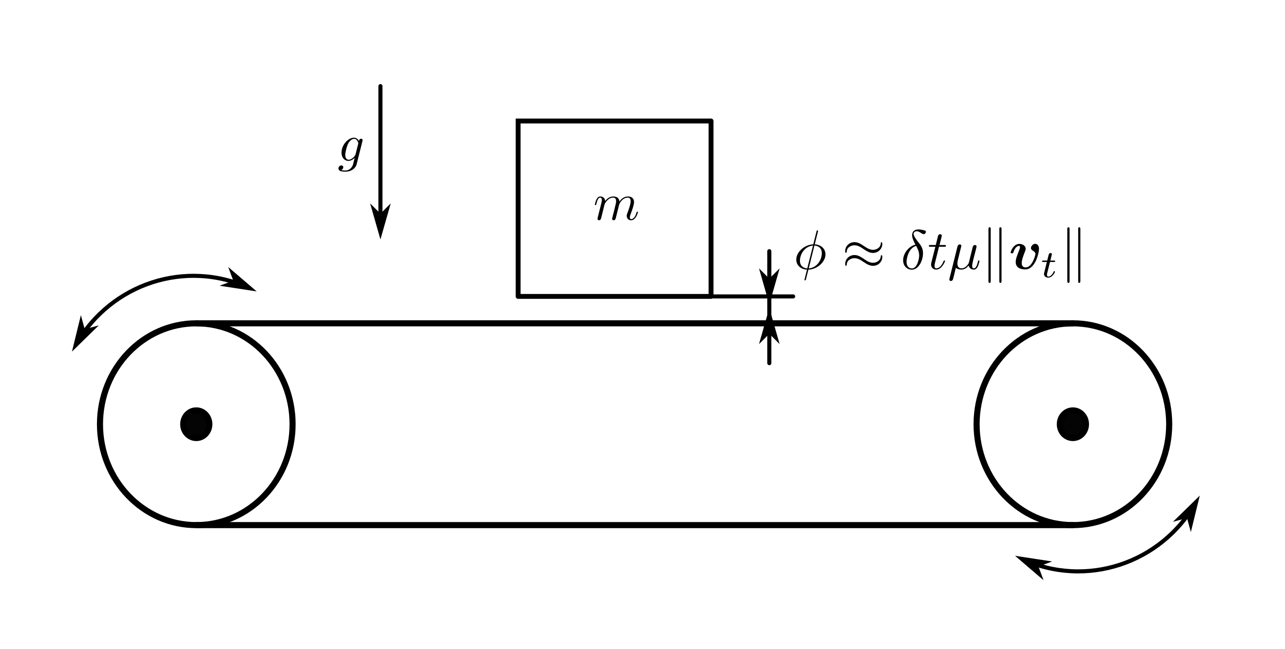
Figure 1: Oscillating Conveyor Belt. The SAP and Similar models suffer from the gliding artifact during slip phases.

Figure 2 shows contact velocity and force computed using a time step of $\delta t=0.01\text{ s}$. Contact between the box and the belt transitions back and forth between stiction and sliding. The Lagged model predicts zero motion in the vertical direction as the normal contact force balances the weight of the box, as expected. However, the SAP and Similar models exhibit noticeable artifacts in the normal direction during the sliding phase, where we observe a non-zero normal velocity due to the non-physical gliding effect introduced by these models. The problem immediately goes away during the stiction phase. We also observe spurious transients in the normal force during the sliding phase — as the slip velocity increases, so does the amount of gliding, which in turn leads to a vertical acceleration and a small change in the normal force. A third spurious effect introduced by the SAP and Similar models are quick changes in the normal force caused by the impulsive transition from sliding into stiction — as soon as the contact transitions to stiction, the gliding artifacts goes to zero, causing a sudden jump in the normal velocity in Fig. 2, accompanied by quick peaks in the normal force.

Figure 2: Contact velocity (left) and force (right) obtained with $\delta t=0.01\text{ s}$.

Figure 3 shows a convergence study with step sizes $\delta t\in\{2\times 10^{-3},10^{-2},5\times 10^{-2}\}$. Both Lagged and Similar exhibit first order convergence, as expected, though the artifacts introduced by Similar (see Fig. 2), cause higher errors than Lagged. Finally, we see in Fig. 3 that SAP’s error starts reaching a plateau at the smallest time step. This is caused by the lack of consistency in the model, for which the term $\tau_{d}\mu\|{\bm{v}}_{t}\|$ in (41) does not vanish as the time step size is reduced.

Since this case quickly reaches a steady state in the normal direction as the contact force balances weight, we do not observe the inconsistent compliance modulation introduced by the Similar model (Section VII-B). We’ll observe this in the test of Section IX-C.

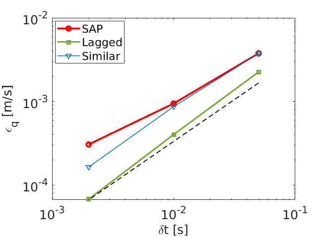
Figure 3: Convergence of the box trajectory with time step size. The dashed line is a reference for first order convergence.

IX-B Falling Sphere

The conveyor belt case in the previous section is the most favorable to the Lagged model given that the normal force is in steady state, and the Lagged model is exact for this condition. Therefore, in this section we introduce a test case with collision, and therefore a sudden change in contact forces, to stress test the performance of the models.

In this case a $0.5\text{ kg}$ steel sphere $5\text{ cm}$ in diameter is let into a free fall from an initial height of $5\text{ cm}$ with an initial horizontal velocity $U_{0}=2\text{ m/s}$, Fig. 4. Friction between the sphere and the ground is $\mu=0.5$. The sphere’s horizontal speed is large enough that when it reaches the ground it first establishes a sliding contact. Friction against the ground imparts angular momentum to the sphere and the contact eventually transitions to a rolling contact. From then on, the friction force is zero and no longer dissipates energy. As before, we model a compliant contact with stiffness $k=10^{7}\text{ N/m}$ and dissipation constants $d=500\text{ s/m}$ and $\tau_{d}=\times 10^{-3}\text{ s}$.

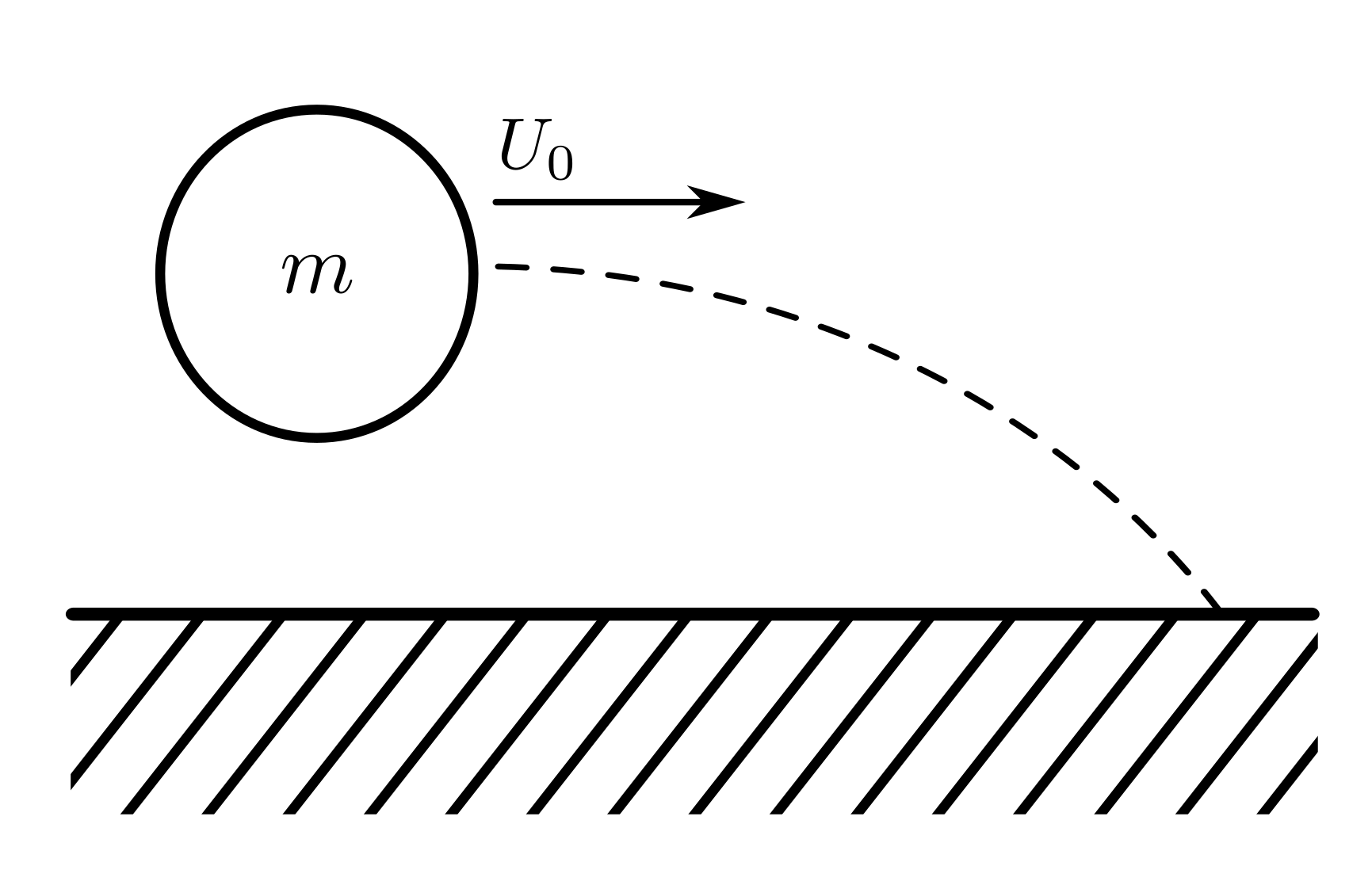
Figure 4: Falling sphere. After a free fall, the sphere slides until friction with the ground establishes a rolling contact.

Figure 5 shows the resulting contact velocity and force for each model using a step size $\delta t=2\times 10^{-3}\text{ s}$. From the forces, we see that both SAP and Similar start making contact earlier. This is due to the action at a distance artifact of these convex approximations. In particular, SAP starts making contact even earlier than the Similar model due to the constant term $\tau_{d}\mu\|{\bm{v}}_{t}\|$ in Eq. (41) that does not vanish as the step size is reduced. In Fig. 5 we see that the cylinder slides from when contact starts until about $t=0.07\text{ s}$, when contact transitions to stiction and the cylinder rolls. While the normal velocity goes to zero almost immediately with the Lagged model, with SAP and Similar models the normal velocity is affected by the slip velocity, and it only goes to zero, as it should, when the contact transitions to stiction. During this transition to from sliding to stiction, we observe the same quick transient on the normal force we observed in the conveyor belt problem. Once again, the Lagged model does not exhibit this artifact.

Figure 5: Contact velocity (left) and force (right) with $\delta t=2\times 10^{-3}\text{ s}$.

A convergence study with step sizes $\delta t\in\{4\times 10^{-4},2\times 10^{-3},10^{-2}\}$ is shown in Fig. 6. While all of these schemes are first order, SAP exhibits a constant error at convergence due to the $\tau_{d}\mu\|{\bm{v}}_{t}\|$ term in (41).

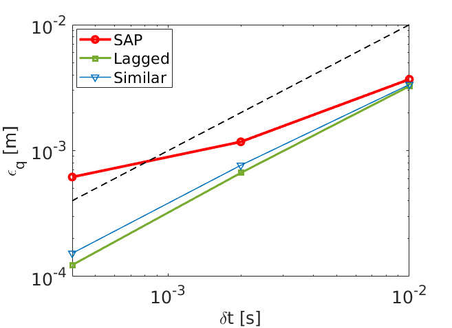
Figure 6: Convergence of the cylinder trajectory with time step size. The dashed line is a reference for first order convergence.

IX-C Sliding Rod

This is a particularly interesting case given that it leads to impact without collision [18, §5.3]. The setup consists of a rod initially forming an angle with the ground making contact at a single point and with a given horizontal velocity, see Fig. 7. As the rod slides, friction makes the rod rotate into the ground leading to an increase in the normal force. Under certain conditions, both normal and frictional forces continue to increase. When formulated at the acceleration level using rigid body assumptions with Coulomb friction, the system can reach a singularity at which contact forces and accelerations are infinity — this is known as Painlevé’s paradox. This problem is resolved in the discrete setting, where finite impulses and discrete changes of velocity are allowed. In the physical world, bodies are not rigid, but real materials deform, vibrate, and even experience plastic (permanent) deformations. Therefore, impulses do not develop in an instant, but rather forces increase to a finite value within a very short period of time. Still, a rapidly increasing contact force develops, an impact, that makes the rod jam into the ground and jump into the air. The rod is $0.5\text{ m}$ in length, $1\text{ cm}$ in diameter and, with a mass of $0.3\text{ kg}$.

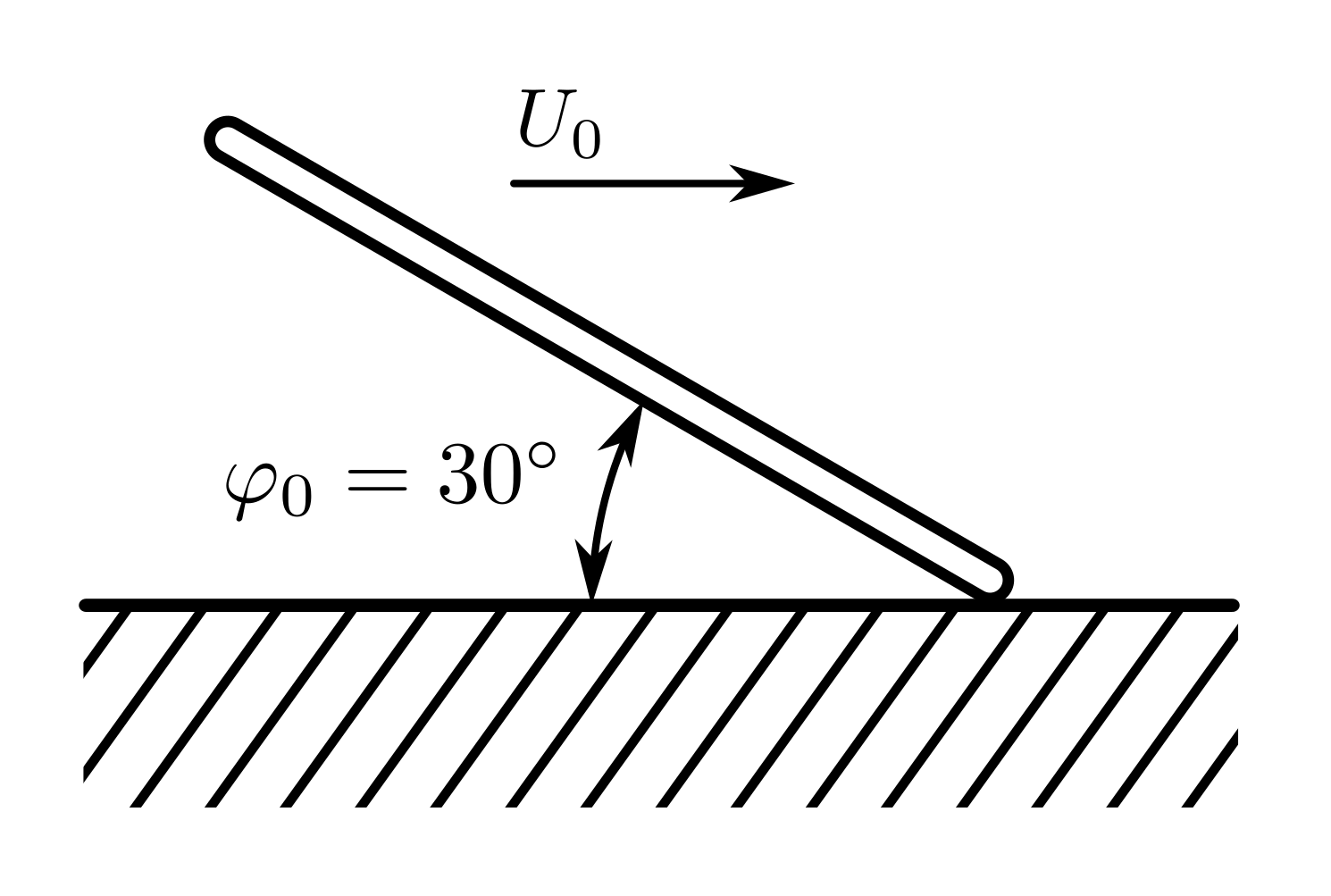
Figure 7: Sliding rod. Initially forming an angle $\varphi_{0}$ with the ground and with horizontal velocity $U_{0}$. Friction makes the rod rotate clockwise. The contact force increases until the rod jams into the ground, making the rod jump into the air.

From analytical analyses [18, §5.3], we know that the singularity can be reached when $\mu>4/3$ and the initial velocity is large enough for the initial kinetic energy to overcome potential energy as the rod’s center of gravity elevates and sliding friction dissipates energy. Therefore, we use a friction coefficient $\mu=2.3$, and set the rod’s initial condition so that it forms a $30^{\circ}$ angle with the ground, see Fig. 7, and it has a horizontal speed of $U_{0}=10\text{ m}/\text{s}$.

We first compute a reference solution with a time step $\delta t=10^{-7}\text{ s}$ and analyze the case with no dissipation in the normal contact force. As predicted from theory, contact with the ground makes the rod rotate upwards as it travels horizontally, forces increase dramatically, and the rod jams into the ground. This can be seen in Fig. 8. All three models produce very similar solutions since without dissipation the compliant model is the same, though with different regularization of friction. We see that before impact the forces oscillate at a frequency determined by the compliance with the ground. Even the location of the impact, which is very sensitive to model parameters, is almost the same for all three models, see inset in Fig. 8.

Figure 8: Contact force in the case with zero dissipation. The figure on the right shows a close up near the impact.

Similarly, we show contact velocities for this case in Fig. 9. The inset shows how the contact moves into the ground due to the large contact force until the tangential component of the velocity becomes zero and the rod jams into the ground. The tangential velocity remains zero during stiction (rather, $\|{\bm{v}}_{t}\|<v_{s}$ since friction is regularized) for a finite period of time of about $0.2\text{ ms}$.

Figure 9: Contact velocity in the case with zero dissipation. The figure on the right shows a close up near the impact.

We run the same simulation with a non-zero Hunt & Crossley dissipation $d=0.2\text{ s}/\text{m}$ and relaxation time $\tau_{d}=4.0\times{10}^{-6}\text{ s}$. These are actually low values of dissipation and we observe in Figs. 10 and 11 that this value of dissipation has very little effect on the time of impact predicted with the Lagged model, our reference solution. Similar and SAP predict a shift on the time of impact, earlier by Similar and later by SAP. Though the predicted contact forces and velocities are quite different with Similar and SAP, we choose the value of $\tau_{d}$ used by SAP so that at least the shift on the time of impact is of the same order as that predicted by the Similar model (though in the opposite direction).

The artifacts introduced by Similar become evident in the inset in Fig. 10, where we observe a frequency shift on the force oscillations. This is caused by the larger effective stiffness of the model during sliding, $k_{\text{eff}}=k\,(1+\mu\|{\bm{v}}_{t}\|\,d)$.

Figure 10: Contact force in the case with dissipation. The figure on the right shows a close up near the impact.

A convergence analysis with and without dissipation is shown in Fig. 12. We use time steps $\delta t=\{6.4\times 10^{-4},1.6\times 10^{-4},4.0\times 10^{-5},1.0\times 10^{-5}\}\text{ s}$. We observe that both SAP and Similar are pretty much indistinguishable when there is no friction. The Lagged model has the most error at the largest simulation time steps, exposing one of the model’s weaknesses. For these rapidly changing solutions, the effect of the lagged normal force in the modeling of Coulomb friction is no longer negligible. We observe that the Lagged model struggles to capture the impact and it even misses it if the time step for this case is larger than about $10^{-3}\text{ s}$. However, the model finally reaches the expected first order convergence regime at the smallest time steps. We observe similar trends for non-zero dissipation, though the curves depart as the prediction of the point of impact changes.

Figure 11: Contact velocity in the case with dissipation. The figure on the right shows a close up near the impact.

Figure 12: Convergence in positions with time step. Case with no dissipation (left) and with dissipation (right).

X Applications

In this section we simulate a number of cases relevant to robotics applications. The purpose is to assess the usefulness of these models for robotics applications, their accuracy, and to evaluate numerical conditioning and performance of the solver.

For all simulations, the solver iterates to convergence, with no early termination or similar procedures to stay within computational budget as commonly done in graphics applications. We use a relative tolerance $\varepsilon_{r}=10^{-5}$ [4].

X-A Clutter

Here we reproduce the clutter case from [4]. In manipulation applications, robots often operate with a cluttered manipuland and therefore the importance to evaluate performance in cases like this. We drop objects into an $80\times 80\times 80\text{ cm}$ box. Objects are initialized into four columns of 10 objects each, totalizing 40 bodies, see Fig 13. Each column consists of an arbitrary assortment of spheres $10\text{ cm}$ in diameter and boxes with sides $10\text{ cm}$ in length. With density of water, spheres have a mass of $0.524\text{ kg}$ and boxes have a mass of $1.0\text{ kg}$. To stress test the solver, we use a very high value of stiffness, $k=10^{7}\text{ N}/\text{m}$, to model steel. Hunt & Crossley dissipation is $d=10\text{ s}/\text{m}$, while SAP’s dissipation is $\tau_{d}=10^{-4}\text{ s}$. For Lagged and Similar we use a tight stiction tolerance of $v_{s}=10^{-4}\text{ m}/\text{s}$, as required for manipulation applications [9, 4]. For SAP and the regularized Lagged model, we use $\sigma=10^{-3}$, also a tight value chosen for manipulation applications [4]. The friction coefficient of all surfaces is $\mu=1.0$, a high value to stress test the solver even further. We let objects fall into the box and simulate for $3$ seconds.

Figure 13: Initial condition (left) and final steady state at $t=3$ seconds (right).

We first study the performance of each method using a time step $\delta t=2\times 10^{-3}\text{ s}$. Figure 14 shows SAP iterations and Hessian condition number at convergence, as a function of time. There is a violent initial transient during which objects undergo impacts as they fall into the box. At about $t=2\text{ s}$ objects still roll around, but the collision phase from the initial fall is over. As expected the solver performs more iterations during this initial violent phase. This is also accompanied by higher condition numbers.

We also observe two distinct features — Both Lagged and Similar models exhibit higher condition number and iterations during this initial transient, while for SAP these are higher past the initial transient. This behaviour is explained by the stiffness $G_{t}$ introduced by the regularized model of friction, see Section VIII. We indeed verify that using the regularized stiction tolerance (44) in the Lagged model conditions the problem better and brings the number of iterations down during this initial transient. Though we did not include it here, the same regularization can be used in the Similar model.

Figure 14: Iterations (left) and condition number (right) as a function of time. $\delta t=2\times 10^{-3}\text{ s}$.

Figure 15 shows the effective stiction tolerance for this case. For the Lagged and Similar models the stiction tolerance is fixed to $v_{s}=10^{-4}\text{ m}/\text{s}$, the dashed black line in the figure. For SAP, and the regularized Lagged model, the effective stiction tolerance changes as a function of the normal impulse, as described in Section VIII. This figure is consistent with the previous observations. During the initial transient the Lagged and Similar models are solving a much tighter approximation of friction. Past this transient, SAP unnecessary solves a much tighter approximation.

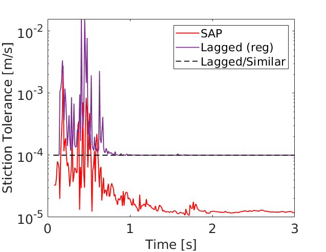
Figure 15: Effective stiction tolerance as a function of time. $\delta t=2\times 10^{-3}\text{ s}$.

An interesting metric is the mean number of iterations and condition number as a function of the time step, shown in Fig. 16. SAP conditioning is essentially independent of the time step, since $G_{t}=1/R_{t}$ in Section VIII is a constant. For the Lagged and Similar models however, conditioning improves as the time step is reduced, since $G_{t}$ is proportional to the impulse, which in turn is proportional to the time step size. This explains why the solver needs fewer iterations to converge for the Lagged and Similar models as the time step is decreased, while it remains quite constant for SAP. Figure 16 also shows the desired effect of regularization for the Lagged model at large time steps. At small time steps, eventually $v_{s}$ dominates in (44) and Lagged with and without regularization performs the same.

Figure 16: Mean number of iterations (left) and condition number (right) per time step as a function of time step size.

Finally, we study the use of compliance as a means to model rigid contact. We measure the mean penetration during the last $1.25$ seconds of simulation, when objects lie in a pile at the bottom of the box. Figure 17 shows this mean steady state penetration as a function of stiffness over a wide range spanning eight orders of magnitude. As a reference, for the spheres $10\text{ cm}$ in diameter in this simulation, Hertz theory predicts an effective stiffness in the order of $10^{7}\text{ N}/\text{m}$ for steel. Therefore, higher stiffness are simply non-physical. However, we stress test our solver with stiffness values up to five orders of magnitude higher, demonstrating the robustness of the convex formulation. We also note, that for a large time step of $\delta t=0.005\text{ s}$ for this case, the near-rigid stiffness estimated by SAP [4] is about $10^{6}\text{ N}/\text{m}$ and still, penetration values are only in the tenths of microns. At $k=10^{13}\text{ N}/\text{m}$ (a non-physical value) the solver fails due to round-off errors. Still, this is six orders of magnitude higher than the stiffness needed to model steel and, for most robotics applications, a lower value in the range $10^{5}-10^{6}\text{ N}/\text{m}$ is more than adequate to approximate rigid contact.

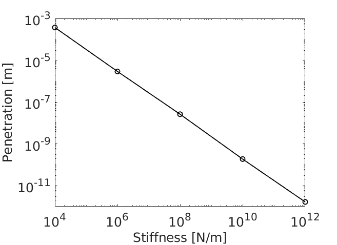
Figure 17: Mean penetration in steady state, during the last $1.25\text{ s}$ of the simulation.

Finally, figure 18 shows the effect stiffness has on the performance of the solver. As expected, higher stiffness values degrade conditioning and this ultimately hurts performance. However, we see that, against common wisdom that prefers rigid contact formulations, the performance changes are only within $20\%$ for stiffness values as high as that of steel.

Figure 18: Mean number of iterations (left) and condition number (right) per time step as a function of stiffness.

Appendix A Soft Norm

We define the soft norm of a vector ${\mathbf{x}}$ as

$$\|{\mathbf{x}}\|_{s}=\sqrt{\|{\mathbf{x}}\|^{2}+\varepsilon_{x}^{2}}-\varepsilon_{x}$$ (45)

where $\varepsilon_{x}>0$ has units of ${\mathbf{x}}$. Notice that $\|{\mathbf{0}}\|_{s}=0$.

The gradient of the soft norm is

$$\frac{\partial\|{\mathbf{x}}\|_{s}}{\partial{\mathbf{x}}}=\frac{{\mathbf{x}}}{\|{\mathbf{x}}\|_{s}+\varepsilon_{x}}=\hat{{\mathbf{x}}}_{s}$$ (46)

where we defined the soft unit vector $\hat{{\mathbf{x}}}_{s}$. This vector has the nice property that numerically, is well defined even at ${\mathbf{x}}={\mathbf{0}}$.

The Hessian of the soft norm, the gradient of $\hat{{\mathbf{x}}}_{s}$, is

$$\frac{\partial\hat{{\mathbf{x}}}_{s}}{\partial{\mathbf{x}}}=\frac{\partial^{2}\|{\mathbf{x}}\|_{s}}{\partial{\mathbf{x}}^{2}} = \frac{1}{\|{\mathbf{x}}\|_{s}+\varepsilon_{x}}\left({\mathbf{I}}-{\mathbf{P}}(\hat{{\mathbf{x}}}_{s})\right)$$ (47)

$$= \frac{{\mathbf{P}}^{\perp}(\hat{{\mathbf{x}}}_{s})}{{\|{\mathbf{x}}\|_{s}+\varepsilon_{x}}}$$

where the projection matrix is defined as ${\mathbf{P}}(\hat{{\mathbf{v}}})=\hat{{\mathbf{v}}}\otimes\hat{{\mathbf{v}}}$. Also ${\mathbf{P}}(\hat{{\mathbf{v}}})\succeq 0$ and ${\mathbf{P}}^{\perp}(\hat{{\mathbf{v}}})\succeq 0$ for all unit vectors $\hat{{\mathbf{v}}}\in\mathbb{R}^{n}$. Therefore the soft norm is twice differentiable with positive semi-definite Hessian, and is therefore convex.

Finally, notice that the expressions for the gradients in Eqs. (45)-(46) are the same as those without softening (i.e. when $\varepsilon=0$). However, these softened versions are convenient in practice because they are well behaved at ${\mathbf{x}}={\mathbf{0}}$ and are continuous.

References

- [1] D. M. Kaufman, S. Sueda, D. L. James, and D. K. Pai, “Staggered projections for frictional contact in multibody systems,” ACM Trans. Graph., vol. 27, no. 5, Dec. 2008.
- [2] M. Anitescu, “Optimization-based simulation of nonsmooth rigid multibody dynamics,” Mathematical Programming, vol. 105, no. 1, pp. 113–143, 2006.
- [3] E. Todorov, “A convex, smooth and invertible contact model for trajectory optimization,” in 2011 IEEE International Conference on Robotics and Automation. IEEE, 2011, pp. 1071–1076.
- [4] A. M. Castro, F. N. Permenter, and X. Han, “An unconstrained convex formulation of compliant contact,” IEEE Transactions on Robotics, 2022.
- [5] H. Mazhar, D. Melanz, M. Ferris, and D. Negrut, “An analysis of several methods for handling hard-sphere frictional contact in rigid multibody dynamics,” Citeseer, Tech. Rep., 2014.
- [6] K. H. Hunt and F. R. E. Crossley, “Coefficient of Restitution Interpreted as Damping in Vibroimpact,” Journal of Applied Mechanics, vol. 42, no. 2, pp. 440–445, 06 1975. [Online]. Available: https://doi.org/10.1115/1.3423596
- [7] A. Pandolfi, C. Kane, J. E. Marsden, and M. Ortiz, “Time-discretized variational formulation of non-smooth frictional contact,” International Journal for Numerical Methods in Engineering, vol. 53, no. 8, pp. 1801–1829, 2002.
- [8] M. Li, Z. Ferguson, T. Schneider, T. R. Langlois, D. Zorin, D. Panozzo, C. Jiang, and D. M. Kaufman, “Incremental potential contact: intersection-and inversion-free, large-deformation dynamics.” ACM Trans. Graph., vol. 39, no. 4, p. 49, 2020.
- [9] A. M. Castro, A. Qu, N. Kuppuswamy, A. Alspach, and M. Sherman, “A transition-aware method for the simulation of compliant contact with regularized friction,” IEEE Robotics and Automation Letters, vol. 5, no. 2, pp. 1859–1866, 2020.
- [10] R. Tedrake and the Drake Development Team, “Drake: Model-based design and verification for robotics,” https://drake.mit.edu, 2019.
- [11] J. Masterjohn, D. Guoy, J. Shepherd, and A. Castro, “Discrete approximation of pressure field contact patches,” 2021, preprint available at https://arxiv.org/abs/2110.04157.
- [12] X. Han, J. Masterjohn, and A. Castro, “A convex formulation of frictional contact between rigid and deformable bodies,” IEEE Robotics and Automation Letters, vol. 8, no. 10, pp. 6219–6226, 2023.
- [13] D. E. Stewart and J. C. Trinkle, “An implicit time-stepping scheme for rigid body dynamics with inelastic collisions and coulomb friction,” International Journal for Numerical Methods in Engineering, vol. 39, no. 15, pp. 2673–2691, 1996.
- [14] M. Anitescu and F. A. Potra, “Formulating dynamic multi-rigid-body contact problems with friction as solvable linear complementarity problems,” Nonlinear Dynamics, vol. 14, no. 3, pp. 231–247, 1997.
- [15] A. Wächter and L. T. Biegler, “On the implementation of an interior-point filter line-search algorithm for large-scale nonlinear programming,” Mathematical programming, vol. 106, pp. 25–57, 2006.
- [16] S. Walker and R. Leine, “Set-valued anisotropic dry friction laws: formulation, experimental verification and instability phenomenon,” Nonlinear Dynamics, vol. 96, pp. 885–920, 2019.
- [17] P. C. Horak and J. C. Trinkle, “On the similarities and differences among contact models in robot simulation,” IEEE Robotics and Automation Letters, vol. 4, no. 2, pp. 493–499, 2019.
- [18] F. Pfeiffer and C. Glocker, Multibody Dynamics with Unilateral Contacts, ser. Wiley Series in Nonlinear Science. Wiley, 1996.