On The Fairness Impacts of Hardware
Selection in Machine Learning

Abstract

In the machine learning ecosystem, hardware selection is often regarded as a mere utility, overshadowed by the spotlight on algorithms and data. This oversight is particularly problematic in contexts like ML-as-a-service platforms, where users often lack control over the hardware used for model deployment. How does the choice of hardware impact generalization properties? This paper investigates the influence of hardware on the delicate balance between model performance and fairness. We demonstrate that hardware choices can exacerbate existing disparities, attributing these discrepancies to variations in gradient flows and loss surfaces across different demographic groups. Through both theoretical and empirical analysis, the paper not only identifies the underlying factors but also proposes an effective strategy for mitigating hardware-induced performance imbalances.

1 Introduction

The leap in capabilities of modern machine learning (ML) models has been powered primarily by the availability of large-scale datasets, gains in available compute, and the development of algorithms that can effectively use these resources (Radford et al., 2019; Brown et al., 2020). As ML-based systems become integral to decision-making processes that bear considerable social and economic consequences, questions about their ethical application inevitably surface. While an active area of research has been devoted to understanding algorithmic choices and their implications on fairness (Hooker et al., 2020; Quan et al., 2023; Caton & Haas, 2020) and robustness (Carlini & Wagner, 2017; Waqas et al., 2022) in neural networks, there has been limited work to date concerning the influence of hardware tooling on these critical aspects of model performance (Hooker, 2020; Zhuang et al., 2022; Jean-Paul et al., 2019).

This inquiry is especially pertinent as the ML hardware landscape undergoes substantial diversification, from successive generations of GPUs, to custom deep-learning accelerators like TPUs (Jouppi et al., 2017). While the hardware landscape is becoming more heterogeneous, the choice researchers have over what hardware they use is often limited. ML models are often trained on ML services or cloud providers where the availability of hardware is determined by factors like cost, geographic location of datacenters and compatibility with ML frameworks (Mince et al., 2023). This introduces the paradox that it is simultaneously more likely a model will be run on multiple hardware types across its lifecycle, but an individual researcher or practitioner has less control over what hardware they are stuck with. It raises the important question: how does varying the type of hardware impact fairness? Importantly, recent studies have indicated that models trained on different hardware can exhibit varying levels of accuracy due to inherent differences in stochasticity (Zhuang et al., 2022). One possible explanation is that hardware-induced nuances, such as precision discrepancies and threading behaviours, may lead iterative optimizers to different local minima during training (Hooker, 2020).

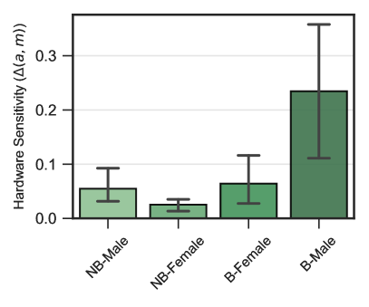
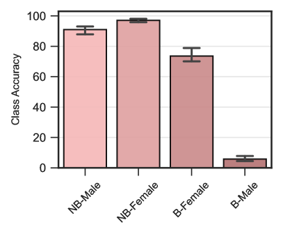
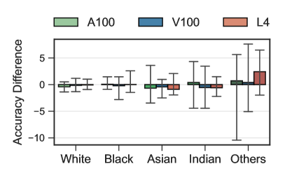
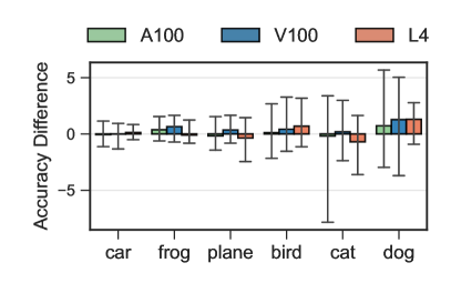
This paper further shows that these hardware-induced variations can disproportionately impact different groups, leading to a “rich get richer, poor get poorer” dynamic. We depict this effect in Figure 1, which shows the variable impact of hardware changes across demographic groups or classes on both a facial recognition task accuracy (left) and on an image classification task (right). Remarkably, while the accuracy rates for majority groups (illustrated with lighter colors) remain relatively stable across different hardware configurations, the rates for minority groups (darker colors) exhibit considerable variability (left plot). This disparity also arises in balanced datasets (right plot).

Figure 1: A model (ResNet34) with the same parameters (random seeds, epochs, batch-size) on different hardware can have vastly different performance results, especially for minority groups (dark colors). The reference hardware is T4. Left: UTK-Face, Right: CIFAR-10.

Building on these observations, this work introduces a theoretical framework aimed at quantifying hardware-induced performance disparities. Both our theoretical treatment and empirical validation reveal that hardware choices systematically alter not just accuracy but also fairness. Our findings suggest that two key mechanisms contribute to these disparities: (1) variations in gradient flows across groups, and (2) differences in local loss surfaces. Informally, the former affects local optimality for groups, while the latter pertains to model separability. We analyze these contributing factors in detail, providing both theoretical and extensive empirical experiments. Additionally, by recognizing these factors, we propose a simple yet effective technique that can be used to mitigate the disparate impacts caused by hardware tooling. The proposed method relies on an alteration to the training procedure to augment the training loss with the factors identified as responsible for unfairness to arise.

Our study stands out for its breadth, conducting experiments that cover a range of hardware architectures, datasets, and model types and the reported results highlight the critical influence of hardware on both performance and ethical dimensions of machine learning models.

2 Related Work

The intersection of hardware selection and fairness in ML is an emerging area of research that has received limited attention. For example, the stochastic effects introduced by software dependencies, such as compilers and deep learning libraries, have been recently shown to impact model performance (Hong et al., 2013; Pham et al., 2020). However, these studies have evaluated these effects within the constraints of specific setups, leaving a gap in understanding how hardware selection affects fairness in machine learning.

In the realm of ML fairness, the focus has predominantly been on algorithmic aspects. Related to our work, the interplay between fairness and efficiency has been examined through the lens of model compression techniques like pruning and quantization (Xu & Hu, 2022; Ahia et al., 2021; Tran et al., 2022). Another possibly related line of work is that which looks at the relationship between fairness and privacy in ML systems. In particular, Differential Privacy (Dwork et al., 2006), an algorithmic property often employed to protect sensitive data in data analytics tasks, has been shown to conflict with fairness objectives. Fioretto et al. (2022) surveys the recent progress in this area, exploring this tension, and suggesting that achieving both privacy and fairness may require careful algorithmic design (Bagdasaryan et al., 2019; Tran et al., 2021a; Cummings et al., 2019; Tran et al., 2021b).

Finally, the influence of randomness introduced through algorithmic choices, including the impact of random seed, initialization, and data handling, has been a focal point of research. Summers & Dinneen (2021) benchmark the separate impact of choices of initialization, data shuffling and augmentation. Ko et al. (2023) evaluate how ensembling can mitigate unfair outcomes. Another body of scholarship has focused on sensitivity to non-stochastic factors including choice of activation function and depth of model (Snapp & Shamir, 2021; Shamir et al., 2020), hyper-parameter choices (Lucic et al., 2018; Henderson et al., 2017; Kadlec et al., 2017; Bouthillier et al., 2021), the use of data parallelism (Shallue et al., 2019) and test set construction (Søgaard et al., 2021; Lazaridou et al., 2021; Melis et al., 2018). While these factors are critical in training phases, they do not study how hardware selection may influence the model outcomes.

Our work aims to bridge this gap, offering new insights into how hardware choices can impact the balance between model performance and fairness. Most relevant to this work is Zhuang et al. (2022) which conducts large-scale experiments across different types of hardware to characterize how tooling choices contribute to the level of non-determinism in a system. Zhuang et al. (2022) analyzes key metrics like churn in predictions to understand the impact of hardware selection on model stability. This work furthers this understanding, by focusing on fairness and providing a theoretical framework to identify the underlying factors but also propose an effective strategy for mitigating hardware-induced performance imbalances. This understanding is crucial for developing more equitable ML systems that consider all facets of the computational environment.

Figure 2: Illustration of the three components in Theorem 1. Left: Difference in model parameter $\rho(m)=\max_{m}^{\prime}\|{\bm{\theta}}^{*}_{m}-{\bm{\theta}}^{*}_{m^{\prime}}\|_{2}$ when $m=T4$. Middle: Gradient flows $\|\bm{g}^{\ell}_{a}\|$ on T4 hardware for five demographic groups $a$. Right: Maximum eigenvalues of the group Hessian $\lambda(\bm{H}^{\ell}_{a,m})$ on T4 hardware for five demographic groups $a$.

3 Preliminaries

We consider a dataset $D$ consisting of $n$ datapoints $(\bm{x}_{i},a_{i},y_{i})$, with $i\in[n]$, drawn i.i.d. from an unknown distribution $\Pi$. Therein, $\bm{x}_{i}\in\mathcal{X}$ is a feature vector, $a_{i}\in\mathcal{A}$ with $\mathcal{A}=[g]$ (for some finite $g$) is a demographic group attribute, and $y_{i}\in\mathcal{Y}$ is a class label. For example, in a face recognition task, the training example feature $\bm{x}_{i}$ may describe a headshot of an individual, the protected attribute $a_{i}$ the individual’s gender or ethnicity, and $y_{i}$ the identity of the individual. The goal is to learn a predictor $f_{\bm{\theta}}:\mathcal{X}\to\mathcal{Y}$, where ${\bm{\theta}}$ is a $k$-dimensional real-valued vector of parameters that minimizes the empirical risk function:

$$\mathrel{\mathop{{\bm{\theta}}}\limits^{\vbox to0.0pt{\kern-2.0pt\hbox{$\scriptstyle\scalebox{0.5}{$\star$}$}\vss}}}\,=\operatorname*{arg\,min}_{\bm{\theta}}J({\bm{\theta}};D)=\frac{1}{n}\sum_{i=1}^{n}\ell(f_{\bm{\theta}}(\bm{x}_{i}),y_{i}),$$ (1)

where $\ell:\mathcal{Y}\times\mathcal{Y}\to\mathbb{R}_{+}$ is a non-negative loss function that measures the model quality. As common in deep learning, we consider iterative optimizers that approximate ${\bm{\theta}}^{*}$ via stochastic gradient descent (SGD) steps ${\bm{\theta}}^{t}={\bm{\theta}}^{t-1}-\eta\bm{g}^{t-1}(B)$. Here $\eta$ denotes the learning rate and $\bm{g}^{t}(B)=\nabla_{{\bm{\theta}}}J(B,{\bm{\theta}}^{t})$ is the gradient of the loss function on a random mini-batch $B$ of samples from $D$.

In this work, our focus is on analyzing the impact of different hardware, used when optimizing the above expression, in relation to the model fairness (as defined next). The paper uses $\mathrel{\mathop{{\bm{\theta}}}\limits^{\vbox to0.0pt{\kern-2.0pt\hbox{$\scriptstyle\scalebox{0.5}{$\star$}$}\vss}}}_{m}$ to denote the parameters of a model training on hardware $m\in\mathcal{M}$, the set of all possible hardware types.

Fairness. The fairness analysis focuses on the notion of hardware sensitivity, defined as the difference among the risk functions of some protected group $a$ of models trained on different hardware from a reference hardware $m$:

$$\Delta(a,m)=\max_{m^{\prime}\in\mathcal{M}}|\mathcal{L}(\mathrel{\mathop{{\bm{\theta}}}\limits^{\vbox to0.0pt{\kern-2.0pt\hbox{$\scriptstyle\scalebox{0.5}{$\star$}$}\vss}}}_{m},D_{a})-\mathcal{L}(\mathrel{\mathop{{\bm{\theta}}}\limits^{\vbox to0.0pt{\kern-2.0pt\hbox{$\scriptstyle\scalebox{0.5}{$\star$}$}\vss}}}_{m^{\prime}},D_{a})|.$$ (2)

Therein, $D_{a}$ denotes the subset of $D$ containing samples ($\bm{x}_{i},a_{i},y_{i}$) whose group membership $a_{i}=a$. Intuitively, the hardware sensitivity represents the change in loss (and thus, in accuracy) that a given group experiences as a result of hardware tooling. Fairness is measured in terms of the maximal hardware loss difference, also referred to as fairness violation across all groups:

$$\xi(D,m)=\max_{a,a^{\prime}\in\mathcal{A}}|\Delta(a,m)-\Delta(a^{\prime},m)|,$$ (3)

defining the largest hardware sensitivity across all protected groups. A fair training method would aim at minimizing the hardware sensitivity across different hardware.

The goal of the paper is to shed light on why fairness issues arise when the only difference in training aspects of a model is the hardware on which the model was trained.

4 Fairness analysis in tooling

To gain insights into how tooling may introduce unfairness, we start by providing a useful bound for the hardware sensitivity of a given group. Its goal is to isolate key aspects of tooling that are responsible for the observed unfairness. The following discussion assumes the loss function $\ell(\cdot)$ to be at least twice differentiable, which is the case for common ML loss functions, such as mean squared error or cross-entropy loss. We report proofs of all theorems in Appendix A.

Figure 3: Illustration of Impact of group size on Gradient Norm Imbalance as shown in Theorem 3. Left: Group size used in training for five demographic groups. Middle: Gradient flows $\bm{g}_{a}$ for 5 different demographic groups $a$ averaged across three devices with 10 seeds each. Right: Hardware Sensitivity; Notice higher sensitivity as the group size decreases.

Theorem 1.

Given reference hardware $m$, the hardware sensitivity $\Delta(a,m)$ of group $a\in\mathcal{A}$ is upper bounded by:

$$\begin{split}\Delta(a,m)\leq&\left\|\bm{g}_{a,m}^{\ell}\right\|\times\rho(m)+\frac{1}{2}\lambda\left(\bm{H}_{a,m}^{\ell}\right)\times\rho(m)^{2}+\mathcal{O}\left(\rho(m)^{3}\right)\end{split}$$ (4)

where $\rho(m)=\max_{m\in\mathcal{M}}\|{\bm{\theta}}^{*}_{m}-{\bm{\theta}}^{*}_{m^{\prime}}\|_{2}$ is the largest difference of the model parameters associated with model $m$ and a reference model $m^{\prime}$, $\bm{g}_{a,m}^{\ell}=\nabla_{{\bm{\theta}}}J(\mathrel{\mathop{{\bm{\theta}}}\limits^{\vbox to0.0pt{\kern-2.0pt\hbox{$\scriptstyle\scalebox{0.5}{$\star$}$}\vss}}}_{m};D_{a})$ are the gradient values associated with the samples of group $a$, and $\bm{H}_{a,m}^{\ell}=\nabla^{2}_{{\bm{\theta}}}J(\mathrel{\mathop{{\bm{\theta}}}\limits^{\vbox to0.0pt{\kern-2.0pt\hbox{$\scriptstyle\scalebox{0.5}{$\star$}$}\vss}}}_{m};D_{a})$ is the Hessian of the loss function associated with group $a$, with $\lambda(\Sigma)$ as the maximum eigenvalue of matrix $\Sigma$.

Figure 4: Upper bound (green) vs RHS components of Equation 4 (blue).

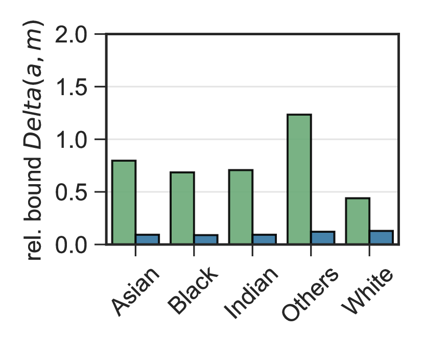
The upper bound is derived using a second-order Taylor expansion, the Cauchy-Schwarz inequality, and Rayleigh quotient properties.

Firstly, empirically, we find that this upper bound closely approximates the hardware sensitivity in practice. This tightness of the bound is illustrated in Figure 4, where we also show that the contribution of the third-order term in Equation (4) is negligible. This empirical validation is consistent with observations in existing literature (Vadera & Ameen, 2022; Gu & Guo, 2021).

Next, we note that the constant factor $\rho(m)$ is non-zero, as evidenced by Figure 2 (left). These two observations emphasize the presence of two key group-dependent terms in Equation 4 that modulate hardware sensitivity and form the crux of our fairness analysis. Specifically, they are (1) the norms of the gradients $\bm{g}_{a,m}^{\ell}$ (also called, gradient flows) and (2) the maximum eigenvalue of the Hessian matrix $\bm{H}_{a,m}^{\ell}$ for a given group $a$ and reference hardware $m$, also called group Hessian throughout the paper. Informally, the first term relates to the local optimality within each group, whereas the second term is indicative of the model’s capacity to distinguish between different groups’ data. Figure 2 provides an illustration of the disparity of these components across protected groups. We will subsequently demonstrate that these components serve as the primary sources of unfairness attributed to tooling.

The next sections analyze the effect of varying hardware types on both gradient flows and the group Hessian. This understanding, besides clarifying the roles of these components onto (un)fairness, will help us design an effective mitigation technique, introduced in Sec. 7.

4.1 Group Gradient Flows

Theorem 1 illustrates that a key determinant of unfairness in hardware selection lies in the differences in gradient flows across groups. It points out that larger gradient flows for a given group are associated with increased hardware sensitivity for that group.

To delve deeper into this issue we look into a property of the training data. Our observations indicate that the size of the training group plays a significant role in these disparities. Theorem 2 explores this phenomenon in binary group settings, illustrating how differences in group sizes can lead to distinct gradient norms. Theorem 3 broadens the scope of this analysis to multi-group contexts, under mild assumptions.

Theorem 2.

Consider a local minimum ${\bm{\theta}}^{*}_{m}$ of Equation (1) on a reference hardware $m\in\mathcal{M}$ and let the set of protected groups be $\mathcal{A}=\{a,b\}$. If $|D_{a}|>|D_{b}|$ then $\|\bm{g}_{a}\|<\|\bm{g}_{b}\|$.

The proof is derived by leveraging the conditions for a local minimum and the proportional contributions of each group to the total gradient. This result explains why smaller groups yield larger gradient norms, which consequently amplify sensitivity to stochasticity introduced by hardware, as observed in our experimental results. We next generalize these insights to arbitrary group sets $\mathcal{A}$.

Theorem 3.

Consider a hardware configuration $m$ and denote $\underline{a}=\min_{a\in\mathcal{A}}|D_{a}|$ to be the most underrepresented group. Suppose that for any group $a,a^{\prime}\in\mathcal{A}\setminus\{\underline{a}\}$ the angle between their gradient vectors $\overrightarrow{\bm{g}_{a}},\overrightarrow{\bm{g}_{a^{\prime}}}$ is less than $\frac{\pi}{2}$. Then $\|\bm{g}_{\underline{a}}\|=\max_{a\in\mathcal{A}}\|\bm{g}^{\ell}_{a}\|$

Theorem 3 suggests that the group with the smallest number of training samples will exhibit the largest gradient norm upon convergence. The underlying assumption—that the angle between any pair of gradient vectors is less than $\frac{\pi}{2}$— essentially posits that the learning tasks across different groups are not highly dissimilar, which is often observed in practice (Guangyuan et al., 2022).

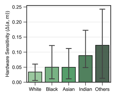
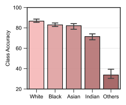
This influence of group size on gradient norm is exemplified in Figure 3. Within the UTK-Face dataset, the White category has the highest number of training samples, while Others has the fewest (left plot). Consequently, the majority group (White) exhibits the smallest gradient norm, while the group Others shows the largest (Figure 3 middle). As corroborated by Theorem 1, which establishes the link between gradient norm and hardware sensitivity (unfairness), the majority group manifests the least sensitivity, whereas the minority one has the highest. This is illustrated in the right subplot of Figure 3. Additional empirical evidence supporting the impact of group sizes on gradient norms is provided in Section 6.

4.2 Group Loss Landscape

While the previous section reviewed the influence of gradient flows on the unfairness observed in tooling, Theorem 1 introduces another critical variable in determining hardware sensitivity: the eigenvalues of the group Hessians. Intuitively, the group Hessian serves as an indicator for the flatness of the loss landscape around the optimal solution (Li et al., 2018), as well as for the model’s generalization capability (Kaur et al., 2023).

Figure 5: Illustration on the impact of group Hessians. Group ’a’ has a smaller Hessian compared to Group ’b’, resulting in lower sensitivity of the loss function for Group ’a’.

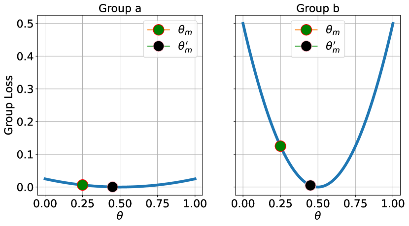
For illustrative purposes, Figure 5 represents how differences in Hessian’s maximum eigenvalues impact hardware sensitivity. In this example, group $a$ has a flatter loss landscape around the stationary point compared to group $b$ due to its smaller group Hessians. As a result, variations in model parameters ${\bm{\theta}}^{*}_{m}$ and ${\bm{\theta}}^{*}_{m^{\prime}}$ across hardwares $m$ and $m^{\prime}$ lead to a much smaller change in the loss function for group $a$ than for group $b$. This difference underscores the direct link between the group Hessian’s maximum eigenvalues and the degree of hardware sensitivity experienced by each group.

The next result shed light on the underlying reasons for the observed disparities in group-specific Hessians. Theorem 4 establishes a relationship between the maximum eigenvalues of the group Hessian and the average distance of samples within that group to the decision boundary.

Theorem 4.

Consider a model $f_{{\bm{\theta}}^{*}_{m}}$ trained using binary cross entropy on reference hardware $m$. Then, $\forall a\in\mathcal{A}$, the maximum eigenvalue of the group Hessian $\lambda(\bm{H}_{a}^{\ell})$ is bounded by:

$$\lambda(\bm{H}_{a}^{\ell}) \leq\frac{1}{|D_{a}|}\sum_{(\bm{x},y)\in D_{a}}\delta_{\bm{x}}\times\left\|\nabla_{{\bm{\theta}}}f_{{\bm{\theta}}^{*}_{m}}(\bm{x})\right\|^{2}\quad+\left|f_{{\bm{\theta}}^{*}_{m}}(\bm{x})-y\right|\times\lambda\left(\nabla^{2}_{{\bm{\theta}}}f_{{\bm{\theta}}^{*}_{m}}(\bm{x})\right),$$

where $\delta_{\bm{x}}=\left({f}_{{\bm{\theta}}^{*}_{m}}(\bm{x})\right)\left(1-{f}_{{\bm{\theta}}^{*}_{m}}(\bm{x})\right)$ is the distance to decision boundary and ${f}_{{\bm{\theta}}}(\bm{x})\in[0,1]$ is the output obtained after the last Sigmoid layer.

This theorem relies on derivations of the Hessian associated with the model loss function and Weyl inequality provided in Theorem 2. In other words, Theorem 4 shows that the maximum eigenvalue of the group-specific Hessian is directly linked to how close the samples from that group are to the decision boundary, as measured by the term ${f}_{{\bm{\theta}}^{*}_{m}}(\bm{x})(1-{f}_{{\bm{\theta}}^{*}_{m}}(\bm{x}))$. Intuitively, this term is at its maximum when the classifier is most uncertain about its prediction, meaning when ${f}_{{\bm{\theta}}^{*}_{m}}(\bm{x})$ is close to 0.5. Conversely, it reaches a minimum when the classifier is most certain, that is, when ${f}_{{\bm{\theta}}^{*}_{m}}(\bm{x})$ approaches either 0 or 1 in this binary classification setting. This relationship is further elaborated in Proposition 2.1 (see appendix).

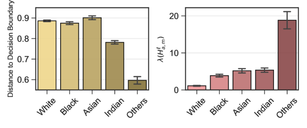
An empirical illustration, shown in Figure 6, highlights the relationship between group Hessian eigenvalues and proximity to the decision boundary. Notice how samples from the Others group are closer to the decision boundary, indicating that they are less separable than those in other groups. As a result, this group reports the largest eigenvalue of group Hessians. Similar observations on other datasets are discussed in the following section.

Figure 6: The relationship between the group Hessian and distance to the decision boundary.

Having discussed the main reasons justifying unfairness in hardware selection, the next sections delve into empirical validation and discuss a possible mitigation solution.

5 Experimental Setup

We first review the experimental setup.

Hardware selection. We report experiments across widely adopted GPU types: Tesla T4 (NVIDIA, 2018a), Tesla V100 (NVIDIA, 2017a), Ampere A100 (NVIDIA, 2021) and Ada L4 GPU (NVIDIA, 2023). These hardware types differ in CUDA core count, total threads and streaming multiprocessors (refer to Table 1 in the appendix for more details). Hardware characteristics impact the overall level of stochasticity introduced by different hardware types. GPUs introduce stochasticity due to random floating-point accumulation ordering from parallel threads, which often cause inconsistent outputs between multiple runs due to the truncation of fraction part in floating point number in the accumulation procedure (Chou et al., 2020). Respectively, A100, L4, V100, and T4 GPUs are each equipped with varying numbers of CUDA cores (6912, 7424, 5120, and 2560, respectively) for floating-point computations. These differences in parallelization relate to the design choices of the hardware, for example, the T4 and L4 GPUs were specifically designed for inference workloads which often present lower memory bandwidth requirements.

Controlling other sources of stochasticity. To ensure that our analysis focuses solely on the impact of hardware on model fairness and performance, we have kept all other variables constant and deterministic. This is done by fixed randomness for all Python libraries adopted, and maintaining consistent data loading and augmentations, using FFCV-SSL (Bordes et al., 2023). This controlled environment ensured that the same stochastic elements were present during both the training and inference stages. Additionally, we maintained consistency in library versions and for CUDA cores (Chetlur et al., 2014) experiments we consistently used the same precision FP32 for all accumulators, except in the case of the CelebA dataset where we used mixed-precision training. Finally, all results report average and standard deviation of metrics reported over multiple random seeds. This approach allows us to confidently attribute any observed variations in sensitivity or stochasticity specifically to the unique characteristics of the hardware platform.

Datasets. The experiments use three datasets: CIFAR-10 (Krizhevsky, 2009), CelebA (Liu et al., 2015), and UTKFace (Zhang et al., 2017). UTKFace and CelebA are naturally unbalanced datasets, while CIFAR-10 is a balanced dataset. To examine the impact of class imbalance in the CIFAR dataset, we also created an Imbalanced version where class 8 (Ship for CIFAR-10) constitutes only $20\%$ of its original size, with other classes remaining unchanged. We reformulate the task for CelebA such that there are 4 classes based on the presence of the ’male’ and blond-hair’ attributes. This leads to an imbalanced dataset for multi-class instead of multi-label classification tasks. For tasks related to UTKFace, we use the ethnicity label as the ground truth while training. We include a more extensive description of each dataset and additional details about task structure in Appendix B.1.

Architectures. Finally, in addition to multiple hardware, hyper-parameters, and datasets, we also evaluate our results on four different architectures with increasing complexity SmallCNN, ResNet18, ResNet34 and ResNet50 (He et al., 2015) (see Appendix B.2 for additional details). This allow us to validate our theoretical findings over a broad range of settings. All the models have been trained using the SGD optimizer with momentum $0.99$, and weight deacy of $5e-4$ a three-phase One Cycle LR (Leslie, 2015) scheduler with a starting learning rate of $0.1$. The batch size for CIFAR10 was 512, for UTKFace it was 32 for ResNet50 and 128 for other models; For CelebA batch size was 200. For CIFAR10 and CelebA the model was trained for 15 epochs. In the case of UTKFace Ethnicity the model was trained for 20 epochs. We used automatic mixed-precision training for CelebA via torch.amp with float16 as the intermediate data type due to increased memory requirements.

6 Experimental Results

Our fairness analysis relies on the notion of hardware sensitivity, as defined in Equation (2). Recall that this metric measures the maximum difference in class loss between a model trained on a reference hardware and models trained on various other hardware setups, while keeping all other parameters unchanged. The notion of hardware sensitivity helps us understand the theoretical impact of hardware on model performance. However, ultimately we are interested in measuring the accuracy variations across classes due to varying tooling for training. Hence, in this section, we will also examine how varying hardware contributes to differences in accuracy across different groups. When looking at hardware sensitivity, small values indicate more consistent results across hardware.

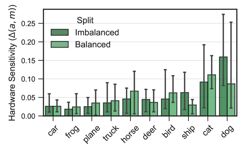
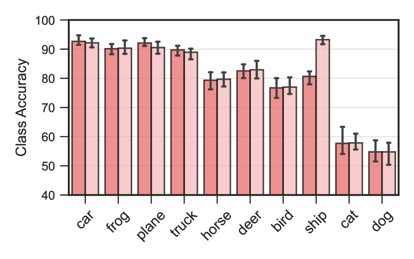
In the experiments conducted across Tesla T4, Tesla V100, Ampere A100, and Ada L4 architectures, we found notable fairness (hardware sensitivity) variations. Figure 7 illustrates this for the CIFAR10 dataset. Firstly, observe that larger hardware sensitivity values for a class are associated with greater deviations in that class’s accuracy. Next, also notice that classes showing smaller hardware sensitivity (indicative of greater fairness) tend to be those with higher overall accuracies. To gain a better understanding of these trends, let us examine the hardware sensitivity of class 8 (Ship) under both balanced and imbalanced scenarios, as depicted in Figure 7 (top). In the imbalanced setting, where class 8 had five times fewer samples than other classes, there is a notable 57% increase in hardware sensitivity for the Ship class.

This pattern is not unique to a single dataset. For instance, in the UTKFace dataset, the minority class Others exhibits 91% higher hardware sensitivity compared to the majority class White as depicted in Figure 12 in the Appendix. Similarly, in the CelebA dataset, the blond-male minority class presents hardware sensitivity that is 76% more than that of the non-blond female majority class, as shown in Figure 11 in the Appendix. These observations support our hypothesis that hardware selection can disproportionately affect the performance of minority classes.

Figure 7: Left: Hardware sensitivity for CIFAR10 (ResNet34) Balanced and Imbalanced. Right: Class-wise accuracy. High Fairness violations are noted for the Imbalanced CIFAR10.

6.1 Gradient Flows

We now turn our attention to the influence of gradient flows on the disparities in accuracy resulting from hardware selection. As established in Theorem 1, the magnitude of gradient flow within a group is directly linked to its hardware sensitivity. The norm of the group’s gradients, or their gradient flows, is indicative of the local optimality of the model for a group. Essentially, this term measures how sensitively the model responds to the specific characteristics within the data of each demographic group. Larger gradient norm values suggest that the model is less optimized for that particular group, implying a greater potential for accuracy disparities due to hardware selection.

Figure 8 illustrates the relationship between the group gradient flows and the hardware sensitivity. Notice the strong correlation between a group’s hardware sensitivity and its gradient flow, particularly under conditions of imbalance. In CIFAR10, in particular, unbalancing class Ship (five times fewer samples) results in a 62.6% increase in the gradient norm and a corresponding rise in hardware sensitivity by 57%. This trend is also echoed in the UTKFace-ethnicity task, where the gradient norm of the minority class Others is significantly higher 95.2% more than the majority class White. The CelebA dataset shows a similar pattern; the minority class blond-male exhibits a gradient norm 99.177% more than the majority class non-blond-female.

Figure 8: Correlation plot between Hardware sensitivity and gradient flows. 1st: Even with a perfectly balanced dataset, classes with higher gradient flows tend to have higher sensitivity in the change of hardware. 2nd: Class 8 (Ship) is imbalanced in this setting and sees a sharp increase in its gradient norm and sensitivity. 3rd:There is a strong correlation between the gradient norm of groups and the hardware sensitivity in the ascending order of imbalance for UTKFace. 4th: A similar trend is also found for the CelebA classification task.

These observations highlight the impact of class imbalance on gradient norms and hardware sensitivity, reinforcing the idea that minority classes tend to exhibit higher sensitivity to hardware variations, which in turn can affect the accuracy of the model for these specific groups.

6.2 Distance to the Decision Boundary

Next, we look at the second factor of unfairness highlighted in Theorem 1: the effect of the maximum eigenvalue of the group Hessian. Such values provide insight into the model’s capacity to differentiate between the data of different groups. A larger maximum eigenvalue implies that the model’s loss surface is more curved for the data of that particular group. This curvature is indicative of how sensitive the model is to variations in the data belonging to that group. Theorem 4 further links this component with the distance to the boundary, and we show next how such notion connects to hardware sensitivity (unfairness).

Figure 9: 1st: Distance-to-decision Boundary for UTKFace Ethnicity on ResNet34. 2nd: Class-wise accuracy. 3rd: Distance-to-decision Boundary for CelebA on ResNet34. 4th: Class-wise accuracy.

Figure 9 illustrates the relationship between the distance to decision boundary and hardware sensitivity for the UTK Face and the CelebA datasets. We adopt the definition of distance to the decision boundary from Tran et al. (2021a). For each sample $\bm{x}$, this distance is computed as $\delta_{\bm{x}}=1-\sum_{i=1}^{|\mathcal{Y}|}p^{2}_{i}(\bm{x})$, where $p_{i}(\bm{x})$ represents the softmax probability distribution of $\bm{x}$, with values ranging between 0 and 1. Notably, the average distance to the decision boundary is a strong predictor of hardware sensitivity. In cases involving a minority class, such as Others in the UTK Face dataset, this distance is significantly shorter (67% lower) compared to other classes like White (see first and second subplots). On CelebA (third and fourth subplots), the average distance to the decision boundary is 61.28% lower for blond-male compared to non-blond-female. These findings align with the theoretical implications presented in our paper.

7 Mitigation solution

Given the influence of the groups’ gradient flows and group Hessians on the model unfairness due to hardware selection, one intuitive approach to mitigate the observed effects is to equalize the gradient and Hessian values across groups during training. However, this approach is computationally intensive and often impractical, especially for large models, primarily due to the challenges in computing the Hessian matrix during backpropagation. To address this issue, we propose a more efficient mitigation strategy, underpinned by the observations provided in Proposition 2.1 (see Appendix). This proposition elucidates the relationship between the group Hessian and the distance to the decision boundary. Leveraging this insight, our approach aims to align the average distance to the decision boundary among different groups.

Figure 10: Left: Accuracy Difference for groups pre and post-mitigation for UTKFace Ethnicity on ResNet18. Notice the Maximum Accuracy Difference between the maximum and minimum accuracy within groups is reduced by 66% from 2.92 to 0.99, post-mitigation averaged across hardware. Right: Accuracy Difference for groups pre and post-mitigation for CIFAR10 Imbalanced on ResNet18. Notice the Maximum Accuracy Difference between the maximum and minimum accuracy within groups is reduced by 28%, from 1.916 to 1.366, post-mitigation averaged across hardware.

We achieve this by augmenting the empirical risk function with a component that quantifies the disparity between the group-specific and batch-wide distances to the decision boundary:

$$\mathrel{\mathop{{\bm{\theta}}}\limits^{\vbox to0.0pt{\kern-2.0pt\hbox{$\scriptstyle\scalebox{0.5}{$\star$}$}\vss}}}_{F}\,=\operatorname*{arg\,min}_{\bm{\theta}}J({\bm{\theta}};D)+\lambda\sum_{a\in\mathcal{A}}(\delta_{\mathcal{D}_{a}}-\delta_{\mathcal{D}})^{2},$$ (5)

where $\delta_{S}$ represents the average distance to the decision boundary of samples $\bm{x}\in S$ as described in the Section 6.2, and $\lambda$ is a hyper-parameter which calibrates the level of penalization.

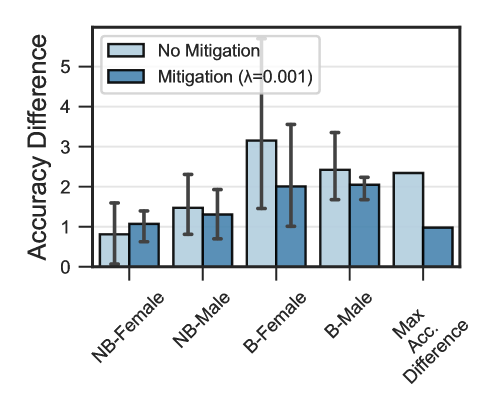
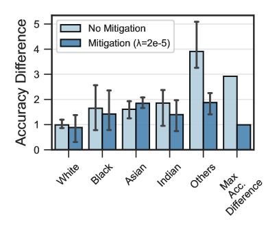
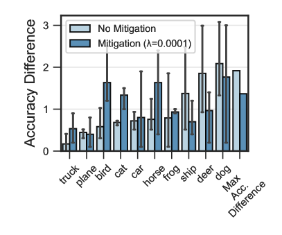
In our experiments, we implemented this mitigation strategy across various hardware setups and observed a significant reduction in accuracy difference as outlined in Section 3. While it is possible to optimize the choice of the value $\lambda$ during the empirical risk process, e.g., using a Lagrangian dual approach as in (Fioretto et al., 2020a, b), we found that even a traditional simple grid search allows us to find good $\lambda$ values yielding an effective reduction in accuracy disparity. Figure 10 shows a marked decrease in maximum difference in accuracy within various groups for the UTK Face dataset (left) and CIFAR10 (right). Additional results on CelebA are reported in Figure 13 (Appendix) and display similar trends. It is to be noted that for each dataset, different $\lambda$ values produced different reductions in accuracy difference.

Specifically, for a ResNet50 model trained on the CelebA dataset, the implementation of our mitigation scheme resulted in a 38% reduction in maximum difference in accuracy within groups, decreasing from 2.34 to 0.936. It also reduces the average accuracy difference across multiple hardware as indicated in the right subplot in Figure 13. The biggest reduction of the maximum difference in accuracy within groups was noticed in the UTKFace Ethnicity dataset on ResNet18 Model for $\lambda=2e-5$. The reduction was 66% from 2.92 to 0.99.

These results highlight the effectiveness of our proposed method in addressing fairness concerns attributable to hardware variations.

8 Conclusion

This paper focused on an often overlooked aspect of responsible ML models: How variations in hardware can disproportionately affect different demographic groups. We’ve presented a theoretical framework to quantitatively assess these hardware-induced disparities, pinpointing variations in gradient flows across groups and differences in local loss surfaces as primary factors contributing to these disparities. These findings have been validated by extensive empirical studies, carried out on multiple hardware platforms, datasets, and architectures.

The findings of this study are significant: the sensitivity of model performance to specific hardware choices can lead to unintended negative societal outcomes. For example, organizations that release their source codes and model parameters may attest to satisfactory performance levels for certain demographic groups, based on results from their chosen training hardware. However, this claimed performance could substantially degrade when the models are implemented on different hardware platforms. Our work thus serves as both a cautionary tale and a guide for responsible practices in reporting across diverse hardware settings.

Ethical considerations

The analyses and solutions reported in this paper should not be intended as an endorsement for using the developed techniques to aid facial recognition systems. We hope this work creates further awareness of the unfairness caused by variations in data, model, and hardware setup.

Supplemental Material

Appendix A Missing proofs

Theorem 1.

Given a reference hardware $m$, the hardware sensitivity of a group $a\in\mathcal{A}$ is upper bounded by:

$$\Delta(a,m) \leq\left\|\bm{g}_{a,m}^{\ell}\right\|\times\max_{m^{\prime}\in\mathcal{M}}\left\|\mathrel{\mathop{{\bm{\theta}}}\limits^{\vbox to0.0pt{\kern-2.0pt\hbox{$\scriptstyle\scalebox{0.5}{$\star$}$}\vss}}}_{m}-\mathrel{\mathop{{\bm{\theta}}}\limits^{\vbox to0.0pt{\kern-2.0pt\hbox{$\scriptstyle\scalebox{0.5}{$\star$}$}\vss}}}_{m^{\prime}}\right\|+\frac{1}{2}\lambda\left(\bm{H}_{a,m}^{\ell}\right)\times\max_{m^{\prime}\in\mathcal{M}}\left\|\mathrel{\mathop{{\bm{\theta}}}\limits^{\vbox to0.0pt{\kern-2.0pt\hbox{$\scriptstyle\scalebox{0.5}{$\star$}$}\vss}}}_{m}-\mathrel{\mathop{{\bm{\theta}}}\limits^{\vbox to0.0pt{\kern-2.0pt\hbox{$\scriptstyle\scalebox{0.5}{$\star$}$}\vss}}}_{m^{\prime}}\right\|^{2}$$ (6)

$$+\mathcal{O}\left(\max_{m^{\prime}\in\mathcal{M}}\left\|\mathrel{\mathop{{\bm{\theta}}}\limits^{\vbox to0.0pt{\kern-2.0pt\hbox{$\scriptstyle\scalebox{0.5}{$\star$}$}\vss}}}_{m}-\mathrel{\mathop{{\bm{\theta}}}\limits^{\vbox to0.0pt{\kern-2.0pt\hbox{$\scriptstyle\scalebox{0.5}{$\star$}$}\vss}}}_{m^{\prime}}\right\|^{3}\right),$$

where $\bm{g}_{a,m}^{\ell}=\nabla_{{\bm{\theta}}}J(\mathrel{\mathop{{\bm{\theta}}}\limits^{\vbox to0.0pt{\kern-2.0pt\hbox{$\scriptstyle\scalebox{0.5}{$\star$}$}\vss}}}_{m};D_{a})$ is the vector of gradients associated with the loss function $\ell$ evaluated at $\mathrel{\mathop{{\bm{\theta}}}\limits^{\vbox to0.0pt{\kern-2.0pt\hbox{$\scriptstyle\scalebox{0.5}{$\star$}$}\vss}}}_{m}$ and computed using group data $D_{a}$, $\bm{H}_{a,m}^{\ell}=\nabla^{2}_{{\bm{\theta}}}J(\mathrel{\mathop{{\bm{\theta}}}\limits^{\vbox to0.0pt{\kern-2.0pt\hbox{$\scriptstyle\scalebox{0.5}{$\star$}$}\vss}}}_{m};D_{a})$ is the Hessian matrix of the loss function $\ell$, at the optimal parameters vector $\mathrel{\mathop{{\bm{\theta}}}\limits^{\vbox to0.0pt{\kern-2.0pt\hbox{$\scriptstyle\scalebox{0.5}{$\star$}$}\vss}}}_{m}$, computed using the group data $D_{a}$ (henceforth simply referred to as group hessian), and $\lambda(\Sigma)$ is the maximum eigenvalue of a matrix $\Sigma$.

Proof.

Using a second order Taylor expansion around ${\bm{\theta}}^{*}_{m}$, the change in loss function of one particular group $a$ when it is trained on another hardware $m^{\prime}\in\mathcal{M}$ can be approximated as:

$$J({\bm{\theta}}^{*}_{m^{\prime}};D_{a})-J({\bm{\theta}}^{*}_{m};D_{a}) =J\left({\bm{\theta}}^{*}_{m};D_{a}\right)+\left({\bm{\theta}}^{*}_{m^{\prime}}-{\bm{\theta}}^{*}_{m}\right)^{\top}\,\nabla_{\theta}J\left({\bm{\theta}}^{*}_{m};D_{a}\right)$$

$$\hskip 15.0pt+\frac{1}{2}\left({\bm{\theta}}^{*}_{m^{\prime}}-{\bm{\theta}}^{*}_{m}\right)^{\top}\,\bm{H}_{a}^{\ell}\left({\bm{\theta}}*_{m^{\prime}}-{\bm{\theta}}^{*}_{m}\right)+\mathcal{O}\left(\max_{m^{\prime}\in\mathcal{M}}\left\|\mathrel{\mathop{{\bm{\theta}}}\limits^{\vbox to0.0pt{\kern-2.0pt\hbox{$\scriptstyle\scalebox{0.5}{$\star$}$}\vss}}}_{m}-\mathrel{\mathop{{\bm{\theta}}}\limits^{\vbox to0.0pt{\kern-2.0pt\hbox{$\scriptstyle\scalebox{0.5}{$\star$}$}\vss}}}_{m^{\prime}}\right\|^{3}\right)-J\left({\bm{\theta}}^{*}_{m};D_{a}\right)$$

$$=\left({\bm{\theta}}^{*}_{m^{\prime}}-{\bm{\theta}}^{*}_{m}\right)^{\top}\,\bm{g}^{\ell}_{a}+\frac{1}{2}\left({\bm{\theta}}^{*}_{m}-{\bm{\theta}}^{*}_{m}\right)^{\top}\,\bm{H}_{a}^{\ell}\left({\bm{\theta}}^{*}_{m^{\prime}}-{\bm{\theta}}^{*}_{m}\right)+\mathcal{O}\left(\max_{m^{\prime}\in\mathcal{M}}\left\|\mathrel{\mathop{{\bm{\theta}}}\limits^{\vbox to0.0pt{\kern-2.0pt\hbox{$\scriptstyle\scalebox{0.5}{$\star$}$}\vss}}}_{m}-\mathrel{\mathop{{\bm{\theta}}}\limits^{\vbox to0.0pt{\kern-2.0pt\hbox{$\scriptstyle\scalebox{0.5}{$\star$}$}\vss}}}_{m^{\prime}}\right\|^{3}\right)$$ (7)

The above, follows from the loss $\ell(\cdot)$ being at least twice differentiable, by assumption.

By Cauchy-Schwarz inequality, it follows that:

$$\left({\bm{\theta}}^{*}_{m^{\prime}}-{\bm{\theta}}^{*}_{m}\right)^{\top}\bm{g}^{\ell}_{a}\leq\left\|{\bm{\theta}}^{*}_{m^{\prime}}-{\bm{\theta}}^{*}_{m}\right\|\times\left\|\bm{g}^{\ell}_{a}\right\|.$$ (8)

In addition, due to the property of Rayleigh quotient we have:

$$\frac{1}{2}\left({\bm{\theta}}^{*}_{m^{\prime}}-{\bm{\theta}}^{*}_{m}\right)^{\top}\bm{H}_{a}^{\ell}\left({\bm{\theta}}^{*}_{m^{\prime}}-{\bm{\theta}}^{*}_{m}\right)\leq\frac{1}{2}\lambda\left(\bm{H}_{a}^{\ell}\right)\times\left\|{\bm{\theta}}^{*}_{m^{\prime}}-{\bm{\theta}}^{*}_{m}\right\|^{2}.$$ (9)

Combining Equation 7, Equation 8, and Equation 9 together we obtain the following upper bound:

$$J({\bm{\theta}}^{*}_{m^{\prime}};D_{a})-J({\bm{\theta}}^{*}_{m};D_{a})\leq\left\|{\bm{\theta}}^{*}_{m^{\prime}}-{\bm{\theta}}^{*}_{m}\right\|\times\left\|\bm{g}^{\ell}_{a}\right\|+\frac{1}{2}\lambda\left(\bm{H}_{a}^{\ell}\right)\times\left\|{\bm{\theta}}^{*}_{m^{\prime}}-{\bm{\theta}}^{*}_{m}\right\|^{2}.$$

Thus, by the definition of hardware sensitivity it follows that:

$$\Delta(a,m) =\max_{m^{\prime}\in\mathcal{M}}|J({\bm{\theta}}^{*}_{m^{\prime}};D_{a})-J({\bm{\theta}}^{*}_{m};D_{a})|$$

$$\leq\max_{m^{\prime}\in\mathcal{M}}\left\|{\bm{\theta}}^{*}_{m^{\prime}}-{\bm{\theta}}^{*}_{m}\right\|\times\left\|\bm{g}^{\ell}_{a}\right\|+\frac{1}{2}\lambda\left(\bm{H}_{a}^{\ell}\right)\times\max_{m^{\prime}\in\mathcal{M}}\ \left\|{\bm{\theta}}^{*}_{m^{\prime}}-{\bm{\theta}}^{*}_{m}\right\|^{2},$$

which concludes the proof. ∎

Proposition 1.1.

Consider a particular hardware $m\in\mathcal{M}$, suppose for any group $a,a^{\prime}\in\mathcal{A}$ the angle between two gradient vectors $\overrightarrow{\bm{g}^{\ell}_{a,m}};\overrightarrow{\bm{g}^{\ell}_{a^{\prime},m}}$ is smaller than $\frac{\pi}{2}$. Then if we denote $\bar{a}=max_{a\in\mathcal{A}}|D_{a}|$ and $\underline{a}=\min_{a\in\mathcal{A}}|D_{a}|$ then the following holds: $\|\bm{g}^{\ell}_{\bar{a},m}\|=\min_{a\in\mathcal{A}}\|\bm{g}^{\ell}_{a,m}\|;\|\bm{g}^{\ell}_{\underline{a},m}\|=\max_{a\in\mathcal{A}}\|\bm{g}^{\ell}_{a,m}\|$

Proof.

For notational convenience, denote $\bm{g}^{\ell}_{m}$ to be the gradient at convergence point over the whole dataset $D$. By the assumption, the gradient descent converges it follows that:

$$\bm{g}^{\ell}_{m}=\sum_{a\in\mathcal{A}}\frac{|D_{a}|}{|D|}\bm{g}^{\ell}_{a,m}=\bm{0}^{T}.$$ (10)

Consider the most minority group $\underline{a}$ (i.e, $|D_{\underline{a}}|=\operatorname*{arg\,min}_{a\in\mathcal{A}}|D_{a}|$), it follows from the above equation that:

$$\bm{g}^{\ell}_{\underline{a},m}=-\sum_{a\neq\underline{a}}\frac{|D_{a}|}{|D_{\underline{a}}|}\bm{g}^{\ell}_{a,m}$$

Taking the squared norm of vector on both sides of the previous equation, we have:

$$\|\bm{g}^{\ell}_{\underline{a},m}\|_{2}^{2}=\left|\sum_{a\neq\underline{a}}\frac{|D_{a}|}{|D_{\underline{a}}|}\bm{g}^{\ell}_{a,m}\right|^{2}_{2}=\sum_{a\neq\underline{a}}\|\bm{g}^{\ell}_{a,m}\|^{2}_{2}+2\sum_{a\neq a^{\prime}\neq\underline{a}}(\bm{g}^{\ell}_{a,m})^{T}\bm{g}^{\ell}_{a^{\prime},m}$$ (11)

By the assumption that the angle between two gradient vectors of two arbitrary groups is less than $\frac{pi}{2}$ hence $(\bm{g}^{\ell}_{a,m})^{T}\bm{g}^{\ell}_{a^{\prime},m}\geq 0$. Thus it follows that:

$$\|\bm{g}^{\ell}_{\underline{a},m}\|_{2}^{2}\geq\sum_{a\neq\underline{a}}\|\bm{g}^{\ell}_{a,m}\|^{2}_{2}\geq\max_{a}\|\bm{g}^{\ell}_{a,m}\|^{2}$$ (12)

Hence the smallest minority group will present the largest gradient norm. ∎

Theorem 2.

Let $f_{{\bm{\theta}}^{*}_{m}}$ be a binary classifier trained using a binary cross entropy loss on one reference hardware $m$. For any group $a\in\mathcal{A}$, the maximum eigenvalue of the group Hessian $\lambda(\bm{H}_{a}^{\ell})$ can be upper bounded by:

$$\lambda(\bm{H}_{a}^{\ell})\leq\frac{1}{|D_{a}|}\sum_{(\bm{x},y)\in D_{a}}\underbrace{\left({f}_{{\bm{\theta}}^{*}_{m}}(\bm{x})\right)\left(1-{f}_{{\bm{\theta}}^{*}_{m}}(\bm{x})\right)}_{\textit{Closeness to decision boundary}}\times\left\|\nabla_{{\bm{\theta}}}f_{{\bm{\theta}}^{*}_{m}}(\bm{x})\right\|^{2}+\underbrace{\left|f_{{\bm{\theta}}^{*}_{m}}(\bm{x})-y\right|}_{\textit{Error}}\times\lambda\left(\nabla^{2}_{{\bm{\theta}}}f_{{\bm{\theta}}^{*}_{m}}(\bm{x})\right).$$ (13)

Proof.

First notice that an upper bound for the Hessian loss computed on a group $a\in\mathcal{A}$ can be derived as:

$$\lambda(\bm{H}_{a}^{\ell}) =\lambda\left(\frac{1}{|D_{a}|}\sum_{(\bm{x},y)\in D_{a}}\bm{H}_{\bm{x}}^{\ell}\right)\leq\frac{1}{|D_{a}|}\sum_{(\bm{x},y)\in D_{a}}\lambda\left(\bm{H}_{\bm{x}}^{\ell}\right)$$ (14)

where $\bm{H}_{\bm{x}}^{\ell}$ represents the Hessian loss associated with a sample $\bm{x}\in D_{a}$ from group $a$. The above follows Weily’s inequality which states that for any two symmetric matrices $A$ and $B$, $\lambda(A+B)\leq\lambda(A)+\lambda(B)$.

Next, we will derive an upper bound on the Hessian loss associated with a sample $\bm{x}$. First, based on the chain rule a closed-form expression for the Hessian loss associated with a sample $\bm{x}$ can be written as follows:

$$\bm{H}^{\ell}_{\bm{x}} =\nabla^{2}_{f}\ell\left(f_{{\bm{\theta}}^{*}_{m}}(\bm{x}),y\right)\left[\nabla_{{\bm{\theta}}}f_{{\bm{\theta}}^{*}_{m}}(\bm{x})\left(\nabla_{{\bm{\theta}}}f_{{\bm{\theta}}^{*}_{m}}(\bm{x})\right)^{\top}\right]+\nabla_{f}\ell\left(f_{{\bm{\theta}}^{*}_{m}}(\bm{x}),y\right)\nabla^{2}_{{\bm{\theta}}}f_{{\bm{\theta}}^{*}_{m}}(\bm{x}).$$ (15)

The next follows from that

$$\nabla_{f}\ell\left(f_{{\bm{\theta}}^{*}_{m}}(\bm{x}),y\right) =(f_{{\bm{\theta}}^{*}_{m}}(\bm{x})-y),$$

$$\nabla^{2}_{f}\ell\left(f_{{\bm{\theta}}^{*}_{m}}(\bm{x}),y\right) =f_{{\bm{\theta}}^{*}_{m}}(\bm{x})\left(1-f_{{\bm{\theta}}^{*}_{m}}(\bm{x})\right).$$

Applying the Weily inequality again on the R.H.S. of Equation 15, we obtain:

$$\lambda(\bm{H}_{\bm{x}}^{\ell}) \leq f_{{\bm{\theta}}^{*}_{m}}(\bm{x})\left(1-f_{{\bm{\theta}}^{*}_{m}}(\bm{x})\right)\times\left\|\nabla_{{\bm{\theta}}}f_{{\bm{\theta}}^{*}_{m}}(\bm{x})\right\|^{2}+\lambda\left(f_{{\bm{\theta}}^{*}_{m}}(\bm{x})-y\right)\times\nabla^{2}_{{\bm{\theta}}}f_{{\bm{\theta}}^{*}_{m}}(\bm{x})$$

$$\leq f_{{\bm{\theta}}^{*}_{m}}(\bm{x})\left(1-f_{{\bm{\theta}}^{*}_{m}}(\bm{x})\right)\times\left\|\nabla_{{\bm{\theta}}}f_{{\bm{\theta}}^{*}_{m}}(\bm{x})\right\|^{2}+\left|f_{{\bm{\theta}}^{*}_{m}}(\bm{x})-y\right|\lambda\left(\nabla^{2}_{{\bm{\theta}}}f_{{\bm{\theta}}^{*}_{m}}(\bm{x})\right)$$ (16)

The statement of Theorem 2 is obtained combining Equations 16 with 14. ∎

Proposition 2.1.

Consider a binary classifier $f_{{\bm{\theta}}*_{m}}(\bm{x})$ trained on one reference hardware $m$. For a given sample $\bm{x}\in D$, the term ${f}_{{\bm{\theta}}^{*}_{m}}(\bm{x})(1-{f}_{{\bm{\theta}}^{*}_{m}}(\bm{x}))$ is maximized when ${f}_{{\bm{\theta}}^{*}_{m}}(\bm{x})=0.5$ and minimized when ${f}_{{\bm{\theta}}^{*}_{m}}(\bm{x})\in\{0,1\}$.

Proof.

First, notice that $f_{{\bm{\theta}}^{*}_{m}}(\bm{x})\in[0,1]$, as it represents the soft prediction (that returned by the last layer of the network), thus ${f}_{{\bm{\theta}}^{*}_{m}}(\bm{x})\geq f^{2}_{{\bm{\theta}}^{*}_{m}}(\bm{x})$. It follows that:

$$f_{{\bm{\theta}}^{*}_{m}}(\bm{x})\left(1-f_{{\bm{\theta}}^{*}_{m}}(\bm{x})\right)=f_{{\bm{\theta}}^{*}_{m}}(\bm{x})-f^{2}_{{\bm{\theta}}^{*}_{m}}(\bm{x})\geq 0.$$ (17)

In the above, it is easy to observe that the equality holds when either $f_{{\bm{\theta}}^{*}_{m}}(\bm{x})=0$ or $f_{{\bm{\theta}}^{*}_{m}}(\bm{x})=1$.

Next, by the Jensen inequality, it follows that:

$$f_{{\bm{\theta}}^{*}_{m}}(\bm{x})\left(1-f_{{\bm{\theta}}^{*}_{m}}(\bm{x})\right)\leq\frac{\left(f_{{\bm{\theta}}^{*}_{m}}(\bm{x})+1-f_{{\bm{\theta}}^{*}_{m}}(\bm{x})\right)^{2}}{4}=\frac{1}{4}.$$ (18)

The above holds when $f_{{\bm{\theta}}^{*}_{m}}(\bm{x})=1-f_{{\bm{\theta}}^{*}_{m}}(\bm{x})$, in other words, when $f_{{\bm{\theta}}^{*}_{m}}(\bm{x})=0.5$. Notice that, in the case of binary classifier, this refers to the case when the sample $\bm{x}$ lies on the decision boundary. ∎

Appendix B Choice of Hardware

We report experiments across widely adopted GPU types: Tesla T4 (NVIDIA, 2018a), Tesla V100 (NVIDIA, 2017a), Ampere A100 (NVIDIA, 2021) and Ada L4 GPU (NVIDIA, 2023). We choose this hardware because it represents a valuable variety of different design choices at a system level, and is also widely adopted across research and industry. Below we include additional context about how the design of this hardware differs.

Feature/Specification Tesla V100 (NVIDIA, 2017a) Ampere A100 (NVIDIA, 2021) Tesla T4 (NVIDIA, 2018a) Ada L4 (NVIDIA, 2023) Hardware Architecture Volta Ampere Turing Ada Lovelace CUDA Cores 5,120 6,912 2,560 7,424 Streaming Multiprocessors 80 108 40 58 Total Threads 163,840 221,184 81,920 – Tensor Cores 640 432 (improved) 320 232 (4th Gen) Memory 16GB/32GB HBM2 40GB/80GB HBM2 16GB GDDR6 24GB GDDR6 w/ ECC Memory Bandwidth Up to 900 GB/s Up to 2,000 GB/s Up to 320 GB/s 300 GB/s FP32 Performance 15.7 TFLOPS 19.5 TFLOPS 8.1 TFLOPS 30.3 TFLOPS Interconnect NVLink 2.0, 300 GB/s NVLink 3.0, 600 GB/s PCIe Gen 3 (32GB/s), No NVLink – TDP 300W 400W (variant-dependent) 70W 72 Watts

Table 1: Comparison of the feature design and system specifications of the hardware evaluated across all experiments.

NVIDIA V100 GPU. The NVIDIA V100 GPU, built upon the Volta microarchitecture (NVIDIA, 2017b), introduced Tensor Cores as a notable innovation. Tensor Cores are specialized units that perform Fused-Multiply Add (FMA) operations, enabling the multiplication of two FP16 4x4 matrices with the addition of a third FP16 or FP32 matrix.

NVIDIA Tesla T4 GPU. The T4 is based upon the Turing Microarchitecture (NVIDIA, 2018b), presented second-generation Tensor Cores capable of conducting FMA operations on INT8 and INT4 matrices. Despite both the T4 and the V100 sharing the same CUDA Core version and an equal number of CUDA cores per Streaming Multiprocessor (SM), the Tesla T4 GPU is specifically designed for inference workloads. Consequently, it incorporates only half the number of CUDA cores, SM Units, and Tensor Cores compared to the V100 GPU. Additionally, it utilizes slower GDDR6 memory, resulting in reduced memory bandwidth, but it is much more efficient in power consumption terms making it desirable for inference workloads.

The generous memory of the V100 GPU relative to the T4 leads to increased speed of processing of the V100 GPU. This is because tensor cores are relatively fast, and typically the delay in processing is attributable to waiting for inputs from memory to arrive. With smaller memory, this means more retrieval trips.

NVIDIA A100 GPU. The A100 GPU is based on the Ampere microarchitecture (NVIDIA, 2021) and presents significant improvements relative to the V100 and T4. The A100 features faster up to 80 GB HBM2e memory, compared to the V100’s upper limit of 20 GB HBM2 memory. The A100 provides more memory capacity and higher memory bandwidth, which allows for handling larger datasets and more complex models.

Although the number of Tensor cores per group was reduced from 8 to 4, compared to the Turing V100 GPU, these Third-generation Tensor Cores exhibit twice the speed of their predecessors and support newer data types, including FP64, TF32, and BF16. Furthermore, the Ampere architecture increased the number of CUDA cores and SM Units to 6,912 and 108, respectively, resulting in a notable 35% increase in the number of threads, compared to the V100 GPU, that can be processed in parallel.

NVIDIA L4 GPU. The Ada Lovelace Microarchitecture (NVIDIA, 2023), was designed on TSMC’s 5nm Process Node, leading to an increased Performance Per Watt Metric. This allowed Nvidia to pack in more CUDA Cores within a single Streaming Multiprocessor (SM), leading to an increased FLOPS Throughput. The L4 GPU, of the Ada Lovelace Microarchitecture, is an inference-friendly GPU, Leading to TDP being fixed at 72 Watts, allowing High Energy Efficiency. To reduce cost, Nvidia opted for the GDDR6 Memory instead of the High Performance HBM, found in their flagship GPUs. The Fourth-generation Tensor Cores support new Datatypes like FP8 (With Sparsity), allowing a much higher throughput. Also, the number of Tensor Cores per SM has been increased. L4 is a substantial improvement from the previous inference-friendly GPU T4.

B.1 Datasets

CIFAR10. (Krizhevsky, 2009) are datasets which contain colored natural images of size 32 x 32. In CIFAR10, there are 10 classes of objects with a total of 60000 images (50000 train - 5000 per class, 10000 test – 1000 per class).

Imbalanced versions. For our experiments we benchmark two versions of the CIFAR10 dataset, a ’Balanced’ version which is the original dataset described above, and an ’Imbalanced’ version. The ’Imbalanced’ version is a modified version of the original where the class 8 (Ship - CIFAR10) has been reduced to 20% of their original size. The other classes are not modified.

UTKFace. The UTKFace (Zhang et al., 2017) is a large-scale dataset of face images. This dataset has 20,000 images with annotations for age, gender, and ethnicity and images taken in a variety of conditions and image resolutions. It is naturally imbalanced with respect to ethnicity, which provides a challenging and informative setting for our experiments. In this paper, we investigated classification using the ethnicity annotation. The task we perform is image classification – there are 5 class labels: Asian, Indian, White, Black and Others. This is a useful task as it allows us to investigate the disparate effect of tooling on a task where the dataset is naturally imbalanced and highlights a sensitive use case involving protected attributes.

CelebA. The CelebA (Liu et al., 2015) is an image dataset that consists of around 202,599 face images with 40 associated attribute annotations. For this task, we aim to classify face images into 4 distinct classes: ’Blond Male’, ’Blond Female’, ’Non-Blond Male’, and ’Non-Blond Female.’ This is also a naturally imbalanced task, with ‘Blond Male’ being the minority class. Here, gender is a protected attribute and our goal is to understand how hardware amplifies the bias.

B.2 Architectures

SmallCNN. We use a custom Convolutional Neural Network with 5 convolutional layers, 3 linear layers and one MaxPooling layer with stride = 2. Using SmallCNN as the base architecture enabled us to explore an extensive ablation grid while making effective use of computational resources.

ResNet18, ResNet34 and ResNet50 (He et al., 2015). These architectures include residual blocks and has become an architecture of choice for developing computer vision applications. We evaluate two variants, namely ResNet18 and ResNet34 and ResNet50 with 18, 34 and 50 layers respectively. The versions used in this code were the default implementations available in the torchvision library maintainers & contributors (2016).

Controlling model stochasticity. Stochasticity is typically introduced into deep neural network optimization by factors including algorithmic choices, hardware, and software (Zhuang et al., 2022). Our goal is to precisely measure the impact of tooling on the fairness and performance of the model. Hence, we seek to control stochasticity introduced by algorithmic factors, to disambiguate the impact of noise introduced by hardware.

The stochasticity arising from algorithmic factors was controlled as follows: the experimental setup maintained a fixed random seed across all Python libraries, including PyTorch (Paszke et al., 2019) 2.0, ensuring consistency. We ensure that the data loading order and augmentation properties were controlled using a fixed seed through FFCV-SSL (Bordes et al., 2023), a fork of FFCV (Leclerc et al., 2022).

A critical part of our analysis requires that there is a fair comparison between different hardware platforms used for both training and inference. To ensure consistent experimental configuration acorss hardware platforms, we fix the parameters related to the training harness for a given dataset and model. It includes but is not limited to batch size, learning rate, initialization, and optimizer. The models trained on UTKFace and CIFAR-10 for both settings were in full-precision (FP32) for both training and inference. Models trained on the CelebA dataset, we employed mixed-precision training due to memory and time constraints. For these experiments, we use float16 as the intermediate data type. The inference, however, takes place in full precision (FP32). Reported metrics were averaged across runs gathered from approximately five random seeds.

While the theoretical analysis focuses on the notion of disparate impacts under the lens of hardware sensitivity with respect to the risk functions, the empirical results that we report are differences in the accuracy of the resulting models across different hardware. This way the empirical results thus reflect the setting commonly adopted when measuring accuracy parity Zhao & Gordon (2019) across groups. In addition, we also report metrics on gradient norm, Hessian’s max eigenvalue, and the average distance from the decision boundary for various groups in the datasets which highlights optimization differences amplified by tooling, which could lead to an increase in hardware sensitivity and shown in the paper, unfairness.

Figure 11: Left: Hardware Sensitivity for CelebA (ResNet34). Right: Class-wise accuracy

Figure 12: Left: Hardware Sensitivity for UTKFace Ethnicity (ResNet34). Right: Class-wise accuracy

Figure 13: Accuracy Difference for groups pre and post-mitigation. Notice the Maximum Accuracy Difference between the maximum and minimum accuracy within groups is reduced post-mitigation averaged across hardware. CelebA on ResNet50.

References

- Ahia et al. (2021) Orevaoghene Ahia, Julia Kreutzer, and Sara Hooker. The low-resource double bind: An empirical study of pruning for low-resource machine translation. arXiv preprint arXiv:2110.03036, 2021.
- Bagdasaryan et al. (2019) Eugene Bagdasaryan, Omid Poursaeed, and Vitaly Shmatikov. Differential privacy has disparate impact on model accuracy. Advances in neural information processing systems, 32, 2019.
- Bordes et al. (2023) Florian Bordes, Randall Balestriero, and Pascal Vincent. Towards democratizing joint-embedding self-supervised learning, 2023. URL https://arxiv.org/abs/2303.01986.
- Bouthillier et al. (2021) Xavier Bouthillier, Pierre Delaunay, Mirko Bronzi, Assya Trofimov, Brennan Nichyporuk, Justin Szeto, Nazanin Mohammadi Sepahvand, Edward Raff, Kanika Madan, Vikram Voleti, Samira Ebrahimi Kahou, Vincent Michalski, Tal Arbel, Chris Pal, Gael Varoquaux, and Pascal Vincent. Accounting for variance in machine learning benchmarks. In A. Smola, A. Dimakis, and I. Stoica (eds.), Proceedings of Machine Learning and Systems, volume 3, pp. 747–769, 2021. URL https://proceedings.mlsys.org/paper/2021/file/cfecdb276f634854f3ef915e2e980c31-Paper.pdf.
- Brown et al. (2020) Tom B. Brown, Benjamin Mann, Nick Ryder, Melanie Subbiah, Jared Kaplan, Prafulla Dhariwal, Arvind Neelakantan, Pranav Shyam, Girish Sastry, Amanda Askell, Sandhini Agarwal, Ariel Herbert-Voss, Gretchen Krueger, Tom Henighan, Rewon Child, Aditya Ramesh, Daniel M. Ziegler, Jeffrey Wu, Clemens Winter, Christopher Hesse, Mark Chen, Eric Sigler, Mateusz Litwin, Scott Gray, Benjamin Chess, Jack Clark, Christopher Berner, Sam McCandlish, Alec Radford, Ilya Sutskever, and Dario Amodei. Language models are few-shot learners. arXiv preprint arXiv:2005.14165, 2020. URL https://arxiv.org/abs/2005.14165.
- Carlini & Wagner (2017) Nicholas Carlini and David Wagner. Towards evaluating the robustness of neural networks. In 2017 ieee symposium on security and privacy (sp), pp. 39–57. Ieee, 2017.
- Caton & Haas (2020) Simon Caton and Christian Haas. Fairness in machine learning: A survey. ACM Computing Surveys, 2020.
- Chetlur et al. (2014) Sharan Chetlur, Cliff Woolley, Philippe Vandermersch, Jonathan Cohen, John Tran, Bryan Catanzaro, and Evan Shelhamer. cuDNN: Efficient primitives for deep learning. CoRR, abs/1410.0759, 2014.
- Chou et al. (2020) Yuan-Hsi Chou, Christopher Ng, Shaylin Cattell, Jeremy Intan, Matthew D. Sinclair, Joseph Devietti, Timothy G. Rogers, and Tor M. Aamodt. Deterministic atomic buffering. In 53rd Annual IEEE/ACM International Symposium on Microarchitecture, MICRO, 2020.
- Cummings et al. (2019) Rachel Cummings, Varun Gupta, Dhamma Kimpara, and Jamie Morgenstern. On the compatibility of privacy and fairness. In Adjunct publication of the 27th conference on user modeling, adaptation and personalization, pp. 309–315, 2019.
- Dwork et al. (2006) Cynthia Dwork, Frank McSherry, Kobbi Nissim, and Adam Smith. Calibrating noise to sensitivity in private data analysis. In Proceedings of Theory of Cryptography Conference, pp. 265–284. Springer, 2006.
- Fioretto et al. (2020a) Ferdinando Fioretto, Pascal Van Hentenryck, Terrence WK Mak, Cuong Tran, Federico Baldo, and Michele Lombardi. Lagrangian duality for constrained deep learning. In Joint European Conference on Machine Learning and Knowledge Discovery in Databases, pp. 118–135. Springer, 2020a.
- Fioretto et al. (2020b) Ferdinando Fioretto, Terrence W.K. Mak, and Pascal Van Hentenryck. Predicting ac optimal power flows: Combining deep learning and lagrangian dual methods. Proceedings of the AAAI Conference on Artificial Intelligence, 34(01):630–637, 2020b.
- Fioretto et al. (2022) Ferdinando Fioretto, Cuong Tran, Pascal Van Hentenryck, and Keyu Zhu. Differential privacy and fairness in decisions and learning tasks: A survey. In International Joint Conference on Artificial Intelligence, pp. 5470–5477. ijcai.org, 2022. 10.24963/ijcai.2022/766. URL https://doi.org/10.24963/ijcai.2022/766.
- Gu & Guo (2021) Haotian Gu and Xin Guo. An sde framework for adversarial training, with convergence and robustness analysis. arXiv preprint arXiv:2105.08037, 2021.
- Guangyuan et al. (2022) SHI Guangyuan, Qimai Li, Wenlong Zhang, Jiaxin Chen, and Xiao-Ming Wu. Recon: Reducing conflicting gradients from the root for multi-task learning. In The Eleventh International Conference on Learning Representations, 2022.
- He et al. (2015) Kaiming He, Xiangyu Zhang, Shaoqing Ren, and Jian Sun. Deep residual learning for image recognition, 2015.
- Henderson et al. (2017) Peter Henderson, Philip Bachman, Joelle Pineau, Doina Precup, and David Meger. Deep reinforcement learning that matters. CoRR, abs/1709.06560, 2017.
- Hong et al. (2013) Song-You Hong, Myung-Seo Koo, Jihyeon Jang, Jung-Eun Esther Kim, Hoon Park, Min-Su Joh, Ji-Hoon Kang, and Tae-Jin Oh. An evaluation of the software system dependency of a global atmospheric model. Monthly Weather Review, 141(11):4165 – 4172, 2013. 10.1175/MWR-D-12-00352.1.
- Hooker (2020) Sara Hooker. The hardware lottery. Communications of the ACM, 64:58 – 65, 2020.
- Hooker et al. (2020) Sara Hooker, Nyalleng Moorosi, Gregory Clark, Samy Bengio, and Emily Denton. Characterising bias in compressed models, 2020.
- Jean-Paul et al. (2019) S. Jean-Paul, T. Elseify, Iyad Obeid, and Joseph W. Picone. Issues in the reproducibility of deep learning results. 2019 IEEE Signal Processing in Medicine and Biology Symposium (SPMB), pp. 1–4, 2019.
- Jouppi et al. (2017) Norman P. Jouppi, Cliff Young, Nishant Patil, David A. Patterson, Gaurav Agrawal, Raminder Singh Bajwa, Sarah Bates, Suresh Bhatia, Nanette J. Boden, Al Borchers, Rick Boyle, Pierre luc Cantin, Clifford Chao, Chris Clark, Jeremy Coriell, Mike Daley, Matt Dau, Jeffrey Dean, Ben Gelb, Taraneh Ghaemmaghami, Rajendra Gottipati, William Gulland, Robert B. Hagmann, C. Richard Ho, Doug Hogberg, John Hu, Robert Hundt, Daniel Hurt, Julian Ibarz, Aaron Jaffey, Alek Jaworski, Alexander Kaplan, Harshit Khaitan, Daniel Killebrew, Andy Koch, Naveen Kumar, Steve Lacy, James Laudon, James Law, Diemthu Le, Chris Leary, Zhuyuan Liu, Kyle A. Lucke, Alan Lundin, Gordon MacKean, Adriana Maggiore, Maire Mahony, Kieran Miller, Rahul Nagarajan, Ravi Narayanaswami, Ray Ni, Kathy Nix, Thomas Norrie, Mark Omernick, Narayana Penukonda, Andy Phelps, Jonathan Ross, Matt Ross, Amir Salek, Emad Samadiani, Chris Severn, Gregory Sizikov, Matthew Snelham, Jed Souter, Dan Steinberg, Andy Swing, Mercedes Tan, Gregory Thorson, Bo Tian, Horia Toma, Erick Tuttle, Vijay Vasudevan, Richard Walter, Walter Wang, Eric Wilcox, and Doe Hyun Yoon. In-datacenter performance analysis of a tensor processing unit. 2017 ACM/IEEE 44th Annual International Symposium on Computer Architecture (ISCA), pp. 1–12, 2017.
- Kadlec et al. (2017) Rudolf Kadlec, Ondrej Bajgar, and Jan Kleindienst. Knowledge base completion: Baselines strike back. In Proceedings of the 2nd Workshop on Representation Learning for NLP, pp. 69–74, Vancouver, Canada, August 2017. Association for Computational Linguistics. 10.18653/v1/W17-2609.
- Kaur et al. (2023) Simran Kaur, Jeremy Cohen, and Zachary Chase Lipton. On the maximum hessian eigenvalue and generalization. In Proceedings on, pp. 51–65. PMLR, 2023.
- Ko et al. (2023) Wei-Yin Ko, Daniel D’souza, Karina Nguyen, Randall Balestriero, and Sara Hooker. Fair-ensemble: When fairness naturally emerges from deep ensembling. ArXiv, abs/2303.00586, 2023. URL https://api.semanticscholar.org/CorpusID:257254836.
- Krizhevsky (2009) Alex Krizhevsky. Learning multiple layers of features from tiny images. In University of Toronto, 2009. URL https://api.semanticscholar.org/CorpusID:18268744.
- Lazaridou et al. (2021) Angeliki Lazaridou, Adhiguna Kuncoro, Elena Gribovskaya, Devang Agrawal, Adam Liska, Tayfun Terzi, Mai Gimenez, Cyprien de Masson d’Autume, Tomas Kocisky, Sebastian Ruder, Dani Yogatama, Kris Cao, Susannah Young, and Phil Blunsom. Mind the gap: Assessing temporal generalization in neural language models, 2021.
- Leclerc et al. (2022) Guillaume Leclerc, Andrew Ilyas, Logan Engstrom, Sung Min Park, Hadi Salman, and Aleksander Madry. ffcv. https://github.com/libffcv/ffcv/, 2022. commit xxxxxxx.
- Leslie (2015) N.Smith Leslie. Cyclical learning rates for training neural networks, 2015.
- Li et al. (2018) Hao Li, Zheng Xu, Gavin Taylor, Christoph Studer, and Tom Goldstein. Visualizing the loss landscape of neural nets. Advances in neural information processing systems, 31, 2018.
- Liu et al. (2015) Ziwei Liu, Ping Luo, Xiaogang Wang, and Xiaoou Tang. Deep learning face attributes in the wild. In Proceedings of International Conference on Computer Vision (ICCV), December 2015.
- Lucic et al. (2018) Mario Lucic, Karol Kurach, Marcin Michalski, Sylvain Gelly, and Olivier Bousquet. Are gans created equal? a large-scale study, 2018.
- maintainers & contributors (2016) TorchVision maintainers and contributors. Torchvision: Pytorch’s computer vision library. https://github.com/pytorch/vision, 2016.
- Melis et al. (2018) Gábor Melis, Chris Dyer, and P. Blunsom. On the state of the art of evaluation in neural language models. ArXiv, abs/1707.05589, 2018.
- Mince et al. (2023) Fraser Mince, Dzung Dinh, Jonas Kgomo, Neil Thompson, and Sara Hooker. The grand illusion: The myth of software portability and implications for ml progress, 2023.
- NVIDIA (2017a) NVIDIA. Nvidia tesla v100 gpu architecture, 2017a. URL https://images.nvidia.com/content/volta-architecture/pdf/volta-architecture-whitepaper.pdf.
- NVIDIA (2017b) NVIDIA. Nvidia volta architecture white paper, 2017b. URL https://images.nvidia.com/content/volta-architecture/pdf/volta-architecture-whitepaper.pdf.
- NVIDIA (2018a) NVIDIA. Nvidia turing gpu architecture, 2018a. URL https://images.nvidia.com/aem-dam/en-zz/Solutions/design-visualization/technologies/turing-architecture/NVIDIA-Turing-Architecture-Whitepaper.pdf.
- NVIDIA (2018b) NVIDIA. Nvidia turing architecture white paper, 2018b. URL https://images.nvidia.com/aem-dam/en-zz/Solutions/design-visualization/technologies/turing-architecture/NVIDIA-Turing-Architecture-Whitepaper.pdf.
- NVIDIA (2021) NVIDIA. Nvidia ampere architecture white paper, 2021. URL https://www.nvidia.com/content/PDF/nvidia-ampere-ga-102-gpu-architecture-whitepaper-v2.pdf.
- NVIDIA (2023) NVIDIA, 2023. URL https://images.nvidia.com/aem-dam/Solutions/Data-Center/l4/nvidia-ada-gpu-architecture-whitepaper-v2.1.pdf.
- Paszke et al. (2019) Adam Paszke, Sam Gross, Francisco Massa, Adam Lerer, James Bradbury, Gregory Chanan, Trevor Killeen, Zeming Lin, Natalia Gimelshein, Luca Antiga, Alban Desmaison, Andreas Köpf, Edward Yang, Zach DeVito, Martin Raison, Alykhan Tejani, Sasank Chilamkurthy, Benoit Steiner, Lu Fang, Junjie Bai, and Soumith Chintala. Pytorch: An imperative style, high-performance deep learning library. In Neural Information Processing Systems, 2019. URL https://api.semanticscholar.org/CorpusID:202786778.
- Pham et al. (2020) Hung Viet Pham, Shangshu Qian, Jiannan Wang, Thibaud Lutellier, Jonathan Rosenthal, Lin Tan, Yaoliang Yu, and Nachiappan Nagappan. Problems and opportunities in training deep learning software systems: An analysis of variance. In Proceedings of the 35th IEEE/ACM International Conference on Automated Software Engineering, ASE ’20, pp. 771–783, New York, NY, USA, 2020. Association for Computing Machinery. ISBN 9781450367684. 10.1145/3324884.3416545.
- Quan et al. (2023) Tangkun Quan, Fei Zhu, Quan Liu, and Fanzhang Li. Learning fair representations for accuracy parity. Engineering Applications of Artificial Intelligence, 119:105819, 2023.
- Radford et al. (2019) Alec Radford, Jeff Wu, Rewon Child, David Luan, Dario Amodei, and Ilya Sutskever. Language models are unsupervised multitask learners. OpenAI Blog, 2019. URL https://cdn.openai.com/better-language-models/language_models_are_unsupervised_multitask_learners.pdf.
- Shallue et al. (2019) Christopher J. Shallue, Jaehoon Lee, Joseph Antognini, Jascha Sohl-Dickstein, Roy Frostig, and George E. Dahl. Measuring the effects of data parallelism on neural network training, 2019.
- Shamir et al. (2020) Gil I. Shamir, Dong Lin, and Lorenzo Coviello. Smooth activations and reproducibility in deep networks, 2020.
- Snapp & Shamir (2021) Robert R. Snapp and Gil I. Shamir. Synthesizing irreproducibility in deep networks. CoRR, abs/2102.10696, 2021.
- Søgaard et al. (2021) Anders Søgaard, Sebastian Ebert, Jasmijn Bastings, and Katja Filippova. We need to talk about random splits. In Proceedings of the 16th Conference of the European Chapter of the Association for Computational Linguistics: Main Volume, pp. 1823–1832, Online, April 2021. Association for Computational Linguistics.
- Summers & Dinneen (2021) Cecilia Summers and Michael J. Dinneen. Nondeterminism and instability in neural network optimization, 2021.
- Tran et al. (2021a) Cuong Tran, My Dinh, and Ferdinando Fioretto. Differentially private empirical risk minimization under the fairness lens. In Advances in Neural Information Processing Systems, volume 34, pp. 27555–27565. Curran Associates, Inc., 2021a. URL https://openreview.net/forum?id=7EFdodSWee4.
- Tran et al. (2021b) Cuong Tran, Ferdinando Fioretto, and Pascal Van Hentenryck. Differentially private and fair deep learning: A lagrangian dual approach. In AAAI Conference on Artificial Intelligence, pp. 9932–9939. AAAI Press, 2021b. URL https://ojs.aaai.org/index.php/AAAI/article/view/17193.
- Tran et al. (2022) Cuong Tran, Ferdinando Fioretto, Jung-Eun Kim, and Rakshit Naidu. Pruning has a disparate impact on model accuracy. In Advances in Neural Information Processing Systems, volume 35. Curran Associates, Inc., 2022. URL https://openreview.net/forum?id=11nMVZK0WYM.
- Vadera & Ameen (2022) Sunil Vadera and Salem Ameen. Methods for pruning deep neural networks. IEEE Access, 10:63280–63300, 2022.
- Waqas et al. (2022) Asim Waqas, Hamza Farooq, Nidhal C Bouaynaya, and Ghulam Rasool. Exploring robust architectures for deep artificial neural networks. Communications Engineering, 1(1):46, 2022.
- Xu & Hu (2022) Guangxuan Xu and Qingyuan Hu. Can model compression improve nlp fairness. arXiv preprint arXiv:2201.08542, 2022.
- Zhang et al. (2017) Zhifei Zhang, Yang Song, and Hairong Qi. Age progression/regression by conditional adversarial autoencoder. In IEEE Conference on Computer Vision and Pattern Recognition (CVPR). IEEE, 2017.
- Zhao & Gordon (2019) Han Zhao and Geoff Gordon. Inherent tradeoffs in learning fair representations. In H. Wallach, H. Larochelle, A. Beygelzimer, F. d'Alché-Buc, E. Fox, and R. Garnett (eds.), Advances in Neural Information Processing Systems, volume 32. Curran Associates, Inc., 2019. URL https://proceedings.neurips.cc/paper_files/paper/2019/file/b4189d9de0fb2b9cce090bd1a15e3420-Paper.pdf.
- Zhuang et al. (2022) Donglin Zhuang, Xingyao Zhang, Shuaiwen Song, and Sara Hooker. Randomness in neural network training: Characterizing the impact of tooling. Proceedings of Machine Learning and Systems, 4:316–336, 2022.