A New Constraint on the Relative Disorder of Magnetic Fields between Neutral ISM Phases

Abstract

Utilizing Planck polarized dust emission maps at 353 GHz and large-area maps of the neutral hydrogen (H I) cold neutral medium (CNM) fraction ($f_{\mathrm{CNM}}$), we investigate the relationship between dust polarization fraction ($p_{353}$) and $f_{\mathrm{CNM}}$ in the diffuse high latitude ($\left|b\right|>30\degree$) sky. We find that the correlation between $p_{353}$ and $f_{\mathrm{CNM}}$ is qualitatively distinct from the $p_{353}$-H I column density ($N_{\mathrm{H\,I}}$) relationship. At low column densities ($N_{\mathrm{H\,I}}<4\times 10^{20}~{}\mathrm{cm^{-2}}$) where $p_{353}$ and $N_{\mathrm{H\,I}}$ are uncorrelated, there is a strong positive $p_{353}$-$f_{\mathrm{CNM}}$ correlation. We fit the $p_{353}$-$f_{\rm CNM}$ correlation with data-driven models to constrain the degree of magnetic field disorder between phases along the line-of-sight. We argue that an increased magnetic field disorder in the warm neutral medium (WNM) relative to the CNM best explains the positive $p_{353}$-$f_{\mathrm{CNM}}$ correlation in diffuse regions. Modeling the CNM-associated dust column as being maximally polarized, with a polarization fraction $p_{\rm CNM}\sim$ 0.2, we find that the best-fit mean polarization fraction in the WNM-associated dust column is 0.22$p_{\rm CNM}$. The model further suggests that a significant $f_{\rm CNM}$-correlated fraction of the non-CNM column (an additional  18.4% of the H I mass on average) is also more magnetically ordered, and we speculate that the additional column is associated with the unstable medium (UNM). Our results constitute the first large-area constraint on the average relative disorder of magnetic fields between the neutral phases of the ISM, and are consistent with the physical picture of a more magnetically aligned CNM column forming out of a disordered WNM.

1 Introduction

Magnetic fields permeate the diffuse interstellar medium (ISM) and play an important role in astrophysical processes across our Galaxy, including gas dynamics, cosmic ray transport, molecular cloud and star formation (Letessier-Selvon & Stanev, 2011; Crutcher, 2012). However, our current picture of how the structure of the interstellar magnetic field varies across the complex, multiphase ISM environment is poorly constrained. Observational tracers tend to only probe partial projections of the full 3D magnetic field in specific phases, and are often limited to sightline-averaged properties (e.g., Ferrière, 2001; Han, 2017). A complete understanding of magnetic fields in the ISM is an important and challenging problem that requires piecing together different tracers of magnetic fields and ISM phases.

The ISM can be generally organized into ionized, neutral, and molecular phases across a wide range of temperatures and densities. The neutral ISM as traced by H I is further composed of the cold neutral medium (CNM), the warm neutral medium (WNM), and the thermally unstable medium (UNM) (Field et al., 1969; Wolfire et al., 2003; Kalberla & Kerp, 2009). One important tracer of magnetic fields in the neutral medium is polarized thermal dust emission. Spinning dust grains preferentially align with their major axes perpendicular to the local magnetic field (Andersson et al., 2015). The measurement of polarized dust emission traces the component of the magnetic field projected onto the plane of the sky (POS) in a weighted integral over dust along the line of sight (LOS). The statistical properties of polarized dust emission maps have been used extensively to study the structure of the interstellar magnetic field (e.g., Planck Collaboration et al., 2015a, b, 2020; Fissel et al., 2016; Chen et al., 2019; Sullivan et al., 2021; Hoang et al., 2022).

Recent work has also demonstrated that H I gas in the diffuse, neutral ISM is organized into linear filamentary structures that align with the orientation of magnetic fields as traced by dust polarization (Clark et al., 2015; Kalberla & Kerp, 2016; Clark, 2018). Furthermore, these H I filaments have been shown to be preferentially associated with the cold neutral medium (CNM) (McClure-Griffiths et al., 2006; Clark et al., 2014; Kalberla & Haud, 2018; Clark et al., 2019; Peek & Clark, 2019; Murray et al., 2020). Clark & Hensley (2019) constructed H I-based Stokes I, Q, and U maps with a Stokes polarization angle determined from the orientation of filaments in H I channel maps, and showed that they are well-correlated with polarized dust emission. However, the polarized dust emission traces a weighted integral of the total dust column along the LOS, while the H I-based polarization is determined by the orientation of primarily CNM structures. The strong correlation of polarized dust emission with a quantity constructed from the orientation of primarily CNM structures implies that the mean magnetic field orientation in the CNM is similar to the mean magnetic field orientation in the WNM. A study of the diffuse field targeted by the BICEP/Keck experiment found that measured dust polarization properties were consistent between the total polarized dust emission and the H I-filament-correlated component of the polarized dust (BICEP/Keck Collaboration et al., 2022). We are thus motivated to ask whether the relationship between dust and H I data can constrain the relative dispersion of the magnetic field angle in the dust associated with the WNM as compared to the CNM.

Other analyses have compared dust polarization to gas column density. Using Planck observations at 353 GHz, Planck Collaboration et al. (2015a) examined the variation of the dust polarization fraction $p_{353}$ with total gas column density $N_{\mathrm{H}}$ for the full sky excluding the inner Galactic plane. They observed a column-density dependent behavior for the correlation between $p_{353}$ and $N_{\mathrm{H}}$. At low column densities ($2\times 10^{20}\ \mathrm{cm^{-2}}<N_{\mathrm{H}}<10^{21}\ \mathrm{cm^{-2}}$), there is significant variation in the values of $p_{353}$ from consistent with zero to the maximum observed value for the full sky ($p_{max}\sim 0.2$), and there is no observed correlation between $p_{353}$ and $N_{\mathrm{H}}$. At higher column densities ($10^{21}\ \mathrm{cm^{-2}}<N_{\mathrm{H}}<2\times 10^{22}\ \mathrm{cm^{-2}}$), $p_{353}$ shows a clear anticorrelation with $N_{\mathrm{H}}$, with $\left<p_{353}\right>$ decreasing to below 0.04 at $N_{\mathrm{H}}>10^{21}\ \mathrm{cm^{-2}}$. Planck Collaboration et al. (2015b) found that the observed anticorrelation at high column densities can be reproduced in simulations of MHD turbulence assuming uniform dust properties. This implies that the variation in polarization fraction on scales probed by Planck data can be explained by the tangling of magnetic field structures along the LOS and within the beam up to $N_{\mathrm{H}}\sim 10^{22}$.

The primary probe of H I is the 21cm line from the hyperfine transition of ground-state neutral hydrogen. The H I spin temperature can be directly constrained from absorption+emission data (Heiles & Troland, 2003; Murray et al., 2018). However absorption measurements are limited by the availability of background continuum sources, and it is challenging to separate ISM phases from emission-line data alone. Significant progress on deriving H I phase properties from H I emission has been made using statistical approaches such as Gaussian phase decomposition (Haud & Kalberla, 2007; Kalberla & Haud, 2018; Marchal et al., 2019; Riener et al., 2020), wavelet scattering transform (Lei & Clark, 2023), and convolution neural networks (CNNs) (Murray et al., 2020). In this study, we make use of the CNN-predicted CNM mass fraction ($f_{\mathrm{CNM}}$) map from Murray et al. (2020), to extend the study of $p$-$N_{\mathrm{H}}$ statistics to phase-decomposed H I properties.

The extent to which the structure of the magnetic field varies across the boundaries of the ISM phases is largely unknown. Using state-of-the-art large-area phase decomposed maps, we study the relationship between magnetic field tracers and gas phase, and derive new limits on the relative disorder of magnetic fields between ISM phases in the diffuse medium. Previous work on constraining the variation of magnetic field structure across phases has mostly been confined to limited regions of the sky where a direct morphological connection between tracers can be found. For example, several studies examining a 64 $\mathrm{deg}^{2}$ field centered on the quasar 3C196 have reported a morphological correlation between LOFAR Faraday rotation data probing the magneto-ionic medium and H I and dust data probing the neutral medium (Zaroubi et al., 2015; Jelić et al., 2018; Bracco et al., 2020). Comparing radio polarization and H I emission data, Campbell et al. (2022) find evidence for an aligned magnetic field between the warm ionized medium and the CNM in a small patch of high-Galactic latitude sky, but a lack of widespread association between these tracers in the full high latitude Arecibo sky. Here we propose and apply a new method to constrain the relative disorder of magnetic field structures between the cold and warm phases of the neutral ISM.

The rest of the paper is organized as follows. In Section 2, we detail the dust and H I data products used in this study. In Section 3, we examine the correlation between the dust polarization fraction $p_{353}$ and the CNM mass fraction $f_{\mathrm{CNM}}$ in the diffuse ISM. In Section 4, we examine different possible contributions to a $p_{353}$-$f_{\mathrm{CNM}}$ relation, and rule out explanations other than a phase-dependent degree of magnetic field tangling. Our model of magnetic field relative disorder between the WNM and CNM is presented in Section 5, followed by a discussion and conclusions in Sections 6 and 7. Further technical discussions can be found in Appendix A.

2 Data

2.1 Polarized Dust Emission

For polarized dust emission, we use the 80′ R3.00 353 GHz Stokes $I$, $Q$, and $U$ maps released by the Planck collaboration. The maps are post-processed with the Generalized Needlet Internal Linear Combination (GNILC) algorithm to remove the cosmic infrared background anisotropies from the thermal dust emission (Remazeilles et al., 2011). A main source of uncertainty in estimating polarization fraction $p_{353}$ is the zero-level correction of the Stokes $I$ map. Following Planck Collaboration et al. (2020), we adopt a CIB monopole subtraction of 452 $\mu\mathrm{K_{CMB}}$ at 353 GHz, and add a fiducial Galactic offset correction of 63 $\mu\mathrm{K_{CMB}}$ (Planck Collaboration et al., 2020). Planck Collaboration et al. (2020) estimate the offset uncertainty to be 40 $\mu\mathrm{K_{CMB}}$, which affects the shape of the estimated $p_{353}$ distribution but not the correlation statistics investigated in this study. Finally, from the 80′, offset-corrected 353 GHz Stokes $I$, $Q$, and $U$ maps and their covariances, we compute the noise-debiased polarization fraction $p_{353}$ using the modified asymptotic estimator method introduced by Plaszczynski et al. (2014). We further apply a signal-to-noise ratio (SNR) cut of $p_{353}/\sigma_{p_{353}}>3$ (retaining $\sim 93\%$ of the full sky) to arrive at the final map used for our analysis. For all the subsequent data products employed in this work, we smooth them to 80′ to match the resolution of the polarization fraction map, and convert them to HEALPix format pixelated with $N_{\mathrm{side}}=64$ (Górski et al., 2005).

2.2 Neutral Hydrogen Emission

We use H I emission data from Data Release 2 (DR2) of the Galactic Arecibo L-band Feed Array Survey (GALFA-H I; Peek et al., 2018). GALFA-H I is a high angular (4′) and spectral (0.184 km/s) resolution survey that covers $\sim 32\%$ of the sky from Dec. $-1\degree 17\arcmin$ to Dec. $+37\degree 57\arcmin$ across all R.A. For analysis of total H I column density, we utilize the publicly-available, stray-radiation-corrected column density maps from DR2 integrated over $|v_{\mathrm{LSR}}|\leq 90$ km/s (Peek et al., 2018).

In addition to GALFA-H I, we also employ data from the H I4PI survey (HI4PI Collaboration et al., 2016). H I4PI combines the Effelsberg-Bonn H I Survey of the northern sky (EBHIS; Winkel et al., 2016) with the Galactic All Sky Survey using the Parkes radio telescope in the south (GASS; McClure-Griffiths et al., 2009) to produce a full-sky H I emission survey at 16.2′ angular and 1.49 km/s spectral resolution. We similarly employ the total H I column density maps from H I4PI with stray-radiation correction applied (HI4PI Collaboration et al., 2016).

2.3 Cold Neutral Medium Fraction

To trace cold neutral medium content in the same footprints as the dust and H I emission data, we utilize $f_{\mathrm{CNM}}$ maps produced using the convolutional neural net (CNN) model from Murray et al. (2020). The model is trained and tested on augmented, synthetic H I emission spectra from 3D MHD simulations of the Galactic ISM (Kim et al., 2013, 2014). It is then validated against $f_{\mathrm{CNM}}$ measurements derived using available H I absorption observations from 21-SPONGE (Murray et al., 2018) and the Millennium survey (Heiles & Troland, 2003). The $\sigma_{f_{\mathrm{CNM}}}$ uncertainties on predicted $f_{\mathrm{CNM}}$ values are estimated by running multiple iterations of the model with different random initialization. We make use of the $f_{\mathrm{CNM}}$ maps produced by applying the model to GALFA-H I and H I4PI 21cm emission data respectively at high Galactic latitudes ($|b|>30\degree$). The GALFA-H I $f_{\mathrm{CNM}}$ map is presented in Murray et al. (2020), while the H I4PI version of the map is first described in Hensley et al. (2022). The two maps are shown to have excellent agreement in overlapping regions (Hensley et al., 2022).

Figure 1: The $p_{353}$-$f_{\mathrm{CNM}}$ and $p_{353}$-$N_{\mathrm{H\,I}}$ correlations in the high Galactic latitude ($|b|>30\degree$) GALFA-H I sky. Left: Spearman correlation coefficients computed in bins of $N_{\mathrm{H\,I}}$, such that each bin covers an approximately equal sky area. The data used to compute these correlations are shown for selected bins in Figure 2. While both $f_{\mathrm{CNM}}$ and $N_{\mathrm{H\,I}}$ anticorrelate with $p_{353}$ at high column density ($\sim 10^{21}~{}\mathrm{cm}^{-2}$), a strong, consistent correlation between $f_{\mathrm{CNM}}$ and polarization fraction is observed at lower column density regimes where $p_{353}$-$N_{\mathrm{H\,I}}$ is compatible with no correlation. Right: Map of correlation between $p_{353}$ and $f_{\mathrm{CNM}}$, created by dividing the sky into 20 $N_{\mathrm{H\,I}}$ bins with approximately equal area, colored by the $p_{353}$-$f_{\mathrm{CNM}}$ correlation coefficient value in each bin. The positively and negatively correlated regions tend to be fairly spatially coherent.

2.4 H I Velocity Components along the LOS

One potential contribution to the variation of the dust polarization fraction is depolarization due to the complexity of the dust distribution along the LOS. Panopoulou & Lenz (2020) developed a method for quantifying the LOS complexity of H I emission, which can be used as a proxy for the LOS distribution of the associated dust. By applying Gaussian decomposition to identify distinct emission components in the H I spectra from the H I4PI survey, the authors created maps of the number of clouds along the LOS. A wide Gaussian kernel bandwidth of 5 km/s is selected so that the components are effectively multi-phase clouds and not sensitive to narrower CNM emission features. The maps cover the area of the high Galactic latitude sky where the H I column density is linearly correlated with far infrared dust emission, i.e. where $N_{\mathrm{H\,I}}<4\times 10^{20}~{}\mathrm{cm^{-2}}$ (Lenz et al., 2017). Panopoulou & Lenz (2020) additionally defined a LOS complexity measure weighted by the column density of the components

$$\mathcal{N}_{c}=\sum_{i=1}^{N_{\mathrm{clouds}}}\frac{N_{\mathrm{H\,I}}^{i}}{N_{\mathrm{H\,I}}^{\mathrm{max}},}$$ (1)

where $N_{\mathrm{H\,I}}^{i}$ is the $i$th cloud along the sightline, with $N_{\mathrm{H\,I}}^{\mathrm{max}}$ the maximum column density of the clouds identified for that sightline. In the case where one single cloud dominates the total column density of the sightline, $\mathcal{N}_{c}$ will be $\sim 1$. Meanwhile, a sightline with $n$ equal-column-density clouds will have $\mathcal{N}_{c}=n$. Higher $N_{c}$ is primarily driven by the presence of intermediate velocity clouds (Panopoulou & Lenz, 2020).

In this paper, we employ $\mathcal{N}_{c}$ maps to quantify how much the variation of dust polarization fraction with H I phase content is attributable to the complexity of the overall H I distribution along the LOS.

2.5 H I Polarization Template

The morphology of H I emission intensity structures encodes measurable information about H I phases and the properties of the ambient magnetic field. Clark (2018) introduced a formalism to characterize the LOS tangling of the magnetic field from the orientation of H I structures at different LOS velocities. From the linear intensity of H I structures mapped using the Rolling Hough Transform (RHT; Clark et al., 2014), Clark & Hensley (2019) constructed 3D (position-position-velocity) Stokes $I_{\rm H\,I}$, $Q_{\rm H\,I}$, and $U_{\rm H\,I}$ maps based on H I4PI survey data. After integrating over the velocity dimension, the H I-based polarization maps are well-correlated with the 353 GHz polarized dust emission maps (see also BICEP/Keck Collaboration et al., 2022; Halal et al., 2023).

In this work, we utilize the velocity-integrated, publicly available Clark & Hensley (2019) H I-based polarization maps, and derive a polarization fraction $p_{\mathrm{H\,I}}$ and polarization angle $\theta_{\rm H\,I}$ from the H I-based Stokes parameters smoothed to the same resolution as the Planck 353 GHz map. We compare the $p_{\mathrm{H\,I}}$-$f_{\mathrm{CNM}}$ correlation to the $p_{353}$-$f_{\mathrm{CNM}}$ correlation and explore the possible implications for the variation of magnetic field structures across H I phases.

3 Dust Polarization Fraction Is Correlated with CNM Content

Figure 2: Two-dimensional histograms of $p_{353}$ vs. $N_{\mathrm{H\,I}}$ (top row) and $p_{353}$ vs. $f_{\mathrm{CNM}}$ (bottom row) in low, intermediate, and high column density regions. At low column density ($\left<\log_{10}(N_{\mathrm{H\,I}}[\mathrm{cm}^{-2}])\right><20.09$), $\sim$ 99% of sightlines have $f_{\mathrm{CNM}}<0.03$ and $f_{\rm CNM}$ SNR $<$ 2. The limited $f_{\mathrm{CNM}}$ dynamic range and low $f_{\mathrm{CNM}}$ SNR makes the correlation result in this regime less reliable. In the intermediate column density regime, there is a clear positive $p_{353}$-$f_{\mathrm{CNM}}$ correlation while no trend is observed between $p_{353}$ and $N_{\mathrm{H\,I}}$. Finally, both $f_{\mathrm{CNM}}$ and $N_{\mathrm{H\,I}}$ anticorrelate with polarization fraction in the high column density regime.

To investigate the hypothesis that magnetic field structure probed by dust polarization varies with ISM phase distribution, we test for a correlation between dust polarization fraction and CNM fraction ($f_{\mathrm{CNM}}$) in excess of any correlation between dust polarization fraction and H I column density ($N_{\mathrm{H\,I}}$). If the dust polarization has no dependence on the H I phase distribution, we expect no correlation between these parameters, except to the extent that both have some correlation with the total $N_{\mathrm{H\,I}}$. Using the 80′, offset-corrected, noise-debiased polarization fraction map $p_{353}$ described in Section 2.1, we compute the correlation of $p_{353}$ with the $f_{\mathrm{CNM}}$ and $N_{\mathrm{H\,I}}$ maps smoothed to the same resolution in the high Galactic latitude ($|b|>30\degree$) sky. Motivated by the column-density-dependent $p_{353}$-$N_{\rm H}$ relation in Planck studies (Planck Collaboration et al., 2015a, b, 2020), we calculate the Spearman correlation of $p_{353}$-$f_{\mathrm{CNM}}$ and $p_{353}$-$N_{\mathrm{H\,I}}$ in column density bins where each bin contains an equal number of independent measurements.

3.1 $p_{353}$-$N_{\mathrm{H\,I}}$ Correlation

The left panel of Figure 1 shows the correlation between $p_{353}$ and the GALFA-H I $f_{\mathrm{CNM}}$ and $N_{\mathrm{H\,I}}$ maps computed in ten column density bins. These bins correspond to mean $N_{\mathrm{H\,I}}$ values ranging from $10^{20}\ \mathrm{cm^{-2}}$ to $10^{21}\ \mathrm{cm^{-2}}$. The error bars on the correlation coefficients are estimated using a bootstrapping procedure, resampling the datasets with replacement for 1000 trials. The $p_{353}$-$N_{\mathrm{H\,I}}$ correlation result is consistent with prior results showing no correlation at low column densities and a strong anticorrelation in the highest $N_{\mathrm{H\,I}}$ bin (mean $\left<N_{\mathrm{H\,I}}\right>\sim 10^{21}\ \mathrm{cm^{-2}}$) (Planck Collaboration et al., 2015a, 2020). In the top panels of Figure 2, we show the 2D histogram distribution of $p_{353}$ vs. $N_{\mathrm{H\,I}}$ in select column density regimes. Consistent with the Planck studies (Planck Collaboration et al., 2015a, 2020), $p_{353}$ shows significant scatter in low column-density regions and reaches $p_{\mathrm{max}}\sim 0.2$. In the high column density regime, the range and mean $p_{353}$ decrease with increasing $N_{\mathrm{H\,I}}$, with $\left<p_{353}\right>\sim 0.04$ at $N_{\mathrm{H\,I}}>10^{21}\ \mathrm{cm^{-2}}$.

3.2 $p_{353}$-$f_{\mathrm{CNM}}$ Correlation

In contrast with the $p_{353}$-$N_{\mathrm{H\,I}}$ relationship, we observe distinctly different behavior for the correlation between $p_{353}$ and $f_{\mathrm{CNM}}$. This is evident in the column density bins with $\left<\log_{10}\left(N_{\mathrm{H\,I}}~{}[\mathrm{cm^{-2}}]\right)\right><20.8$. As Figure 1 shows, in these regions where no $p_{353}$-$N_{\mathrm{H\,I}}$ relation is observed, there is a strong positive $p_{353}$-$f_{\mathrm{CNM}}$ correlation, with Spearman correlation coefficients up to $\sim 0.6$. At higher column density regimes however, the degree of correlation decreases, and becomes consistent with the strong $p_{353}$-$N_{\mathrm{H\,I}}$ anticorrelation at the highest column density bin with $\left<N_{\mathrm{H\,I}}\right>\sim 10^{21}\ \mathrm{cm^{-2}}$. To more clearly demonstrate this positive-to-negative correlation transition with increasing $N_{\mathrm{H\,I}}$, we show a map of the $p_{353}$-$f_{\mathrm{CNM}}$ correlation in the high Galactic latitude ($|b|>30\degree$) GALFA-H I footprint in the righthand panel of Figure 1. To create the map, we divide the sky into 20 equal-area regions binned by column density, and color each region by its $p_{353}$-$f_{\mathrm{CNM}}$ correlation. Most regions in this portion of the high Galactic latitude sky show a strong positive correlation, except for a small, lower-Galactic-latitude ($-45\degree<b<-30\degree$) region of strong anticorrelation in the southern hemisphere. The adjacent regions show intermediate correlation values between that of the strongly-correlated low-column density regions and the anti-correlated high-column density regions. Overall, the $p_{353}$-$f_{\mathrm{CNM}}$ correlation map shows consistent behavior across large portions of the sky. The fact that the left and right panels of Figure 1 show similar $p_{353}$-$f_{\mathrm{CNM}}$ relations despite dividing the sky into different numbers of equal-area regions further demonstrates that the correlation results are robust with respect to the particular choice of $N_{\mathrm{H\,I}}$ bins.

Figure 3: Two-dimensional histograms of $p_{353}$-$N_{\mathrm{H\,I}}$ (left), $p_{353}$-$f_{\mathrm{CNM}}$ (middle), and $N_{\rm CNM}=f_{\mathrm{CNM}}N_{\mathrm{H\,I}}$ (right) in column density regime $\log_{10}(N_{\mathrm{H\,I}}\ [\mathrm{cm}^{-2}])>20.40$. The black curve overlaid on the histograms is the moving average of $p_{353}$ computed using a sliding window of size 100 sightlines. The average $p_{353}$ shows little variation at low $N_{\mathrm{H\,I}}$, but increases with increasing $f_{\mathrm{CNM}}$ or $N_{\rm CNM}$. All figures show a decreasing trend at high $N_{\mathrm{H\,I}}$, $f_{\mathrm{CNM}}$, and $N_{\rm CNM}$ values.

In Figure 2 we examine the 2D histograms of $p_{353}$ vs. $f_{\mathrm{CNM}}$ and $p_{353}$ vs. $N_{\mathrm{H\,I}}$ for select low, intermediate and high column density regions selected from bins in Figure 2. At high column density with $\left<N_{\mathrm{H\,I}}\right>\sim 10^{21}\ \mathrm{cm^{-2}}$, the $f_{\mathrm{CNM}}$ values range from $0.10\sim 0.40$, while $p_{353}$ decreases from a maximum value of $\sim 0.2$ to less than $0.04$ at peak $f_{\mathrm{CNM}}$. This is similar to the trend observed with increasing $N_{\mathrm{H\,I}}$. In the bin with intermediate column density values $\left<\log_{10}N_{\mathrm{H\,I}}[\mathrm{cm^{-2}}]\right>\sim 20.6$, there is a striking linear correlation relation between $p_{353}$ and $f_{\mathrm{CNM}}$, with $p_{353}$ ranging from $\sim 0$ to the maximum observed value of 0.2, while $f_{\mathrm{CNM}}$ ranges from approximately 0 to 0.17. No such correlation is observed between $p_{353}$ and $N_{\mathrm{H\,I}}$. The behaviors of the selected intermediate and high column density bins are representative of the full regions that show strong positive vs. negative $p_{353}$-$N_{\mathrm{H\,I}}$ correlations in Figure 1.

In the high Galactic latitude sky region we are considering, a significant majority of sightlines have low CNM content, with $f_{\mathrm{CNM}}<0.2$ (Murray et al., 2018, 2020). In fact, 90% of the $|b|>30\degree$ GALFA-H I footprint has $f_{\mathrm{CNM}}<0.17$. Thus, the ranges of the $p_{353}$ and $f_{\mathrm{CNM}}$ values in the regime where we observe a strong positive correlation are representative of the full map considered. This is not the case for the low column density bin with $\left<\log_{10}N_{\mathrm{H\,I}}[\mathrm{cm^{-2}}]\right>\sim 20.1$, shown in the lower left plot of Figure 2. In this regime, the CNM content is extremely low, with over 99% of the sightlines having $f_{\mathrm{CNM}}<0.03$ and $f_{\rm CNM}/\sigma_{f_{\rm CNM}}<2$. The limited $f_{\mathrm{CNM}}$ dynamic range and low SNR make the correlation result in this regime less reliable.

Figure 4: Left: Comparing $p_{353}$-$f_{\mathrm{CNM}}$ vs. $p_{353}$-$N_{\mathrm{H\,I}}$ correlations in column density bins over the range $20.40<\log_{10}(N_{\mathrm{H\,I}}\ [\mathrm{cm}^{-2}])<20.6$. Right: 2D histogram of $p_{353}$ vs. $f_{\mathrm{CNM}}$ in the same regime. The lower and upper column density limits are motivated by $f_{\mathrm{CNM}}$ SNR and dust emission - $N_{\mathrm{H\,I}}$ linear correspondence respectively, as discussed in Section 3.2. A consistent positive $p_{353}$-$f_{\mathrm{CNM}}$ correlation is observed across this regime, with an overall Spearman correlation coefficient of 0.50.

3.3 Column Density Range of Interest

We restrict our subsequent analysis to the range $\log_{10}(N_{\mathrm{H\,I}}\ [\mathrm{cm}^{-2}])>20.40$, where the ranges of $f_{\mathrm{CNM}}$ and $p_{353}$ are representative of the full high Galactic latitude sky considered and the mean $f_{\mathrm{CNM}}$ SNR is high ($>3$). Figure 3 shows the overall 2D histogram distribution and running mean of the $p_{353}$-$N_{\mathrm{H\,I}}$, $p_{353}$-$f_{\mathrm{CNM}}$ and $p_{353}$-$N_{\mathrm{CNM}}$ (where $N_{\mathrm{CNM}}\equiv f_{\mathrm{CNM}}N_{\mathrm{H\,I}}$) distributions after applying this column density cut. $p_{353}$-$N_{\mathrm{H\,I}}$ shows the expected behavior of nearly constant $\left<p_{353}\right>$ at low $N_{\mathrm{H\,I}}$ and decreasing $\left<p_{353}\right>$ at high $N_{\mathrm{H\,I}}$. In contrast, the moving mean $\left<p_{353}\right>$ varies with $f_{\mathrm{CNM}}$ and $N_{\mathrm{CNM}}$ in a consistent way, increasing up to $f_{\mathrm{CNM}}\sim 0.1$ and $N_{\mathrm{CNM}}\sim 3\times 10^{19}\rm~{}cm^{-2}$, before transitioning to an approximately monotonic decrease at higher CNM fraction and CNM column densities.

At higher column densities, more of the hydrogen is in the molecular phase, making $N_{\mathrm{H\,I}}$ a less reliable tracer of dust (Burstein & Heiles, 1978; Lenz et al., 2017; Nguyen et al., 2018). Restricting to a lower column density range allows us to examine the observed positive $p_{353}$-$f_{\mathrm{CNM}}$ correlation in a regime where dust and H I are largely tracing the same volumes. Using H I4PI data, Lenz et al. (2017) found that at $N_{\mathrm{HI}}<4\times 10^{20}\ \mathrm{cm^{-2}}$, the correlation between the H I and dust column is well represented by a linear fit with variations of less than 10%. Thus we adopt $\log_{10}(4\times 10^{20}\ \mathrm{cm^{-2}})\approx 20.60$ as the upper limit.

In Figure 4, we show the $p_{353}$-$f_{\mathrm{CNM}}$ and $p_{353}$-$N_{\mathrm{H\,I}}$ correlations in the selected column density range $20.40<\log_{10}(N_{\mathrm{H\,I}}\ [\mathrm{cm}^{-2}])<20.60$. $p_{353}$-$f_{\mathrm{CNM}}$ shows a consistent positive correlation in this range, with an overall Spearman correlation coefficient of 0.50. The right panel of Figure 4 shows the 2d histogram distribution of $p_{353}$ vs. $f_{\mathrm{CNM}}$. The limit of $p_{353}$ ranges from 0 to observed $p_{max}$ for the full map at $\sim 0.2$, while $f_{\mathrm{CNM}}$ ranges from 0 to 0.18, approximately the 90th percentile of the full map $f_{\mathrm{CNM}}$ distribution. Thus the dynamic ranges of $p_{353}$ and $f_{\mathrm{CNM}}$ in this region are representative of the full high Galactic latitude sky. While $20.40<\log_{10}(N_{\mathrm{H\,I}}\ [\mathrm{cm}^{-2}])<20.60$ covers only a limited range of the full $N_{\mathrm{H\,I}}$ distribution, it accounts for $\sim 27\%$ of the high Galactic latitude GALFA-H I sky for a total of $1850~{}\rm deg^{2}$. As Figure 1 shows, the positive $p_{353}$-$f_{\mathrm{CNM}}$ correlation extends beyond the column density range we select here, and it would be interesting to examine the transition from correlation to anticorrelation at higher densities in future work.

In short, exploring the high-latitude diffuse ISM using GALFA-H I and Planck dust maps, we found a strong correlation between polarization fraction $p_{353}$ and CNM mass fraction $f_{\mathrm{CNM}}$. The positive correlation is present in column density regimes where there is no $p_{353}$-$N_{\mathrm{H\,I}}$ correlation. In Appendix A, we repeat the same analysis with H I4PI column density and $f_{\mathrm{CNM}}$ data, and show that the correlation results are qualitatively consistent with those of the GALFA-H I data.

4 Interpreting The Dust Polarization - CNM Fraction Correlation

In this section, before testing the hypothesis of relative disorder of magnetic fields between phases, we first examine other possible contributions to dust polarization fraction variation, and show that they cannot account for the observed positive $p_{353}$-$f_{\rm CNM}$ correlation. Following the formalism for thermal dust emission presented in Fiege & Pudritz (2000) (see also Pelkonen et al., 2007), for emission at sub-millimeter wavelengths assuming uniform grain properties, the Stokes $Q$ and $U$ can be parameterized as the following integral along the LOS:

$$Q =\int\alpha\rho\cos{2\psi}\cos^{2}{\gamma}\,ds$$ (2)

$$U =\int\alpha\rho\sin{2\psi}\cos^{2}{\gamma}\,ds$$ (3)

where $\psi$ is the POS magnetic field angle, and $\gamma$ is the inclination angle of the magnetic field relative to the LOS. $\rho$ is the gas density. $\alpha$ is a grain property coefficient parameterizing grain alignment and polarizing efficiency. In practice, we determine $\alpha$ from the maximum intrinsic polarization fraction $p_{\rm max}$:

$$p_{\mathrm{max}}=\frac{\alpha}{1-\alpha/6}$$ (4)

The polarization fraction is computed from the Stokes parameters as:

$$p=\frac{P}{I}=\frac{\sqrt{Q^{2}+U^{2}}}{I},$$ (5)

where the intensity $I$ can be further expressed as

$$I=\int\rho\,ds-\frac{1}{2}\int\alpha\rho(\cos^{2}{\gamma}-\frac{2}{3})\,ds.$$ (6)

There are two main factors affecting the observed dust polarization fraction along a given sightline: grain alignment efficiency parameterized by $\alpha$, and magnetic field structures characterized by the magnetic field angles $\psi$ and $\gamma$. We examine how each factor might contribute to a positive $p_{353}$-$f_{\mathrm{CNM}}$ correlation.

4.1 Correlation Inconsistent with Variable Grain Alignment

Variation in grain alignment efficiency can affect dust polarization fraction. For example, in dense molecular regions, dust grains are shielded from the UV and optical radiation that is responsible for initiating the dust spinning and alignment process. This results in less efficient alignment with the local magnetic field and consequently lower polarization fraction (Draine & Weingartner, 1996; Hoang & Lazarian, 2008; Andersson et al., 2015). While loss of alignment could play a role in dense molecular cloud regions, in the diffuse region away from the Galactic plane selected in our study ($20.40<\log_{10}(N_{\mathrm{H\,I}}\ [\mathrm{cm}^{-2}])<20.60$), the column density and molecular content never get high enough for the shielding of dust grains to become a factor. Furthermore, CNM is the colder, denser phase of H I. Even if there were some degree of alignment loss with increasing CNM content, it would result in an anticorrelation between $p_{353}$ and $f_{\mathrm{CNM}}$, the opposite of the observed positive $p_{353}$-$f_{\mathrm{CNM}}$ relation. Thus, we can rule out grain alignment efficiency as a contributor to the $p_{353}$-$f_{\mathrm{CNM}}$ correlation.

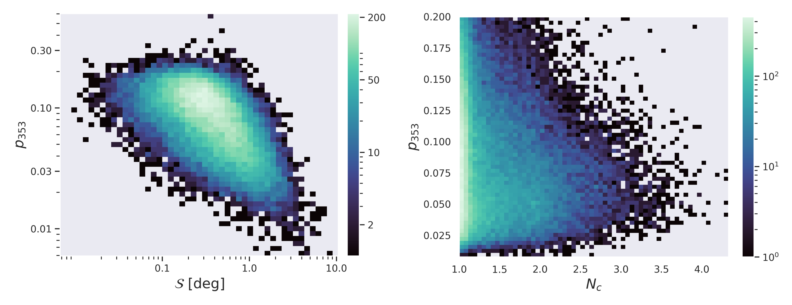
Figure 5: Two-dimensional histograms of $p_{353}$ vs. $\mathcal{S}$ (left) and $p_{353}$ vs. $N_{c}$ (right) in the high Galactic latitude ($|b|>30\degree$) GALFA-H I sky. Regions of high polarization angle dispersion generally correspond to lower polarization fraction, while regions of high LOS complexity correspond to a decrease in the range and the mean value of $p_{353}$.

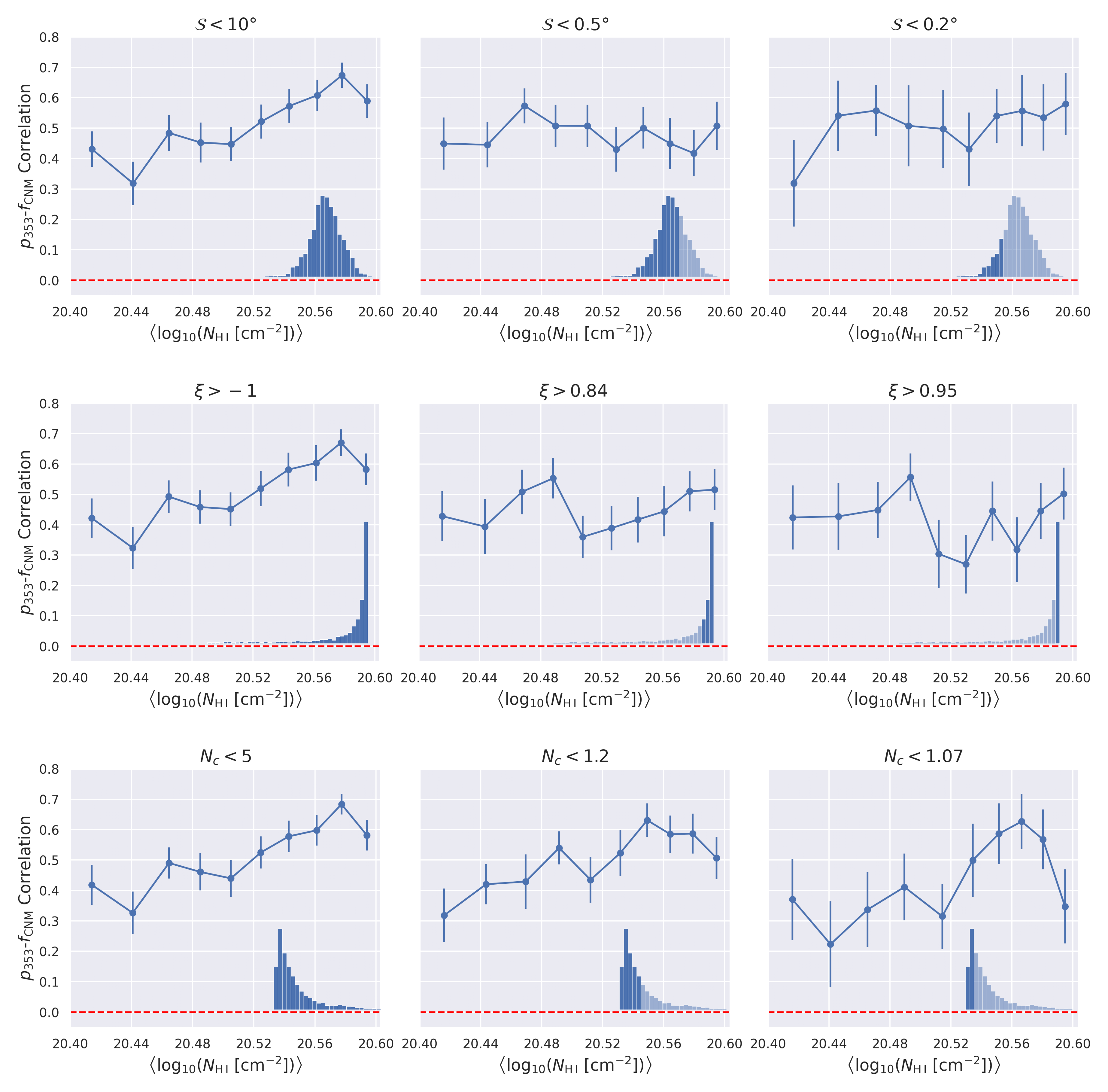
Figure 6: Column-density-binned $p_{353}$-$f_{\mathrm{CNM}}$ correlation over masks defined by different values of the polarization angle dispersion $\mathcal{S}$ (top), degree of alignment between H I and dust polarization angles $\xi$ (middle), and LOS complexity $N_{c}$ (bottom). The distribution of $\mathcal{S}$, $\xi$, $N_{c}$ are shown at the bottom left of each panel. From left to right, the limits are set to represent approximately 100%–60%–20% of the data. The strong $p_{353}$-$f_{\mathrm{CNM}}$ correlation persists across different $\mathcal{S}$, $\xi$, $N_{c}$ value limits.

4.2 Correlation Not Driven By POS Dispersion

One aspect of magnetic field structure that affects polarization fraction is the variation of the inclination angle $\gamma$. As specified in Equations 2–5, $p$ is maximum when the magnetic field is entirely in the POS. In the general case where $\gamma$ is nonzero, the $p$ will be lower than its theoretical maximum, and is zero when the magnetic field is perfectly parallel to the LOS. Inclination angle is also related to the magnetic field angle dispersion in the POS. When the mean magnetic field is nearly parallel to the LOS, small perturbations to the 3D orientation of the magnetic field will result in large changes to its POS projection, resulting in depolarization due to disordered magnetic field orientations along the LOS and within the beam. However, in this study we do not expect these effects to translate into a significant contribution to the $p_{\mathrm{353}}$-$f_{\mathrm{CNM}}$ correlation, since we do not expect $\gamma$ to correlate with $f_{\mathrm{CNM}}$ across large regions of the diffuse sky that are not physically connected. We test that expectation by examining the variation of $p_{\mathrm{353}}$-$f_{\mathrm{CNM}}$ correlation in regions of different degrees of POS polarization angle dispersion.

Magnetic field dispersion in the POS can be characterized by the polarization angle dispersion function:

$$\mathcal{S}(\boldsymbol{r},\delta)=\sqrt{\frac{1}{N}\sum_{i=1}^{N}[\psi(\boldsymbol{r}+\boldsymbol{\delta_{i}})-\psi(\boldsymbol{r})]^{2}}$$ (7)

where $i$ sums over $N$ pixels within an annulus of inner radius $\delta/2$ and outer radius $3\delta/2$. We estimate the dispersion function from the Stokes $Q$ and $U$ parameters, at 80′ resolution with a lag $\delta$=40′ (Planck Collaboration et al., 2020). $\mathcal{S}$ quantifies the local variance of the polarization angle on the POS. In the left panel of Figure 5, we show the distribution of $p_{353}$ vs. $\mathcal{S}$ in the high-latitude GALFA-H I footprint. Consistent with the results from Planck Collaboration et al. (2020), regions of high polarization angle dispersion correspond to lower polarization fraction.

We also make use of another quantity related to polarization angle dispersion discussed in Clark & Hensley (2019). When comparing the H I-based and dust 353 GHz polarization maps, the authors also computed the angular difference between H I and dust polarization angles:

$$\delta\theta=\frac{1}{2}\arctan{\left[\frac{\sin{2\theta_{\mathrm{H\,I}}}\cos{\theta_{353}}-\cos{2\theta_{\mathrm{H\,I}}}\sin{\theta_{353}}}{\cos{2\theta_{\mathrm{H\,I}}}\cos{\theta_{353}}+\sin{2\theta_{\mathrm{H\,I}}}\sin{\theta_{353}}}\right]}$$ (8)

where $\theta_{\mathrm{H\,I}}$ and $\theta_{353}$ are the H I orientation and dust 353 GHz polarization angles respectively. They further define from $\delta\theta$ a measure of the mean degree of alignment:

$$\xi=\left<\cos{2\delta\theta}\right>$$ (9)

so that $\xi=1$ corresponds to perfect alignment, and $\xi=-1$ corresponds to anti-alignment where $\theta_{\mathrm{H\,I}}$ and $\theta_{353}$ are perpendicular to each other. Examining the degree of alignment $\xi$ as a function of H I-based dispersion function $\mathcal{S}$, they found a strong anti-correlation, suggesting that regions of low dispersion where the mean magnetic field is more likely to be in the POS, are also where the measured H I and dust polarization angles are preferentially aligned.

To empirically test whether these effects drive the observed $p_{\mathrm{353}}$-$f_{\mathrm{CNM}}$ relation, we examine if there is a loss of correlation in regions of increasingly narrow $\mathcal{S}$ and $\xi$ ranges. The results are shown in the top and middle panels of Figure 6. The specific limits of $\mathcal{S}$ and $\xi$ are determined so that the panels from left to right account for approximately 100%–60%–20% of the data respectively. The degree of $p_{\mathrm{353}}$-$f_{\mathrm{CNM}}$ correlation is consistent even at low $\mathcal{S}$ and high $\xi$ limits, suggesting that the correlation trend persists when the magnetic field mostly lies on the plane of the sky, and neither $\gamma$ variation nor POS dispersion drives the $p_{353}$-$f_{\rm CNM}$ correlation.

4.3 Correlation Not Driven by LOS H I Components

The presence of multiple dust clouds – traced by multiple H I components – along the LOS can also contribute to the polarization fraction variation. The basic picture is that sightlines dominated by a single H I cloud are more likely to represent a single dust cloud with a coherent ambient mean magnetic field than sightlines with multiple H I clouds, which may in general be separated in distance along the LOS (Pelgrims et al., 2021). Here we examine whether this effect can account for the observed $p_{353}$-$f_{\mathrm{CNM}}$ relation without explicit assumptions about how the magnetic field structure varies across phases. We use the column-density weighted LOS complexity measure $N_{c}$ discussed in Section 2.4 and defined in Equation 1. We show the 2D histogram of $N_{c}$-$p_{353}$ in the right panel of Figure 5. We observe a decrease of the range and mean $p_{353}$ values with increasing LOS complexity $N_{c}$, consistent with what Panopoulou & Lenz (2020) found.

To test if the $p_{353}$-$N_{c}$ relation might drive the observed $p_{353}$-$f_{\mathrm{CNM}}$ correlation, we examine whether there is a loss of $p_{\mathrm{353}}$-$f_{\mathrm{CNM}}$ correlation when we restrict to narrower ranges of $N_{c}$. As the bottom panels of Figure 6 show, similar to the $\mathcal{S}$ and $\xi$ results in Section 4.2, we find that the strong positive $p_{\mathrm{353}}$-$f_{\mathrm{CNM}}$ correlation persists even when limited to a narrow range of $N_{c}$ values, and at low $N_{c}\sim 1$ where the H I emission is dominated by a single H I cloud.

In conclusion, we argued that grain property variation does not play a significant role in the high-latitude diffuse sky, and showed that the relationships between $p_{353}$ and magnetic field properties like inclination angle $\gamma$, POS dispersion $\mathcal{S}$, and LOS complexity $N_{c}$ are not sufficient to produce the observed positive $p_{\mathrm{353}}$-$f_{\mathrm{CNM}}$ correlation. Thus, the correct explanation most likely requires an explicit assumption on the relative disorder of the magnetic field between interstellar volumes occupied by different H I phases. We examine this hypothesis in the next section.

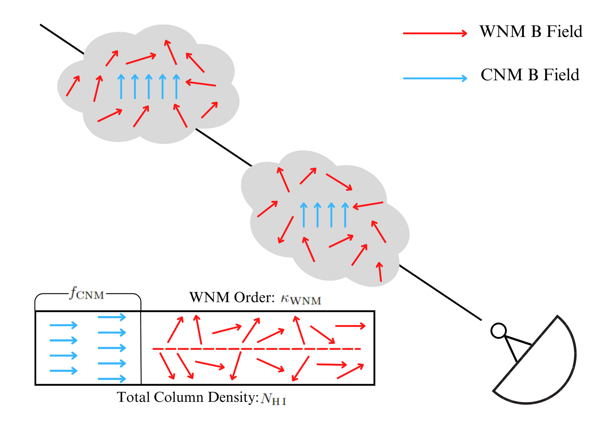
Figure 7: Cartoon illustration of relative disorder of magnetic fields between CNM and WNM as observed along a given line of sight described by model1. If the WNM magnetic field is more disordered than that of the CNM as illustrated in the figure, then sightlines with higher CNM fraction will suffer from less LOS depolarization, resulting in a positive $p_{353}$-$f_{\mathrm{CNM}}$ correlation. In this cartoon, the relative fraction of the column occupied by each phase (bottom rectangle) is representative of the real sky, but the relative fraction of the ISM volume (cartoon clouds) is not.

5 Modeling the Dust Polarization - H I Phase Connection

Having ruled out other factors discussed in Section 4 as drivers of the observed $p_{353}$-$f_{\rm CNM}$ relation, here we argue that the correlation is best reproduced by explicitly modeling LOS magnetic field disorder as dependent on H I phase. This disorder is characterized by the variation of the POS angle $\psi$ in Equations 2 and 3, where a more uniform magnetic field adds constructively when integrated along the LOS, resulting in higher observed $p$. Thus, if there is a difference in the magnetic field disorder between different phases of the ISM, a relationship between $p$ and phase content, like $p_{353}$-$f_{\mathrm{CNM}}$ naturally follows. Specifically, the positive $p_{353}$-$f_{\mathrm{CNM}}$ correlation discussed here could point to a more magnetically ordered CNM compared to more tangled magnetic field structures in the WNM. Because the CNM occupies a much smaller volume than the WNM, a relatively ordered magnetic field structure on CNM length scales is a reasonable starting assumption. In other words, any region of WNM will occupy a much larger path length than a region of equivalent-column-density CNM, and thus will in general experience more variation in the magnetic field orientation. Here, we quantitatively constrain the additional LOS depolarization that is attributable to the WNM-associated dust. First, we present a series of cartoon models that parameterize the separate contributions to the integrated dust polarization signal from the dust associated with the WNM gas and that associated with the CNM gas. For simplicity we will refer to the magnetic fields in these regions as the “CNM magnetic field” and “WNM magnetic field” from now on. Since the $f_{\mathrm{CNM}}$ data we utilize here measures the CNM component as a fraction of the total H I column, here we use WNM to denote anything not captured by the $f_{\mathrm{CNM}}$ measurement, which in general also includes a contribution from the thermally unstable medium.

5.1 Phase-Dependent Cartoon Models

To explicitly model the dependence of the polarization fraction on the variation of the POS component of magnetic fields along the LOS across H I phases, we follow the formalism presented in Equations 2–6. Based on the result of Section 4.2 that $\gamma$ variation does not contribute meaningfully to the $p_{\mathrm{353}}$-$f_{\mathrm{CNM}}$ correlation, we assume without loss of generality that $\gamma=0$. To model varying magnetic field disorder across H I phases, we rewrite Equations 2 and 3 into contributions from separate WNM and CNM components. For simplicity, we further assume uniform volume densities in each phase ($\rho_{\rm CNM}$, $\rho_{\rm WNM}$) to rewrite the equations in terms of CNM and WNM column densities. We denote all model quantities in this setup “model1” to distinguish it from an updated model we will introduce later:

$$Q_{\rm model1} =\sum_{i}^{\mathrm{phase}}\sum_{s}^{\rm LOS}\alpha N_{i}\cos{2\psi_{i}(s)}$$ (10)

$$U_{\rm model1} =\sum_{i}^{\mathrm{phase}}\sum_{s}^{\rm LOS}\alpha N_{i}\sin{2\psi_{i}(s)}$$ (11)

where $i=$ CNM or WNM, and $N_{\rm CNM(WNM)}=f_{\rm CNM(WNM)}N_{\rm H\,I}=\int\rho_{\rm CNM(WNM)}\,ds$ is the CNM (WNM) column density. The model polarization fraction $p_{model1}$ can be computed from $Q_{\rm model1}$, $U_{\rm model1}$ and the total column density $N_{\rm HI}$:

$$p_{\rm model1}=\sqrt{Q_{\rm model1}^{2}+U_{\rm model1}^{2}}/\sum_{i}^{\mathrm{phase}}{N_{i}}$$ (12)

The magnetic field disorder of a given phase is encoded by the variation of $\psi_{i}(s)$ along the LOS. Motivated by the correlation between dust polarization angles and the orientation of primarily-CNM H I filaments, we assume the CNM and the WNM column have the same mean magnetic field orientations, and the relative disorder of the WNM magnetic field is reflected by the dispersion from this aligned mean orientation. We make the simplifying assumption that the CNM magnetic field is maximally ordered (i.e. the magnetic field angle $\psi_{i}$ is the same in all CNM components), so that $p_{\rm max}=p_{\rm CNM}$, and define $\psi_{\mathrm{WNM}}(s)$ to have some degree of disorder relative to the constant $\psi_{\mathrm{CNM}}$ angle. This assumption equates to $p_{\rm model1}=p_{\rm max}=p_{\rm CNM}$ for a column with $f_{\rm CNM}=1$. While physical CNM structures will certainly have some degree of LOS tangling within the CNM path length, the resulting additional depolarization should only affect $p_{\rm max}$ (the upper limit of $p_{\mathrm{model1}}$) but not the $p_{\mathrm{model1}}$-$f_{\mathrm{CNM}}$ correlation. For the WNM magnetic field, we model $\psi_{\mathrm{WNM}}(s)$ using the von Mises distribution, which is the Gaussian distribution analog for circular variables like angles:

$$f(\psi|\mu,\kappa)=\frac{e^{\kappa\cos{(2\psi-\mu)}}}{\pi I_{0}(\kappa)}$$ (13)

where $I_{0}$ is the zeroth order modified Bessel function of the first kind, $\mu$ specifies the mean of the distribution, and $\kappa$ is a measure of concentration ranging from 0 to $\infty$. Here, we set $\mu_{\mathrm{WNM}}=\psi_{\mathrm{CNM}}$, and remap $\kappa$ to [0, 1] by computing the circular variance of the distribution:

$$\kappa^{\prime}=1-\mathrm{Var}(\psi)=\left|\mathbb{E}[e^{i2\psi}]\right|=\frac{I_{1}(\kappa)}{I_{0}(\kappa)}$$ (14)

where $I_{i}$ is the modified Bessel function of order $i$. Henceforth we will simply denote the remapped $\kappa^{\prime}$ as $\kappa$. Equation 14 is effectively the degree of depolarization due to magnetic field tangling in a column that is entirely WNM ($f_{\rm CNM}=0$). It follows that $\kappa$ is equivalent to $p_{\rm WNM}/p_{\rm max}$, where $\kappa=0$ corresponds to a uniform $\psi_{\rm WNM}(s)$ distribution over $[-\pi/2,\pi/2]$ and $p_{\rm WNM}=0$, and $\kappa=1$ corresponds to $\psi_{\rm WNM}(s)=\psi_{\rm CNM}$ and $p_{\rm WNM}=p_{\rm max}$.

Therefore, model1, as defined by Equations 10–14, is a two parameter model ($p_{\rm max}$, $\kappa_{\mathrm{WNM}}$) that effectively constrains the polarization fraction in the magnetically-ordered CNM column $p_{\rm CNM}=p_{\rm max}$, and the relative degree of depolarization due to magnetic field tangling in the WNM vs. the CNM, $p_{\rm WNM}/p_{\rm CNM}$. Equations 10–14 can be condensed into a linear model of $p$:

$$p_{\rm model1} =f_{\rm CNM}\cdot p_{\rm CNM}+(1-f_{\rm CNM})\cdot p_{\rm WNM}$$ (15)

$$=p_{\rm max}\bigl{(}f_{\rm CNM}+(1-f_{\rm CNM})\kappa\bigr{)}$$

$$=p_{\rm max}(1-\kappa)f_{\rm CNM}+p_{\rm max}\kappa$$

Fitting the model to the observed $p_{353}$-$f_{\rm CNM}$ data is equivalent to deriving a best-fit linear relation, where the slope is parameterized by $p_{\rm max}(1-\kappa)$, and the intercept by $p_{\rm max}\kappa$. We illustrate the setup of this simple cartoon model in Figure 7.

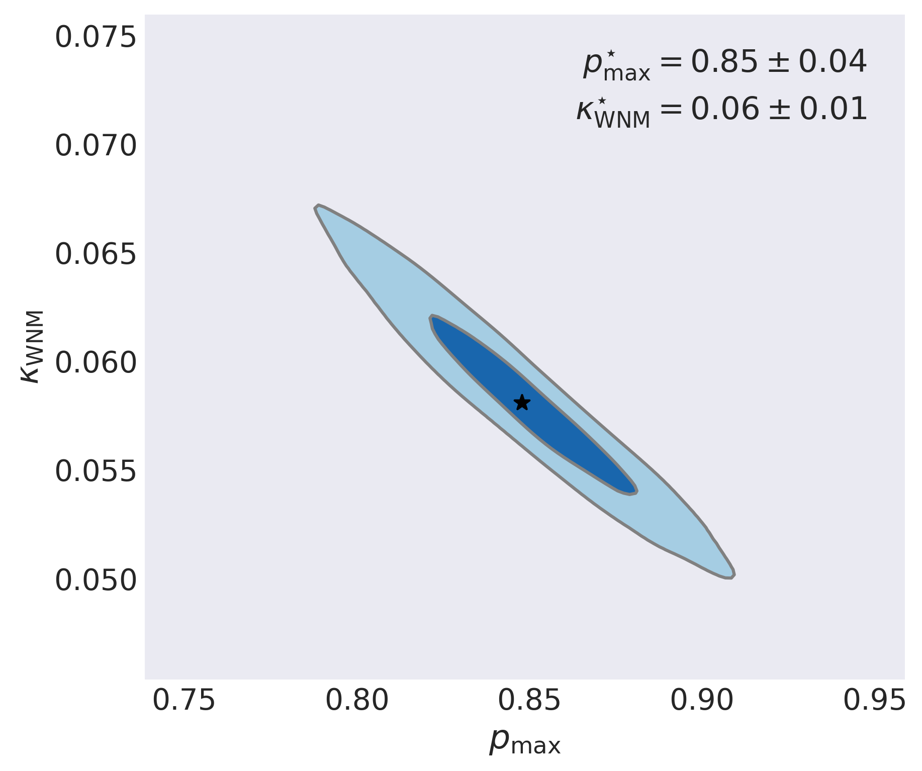
Figure 8: Posterior distribution of maximum intrinsic polarization fraction $p_{\mathrm{max}}$ and WNM order parameter $\kappa_{\mathrm{WNM}}$, after fitting the cartoon polarization model described in Figure 7 to $p_{353}$-$f_{\mathrm{CNM}}$ data. The results show that explaining the observed strong $p_{353}$-$f_{\mathrm{CNM}}$ correlation with a simple model of phase depolarization due to a single disordered WNM component relative to an ordered CNM component requires the intrinsic dust polarization to be unphysically large.

5.2 Phase-Dependent Magnetic Field Interpretation

We examine the result of fitting model1 to the observed $p_{353}$ and $f_{\rm CNM}$ data by applying Bayesian hierarchical linear regression. We model the likelihood of the data as

$$\mathcal{L} =P(f_{\rm CNM},p_{353}|\hat{f}_{\rm CNM},\hat{p}_{353})P(\hat{p}_{353}|\hat{f}_{\rm CNM},\mathbf{\theta})$$ (16)

where $\hat{p}_{353}$ and $\hat{f}_{\rm CNM}$ are the true, unobserved values of the polarization fraction and CNM fraction, respectively, and $\mathbf{\theta}=(\kappa,p_{\rm max},\sigma_{p}^{2})$ are the parameters of our model. Then

$$P(\hat{p}_{353}|\hat{f}_{\rm CNM},\mathbf{\theta})\sim\mathcal{N}({\rm model(\hat{f}_{\rm CNM},\theta)},\sigma_{p}^{2})$$ (17)

$$P(p_{353}|\hat{p}_{353})\sim\mathcal{N}(\hat{p}_{353},\sigma^{2}_{\hat{p}_{353}})$$ (18)

$$P(f_{\rm CNM}|\hat{f}_{\rm CNM})\sim\mathcal{N}(\hat{f}_{\rm CNM},\sigma^{2}_{\hat{f}_{\rm CNM}})$$ (19)

where $\rm model(\hat{f}_{CNM},\theta)$ is given by Equation 15.

We assume a uniform prior distribution for $p_{\rm max}$ and $\kappa_{\mathrm{WNM}}$ over [0, 1]. For $\sigma_{p}$, we follow the convention of using a half-Cauchy distribution as the uninformative prior for global variance parameters in Bayesian models (Polson & Scott, 2011). Physically, $\sigma_{p}$ models the additional variance in $p_{353}$ that is uncorrelated with $f_{\rm CNM}$ and thus not captured by model1, e.g. POS dispersion due to inclination angle variation. In Section 4, we argued that polarization fraction variation is affected by different factors of grain properties and magnetic field geometry, but the observed $p_{353}$-$f_{\rm CNM}$ relation cannot be explained without an explicit phase-dependent assumption. Here we use model1 to capture the phase-dependent $p$ variation due to relative magnetic field disorder across phases, and encapsulate other sources of $p_{353}$ variance into a global variance parameter $\sigma_{p}$.

Performing the Bayesian regression fit with PyMC, we apply Markov Chain Monte Carlo (MCMC) to sample the posterior distribution and show the results for model1 parameters in Figure 8. The $1\sigma$ best-fit values are $(p_{\rm max}=0.85\pm 0.04,\kappa_{\rm WNM}=0.06\pm 0.01,\sigma_{p}=0.036\pm 0.001)$. This corresponds to a best-fit slope of 0.80 and intercept of 0.05 for the linear model specified in Equation 15. The relatively small $\sigma_{p}$ value and $\kappa_{\rm WNM}<1$ are consistent with the discussions in Section 4 that the observed $p_{353}$-$f_{\mathrm{CNM}}$ relation cannot be explained without explicit assumption on phase-dependent magnetic field structure variations. $\kappa_{\rm WNM}=0.058$ corresponds to $p_{\rm WNM}=5.8\%$ of $p_{\rm max}$ and therefore highly depolarizing WNM magnetic fields relative to the CNM magnetic fields. However, the best-fit $p_{\rm max}$ value is significantly higher than the observed max $p_{353}\sim 0.22$ and far exceeds the maximum intrinsic polarization fractions derived from typical dust grain models (Kirchschlager et al., 2019; Draine & Hensley, 2021). This means that the current model cannot fully explain the observed $p_{353}$-$f_{\mathrm{CNM}}$ correlation. Specifically, the model cannot consistently account for both the high slope in the $p_{353}$-$f_{\rm CNM}$ relation and the maximum observed $p_{353}$ value without an unphysically high $p_{\rm max}$. According to Equation 15, the $p$-$f_{\rm CNM}$ slope is $p_{\rm max}(1-\kappa)$. The steep observed $p_{353}$-$f_{\rm CNM}$ slope is such that $p_{\rm max}$ needs to be large, and $\kappa$ and thus $p_{\rm WNM}/p_{\rm CNM}$ must be close to zero. Small $\kappa$ means the WNM column is almost entirely depolarizing. Thus, for the LOS-averaged $p_{\rm model1}$ to match the range of maximum observed $p_{353}\sim 0.22$ despite the significant depolarization in the WNM fraction, the small CNM fraction must be highly polarized to make up the difference, leading to the unphysically large $p_{\rm max}=p_{\rm CNM}=0.85\pm 0.04$ fit result in model1. On the other hand, if we force $p_{\rm max}=0.22$ with other parameters being the same as the model1 best-fit values, then the resulting $p_{\rm model}$ will only have a 90th percentile value of 0.08, half of the observed 90th-percentile $p_{353}$ value of 0.16. If we instead fit model1 but fix $p_{\rm max}=0.22$, we get best-fit parameters $\kappa_{\rm WNM}=0.39\pm 0.01,\sigma_{p}=0.043\pm 0.001)$. The higher $\sigma_{p}$ value means that more of the $p_{353}$ scatter is attributed factors uncorrelated with $f_{\rm CNM}$, and the resulting $p_{\rm model}$-$f_{\rm CNM}$ relation has a Spearman coefficient of 0.11, much less than 0.50 for the observed $p_{353}$-$f_{\rm CNM}$ correlation. Thus, the observed $p_{353}$-$f_{\rm CNM}$ slope and maximum $p_{353}$ are such that model1 cannot fit the data without an unphysically high $p_{\rm max}$ value. Thus, there must be some additional contribution to the observed $p_{353}$-$f_{\mathrm{CNM}}$ relationship that is not explained by this simple model of WNM magnetic field tangling relative to an ordered CNM.

One possible contribution is increased dust emissivity in the CNM. So far, we have implicitly assumed that the dust emissivity is the same between CNM-associated dust and WNM-associated dust. While phase-dependent dust emissivity does not by itself result in a $p_{353}$-$f_{\mathrm{CNM}}$ relation, if the dust associated with the CNM has a higher emissivity, it will have a higher weight in the LOS average. If the CNM-associated dust also experiences a more ordered magnetic field, this will result in a larger polarization fraction when averaged over the whole column than a simple model where the CNM and WNM components are weighted only by their respective column densities. The result is higher $p$ at the same degree of $f_{\rm CNM}$ compared to when CNM and WNM emissivity are weighted equally, leading to a higher $p_{353}$-$f_{\mathrm{CNM}}$ slope and alleviating the tension discussed with model1. Past work has found a consistent increase of the FIR emission over H I column density ratio $I_{857}/N_{\rm H\,I}$ toward sightlines with more CNM (Clark et al., 2019; Murray et al., 2020; Lei & Clark, 2023). However, since in this study we are restricting to diffuse regions where the variation in the dust to H I emission ratio is less than 10% (Lenz et al., 2017), we do not expect a significant contribution from this effect. For the column density regime ($N_{\mathrm{H\,I}}<4\times 10^{20}~{}\mathrm{cm^{-2}}$) and scale (80′) considered in this study, we find that there is only a small $I_{857}/N_{\rm H\,I}$ ratio variation with increasing $f_{\rm CNM}$, consistent with a 10% scatter. Instead, we reexamine our magnetic field disorder assumptions.

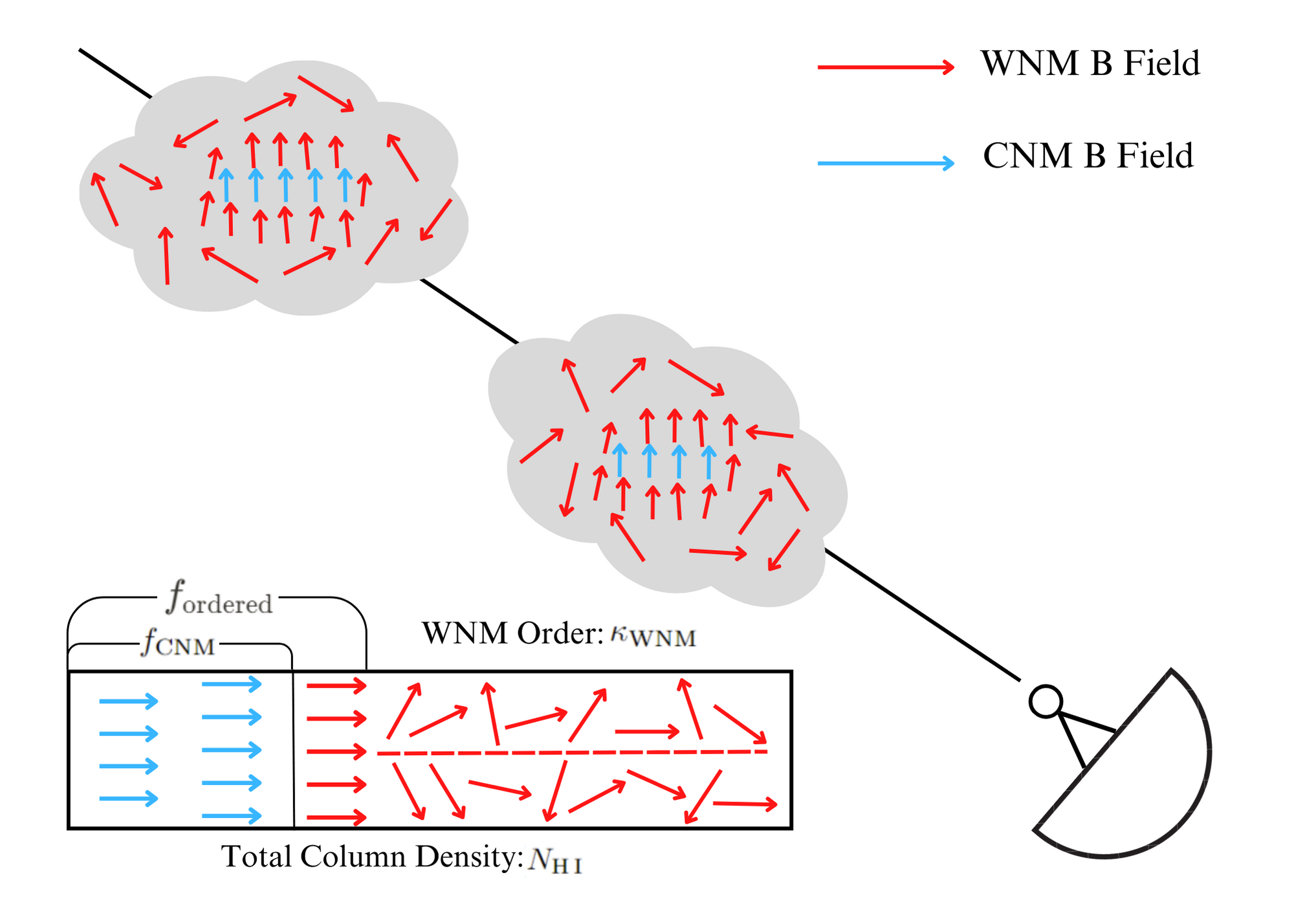
Figure 9: Cartoon illustration of the relative disorder of magnetic fields between CNM and WNM as observed along a given line of sight described by model2. Compared to Figure 7, we allow for a factor that parameterizes a fraction of the CNM-neighboring WNM region that also has more ordered magnetic field orientations.

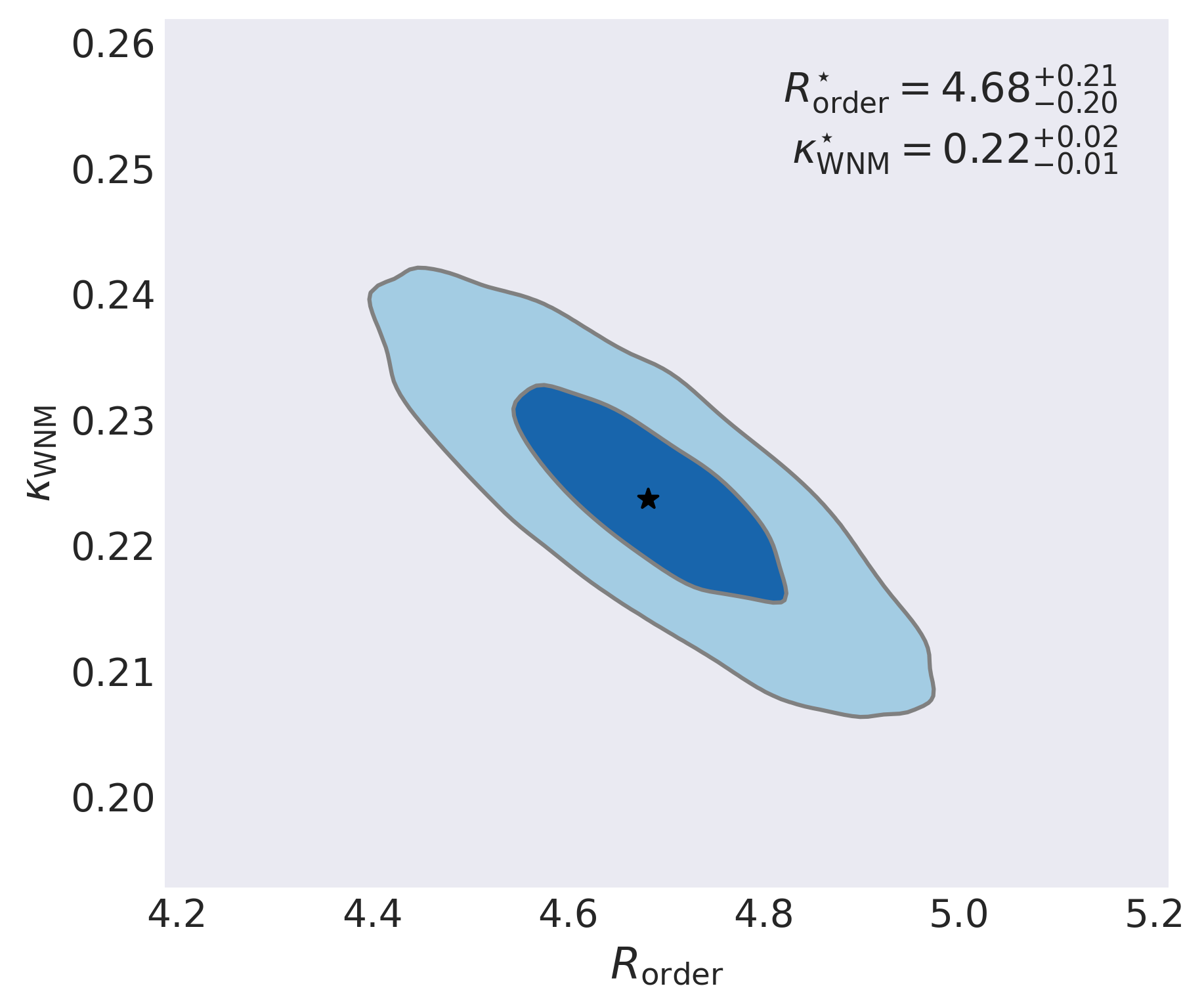
Figure 10: Posterior distribution of WNM order parameter $\kappa_{\mathrm{WNM}}$, and ratio of ordered component fraction to CNM fraction $R_{\mathrm{ordered}}=f_{\mathrm{ordered}}/f_{\mathrm{CNM}}$, after fitting model2 to $p_{353}$-$f_{\mathrm{CNM}}$ data. The $1\sigma$ best-fit parameter values are $(R_{\rm order}=4.68^{+0.21}_{-0.20},\kappa_{\rm WNM}=0.22^{+0.02}_{-0.01})$.

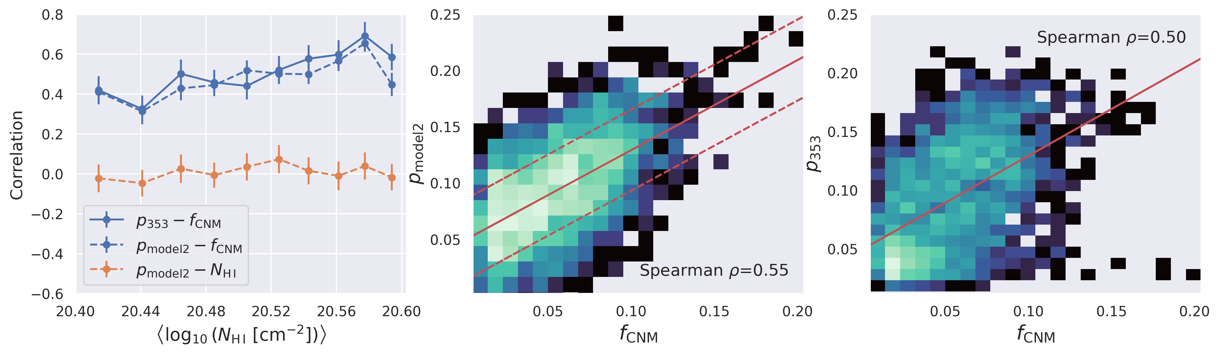
Figure 11: Left: Column-density-binned correlation of $f_{\mathrm{CNM}}$ and $N_{\mathrm{H\,I}}$ with model polarization fraction $p_{\mathrm{model2}}$ computed with best-fit parameters ($R_{\mathrm{ordered}}=4.68$, $\kappa_{\mathrm{WNM}}=0.22$, $\sigma_{p}=0.036$). Middle: 2D histogram of $p_{\mathrm{model2}}$-$f_{\rm CNM}$, with the solid red line indicating the best-fit mean $p_{\mathrm{model2}}$ and the dashed red lines the $\sigma_{p}$ scatter in Equation 17. Right: The same best-fit linear relation overlaid on the observed $p_{353}$-$f_{\rm CNM}$ 2D histogram. The positive $p_{\rm model2}$-$f_{\rm CNM}$ correlation is consistent with the observed $p_{353}$-$f_{\rm CNM}$ correlation, while $p_{\rm model2}$-$N_{\rm HI}$ is consistent with no correlation.

In the cartoon model illustrated in Figure 7, we assumed that along each sightline there is a single parameter $\kappa_{\mathrm{WNM}}$ characterizing the tangling of the WNM (i.e., the non-CNM) magnetic field relative to that of the CNM. In general, in the canonical picture of a thermally bistable H I gas, the CNM condenses out of the diffuse WNM driven by turbulence and thermal instability (Wolfire et al., 2003; Saury et al., 2014). If the WNM magnetic field is more disordered to begin with, and a more ordered CNM magnetic field forms out of the compression and condensation process, then we might naturally expect the gas that neighbors the sites of CNM formation and the thermally unstable medium to have intermediate degrees of magnetic field disorder as well. We could further hypothesize that the fraction of this “ordered WNM” region associated with CNM formation would correlate with $f_{\mathrm{CNM}}$. This would enhance the effect of a more ordered CNM magnetic field adding constructively to higher observed $p$, resulting in a stronger $p_{353}$-$f_{\mathrm{CNM}}$ correlation. This scenario is illustrated in the updated cartoon model shown in Figure 9. We denote the updated model “model2” in contrast to model1 presented in Figure 7.

Here, in the spirit of the cartoon model, instead of trying to model the exact distribution of this variation, we define $f_{\mathrm{ordered}}$ to parameterize the total fraction of magnetically ordered regions including both the CNM and the fraction of the WNM column we assume to be ordered. To encode that the additional ordered component should correlate with $f_{\mathrm{CNM}}$, we define $R_{\mathrm{ordered}}$ as a ratio of $f_{\mathrm{ordered}}$ and $f_{\mathrm{CNM}}$:

$$R_{\mathrm{ordered}}=f_{\mathrm{ordered}}/f_{\mathrm{CNM}}.$$ (20)

We emphasize that the fact that $f_{\mathrm{ordered}}$ is proportional to $f_{\mathrm{CNM}}$ means that this model is not degenerate with simply raising $\kappa$ in model1. Instead, $R_{\mathrm{ordered}}$ serves as an additional weighting factor to the slope of the $p_{533}-f_{\rm CNM}$ relation. We introduce $R_{\mathrm{ordered}}$ as a new parameter in model2. Furthermore, instead of fitting $p_{\rm max}$ as a free variable, we fix it to a physically motivated value. As a result, model2 is a re-parameterization of the linear model of the $p_{533}-f_{\rm CNM}$ relation from ($p_{\rm max}$, $\kappa_{\rm WNM}$) in model1 to ($R_{\mathrm{ordered}}$, $\kappa_{\rm WNM}$), and Equation 15 becomes:

$$p_{\rm model2} =f_{\mathrm{ordered}}\cdot p_{\rm max}+(1-f_{\mathrm{ordered}})\cdot p_{\rm WNM}$$ (21)

$$=p_{\rm max}\bigl{(}Rf_{\rm CNM}+(1-Rf_{\rm CNM})\kappa\bigr{)}$$

$$=p_{\rm max}R(1-\kappa)f_{\rm CNM}+p_{\rm max}\kappa$$

We fix $p_{\rm max}$ according to the maximum observed $p^{\rm max}_{353}=22^{+3.5}_{-1.4}\%$ as determined by Planck full-sky observations at 353 GHz and $80\arcmin$ resolution (Planck Collaboration et al., 2020). The state-of-the-art model of interstellar dust grains known as Astrodust (Hensley & Draine, 2022) gives a similar constraint at $p_{\rm max}\sim 19.2\%$ at 353 GHz. The uncertainty on $p^{\rm max}_{353}$ is dominated by uncertainty on the total intensity zero level. Here we present the result for setting $p^{\rm max}_{353}=22\%$, assuming the fiducial Galactic emission offset of 40 $\mu\mathrm{K_{CMB}}$ Planck Collaboration et al. (2020). We also repeat the same analysis using the upper and lower limits for this offset.

Performing the Bayesian regression fit process described by Equations 16-17 for model2, replacing the Equation 15 parameterization of the linear relation with Equation 21, we show the resulting posterior distributions of model2 parameters in Figure 10. Since we are still performing the same linear model fit just with the slope and intercept reparametrized, the (slope, intercept, $\sigma_{p}$) has the same best-fit values of (0.80, 0.05, 0.036) as in model1. The $1\sigma$ best-fit values of the model2 parameters are $(R_{\rm order}=4.68^{+0.21}_{-0.20},\kappa_{\rm WNM}=0.22^{+0.02}_{-0.01})$. In the diffuse regions we are considering, the CNM accounts for $\sim 5\%$ of the total H I mass (Murray et al., 2020). Thus, $R_{\mathrm{ordered}}=4.68$ would imply that the magnetically ordered fraction of the WNM column accounts for an additional $\sim 18.4\%$ of the H I mass. Using the best-fit ($R_{\mathrm{ordered}}=4.68$, $\kappa_{\mathrm{WNM}}=0.22$, $\sigma_{p}=0.036$) parameters with $p_{\rm max}=0.22$, we make a random realization of $p_{model2}$ using Equations 17 and 21 and show its correlation relations with observed data in Figure 11. $R_{\mathrm{ordered}}$ and $\kappa_{\mathrm{WNM}}$ determine the best-fit mean $p_{model2}$ line shown in red, while the scatter in $p_{model2}$ is due entirely to $\sigma_{p}$. We verify that the degree of $p_{\rm model2}$-$f_{\rm CNM}$ correlation is consistent with the observed $p_{353}$-$f_{\rm CNM}$ behavior, while $p_{\rm model2}$-$N_{\rm HI}$ is compatible with no correlation. These results show that the cartoon model of magnetic field structure variation across phases illustrated in Figure 9 is compatible with the observed $p_{353}-f_{\mathrm{CNM}}$ correlation.

We repeat the modeling fitting procedure while adopting the high vs. low Galactic offset limit to explore the effect of total intensity zero-level uncertainty on the fitting results. Following Planck Collaboration et al. (2020), we apply a low offset of 23 $\mu\mathrm{K_{CMB}}$ with $p^{\rm max}_{353}=25.5\%$, and a high offset of 103 $\mu\mathrm{K_{CMB}}$ with $p^{\rm max}_{353}=20.6\%$. The best-fit values are $(R_{\rm order}=4.13^{+0.20}_{-0.21},\kappa_{\rm WNM}=0.22^{+0.02}_{-0.01})$ and $(R_{\rm order}=4.74^{+0.19}_{-0.20},\kappa_{\rm WNM}=0.21^{+0.02}_{-0.01})$ for the low and high offset respectively, consistent with the fit with fiducial offset values to within $\sim 12\%$. Note that best-fit $R_{\rm order}$ increases more significantly with decreased fixed $p_{\rm max}$ value while $\kappa_{\rm WNM}$ barely changes. Thus in this model, a lower polarization fraction in the CNM, which may be more easily explained by physical dust models, requires a larger $f_{\rm CNM}$-correlated dust column to be polarized at the same level.

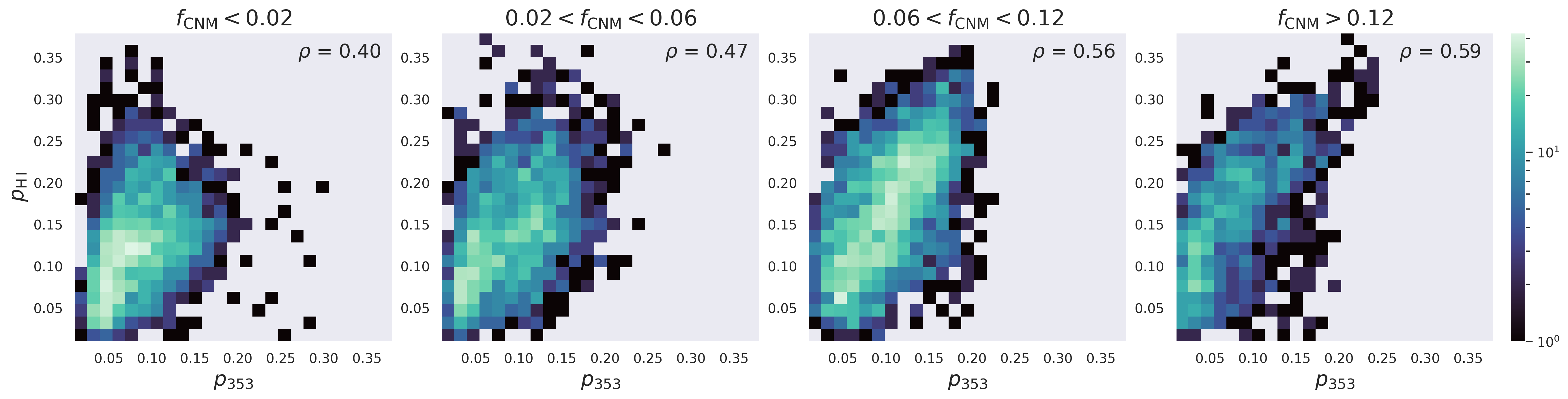
Figure 12: Two-dimensional histograms of $p_{353}$ and $p_{\mathrm{H\,I}}$ in bins of $f_{\mathrm{CNM}}$. The $p_{353}$-$p_{\mathrm{H\,I}}$ correlation increases with increasing $f_{\mathrm{CNM}}$, suggesting that the H I polarization template traces the dust polarization fraction better at higher CNM fraction.

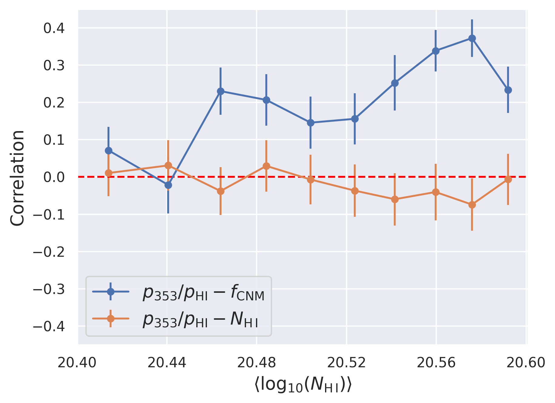
Figure 13: Column-density-binned correlation of polarization fraction ratio $p_{353}/p_{\mathrm{H\,I}}$ with $f_{\mathrm{CNM}}$ and $N_{\mathrm{H\,I}}$. There is a significant positive $p_{353}/p_{\mathrm{H\,I}}$-$f_{\mathrm{CNM}}$ correlation while correlation with $N_{\mathrm{H\,I}}$ is compatible with 0. This is consistent with the interpretation that the $p_{353}$-$p_{\mathrm{H\,I}}$ difference can be partly attributed to the H I polarization template overweighting a more ordered CNM component and underweighting WNM tangling. The agreement improves with increasing CNM fraction and $p_{353}$ increases relative to $p_{\mathrm{H\,I}}$ as WNM tangling plays a lesser role.

5.3 Consistency with H I Polarization Template

As described in Section 2.5, using the orientation of filamentary structures that trace local magnetic fields, Clark & Hensley (2019) constructed 3D (position-position-velocity) Stokes polarization parameter maps from H I intensity data. The H I-based $Q$ and $U$ maps integrated over LOS velocity are found to be well-correlated with the 353 GHz dust $Q$ and $U$ maps. However, since the H I-based polarization templates are constructed from preferentially CNM structures (Kalberla & Haud, 2018; Clark et al., 2019; Peek & Clark, 2019; Murray et al., 2020), we expect them to overweight the contribution of the CNM to the total polarized emission. We examine the variation of the correlation between the H I-based and 353 GHz dust map in regions binned by $f_{\mathrm{CNM}}$ values, to test the consistency of the phase-dependent magnetic field variation interpretation discussed in the previous section.

Clark & Hensley (2019) find that the H I-based polarization fraction $p_{\mathrm{H\,I}}$ is well-correlated with $p_{353}$ (see also Clark, 2018). However, if the H I polarization template over-weights CNM structures, and if there is a difference in CNM and WNM magnetic field disorder, we should expect the $p_{\mathrm{H\,I}}$-$p_{353}$ correlation to be stronger in regions with higher CNM content. In Figure 12, we plot the distribution of $p_{\mathrm{H\,I}}$ vs. $p_{353}$ in regions of increasing $f_{\mathrm{CNM}}$, and find a modest but consistent trend of stronger correlation with increasing CNM fraction. The Spearman correlation coefficient improved from $\rho=0.40$ at $f_{\mathrm{CNM}}<0.02$ to $\rho=0.59$ at $f_{\mathrm{CNM}}>0.12$. The qualitative behavior of this correlation trend is insensitive to the choices of $f_{\mathrm{CNM}}$ range. Furthermore, if the WNM magnetic field orientation is more disordered relative to that of the CNM as proposed in the previous section, by over-weighting a more ordered CNM, $p_{\mathrm{H\,I}}$ should in general overestimate $p_{353}$ in low $f_{\mathrm{CNM}}$ regions relative to high $f_{\mathrm{CNM}}$ regions. This should translate to a positive correlation between the $p_{353}$/$p_{\mathrm{H\,I}}$ ratio and $f_{\mathrm{CNM}}$. In Figure 13, we compute the $p_{353}$/$p_{\mathrm{H\,I}}$-$f_{\mathrm{CNM}}$ correlation in the same equal-area column density bins used for $p_{353}$-$f_{\mathrm{CNM}}$ correlation in Figure 4. We observe a consistent positive correlation as expected for the physical picture we put forward in model2 over most of the column density range, except in the two lowest column density bins. Therefore, the results in Figures 12 and 13 together are consistent with a phase-dependent magnetic field variation interpretation where the magnetic field in the WNM is disordered relative to that of the CNM, resulting in a positive correlation of polarization fraction with CNM content.

6 Discussion

6.1 Interpretations of Phase-Dependent Magnetic Field Properties

The results presented in Sections 4 and 5 show that a difference in magnetic field tangling between the WNM and the CNM is the most likely explanation for the observed positive $p_{\mathrm{353}}$-$f_{\mathrm{CNM}}$ correlation. Thus the results presented here constitute a new constraint on the relationship between multi-phase ISM structure and the magnetic field. Our work complements investigations of magnetic field alignment between ionized and neutral phases, which have mostly focused on small patches of the sky where a direct morphological connection between different tracers is found (Zaroubi et al., 2015; Jelić et al., 2018; Bracco et al., 2020; Campbell et al., 2022). Here we present the first study constraining the relative disorder of the magnetic field between neutral phases of the ISM over large regions of the sky, using statistics of the dust polarization fraction and phase-decomposed maps of H I emission. With the development of ever-more sophisticated phase decomposition techniques (Marchal et al., 2019; Riener et al., 2020; Murray et al., 2020), alongside the increasing availability of H I absorption sightlines from future and ongoing surveys (Dickey et al., 2013; McClure-Griffiths et al., 2015), there are growing opportunities to further test this picture to examine the important question of magnetic field alignment between phases in different environments across different scales.

The data-driven cartoon dust emission model presented in 5.2 allows us to quantitatively constrain the properties of the CNM and the WNM magnetic field. The model parameter posterior distributions in Figure 10 suggest that a CNM with more aligned magnetic fields forms out of the WNM with generally disordered fields. In particular, the best-fit value $\kappa_{\mathrm{WNM}}\sim 0.22$ describes the degree of fractional depolarization due to magnetic field tangling in the WNM column relative to the CNM column. How should we interpret this different degree of geometrical depolarization in terms of the 3D magnetic field structure in each phase? The difference in magnetic field disorder in the WNM and CNM could arise from two main physical pictures. On the one hand, a single statistical distribution of magnetic field structure could exist independent of H I phase, but the magnetic field in the CNM column could be more ordered because the CNM is confined to a much smaller path length and thus samples the distribution only at that smaller scale. The typical CNM path length is $\sim$pc scale, while the WNM is more volume filling with a typical path length of 100 pc or more (Heiles & Troland, 2003; Kalberla & Kerp, 2009). In this case, our measurement of the difference in CNM and WNM magnetic field disorder constrains the overall LOS magnetic field tangling over the WNM scale vs. the CNM scale, and could be used to constrain the scale dependence of the 3D magnetic field structure in the neutral medium.

On the other hand, the difference in magnetic field disorder between the CNM and the WNM could point to distinct magnetic field distributions between the phases. Specifically, the CNM could have a more ordered magnetic field distribution as a result of CNM formation. We argue that the observational constraints presented in this study favor this interpretation oversampling the same magnetic field distribution over different scales. First, the correlation between dust polarization angle and H I CNM filaments implies that in the diffuse ISM, the mean magnetic field orientation in the CNM is well-aligned with the mean magnetic field orientation in the WNM. The correlation between $p_{353}$ and $f_{\rm CNM}$ then constrains the relative dispersion of the WNM magnetic field from the mean orientation. As the middle panels of Figure 6 show, a strong degree of $p_{353}$-$f_{\rm CNM}$ correlation persists in regions with almost perfect $\theta_{H\,I}$-$\theta_{353}$ alignment ($\xi>0.95)$ on the 80′ scales considered in this work. If we argued that the scale-dependence alone were responsible for the different magnetic field dispersion attributed to the CNM and the WNM, we would need to consider the plausibility of a magnetic field geometry that has the WNM-measured dispersion over $\sim 100$ pc scales, but which on any given $\sim$pc-scale region would appear both ordered and aligned with the WNM mean magnetic field orientation. Future work should further explore the different interpretations through detailed study of the magnetic field distribution in CNM formation simulations (Inoue & Inutsuka, 2016; Kim & Ostriker, 2017; Gazol & Villagran, 2021; Moseley et al., 2021; Fielding et al., 2023).

A further constraint is the large best-fit value of $R_{\rm ordered}\sim 4.68$, indicating that a significant portion of the non-CNM column also has a relatively ordered magnetic field. If the additional ordered column spans a significant path length, then the tension between the mean-field constraint and the relative dispersion constraint described above becomes even more severe. Thus the combination of the CNM and this additional ordered component of the column is likely to have a statistically more ordered 3D magnetic field distribution than the disordered WNM column. For the diffuse region considered in this study, $R_{\rm ordered}\sim 4.68$ translates to an average H I mass fraction of $\sim 18.4\%$ for the additional ordered non-CNM column. A natural physical origin for this additional column could be the UNM. Utilizing absorption measurements from the 21-SPONGE survey, (Murray et al., 2018) found the UNM mass fraction to be generally consistent with $\sim 20\%$ of total H I mass (Murray et al., 2018), with the caveat that the region surveyed was not necessarily representative of the diffuse sky we are considering. Ongoing and future H I absorption surveys will add to available data at high latitudes and better constrain properties of the UNM in these regions (Dickey et al., 2013; McClure-Griffiths et al., 2015; Dickey et al., 2022). If the additional magnetically ordered column is UNM, assuming the UNM has a density between the fiducial WNM and CNM densities $[\rho_{\rm CNM}=0.6{\rm\,cm^{-3}},\rho_{\rm WNM}=30{\rm\,cm^{-3}}]$ (Draine, 2011), then the ordered column on average spans a path length between [1pc, 40pc], further adding to the tension between the mean-field constraint and the relative dispersion constraint that any model without an explicitly phase-dependent magnetic field structure needs to explain.

An alternative to interpreting $R_{\rm ordered}$ as the additional magnetically ordered column is the possible role of dust emissivity variation. Higher emissivity in the magnetically ordered regions would lead to higher weighting for the ordered components in the LOS average. Since we modeled $R_{\mathrm{ordered}}$ as a ratio $f_{\rm ordered}/f_{\rm CNM}$, $R_{\mathrm{ordered}}$ effectively serves as an additional weighting term to the CNM contribution in Equations 10 and 11, degenerate with the effect of a higher dust emissivity weighting. Hence, assuming CNM emissivity $\epsilon_{\rm CNM}$ $\geq$ WNM emissivity $\epsilon_{\rm WNM}$, we should consider $f_{\mathrm{ordered}}\sim 4.68f_{\rm CNM}$ as an upper limit on the fraction of magnetically-ordered WNM column. However, we do not consider emissivity variation a significant effect in this study because of the small variation ($\sim$10%) of the dust emission to H I column ratio in the diffuse sky (Lenz et al., 2017). A significant source of the scatter in that relationship in these regions is the photometric uncertainties. However, even if the scatter is caused entirely by higher emissivity in the CNM, in the range of $f_{\rm CNM}\sim(0,0.2)$ considered in our study, a  10% scatter in the dust emission to H I column ratio would only correspond to an emissivity ratio $R=\epsilon_{\rm CNM}/\epsilon_{\rm WNM}\sim 1.5$ relative to the WNM, outside the $2\sigma$ best-fit range we found for $R_{\rm ordered}$.

In summary, the observational constraints presented in this study are most consistent with a higher degree of magnetic field orientation dispersion in the WNM than in the CNM. Numerical simulation studies of CNM formation have mostly focused on the physical and morphological properties of the CNM magnetic field, such as the alignment of magnetic field orientation with cold filaments (Inoue & Inutsuka, 2016; Gazol & Villagran, 2021). Our results on the relative disorder of the magnetic field between the CNM and the WNM columns place a new constraint on CNM formation models that can be directly compared against MHD simulations.

6.2 Implications for Dust Grain Models

The level of maximum observed polarization fraction $p^{\rm max}_{353}\sim 20\%$ found by Planck observations (Planck Collaboration et al., 2015a, 2020) are challenging to reproduce for dust models (Draine & Fraisse, 2009; Guillet et al., 2018; Hensley & Draine, 2021). Characterizing optical starlight polarization in regions of maximally polarized dust emission, Panopoulou et al. (2019) find that the high polarization fractions are unlikely to result from dust properties such as enhanced grain alignment. Instead, they argue that a favorable magnetic field geometry is the most likely explanation, where in the regions of maximum polarization, the magnetic field is mostly in the plane of sky and uniform along the line-of-sight. Here we argue that our results regarding magnetic field disorder between neutral phases, added to the favorable magnetic field geometry argument, potentially make it easier to reconcile the high maximum polarization observation with dust models.

Any sightline will suffer from some degree of geometric depolarization both along the line of sight and within the beam. This is certainly the case at the resolution of the Planck dust maps of 80′ beam size over typical WNM path lengths of over $\sim 100$pc. But if the CNM column is more magnetically ordered than the WNM column, and high polarization fraction regions are associated more with high CNM content which contributes much more significantly to the LOS-averaged $p$ value than the WNM column, then the relevant scale for the favorable magnetic field geometry argument will be the much smaller CNM path length scale $\sim 1$pc. It is more reasonable to expect minimal geometric depolarization over the small and more magnetically ordered CNM columns, strengthening the explanation that favorable magnetic field geometry brings the observed maximum polarization fraction closer to the theoretical maximum.

6.3 Column-Density-Dependent Correlation Behavior

In this study, we focus on exploring interpretations for the positive $p_{\mathrm{353}}$-$f_{\mathrm{CNM}}$ correlation in the most diffuse regions of the sky. As Figures 1 and 2 show, the full $p_{\mathrm{353}}$-$f_{\mathrm{CNM}}$ relation transitions from positive correlation to anticorrelation at higher column densities ($N_{\mathrm{H\,I}}\sim 10^{21}\ \mathrm{cm^{-2}}$). The explanation for this transition, and whether the phase-dependent magnetic field variation interpretation is consistent with the anticorrelation at high $N_{\mathrm{H\,I}}$, are important questions that should be explored in future work. Factors ruled out in the most diffuse regions might play a more important role in dust depolarization at higher column densities, such as the loss of grain alignment efficiency and multiple LOS H I components. For LOS complexity, at higher column densities and higher $f_{\mathrm{CNM}}$ values, it is more likely that the CNM structures are distributed across separate H I clouds, and the resulting dispersion across multiple components would lead to strong depolarization from within the CNM-associated dust column. To test that hypothesis in future studies, we would need to measure the number of CNM components per sightline and their associated column densities.

6.4 Implications for Dust Foreground Modeling for Cosmology

In section 5.3, we explored the correlation of the H I-based polarization template by Clark & Hensley (2019) with Planck 353 GHz maps, and found that the variation is consistent with magnetic field disorder between the CNM and the WNM. The variation of the $p_{353}$-$p_{\rm HI}$ correlation and the $p_{353}/p_{\rm HI}$ ratio in regions of differing CNM fraction suggests a path to improve the template in the future, e.g. by taking into account CNM fraction weighting using phase-decomposed H I maps.

In general, the complexity of the dust and magnetic field distributions along the LOS is a major source of uncertainty in dust foreground modeling for cosmic microwave background (CMB) polarization experiments (Tassis & Pavlidou, 2015; Martínez-Solaeche et al., 2018; McBride et al., 2023; Vacher et al., 2023). Compared to Clark & Hensley (2019), other H I-based CMB foreground dust polarization models have approached the problem by assuming discrete layers of LOS dust components, either as a free parameter (Planck Collaboration et al., 2016), or to represent phase composition (Ghosh et al., 2017; Adak et al., 2020). For the discussion of phase composition, Ghosh et al. (2017) and Adak et al. (2020) model each phase as one discrete layer without any internal magnetic field structure variation along the LOS, and fit their model to one- and two-point statistics of the polarized dust emission without explicitly considering its relation with phase content. The variation of polarized dust emission with LOS complexity $N_{c}$ (Panopoulou & Lenz, 2020) and CNM mass fraction $f_{\rm CNM}$ shown here demonstrates that simultaneously fitting the dust polarization and H I data requires physically motivated modeling of magnetic field structure variations across LOS, multi-phase H I components.

7 Summary and Conclusions

In this study, we examined the correlation of Planck dust polarization fraction at 353 GHz $p_{353}$, CNM mass fraction $f_{\mathrm{CNM}}$ (Murray et al., 2020), and H I column density $N_{\mathrm{H\,I}}$, in the high-latitude ($|b|>30\degree$) GALFA-H I sky. Our main results are summarized as follows.

• A strong positive $p_{353}$-$f_{\mathrm{CNM}}$ correlation is found in diffuse regions where there is no $p_{353}$-$N_{\mathrm{H\,I}}$ correlation. The $p_{353}$-$f_{\mathrm{CNM}}$ correlation behavior is column density-dependent, and transitions from a positive correlation to an anticorrelation at higher column densities ($N_{\mathrm{H\,I}}\gtrsim 10^{21}\ \mathrm{cm^{-2}}$).

• In the column density range $20.40<\log_{10}(N_{\mathrm{H\,I}}\ [\mathrm{cm}^{-2}])<20.60$, which spans $\sim 1850~{}\rm deg^{2}$ of the GALFA-H I sky, we find a positive $p_{353}$-$f_{\mathrm{CNM}}$ correlation with Spearman correlation coefficient $\sim 0.5$.

• We define simple models of magnetic field structure between phases. Fitting model polarized dust emission to data, we find that the observed positive $p_{353}$-$f_{\mathrm{CNM}}$ correlation is consistent with a higher degree of magnetic alignment in the CNM than in the WNM. On the other hand, the correlation does not vary significantly with dispersion in plane-of-sky polarization angle $\mathcal{S}$, nor with the number of H I components along the LOS characterized by $N_{c}$, nor with the degree of alignment between H I structures and the 353 GHz POS magnetic field orientation.

• We find that a simple assumption of a disordered WNM-associated magnetic field relative to a more uniform CNM field is not sufficient to both explain the steep slope of the $p_{353}$-$f_{\mathrm{CNM}}$ relation and the observed maximum $p_{353}$. To explain the discrepancy, we hypothesize that an additional fraction of the non-CNM-associated dust column is also magnetically ordered, with the fraction of total ordered column proportional to the CNM fraction. Fixing $p_{\rm max}$ and fitting a two-parameter model to data results in the best-fit values of WNM order parameter $\kappa_{\mathrm{WNM}}=0.22$, and ratio of magnetically ordered regions $R_{\mathrm{ordered}}=4.68$. In other words, the dust column associated with the WNM has a mean polarization fraction that is 22% of the dust column associated with the CNM, and in addition to the CNM, an additional column that corresponds to  18.4% of the HI mass is maximally polarized.

• The large best-fit value of $R_{\mathrm{ordered}}=4.68$ suggests that a significant fraction of the non-CNM column is also magnetically ordered relative to a disordered WNM column. The ratio translates to an average of 18.4% of the total H I mass having the same relatively low degree of magnetic field disorder as the CNM column, potentially corresponding to UNM content.

• Our results showing $p_{353}$-$f_{\mathrm{CNM}}$ correlation and the CNM column being more magnetically ordered also have potential implications for dust grain models. If the observed maximally polarized regions are generally associated with high CNM content, and the CNM column contributes much more significantly than the WNM column to the LOS-averaged polarization fraction, then it is reasonable to expect minimal geometrical depolarization over the small CNM scale, resulting in high observed $p_{\rm max}$ in these regions.

Putting it all together, the observational constraints presented in this study are most consistent with the physical picture of a magnetically ordered CNM column forming out of a WNM with more disordered magnetic fields. This is the first direct constraint on the mean degree of magnetic field disorder between neutral phases of the ISM.

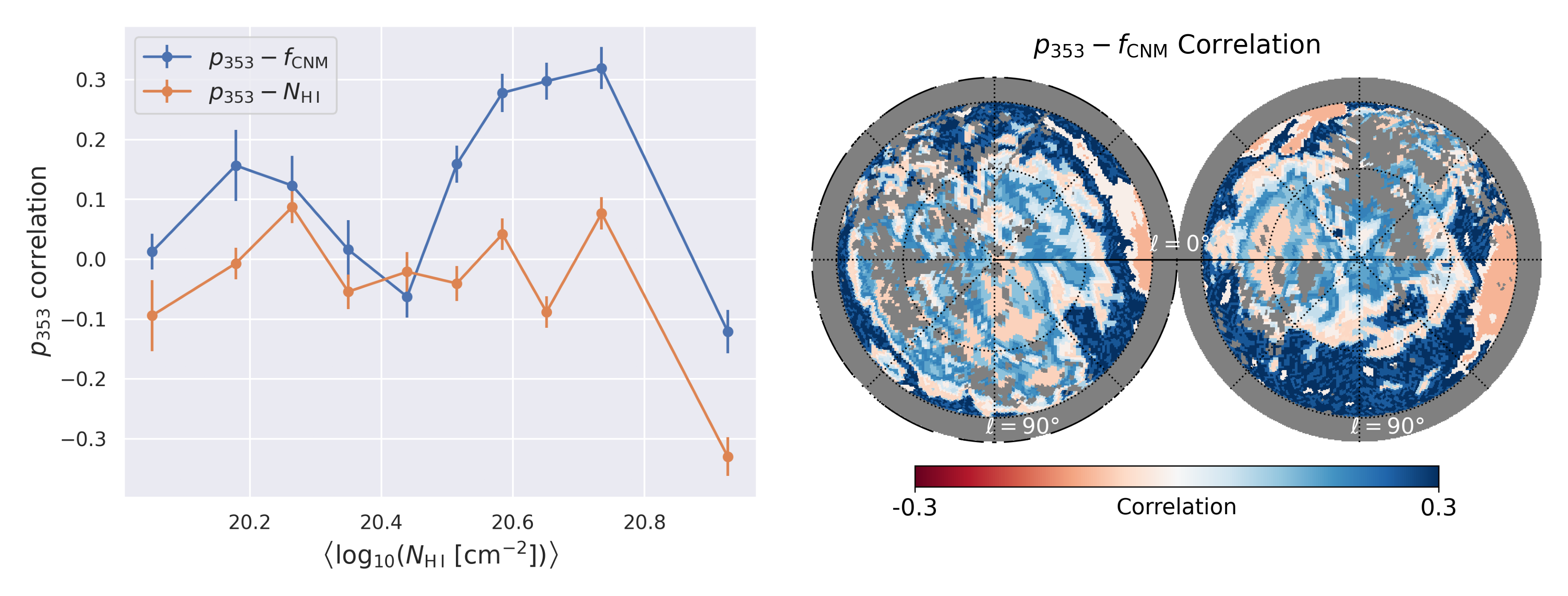
Figure 14: Column-density-binned $p_{353}$-$f_{\mathrm{CNM}}$ vs. $p_{353}$-$N_{\mathrm{H\,I}}$ correlation in the full high latitude ($|b|>30\degree$) sky using H I4PI data. Left: Spearman correlation coefficients computed in equal sightline bins of $N_{\mathrm{H\,I}}$. Right: Map of correlation between $p_{353}$ and $f_{\mathrm{CNM}}$, created by dividing the H I4PI sky into 20 equal sightline $N_{\mathrm{H\,I}}$ bins, colored by the $p_{353}$-$f_{\mathrm{CNM}}$ correlation coefficient value in each bin. The weaker positive $p_{353}$-$f_{\mathrm{CNM}}$ correlation compared to the GALFA-H I version in Figure 1 is likely attributable to the difference in $f_{\mathrm{CNM}}$ dynamic range between these two footprints as discussed in Appendix A.

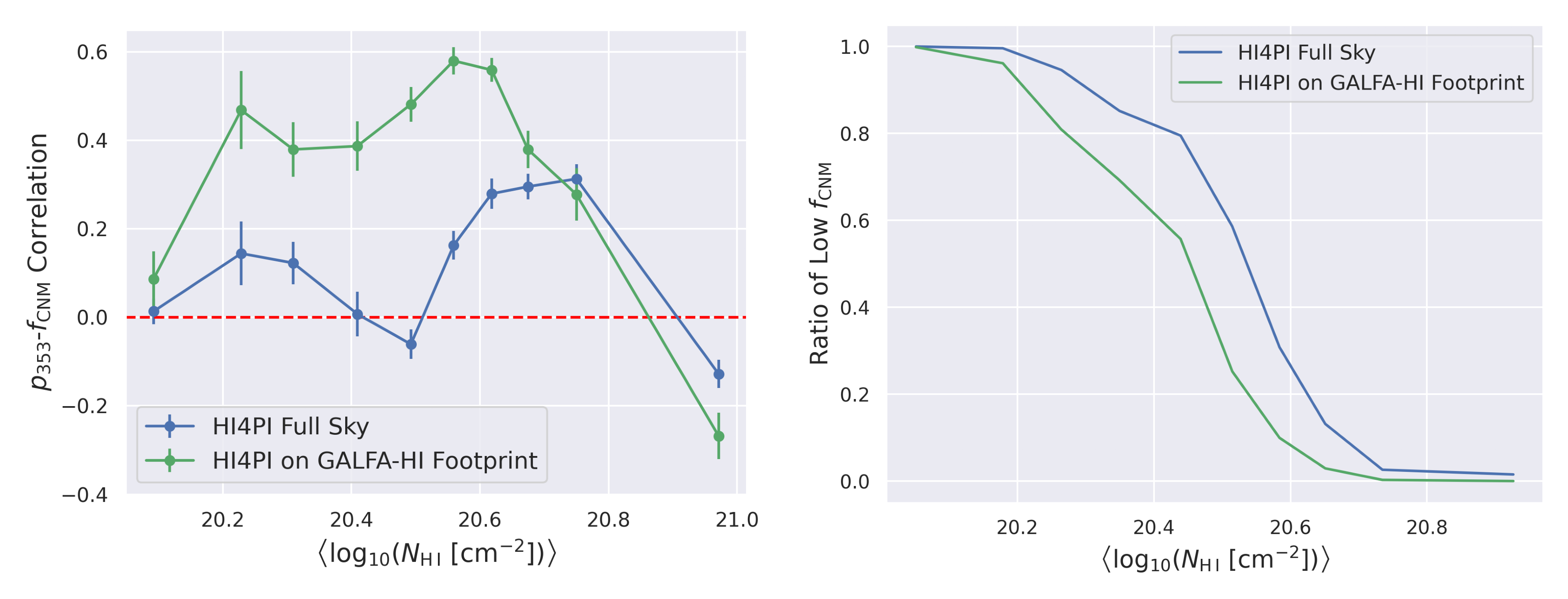
Figure 15: Left: Column-density-binned $p_{353}$-$f_{\mathrm{CNM}}$ vs. $p_{353}$-$N_{\mathrm{H\,I}}$ correlation in the high latitude ($|b|>30\degree$) sky using H I4PI data within the GALFA-H I footprint. The degree of correlation is comparable to the GALFA-H I data version in Figure 1. Right: Ratio of sightlines with $f_{\mathrm{CNM}}<\sigma_{f_{\mathrm{CNM}}}$ across the same column density bins in the H I4PI vs GALFA-H I footprints. The GALFA-H I footprint contains a significantly lower proportion of $f_{\mathrm{CNM}}\sim 0$ sightlines except in the lowest and highest $N_{\mathrm{H\,I}}$ bins.

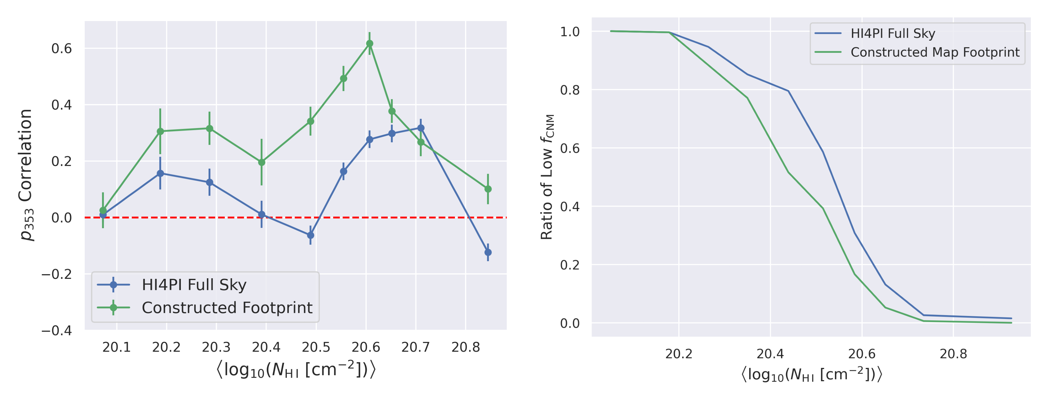
Figure 16: Left: Column-density-binned $p_{353}$-$f_{\mathrm{CNM}}$ vs. $p_{353}$-$N_{\mathrm{H\,I}}$ correlation in the test footprint discussed in Appendix A. Right: Ratio of sightlines with $f_{\mathrm{CNM}}<\sigma_{f_{\mathrm{CNM}}}$ across the same column density bins in the H I4PI vs constructed footprint. Similar to the GALFA-H I vs H I4PI comparison in Figure 15, the constructed footprint contains significantly lower proportion of $f_{\mathrm{CNM}}\sim 0$ sightlines except in the lowest and highest $N_{\mathrm{H\,I}}$ bins, and its $p_{353}$-$N_{\mathrm{H\,I}}$ correlation in these bins are correspondingly higher than the H I4PI version in Figure 15.

8 Acknowledgments

We thank Marc-Antoine Miville-Deschênes, Antoine Marchal, Peter Martin, Norm Murray, and Brandon Hensley for helpful discussions. This work was supported by the National Science Foundation under grant No. AST-2106607. This publication utilizes the Galactic ALFA HI (GALFA-H I) survey data set obtained with the Arecibo $L$-band Feed Array (ALFA) on the Arecibo 305 m telescope. The Arecibo Observatory is operated by SRI International under a cooperative agreement with the National Science Foundation (AST-1100968), and in alliance with Ana G. Méndez-Universidad Metropolitana and the Universities Space Research Association. The GALFA-H I surveys have been funded by the NSF through grants to Columbia University, the University of Wisconsin, and the University of California. This paper also makes use of observations obtained with Planck, an ESA science mission, with instruments and contributions directly funded by ESA Member States, NASA, and Canada.

Appendix A GALFA-HI and HI4PI Comparisons

Here we extend the comparison of $p_{353}$-$N_{\mathrm{H\,I}}$ vs. $p_{353}$-$f_{\mathrm{CNM}}$ correlations in different column density regimes to the full high Galactic latitude ($|b|>30\degree$) sky using H I4PI data. As described in Section 2.2, H I4PI covers the full sky at 16.2′ angular resolution. We utilize H I4PI column density and $f_{\mathrm{CNM}}$ maps smoothed to 80′ to match the $p_{353}$ resolution (HI4PI Collaboration et al., 2016; Hensley et al., 2022). Figure 15 shows the $p_{353}$-$N_{\mathrm{H\,I}}$ correlation coefficients in different column density regimes on the left, and the H I4PI version of the correlation map produced by dividing the sky into 20 equal-number-of sightline regions on the right. The $p_{353}$-$N_{\mathrm{H\,I}}$ results in the $|b|>30\degree$ H I4PI sky are consistent with our GALFA-H I results and Planck Collaboration et al. (2020), showing little correlation at lower column density, and an anticorrelation at high column densities. The correlation with $f_{\mathrm{CNM}}$ is also consistent with the GALFA-H I trends, showing a positive correlation in column density regimes where there is no $p_{353}$-$N_{\mathrm{H\,I}}$ relation, and a transition to anticorrelation at higher column densities. However, compared to the GALFA-H I result, the H I4PI $p_{353}$-$N_{\mathrm{H\,I}}$ correlation is weaker and does not extend to lower column density bins $\log_{10}(N_{\mathrm{H\,I}}\ [\mathrm{cm}^{-2}])<20.4$. While the qualitative behavior of the $p_{353}$-$f_{\rm CNM}$ relation between datasets is consistent, we explore the possible explanations for the difference in the degree of correlation.

First, since both GALFA-H I and H I4PI are smoothed to 80′ to match the $p_{353}$ resolution, the difference in their native angular resolution should not affect the $p_{353}$-$f_{\rm CNM}$ correlation results. Furthermore, when comparing the H I4PI and GALFA-H I versions of $f_{\mathrm{CNM}}$ maps, Hensley et al. (2022) found excellent agreement in overlapping regions, with a Spearman correlation coefficient of 0.97 when both maps are smoothed to the same resolution. To determine whether the differences are attributable to the data sets or to the sky areas considered, we analyze HI4PI data on the GALFA-HI footprint. Figure 15 shows the comparison between the correlation using the full H I4PI data vs. the region that overlaps GALFA-H I. The $p_{353}$-$f_{\mathrm{CNM}}$ correlation at lower column density regimes $\log_{10}(N_{\mathrm{H\,I}}\ [\mathrm{cm}^{-2}])<20.6$ is stronger for the GALFA-H I-overlapped region than the full H I4PI data sky, and is consistent with the GALFA-H I results in Figure 1. This implies that a variation in the $f_{\mathrm{CNM}}$ distribution between GALFA-H I and H I4PI footprints might play a larger role than any differences between these two datasets.

We already considered the effect of $f_{\mathrm{CNM}}$ distribution when comparing $p_{353}$-$f_{\mathrm{CNM}}$ distribution in different column density bins in Figure 2. In particular, 80% of low column density regions with $\log_{10}(N_{\mathrm{H\,I}}\ [\mathrm{cm}^{-2}])<20.40$ has $f_{\mathrm{CNM}}<0.03$. From the H I4PI version of the $f_{\mathrm{CNM}}$ map, $\sim 57\%$ of the sightlines at high latitude have $f_{\mathrm{CNM}}<0.03$, while only $\sim 44\%$ of the sightlines in the GALFA-H I footprint satisfy this condition. To further explore the effect of low CNM content, we compute the proportion of sightlines satisfying $f_{\mathrm{CNM}}<0.03$ in each column density bin examined for the $p_{353}$-$f_{\mathrm{CNM}}$ correlation and show the result in the right panel of Figure 15. In each column density bin where there is a major difference in the degree of correlation, the GALFA-H I footprint contains significantly fewer low CNM sightlines. Thus we suggest that the $p_{353}$-$f_{\mathrm{CNM}}$ correlation difference between the GALFA-H I and full H I4PI footprint is the result of differing $f_{\mathrm{CNM}}$ distribution, and specifically the proportion of low $f_{\mathrm{CNM}}$ regions where the measurement of $f_{\rm CNM}$ typically has low SNR. We examine this further by constructing a test region covering longitudes $20\degree$–$60\degree$ and $120\degree$–$160\degree$ for all latitudes. Computing $p_{353}$-$f_{\mathrm{CNM}}$ vs. $p_{353}$-$N_{\mathrm{H\,I}}$ in different column density bins, we show in Figure 16 that the test region similarly has a lower ratio of low CNM sightlines and correspondingly stronger $p_{353}$-$f_{\mathrm{CNM}}$ correlation in the same column density bins. Thus, the difference in the degree of correlation between the GALFA-H I and H I4PI datasets is likely the result of the $f_{\mathrm{CNM}}$ SNR in the sampled region, and not physical properties specific to the GALFA-H I footprint.

References

- Adak et al. (2020) Adak, D., Ghosh, T., Boulanger, F., et al. 2020, A&A, 640, A100, doi: 10.1051/0004-6361/201936124
- Andersson et al. (2015) Andersson, B. G., Lazarian, A., & Vaillancourt, J. E. 2015, ARA&A, 53, 501, doi: 10.1146/annurev-astro-082214-122414
- Astropy Collaboration et al. (2013) Astropy Collaboration, Robitaille, T. P., Tollerud, E. J., et al. 2013, A&A, 558, A33, doi: 10.1051/0004-6361/201322068
- BICEP/Keck Collaboration et al. (2022) BICEP/Keck Collaboration, :, Ade, P. A. R., et al. 2022, arXiv e-prints, arXiv:2210.05684, doi: 10.48550/arXiv.2210.05684
- Bracco et al. (2020) Bracco, A., Jelić, V., Marchal, A., et al. 2020, A&A, 644, L3, doi: 10.1051/0004-6361/202039283
- Burstein & Heiles (1978) Burstein, D., & Heiles, C. 1978, ApJ, 225, 40, doi: 10.1086/156466
- Campbell et al. (2022) Campbell, J. L., Clark, S. E., Gaensler, B. M., et al. 2022, ApJ, 927, 49, doi: 10.3847/1538-4357/ac400d
- Chen et al. (2019) Chen, C.-Y., King, P. K., Li, Z.-Y., Fissel, L. M., & Mazzei, R. R. 2019, MNRAS, 485, 3499, doi: 10.1093/mnras/stz618
- Clark (2018) Clark, S. E. 2018, ApJ, 857, L10, doi: 10.3847/2041-8213/aabb54
- Clark & Hensley (2019) Clark, S. E., & Hensley, B. S. 2019, ApJ, 887, 136, doi: 10.3847/1538-4357/ab5803
- Clark et al. (2015) Clark, S. E., Hill, J. C., Peek, J. E. G., Putman, M. E., & Babler, B. L. 2015, Phys. Rev. Lett., 115, 241302, doi: 10.1103/PhysRevLett.115.241302
- Clark et al. (2019) Clark, S. E., Peek, J. E. G., & Miville-Deschênes, M. A. 2019, ApJ, 874, 171, doi: 10.3847/1538-4357/ab0b3b
- Clark et al. (2014) Clark, S. E., Peek, J. E. G., & Putman, M. E. 2014, ApJ, 789, 82, doi: 10.1088/0004-637X/789/1/82
- Crutcher (2012) Crutcher, R. M. 2012, ARA&A, 50, 29, doi: 10.1146/annurev-astro-081811-125514
- Dickey et al. (2013) Dickey, J. M., McClure-Griffiths, N., Gibson, S. J., et al. 2013, PASA, 30, e003, doi: 10.1017/pasa.2012.003
- Dickey et al. (2022) Dickey, J. M., Dempsey, J. M., Pingel, N. M., et al. 2022, ApJ, 926, 186, doi: 10.3847/1538-4357/ac3a89
- Draine (2011) Draine, B. T. 2011, Physics of the Interstellar and Intergalactic Medium (Princeton University Press)
- Draine & Fraisse (2009) Draine, B. T., & Fraisse, A. A. 2009, ApJ, 696, 1, doi: 10.1088/0004-637X/696/1/1
- Draine & Hensley (2021) Draine, B. T., & Hensley, B. S. 2021, ApJ, 919, 65, doi: 10.3847/1538-4357/ac0050
- Draine & Weingartner (1996) Draine, B. T., & Weingartner, J. C. 1996, ApJ, 470, 551, doi: 10.1086/177887
- Ferrière (2001) Ferrière, K. M. 2001, Reviews of Modern Physics, 73, 1031, doi: 10.1103/RevModPhys.73.1031
- Fiege & Pudritz (2000) Fiege, J. D., & Pudritz, R. E. 2000, ApJ, 544, 830, doi: 10.1086/317228
- Field et al. (1969) Field, G. B., Goldsmith, D. W., & Habing, H. J. 1969, ApJ, 155, L149, doi: 10.1086/180324
- Fielding et al. (2023) Fielding, D. B., Ripperda, B., & Philippov, A. A. 2023, ApJ, 949, L5, doi: 10.3847/2041-8213/accf1f
- Fissel et al. (2016) Fissel, L. M., Ade, P. A. R., Angilè, F. E., et al. 2016, ApJ, 824, 134, doi: 10.3847/0004-637X/824/2/134
- Gazol & Villagran (2021) Gazol, A., & Villagran, M. A. 2021, MNRAS, 501, 3099, doi: 10.1093/mnras/staa3852
- Ghosh et al. (2017) Ghosh, T., Boulanger, F., Martin, P. G., et al. 2017, A&A, 601, A71, doi: 10.1051/0004-6361/201629829
- Górski et al. (2005) Górski, K. M., Hivon, E., Banday, A. J., et al. 2005, ApJ, 622, 759, doi: 10.1086/427976
- Guillet et al. (2018) Guillet, V., Fanciullo, L., Verstraete, L., et al. 2018, A&A, 610, A16, doi: 10.1051/0004-6361/201630271
- Halal et al. (2023) Halal, G., Clark, S. E., Cukierman, A., Beck, D., & Kuo, C.-L. 2023, arXiv e-prints, arXiv:2306.10107, doi: 10.48550/arXiv.2306.10107
- Han (2017) Han, J. L. 2017, ARA&A, 55, 111, doi: 10.1146/annurev-astro-091916-055221
- Haud & Kalberla (2007) Haud, U., & Kalberla, P. M. W. 2007, A&A, 466, 555, doi: 10.1051/0004-6361:20065796
- Heiles & Troland (2003) Heiles, C., & Troland, T. H. 2003, ApJ, 586, 1067, doi: 10.1086/367828
- Hensley & Draine (2021) Hensley, B. S., & Draine, B. T. 2021, ApJ, 906, 73, doi: 10.3847/1538-4357/abc8f1
- Hensley & Draine (2022) —. 2022, arXiv e-prints, arXiv:2208.12365, doi: 10.48550/arXiv.2208.12365
- Hensley et al. (2022) Hensley, B. S., Murray, C. E., & Dodici, M. 2022, ApJ, 929, 23, doi: 10.3847/1538-4357/ac5cbd
- HI4PI Collaboration et al. (2016) HI4PI Collaboration, Ben Bekhti, N., Flöer, L., et al. 2016, A&A, 594, A116, doi: 10.1051/0004-6361/201629178
- Hoang & Lazarian (2008) Hoang, T., & Lazarian, A. 2008, MNRAS, 388, 117, doi: 10.1111/j.1365-2966.2008.13249.x
- Hoang et al. (2022) Hoang, T. D., Ngoc, N. B., Diep, P. N., et al. 2022, ApJ, 929, 27, doi: 10.3847/1538-4357/ac5abf
- Hunter (2007) Hunter, J. D. 2007, Computing in Science and Engineering, 9, 90, doi: 10.1109/MCSE.2007.55
- Inoue & Inutsuka (2016) Inoue, T., & Inutsuka, S.-i. 2016, ApJ, 833, 10, doi: 10.3847/0004-637X/833/1/10
- Jelić et al. (2018) Jelić, V., Prelogović, D., Haverkorn, M., Remeijn, J., & Klindžić, D. 2018, A&A, 615, L3, doi: 10.1051/0004-6361/201833291
- Kalberla & Haud (2018) Kalberla, P. M. W., & Haud, U. 2018, A&A, 619, A58, doi: 10.1051/0004-6361/201833146
- Kalberla & Kerp (2009) Kalberla, P. M. W., & Kerp, J. 2009, ARA&A, 47, 27, doi: 10.1146/annurev-astro-082708-101823
- Kalberla & Kerp (2016) Kalberla, P. M. W., & Kerp, J. 2016, A&A, 595, A37, doi: 10.1051/0004-6361/201629113
- Kim & Ostriker (2017) Kim, C.-G., & Ostriker, E. C. 2017, ApJ, 846, 133, doi: 10.3847/1538-4357/aa8599
- Kim et al. (2013) Kim, C.-G., Ostriker, E. C., & Kim, W.-T. 2013, ApJ, 776, 1, doi: 10.1088/0004-637X/776/1/1
- Kim et al. (2014) —. 2014, ApJ, 786, 64, doi: 10.1088/0004-637X/786/1/64
- Kirchschlager et al. (2019) Kirchschlager, F., Bertrang, G. H. M., & Flock, M. 2019, MNRAS, 488, 1211, doi: 10.1093/mnras/stz1763
- Lei & Clark (2023) Lei, M., & Clark, S. E. 2023, ApJ, 947, 74, doi: 10.3847/1538-4357/acc02a
- Lenz et al. (2017) Lenz, D., Hensley, B. S., & Doré, O. 2017, ApJ, 846, 38, doi: 10.3847/1538-4357/aa84af
- Letessier-Selvon & Stanev (2011) Letessier-Selvon, A., & Stanev, T. 2011, Reviews of Modern Physics, 83, 907, doi: 10.1103/RevModPhys.83.907
- Marchal et al. (2019) Marchal, A., Miville-Deschênes, M.-A., Orieux, F., et al. 2019, A&A, 626, A101, doi: 10.1051/0004-6361/201935335
- Martínez-Solaeche et al. (2018) Martínez-Solaeche, G., Karakci, A., & Delabrouille, J. 2018, MNRAS, 476, 1310, doi: 10.1093/mnras/sty204
- McBride et al. (2023) McBride, L., Bull, P., & Hensley, B. S. 2023, MNRAS, 519, 4370, doi: 10.1093/mnras/stac3754
- McClure-Griffiths et al. (2006) McClure-Griffiths, N. M., Dickey, J. M., Gaensler, B. M., Green, A. J., & Haverkorn, M. 2006, ApJ, 652, 1339, doi: 10.1086/508706
- McClure-Griffiths et al. (2009) McClure-Griffiths, N. M., Pisano, D. J., Calabretta, M. R., et al. 2009, ApJS, 181, 398, doi: 10.1088/0067-0049/181/2/398
- McClure-Griffiths et al. (2015) McClure-Griffiths, N. M., Stanimirovic, S., Murray, C., et al. 2015, PoS, AASKA14, 130, doi: 10.22323/1.215.0130
- Moseley et al. (2021) Moseley, E. R., Draine, B. T., Tomida, K., & Stone, J. M. 2021, MNRAS, 500, 3290, doi: 10.1093/mnras/staa3384
- Murray et al. (2020) Murray, C. E., Peek, J. E. G., & Kim, C.-G. 2020, ApJ, 899, 15, doi: 10.3847/1538-4357/aba19b
- Murray et al. (2018) Murray, C. E., Stanimirović, S., Goss, W. M., et al. 2018, ApJS, 238, 14, doi: 10.3847/1538-4365/aad81a
- Nguyen et al. (2018) Nguyen, H., Dawson, J. R., Miville-Deschênes, M. A., et al. 2018, ApJ, 862, 49, doi: 10.3847/1538-4357/aac82b
- Panopoulou et al. (2019) Panopoulou, G. V., Hensley, B. S., Skalidis, R., Blinov, D., & Tassis, K. 2019, A&A, 624, L8, doi: 10.1051/0004-6361/201935266
- Panopoulou & Lenz (2020) Panopoulou, G. V., & Lenz, D. 2020, ApJ, 902, 120, doi: 10.3847/1538-4357/abb6f5
- Peek & Clark (2019) Peek, J. E. G., & Clark, S. E. 2019, ApJ, 886, L13, doi: 10.3847/2041-8213/ab53de
- Peek et al. (2018) Peek, J. E. G., Babler, B. L., Zheng, Y., et al. 2018, ApJS, 234, 2, doi: 10.3847/1538-4365/aa91d3
- Pelgrims et al. (2021) Pelgrims, V., Clark, S. E., Hensley, B. S., et al. 2021, A&A, 647, A16, doi: 10.1051/0004-6361/202040218
- Pelkonen et al. (2007) Pelkonen, V. M., Juvela, M., & Padoan, P. 2007, A&A, 461, 551, doi: 10.1051/0004-6361:20065838
- Planck Collaboration et al. (2015a) Planck Collaboration, Ade, P. A. R., Aghanim, N., et al. 2015a, A&A, 576, A104, doi: 10.1051/0004-6361/201424082
- Planck Collaboration et al. (2015b) —. 2015b, A&A, 576, A105, doi: 10.1051/0004-6361/201424086
- Planck Collaboration et al. (2016) Planck Collaboration, Aghanim, N., Alves, M. I. R., et al. 2016, A&A, 596, A105, doi: 10.1051/0004-6361/201628636
- Planck Collaboration et al. (2020) Planck Collaboration, Aghanim, N., Akrami, Y., et al. 2020, A&A, 641, A12, doi: 10.1051/0004-6361/201833885
- Plaszczynski et al. (2014) Plaszczynski, S., Montier, L., Levrier, F., & Tristram, M. 2014, MNRAS, 439, 4048, doi: 10.1093/mnras/stu270
- Polson & Scott (2011) Polson, N. G., & Scott, J. G. 2011, arXiv e-prints, arXiv:1104.4937, doi: 10.48550/arXiv.1104.4937
- Remazeilles et al. (2011) Remazeilles, M., Delabrouille, J., & Cardoso, J.-F. 2011, MNRAS, 418, 467, doi: 10.1111/j.1365-2966.2011.19497.x
- Riener et al. (2020) Riener, M., Kainulainen, J., Beuther, H., et al. 2020, A&A, 633, A14, doi: 10.1051/0004-6361/201936814
- Salvatier et al. (2016) Salvatier, J., Wiecki, T. V., & Fonnesbeck, C. 2016, PeerJ Computer Science, 2, e55, doi: 10.7717/peerj-cs.55
- Saury et al. (2014) Saury, E., Miville-Deschênes, M. A., Hennebelle, P., Audit, E., & Schmidt, W. 2014, A&A, 567, A16, doi: 10.1051/0004-6361/201321113
- Sullivan et al. (2021) Sullivan, C. H., Fissel, L. M., King, P. K., et al. 2021, MNRAS, 503, 5006, doi: 10.1093/mnras/stab596
- Tassis & Pavlidou (2015) Tassis, K., & Pavlidou, V. 2015, MNRAS, 451, L90, doi: 10.1093/mnrasl/slv077
- Vacher et al. (2023) Vacher, L., Aumont, J., Boulanger, F., et al. 2023, A&A, 672, A146, doi: 10.1051/0004-6361/202245292
- van der Walt et al. (2011) van der Walt, S., Colbert, S. C., & Varoquaux, G. 2011, Computing in Science and Engineering, 13, 22, doi: 10.1109/MCSE.2011.37
- Virtanen et al. (2020) Virtanen, P., Gommers, R., Oliphant, T. E., et al. 2020, Nature Methods, 17, 261, doi: 10.1038/s41592-019-0686-2
- Winkel et al. (2016) Winkel, B., Kerp, J., Flöer, L., et al. 2016, A&A, 585, A41, doi: 10.1051/0004-6361/201527007
- Wolfire et al. (2003) Wolfire, M. G., McKee, C. F., Hollenbach, D., & Tielens, A. G. G. M. 2003, ApJ, 587, 278, doi: 10.1086/368016
- Zaroubi et al. (2015) Zaroubi, S., Jelic, V., de Bruyn, A. G., et al. 2015, MNRAS, 454, L46, doi: 10.1093/mnrasl/slv123