QSlack: A slack-variable approach for variational quantum semi-definite programming

Abstract

Solving optimization problems is a key task for which quantum computers could possibly provide a speedup over the best known classical algorithms. Particular classes of optimization problems including semi-definite programming (SDP) and linear programming (LP) have wide applicability in many domains of computer science, engineering, mathematics, and physics. Here we focus on semi-definite and linear programs for which the dimensions of the variables involved are exponentially large, so that standard classical SDP and LP solvers are not helpful for such large-scale problems. We propose the QSlack and CSlack methods for estimating their optimal values, respectively, which work by 1) introducing slack variables to transform inequality constraints to equality constraints, 2) transforming a constrained optimization to an unconstrained one via the penalty method, and 3) replacing the optimizations over all possible non-negative variables by optimizations over parameterized quantum states and parameterized probability distributions. Under the assumption that the SDP and LP inputs are efficiently measurable observables, it follows that all terms in the resulting objective functions are efficiently estimable by either a quantum computer in the SDP case or a quantum or probabilistic computer in the LP case. Furthermore, by making use of SDP and LP duality theory, we prove that these methods provide a theoretical guarantee that, if one could find global optima of the objective functions, then the resulting values sandwich the true optimal values from both above and below. Finally, we showcase the QSlack and CSlack methods on a variety of example optimization problems and discuss details of our implementation, as well as the resulting performance. We find that our implementations of both the primal and dual for these problems approach the ground truth, typically achieving errors of the order $10^{-2}$.

LABEL:FirstPage1 LABEL:LastPage#1102

I Introduction

Quantum computation has arisen in the past few decades as a viable model of computing, understood quite well by now from a theoretical perspective [41] and undergoing rapid development from the experimental viewpoint [17, 108, 114, 34, 99]. It has garnered so much interest from a wide variety of scientists, engineers, and mathematicians due to the promise of speedups over the best known classical algorithms, for tasks such as factoring products of prime integers [115, 116], unstructured search [53, 54], simulation of physics [78, 11, 75] and chemistry [33, 88], learning features of solutions to linear systems of equations [62, 40], and machine learning [73, 47].

Another target application of quantum computing is in solving optimization problems [86, 10], again with the hope of achieving a speedup over the best known classical algorithms. There have long been various investigations of applying quantum simulated annealing to quadratic unconstrained binary optimization problems [144]; here instead, we focus on different subclasses of optimization problems, known as semi-definite and linear programming.

Semi-definite programming refers to a class of optimization problems involving a linear objective function optimized over the cone of positive semi-definite operators intersected with an affine space [27, 142]. Solving semi-definite programs (SDPs) has wide applications across many different fields, including combinatorial optimization [51, 106, 126], finance [49], job scheduling in operations research [120], machine learning [39, 56, 89], physics [83, 19, 113, 20, 44], and quantum information science [135, 123, 112]. Furthermore, many algorithms for solving SDPs efficiently on classical computers are now known and in extensive use [102, 4, 5, 80] (by “efficiently,” here we mean that the algorithms have runtime polynomial in the dimension of the matrices involved).

The wide applications of SDPs and the tantalizing possibility of achieving quantum speedup for them have motivated a number of researchers to investigate quantum algorithms for solving SDPs [25, 129, 22, 130, 71, 98, 9, 21, 141, 100]. Researchers have previously considered several approaches for this problem. A number of proposals have guaranteed runtimes and are intended to be executed on fault-tolerant quantum computers [25, 129, 22, 130, 71, 9, 141]; as such, it is not expected that the promised speedups of these algorithms will be realized in the near term. Another approach consists of hybrid quantum-classical computations [21], in which a given SDP involves terms expressed as expectations of observables, so that these terms can be efficiently estimated on a quantum computer and fed into a classical SDP solver that produces an approximate solution to the SDP. The main regime of interest for all of these algorithms is when the matrices involved in the optimization are large (i.e., of dimension $2^{n}\times 2^{n}$, where $n$ is a parameter) and such that expressions like $\operatorname{Tr}[AX]$ for Hermitian $A$ and positive semi-definite $X$ can be efficiently estimated on quantum computers but not so using the best known classical algorithms.

In this paper, we focus on the variational approach to solving SDPs on quantum computers, which we call variational quantum semi-definite programming. While this approach has been explored in some recent papers [98, 100], our main theoretical contribution here is a method that theoretically guarantees lower and upper bounds on the optimal value of a given SDP. We do so by introducing slack variables into both the primal and dual SDPs, which are physically realized as either parameterized states or observables. Since slack variables transform inequality constraints to equality constraints, we can then move all of the resulting equality constraints into penalty terms in the objective function of the SDP, leaving an unconstrained optimization problem. We express the aforementioned penalty terms in terms of the Hilbert–Schmidt distance, and as such, each of the penalty terms can be evaluated on a quantum computer as expectations of observables, by means of the destructive swap test [48], which is also known more recently as Bell sampling [92, 60], or by means of a mixed-state Loschmidt echo test that we introduce here (see Appendix D.2.2).

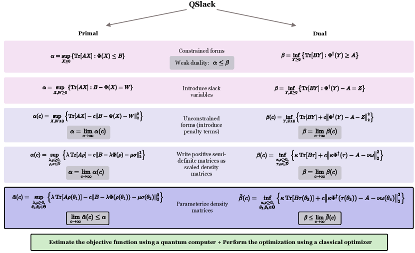
Figure 1: Overview of the QSlack method introduced in our paper. From top to bottom, we modify the expressions of the primal and dual semi-definite programs to a form that can be evaluated on a quantum computer. Section II.1 provides details for the first three rows, and Section II.2 provides details for the last two rows. The same ideas lead to the CSlack method for solving linear programs, as discussed in Sections III.1 and III.2.

Our approach is thus a hybrid quantum–classical optimization, only using a quantum computer to evaluate expectations of observables or to perform the destructive swap test, and leaving all other computations to a classical computer. As such, our algorithm falls within the large and increasingly studied class of variational quantum algorithms [28, 12]. Using this approach for both the primal and dual SDPs, we can guarantee lower and upper bounds on the optimal value of the optimization problem, thus solving a key question left open in [98]. We describe our method in far more detail in Section II.2, after recalling some background on semi-definite programming in Section II.1. Since a key feature of our algorithm is the introduction of slack variables physically realized as parameterized states or observables (i.e., “quantum slack variables”), we call it the QSlack method. Figure 1 summarizes the main ideas behind QSlack.

We also delineate a classical variant of our method for approximately solving linear programs. Indeed, a linear program (LP) involves the optimization of a linear objective function over the positive orthant intersected with an affine space. As such, our approach here again involves introducing slack variables into both the primal and dual LPs, which are realized as either parameterized probability distributions or parameterized observable vectors (these are the classical reductions of parameterized states and observables, respectively). Our approach can thus be called a variational linear programming algorithm, and we refer to it as the CSlack method.

Similar to QSlack, the CSlack method transforms inequality constraints to equality constraints by means of parameterized slack variables, and all equality constraints are then moved into the objective function as penalty terms, so that the resulting problem is an unconstrained optimization. This method guarantees lower and upper bounds on the optimal value of the LP. Let us note that a similar method for solving linear programs on quantum computers was recently introduced [76], with a key difference between our approach and theirs being that they do not make use of slack variables.

Another key contribution of our paper is to show how the QSlack method can be applied to a wide variety of examples, focusing on problems of interest in physics and quantum information science. In particular, we apply the QSlack method to estimating the trace distance, fidelity, entanglement negativity, and constrained minimum energy of Hamiltonians. We have conducted extensive numerical simulations of the QSlack method in order to understand how it would perform in practice on quantum computers. For the examples considered, we find that the QSlack method works well, leading to lower and upper bounds on the optimal value of a given optimization problem. Although we made use of parameterized quantum circuits in our simulations (via the purification ansatz and the convex-combination ansatz), let us stress here that the general QSlack method is compatible with other parameterizations of quantum states, such as quantum Boltzmann machines [1, 133], which can be explored in future work. We also apply the CSlack method to example LPs of interest and showcase its performance.

Our numerical simulations provide practical evidence of the QSlack and CSlack methods’ ability to bound optimal values from above and below. Due to the number of parameters and terms in the modified objective functions, training CSlack and QSlack objectives is observed to be relatively slow and noisy, as compared to a standard variational quantum eigensolver. However, with our choices of hyperparameters, we observe consistent convergence to the true value, typically achieving an error on the order of $10^{-2}$, giving preliminary evidence of the potential versatility and practicality of our method.

The remainder of our paper proceeds as follows. We first provide details of the QSlack method in Section II, beginning by recalling basic aspects of semi-definite programming (Section II.1) and following with an overview of the QSlack algorithm (Section II.2). Then we formulate several example problems of interest in quantum information and physics in the QSlack framework (Section II.3), after which we provide details of how we simulated the QSlack algorithms and then we discuss the results of our numerical experiments (Section II.4). We then mirror this structure for CSlack, giving background on linear programming (Section III.1), the CSlack algorithm (Section III.2), examples (Section III.3), and details of simulations (Section III.4). Finally, we conclude in Section IV with a summary and directions for future research. All of the appendices provide even greater details of the methods underlying our approach.

II QSlack background, algorithm, examples, and simulations

II.1 Background on semi-definite programming

Let us begin by recalling the basics of semi-definite programming, following the formulation of [138, page 223] (see also [72, Section 2.4]). Fix $d_{1},d_{2}\in\mathbb{N}$. Let $A$ be a $d_{1}\times d_{1}$ Hermitian matrix, $B$ a $d_{2}\times d_{2}$ Hermitian matrix, and $\Phi$ a Hermiticity-preserving superoperator that takes $d_{1}\times d_{1}$ Hermitian matrices to $d_{2}\times d_{2}$ Hermitian matrices. A semi-definite program is specified by the triple $(A,B,\Phi)$ and is defined as the following optimization problem:

$$\alpha\coloneqq\sup_{X\geq 0}\left\{\operatorname{Tr}[AX]:\Phi(X)\leq B\right\},$$ (1)

where the supremum optimization is over every $d_{1}\times d_{1}$ positive semi-definite matrix $X$ (i.e., $X\geq 0$ is a shorthand notation for $X$ being positive semi-definite) and the inequality constraint $\Phi(X)\leq B$ is equivalent to $B-\Phi(X)$ being a positive semi-definite matrix. We call the optimization in (1) the primal SDP. A matrix $X$ is feasible for the optimization in (1) if both constraints $X\geq 0$ and $\Phi(X)\leq B$ are satisfied; such an $X$ is also said to be primal feasible.

The dual optimization problem is as follows:

$$\beta\coloneqq\inf_{Y\geq 0}\left\{\operatorname{Tr}[BY]:\Phi^{{\dagger}}(Y)\geq A\right\},$$ (2)

where the infimum optimization is over every $d_{2}\times d_{2}$ positive semi-definite matrix $Y$ and again the inequality constraint $\Phi^{{\dagger}}(Y)\geq A$ is equivalent to $\Phi^{{\dagger}}(Y)-A$ being a positive semi-definite matrix. Additionally, $\Phi^{{\dagger}}$ is a Hermiticity preserving superoperator that is the adjoint of $\Phi$; i.e., it satisfies

$$\left\langle Y,\Phi(X)\right\rangle=\left\langle\Phi^{{\dagger}}(Y),X\right\rangle$$ (3)

for every $d_{1}\times d_{1}$ matrix $X$ and every $d_{2}\times d_{2}$ matrix $Y$, where the Hilbert–Schmidt inner product is defined for square matrices $C$ and $D$ as

$$\left\langle C,D\right\rangle\coloneqq\operatorname{Tr}[C^{{\dagger}}D].$$ (4)

A matrix $Y$ is dual feasible if both constraints $Y\geq 0$ and $\Phi^{{\dagger}}(Y)\geq A$ are satisfied.

Semi-definite programming is equipped with a duality theory, which is helpful for both numerical and analytical purposes. Weak duality corresponds to the inequality

$$\alpha\leq\beta.$$ (5)

As a consequence of weak duality, an arbitrary primal feasible $X$ leads to a lower bound on the optimal value because $\operatorname{Tr}[AX]\leq\alpha$ for all such $X$, and an arbitrary dual feasible $Y$ leads to an upper bound on the optimal value because $\beta\leq\operatorname{Tr}[BY]$ for such a $Y$. By producing a primal feasible $X$ and a dual feasible $Y$, we can thus sandwich the optimal values of the primal and dual SDPs with guaranteed lower and upper bounds. Strong duality corresponds to the equality

$$\alpha=\beta,$$ (6)

and it holds whenever Slater’s condition is satisfied. Slater’s condition often holds in practice and corresponds to there existing a primal feasible $X$ and a strictly dual feasible $Y$ (i.e., the strict inequalities $Y>0$ and $\Phi^{{\dagger}}(Y)>A$ hold). Alternatively, Slater’s condition holds if there exists a strictly primal feasible $X$ and a dual feasible $Y$.

One can introduce slack variables that transform the inequality constraints in (1) and (2) to equality constraints. To see how this works, recall that the inequality $\Phi(X)\leq B$ is a shorthand for $B-\Phi(X)$ being a positive semi-definite matrix. As such, this latter condition is equivalent to the existence of a $d_{2}\times d_{2}$ positive semi-definite matrix $W$ such that $B-\Phi(X)=W$. We can then rewrite the optimization in (1) as follows:

$$\alpha=\sup_{X,W\geq 0}\left\{\operatorname{Tr}[AX]:B-\Phi(X)=W\right\}.$$ (7)

By similar reasoning, we can rewrite the dual SDP in (2) as follows:

$$\beta=\inf_{Y,Z\geq 0}\left\{\operatorname{Tr}[BY]:\Phi^{{\dagger}}(Y)-A=Z\right\},$$ (8)

where $Z$ is a $d_{1}\times d_{1}$ matrix.

The final observation that we recall in this review is that it is possible to transform the constrained optimizations in (7) and (8) to unconstrained optimizations by introducing penalty terms in the objective functions. Let us define the Hilbert–Schmidt norm of an operator $C$ as

$$\left\|C\right\|_{2}\coloneqq\sqrt{\left\langle C,C\right\rangle},$$ (9)

which has the key property of being faithful: $C=0$ if and only if $\left\|C\right\|_{2}=0$. As such, we can modify the optimizations as follows:

$$\alpha(c) \coloneqq\sup_{X,W\geq 0}\left\{\operatorname{Tr}[AX]-c\left\|B-\Phi(X)-W\right\|_{2}^{2}\right\},$$ (10)

$$\beta(c) \coloneqq\inf_{Y,Z\geq 0}\left\{\operatorname{Tr}[BY]+c\left\|\Phi^{{\dagger}}(Y)-A-Z\right\|_{2}^{2}\right\},$$ (11)

where $c>0$ is a penalty constant. The following equalities hold from standard reasoning regarding the penalty method (specifically, see [15, Proposition 5.2.1] with $\lambda_{k}=0$ for all $k$):

$$\alpha=\lim_{c\rightarrow\infty}\alpha(c),\qquad\beta=\lim_{c\rightarrow\infty}\beta(c),$$ (12)

and they give us a way to approximate the optimal values $\alpha$ and $\beta$, respectively, by means of a sequence of unconstrained optimizations. The reductions from (1) to (10) and from (2) to (11) are well known, but they constitute some of the core preliminary observations behind our QSlack method. See the first three rows of Figure 1 for a summary of these steps.

In Appendix A, we discuss some variants of $\alpha(c)$ and $\beta(c)$ that have the additional feature of weak duality holding for every $c>0$. It is also of interest to consider SDPs and LPs with both equality and inequality constraints. We discuss these cases in Appendix B, along with the QSlack and CSlack methods for them.

II.2 QSlack algorithm for variational quantum semi-definite programming

As indicated previously, one of the basic ideas of the QSlack algorithm is to solve the primal and dual SDPs in (1)–(2) by employing their reductions to (10)–(11), respectively. Additionally, some of the core assumptions are the same as those made in [98]: we assume that the Hermitian matrices $A$ and $B$ are observables that can be efficiently measured on a quantum computer, and we assume that the Hermiticity-preserving superoperator$~{}\Phi$ corresponds to one also. Particular examples of efficiently measurable observables and input models for $A$, $B$, and $\Phi$ are detailed in Appendix C. As such, now we assume that $d_{1}=2^{n}$ and $d_{2}=2^{m}$ for $n,m\in\mathbb{N}$, so that $A$ is an $n$-qubit observable and $B$ is an $m$-qubit observable, and the superoperator $\Phi$ maps $n$-qubit observables to $m$-qubit observables. Furthermore, we expect these SDPs to be difficult to solve on classical computers, given that standard algorithms for solving SDPs have runtime polynomial in the dimensions of the inputs $A$, $B$, and $\Phi$, which are now exponential in $n$, $m$, or both.

We employ another basic observation also used in [98]: the positive semi-definite matrices $X$, $W$, $Y$, and $Z$ appearing in the optimizations in (10) and (11) can be represented as scaled density matrices. That is, whenever $X\neq 0$, it can be written as $X=\lambda\rho$, where $\lambda\coloneqq\operatorname{Tr}[X]$ and $\rho\coloneqq X/\lambda$, so that $\lambda>0$ and $\rho$ is a density matrix, satisfying $\rho\geq 0$ and $\operatorname{Tr}[\rho]=1$. This observation implies that the optimizations in (10)–(11) can be rewritten as follows, respectively:

$$\alpha(c) =\sup_{\begin{subarray}{c}\lambda,\mu\geq 0,\\ \rho,\sigma\in\mathcal{D}\end{subarray}}\left\{\lambda\operatorname{Tr}[A\rho]-c\left\|B-\lambda\Phi(\rho)-\mu\sigma\right\|_{2}^{2}\right\},$$ (13)

$$\beta(c) =\inf_{\begin{subarray}{c}\kappa,\nu\geq 0,\\ \tau,\omega\in\mathcal{D}\end{subarray}}\left\{\kappa\operatorname{Tr}[B\tau]+c\left\|\kappa\Phi^{{\dagger}}(\tau)-A-\nu\omega\right\|_{2}^{2}\right\},$$ (14)

where we have simply made the substitutions $X=\lambda\rho$, $W=\mu\sigma$, $Y=\kappa\tau$, and $Z=\nu\omega$, and $\mathcal{D}$ denotes the set of all density matrices.

One can interpret what we are doing here as taking advantage of the mathematical structure of quantum mechanics, namely, that states are constrained to be positive semi-definite matrices, in order to impose the positive semi-definite constraints on $X$, $W$, $Y$, and $Z$. Alternatively, as happens in some of the examples that we explore in Section II.3, if any of the matrices in the optimization are not constrained to be positive semi-definite and are general or Hermitian, then we can write them as a linear combination of Pauli matrices with complex or real coefficients, respectively.

Expressions like $\operatorname{Tr}[A\rho]$ and $\operatorname{Tr}[B\tau]$ in (13)–(14) are interpreted in quantum mechanics in terms of the Born rule and are understood as expectations of the observables $A$ and $B$ with respect to the states $\rho$ and $\tau$, respectively. As such, in principle, the quantities $\operatorname{Tr}[A\rho]$ and $\operatorname{Tr}[B\tau]$ can be estimated through repetition, by repeatedly preparing the states $\rho$ and $\tau$, performing the procedures to measure the observables $A$ and $B$, and finally calculating sample means as estimates of $\operatorname{Tr}[A\rho]$ and $\operatorname{Tr}[B\tau]$. In Appendix E, we discuss how the other terms $\left\|B-\lambda\Phi(\rho)-\mu\sigma\right\|_{2}^{2}$ and $\left\|\kappa\Phi^{{\dagger}}(\tau)-A-\nu\omega\right\|_{2}^{2}$ can be estimated, for which the destructive swap test [48] or the mixed-state Loschmidt echo test (Appendix D.2.2) are helpful.

While the modifications in (13)–(14) allow for rewriting the objective functions in (10)–(11) in terms of expectations of observables, evaluating the objective functions in (13)–(14) is still too difficult: the optimizations are over all possible states and not all states are efficiently preparable. That is, even if the observables are efficiently measurable, the overall procedure will not be efficient if there is not an efficient method to prepare the states $\rho$ and$~{}\tau$. Thus, our next modification is to replace the optimizations over all possible states in (13)–(14) with optimizations over parameterized states that are efficiently preparable, leading to the following:

$$\tilde{\alpha}(c) \coloneqq\sup_{\lambda,\mu\geq 0,\theta_{1},\theta_{2}\in\Theta}\Big{\{}\lambda\operatorname{Tr}[A\rho(\theta_{1})]$$

$$\qquad\qquad-c\left\|B-\lambda\Phi(\rho(\theta_{1}))-\mu\sigma(\theta_{2})\right\|_{2}^{2}\Big{\}},$$ (15)

$$\tilde{\beta}(c) \coloneqq\inf_{\kappa,\nu\geq 0,\theta_{3},\theta_{4}\in\Theta}\Big{\{}\kappa\operatorname{Tr}[B\tau(\theta_{3})]$$

$$\qquad\qquad+c\left\|\kappa\Phi^{{\dagger}}(\tau(\theta_{3}))-A-\nu\omega(\theta_{4})\right\|_{2}^{2}\Big{\}},$$ (16)

where $\Theta$ is a general set of parameter values, $\theta_{1}$, $\theta_{2}$, $\theta_{3}$, and $\theta_{4}$ are vectors of parameter values, and $\rho(\theta_{1})$, $\sigma(\theta_{2})$, $\tau(\theta_{3})$, and $\omega(\theta_{4})$ denote the corresponding parameterized states. See the last two rows of Figure 1 for a summary of this final step and the previous one.

Let us note that this modification, replacing an optimization over all possible states with parameterized states, is common to all variational quantum algorithms [28, 12]. Appendix D discusses two methods for parameterizing the set of density matrices, which are called the purification ansatz and convex-combination ansatz, explored previously in related and different contexts [133, 36, 79, 98, 121, 42]. Let us emphasize again that other quantum computational parameterizations of density matrices, such as quantum Boltzmann machines or yet to be discovered ones, can be incorporated into QSlack.

Related to what was mentioned above, if any of the matrices in the optimization are general or Hermitian, then we can employ optimizations over linear combinations of Pauli matrices with complex or real coefficients, respectively, where the coefficients play the role of the parameters. In these cases, we restrict the number of non-zero coefficients to be polynomial in the number of qubits, so that we can evaluate the objective functions involving them efficiently.

The modified optimization problems in (15)–(16) have the benefit that all expressions in the objective functions in (15)–(16) are efficiently measurable on quantum computers. That is, through repeated preparation of the states $\rho(\theta_{1})$, $\sigma(\theta_{2})$, $\tau(\theta_{3})$, and $\omega(\theta_{4})$, all quantities in (15)–(16) can be estimated efficiently. Since they are expectations of observables, one can additionally employ the techniques of error mitigation [31] to reduce the effects of errors corrupting the estimates.

Let us further observe that the following inequalities hold:

$$\alpha(c) \geq\tilde{\alpha}(c),$$ (17)

$$\beta(c) \leq\tilde{\beta}(c)\,.$$ (18)

This is a consequence of the fact that the set of parameterized states is a subset of the set of all possible states. As such, the ability to optimize $\tilde{\alpha}(c)$ and $\tilde{\beta}(c)$ for each $c>0$ implies the following theorem:

Theorem 1

The following inequalities hold:

$$\tilde{\alpha}\leq\alpha\leq\beta\leq\tilde{\beta},$$ (19)

where $\alpha$ and $\beta$ are defined in (1)–(2),

$$\tilde{\alpha} \coloneqq\sup_{\begin{subarray}{c}\lambda,\mu\geq 0,\\ \theta_{1},\theta_{2}\in\Theta\end{subarray}}\left\{\begin{array}[c]{c}\lambda\operatorname{Tr}[A\rho(\theta_{1})]:\\ B-\lambda\Phi(\rho(\theta_{1}))=\mu\sigma(\theta_{2})\end{array}\right\},$$ (22)

$$\tilde{\beta} \coloneqq\inf_{\begin{subarray}{c}\kappa,\nu\geq 0,\\ \theta_{3},\theta_{4}\in\Theta\end{subarray}}\left\{\begin{array}[c]{c}\kappa\operatorname{Tr}[B\tau(\theta_{3})]:\\ \kappa\Phi^{{\dagger}}(\tau(\theta_{3}))-A=\nu\omega(\theta_{4})\end{array}\right\},$$ (25)

$A$ is a $2^{n}\times 2^{n}$ Hermitian matrix, $B$ is a $2^{m}\times 2^{m}$ Hermitian matrix, $\Phi$ is a Hermiticity-preserving superoperator taking $2^{n}\times 2^{n}$ Hermitian matrices to $2^{m}\times 2^{m}$ Hermitian matrices, and $\Theta$ is a general set of parameter vectors.

Proof. The conclusion in (19) follows from (5), (12), (17)–(18), and the limits $\lim_{c\rightarrow\infty}\tilde{\alpha}(c)=\tilde{\alpha}$ and $\lim_{c\rightarrow\infty}\tilde{\beta}(c)=\tilde{\beta}$, which both follow from [15, Proposition 5.2.1].   

Eq. (19) is one of the key theoretical insights of our paper: under the assumptions that $A$, $B$, and $\Phi$ correspond to efficiently measurable observables, in principle, it is possible to sandwich the optimal value of the SDPs in (1) and (2) by optimization problems whose objective functions are efficiently measurable on quantum computers, but not clearly so on classical computers. Thus, by following the standard approach of the penalty method, one could attempt to optimize $\tilde{\alpha}(c_{k})$ and $\tilde{\beta}(c_{k})$ for a monotone increasing sequence $\left(c_{k}\right)_{k}$ of penalty parameters, which ultimately would yield the bounds in (19). Let us remark here that, in principle, this solves one of the problems with the approach from [98], which did not lead to guaranteed bounds on the optimal value of primal and dual SDPs that have the form of (1) and (2). Furthermore, let us note that the equalities $\tilde{\alpha}(c)=\alpha(c)$ and $\tilde{\beta}(c)=\beta(c)$ hold if the optimal solution is contained in the parameterized sets of states.

It is also worth stressing at this point that QSlack only provides strict bounds in the limit that $c\rightarrow\infty$ and in the absence of shot noise and hardware noise. For finite $c$ values, QSlack provides instead an estimate of the upper or lower bound. As will be discussed in Section II.4, we do occasionally see the upper (lower) bound provided by QSlack dipping below (above) the true bound for low $c$ values, but this can be resolved by using a larger value of $c$.

In order to optimize the objective functions in (15)–(16), we employ a hybrid quantum–classical approach common to all variational quantum algorithms. Focusing on (16), such an algorithm involves using a quantum computer to evaluate expressions like $\operatorname{Tr}[B\tau(\theta_{3})]$ (expectations of observables), as well as other terms in the objective function like $\operatorname{Tr}[A\omega(\theta_{4})]$, which arises as part of one of the six terms after expanding $\left\|\kappa\Phi^{{\dagger}}(\tau(\theta_{3}))-A-\nu\omega(\theta_{4})\right\|_{2}^{2}$. After doing so, we can employ gradient descent or other related algorithms to determine a new choice of the parameter vectors $\theta_{3}$ and $\theta_{4}$; then we iterate this process until either convergence occurs or after a specified maximum number of iterations.

In order to execute this hybrid quantum–classical approach, gradient-based methods require estimates of the gradient vectors of the objective functions in (15)–(16). There are known approaches for doing so when using ansätze based on parameterized quantum circuits, such as the parameter-shift rule [82, 91, 111] or the gradient Hadamard test [74, 55, 104], whenever the objective function can be written as $\langle 0|U^{{\dagger}}(\theta)HU(\theta)|0\rangle$, where $H$ is a Hamiltonian, $U(\theta)$ is a parameterized unitary, and $|0\rangle$ is shorthand for a tensor product of zero states. Given that it is not obvious from (15) how these objective functions can be written in the form $\langle 0|U^{{\dagger}}(\theta)HU(\theta)|0\rangle$, in Appendix F we discuss the specifics of how to estimate the gradients in our case. One could alternatively employ the quantum natural gradient method [117] in order to take advantage of the geometry of quantum states. The parameter-shift rule, the gradient Hadamard test, and quantum natural gradient are all called analytic gradient estimation methods. As argued in [64], there are theoretical advantages of using analytic gradient estimates over finite-difference estimates; at the same time, the computational complexity of estimating each element of the gradient vector analytically is essentially the same as that of evaluating the objective function.

A key drawback of QSlack, yet common to all variational quantum algorithms, is that the optimizations in (13)–(14) over the convex set of density matrices are now replaced with the optimizations in (15)–(16) over the non-convex set of parameterized states. Furthermore, landscapes for optimization problems involving randomly initialized parameterized quantum circuits are known to suffer from the barren-plateau problem [87]. As such, even though the optimizations are over fewer parameters, their landscapes become marked with local optima [7] and barren plateaus that can make convergence to global optima difficult. Thus, it is difficult in practice to guarantee that the optimal values $\tilde{\alpha}(c)$ and $\tilde{\beta}(c)$ can be estimated for every $c>0$. Regardless, the dimension of the optimization task involved in QSlack is significantly smaller than the original problem of optimizing over matrices of exponential dimension (i.e., $d_{1}=2^{n}$ and $d_{2}=2^{m}$). Thus, QSlack gives an approach to attempt solving the optimization task, while standard SDP solvers cannot solve the original task in time faster than exponential in $n$ and $m$.

In summary, the main idea of the QSlack algorithm is to replace the original SDPs in (1) and (2) with a sequence of optimizations of the form in (15) and (16), respectively. The main advantage of QSlack is that every term in the objective functions of (15) and (16), as well as their gradients, can be estimated efficiently on quantum computers. Thus, one uses a quantum computer only to evaluate these quantities, and the rest of the optimization is performed by standard classical approaches like gradient descent and its variants. Since the terms being estimated by a quantum computer involve only expectations of observables, error mitigation techniques [31] can be employed for reducing the effects of errors. Furthermore, the inequalities in (19) provide theoretical guarantees that, if one can calculate the optimal values of (15) and (16) for each $c>0$, then the resulting quantities $\tilde{\alpha}$ and $\tilde{\beta}$ are certified bounds on the true optimal values $\alpha$ and $\beta$, thus sandwiching them (recall that actually $\alpha=\beta$ in the case that strong duality holds).

II.3 QSlack example problems

In this section, we present a variety of QSlack example problems relevant for quantum information and physics, including the following:

1. the normalized trace distance, a measure of distinguishability for two quantum states,

2. the fidelity, a similarity measure of two quantum states,

3. entanglement negativity, an entanglement measure of a bipartite state,

4. and constrained Hamiltonian optimization, for which the goal is to minimize the energy of a Hamiltonian subject to constraints on the state,

We have selected each of these problems to illustrate the versatility of the QSlack method, i.e., how it can handle a diverse set of problems. For problems 1, 2, and 3, we assume that one has sample access to the states, so that the input model here is the linear combination of states input model, as described in Appendix C.2. That is, there is some procedure, whether it be by a quantum circuit or other means, that prepares the states and can be repeated in such a way that the same state is prepared each time. For example, if the state to be prepared is $\rho$, we assume that there is a procedure to prepare $\rho^{\otimes n}$ for $n\in\mathbb{N}$ arbitrarily large. For problem 4, the Pauli input model is quite natural given that Hamiltonians specified in terms of Pauli strings are ubiquitous in physics (see Appendix C.3 for more details of the Pauli input model).

II.3.1 Normalized trace distance

Let us begin with the normalized trace distance. For $n$-qubit states $\rho$ and $\sigma$, it is defined as follows [58, 59] and has equivalent characterizations in terms of the following primal and dual semi-definite programs (see, e.g., [72, Proposition 3.51]):

$$\frac{1}{2}\left\|\rho-\sigma\right\|_{1} =\sup_{\Lambda\geq 0}\left\{\operatorname{Tr}[\Lambda(\rho-\sigma)]:\Lambda\leq I\right\}$$ (26)

$$=\inf_{Y\geq 0}\left\{\operatorname{Tr}[Y]:Y\geq\rho-\sigma\right\}.$$ (27)

As such, since $\rho-\sigma$ appears in both the primal and dual optimizations, the input model for this problem is the linear combination of states model, as outlined in Appendix C.2. Additionally, the optimizations above are over $2^{n}\times 2^{n}$ matrices $\Lambda$ and $Y$, subject to the constraints stated above. It is thus not possible to estimate $\frac{1}{2}\left\|\rho-\sigma\right\|_{1}$ efficiently using a standard SDP solver.

If $\rho$ and $\sigma$ are prepared by quantum circuits, it is known that a decision problem related to estimating their normalized trace distance is a QSZK-complete problem [136, 137], which indicates that the worst-case complexity of this problem is considered intractable for a quantum computer. While worst-case instances are computationally hard to solve, this does not rule out the possibility of solving other instances. In this spirit, one can attempt to estimate this quantity by means of a variational quantum algorithm, and prior papers have done so [36, 103], focusing on the primal optimization given in (26). These prior papers thus provide lower bounds on $\frac{1}{2}\left\|\rho-\sigma\right\|_{1}$, since the primal optimization approaches $\frac{1}{2}\left\|\rho-\sigma\right\|_{1}$ from below. Let us note that, for the primal optimization in (26), it is actually simpler here not to use the QSlack method and instead it is more sensible to employ a parameterized measurement circuit, as done in [36, 103]. This is because the constraint $0\leq\Lambda\leq I$ implies that $\Lambda$ is a measurement operator (see [103, Section III-A] for details). Nevertheless, we show in Proposition 13 of Appendix G.1 how to rewrite the primal SDP in (26) using the QSlack method.

Here we focus on the dual optimization in (27). Following the QSlack method, we can rewrite (27) exactly as follows:

$$\inf_{Y\geq 0}\left\{\operatorname{Tr}[Y]:Y\geq\rho-\sigma\right\}\\ =\lim_{c\rightarrow\infty}\inf_{\begin{subarray}{c}\lambda,\mu\geq 0,\\ \omega,\tau\in\mathcal{D}\end{subarray}}\left\{\lambda+c\left\|\lambda\omega-\rho+\sigma-\mu\tau\right\|_{2}^{2}\right\},$$ (28)

where $c>0$ is the penalty parameter. See Proposition 12 in Appendix G.1 for details. As outlined in (15)–(16), we then replace the optimizations over $\omega,\tau\in\mathcal{D}$ with optimizations over parameterized states, using either the purification or convex-combination ansätze. The Hilbert–Schmidt norm in (28) can be expanded into ten different trace overlap terms, and each of them can be estimated efficiently using either the destructive swap test or the mixed-state Loschmidt echo test given in Appendix D.2.2.

II.3.2 Root fidelity

Next we consider estimating the root fidelity between $n$-qubit states $\rho$ and $\sigma$. Given quantum states $\rho$ and $\sigma$, the fidelity is defined as $F(\rho,\sigma)\coloneqq\left\|\sqrt{\rho}\sqrt{\sigma}\right\|_{1}^{2}$ [127], and the root fidelity has equivalent characterizations in terms of the following primal and dual semi-definite programs [139, Section 2.1]:

$$\sqrt{F}(\rho,\sigma)$$

$$=\sup_{X\in\mathcal{L}}\left\{\operatorname{Re}[\operatorname{Tr}[X]]:\begin{bmatrix}\rho&X^{{\dagger}}\\ X&\sigma\end{bmatrix}\geq 0\right\}$$ (29)

$$=\frac{1}{2}\inf_{Y,Z\geq 0}\left\{\operatorname{Tr}[Y\rho]+\operatorname{Tr}[Z\sigma]:\begin{bmatrix}Y&I\\ I&Z\end{bmatrix}\geq 0\right\},$$ (30)

where $\mathcal{L}$ denotes the set of all $2^{n}\times 2^{n}$ matrices. The input model for this problem is again the linear combination of states input model. Since the optimizations above are over $2^{n}\times 2^{n}$ matrices $X$, $Y$, and $Z$, it is not possible to estimate $\sqrt{F}(\rho,\sigma)$ efficiently using standard SDP solvers.

Similar to the case of normalized trace distance mentioned above, in the case that $\rho$ and $\sigma$ are prepared by quantum circuits, it is known that a decision problem related to estimating their fidelity is a QSZK-complete problem [136, 137], which again indicates that the worst-case complexity of this problem is considered intractable for a quantum computer. Regardless, prior papers have provided variational algorithms for estimating the fidelity by employing other variational expressions [36, 103, 52], based on Uhlmann’s theorem [127] to estimate it from below and the Fuchs–Caves measurement [43, 46] and Alberti’s theorem [8] to estimate it from above. The approach based on Uhlmann’s theorem requires having access to purifications of $\rho$ and $\sigma$, while the QSlack approach and those based on the Fuchs–Caves measurement and Alberti’s theorem only require sample access to $\rho$ and $\sigma$.

In spite of the prior work above, we view estimating the fidelity as a fundamental task in quantum information and additionally as a way of testing the QSlack method, as well as to demonstrate its versatility. Furthermore, as mentioned above, QSlack does not require access to purifications, and so in this sense, the primal SDP below can be viewed as an improvement on prior lower-bound variational approaches [36, 103] based on Uhlmann’s theorem. Let us first focus on solving the primal optimization in (29). Again following the QSlack method, but this time parameterizing the matrix $X$ in terms of the Pauli basis as

$$X=\sum_{\overrightarrow{x}}\alpha_{\overrightarrow{x}}\sigma_{\overrightarrow{x}},$$ (31)

where $\overrightarrow{x}\equiv(x_{1},\ldots,x_{n})$, $\alpha_{\overrightarrow{x}}\in\mathbb{C}$, and $\sigma_{\overrightarrow{x}}\equiv\sigma_{x_{1}}\otimes\cdots\otimes\sigma_{x_{n}}$ is a Pauli string, we can write

$$\sup_{X\in\mathcal{L}}\left\{\operatorname{Re}[\operatorname{Tr}[X]]:\begin{bmatrix}\rho&X^{{\dagger}}\\ X&\sigma\end{bmatrix}\geq 0\right\}\\ =\lim_{c\rightarrow\infty}\sup_{\begin{subarray}{c}\left(\alpha_{\overrightarrow{x}}\right)_{\overrightarrow{x}},\\ \lambda\geq 0,\omega\in\mathcal{D}\end{subarray}}\left\{\begin{array}[c]{c}2^{n}\operatorname{Re}[\alpha_{\overrightarrow{0}}]\\ -c\cdot f(\rho,\sigma,\lambda,\omega,\left(\alpha_{\overrightarrow{x}}\right)_{\overrightarrow{x}})\end{array}\right\},$$ (32)

with

$$f(\rho,\sigma,\lambda,\omega,\left(\alpha_{\overrightarrow{x}}\right)_{\overrightarrow{x}})\coloneqq\operatorname{Tr}[\rho^{2}]+\operatorname{Tr}[\sigma^{2}]+\lambda^{2}\operatorname{Tr}[\omega^{2}]\\ +2^{n+1}\left\|\overrightarrow{\alpha}\right\|_{2}^{2}-2\lambda\operatorname{Tr}[\left(|0\rangle\!\langle 0|\otimes\rho\right)\omega]\\ -2\lambda\operatorname{Tr}[\left(|1\rangle\!\langle 1|\otimes\sigma\right)\omega]\\ -2\lambda\sum_{\overrightarrow{x}}\operatorname{Re}\!\left[\alpha_{\overrightarrow{x}}\operatorname{Tr}\!\left[\left(\left(\sigma_{X}-i\sigma_{Y}\right)\otimes\sigma_{\overrightarrow{x}}\right)\omega\right]\right].$$ (33)

See Proposition 14 in Appendix G.2 for details. The terms $2^{n}\operatorname{Re}[\alpha_{\overrightarrow{0}}]$ and $2^{n+1}\left\|\overrightarrow{\alpha}\right\|_{2}^{2}$ do not require sampling and can be evaluated exactly as a function of the Pauli coefficients in the tuple $\left(\alpha_{\overrightarrow{x}}\right)_{\overrightarrow{x}}$. The last term in (33) can be evaluated as an expectation of the Pauli observables $\sigma_{X}\otimes\sigma_{\overrightarrow{x}}$ and $\sigma_{Y}\otimes\sigma_{\overrightarrow{x}}$ and, for every non-zero coefficient in $\left(\alpha_{\overrightarrow{x}}\right)_{\overrightarrow{x}}$, combined linearly. All other terms can be evaluated by means of the destructive swap test or the mixed-state Loschmidt echo test.

As stated above, there is an exact equality in (32). However, it is not yet possible to evaluate the objective function in (32) efficiently because there are $4^{n}$ coefficients in the tuple $\left(\alpha_{\overrightarrow{x}}\right)_{\overrightarrow{x}}$. As such, our next modification of the problem is to restrict the tuple $\left(\alpha_{\overrightarrow{x}}\right)_{\overrightarrow{x}}$ to include only poly$(n)$ non-zero coefficients. With this restriction, it is then possible to evaluate the objective function in (32) efficiently.

Let us now consider the dual optimization in (30). Following the QSlack method, we can write

$$\frac{1}{2}\inf_{Y,Z\geq 0}\left\{\operatorname{Tr}[Y\rho]+\operatorname{Tr}[Z\sigma]:\begin{bmatrix}Y&I\\ I&Z\end{bmatrix}\geq 0\right\}\\ =\lim_{c\rightarrow\infty}\inf_{\begin{subarray}{c}\lambda,\mu,\nu\geq 0,\\ \omega,\tau,\xi\in\mathcal{D}\end{subarray}}\left\{\begin{array}[c]{c}\frac{1}{2}\lambda\operatorname{Tr}[\omega\rho]+\frac{1}{2}\mu\operatorname{Tr}[\tau\sigma]\\ +c\cdot g(\lambda,\mu,\nu,\omega,\tau,\xi)\end{array}\right\},$$ (34)

where

$$g(\lambda,\mu,\nu,\omega,\tau,\xi)\coloneqq\lambda^{2}\operatorname{Tr}[\omega^{2}]+\mu^{2}\operatorname{Tr}[\tau^{2}]\\ +2^{n+1}+\nu^{2}\operatorname{Tr}[\xi^{2}]-2\lambda\nu\operatorname{Tr}[\left(|0\rangle\!\langle 0|\otimes\omega\right)\xi]\\ -2\mu\nu\operatorname{Tr}[\left(|1\rangle\!\langle 1|\otimes\tau\right)\xi]-2\nu\operatorname{Tr}[\left(\sigma_{X}\otimes I\right)\xi].$$ (35)

See Proposition 15 in Appendix G.2 for details. As outlined in (15)–(16), we replace the optimizations over $\omega,\tau,\xi\in\mathcal{D}$ with optimizations over parameterized states, using either the purification or convex-combination ansätze. Then every term in the objective function on the right-hand side of (34) can be evaluated efficiently by means of the destructive swap test or the mixed-state Loschmidt echo test.

II.3.3 Entanglement negativity

The entanglement negativity [145, 134] is an entanglement measure that has been considered extensively in entanglement theory [61]. Let $\rho_{AB}$ be a bipartite state of $n=n_{A}+n_{B}$ total qubits, where system$~{}A$ consists of $n_{A}$ qubits and system$~{}B$ consists of $n_{B}$ qubits. The entanglement negativity is defined as follows:

$$E_{N}(\rho_{AB})\coloneqq\left\|T_{B}(\rho_{AB})\right\|_{1},$$ (36)

where $T_{B}(\cdot)\coloneqq\sum_{i,j}|i\rangle\!\langle j|_{B}(\cdot)|i\rangle\!\langle j|_{B}$ is the transpose map acting on the $B$ system. The entanglement negativity does not increase under the action of local operations and classical communication, and it is equal to its minimum value of one if $\rho_{AB}$ is a separable, unentangled state [134]. It is known to have the following primal and dual semi-definite programming characterizations (see, e.g., [72, Eqs. (5.1.101)–(5.1.102)]):

$$E_{N}(\rho_{AB}) =\sup_{H_{AB}\in\operatorname{Herm}}\left\{\begin{array}[c]{c}\operatorname{Tr}[T_{B}(H_{AB})\rho_{AB}]:\\ -I_{AB}\leq H_{AB}\leq I_{AB}\end{array}\right\}$$ (39)

$$=\inf_{K,L\geq 0}\left\{\begin{array}[c]{c}\operatorname{Tr}[K_{AB}+L_{AB}]:\\ T_{B}(K_{AB}-L_{AB})=\rho_{AB}\end{array}\right\}.$$ (42)

The input model for this problem is again the linear combination of states input model, since here the input is sample access to the state $\rho_{AB}$. Since the optimizations above are over $2^{n}\times 2^{n}$ matrices $H_{AB}$, $K_{AB}$, and $L_{AB}$, it is not possible to estimate $E_{N}(\rho_{AB})$ efficiently using standard SDP solvers.

To the best of our knowledge, the quantum computational complexity of estimating $E_{N}(\rho_{AB})$ has not been investigated, whenever one has access to a quantum circuit that prepares the state $\rho_{AB}$; we consider it an interesting open problem to determine the worst-case complexity of estimating $E_{N}(\rho_{AB})$. However, estimating the negativity on quantum computers has previously been considered in [30] by using low-order moments of the partially transposed state, each of which can be estimated by means of the Hadamard-test circuits from [29]. Variational quantum algorithms were also proposed recently in [38] for the case of pure states and in [143] for the general case.

Estimating the entanglement negativity presents an interesting case for QSlack, given the presence of the partial transpose. To tackle this problem, we make use of the fact that every Hermitian matrix can be represented as a linear combination of Pauli strings with real coefficients, so that we can write $H_{AB}$ in (39) as follows:

$$H_{AB}=\sum_{\overrightarrow{x_{A}},\overrightarrow{x_{B}}}\alpha_{\overrightarrow{x_{A}},\overrightarrow{x_{B}}}\sigma_{\overrightarrow{x_{A}}}\otimes\sigma_{\overrightarrow{x_{B}}},$$ (43)

where $\alpha_{\overrightarrow{x_{A}},\overrightarrow{x_{B}}}\in\mathbb{R}$, $\overrightarrow{x_{A}}\in\left\{0,1,2,3\right\}^{n_{A}}$, and $\overrightarrow{x_{B}}\in\left\{0,1,2,3\right\}^{n_{B}}$. We can also use the facts that

$$T(\sigma_{0}) =\sigma_{0},\quad T(\sigma_{1})=\sigma_{1},$$ (44)

$$T(\sigma_{2}) =-\sigma_{2},\quad T(\sigma_{3})=\sigma_{3},$$ (45)

where we have ordered the Pauli matrices in the conventional way as $\sigma_{0}\equiv I$, $\sigma_{1}\equiv\sigma_{X}$, $\sigma_{2}\equiv\sigma_{Y}$, and $\sigma_{3}\equiv\sigma_{Z}$. As shown in Proposition 16 in Appendix G.3, we can then rewrite the optimization in (39) as follows:

$$\sup_{H_{AB}\in\operatorname{Herm}}\left\{\begin{array}[c]{c}\operatorname{Tr}[T_{B}(H_{AB})\rho_{AB}]:\\ -I_{AB}\leq H_{AB}\leq I_{AB}\end{array}\right\}=\\ \lim_{c\rightarrow\infty}\sup_{\begin{subarray}{c}\overrightarrow{\alpha},\lambda,\mu\geq 0,\\ \sigma_{AB},\tau_{AB}\in\mathcal{D}\end{subarray}}\left\{\begin{array}[c]{c}g_{1}\!\left(\overrightarrow{\alpha},\rho_{AB}\right)\\ -c\cdot g_{2}\!\left(\overrightarrow{\alpha},\lambda,\mu,\sigma_{AB},\tau_{AB}\right)\end{array}\right\},$$ (46)

where $\overrightarrow{\alpha}\equiv\left(\alpha_{\overrightarrow{x_{A}},\overrightarrow{x_{B}}}\in\mathbb{R}\right)_{\overrightarrow{x_{A}},\overrightarrow{x_{B}}}$,

$$g_{1}\!\left(\overrightarrow{\alpha},\rho_{AB}\right)\coloneqq\\ \sum_{\overrightarrow{x_{A}},\overrightarrow{x_{B}}}\left(-1\right)^{f(\overrightarrow{x_{B}})}\alpha_{\overrightarrow{x_{A}},\overrightarrow{x_{B}}}\operatorname{Tr}\!\left[\left(\sigma_{\overrightarrow{x_{A}}}\otimes\sigma_{\overrightarrow{x_{B}}}\right)\rho_{AB}\right],$$ (47)

$$g_{2}\!\left(\overrightarrow{\alpha},\lambda,\mu,\sigma_{AB},\tau_{AB}\right)\coloneqq 2^{n_{A}+n_{B}+1}+2\left\|\overrightarrow{\alpha}\right\|_{2}^{2}\\ +\lambda^{2}\operatorname{Tr}[\sigma_{AB}^{2}]+\mu^{2}\operatorname{Tr}[\tau_{AB}^{2}]-2\lambda-2\mu\\ +2\lambda\sum_{\overrightarrow{x_{A}},\overrightarrow{x_{B}}}\alpha_{\overrightarrow{x_{A}},\overrightarrow{x_{B}}}\operatorname{Tr}\!\left[\left(\sigma_{\overrightarrow{x_{A}}}\otimes\sigma_{\overrightarrow{x_{B}}}\right)\sigma_{AB}\right]\\ -2\mu\sum_{\overrightarrow{x_{A}},\overrightarrow{x_{B}}}\alpha_{\overrightarrow{x_{A}},\overrightarrow{x_{B}}}\operatorname{Tr}\!\left[\left(\sigma_{\overrightarrow{x_{A}}}\otimes\sigma_{\overrightarrow{x_{B}}}\right)\tau_{AB}\right],$$ (48)

and $f(\overrightarrow{x_{B}})\coloneqq\sum_{i=1}^{n_{B}}\delta_{x_{B}^{i},2}$ counts the number of $\sigma_{Y}$ terms in the sequence $\overrightarrow{x_{B}}$, with $x_{B}^{i}$ denoting the $i$th entry in $\overrightarrow{x_{B}}$. The terms $2^{n_{A}+n_{B}+1}$, $2\left\|\overrightarrow{\alpha}\right\|_{2}^{2}$, $2\lambda$, and $2\mu$ do not require sampling and can be calculated exactly. The sole term in $g_{1}$ and the last two terms of $g_{2}$ can be estimated as expectations of Pauli strings and linearly combined, while all other terms in $g_{2}$ can be estimated by means of the destructive swap test or the mixed-state Loschmidt echo test.

The main advantage of using the Pauli representation in (43) for $H_{AB}$ is that it provides a clear route for handling the partial transpose operation, by means of the equalities in (44). We take a similar approach in the dual SDP below. Since the partial transpose is an unphysical operation, it is unclear how to handle it if we had instead represented $H_{AB}$ as a linear combination of scaled density matrices.

Let us now consider the dual optimization in (42). In Proposition 17 in Appendix G.3, we show that

$$\inf_{K_{AB},L_{AB}\geq 0}\left\{\begin{array}[c]{c}\operatorname{Tr}[K_{AB}+L_{AB}]:\\ T_{B}(K_{AB}-L_{AB})=\rho_{AB}\end{array}\right\}=\\ \lim_{c\rightarrow\infty}\inf_{\begin{subarray}{c}\overrightarrow{\alpha},\overrightarrow{\beta},\\ \lambda,\mu\geq 0,\\ \sigma_{AB},\tau_{AB}\in\mathcal{D}\end{subarray}}\left\{\begin{array}[c]{c}2^{n}\left(\alpha_{\overrightarrow{0},\overrightarrow{0}}+\beta_{\overrightarrow{0},\overrightarrow{0}}\right)\\ +c\cdot g_{3}\!\left(\overrightarrow{\alpha},\overrightarrow{\beta},\lambda,\mu,\sigma_{AB},\tau_{AB}\right)\end{array}\right\},$$ (49)

where

$$\overrightarrow{\alpha} \equiv\left(\alpha_{\overrightarrow{x_{A}},\overrightarrow{x_{B}}}\in\mathbb{R}\right)_{\overrightarrow{x_{A}},\overrightarrow{x_{B}}},$$ (50)

$$\overrightarrow{\beta} \equiv\left(\beta_{\overrightarrow{x_{A}},\overrightarrow{x_{B}}}\in\mathbb{R}\right)_{\overrightarrow{x_{A}},\overrightarrow{x_{B}}},$$ (51)

$$g_{3}\!\left(\overrightarrow{\alpha},\overrightarrow{\beta},\lambda,\mu,\sigma_{AB},\tau_{AB}\right)\coloneqq\\ 2^{n+1}\left(\left\|\overrightarrow{\alpha}\right\|_{2}^{2}+\left\|\overrightarrow{\beta}\right\|_{2}^{2}\right)+\operatorname{Tr}[\rho_{AB}^{2}]+\mu^{2}\operatorname{Tr}[\tau_{AB}^{2}]\\ -2\sum_{\overrightarrow{x_{A}},\overrightarrow{x_{B}}}\left(-1\right)^{f(\overrightarrow{x_{B}})}\left(\alpha_{\overrightarrow{x_{A}},\overrightarrow{x_{B}}}-\beta_{\overrightarrow{x_{A}},\overrightarrow{x_{B}}}\right)\operatorname{Tr}\!\left[\left(\sigma_{\overrightarrow{x_{A}}}\otimes\sigma_{\overrightarrow{x_{B}}}\right)\rho_{AB}\right]\\ -2^{n+1}\sum_{\overrightarrow{x_{A}},\overrightarrow{x_{B}}}\alpha_{\overrightarrow{x_{A}},\overrightarrow{x_{B}}}\beta_{\overrightarrow{x_{A}},\overrightarrow{x_{B}}}+\lambda^{2}\operatorname{Tr}[\sigma_{AB}^{2}]\\ -2\lambda\sum_{\overrightarrow{x_{A}},\overrightarrow{x_{B}}}\alpha_{\overrightarrow{x_{A}},\overrightarrow{x_{B}}}\operatorname{Tr}\!\left[\left(\sigma_{\overrightarrow{x_{A}}}\otimes\sigma_{\overrightarrow{x_{B}}}\right)\sigma_{AB}\right]\\ -2\mu\sum_{\overrightarrow{x_{A}},\overrightarrow{x_{B}}}\beta_{\overrightarrow{x_{A}},\overrightarrow{x_{B}}}\operatorname{Tr}\!\left[\left(\sigma_{\overrightarrow{x_{A}}}\otimes\sigma_{\overrightarrow{x_{B}}}\right)\tau_{AB}\right]$$ (52)

As was the case with fidelity, there are exact equalities in (46) and (49), but it is not possible to evaluate their objective functions efficiently because there are $4^{n}$ coefficients in the vector $\overrightarrow{\alpha}$ in (46) and similarly for the vectors $\overrightarrow{\alpha}$ and $\overrightarrow{\beta}$ in (49). As such, we modify these problems to restrict the vectors to include only poly$(n)$ non-zero coefficients. Additionally, we restrict the optimizations over $\sigma_{AB},\tau_{AB}\in\mathcal{D}$ in both (46) and (49) to be over parameterized states. With these restrictions, we can then estimate the objective functions on the right-hand sides of (46) and (49) efficiently.

II.3.4 Constrained Hamiltonian optimization

The goal of the constrained Hamiltonian optimization problem is to minimize the energy of a given Hamiltonian subject to a list of constraints. As such, it is a generalization of the standard ground-state energy problem, and it can also be viewed as a variation of the standard form of SDPs considered in most works on quantum semi-definite programming (for example, see [98, Section 3.3]). This kind of problem was considered recently in [76], but the optimization therein was restricted to be over pure states, even though the optimal solution generally is a mixed state for such problems.

A variation of constrained Hamiltonian optimization using semi-definite programming arises in the context of the quantum marginal problem [83, 84, 85, 19, 44] (see also [112, Chapter 3]), in which the goal is to calculate the ground-state energy subject to a list of constraints on the reduced density matrices of a global state. As such, the problem considered there has applications in quantum chemistry and condensed matter physics. The problem we consider is complementary, being a variation of the ground-state energy problem in which there are further constraints on the state being optimized.

The inputs to the constrained Hamiltonian optimization problem are the Hamiltonian $H$ and $\ell$ Hermitian constraint operators $A_{1},\ldots,A_{\ell}$, as well as real constraint numbers $b_{1},\ldots,b_{\ell}$. Suppose that $H$, $A_{1},\ldots,A_{\ell}$ are efficiently measurable observables. Then the constrained Hamiltonian optimization corresponds to the following optimization problem:

$$\mathcal{L}(H,A_{1},\ldots,A_{\ell})$$

$$\coloneqq\inf_{\rho\in\mathcal{D}}\left\{\operatorname{Tr}[H\rho]:\operatorname{Tr}[A_{i}\rho]\geq b_{i}\text{ }\forall i\in\left[\ell\right]\right\}$$ (53)

$$=\sup_{\begin{subarray}{c}y_{1},\ldots,y_{\ell}\geq 0,\\ \mu\in\mathbb{R}\end{subarray}}\left\{\sum_{i=1}^{\ell}b_{i}y_{i}+\mu:\sum_{i=1}^{\ell}y_{i}A_{i}+\mu I\leq H\right\},$$ (54)

where we have written the dual SDP in (54) (derived in Appendix G.4). Indeed, the ground-state energy problem is a special case with $A_{i}=0$ and $b_{i}=0$ for all $i\in\left[\ell\right]$, leading to

$$\mathcal{L}(H) \coloneqq\inf_{\rho\in\mathcal{D}}\left\{\operatorname{Tr}[H\rho]\right\}$$ (55)

$$=\sup_{\mu\in\mathbb{R}}\left\{\mu:\mu I\leq H\right\},$$ (56)

for which we explore the QSlack approach in our companion paper [140].

A natural input model for this problem is the Pauli input model, described further in Appendix C.3, such that

$$H =\sum_{\overrightarrow{x}}h_{\overrightarrow{x}}\sigma_{\overrightarrow{x}},$$ (57)

$$A_{i} =\sum_{\overrightarrow{x}}a_{\overrightarrow{x}}^{i}\sigma_{\overrightarrow{x}}\qquad\forall i\in\left[\ell\right],$$ (58)

where $h_{\overrightarrow{x}},a_{\overrightarrow{x}}^{1},\ldots,a_{\overrightarrow{x}}^{\ell}\in\mathbb{R}$ for all $\overrightarrow{x}$. This problem is again an interesting case study for QSlack, different from the previous examples. As shown in Proposition 18 in Appendix G.4, we can rewrite the primal optimization in (53) as follows:

$$\inf_{\rho\in\mathcal{D}}\left\{\operatorname{Tr}[H\rho]:\operatorname{Tr}[A_{i}\rho]\geq b_{i}\text{ }\forall i\in\left[\ell\right]\right\}=\\ \lim_{c\rightarrow\infty}\inf_{\begin{subarray}{c}\rho\in\mathcal{D},\\ z_{1},\ldots,z_{\ell}\geq 0\end{subarray}}\left\{\begin{array}[c]{c}\sum_{\overrightarrow{x}}h_{\overrightarrow{x}}\operatorname{Tr}[\sigma_{\overrightarrow{x}}\rho]\\ +c\cdot f\!\left(\left(\overrightarrow{a}^{i}\right)_{i=1}^{\ell},\overrightarrow{b},\overrightarrow{z}\right)\end{array}\right\},$$ (59)

where

$$f\!\left(\left(\overrightarrow{a}^{i}\right)_{i=1}^{\ell},\overrightarrow{b},\overrightarrow{z}\right) \coloneqq\sum_{i=1}^{\ell}\left(\sum_{\overrightarrow{x}}a_{\overrightarrow{x}}^{i}\operatorname{Tr}[\sigma_{\overrightarrow{x}}\rho]-b_{i}-z_{i}\right)^{2},$$ (60)

$$\overrightarrow{a}^{i} \coloneqq\left(a_{\overrightarrow{x}}^{i}\right)_{\overrightarrow{x}},$$ (61)

$$\overrightarrow{b} \coloneqq\left(b_{1},\ldots,b_{\ell}\right),$$ (62)

$$\overrightarrow{z} \coloneqq\left(z_{1},\ldots,z_{\ell}\right).$$ (63)

The objective function in (59) involves expectations of the form $\operatorname{Tr}[\sigma_{\overrightarrow{x}}\rho]$, which can be estimated by sampling using a quantum computer, and then linearly combined to estimate $\sum_{\overrightarrow{x}}h_{\overrightarrow{x}}\operatorname{Tr}[\sigma_{\overrightarrow{x}}\rho]$ and $\sum_{\overrightarrow{x}}a_{\overrightarrow{x}}^{i}\operatorname{Tr}[\sigma_{\overrightarrow{x}}\rho]$. All other terms, like $b_{i}$ and $z_{i}$, can be evaluated exactly.

Let us also note here, that since (53) involves only scalar expressions in the objective function and constraints, we can also solve it by means of the interior-point method [15, Section 5.1]. In short, this means rewriting it as the following unconstrained optimization with a barrier function (negative logarithm) and barrier parameter $\eta>0$:

$$\inf_{\rho\in\mathcal{D}}\left\{\operatorname{Tr}[H\rho]-\eta\sum_{i=1}^{\ell}\ln(\operatorname{Tr}[A_{i}\rho]-b_{i})\right\}.$$ (64)

If this optimization can be solved for each $\eta>0$, then the solution to (64) is guaranteed to converge to the solution to (53) in the limit as $\eta\to 0$ [15, Proposition 5.1.1]. For this method to work, it is necessary to find an initial state $\rho$ such that the constraints in (53) are satisfied strictly.

We also show in Proposition 19 in Appendix G.4 that the dual optimization in (54) can be rewritten as

$$\sup_{\begin{subarray}{c}y_{1},\ldots,y_{\ell}\geq 0,\\ \mu\in\mathbb{R}\end{subarray}}\left\{\sum_{i=1}^{\ell}b_{i}y_{i}+\mu:\sum_{i=1}^{\ell}y_{i}A_{i}+\mu I\leq H\right\}=\\ \lim_{c\rightarrow\infty}\sup_{\begin{subarray}{c}y_{1},\ldots,y_{\ell}\geq 0,\\ \mu\in\mathbb{R},\nu\geq 0,\\ \omega\in\mathcal{D}\end{subarray}}\left\{\begin{array}[c]{c}\sum_{i=1}^{\ell}b_{i}y_{i}+\mu\\ -c\cdot f\!\left(\overrightarrow{h},\left(\overrightarrow{a}^{i}\right)_{i=1}^{\ell},\overrightarrow{y},\overrightarrow{A},\mu,\nu,\omega\right)\end{array}\right\},$$ (65)

where

$$f\!\left(\overrightarrow{h},\left(\overrightarrow{a}^{i}\right)_{i=1}^{\ell},\overrightarrow{y},\overrightarrow{A},\mu,\nu,\omega\right)\coloneqq 2^{n}\left\|\overrightarrow{h}\right\|_{2}^{2}+\mu^{2}2^{n}\\ +2^{n}\sum_{i,j=1}^{\ell}y_{i}y_{j}\left(\overrightarrow{a}^{i}\cdot\overrightarrow{a}^{j}\right)+\nu^{2}\operatorname{Tr}[\omega^{2}]\\ -2^{n+1}\sum_{i=1}^{\ell}y_{i}\overrightarrow{h}\cdot\overrightarrow{a}^{i}-2^{n+1}\mu h_{\overrightarrow{0}}\\ -2\nu\sum_{\overrightarrow{x}}h_{\overrightarrow{x}}\operatorname{Tr}[\sigma_{\overrightarrow{x}}\omega]+2^{n+1}\mu\sum_{i=1}^{\ell}y_{i}a_{\overrightarrow{0}}^{i}\\ +2\nu\sum_{i=1}^{\ell}y_{i}\sum_{\overrightarrow{x}}a_{\overrightarrow{x}}^{i}\operatorname{Tr}\!\left[\sigma_{\overrightarrow{x}}\omega\right]+2\mu\nu.$$ (66)

The terms $2^{n}\left\|\overrightarrow{h}\right\|_{2}^{2}$, $\mu^{2}2^{n}$, $2^{n}\sum_{i,j=1}^{\ell}y_{i}y_{j}\left(\overrightarrow{a}^{i}\cdot\overrightarrow{a}^{j}\right)$, $-2^{n+1}\sum_{i=1}^{\ell}y_{i}\overrightarrow{h}\cdot\overrightarrow{a}^{i}$, $2^{n+1}\mu h_{\overrightarrow{0}}$, $2^{n+1}\mu\sum_{i=1}^{\ell}y_{i}a_{\overrightarrow{0}}^{i}$, and $2\mu\nu$ can be evaluated exactly, while the term $\nu^{2}\operatorname{Tr}[\omega^{2}]$ can be estimated by means of the destructive swap test or the mixed-state Loschmidt echo test, and the terms $2\nu\sum_{\overrightarrow{x}}h_{\overrightarrow{x}}\operatorname{Tr}[\sigma_{\overrightarrow{x}}\omega]$ and $2\nu\sum_{i=1}^{\ell}y_{i}\sum_{\overrightarrow{x}}a_{\overrightarrow{x}}^{i}\operatorname{Tr}\!\left[\sigma_{\overrightarrow{x}}\omega\right]$ can be estimated as expectations of observables.

As with the other examples we have considered, there are exact equalities in (59) and (65). In the general case, there are $4^{n}$ coefficients in the vector $\overrightarrow{h}$ and tuple of vectors, $\left(\overrightarrow{a}^{i}\right)_{i=1}^{\ell}$. However, for problems of physical interest (in which the Hamiltonians and constraints consist of few-body interactions), these vectors include only poly$(n)$ non-zero coefficients. Additionally, in order for the objective functions in (59) and (65) to be efficiently estimated, we restrict the optimizations over $\rho$ and $\omega$ to be over parameterized states.

II.4 QSlack simulations

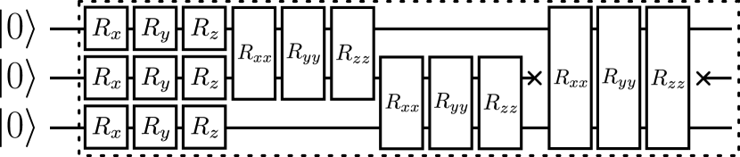
(a)  Parameterized unitary

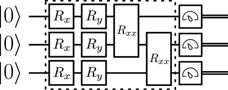
(b)  Parameterized quantum circuit Born machine

Figure 2: (a) A three-qubit example of the parameterized unitary used in the purification ansatz and the eigenvector creation in the convex-combination ansatz. The two-qubit gates for a chain act on qubits $i$ and $i+1$. The two-qubit gates also act on first and last qubit within a layer. (b) A three-qubit example of the parameterized quantum circuit Born machine that generates the probability distribution used in the convex-combination ansatz. The circuit elements within the dotted box form a layer, and each layer is repeated multiple times, depending on the problem instance. $\{R_{i}\}_{i\in\{x,y,z\}}$ denotes a single-qubit parameterized rotation about the axis $i$. Similarly $\{R_{i}\}_{i\in\{xx,yy,zz\}}$ are two-qubit parameterized rotations that can be used to generate entanglement.

In this section, we discuss the results of simulations of the QSlack algorithm for the example problems from Section II.3. We first discuss the common features to all the experiments and then delve into specifics for each example.

II.4.1 Input models

We begin by discussing the input models to the QSlack example problems. For the normalized trace distance, fidelity, and entanglement negativity, the inputs to the problem are quantum states. We generate mixed states as inputs for these problems using either the purification ansatz or the convex-combination ansatz (see Appendix D).

For the purification ansatz, following Appendix D.1, we pick the parameterized unitary to be of the form shown in Figure 2(a). The size of the purifying subsystem $R$, is chosen to be equal to that of the system of interest $S$, leading to a full-rank state on subsystem $S$. The parameters, i.e., the rotation angles, of the unitary operator are chosen at random. For all the parameterized unitaries, we fix the number of layers to be two.

For the convex-combination ansatz, following Appendix D.2, we use the same structure as the purification ansatz, as depicted in Figure 2(a), for the parameterized unitary $U(\gamma)$. To generate probabilities $p_{\varphi}$, we use a quantum circuit Born machine with the structure shown in Figure 2(b). The size of the quantum circuit Born machine is chosen to be equal to that of system $S$. The number of layers for all parameterized unitaries can be chosen arbitrarily, and in this work, we pick the number of layers to be two.

Lastly, for the constrained Hamiltonian optimization, the input to the problem is a Hermitian operator. As discussed in Section II.3.4, we use the Pauli input model from Appendix C.3.

Throughout training, we have sample access to the density matrices and probability distributions, through the purifying parameterized unitaries and measurement outcomes of the relevant quantum circuit Born machines.

II.4.2 Training

Similar to the inputs just discussed, we use either the purification or convex-combination ansatz to parameterize the density matrices being optimized. These density matrices are indeed optimization variables and unlike the input density matrices, the parameters are not held fixed. Training involves attempting to find optimal parameters that extremize the objective function value. In this work, we pick the form of the parameterized quantum states to be the same as the form of the input. For example, if the input to the trace-distance problem is two density matrices specified using a purification or convex-combination ansatz, then we pick the optimization variable to be of the same form.

At each iteration, the training process crucially depends on gradient estimation to pick the next set of parameters. While several algorithms can be employed for gradient estimation, we rely on the Simultaneous Perturbation Stochastic Approximation (SPSA) method [122] to estimate gradients. SPSA produces an unbiased estimator of the gradient with runtime constant in the number of parameters. Details of the method can be found in Appendix F.3. We use a maximum number of iterations as the stopping condition for all simulations.

The hyperparameters, like the learning rate and perturbation parameter, are tailored to each problem instance. We pick the smallest possible penalty parameter $c$ that suffices to enforce the constraints of the problem. This leads to faster convergence to the optimal value in practice.

	Purification ansatz	Convex-combination ansatz
1. Trace distance
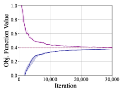
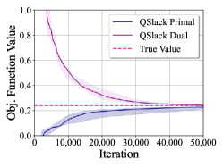
2. Fidelity
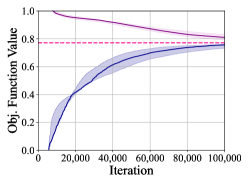
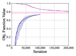
3. Negativity
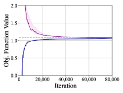
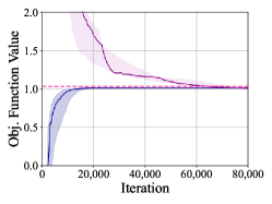
4. Constrained Hamiltonian

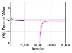
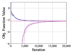
Figure 3: Convergence of both the primal and dual optimizations to their optimal values for various QSlack example problems. We used both the purification and convex-combination ansätze for each problem. The solid line shows the median value of the estimate, the shaded region represents the interquartile range, while the ground truth is marked by the dashed line. The number of runs over which the median and interquartile range are computed is ten for trace distance, four for root fidelity, and five for all others. Specific details regarding the runs, including the number of qubits, layers, gradient method, etc., can be found in Appendix H.

Prior to training, some of the parameters are initialized to specific values while others are set randomly. The initial parameter values of all parameterized quantum circuits are chosen uniformly at random from $[0,2\pi]$. For the normalized trace distance problem, in both the dual and the primal (see Propositions 12 and 13), parameters $\lambda$ and $\mu$ are initialized to one. For the root fidelity simulations, we initialize $\lambda$ to one and all components of vector $\left(\alpha_{\overrightarrow{x}}\right)_{\overrightarrow{x}}$ to zero in (32). Since the system size in our examples is relatively small, we include all components of the vectors in our training, instead of truncating to a polynomial number of them. We initialize to $\lambda=\mu=\nu=1$ in (34). For the entanglement negativity problem, parameters $\lambda$ and $\mu$ in (46) and (49) are initialized to one. The components of vectors $\alpha_{\overrightarrow{x_{A}},\overrightarrow{x_{B}}}$ and $\beta_{\overrightarrow{x_{A}},\overrightarrow{x_{B}}}$ are all initialized to zero. Similar to root fidelity, we include all components of these vectors in our training. Lastly for the constrained Hamiltonian optimization, we initialize to $y_{1}=y_{2}=\nu=0.001,\ \mu=-0.005$ in (466), and $z_{1}=0.1,\ z_{2}=0.5$ in (460).

II.4.3 Results

We used a noiseless simulator for the experiments in this work. However, we used the destructive swap test to estimate terms of the form $\operatorname{Tr}[\rho\sigma]$, which involves Bell measurements. Thus, estimates of the different terms involve sampling noise (also called shot noise). We leave the simulations of the different problems with other noise models to future work.

The plots for the various examples using both ansatz types are given in Figure 3. In these plots, we show the median (in solid lines) and interquartile range (in shading) of the objective function values over the course of training. The variation in objective function values across different runs corresponds to three sources of randomness: the randomized initializations of all parametrized quantum circuits, the inherent randomness of the SPSA method for gradient estimation, and shot noise in quantum circuit measurements. For root fidelity, we performed simulations without shot noise. For all other problems, we took $10^{12}$ shots, and the error achieved was typically on the order of $10^{-2}$. Details and specifics are discussed in Appendix H, and there we also give plots for the error and penalty values across training.

The simulations were performed using both the Qiskit quantum software development kit from IBM [125] and the Qulacs library [119].

III CSlack background, algorithm, examples, and simulations

III.1 Background on linear programming

Linear programming can be understood as a special case of semi-definite programming in which the Hermitian matrices $A$ and $B$ are diagonal and the Hermiticity preserving superoperator $\Phi$ takes diagonal matrices to diagonal matrices. This is quite similar to how classical information theory can be understood as a special case of quantum information theory in which all density matrices are diagonal and all quantum channels take diagonal density matrices to diagonal density matrices. This observation is what we use to understand the connection between the QSlack and CSlack methods for variational quantum semi-definite programming and variational linear programming, respectively.

Given this observation, we provide a quick review of linear programming, keeping in mind that it is the special case in which “everything from Section II.1 is diagonal.” As such, Hilbert–Schmidt inner products reduce to standard vector inner products, and the action of a superoperator on a matrix reduces to usual matrix-vector multiplication. Fix $d_{1},d_{2}\in\mathbb{N}$. Let $a$ be a $d_{1}\times 1$ real vector, $b$ a $d_{2}\times 1$ real vector, and $\phi$ a $d_{2}\times d_{1}$ real matrix. A linear program is specified by the triple $(a,b,\phi)$ and is defined as the following optimization problem:

$$\alpha_{L}\coloneqq\sup_{x\geq 0}\left\{a^{T}x:\phi x\leq b\right\},$$ (67)

where the supremum optimization is over every $d_{1}\times 1$ real vector $x$ with non-negative entries (i.e., the notation $x\geq 0$ is shorthand for every entry of $x$ being non-negative). Furthermore, the inequality constraint $\phi x\leq b$ is shorthand for every entry of the vector $b-\phi x$ being non-negative. The optimization in (67) is called the primal LP, and a vector $x$ is primal feasible if $x\geq 0$ and $\phi x\leq b$. The dual optimization problem is as follows:

$$\beta_{L}\coloneqq\inf_{y\geq 0}\left\{b^{T}y:\phi^{T}y\geq a\right\},$$ (68)

where the infimum optimization is over every $d_{2}\times 1$ real vector $y$ with non-negative entries and $\phi^{T}$ is the matrix transpose of $\phi$. A vector $y$ is dual feasible if both $y\geq 0$ and $\phi^{T}y\geq a$.

Weak duality corresponds to the inequality

$$\alpha_{L}\leq\beta_{L},$$ (69)

and strong duality corresponds to the equality $\alpha_{L}=\beta_{L}$. Strong duality holds whenever Slater’s condition is satisfied, i.e., if there exists a primal feasible $x$ and a strictly dual feasible $y$ or if there exists a strictly primal feasible $x$ and a dual feasible $y$.

As before, and for similar reasons, we can introduce slack variables to transform the inequality constraints in (67) and (68) to equality constraints. That is, we have the following:

$$\alpha_{L} =\sup_{x,w\geq 0}\left\{a^{T}x:b-\phi x=w\right\},$$ (70)

$$\beta_{L} =\inf_{y,z\geq 0}\left\{b^{T}y:\phi^{T}y-a=z\right\},$$ (71)

where $w$ is a $d_{2}\times 1$ real vector and $z$ is a $d_{1}\times 1$ real vector. Finally, it is possible to transform the constrained optimizations to unconstrained optimizations by introducing penalty terms in the objective functions, as follows:

$$\alpha_{L}(c)\coloneqq\sup_{x,w\geq 0}\left\{a^{T}x-c\left\|b-\phi x-w\right\|_{2}^{2}\right\},$$ (72)

$$\beta_{L}(c)\coloneqq\inf_{y,z\geq 0}\left\{b^{T}y+c\left\|\phi^{T}y-a-z\right\|_{2}^{2}\right\},$$ (73)

where $c>0$ is a penalty constant and $\left\|s\right\|_{2}$ is the Euclidean norm of a vector $s$. Again, by standard reasoning [15, Proposition 5.2.1], we have that

$$\alpha_{L}=\lim_{c\rightarrow\infty}\alpha_{L}(c),\qquad\beta_{L}=\lim_{c\rightarrow\infty}\beta_{L}(c),$$ (74)

and we thus arrive at a method for approximating the optimal values $\alpha_{L}$ and $\beta_{L}$. The reductions from (67) to (72) and from (68) to (73) are indeed standard, but they constitute some of the core preliminary observations behind our CSlack method.

III.2 CSlack algorithm for variational linear programming

Now we turn to describing the CSlack algorithm for variational linear programming. The idea is conceptually similar to QSlack and can be thought of as the classical version of it. Indeed, as mentioned before, linear programs can be thought of as the classical version of semi-definite programs in which every object is a diagonal matrix. As such, it follows that the density matrices, parameterized states, and observables from the previous section can be replaced with diagonal density matrices, diagonal parameterized states, and diagonal observables, which are equivalent to probability distributions, parameterized probability distributions, and observable vectors, respectively. In what follows, our discussion of CSlack mirrors that of QSlack, and as such, it can be quickly skimmed if the ideas behind QSlack are already clear.

A key assumption of the CSlack algorithm is that the vectors $a$ and $b$ and the matrix $\phi$ correspond to efficiently measurable observable vectors, meaning that they can be efficiently estimated on quantum or probabilistic computers (we describe precisely what we mean here later on and we provide particular examples of efficiently measurable observable vectors and input models for $a$, $b$, and $\phi$ in Appendices C.5 and C.6). We assume that $d_{1}=2^{n}$ and $d_{2}=2^{m}$ for $n,m\in\mathbb{N}$, so that the entries of $a$ are indexed by $n$-bit strings and the entries of $b$ are indexed by $m$-bit strings. Thus, the vectors $a$ and $b$ and the matrix $\phi$ are exponentially large in the parameters $n$ and $m$.

A basic observation is that the vectors $x$, $w$, $y$, and $z$ appearing in the optimizations in (72)–(73) can be represented as scaled probability distributions. Whenever $x\neq 0$, it can be written as $x=\lambda r$, where $\lambda\coloneqq\boldsymbol{1}^{T}x$ and $r\coloneqq x/\lambda$, with $\boldsymbol{1}$ the vector of all ones, so that $\lambda>0$ and $r$ is a probability distribution on $2^{n}$ elements. We can thus write the optimizations in (72)–(73) as follows:

$$\alpha_{L}(c) =\sup_{\begin{subarray}{c}\lambda,\mu\geq 0,\\ r,s\in\mathcal{P}\end{subarray}}\left\{\lambda a^{T}r-c\left\|b-\lambda\phi r-\mu s\right\|_{2}^{2}\right\},$$ (75)

$$\beta_{L}(c) =\inf_{\begin{subarray}{c}\kappa,\nu\geq 0,\\ t,w\in\mathcal{P}\end{subarray}}\left\{\kappa b^{T}t+c\left\|\kappa\phi^{T}t-a-\nu w\right\|_{2}^{2}\right\},$$ (76)

where we have made the substitutions $x=\lambda r$, $w=\mu s$, $y=\kappa t$, and $z=\nu w$, and $\mathcal{P}$ denotes the set of all probability distributions. Here we are taking advantage of the structure of probability theory, namely, that probability distributions are described by vectors with non-negative entries, in order to impose the entrywise non-negative constraints on $x$, $w$, $y$, and $z$.

Expressions like $a^{T}r$ and $b^{T}t$ in (75)–(76) can be understood as expectations of the observable vectors $a$ and $b$ with respect to the probability distributions $r$ and $t$, respectively. That is, by labeling the $i$th entry of $a$ and $r$ as $a_{i}$ and $r_{i}$, respectively, we see that

$$a^{T}r=\sum_{i}r_{i}a_{i},$$ (77)

which is the equation for the expectation of a random variable taking the value $a_{i}$ with probability $r_{i}$. As such, the quantities $a^{T}r$ and $b^{T}t$ can be estimated through repetition, by repeatedly sampling from the probability distributions $r$ and $t$, performing the procedures to evaluate the entries of $a$ and $b$, and finally calculating sample means as estimates of $a^{T}r$ and $b^{T}t$. In Appendices C.5 and C.6, we discuss how the other terms $\left\|b-\lambda\phi r-\mu s\right\|_{2}^{2}$ and $\left\|\kappa\phi^{T}t-a-\nu w\right\|_{2}^{2}$ can be estimated, for which the collision test is helpful (i.e., the classical version of the swap test).

We have rewritten the objective functions in (72)–(73) as in (75)–(76), in terms of expectations of observable vectors. However, evaluating these is too difficult because the optimizations are over all possible probability distributions and not all probability distributions are efficiently preparable. Similar to QSlack, our next modification is to replace the optimizations over all possible probability distributions in (75)–(76) with optimizations over parameterized probability distributions that are efficiently preparable, leading to

$$\tilde{\alpha}_{L}(c) \coloneqq\Big{\{}\sup_{\lambda,\mu\geq 0,\theta_{1},\theta_{2}\in\Theta}\lambda a^{T}r(\theta_{1})$$

$$\qquad\qquad-c\left\|b-\lambda\phi r(\theta_{1})-\mu s(\theta_{2})\right\|_{2}^{2}\Big{\}},$$ (78)

$$\tilde{\beta}_{L}(c) \coloneqq\Big{\{}\inf_{\kappa,\nu\geq 0,\theta_{3},\theta_{4}\in\Theta}\kappa b^{T}t(\theta_{3})$$

$$\qquad\qquad+c\left\|\kappa\phi^{T}t(\theta_{3})-a-\nu w(\theta_{4})\right\|_{2}^{2}\Big{\}},$$ (79)

where $\Theta$ is a general set of all possible parameter vectors, $\theta_{1}$, $\theta_{2}$, $\theta_{3}$, and $\theta_{4}$ are vectors of parameter values, and $r(\theta_{1})$, $s(\theta_{2})$, $t(\theta_{3})$, and $w(\theta_{4})$ are parameterized probability distributions. Appendix D.2 discusses two methods for parameterizing the set of probability distributions, one based on neural-network generative models [6, 23, 95] and another based on Born machines [67, 32, 18], specifically, quantum circuit Born machines [18]. In the latter case, i.e., if a quantum generative model is used, it is worth noting that CSlack is still a quantum algorithm. A key aspect of all these methods is that one can efficiently sample from these parameterized probability distributions.

One could also consider using an explicit model to train the model probability distribution directly. Examples of such models include auto-regressive models [131], RNNs [110], tensor networks without loops (which includes tensor network Born machines) [67, 37]. While these models are in general less expressive they can be easier to train [109]. For the sake of brevity, we will not explore this possibility further here.

A benefit of the optimization problems in (78)–(79) is that all expressions in the objective functions in (78)–(79) are efficiently estimable by sampling. Additionally, the following inequalities hold:

$$\alpha_{L}(c) \geq\tilde{\alpha}_{L}(c),$$ (80)

$$\beta(c) \leq\tilde{\beta}_{L}(c),$$ (81)

because the set of parameterized probability distributions is a strict subset of all possible probability distributions. Then the ability to optimize $\tilde{\alpha}_{L}(c)$ and $\tilde{\beta}_{L}(c)$ for each $c>0$ implies the following theorem:

Theorem 2

The following inequalities hold

$$\tilde{\alpha}_{L}\leq\alpha_{L}\leq\beta_{L}\leq\tilde{\beta}_{L},$$ (82)

where $\alpha_{L}$ and $\beta_{L}$ are defined in (67)–(68),

$$\tilde{\alpha}_{L} \coloneqq\sup_{\begin{subarray}{c}\lambda,\mu\geq 0,\\ \theta_{1},\theta_{2}\in\Theta\end{subarray}}\left\{\lambda a^{T}r(\theta_{1}):b-\lambda\phi r(\theta_{1})=\mu s(\theta_{2})\right\},$$ (83)

$$\tilde{\beta}_{L} \coloneqq\inf_{\begin{subarray}{c}\kappa,\nu\geq 0,\\ \theta_{3},\theta_{4}\in\Theta\end{subarray}}\left\{\lambda b^{T}t(\theta_{3}):\kappa\phi^{T}t(\theta_{3})-a=\nu w(\theta_{4})\right\},$$ (84)

$a$ is a $2^{n}\times 1$ real vector, $b$ is a $2^{m}\times 1$ real vector, $\phi$ is a $2^{m}\times 2^{n}$ real matrix, and $\Theta$ is a general set of parameter vectors.

Proof. The conclusion in (82) follows from (69), (74), (80)–(81), and $\lim_{c\rightarrow\infty}\tilde{\alpha}_{L}(c)=\tilde{\alpha}_{L}$ and $\lim_{c\rightarrow\infty}\tilde{\beta}_{L}(c)=\tilde{\beta}_{L}$, which both follow from [15, Proposition 5.2.1].   

Mirroring Eq. (19) for QSlack, Eq. (82) is a key theoretical insight for the CSlack method. Under the assumptions that $a$, $b$, and $\phi$ correspond to efficiently measurable observable vectors, in principle, we can sandwich the optimal values of the LPs in (67)–(68) by optimization problems whose objective functions are efficiently estimable. One could then attempt to optimize $\tilde{\alpha}_{L}(c)$ and $\tilde{\beta}_{L}(c)$ for a sequence of penalties, following the standard approach of the penalty method.

As with QSlack and other optimization problems involving generative models, the main drawback of CSlack is that the optimizations in (75)–(76) over the convex set of probability distributions are now replaced with the optimizations in (78)–(79) over the non-convex set of parameterized probability distributions. Given this, even though the optimizations are over fewer parameters, their landscapes feature local minima that can make convergence to global optima difficult.

To optimize the objective function in (79), we employ an approach that involves using a probabilistic or quantum computer to evaluate quantities like $b^{T}t(\theta_{3})$, by means of sampling and repetition, as well as other terms in the objective function like $a^{T}w(\theta_{4})$, which arises as one of the six terms after expanding $\left\|\kappa\phi^{T}t(\theta_{3})-a-\nu w(\theta_{4})\right\|_{2}^{2}$. After doing so, we can employ gradient descent or other related algorithms to determine a new choice of the parameters $\theta_{3}$ and $\theta_{4}$; then we iterate this process until either convergence occurs or after a specified maximum number of iterations. One can follow a similar route for the optimization problem in (78).

In order to execute the CSlack method, we also require estimating the gradient vectors of the objective functions in (78)–(79). For a quantum circuit Born machine, one can again do so by means of a parameter-shift rule [81]. For generative models, one can use the simultaneous perturbation stochastic approximation [122] to estimate gradients.

In summary, the main idea of CSlack is similar to that of QSlack: replace the original LPs in (67)–(68) with a sequence of optimizations of the form in (78) and (79), respectively. The main advantage of CSlack is that every term in the objective functions of (78) and (79), as well as their gradients, are efficiently estimable on quantum or probabilistic computers. Furthermore, the inequalities in (82) provide theoretical guarantees that, if one can calculate the optimal values in (78) and (79) for each $c>0$, then the resulting quantities $\tilde{\alpha}_{L}$ and $\tilde{\beta}_{L}$ are certified bounds on the true optimal values $\alpha_{L}$ and $\beta_{L}$, thus sandwiching the true optimal values. The main drawback of CSlack is that the reformulation involves an optimization over the non-convex set of parameterized probability distributions, but this aspect is common to all classical variational or neural network methods.

III.3 CSlack example problems

In this section, we present a variety of CSlack example problems relevant for information theory and physics, including the following:

1. total variation distance, the classical version of the normalized trace distance,

2. and constrained classical Hamiltonian optimization, in which the Hamiltonian and constraints are all diagonal in the computational basis.

For problem 1, we assume that one has sample access to the probability distribution, so that the input model here is the linear combination of distributions input model, as described in Appendix C.5. That is, there is some procedure, whether it be by a probabilistic circuit or other means, that prepares the distributions and can be repeated in such a way that the same state is prepared each time. For example, if the distribution to be prepared is $p$, we assume that there is a procedure to prepare $p^{\otimes n}$ for $n\in\mathbb{N}$ arbitrarily large. For problem 2, the Walsh–Hadamard input model is quite natural and so we consider this in our example below (see Appendix C.6 for more details).

III.3.1 Total variation distance

We now move on to some example problems for CSlack, beginning with the total variation distance of two probability distributions. This is the classical version of the problem studied in Section II.3.1, and as such, it is obtained easily from it by requiring that all of the density matrices therein are diagonal. Nevertheless, we briefly summarize the problem here for completeness.

For probability distributions $p$ and $q$ over $n$ bits (i.e., $2^{n}$-dimensional probability vectors), the total variation distance is defined as follows:

$$\frac{1}{2}\left\|p-q\right\|_{1} =\sup_{t\geq 0}\left\{t^{T}\left(p-q\right):t\leq\boldsymbol{1}\right\},$$ (85)

$$=\inf_{y\geq 0}\left\{\boldsymbol{1}^{T}y:y\geq p-q\right\},$$ (86)

where $\left\|\cdot\right\|_{1}$ denotes the $\ell_{1}$ vector norm, $t$ and $y$ are $2^{n}$-dimensional vectors, $\boldsymbol{1}$ is a $2^{n}$-dimensional vector of all ones, and the inequalities have the meaning discussed after (67). The primal and dual SDPs in (85)–(86) follow directly by plugging in diagonal density matrices into (26)–(27). Since $p-q$ appears in the primal and dual optimizations, the input model for this problem is the linear combination of distributions model, as discussed in Appendix C.5. Since the optimizations above are over $2^{n}$-dimensional vectors $t$ and $y$, subject to the constraints above, it is not possible to estimate $\frac{1}{2}\left\|p-q\right\|_{1}$ efficiently using standard LP solvers.

If $p$ and $q$ are prepared by circuits with access to randomness, it is known that a decision problem related to estimating their total variation distance is SZK-complete [124], which indicates that the worst-case complexity of this problem is considered intractable for a probabilistic classical computer (and also for a quantum computer). Regardless, we can attempt to estimate this quantity by means of the CSlack method.

Focusing on the dual optimization in (86), we can rewrite it exactly as follows:

$$\inf_{y\geq 0}\left\{\boldsymbol{1}^{T}y:y\geq p-q\right\}\\ =\lim_{c\rightarrow\infty}\inf_{\begin{subarray}{c}\lambda,\mu\geq 0,\\ r,s\in\mathcal{P}\end{subarray}}\left\{\lambda+c\left\|\lambda r-p+q-\mu s\right\|_{2}^{2}\right\}.$$ (87)

This follows directly from plugging diagonal density matrices into (28). As outlined in (78)–(79), we replace the optimizations over all probability distributions $r,s\in\mathcal{P}$ with optimizations over parameterized distributions, using either a generative model or a quantum circuit Born machine. The $\ell_{2}$ norm in (87) can be expanded into ten different overlap terms, and each of them can be estimated efficiently using the collision test (i.e., classical version of swap test), reviewed in Appendix C.5.

III.3.2 Constrained classical Hamiltonian optimization

The constrained classical Hamiltonian optimization problem is similar to that detailed in Section II.3.4, with the exception that all matrices involved are diagonal, and as such, they can be represented as classical vectors. For completeness, we go through the problem briefly here.

The inputs to this problem are a real Hamiltonian vector $h$ and $\ell$ real constraint vectors $a_{1},\ldots,a_{\ell}$, as well as real constraint numbers $b_{1},\ldots,b_{\ell}$. We further suppose that $h$, $a_{1},\ldots,a_{\ell}$ are efficiently measurable vectors. Then the classical constrained Hamiltonian optimization problem is as follows:

$$\mathcal{L}(h,a_{1},\ldots,a_{\ell})$$

$$\coloneqq\inf_{p\in\mathcal{P}}\left\{h^{T}p:a_{i}^{T}p\geq b_{i}\text{ }\forall i\in\left[\ell\right]\right\}$$ (88)

$$=\sup_{\begin{subarray}{c}y_{1},\ldots,y_{\ell}\geq 0,\\ \mu\in\mathbb{R}\end{subarray}}\left\{\sum_{i=1}^{\ell}b_{i}y_{i}+\mu:\sum_{i=1}^{\ell}y_{i}a_{i}+\mu\boldsymbol{1}\leq h\right\},$$ (89)

where we have written the dual LP in (89). Furthermore, the classical ground-state energy problem is a special case with $a_{i}=0$ and $b_{i}=0$ for all $i\in\left[\ell\right]$, leading to

$$\mathcal{L}(h) \coloneqq\inf_{p\in\mathcal{P}}\left\{h^{T}p\right\}$$

$$=\sup_{\mu\in\mathbb{R}}\left\{\mu:\mu\boldsymbol{1}\leq h\right\}.$$ (90)

A natural input model for this problem is the Walsh–Hadamard input model, described further in Appendix C.6, such that

$$h =\sum_{\overrightarrow{x}}h_{\overrightarrow{x}}s_{\overrightarrow{x}},$$ (91)

$$a_{i} =\sum_{\overrightarrow{x}}a_{\overrightarrow{x}}^{i}s_{\overrightarrow{x}}\qquad\forall i\in\left[\ell\right],$$ (92)

where $h_{\overrightarrow{x}},a_{\overrightarrow{x}}^{1},\ldots,a_{\overrightarrow{x}}^{\ell}\in\mathbb{R}$ for all $\overrightarrow{x}$ and $s_{\overrightarrow{x}}$ is a Walsh–Hadamard vector, i.e.,

$$s_{\overrightarrow{x}}\coloneqq s_{x_{1}}\otimes\cdots\otimes s_{x_{n}},$$ (93)

$$s_{0}\coloneqq\begin{bmatrix}1\\ 1\end{bmatrix},\qquad s_{1}\coloneqq\begin{bmatrix}1\\ -1\end{bmatrix}.$$ (94)

Observe that $s_{0}$ and $s_{1}$ are the diagonal entries of the diagonal Pauli matrices $\sigma_{I}$ and $\sigma_{Z}$. Using this approach, we can again rewrite the primal and dual optimization problems as in (59) and (65), respectively, with the only substitutions being as follows:

$$\operatorname{Tr}[\sigma_{\overrightarrow{x}}\rho] \rightarrow s_{\overrightarrow{x}}^{T}p,$$ (95)

$$\operatorname{Tr}[\omega^{2}] \rightarrow w^{T}w,$$ (96)

$$\operatorname{Tr}[\sigma_{\overrightarrow{x}}\omega] \rightarrow s_{\overrightarrow{x}}^{T}w,$$ (97)

where $w$ is a probability distribution. Each of the inner products above can be estimated by sampling, as discussed in Appendix C.6.

In general, the vectors $\left(h_{\overrightarrow{x}}\right)_{\overrightarrow{x}},\left(a_{\overrightarrow{x}}^{1}\right)_{\overrightarrow{x}},\ldots,\left(a_{\overrightarrow{x}}^{\ell}\right)_{\overrightarrow{x}}$ each have $2^{n}$ coefficients. However, for problems of physical interest, in which the Hamiltonians and constraints consist of few-body interactions, there are only poly$(n)$ non-zero coefficients in these vectors. In order to be able to evaluate the modified objective functions efficiently, we restrict the optimizations over the probability distributions $p$ and $w$ to be over parameterized probability distributions.

III.4 CSlack simulations

In this section, we report the results of simulations of the CSlack algorithm for the example problems from Section III.3. We first discuss the features common to all experiments and then delve into specifics for each example.

III.4.1 Input models

Let us begin by discussing the input models to the CSlack example problems. For total variation distance, the inputs to the problem are two probability distributions. These distributions are generated using distinct two-layer quantum circuit Born machines with randomly set parameters (see Appendix D.2). The input to the constrained classical Hamiltonian optimization is a vector operator, decomposed in the Walsh–Hadamard basis (see Appendix C.6).

III.4.2 Training

Similar to QSlack, at each iteration, the training process crucially depends on gradient estimation to pick the next set of parameters. We use the SPSA method to produce an unbiased estimator of the gradient with runtime constant in the number of parameters. Details of the method can be found in Appendix F.3. We use a maximum number of iterations as the stopping condition for all simulations.

Similarly, the hyperparameters, like the learning rate and perturbation parameter, are tailored to each problem instance. We pick the smallest possible penalty parameter $c$ that suffices to enforce the constraints of the problem. This leads to faster convergence to the optimal value in practice. Details and specifics are discussed in Appendix H.

Similar to the QSlack simulations, the initial parameters of all quantum circuit Born machines are chosen uniformly at random from $[0,2\pi]$. For the total variation distance problem, the parameters $\lambda$ and $\mu$ in (87) are initialized to one. For the constrained classical Hamiltonian optimization, parameters $y_{1},\ldots,y_{\ell}$ and $\mu$ in (89) are all initialized to zero.

III.4.3 Results

We used a noiseless simulator for the experiments in this work. The collision test involves sampling, leading to the estimate being affected by shot noise. We leave the simulations of the different problems with other noise models to future work.

The plots for the various examples using both ansatz types are given in Figures 4 and 5. In these plots, we show the median (in solid lines) and interquartile range (in shading) of the objective function values over the course of training. The variation in objective function values across different runs corresponds to three sources of randomness: the randomized initializations of all parametrized quantum circuits, the inherent randomness of the SPSA method for gradient estimation, and shot noise in quantum circuit measurements. For all problems, we took $10^{12}$ shots, and the error achieved was typically on the order of $10^{-2}$.

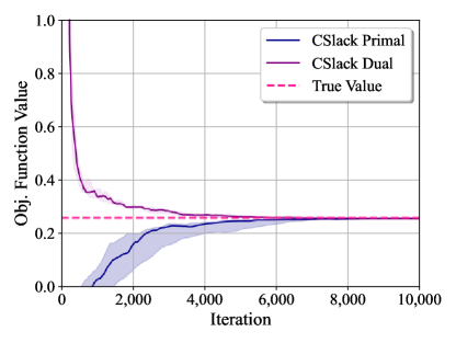
Figure 4: Convergence of the CSlack method for total variation distance, from both above and below across ten runs. Specific details regarding the runs, including the number of qubits, layers, gradient method, etc., can be found in Appendix H.

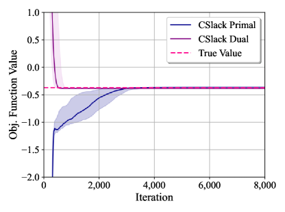
Figure 5: Convergence of the CSlack method for the constrained classical Hamiltonian optimization, from both above and below across ten runs. Specific details regarding the runs, including the particular Hamiltonian choice, gradient method, etc., can be found in Appendix H.

IV Conclusion

In summary, we proposed the QSlack and CSlack methods as general approaches for estimating upper and lower bounds on the optimal values of semi-definite and linear programs, respectively. The methods consist of the following steps: 1) replace inequality constraints with equality constraints via the introduction of slack variables, 2) replace a constrained optimization with an unconstrained one by means of the penalty method, using the Hilbert–Schmidt distance for SDPs and the Euclidean distance for LPs, 3) replace optimizations over non-negative variables with either scaled density matrices or scaled probability distributions, and 4) replace optimizations over density matrices or probability distributions with parameterized ones. Then we estimate all terms in the objective functions by means of sampling, using a quantum computer in the SDP case and a probabilistic or quantum computer for the LP case. If it is possible to optimize the objective functions, then it follows that the QSlack and CSlack methods give certified upper and lower bounds on the true optimal values in the limit $c\rightarrow\infty$.

We considered a variety of example problems in Section II.3, which showcase the variety of problems and input models that the QSlack and CSlack methods can handle. Examples for QSlack include estimating normalized trace distance, root fidelity, and entanglement negativity, problems of interest in quantum information science, as well as constrained Hamiltonian optimization, a problem of interest in physics and chemistry. Examples for CSlack include estimating total variation distance and classical constrained Hamiltonian optimization. In our numerical simulations, we found that both the primal and dual optimizations for each problem approach the true value, achieving errors typically on the order of $10^{-2}$.

Going forward from here, there a number of open directions to consider. First, the behavior of QSlack for finite $c$ values warrants a more detailed study. Our numerics suggest that in general QSlack provides genuine bounds even for finite $c$; however, as expected, occasional deviations are observed. It would be valuable to investigate whether it is possible to obtain bounds on the degree to which deviations are possible for finite $c$. Such bounds would allow one to certify the degree of confidence one may have in the outputs of QSlack and hence guide one’s choice for the value of $c$.

Longer term, we would like to scale up our simulations and examples to include many more qubits, in order to have a sense of the scaling of QSlack and CSlack. Indeed, these methods are intended to apply to large-scale optimization problems, beyond the reach of what is possible classically. In scaling up, it will be necessary to incorporate error mitigation [31], in order to reduce the impact of noise. Additionally, when scaling up, it is inevitable that the issue of barren plateaus [87] will come into play, in which higher depth quantum circuits are expected to have vanishing gradients and vanishing cost differences [3]. This occurs for highly expressive [66] or highly entangling [90] ansätze and even at low depths for global costs [35]. In Appendix I, we discuss the cases for which QSlack can or cannot potentially avoid barren plateaus.

We note that while we have here largely presented QSlack as a variational quantum algorithm, the parametrized unitary could in theory take other forms. For example, for low entangling models, one could use a tensor-network based optimization. Or, more generally, one could envision complementing classical simulation methods supported with data obtained from a quantum computer [16, 69, 107]. This would be an interesting avenue to explore should the barrier presented by barren plateaus prove insurmountable.

As another open direction, we also wonder whether QSlack could be modified generally to become an interior-point method, which is the standard approach to solving SDPs and LPs on classical computers (we observed one case in (64) in which it can be). The main question here is whether it is possible to rewrite the penalty terms in (13)–(14) as self-concordant barrier functions [97, Section 5.4.6] that could be efficiently estimated on quantum computers. The main advantage of QSlack is that all terms in the objective functions in (13)–(14) can be evaluated efficiently on quantum computers, but the Hilbert–Schmidt norm is not a self-concordant barrier function. The logarithm of the determinant of a matrix is known to be a self-concordant barrier function for the cone of positive semi-definite matrices. As such, finding a way to generalize the classical sampling approach of [14] to the quantum case would be helpful in modifying QSlack to become an interior-point method.

Data availability statement—All software codes used to run the simulations and generate the figures in this paper and in our companion paper [140] are available as arXiv ancillary files with the arXiv posting of this paper.

Appendix A Alternative penalty method optimizations

In (10)–(11), we proposed unconstrained optimization problems $\alpha(c)$ and $\beta(c)$ that each converge to $\alpha$ and $\beta$, respectively, in the limit as $c\rightarrow\infty$. While these quantities are the main focus of our paper, here we propose some variants of these quantities that still have the property that they converge to $\alpha$ and $\beta$ in the limit as $c\rightarrow\infty$, while they are also concave and convex optimization problems, respectively, and obey a weak-duality inequality. They are defined as follows for $c>0$, $p_{1},p_{2}\geq 1$, with $q_{i}$ chosen such that $\frac{1}{p_{i}}+\frac{1}{q_{i}}=1$, for $i\in\left\{1,2\right\}$:

$$\alpha_{p_{1},q_{2}}^{\prime}(c) \coloneqq\sup_{X,W\geq 0}\left\{\operatorname{Tr}[AX]-c\left\|B-\Phi(X)-W\right\|_{p_{1}}:\left\|X\right\|_{q_{2}}\leq c\right\},$$ (98)

$$\beta_{p_{2},q_{1}}^{\prime}(c) \coloneqq\inf_{Y,Z\geq 0}\left\{\operatorname{Tr}\!\left[BY\right]+c\left\|\Phi^{{\dagger}}(Y)-A-Z\right\|_{p_{2}}:\left\|Y\right\|_{q_{1}}\leq c\right\},$$ (99)

where the Schatten $p$-norm of an operator $M$ is defined for $p\geq 1$ as

$$\left\|M\right\|_{p}\coloneqq\left(\operatorname{Tr}\!\left[\left|M\right|^{p}\right]\right)^{1/p},$$ (100)

with $\left|M\right|\coloneqq\sqrt{M^{{\dagger}}M}$. The main difference between these quantities and those in (10)–(11) are that their penalty terms do not feature the square and they have the additional constraints $\left\|X\right\|_{q_{2}}\leq c$ and $\left\|Y\right\|_{q_{1}}\leq c$. As an example, we could choose $p_{i}=1$ and $q_{i}=\infty$ for $i\in\left\{1,2\right\}$, leading to the optimizations:

$$\alpha_{1,\infty}^{\prime}(c) \coloneqq\sup_{X,W\geq 0}\left\{\operatorname{Tr}[AX]-c\left\|B-\Phi(X)-W\right\|_{1}:\left\|X\right\|_{\infty}\leq c\right\},$$ (101)

$$\beta_{1,\infty}^{\prime}(c) \coloneqq\inf_{Y,Z\geq 0}\left\{\operatorname{Tr}\!\left[BY\right]+c\left\|\Phi^{{\dagger}}(Y)-A-Z\right\|_{1}:\left\|Y\right\|_{\infty}\leq c\right\},$$ (102)

which are rather natural choices if $X$ and $Y$ are observables and $W$ and $Z$ are states, along with the linear combination of states model from Appendix C.2. Another natural choice, strongly related to the choices made in the main text in (10)–(11), is when $p_{i}=q_{i}=2$ for $i\in\left\{1,2\right\}$, leading to

$$\alpha_{2,2}^{\prime}(c) \coloneqq\sup_{X,W\geq 0}\left\{\operatorname{Tr}[AX]-c\left\|B-\Phi(X)-W\right\|_{2}:\left\|X\right\|_{2}\leq c\right\},$$ (103)

$$\beta_{2,2}^{\prime}(c) \coloneqq\inf_{Y,Z\geq 0}\left\{\operatorname{Tr}\!\left[BY\right]+c\left\|\Phi^{{\dagger}}(Y)-A-Z\right\|_{2}:\left\|Y\right\|_{2}\leq c\right\},$$ (104)

such that every operator and constraint are measured with respect to the Hilbert–Schmidt norm or distance.

Proposition 3

Let $p_{1},p_{2}\geq 1$, with $q_{i}$ chosen such that $\frac{1}{p_{i}}+\frac{1}{q_{i}}=1$, for $i\in\left\{1,2\right\}$. Then the optimization problem $\alpha_{p_{1},q_{2}}^{\prime}(c)$ is concave, and the optimization problem $\beta_{p_{2},q_{1}}^{\prime}(c)$ is convex.

Proof. Let $X_{i},W_{i}\geq 0$ be such that $\left\|X_{i}\right\|_{q_{2}}\leq c$ for $i\in\left\{0,1\right\}$, and let

$$\lambda \in\left[0,1\right],$$ (105)

$$X_{\lambda} \coloneqq\left(1-\lambda\right)X_{0}+\lambda X_{1},$$ (106)

$$W_{\lambda} \coloneqq\left(1-\lambda\right)W_{0}+\lambda W_{1}.$$ (107)

Then

$$\operatorname{Tr}[AX_{\lambda}]-c\left\|B-\Phi(X_{\lambda})-W_{\lambda}\right\|_{p_{1}}\geq\left(1-\lambda\right)\left(\operatorname{Tr}[AX_{0}]-c\left\|B-\Phi(X_{0})-W_{0}\right\|_{p_{1}}\right)\\ +\lambda\left(\operatorname{Tr}[AX_{1}]-c\left\|B-\Phi(X_{1})-W_{1}\right\|_{p_{1}}\right),$$ (108)

which follows from linearity of the superoperator $\Phi$ and convexity of the norm $\left\|\cdot\right\|_{p_{1}}$. Furthermore, due to convexity of the norm $\left\|\cdot\right\|_{q_{2}}$, it follows that $\left\|X_{\lambda}\right\|_{q_{2}}\leq c$. Thus, the claim about $\alpha_{p_{1},q_{2}}^{\prime}(c)$ follows. A similar argument implies that $\beta_{p_{2},q_{1}}^{\prime}(c)$ is a convex optimization problem.   

An additional feature of these optimization problems is that the weak-duality inequality $\alpha_{p_{1},q_{2}}^{\prime}(c)\leq\beta_{p_{2},q_{1}}^{\prime}(c)$ holds for every $c>0$. To establish this claim, we begin with the following lemma:

Lemma 4

Let $X,W,Y,Z\geq 0$, let $A$ and $B$ be Hermitian matrices, and let $\Phi$ be a Hermiticity-preserving superoperator. Then

$$\operatorname{Tr}[AX]-\left\|Y\right\|_{q_{1}}\left\|B-\Phi(X)-W\right\|_{p_{1}}\leq\operatorname{Tr}\!\left[BY\right]+\left\|X\right\|_{q_{2}}\left\|\Phi^{{\dagger}}(Y)-A-Z\right\|_{p_{2}},$$ (109)

where $p_{1},p_{2}\geq 1$ and $q_{i}$ is chosen such that $\frac{1}{p_{i}}+\frac{1}{q_{i}}=1$, for $i\in\left\{1,2\right\}$.

Proof. The idea is to proceed by means of an approximate version of the standard proof of the weak-duality inequality (see, e.g., [72, Proposition 2.21]). Set

$$\varepsilon_{1}(X,W) \coloneqq\left\|B-\Phi(X)-W\right\|_{p_{1}},$$ (110)

$$\varepsilon_{2}(Y,Z) \coloneqq\left\|\Phi^{{\dagger}}(Y)-A-Z\right\|_{p_{2}}.$$ (111)

Recall the following variational characterizations of the Schatten norms (see, e.g., [72, Proposition 2.11]):

$$\varepsilon_{1}(X,W) =\sup_{W^{\prime}}\left\{\left|\left\langle B-\Phi(X)-W,W^{\prime}\right\rangle\right|:\left\|W^{\prime}\right\|_{q_{1}}\leq 1\right\}$$ (112)

$$=\sup_{W^{\prime}}\left\{\left|\left\langle B-W,W^{\prime}\right\rangle-\left\langle\Phi(X),W^{\prime}\right\rangle\right|:\left\|W^{\prime}\right\|_{q_{1}}\leq 1\right\},$$ (113)

$$\varepsilon_{2}(Y,Z) =\sup_{Z^{\prime}}\left\{\left|\left\langle\Phi^{{\dagger}}(Y)-A-Z,Z^{\prime}\right\rangle\right|:\left\|Z^{\prime}\right\|_{q_{2}}\leq 1\right\}$$ (114)

$$=\sup_{Z^{\prime}}\left\{\left|\left\langle\Phi^{{\dagger}}(Y)-Z,Z^{\prime}\right\rangle-\left\langle A,Z^{\prime}\right\rangle\right|:\left\|Z^{\prime}\right\|_{q_{2}}\leq 1\right\}.$$ (115)

Now consider that

$$\operatorname{Tr}[AX] \leq\operatorname{Tr}\!\left[\left(\Phi^{{\dagger}}(Y)-Z\right)X\right]+\left\|X\right\|_{q_{2}}\varepsilon_{2}(Y,Z)$$ (116)

$$\leq\operatorname{Tr}\!\left[\Phi^{{\dagger}}(Y)X\right]+\left\|X\right\|_{q_{2}}\varepsilon_{2}(Y,Z)$$ (117)

$$=\operatorname{Tr}\!\left[Y\Phi(X)\right]+\left\|X\right\|_{q_{2}}\varepsilon_{2}(Y,Z)$$ (118)

$$\leq\operatorname{Tr}\!\left[Y\left(B-W\right)\right]+\left\|Y\right\|_{q_{1}}\varepsilon_{1}(X,W)+\left\|X\right\|_{q_{2}}\varepsilon_{2}(Y,Z)$$ (119)

$$\leq\operatorname{Tr}\!\left[BY\right]+\left\|Y\right\|_{q_{1}}\varepsilon_{1}(X,W)+\left\|X\right\|_{q_{2}}\varepsilon_{2}(Y,Z).$$ (120)

The first inequality follows because

$$\operatorname{Tr}[AZ^{\prime}]\leq\operatorname{Tr}\!\left[\left(\Phi^{{\dagger}}(Y)-Z\right)Z^{\prime}\right]+\left\|Z^{\prime}\right\|_{q_{2}}\varepsilon_{2}(Y,Z)$$ (121)

for every Hermitian $Z^{\prime}$, as a consequence of (115). The second inequality follows because $\operatorname{Tr}[ZX]\geq 0$, given that $X,Z\geq 0$. The third inequality follows because

$$\operatorname{Tr}\!\left[W^{\prime}\Phi(X)\right]\leq\operatorname{Tr}\!\left[W^{\prime}\left(B-W\right)\right]+\left\|W^{\prime}\right\|_{q_{1}}\varepsilon_{1}(X,W)$$ (122)

for every Hermitian $W^{\prime}$, as a consequence of (113). The final inequality follows because $\operatorname{Tr}[YW]\geq 0$, since $Y,W\geq 0$. This implies that the following inequality holds for all $X,W,Y,Z\geq 0$:

$$\operatorname{Tr}[AX]-\left\|Y\right\|_{q_{1}}\varepsilon_{1}(X,W)\leq\operatorname{Tr}\!\left[BY\right]+\left\|X\right\|_{q_{2}}\varepsilon_{2}(Y,Z),$$ (123)

or equivalently, that the following holds for all $X,W,Y,Z\geq 0$:

$$\operatorname{Tr}[AX]-\left\|Y\right\|_{q_{1}}\left\|B-\Phi(X)-W\right\|_{p_{1}}\leq\operatorname{Tr}\!\left[BY\right]+\left\|X\right\|_{q_{2}}\left\|\Phi^{{\dagger}}(Y)-A-Z\right\|_{p_{2}}.$$ (124)

This concludes the proof.   

Thus, if there is a uniform upper bound $c\geq\max\{\left\|X\right\|_{q_{2}},\left\|Y\right\|_{q_{1}}\}$ holding for every $X\geq 0$ and $Y\geq 0$ under consideration, then the following inequality holds

$$\operatorname{Tr}[AX]-c\left\|B-\Phi(X)-W\right\|_{p_{1}}\leq\operatorname{Tr}\!\left[BY\right]+c\left\|\Phi^{{\dagger}}(Y)-A-Z\right\|_{p_{2}},$$ (125)

That is, we have the following corollary:

Corollary 5

Let $A$ and $B$ be Hermitian matrices, and let $\Phi$ be a Hermiticity-preserving superoperator. Let $p_{1},p_{2}\geq 1$ and let $q_{i}$ be chosen such that $\frac{1}{p_{i}}+\frac{1}{q_{i}}=1$, for $i\in\left\{1,2\right\}$. Then

$$\alpha_{p_{1},q_{2}}^{\prime}(c)\leq\beta_{p_{2},q_{1}}^{\prime}(c)$$ (126)

for all $c>0$, where $\alpha_{p_{1},q_{2}}^{\prime}(c)$ and $\beta_{p_{2},q_{1}}^{\prime}(c)$ are defined in (98) and (99), respectively.

By the same reasoning, all of the statements above apply to the following optimization problems related to linear programming, which are variants of the optimizations in (72)–(73):

$$\alpha_{L,p_{1},q_{2}}^{\prime}(c) \coloneqq\sup_{x,w\geq 0}\left\{a^{T}x-c\left\|b-\phi x-w\right\|_{p_{1}}:\left\|x\right\|_{q_{2}}\leq c\right\},$$ (127)

$$\beta_{L,p_{2},q_{1}}^{\prime}(c) \coloneqq\inf_{y,z\geq 0}\left\{b^{T}y+c\left\|\phi^{T}y-a-z\right\|_{p_{2}}:\left\|y\right\|_{q_{1}}\leq c\right\}.$$ (128)

That is, $\alpha_{L,p_{1},q_{2}}^{\prime}(c)$ is a concave optimization problem, $\beta_{L,p_{2},q_{1}}^{\prime}(c)$ is a convex optimization problem, and the weak-duality inequality $\alpha_{L,p_{1},q_{2}}^{\prime}(c)\leq\beta_{L,p_{2},q_{1}}^{\prime}(c)$ holds for every $c>0$.

Appendix B QSlack and CSlack methods for semi-definite and linear programs with inequality and equality constraints

In the main text, we considered semi-definite and linear programs with just inequality constraints. However, in practice, one might encounter optimizations that feature both inequality and equality constraints. In this appendix, we show how to handle this more general case.

Let $A$, $B_{1}$, and $B_{2}$ be Hermitian matrices, and let $\Phi_{1}$ and $\Phi_{2}$ be Hermiticity-preserving superoperators. Let us suppose that the primal SDP has the following form:

$$\alpha\coloneqq\sup_{X\geq 0}\left\{\operatorname{Tr}[AX]:\Phi_{1}(X)\leq B_{1},\,\Phi_{2}(X)=B_{2}\right\}.$$ (129)

The dual SDP is then as follows:

$$\beta\coloneqq\inf_{Y_{1}\geq 0,Y_{2}\in\operatorname{Herm}}\left\{\operatorname{Tr}[B_{1}Y_{1}]+\operatorname{Tr}[B_{2}Y_{2}]:\Phi_{1}^{{\dagger}}(Y_{1})+\Phi_{2}^{{\dagger}}(Y_{2})\geq A\right\}.$$ (130)

Indeed, we can quickly derive the dual SDP as follows:

$$\sup_{X\geq 0}\left\{\operatorname{Tr}[AX]:\Phi_{1}(X)\leq B_{1},\,\Phi_{2}(X)=B_{2}\right\}$$

$$=\sup_{X\geq 0}\inf_{\begin{subarray}{c}Y_{1}\geq 0,\\ Y_{2}\in\operatorname{Herm}\end{subarray}}\left\{\operatorname{Tr}[AX]+\operatorname{Tr}[Y_{1}\left(B_{1}-\Phi_{1}(X)\right)]+\operatorname{Tr}[Y_{2}\left(B_{2}-\Phi_{2}(X)\right)]\right\}$$ (131)

$$=\sup_{X\geq 0}\inf_{\begin{subarray}{c}Y_{1}\geq 0,\\ Y_{2}\in\operatorname{Herm}\end{subarray}}\left\{\operatorname{Tr}[B_{1}Y_{1}]+\operatorname{Tr}[B_{2}Y_{2}]+\operatorname{Tr}\!\left[\left(A-\Phi_{1}^{{\dagger}}(Y_{1})-\Phi_{2}^{{\dagger}}(Y_{2})\right)X\right]\right\}$$ (132)

$$\leq\inf_{\begin{subarray}{c}Y_{1}\geq 0,\\ Y_{2}\in\operatorname{Herm}\end{subarray}}\sup_{X\geq 0}\left\{\operatorname{Tr}[B_{1}Y_{1}]+\operatorname{Tr}[B_{2}Y_{2}]+\operatorname{Tr}\!\left[\left(A-\Phi_{1}^{{\dagger}}(Y_{1})-\Phi_{2}^{{\dagger}}(Y_{2})\right)X\right]\right\}$$ (133)

$$=\inf_{Y_{1}\geq 0,Y_{2}\in\operatorname{Herm}}\left\{\operatorname{Tr}[B_{1}Y_{1}]+\operatorname{Tr}[B_{2}Y_{2}]:\Phi_{1}^{{\dagger}}(Y_{1})+\Phi_{2}^{{\dagger}}(Y_{2})\geq A\right\}.$$ (134)

The first equality holds by introducing Lagrange multipliers for the two constraints: indeed, the constraint $\Phi_{1}(X)\leq B_{1}$ does not hold if and only if $B_{1}-\Phi_{1}(X)$ has a negative eigenvalue, which implies that $\inf_{Y_{1}\geq 0}\operatorname{Tr}[Y_{1}\left(B_{1}-\Phi_{1}(X)\right)]=-\infty$, and the constraint $\Phi_{2}(X)=B_{2}$ does not hold if and only if $B_{2}-\Phi_{2}(X)\neq 0$, which implies that $\inf_{Y_{2}\in\operatorname{Herm}}\operatorname{Tr}[Y_{2}\left(B_{2}-\Phi_{2}(X)\right)]=-\infty$. The second equality follows from algebra and using the definition of the adjoint superoperator (see (3)). The inequality follows from the max-min inequality, and the final equality holds for similar reasons as the first one: one can think of $X\geq 0$ as a Lagrange multiplier, so that the constraint $\Phi_{1}^{{\dagger}}(Y_{1})+\Phi_{2}^{{\dagger}}(Y_{2})\geq A$ does not hold if and only if $A-\Phi_{1}^{{\dagger}}(Y_{1})-\Phi_{2}^{{\dagger}}(Y_{2})$ has a positive eigenvalue, which implies that $\sup_{X\geq 0}\operatorname{Tr}\!\left[\left(A-\Phi_{1}^{{\dagger}}(Y_{1})-\Phi_{2}^{{\dagger}}(Y_{2})\right)X\right]=+\infty$. Let us note that the inequality above is saturated in the case that strong duality holds.

Let us now discuss the QSlack method for this case. The main observation is that there is a need to introduce a slack variable only for the inequality constraint in (129) and no need to do so for the equality constraint therein. As such, the basic steps of QSlack are as follows:

$$\alpha =\sup_{X\geq 0}\left\{\operatorname{Tr}[AX]:\Phi_{1}(X)\leq B_{1},\,\Phi_{2}(X)=B_{2}\right\}$$ (135)

$$=\sup_{X,W\geq 0}\left\{\operatorname{Tr}[AX]:\Phi_{1}(X)+W=B_{1},\,\Phi_{2}(X)=B_{2}\right\}$$ (136)

$$=\sup_{\begin{subarray}{c}\lambda,\mu\geq 0,\\ \rho,\sigma\in\mathcal{D}\end{subarray}}\left\{\lambda\operatorname{Tr}[A\rho]:B_{1}=\lambda\Phi_{1}(\rho)+\mu\sigma,\,B_{2}=\lambda\Phi_{2}(\rho)\right\}$$ (137)

$$=\lim_{c\rightarrow\infty}\sup_{\begin{subarray}{c}\lambda,\mu\geq 0,\\ \rho,\sigma\in\mathcal{D}\end{subarray}}\left\{\lambda\operatorname{Tr}[A\rho]-c\left\|B_{1}-\lambda\Phi_{1}(\rho)-\mu\sigma\right\|_{2}^{2}-c\left\|B_{2}-\lambda\Phi_{2}(\rho)\right\|_{2}^{2}\right\}$$ (138)

$$\geq\lim_{c\rightarrow\infty}\sup_{\begin{subarray}{c}\lambda,\mu\geq 0,\\ \theta_{1},\theta_{2}\in\Theta\end{subarray}}\left\{\begin{array}[c]{c}\lambda\operatorname{Tr}[A\rho(\theta_{1})]-c\left\|B_{1}-\lambda\Phi_{1}(\rho(\theta_{1}))-\mu\sigma(\theta_{2})\right\|_{2}^{2}\\ -c\left\|B_{2}-\lambda\Phi_{2}(\rho(\theta_{1}))\right\|_{2}^{2}\end{array}\right\}.$$ (141)

For the dual SDP in (130), the main steps are as follows:

$$\beta =\inf_{Y_{1}\geq 0,Y_{2}\in\operatorname{Herm}}\left\{\operatorname{Tr}[B_{1}Y_{1}]+\operatorname{Tr}[B_{2}Y_{2}]:\Phi_{1}^{{\dagger}}(Y_{1})+\Phi_{2}^{{\dagger}}(Y_{2})\geq A\right\}$$ (142)

$$=\inf_{Y_{1},Z\geq 0,Y_{2}\in\operatorname{Herm}}\left\{\operatorname{Tr}[B_{1}Y_{1}]+\operatorname{Tr}[B_{2}Y_{2}]:\Phi_{1}^{{\dagger}}(Y_{1})+\Phi_{2}^{{\dagger}}(Y_{2})=A+Z\right\}$$ (143)

$$=\inf_{\begin{subarray}{c}\kappa_{1},\kappa_{2,1},\kappa_{2,2},\nu\geq 0,\\ \tau_{1},\tau_{2,1},\tau_{2,2},\omega\in\mathcal{D}\end{subarray}}\left\{\begin{array}[c]{c}\kappa_{1}\operatorname{Tr}[B_{1}\tau_{1}]+\kappa_{2,1}\operatorname{Tr}[B_{2}\tau_{2,1}]-\kappa_{2,2}\operatorname{Tr}[B_{2}\tau_{2,2}]:\\ \kappa_{1}\Phi_{1}^{{\dagger}}(\tau_{1})+\kappa_{2,1}\Phi_{2}^{{\dagger}}(\tau_{2,1})-\kappa_{2,2}\Phi_{2}^{{\dagger}}(\tau_{2,2})=A+\nu\omega\end{array}\right\}$$ (146)

$$=\lim_{c\rightarrow\infty}\inf_{\begin{subarray}{c}\kappa_{1},\kappa_{2,1},\kappa_{2,2},\nu\geq 0,\\ \tau_{1},\tau_{2,1},\tau_{2,2},\omega\in\mathcal{D}\end{subarray}}\left\{\begin{array}[c]{c}\kappa_{1}\operatorname{Tr}[B_{1}\tau_{1}]+\kappa_{2,1}\operatorname{Tr}[B_{2}\tau_{2,1}]-\kappa_{2,2}\operatorname{Tr}[B_{2}\tau_{2,2}]\\ +c\left\|\kappa_{1}\Phi_{1}^{{\dagger}}(\tau_{1})+\kappa_{2,1}\Phi_{2}^{{\dagger}}(\tau_{2,1})-\kappa_{2,2}\Phi_{2}^{{\dagger}}(\tau_{2,2})-A-\nu\omega\right\|_{2}^{2}\end{array}\right\}$$ (149)

$$\leq\lim_{c\rightarrow\infty}\inf_{\begin{subarray}{c}\kappa_{1},\kappa_{2,1},\kappa_{2,2},\nu\geq 0,\\ \theta_{1},\theta_{2,1},\theta_{2,2},\varphi\in\mathcal{D}\end{subarray}}\left\{\begin{array}[c]{c}\kappa_{1}\operatorname{Tr}[B_{1}\tau_{1}(\theta_{1})]+\kappa_{2,1}\operatorname{Tr}[B_{2}\tau_{2,1}(\theta_{2,1})]\\ -\kappa_{2,2}\operatorname{Tr}[B_{2}\tau_{2,2}(\theta_{2,2})]\\ +c\left\|\begin{array}[c]{c}\kappa_{1}\Phi_{1}^{{\dagger}}(\tau_{1}(\theta_{1}))+\kappa_{2,1}\Phi_{2}^{{\dagger}}(\tau_{2,1}(\theta_{2,1}))\\ -\kappa_{2,2}\Phi_{2}^{{\dagger}}(\tau_{2,2}(\theta_{2,1}))-A-\nu\omega(\varphi)\end{array}\right\|_{2}^{2}\end{array}\right\}.$$ (155)

In the above, we made use of the fact that $Y_{2}\in\operatorname{Herm}$ if and only if there exist $\kappa_{2,1},\kappa_{2,2}\geq 0$ and $\tau_{2,1},\tau_{2,2}\in\mathcal{D}$ such that $Y_{2}=\kappa_{2,1}\tau_{2,1}-\kappa_{2,2}\tau_{2,2}$.

Let us now briefly write down what happens for CSlack. Indeed, this is simply the diagonal case of the above. For this case, $a$, $b_{1}$, and $b_{2}$ are real vectors, and $\phi_{1}$ and $\phi_{2}$ are real matrices. Then the primal and dual LPs are as follows:

$$\alpha_{L} \coloneqq\sup_{x\geq 0}\left\{a^{T}x:\phi_{1}x\leq b_{1},\,\phi_{2}x=b_{2}\right\},$$ (156)

$$\beta_{L} \coloneqq\inf_{y_{1}\geq 0,y_{2}\in\mathbb{R}}\left\{b_{1}^{T}y_{1}+b_{2}^{T}y_{2}:\phi_{1}^{T}y_{1}+\phi_{2}^{{\dagger}}y_{2}\geq a\right\}.$$ (157)

Then, for CSlack, we find the following for the primal LP:

$$\alpha_{L} =\sup_{\begin{subarray}{c}\lambda,\mu\geq 0,\\ r,s\in\mathcal{P}\end{subarray}}\left\{\lambda a^{T}r:b_{1}=\lambda\phi_{1}r+\mu s,\ b_{2}=\lambda\phi_{2}r\right\}$$ (158)

$$=\lim_{c\rightarrow\infty}\sup_{\begin{subarray}{c}\lambda,\mu\geq 0,\\ \rho,\sigma\in\mathcal{D}\end{subarray}}\left\{\lambda a^{T}r-c\left\|b_{1}-\lambda\phi_{1}r-\mu s\right\|_{2}^{2}-c\left\|b_{2}-\lambda\phi_{2}r\right\|_{2}^{2}\right\}$$ (159)

$$\geq\lim_{c\rightarrow\infty}\sup_{\begin{subarray}{c}\lambda,\mu\geq 0,\\ \theta_{1},\theta_{2}\in\Theta\end{subarray}}\left\{\begin{array}[c]{c}\lambda a^{T}r(\theta_{1})-c\left\|b_{1}-\lambda\phi_{1}r(\theta_{1})-\mu s(\theta_{2})\right\|_{2}^{2}\\ -c\left\|b_{2}-\lambda\phi_{2}r(\theta_{1})\right\|_{2}^{2}\end{array}\right\},$$ (162)

and the following for the dual LP:

$$\beta_{L} =\inf_{y_{1},z\geq 0,y_{2}\in\mathbb{R}}\left\{b_{1}^{T}y_{1}+b_{2}^{T}y_{2}:\phi_{1}^{T}y_{1}+\phi_{2}^{T}y_{2}=a+z\right\}$$ (163)

$$=\inf_{\begin{subarray}{c}\kappa_{1},\kappa_{2,1},\kappa_{2,2},\nu\geq 0,\\ t_{1},t_{2,1},t_{2,2},w\in\mathcal{P}\end{subarray}}\left\{\begin{array}[c]{c}\kappa_{1}b_{1}^{T}t_{1}+\kappa_{2,1}b_{2}^{T}t_{2,1}-\kappa_{2,2}b_{2}^{T}t_{2,2}:\\ \kappa_{1}\phi_{1}^{T}t_{1}+\kappa_{2,1}\phi_{2}^{T}y_{2,1}-\kappa_{2,2}\phi_{2}^{T}t_{2,2}=a+\nu w\end{array}\right\}$$ (166)

$$=\lim_{c\rightarrow\infty}\inf_{\begin{subarray}{c}\kappa_{1},\kappa_{2,1},\kappa_{2,2},\nu\geq 0,\\ t_{1},t_{2,1},t_{2,2},w\in\mathcal{P}\end{subarray}}\left\{\begin{array}[c]{c}\kappa_{1}b_{1}^{T}t_{1}+\kappa_{2,1}b_{2}^{T}t_{2,1}-\kappa_{2,2}b_{2}^{T}t_{2,2}\\ +c\left\|\kappa_{1}\phi_{1}^{T}t_{1}+\kappa_{2,1}\phi_{2}^{T}t_{2,1}-\kappa_{2,2}\phi_{2}^{T}t_{2,2}-a-\nu w\right\|_{2}^{2}\end{array}\right\}$$ (169)

$$\leq\lim_{c\rightarrow\infty}\inf_{\begin{subarray}{c}\kappa_{1},\kappa_{2,1},\kappa_{2,2},\nu\geq 0,\\ \theta_{1},\theta_{2,1},\theta_{2,2},\varphi\in\Theta\end{subarray}}\left\{\begin{array}[c]{c}\kappa_{1}b_{1}^{T}t_{1}(\theta_{1})+\kappa_{2,1}b_{2}^{T}t_{2,1}(\theta_{2,1})\\ -\kappa_{2,2}b_{2}^{T}t_{2,2}(\theta_{2,2})\\ +c\left\|\begin{array}[c]{c}\kappa_{1}\phi_{1}^{T}t_{1}(\theta_{1})+\kappa_{2,1}\phi_{2}^{T}t_{2,1}(\theta_{2,1})\\ -\kappa_{2,2}\phi_{2}^{T}t_{2,2}(\theta_{2,1})-a-\nu w(\varphi)\end{array}\right\|_{2}^{2}\end{array}\right\}.$$ (175)

Appendix C Efficiently measurable observables and input models

Here we present several input models for the Hermitian matrices $A$ and $B$ and the Hermiticity-preserving superoperator $\Phi$ in (1) and (2). We first consider a general model and present some associated calculations. We then present the linear combination of states model, in which $A$, $B$, and $\Phi$ can be written as a linear combination of quantum states, to which we have sample access. Third we present the Pauli input model, in which $A$, $B$, and $\Phi$ can be represented as a linear combination of tensor products of Pauli operators. We then discuss how it is possible to have hybrids of these models, which include the possibility that the eigendecomposition of $A$, $B$, and $\Phi$ can be written in terms of an efficient quantum circuit (eigenvectors) and an efficiently computable function (eigenvalues). The hybrid case also includes writing $X$ in the parameterized form $X(\theta,\varphi)=\sum_{i}\lambda_{\varphi}(i)U(\theta)|i\rangle\!\langle i|U(\theta)^{{\dagger}}$, where we parameterize its eigenvalues by a neural network with parameter vector $\varphi$ and we parameterize its eigenvectors by a parameterized circuit $U(\theta)$ with parameter vector $\theta$. After presenting these, we then present versions of them for the classical case, which include the linear combination of distributions model and the Walsh–Hadamard model, the latter being the classical reduction of the Pauli input model.

The Pauli input model is commonly considered in the literature and was given in the original proposal for the variational quantum eigensolver [101]. The linear combination of states model has been considered in the context of the density matrix exponentiation algorithm [70]. The hybrid approach involving $X(\theta,\varphi)$ is related to an approach adopted in [133, 121, 52].

C.1 General form

In what follows, we consider a general form for input models, which helps to illuminate some common points of all the input models that follow this section. Let us suppose that both $A$ and $B$ are representable as follows:

$$A =\sum_{i}\alpha_{i}A_{i},$$ (176)

$$B =\sum_{j}\beta_{j}B_{j},$$ (177)

where $\alpha_{i},\beta_{j}\in\mathbb{R}$ and $A_{i}$ and $B_{j}$ are Hermitian for all $i$ and $j$. Let us also suppose that the Hermiticity-preserving superoperator $\Phi$ can be written as

$$\Phi(X)=\sum_{i,j}\phi_{i,j}F_{j}\operatorname{Tr}[E_{i}X],$$ (178)

where $\phi_{i,j}\in\mathbb{R}$ and $E_{i}$ and $F_{j}$ are Hermitian for all $i$ and $j$. This implies that

$$\Phi^{{\dagger}}(Y)=\sum_{i,j}\phi_{i,j}E_{i}\operatorname{Tr}[F_{j}Y].$$ (179)

Note that the above expansions are always possible for all $A$, $B$, and $\Phi$ if $\left\{A_{i}\right\}_{i}$, $\left\{B_{j}\right\}_{j}$, $\left\{E_{i}\right\}_{i}$, and $\left\{F_{j}\right\}_{j}$ are bases for the space of all Hermitian operators.

In order for the objective functions in (15)–(16) to be estimated efficiently, it is necessary for 1) the number of non-zero coefficients in the tuples $(\alpha_{i})_{i}$, $(\beta_{j})_{j}$, and $(\phi_{i,j})_{i,j}$ to be polynomial in $n$ and $m$, and 2) each $A_{i}$, $B_{j}$, $E_{i}$, and $F_{j}$ should correspond to an observable that is efficiently measurable or a state that is efficiently preparable. As such, this is a key assumption of QSlack.

The following lemma explicitly shows how all terms in (13)–(14) can be expanded by using the representations in (176)–(179). As such, the resulting expressions represent the terms that need to be estimated by a quantum computer.

Lemma 6

Let $\lambda,\mu,\kappa,\nu\geq 0$, let $\rho$, $\sigma$, $\tau$, and $\omega$ be density matrices, suppose that $A$ and $B$ are Hermitian matrices with the representations in (176)–(177), and suppose that $\Phi$ is a Hermiticity-preserving superoperator with the representation in (178). Then

$$\lambda\operatorname{Tr}[A\rho] =\lambda\sum_{i}\alpha_{i}\operatorname{Tr}[A_{i}\rho],$$ (180)

$$\kappa\operatorname{Tr}[B\tau] =\kappa\sum_{j}\beta_{j}\operatorname{Tr}[B_{j}\tau],$$ (181)

$$\left\|B-\lambda\Phi(\rho)-\mu\sigma\right\|_{2}^{2}=\lambda^{2}\sum_{i_{1},j_{1},i_{2},j_{2}}\phi_{i_{1},j_{1}}\phi_{i_{2},j_{2}}\operatorname{Tr}[\left(E_{i_{1}}\otimes E_{i_{2}}\otimes F_{j_{1}}\right)\left(\rho^{\otimes 2}\otimes F_{j_{2}}\right)]\\ +\sum_{j,k}\beta_{j}\beta_{k}\operatorname{Tr}[B_{j}B_{k}]+\mu^{2}\operatorname{Tr}[\sigma^{2}]-2\lambda\sum_{j,i,j^{\prime}}\beta_{j}\phi_{i,j^{\prime}}\operatorname{Tr}[\left(E_{i}\otimes B_{j}\right)(\rho\otimes F_{j^{\prime}})]\\ -2\mu\sum_{j}\beta_{j}\operatorname{Tr}[B_{j}\sigma]+2\lambda\mu\sum_{i,j}\phi_{i,j}\operatorname{Tr}[\left(E_{i}\otimes F_{j}\right)\left(\rho\otimes\sigma\right)],$$ (182)

and

$$\left\|\kappa\Phi^{{\dagger}}(\tau)-A-\nu\omega\right\|_{2}^{2}=\kappa^{2}\sum_{i_{1},j_{1},i_{2},j_{2}}\phi_{i_{1},j_{1}}\phi_{i_{2},j_{2}}\operatorname{Tr}[\left(F_{j_{1}}\otimes F_{j_{2}}\otimes E_{i_{1}}\right)\left(\tau^{\otimes 2}\otimes E_{i_{2}}\right)]\\ +\sum_{i,i^{\prime}}\alpha_{i}\alpha_{i^{\prime}}\operatorname{Tr}\!\left[A_{i}A_{i^{\prime}}\right]+\nu^{2}\operatorname{Tr}[\omega^{2}]-2\kappa\sum_{i,j,i^{\prime}}\phi_{i,j}\alpha_{i^{\prime}}\operatorname{Tr}[\left(F_{j}\otimes E_{i}\right)\left(\tau\otimes A_{i^{\prime}}\right)]\\ +2\nu\sum_{i}\alpha_{i}\operatorname{Tr}[A_{i}\omega]-2\kappa\nu\sum_{i,j}\phi_{i,j}\operatorname{Tr}[\left(F_{j}\otimes E_{i}\right)\left(\tau\otimes\omega\right)].$$ (183)

Proof. Let us begin by observing that

$$\left\|B-\lambda\Phi(\rho)-\mu\sigma\right\|_{2}^{2}=\operatorname{Tr}[B^{2}]+\lambda^{2}\operatorname{Tr}[\left(\Phi(\rho)\right)^{2}]+\mu^{2}\operatorname{Tr}[\sigma^{2}]-2\lambda\operatorname{Tr}[B\Phi(\rho)]\\ -2\mu\operatorname{Tr}[B\sigma]+2\lambda\mu\operatorname{Tr}[\Phi(\rho)\sigma].$$ (184)

As such, we need to evaluate six terms. Consider that

$$\operatorname{Tr}[B^{2}] =\operatorname{Tr}\!\left[\left(\sum_{j}\beta_{j}B_{j}\right)\left(\sum_{k}\beta_{k}B_{k}\right)\right]$$ (185)

$$=\sum_{j,k}\beta_{j}\beta_{k}\operatorname{Tr}[B_{j}B_{k}],$$ (186)

$$\operatorname{Tr}[\left(\Phi(\rho)\right)^{2}] =\operatorname{Tr}\!\left[\left(\sum_{i_{1},j_{1}}\phi_{i_{1},j_{1}}F_{j_{1}}\operatorname{Tr}[E_{i_{1}}\rho]\right)\left(\sum_{i_{2},j_{2}}\phi_{i_{2},j_{2}}F_{j_{2}}\operatorname{Tr}[E_{i_{2}}\rho]\right)\right]$$ (187)

$$=\sum_{i_{1},j_{1},i_{2},j_{2}}\phi_{i_{1},j_{1}}\phi_{i_{2},j_{2}}\operatorname{Tr}[E_{i_{1}}\rho]\operatorname{Tr}[E_{i_{2}}\rho]\operatorname{Tr}\!\left[F_{j_{1}}F_{j_{2}}\right]$$ (188)

$$=\sum_{i_{1},j_{1},i_{2},j_{2}}\phi_{i_{1},j_{1}}\phi_{i_{2},j_{2}}\operatorname{Tr}[\left(E_{i_{1}}\otimes E_{i_{2}}\otimes F_{j_{1}}\right)\left(\rho^{\otimes 2}\otimes F_{j_{2}}\right)],$$ (189)

$$\operatorname{Tr}[B\Phi(\rho)] =\operatorname{Tr}\!\left[\left(\sum_{j}\beta_{j}B_{j}\right)\left(\sum_{i,j^{\prime}}\phi_{i,j^{\prime}}F_{j^{\prime}}\operatorname{Tr}[E_{i}\rho]\right)\right]$$ (190)

$$=\sum_{j,i,j^{\prime}}\beta_{j}\phi_{i,j^{\prime}}\operatorname{Tr}[E_{i}\rho]\operatorname{Tr}[B_{j}F_{j^{\prime}}]$$ (191)

$$=\sum_{j,i,j^{\prime}}\beta_{j}\phi_{i,j^{\prime}}\operatorname{Tr}[\left(E_{i}\otimes B_{j}\right)(\rho\otimes F_{j^{\prime}})],$$ (192)

$$\operatorname{Tr}[B\sigma] =\sum_{j}\beta_{j}\operatorname{Tr}[B_{j}\sigma],$$ (193)

$$\operatorname{Tr}[\Phi(\rho)\sigma] =\operatorname{Tr}\!\left[\left(\sum_{i,j}\phi_{i,j}F_{j}\operatorname{Tr}[E_{i}\rho]\right)\sigma\right]$$ (194)

$$=\sum_{i,j}\phi_{i,j}\operatorname{Tr}[E_{i}\rho]\operatorname{Tr}\!\left[F_{j}\sigma\right]$$ (195)

$$=\sum_{i,j}\phi_{i,j}\operatorname{Tr}[\left(E_{i}\otimes F_{j}\right)\left(\rho\otimes\sigma\right)].$$ (196)

Plugging the six terms above into (184) then leads to (182).

Now observe that

$$\left\|\kappa\Phi^{{\dagger}}(\tau)-A-\nu\omega\right\|_{2}^{2}=\kappa^{2}\operatorname{Tr}[(\Phi^{{\dagger}}(\tau))^{2}]+\operatorname{Tr}[A^{2}]\\ +\nu^{2}\operatorname{Tr}[\omega^{2}]-2\kappa\operatorname{Tr}[\Phi^{{\dagger}}(\tau)A]\\ +2\nu\operatorname{Tr}[A\omega]-2\kappa\nu\operatorname{Tr}[\Phi^{{\dagger}}(\tau)\omega].$$ (197)

Then we evaluate the six terms above as follows:

$$\operatorname{Tr}[(\Phi^{{\dagger}}(\tau))^{2}] =\operatorname{Tr}\!\left[\left(\sum_{i_{1},j_{1}}\phi_{i_{1},j_{1}}E_{i_{1}}\operatorname{Tr}[F_{j_{1}}\tau]\right)\left(\sum_{i_{2},j_{2}}\phi_{i_{2},j_{2}}E_{i_{2}}\operatorname{Tr}[F_{j_{2}}\tau]\right)\right]$$ (198)

$$=\sum_{i_{1},j_{1},i_{2},j_{2}}\phi_{i_{1},j_{1}}\phi_{i_{2},j_{2}}\operatorname{Tr}[F_{j_{1}}\tau]\operatorname{Tr}[F_{j_{2}}\tau]\operatorname{Tr}\!\left[E_{i_{1}}E_{i_{2}}\right]$$ (199)

$$=\sum_{i_{1},j_{1},i_{2},j_{2}}\phi_{i_{1},j_{1}}\phi_{i_{2},j_{2}}\operatorname{Tr}[\left(F_{j_{1}}\otimes F_{j_{2}}\otimes E_{i_{1}}\right)\left(\tau^{\otimes 2}\otimes E_{i_{2}}\right)],$$ (200)

$$\operatorname{Tr}[A^{2}] =\operatorname{Tr}\!\left[\left(\sum_{i}\alpha_{i}A_{i}\right)\left(\sum_{i^{\prime}}\alpha_{i^{\prime}}A_{i^{\prime}}\right)\right]$$ (201)

$$=\sum_{i,i^{\prime}}\alpha_{i}\alpha_{i^{\prime}}\operatorname{Tr}\!\left[A_{i}A_{i^{\prime}}\right],$$ (202)

$$\operatorname{Tr}[\Phi^{{\dagger}}(\tau)A] =\operatorname{Tr}\!\left[\left(\sum_{i,j}\phi_{i,j}E_{i}\operatorname{Tr}[F_{j}\tau]\right)\left(\sum_{i^{\prime}}\alpha_{i^{\prime}}A_{i^{\prime}}\right)\right]$$ (203)

$$=\sum_{i,j,i^{\prime}}\phi_{i,j}\alpha_{i^{\prime}}\operatorname{Tr}[F_{j}\tau]\operatorname{Tr}\!\left[E_{i}A_{i^{\prime}}\right]$$ (204)

$$=\sum_{i,j,i^{\prime}}\phi_{i,j}\alpha_{i^{\prime}}\operatorname{Tr}[\left(F_{j}\otimes E_{i}\right)\left(\tau\otimes A_{i^{\prime}}\right)],$$ (205)

$$\operatorname{Tr}[A\omega] =\sum_{i}\alpha_{i}\operatorname{Tr}[A_{i}\omega],$$ (206)

$$\operatorname{Tr}[\Phi^{{\dagger}}(\tau)\omega] =\operatorname{Tr}\!\left[\left(\sum_{i,j}\phi_{i,j}E_{i}\operatorname{Tr}[F_{j}\tau]\right)\omega\right]$$ (207)

$$=\sum_{i,j}\phi_{i,j}\operatorname{Tr}[F_{j}\tau]\operatorname{Tr}\!\left[E_{i}\omega\right]$$ (208)

$$=\sum_{i,j}\phi_{i,j}\operatorname{Tr}[\left(F_{j}\otimes E_{i}\right)\left(\tau\otimes\omega\right)].$$ (209)

Plugging the six terms above into (197) then leads to (183).   

When executing QSlack, it is of interest to know how many samples are required in order to obtain a desired accuracy and success probability. A key tool in this regard is the Hoeffding bound [65], which indicates that the sample mean is an $\varepsilon$-accurate estimate of the true mean, with success probability not smaller than $1-\delta$, if the number $n$ of samples satisfies $n\geq\frac{M^{2}}{\varepsilon^{2}}\ln\!\left(\frac{1}{\delta}\right)$, where $M$ is the range of values that a finite-dimensional random variable takes on (see, e.g., [24, Theorem 1] for the precise statement that we need). For our case of interest, the objective functions are

$$\lambda\operatorname{Tr}[A\rho]-c\left\|B-\lambda\Phi(\rho)-\mu\sigma\right\|_{2}^{2},$$ (210)

$$\kappa\operatorname{Tr}[B\tau]+c\left\|\kappa\Phi^{{\dagger}}(\tau)-A-\nu\omega\right\|_{2}^{2},$$ (211)

as given in (13)–(14). As such, if we obtain an upper bound on these expectations, which is independent of the states $\rho$, $\sigma$, $\tau$, and $\omega$, then that serves as an upper bound on $M$. So our goal here is to obtain such an upper bound for both objective functions in (210)–(211). We can do so by repeatedly applying the Hölder inequality and the triangle inequality, where the Hölder inequality is given by

$$\left|\operatorname{Tr}[C^{{\dagger}}D]\right|\leq\left\|C\right\|_{1}\left\|D\right\|_{\infty},$$ (212)

for matrices $C$ and $D$. Doing so and employing the expansions in Lemma 6, we find the following upper bounds, which are independent of the states $\rho$, $\sigma$, $\tau$, and $\omega$:

$$\left|\lambda\operatorname{Tr}[A\rho]-c\left\|B-\lambda\Phi(\rho)-\mu\sigma\right\|_{2}^{2}\right|\leq\lambda\sum_{i}\left|\alpha_{i}\right|\left\|A_{i}\right\|_{\infty}\\ +c\Bigg{[}\lambda^{2}\left(\sum_{i_{1},j_{1}}\left|\phi_{i_{1},j_{1}}\right|\left\|E_{i_{1}}\right\|_{\infty}\left\|F_{j_{1}}\right\|_{\infty}\right)\left(\sum_{i_{2},j_{2}}\left|\phi_{i_{2},j_{2}}\right|\left\|E_{i_{2}}\right\|_{\infty}\left\|F_{j_{2}}\right\|_{1}\right)\\ +\left(\sum_{j}\left|\beta_{j}\right|\left\|B_{j}\right\|_{\infty}\right)\left(\sum_{k}|\beta_{k}|\left\|B_{k}\right\|_{1}\right)+\mu^{2}\\ +2\lambda\left(\sum_{j}\left|\beta_{j}\right|\left\|B_{j}\right\|_{\infty}\right)\left(\sum_{i,j^{\prime}}\left|\phi_{i,j^{\prime}}\right|\left\|E_{i}\right\|_{\infty}\left\|F_{j^{\prime}}\right\|_{1}\right)\\ +2\mu\sum_{j}\left|\beta_{j}\right|\left\|B_{j}\right\|_{\infty}+2\lambda\mu\sum_{i,j}\left|\phi_{i,j}\right|\left\|E_{i}\right\|_{\infty}\left\|F_{j}\right\|_{\infty}\Bigg{]},$$ (213)

$$\left|\kappa\operatorname{Tr}[B\tau]+c\left\|\kappa\Phi^{{\dagger}}(\tau)-A-\nu\omega\right\|_{2}^{2}\right|\leq\kappa\sum_{j}\left|\beta_{j}\right|\left\|B_{j}\right\|_{\infty}\\ +c\Bigg{[}\kappa^{2}\left(\sum_{i_{1},j_{1}}\left|\phi_{i_{1},j_{1}}\right|\left\|F_{j_{1}}\right\|_{\infty}\left\|E_{i_{1}}\right\|_{\infty}\right)\left(\sum_{i_{2},j_{2}}\left|\phi_{i_{2},j_{2}}\right|\left\|F_{j_{2}}\right\|_{\infty}\left\|E_{i_{2}}\right\|_{1}\right)\\ +\left(\sum_{i}\left|\alpha_{i}\right|\left\|A_{i}\right\|_{\infty}\right)\left(\sum_{i^{\prime}}\left|\alpha_{i^{\prime}}\right|\left\|A_{i^{\prime}}\right\|_{1}\right)+\nu^{2}\\ +2\kappa\left(\sum_{i,j}\left|\phi_{i,j}\right|\left\|F_{j}\right\|_{\infty}\left\|E_{i}\right\|_{\infty}\right)\left(\sum_{i^{\prime}}\left|\alpha_{i^{\prime}}\right|\left\|A_{i^{\prime}}\right\|_{1}\right)\\ +2\nu\sum_{i}\left|\alpha_{i}\right|\left\|A_{i}\right\|_{\infty}+2\kappa\nu\sum_{i,j}\left|\phi_{i,j}\right|\left\|F_{j}\right\|_{\infty}\left\|E_{i}\right\|_{\infty}\Bigg{]}.$$ (214)

As given, the squares of these upper bounds are directly proportional to upper bounds on the number of samples needed to obtain a given accuracy and success probability when evaluating the primal and dual objective functions. In the example models that follow, these upper bounds or related ones simplify significantly, due to particular properties of the input models. Furthermore, the upper bounds above illustrate the need for norms such as $\left\|F_{j}\right\|_{\infty}$, $\left\|E_{i_{2}}\right\|_{1}$, etc. not to grow more than polynomially in $n$ or $m$, so that the overall runtime for estimating the objective function is polynomial in $n$ and $m$. We comment further on this point in the forthcoming subsections for some particular input models.

Let us finally remark that the whole formalism above has a classical reduction, applicable for CSlack, such that all of the matrices above reduce to diagonal matrices. As such, they can be represented as vectors, the trace overlaps above reduce to vector overlaps, and the Hilbert–Schmidt norms reduce to Euclidean norms. All of the statements above then apply to this classical case. This kind of reduction to the classical case is possible for the models that we discuss in the forthcoming subsections, and we discuss the reduction specifically in Appendices C.5 and C.6.

C.2 Linear combination of states input model

The first specific input model that we consider is the linear combination of states model, in which $A$, $B$, and $\Phi$ are expressed as follows:

$$A =\sum_{i}\alpha_{i}\rho_{i},$$ (215)

$$B =\sum_{j}\beta_{j}\tau_{j},$$ (216)

$$\Phi(\cdot) =\sum_{k,\ell}\phi_{k,\ell}\operatorname{Tr}[\sigma_{k}(\cdot)]\omega_{\ell},$$ (217)

where $\alpha_{i},\beta_{j},\phi_{k,\ell}\in\mathbb{R}$ for all indices $i,j,k,\ell$ and $\left(\rho_{i}\right)_{i}$, $\left(\tau_{j}\right)_{j}$, $\left(\sigma_{k}\right)_{k}$, and $\left(\omega_{\ell}\right)_{\ell}$ are tuples of states (i.e., density matrices). In general, all Hermitian matrices $A$ and $B$ and every Hermiticity-preserving superoperator $\Phi$ can be written as above. This also implies that the adjoint superoperator $\Phi^{{\dagger}}$ can be written as

$$\Phi^{{\dagger}}(\cdot)=\sum_{k,\ell}\phi_{k,\ell}\operatorname{Tr}[\omega_{\ell}(\cdot)]\sigma_{k}.$$ (218)

See [129] for a related input model.

The triple $\left(A,B,\Phi\right)$ is efficiently representable in this input model if the total number of indices is polynomial in $n$ and $m$ and if all states in the tuples $\left(\rho_{i}\right)_{i}$, $\left(\tau_{j}\right)_{j}$, $\left(\sigma_{k}\right)_{k}$, and $\left(\omega_{\ell}\right)_{\ell}$ are efficiently preparable on quantum computers, via a quantum circuit or some related method of preparation.

By plugging directly into Lemma 6, we find that

$$\lambda\operatorname{Tr}[A\rho] =\lambda\sum_{i}\alpha_{i}\operatorname{Tr}[\rho_{i}\rho],$$ (219)

$$\kappa\operatorname{Tr}[B\tau] =\kappa\sum_{j}\beta_{j}\operatorname{Tr}\!\left[\tau_{j}\tau\right],$$ (220)

$$\left\|B-\lambda\Phi(\rho)-\mu\sigma\right\|_{2}^{2}=\lambda^{2}\sum_{k_{1},\ell_{1},k_{2},\ell_{2}}\phi_{k_{1},\ell_{1}}\phi_{k_{2},\ell_{2}}\operatorname{Tr}[\left(\sigma_{k_{1}}\otimes\sigma_{k_{2}}\otimes\omega_{\ell_{1}}\right)\left(\rho^{\otimes 2}\otimes\omega_{\ell_{2}}\right)]\\ +\mu^{2}\operatorname{Tr}[\sigma^{2}]+\sum_{j_{1},j_{2}}\beta_{j_{1}}\beta_{j_{2}}\operatorname{Tr}\!\left[\tau_{j_{1}}\tau_{j_{2}}\right]-2\lambda\sum_{j,k,\ell}\beta_{j}\phi_{k,\ell}\operatorname{Tr}[\left(\sigma_{k}\otimes\tau_{j}\right)\left(\rho\otimes\omega_{\ell}\right)]\\ -2\mu\sum_{j}\beta_{j}\operatorname{Tr}[\tau_{j}\sigma]+2\mu\lambda\sum_{k,\ell}\phi_{k,\ell}\operatorname{Tr}[\left(\sigma_{k}\otimes\omega_{\ell}\right)\left(\rho\otimes\sigma\right)],$$ (221)

and

$$\left\|\kappa\Phi^{{\dagger}}(\tau)-A-\nu\omega\right\|_{2}^{2}=\kappa^{2}\sum_{k_{1},\ell_{1},k_{2},\ell_{2}}\phi_{k_{1},\ell_{1}}\phi_{k_{2},\ell_{2}}\operatorname{Tr}[\left(\omega_{\ell_{1}}\otimes\omega_{\ell_{2}}\otimes\sigma_{k_{1}}\right)\left(\tau^{\otimes 2}\otimes\sigma_{k_{2}}\right)]\\ +\sum_{i_{1},i_{2}}\alpha_{i_{1}}\alpha_{i_{2}}\operatorname{Tr}\!\left[\rho_{i_{1}}\rho_{i_{2}}\right]-2\kappa\sum_{k,\ell,i}\phi_{k,\ell}\alpha_{i}\operatorname{Tr}[\left(\omega_{\ell}\otimes\sigma_{k}\right)\left(\tau\otimes\rho_{i}\right)]\\ +2\nu\sum_{i}\alpha_{i}\operatorname{Tr}[\rho_{i}\omega]-2\kappa\nu\sum_{k,\ell}\phi_{k,\ell}\operatorname{Tr}[\left(\omega_{\ell}\otimes\sigma_{k}\right)\left(\tau\otimes\omega\right)].$$ (222)

Inspecting above, it is clear that all terms can be estimated by means of the destructive swap test (see [24, Section 2.2] for a detailed review). If the convex-combination ansatz is used for one of the states, then the trace overlap can be estimated by the mixed-state Loschmidt echo test discussed around (315)–(318). Furthermore, the following terms

$$\sum_{j_{1},j_{2}}\beta_{j_{1}}\beta_{j_{2}}\operatorname{Tr}\!\left[\tau_{j_{1}}\tau_{j_{2}}\right],$$ (223)

$$\sum_{i_{1},i_{2}}\alpha_{i_{1}}\alpha_{i_{2}}\operatorname{Tr}\!\left[\rho_{i_{1}}\rho_{i_{2}}\right],$$ (224)

can be estimated offline because they are needed only once and do not change from iteration to iteration of the optimization. By applying the same reasoning that leads to (213)–(214), as well as the fact that $\operatorname{Tr}[\rho\sigma]\leq 1$ for all states $\rho$ and $\sigma$, we arrive at the following upper bounds for this input model:

$$\left|\lambda\operatorname{Tr}[A\rho]-c\left\|B-\lambda\Phi(\rho)-\mu\sigma\right\|_{2}^{2}\right|\leq\lambda\left\|\vec{\alpha}\right\|_{1}\\ +c\left(\lambda^{2}\left\|\vec{\phi}\right\|_{1}^{2}+\mu^{2}+\left\|\vec{\beta}\right\|_{1}^{2}+2\lambda\left\|\vec{\beta}\right\|_{1}\left\|\vec{\phi}\right\|_{1}+2\mu\left\|\vec{\beta}\right\|_{1}+2\mu\lambda\left\|\vec{\phi}\right\|_{1}\right),$$ (225)

$$\left|\kappa\operatorname{Tr}[B\tau]+c\left\|\kappa\Phi^{{\dagger}}(\tau)-A-\nu\omega\right\|_{2}^{2}\right|\leq\kappa\left\|\vec{\beta}\right\|_{1}\\ +c\left(\kappa^{2}\left\|\vec{\phi}\right\|_{1}^{2}+\left\|\vec{\alpha}\right\|_{1}^{2}+2\kappa\left\|\vec{\phi}\right\|_{1}\left\|\vec{\alpha}\right\|_{1}+2\nu\left\|\vec{\alpha}\right\|_{1}+2\kappa\nu\left\|\vec{\phi}\right\|_{1}\right),$$ (226)

where

$$\left\|\vec{\alpha}\right\|_{1}=\sum_{i}\left|\alpha_{i}\right|,\qquad\left\|\vec{\beta}\right\|_{1}=\sum_{j}\left|\beta_{j}\right|,\qquad\left\|\vec{\phi}\right\|_{1}=\sum_{k,\ell}\left|\phi_{k,\ell}\right|.$$ (227)

C.3 Pauli input model

Another model that we consider is the Pauli input model. Let us denote the Pauli matrices as follows:

$$\sigma_{0} \equiv\sigma_{I}\coloneqq\begin{bmatrix}1&0\\ 0&1\end{bmatrix},\qquad\sigma_{1}\equiv\sigma_{X}\coloneqq\begin{bmatrix}0&1\\ 1&0\end{bmatrix},$$ (228)

$$\sigma_{2} \equiv\sigma_{Y}\coloneqq\begin{bmatrix}0&-i\\ i&0\end{bmatrix},\qquad\sigma_{3}\equiv\sigma_{Z}\coloneqq\begin{bmatrix}1&0\\ 0&-1\end{bmatrix}.$$ (229)

In the Pauli input model, both $A$ and $B$ are representable in terms of the Pauli basis as

$$A =\sum_{\overrightarrow{x}}\alpha_{\overrightarrow{x}}\sigma_{\overrightarrow{x}},$$ (230)

$$B =\sum_{\overrightarrow{y}}\beta_{\overrightarrow{y}}\sigma_{\overrightarrow{y}},$$ (231)

where $\overrightarrow{x}\in\left\{0,1,2,3\right\}^{n}$, $\overrightarrow{y}\in\left\{0,1,2,3\right\}^{m}$, $\alpha_{\overrightarrow{x}},\beta_{\overrightarrow{y}}\in\mathbb{R}$, and $\sigma_{\overrightarrow{x}}\equiv\sigma_{x_{1}}\otimes\cdots\otimes\sigma_{x_{n}}$ is a tensor product of Pauli operators, Similarly, $\sigma_{\overrightarrow{y}}\equiv\sigma_{y_{1}}\otimes\cdots\otimes\sigma_{y_{m}}$. Additionally, the superoperator$~{}\Phi$ is representable in terms of the Pauli basis as

$$\Phi(X)=\sum_{\overrightarrow{x},\overrightarrow{y}}\phi_{\overrightarrow{x},\overrightarrow{y}}\sigma_{\overrightarrow{y}}\operatorname{Tr}\!\left[\sigma_{\overrightarrow{x}}X\right],$$ (232)

where $\phi_{\overrightarrow{x},\overrightarrow{y}}\in\mathbb{R}$. The Hilbert–Schmidt adjoint $\Phi^{{\dagger}}$ is then given by

$$\Phi^{{\dagger}}(Y)=\sum_{\overrightarrow{x},\overrightarrow{y}}\phi_{\overrightarrow{x},\overrightarrow{y}}\sigma_{\overrightarrow{x}}\operatorname{Tr}[\sigma_{\overrightarrow{y}}Y].$$ (233)

The main difference between this model and the generic model presented in Appendix C.1 is that the Pauli operators form an orthogonal basis with respect to the Hilbert–Schmidt inner product, and as a consequence, several of the expressions in Lemma 6 simplify immensely. Later on, we comment on the values of the coefficients $\alpha_{\overrightarrow{x}}$, $\beta_{\overrightarrow{y}}$, and $\phi_{\overrightarrow{x},\overrightarrow{y}}$ that are needed in order to ensure the objective functions in the primal and dual optimization problems can be evaluated efficiently. Interestingly, all of the examples presented in Sections II.3.2, II.3.3, and II.3.4 of the main text have objective functions that can be evaluated efficiently.

We say that $A$ is efficiently representable in the Pauli basis if only poly$(n)$ of the coefficients in the tuple $\left(\alpha_{\overrightarrow{x}}\right)_{\overrightarrow{x}}$ are non-zero. Similarly, $B$ and $\Phi$ are efficiently representable if only poly$(m)$ of $\left(\beta_{\overrightarrow{y}}\right)_{\overrightarrow{y}}$ and poly$(n,m)$ of $\left(\phi_{\overrightarrow{x},\overrightarrow{y}}\right)_{\overrightarrow{x},\overrightarrow{y}}$ are non-zero, respectively. The estimation part of the variational quantum algorithms that we propose here are efficient if all of $A$, $B$, and $\Phi$ are efficiently representable in the Pauli basis and if further constraints on $\left(\alpha_{\overrightarrow{x}}\right)_{\overrightarrow{x}}$, $\left(\beta_{\overrightarrow{y}}\right)_{\overrightarrow{y}}$, and $\left(\phi_{\overrightarrow{x},\overrightarrow{y}}\right)_{\overrightarrow{x},\overrightarrow{y}}$ hold, as detailed in (273) below.

Proposition 7

For the Pauli input model described in (230)–(232), the following equalities hold

$$\operatorname{Tr}[A\rho]=\sum_{\overrightarrow{x}}\alpha_{\overrightarrow{x}}\operatorname{Tr}[\sigma_{\overrightarrow{x}}\rho],\qquad\operatorname{Tr}[B\tau]=\sum_{\overrightarrow{y}}\beta_{\overrightarrow{y}}\operatorname{Tr}[\sigma_{\overrightarrow{y}}\tau],$$ (234)

$$\left\|B-\lambda\Phi(\rho)-\mu\sigma\right\|_{2}^{2}=\lambda^{2}2^{m}\sum_{\overrightarrow{x_{1}},\overrightarrow{x_{2}}}\left(\sum_{\overrightarrow{y}}\phi_{\overrightarrow{x_{1}},\overrightarrow{y}}\phi_{\overrightarrow{x_{2}},\overrightarrow{y}}\right)\operatorname{Tr}\!\left[\left(\sigma_{\overrightarrow{x_{1}}}\otimes\sigma_{\overrightarrow{x_{2}}}\right)\rho^{\otimes 2}\right]\\ +2^{m}\left\|\overrightarrow{\beta}\right\|_{2}^{2}+\mu^{2}\operatorname{Tr}[\sigma^{2}]-\lambda 2^{m+1}\sum_{\overrightarrow{x}}\left(\sum_{\overrightarrow{y}}\beta_{\overrightarrow{y}}\phi_{\overrightarrow{x},\overrightarrow{y}}\right)\operatorname{Tr}[\sigma_{\overrightarrow{x}}\rho]\\ -2\mu\sum_{\overrightarrow{y}}\beta_{\overrightarrow{y}}\operatorname{Tr}[\sigma_{\overrightarrow{y}}\sigma]+2\lambda\mu\sum_{\overrightarrow{x},\overrightarrow{y}}\phi_{\overrightarrow{x},\overrightarrow{y}}\operatorname{Tr}\!\left[\left(\sigma_{\overrightarrow{x}}\otimes\sigma_{\overrightarrow{y}}\right)\left(\rho\otimes\sigma\right)\right],$$ (235)

and

$$\left\|\kappa\Phi^{{\dagger}}(\tau)-A-\nu\omega\right\|_{2}^{2}=\kappa^{2}2^{n}\sum_{\overrightarrow{y_{1}},\overrightarrow{y_{2}}}\left(\sum_{\overrightarrow{x}}\phi_{\overrightarrow{x},\overrightarrow{y_{1}}}\phi_{\overrightarrow{x},\overrightarrow{y_{2}}}\right)\operatorname{Tr}\left[\left(\sigma_{\overrightarrow{y_{1}}}\otimes\sigma_{\overrightarrow{y_{2}}}\right)\tau^{\otimes 2}\right]\\ +2^{n}\left\|\overrightarrow{\alpha}\right\|_{2}^{2}+\nu^{2}\operatorname{Tr}[\omega^{2}]-\kappa 2^{n+1}\sum_{\overrightarrow{y}}\left(\sum_{\overrightarrow{x}}\alpha_{\overrightarrow{x}}\phi_{\overrightarrow{x},\overrightarrow{y}}\right)\operatorname{Tr}[\sigma_{\overrightarrow{y}}\tau]\\ +2\nu\sum_{\overrightarrow{x}}\alpha_{\overrightarrow{x}}\operatorname{Tr}[\sigma_{\overrightarrow{x}}\omega]-2\kappa\nu\sum_{\overrightarrow{x},\overrightarrow{y}}\phi_{\overrightarrow{x},\overrightarrow{y}}\operatorname{Tr}\!\left[\left(\sigma_{\overrightarrow{x}}\otimes\sigma_{\overrightarrow{y}}\right)\left(\omega\otimes\tau\right)\right].$$ (236)

Proof. The equalities above follow by plugging (230)–(232) into (182) of Lemma 6 and using the orthogonality relation $\operatorname{Tr}[\sigma_{\overrightarrow{x_{1}}}\sigma_{\overrightarrow{x_{2}}}]=2^{n}\delta_{\overrightarrow{x_{1}},\overrightarrow{x_{2}}}$, which holds for tensor products of Pauli operators acting on $n$ qubits. Specifically, consider that

$$\operatorname{Tr}[B^{2}] =\sum_{\overrightarrow{y_{1}}}\sum_{\overrightarrow{y_{2}}}\beta_{\overrightarrow{y_{1}}}\beta_{\overrightarrow{y_{2}}}\operatorname{Tr}\!\left[\sigma_{\overrightarrow{y_{1}}}\sigma_{\overrightarrow{y_{2}}}\right]$$ (237)

$$=2^{m}\sum_{\overrightarrow{y}}\beta_{\overrightarrow{y}}^{2}$$ (238)

$$=2^{m}\left\|\overrightarrow{\beta}\right\|_{2}^{2},$$ (239)

$$\operatorname{Tr}[\left(\Phi(\rho)\right)^{2}] =\sum_{\overrightarrow{x_{1}},\overrightarrow{y_{1}},\overrightarrow{x_{2}},\overrightarrow{y_{2}}}\phi_{\overrightarrow{x_{1}},\overrightarrow{y_{1}}}\phi_{\overrightarrow{x_{2}},\overrightarrow{y_{2}}}\operatorname{Tr}[\sigma_{\overrightarrow{x_{1}}}\rho]\operatorname{Tr}[\sigma_{\overrightarrow{x_{2}}}\rho]\operatorname{Tr}\!\left[\sigma_{\overrightarrow{y_{1}}}\sigma_{\overrightarrow{y_{2}}}\right]$$ (240)

$$=2^{m}\sum_{\overrightarrow{x_{1}},\overrightarrow{x_{2}}}\left(\sum_{\overrightarrow{y}}\phi_{\overrightarrow{x_{1}},\overrightarrow{y}}\phi_{\overrightarrow{x_{2}},\overrightarrow{y}}\right)\operatorname{Tr}\left[\left(\sigma_{\overrightarrow{x_{1}}}\otimes\sigma_{\overrightarrow{x_{2}}}\right)\left(\rho\otimes\rho\right)\right],$$ (241)

$$\operatorname{Tr}[B\Phi(\rho)] =\sum_{\overrightarrow{y_{1}},\overrightarrow{x},\overrightarrow{y_{2}}}\beta_{\overrightarrow{y_{1}}}\phi_{\overrightarrow{x},\overrightarrow{y_{2}}}\operatorname{Tr}[\sigma_{\overrightarrow{x}}\rho]\operatorname{Tr}\!\left[\sigma_{\overrightarrow{y_{1}}}\sigma_{\overrightarrow{y_{2}}}\right]$$ (242)

$$=2^{m}\sum_{\overrightarrow{x}}\left(\sum_{\overrightarrow{y}}\beta_{\overrightarrow{y}}\phi_{\overrightarrow{x},\overrightarrow{y}}\right)\operatorname{Tr}[\sigma_{\overrightarrow{x}}\rho],$$ (243)

$$\operatorname{Tr}[B\sigma] =\sum_{\overrightarrow{y}}\beta_{\overrightarrow{y}}\operatorname{Tr}\!\left[\sigma_{\overrightarrow{y}}\sigma\right],$$ (244)

$$\operatorname{Tr}[\Phi(\rho)\sigma] =\sum_{\overrightarrow{x},\overrightarrow{y}}\phi_{\overrightarrow{x},\overrightarrow{y}}\operatorname{Tr}[\sigma_{\overrightarrow{x}}\rho]\operatorname{Tr}[\sigma_{\overrightarrow{y}}\sigma]$$ (245)

$$=\sum_{\overrightarrow{x},\overrightarrow{y}}\phi_{\overrightarrow{x},\overrightarrow{y}}\operatorname{Tr}\!\left[\left(\sigma_{\overrightarrow{x}}\otimes\sigma_{\overrightarrow{y}}\right)\left(\rho\otimes\sigma\right)\right].$$ (246)

Combining these expressions according to (182) of Lemma 6 leads to (235).

Furthermore, for the term $\left\|\kappa\Phi^{{\dagger}}(\tau)-A-\nu\omega\right\|_{2}^{2}$, we plug (230)–(233) into (183) of Lemma 6 and find that

$$\operatorname{Tr}[(\Phi^{{\dagger}}(\tau))^{2}] =\sum_{\overrightarrow{x_{1}},\overrightarrow{y_{1}}}\sum_{\overrightarrow{x_{2}},\overrightarrow{y_{2}}}\phi_{\overrightarrow{x_{1}},\overrightarrow{y_{1}}}\phi_{\overrightarrow{x_{2}},\overrightarrow{y_{2}}}\operatorname{Tr}[\sigma_{\overrightarrow{y_{1}}}\tau]\operatorname{Tr}[\sigma_{\overrightarrow{y_{2}}}\tau]\operatorname{Tr}\!\left[\sigma_{\overrightarrow{x_{1}}}\sigma_{\overrightarrow{x_{2}}}\right]$$

$$=2^{n}\sum_{\overrightarrow{y_{1}},\overrightarrow{y_{2}}}\left(\sum_{\overrightarrow{x}}\phi_{\overrightarrow{x},\overrightarrow{y_{1}}}\phi_{\overrightarrow{x},\overrightarrow{y_{2}}}\right)\operatorname{Tr}[\sigma_{\overrightarrow{y_{1}}}\tau]\operatorname{Tr}[\sigma_{\overrightarrow{y_{2}}}\tau]$$ (247)

$$=2^{n}\sum_{\overrightarrow{y_{1}},\overrightarrow{y_{2}}}\left(\sum_{\overrightarrow{x}}\phi_{\overrightarrow{x},\overrightarrow{y_{1}}}\phi_{\overrightarrow{x},\overrightarrow{y_{2}}}\right)\operatorname{Tr}\left[\left(\sigma_{\overrightarrow{y_{1}}}\otimes\sigma_{\overrightarrow{y_{2}}}\right)\tau^{\otimes 2}\right],$$ (248)

$$\operatorname{Tr}[A^{2}] =2^{n}\left\|\overrightarrow{\alpha}\right\|_{2}^{2},$$ (249)

$$\operatorname{Tr}[A\omega] =\sum_{\overrightarrow{x}}\alpha_{\overrightarrow{x}}\operatorname{Tr}[\sigma_{\overrightarrow{x}}\omega],$$ (250)

$$\operatorname{Tr}[\Phi^{{\dagger}}(\tau)\omega] =\operatorname{Tr}[\omega\Phi(\tau)]$$ (251)

$$=\sum_{\overrightarrow{x},\overrightarrow{y}}\phi_{\overrightarrow{x},\overrightarrow{y}}\operatorname{Tr}\!\left[\left(\sigma_{\overrightarrow{x}}\otimes\sigma_{\overrightarrow{y}}\right)\left(\omega\otimes\tau\right)\right],$$ (252)

$$\operatorname{Tr}[\Phi^{{\dagger}}(\tau)A] =\operatorname{Tr}\!\left[\left(\sum_{\overrightarrow{x_{1}},\overrightarrow{y}}\phi_{\overrightarrow{x_{1}},\overrightarrow{y}}\sigma_{\overrightarrow{x_{1}}}\operatorname{Tr}[\sigma_{\overrightarrow{y}}\tau]\right)\sum_{\overrightarrow{x_{2}}}\alpha_{\overrightarrow{x_{2}}}\sigma_{\overrightarrow{x_{2}}}\right]$$ (253)

$$=\sum_{\overrightarrow{x_{1}},\overrightarrow{y},\overrightarrow{x_{2}}}\alpha_{\overrightarrow{x_{2}}}\phi_{\overrightarrow{x_{1}},\overrightarrow{y}}\operatorname{Tr}[\sigma_{\overrightarrow{y}}\tau]\operatorname{Tr}\!\left[\sigma_{\overrightarrow{x_{1}}}\sigma_{\overrightarrow{x_{2}}}\right]$$ (254)

$$=2^{n}\sum_{\overrightarrow{y}}\left(\sum_{\overrightarrow{x}}\alpha_{\overrightarrow{x}}\phi_{\overrightarrow{x},\overrightarrow{y}}\right)\operatorname{Tr}[\sigma_{\overrightarrow{y}}\tau].$$ (255)

Combining these expressions according to (183) of Lemma 6 leads to (236).   

Let us recall here how to perform sampling in order to estimate an expectation of the form $\operatorname{Tr}[\sigma_{\overrightarrow{x}}\rho]$. Let us denote the eigendecomposition of the Pauli matrix $\sigma_{i}$ for $i\in\left\{0,1,2,3\right\}$ by

$$\sigma_{i}=\sum_{y\in\left\{0,1\right\}}\left(-1\right)^{y\cdot f(i)}|\phi_{y,i}\rangle\!\langle\phi_{y,i}|,$$ (256)

where

$$f(i)\coloneqq\left\{\begin{array}[c]{cc}1&\text{if }i\in\left\{1,2,3\right\}\\ 0&\text{if }i=0\end{array}\right.,$$ (257)

and we set

$$|\phi_{0,0}\rangle =|\phi_{0,3}\rangle\equiv|0\rangle,$$ (258)

$$|\phi_{1,0}\rangle =|\phi_{1,3}\rangle\equiv|1\rangle,$$ (259)

$$|\phi_{0,1}\rangle \equiv|+\rangle,$$ (260)

$$|\phi_{1,1}\rangle \equiv|-\rangle,$$ (261)

$$|\phi_{0,2}\rangle \equiv|+_{Y}\rangle,$$ (262)

$$|\phi_{1,2}\rangle \equiv|-_{Y}\rangle.$$ (263)

Then, with this notation, we can write the spectral decomposition of $\sigma_{\overrightarrow{x}}$ as follows:

$$\sigma_{\overrightarrow{x}} =\sigma_{x_{1}}\otimes\cdots\otimes\sigma_{x_{n}}$$ (264)

$$=\left(\sum_{y_{1}\in\left\{0,1\right\}}\left(-1\right)^{y_{1}\cdot f(x_{1})}|\phi_{y_{1},x_{1}}\rangle\!\langle\phi_{y_{1},x_{1}}|\right)\otimes\cdots$$

$$\qquad\qquad\otimes\left(\sum_{y_{n}\in\left\{0,1\right\}}\left(-1\right)^{y_{n}\cdot f(x_{n})}|\phi_{y_{n},x_{n}}\rangle\!\langle\phi_{y_{n},x_{n}}|\right)$$ (265)

$$=\sum_{y_{1},\ldots,y_{n}\in\left\{0,1\right\}}\left(-1\right)^{\sum_{j=1}^{n}y_{j}\cdot f(x_{i})}|\phi_{y_{1},x_{1}}\rangle\!\langle\phi_{y_{1},x_{1}}|\otimes\cdots\otimes|\phi_{y_{n},x_{n}}\rangle\!\langle\phi_{y_{n},x_{n}}|$$ (266)

$$=\sum_{y_{1},\ldots,y_{n}\in\left\{0,1\right\}}\left(-1\right)^{\overrightarrow{y}\cdot f(\overrightarrow{x})}|\phi_{y_{1},x_{1}}\rangle\!\langle\phi_{y_{1},x_{1}}|\otimes\cdots\otimes|\phi_{y_{n},x_{n}}\rangle\!\langle\phi_{y_{n},x_{n}}|,$$ (267)

where $f(\overrightarrow{x})\equiv\left(f(x_{1}),\ldots,f(x_{n})\right)$. Then it follows that

$$\operatorname{Tr}[\sigma_{\overrightarrow{x}}\rho] =\sum_{y_{1},\ldots,y_{n}\in\left\{0,1\right\}}\left(-1\right)^{\overrightarrow{y}\cdot f(\overrightarrow{x})}p(\overrightarrow{y}|\overrightarrow{x}),$$ (268)

$$p(\overrightarrow{y}|\overrightarrow{x}) \coloneqq\left(\langle\phi_{y_{1},x_{1}}|\otimes\cdots\otimes\langle\phi_{y_{n},x_{n}}|\right)\rho\left(|\phi_{y_{1},x_{1}}\rangle\!\langle\phi_{y_{1},x_{1}}|\otimes\cdots\otimes|\phi_{y_{n},x_{n}}\rangle\right).$$ (269)

The following algorithm outputs an estimate of $\operatorname{Tr}[\sigma_{\overrightarrow{x}}\rho]$:

Algorithm 8

Given is an $n$-qubit state $\rho$ and an $n$-dimensional vector $\overrightarrow{x}$, with each entry taking values in $\left\{0,1,2,3\right\}$, such that $\overrightarrow{x}$ specifies the Pauli string $\sigma_{\overrightarrow{x}}$.

1. Fix $\varepsilon>0$ and $\delta\in\left(0,1\right)$. Set $T\geq\frac{1}{2\varepsilon^{2}}\ln\!\left(\frac{2}{\delta}\right)$ and set $t=1$.

2. For $j\in\left[n\right]$, measure qubit $j$ of $\rho$ in the Pauli basis $\left\{|\phi_{y_{j},x_{j}}\rangle\right\}_{y_{j}\in\left\{0,1\right\}}$ and record the outcome $y_{j}$.

3. Set $Z_{t}=\left(-1\right)^{\overrightarrow{y}\cdot f(\overrightarrow{x})}$.

4. Increment $t$.

5. Repeat Steps 2.-4. until $t>T$ and then output $\overline{Z}\coloneqq\frac{1}{T}\sum_{t=1}^{T}Z_{t}$ as an estimate of $\operatorname{Tr}[\sigma_{\overrightarrow{x}}\rho]$.

By the Hoeffding inequality [65] (see also [24, Theorem 1] for the precise statement that we need), we are guaranteed that the output of Algorithm 8 satisfies

$$\Pr\!\left[\left|\overline{Z}-\operatorname{Tr}[\sigma_{\overrightarrow{x}}\rho]\right|\leq\varepsilon\right]\geq 1-\delta,$$ (270)

due to the choice $T\geq\frac{1}{2\varepsilon^{2}}\ln\!\left(\frac{2}{\delta}\right)$.

It is important to determine the overhead of sampling when estimating the objective functions in (210)–(211), for the Pauli input model. This affects the overall runtime of estimating the objective functions in (210)–(211), and thus the overall runtime of QSlack. In the case of (235), observe that the term $2^{m}\left\|\overrightarrow{\beta}\right\|_{2}^{2}$ can be precomputed, and so it is not necessary to factor it in when determining the overhead of sampling. The same goes for the term $2^{n}\left\|\overrightarrow{\alpha}\right\|_{2}^{2}$ in (236). As such, our goal is to find upper bounds on the absolute values of (210) and (211) with the aforementioned terms subtracted out. Then consider that

$$\left|\lambda\operatorname{Tr}[A\rho]-c\left(\left\|B-\lambda\Phi(\rho)-\mu\sigma\right\|_{2}^{2}-2^{m}\left\|\overrightarrow{\beta}\right\|_{2}^{2}\right)\right|\leq\lambda\left\|\overrightarrow{\alpha}\right\|_{1}\\ +c\left(\begin{array}[c]{c}\lambda^{2}2^{m}\sum_{\overrightarrow{x_{1}},\overrightarrow{x_{2}}}\left|\sum_{\overrightarrow{y}}\phi_{\overrightarrow{x_{1}},\overrightarrow{y}}\phi_{\overrightarrow{x_{2}},\overrightarrow{y}}\right|+\mu^{2}+\lambda 2^{m+1}\sum_{\overrightarrow{x}}\left|\sum_{\overrightarrow{y}}\beta_{\overrightarrow{y}}\phi_{\overrightarrow{x},\overrightarrow{y}}\right|\\ +2\mu\left\|\overrightarrow{\beta}\right\|_{1}+2\lambda\mu\left\|\vec{\phi}\right\|_{1}\end{array}\right),$$ (271)

$$\left|\kappa\operatorname{Tr}[B\tau]+c\left(\left\|\kappa\Phi^{{\dagger}}(\tau)-A-\nu\omega\right\|_{2}^{2}-2^{n}\left\|\overrightarrow{\alpha}\right\|_{2}^{2}\right)\right|\leq\kappa\left\|\overrightarrow{\beta}\right\|_{1}\\ +c\left(\begin{array}[c]{c}\kappa^{2}2^{n}\sum_{\overrightarrow{y_{1}},\overrightarrow{y_{2}}}\left|\sum_{\overrightarrow{x}}\phi_{\overrightarrow{x},\overrightarrow{y_{1}}}\phi_{\overrightarrow{x},\overrightarrow{y_{2}}}\right|+\nu^{2}+\kappa 2^{n+1}\sum_{\overrightarrow{y}}\left|\sum_{\overrightarrow{x}}\alpha_{\overrightarrow{x}}\phi_{\overrightarrow{x},\overrightarrow{y}}\right|\\ +2\nu\left\|\overrightarrow{\alpha}\right\|_{1}+2\kappa\nu\left\|\vec{\phi}\right\|_{1}\end{array}\right).$$ (272)

These inequalities follow from repeated application of the triangle inequality and the fact that $\left|\operatorname{Tr}[\sigma_{\overrightarrow{x}}\rho]\right|\leq 1$ for every Pauli string $\sigma_{\overrightarrow{x}}$ and state $\rho$. Thus, by inspecting the above upper bounds, we require that

$$\max\left\{\begin{array}[c]{c}2^{m}\sum_{\overrightarrow{x_{1}},\overrightarrow{x_{2}}}\left|\sum_{\overrightarrow{y}}\phi_{\overrightarrow{x_{1}},\overrightarrow{y}}\phi_{\overrightarrow{x_{2}},\overrightarrow{y}}\right|,2^{m}\sum_{\overrightarrow{x}}\left|\sum_{\overrightarrow{y}}\beta_{\overrightarrow{y}}\phi_{\overrightarrow{x},\overrightarrow{y}}\right|,\\ 2^{n}\sum_{\overrightarrow{y_{1}},\overrightarrow{y_{2}}}\left|\sum_{\overrightarrow{x}}\phi_{\overrightarrow{x},\overrightarrow{y_{1}}}\phi_{\overrightarrow{x},\overrightarrow{y_{2}}}\right|,2^{n}\sum_{\overrightarrow{y}}\left|\sum_{\overrightarrow{x}}\alpha_{\overrightarrow{x}}\phi_{\overrightarrow{x},\overrightarrow{y}}\right|\end{array}\right\}=\text{poly}(n,m),$$ (273)

in order for the sampling complexity of estimating the objective functions to be efficient. This demand thus places a constraint on the coefficients $\alpha_{\overrightarrow{x}}$, $\beta_{\overrightarrow{y}}$, and $\phi_{\overrightarrow{x},\overrightarrow{y}}$.

In the above analysis, we did not consider reducing the sampling complexity by exploiting commutation. Indeed, when estimating multiple terms of the form $\operatorname{Tr}[\sigma_{\overrightarrow{x_{1}}}\rho]$ and $\operatorname{Tr}[\sigma_{\overrightarrow{x_{2}}}\rho]$, there can be a significant reduction in sampling complexity if the Pauli strings $\sigma_{\overrightarrow{x_{1}}}$ and $\sigma_{\overrightarrow{x_{2}}}$ commute. In such a case, it is possible to estimate these observables simultaneously and use the results of repetitions of a single measurement to estimate both $\operatorname{Tr}[\sigma_{\overrightarrow{x_{1}}}\rho]$ and $\operatorname{Tr}[\sigma_{\overrightarrow{x_{2}}}\rho]$, without having to do repetitions of multiple different measurements. Let us note that there has been significant work on finding maximally commutative subtuples of a tuple $\left(\sigma_{\overrightarrow{x}}\right)_{\overrightarrow{x}}$ of Pauli strings and corresponding post-processing schemes for estimation (see, e.g., [94, Section 4.2.2] and [68, 63, 118]), and the emphasis on this problem is precisely due to the goal of reducing the sampling complexity of algorithms that make use of estimates of Pauli expectations.

C.4 Hybrid input and optimization models

We briefly remark here that some problems admit hybrids of the input models and optimizations discussed in Appendices C.2 and C.3. For example, the matrix $A$ in (1)–(2) could be a linear combination of states, the matrix $B$ in (1)–(2) could be a linear combination of Paulis, and the superoperator $\Phi$ could be a hybrid of both, i.e., of the form

$$\Phi(\cdot)=\sum_{i,\overrightarrow{y}}\phi_{i,\overrightarrow{y}}\sigma_{\overrightarrow{y}}\operatorname{Tr}[\rho_{i}(\cdot)],$$ (274)

where $\left(\rho_{i}\right)_{i}$ is a tuple of states and $\left(\sigma_{\overrightarrow{y}}\right)_{\overrightarrow{y}}$ is a tuple of Pauli strings. In this case, one could repeat the analysis given in the previous appendices to determine how precisely to evaluate the objective functions in (13)–(14). We leave this as an exercise for this example.

Additionally, the optimizations being performed could also be hybrid. While we replace optimizations over positive semi-definite matrices with scaled, parameterized states, if an optimization is over a general matrix or a Hermitian matrix, we could replace these optimizations with linear combinations of Pauli matrices with complex and real coefficients, respectively. We mentioned this point explicitly in Section II.2, and it also came up in the examples of fidelity and entanglement negativity in Sections II.3.2 and II.3.3, respectively.

Let us also note that several of the examples we considered in the main text established the usefulness of considering a variety of input models and optimizations. The normalized trace distance (Section II.3.1) made use of the linear combination of states input model, as well as optimizations over parameterized states. The fidelity (Section II.3.2) made use of the linear combination of states input model and included optimizations over parameterized states and a linear combination of Paulis with complex coefficients. The entanglement negativity (Section II.3.3) made use of the linear combination of states input model and included optimizations over parameterized states and linear combinations of Paulis with real coefficients. Finally, constrained Hamiltonian optimization (Section II.3.4) made use of the Pauli input model and included optimizations over parameterized states.

C.5 Linear combination of distributions input model

As remarked at the end of Appendix C.1, every input model for the SDP / quantum case has a reduction for the LP / classical case. This includes the linear combination of states model, which becomes the linear combination of distributions model. In short, $A$ and $B$ in (215) and (216), respectively, become vectors that are linear combinations of probability distributions, and the superoperator $\Phi$ in (217) becomes a matrix. In detail, $\left(\rho_{i}\right)_{i}$, $\left(\tau_{j}\right)_{j}$, $\left(\sigma_{k}\right)_{k}$, and $\left(\omega_{\ell}\right)_{\ell}$ become tuples of probability vectors, and the trace overlap in (217) becomes a vector overlap (i.e., standard vector inner product). The same holds for all of the subsequent terms in (219)–(224).

In order to estimate vector overlap terms like $p^{T}q$ for probability distributions $\left(p(x)\right)_{x}$ and $\left(q(y)\right)_{y}$ defined over the same alphabet, we can use the standard collision test, which we recall now.

Algorithm 9

Given are probability distributions $p$ and $q$, such that we can sample from $p$ and $q$.

1. Fix $\varepsilon>0$ and $\delta\in\left(0,1\right)$. Set $T\geq\frac{1}{2\varepsilon^{2}}\ln\!\left(\frac{2}{\delta}\right)$ and set $t=1$.

2. Sample $x$ from $p$, and sample $y$ from $q$.

3. Set $Z_{t}=1$ if $x=y$ and set $Z_{t}=0$ otherwise.

4. Increment $t$.

5. Repeat Steps 2.-4. until $t>T$ and then output $\overline{Z}\coloneqq\frac{1}{T}\sum_{t=1}^{T}Z_{t}$ as an estimate of $p^{T}q$.

By the Hoeffding inequality [65] (see also [24, Theorem 1] for the precise statement that we need), we are guaranteed that the output of Algorithm (9) satisfies

$$\Pr\!\left[\left|\overline{Z}-p^{T}q\right|\leq\varepsilon\right]\geq 1-\delta,$$ (275)

due to the choice $T\geq\frac{1}{2\varepsilon^{2}}\ln\!\left(\frac{2}{\delta}\right)$.

C.6 Walsh–Hadamard input model

Another classical input model to consider is the Walsh–Hadamard input model, which is the classical version of the Pauli input model, the latter considered already in Appendix C.3. The Walsh–Hadamard input model retains only the diagonal Pauli matrices $\sigma_{I}$ and $\sigma_{Z}$ and represents their diagonal entries as the following vectors:

$$s_{0}\coloneqq\begin{bmatrix}1\\ 1\end{bmatrix},\qquad s_{1}\coloneqq\begin{bmatrix}1\\ -1\end{bmatrix}.$$ (276)

These lead to the following tensor-product vectors that are orthogonal basis vectors of the Walsh–Hadamard basis:

$$s_{\overrightarrow{x}}\coloneqq s_{x_{1}}\otimes\cdots\otimes s_{x_{n}}.$$ (277)

The Walsh–Hadamard input model has real input vectors $A$ and $B$, represented as in (230)–(231), but with $\sigma_{\overrightarrow{x}}$ and $\sigma_{\overrightarrow{y}}$ replaced with $s_{\overrightarrow{x}}$ and $s_{\overrightarrow{y}}$, respectively. The superoperator $\Phi$ in (232) becomes a matrix, with $\sigma_{\overrightarrow{x}}$ and $\sigma_{\overrightarrow{y}}$ replaced with $s_{\overrightarrow{x}}$ and $s_{\overrightarrow{y}}$, and the trace overlap therein is replaced with the standard vector inner product. Similarly, all of the analysis in (234)–(273) features similar replacements, using the fact that $s_{\overrightarrow{x}}^{T}s_{\overrightarrow{y}}=2^{n}\delta_{\overrightarrow{x},\overrightarrow{y}}$.

It is worthwhile to remark how inner products like $s_{\overrightarrow{x}}^{T}p$, where $p$ is a $2^{n}$-dimensional probability vector are the classical reduction of the expectation of an observable $\operatorname{Tr}[\sigma_{\overrightarrow{x}}\rho]$, and how we can efficiently estimate such overlaps by a classical sampling procedure. Consider the standard basis

$$e_{0}\coloneqq\begin{bmatrix}1\\ 0\end{bmatrix},\qquad e_{1}\coloneqq\begin{bmatrix}0\\ 1\end{bmatrix}.$$ (278)

We can write a $2^{n}\times 1$ probability vector $p$ in terms of the standard basis as

$$p=\sum_{\overrightarrow{i}}p_{\overrightarrow{i}}\ e_{i_{1}}\otimes e_{i_{2}}\otimes\cdots\otimes e_{i_{n}}.$$ (279)

Observe that, for $i,j\in\left\{0,1\right\}$,

$$s_{i}^{T}e_{j}=\left(-1\right)^{i\cdot j}.$$ (280)

This means that the inner product $s_{\overrightarrow{x}}^{T}p$ can be evaluated as

$$s_{\overrightarrow{x}}^{T}p =\left(s_{x_{1}}\otimes s_{x_{2}}\otimes\cdots\otimes s_{x_{n}}\right)^{T}\left(\sum_{\overrightarrow{i}}p_{\overrightarrow{i}}\ e_{i_{1}}\otimes\cdots\otimes e_{i_{n}}\right)$$ (281)

$$=\sum_{\overrightarrow{i}}p_{\overrightarrow{i}}\ s_{x_{1}}^{T}e_{i_{1}}\cdot s_{x_{2}}^{T}e_{i_{2}}\cdot\cdots\cdot s_{x_{n}}^{T}e_{i_{n}}$$ (282)

$$=\sum_{\overrightarrow{i}}p_{\overrightarrow{i}}\ \left(-1\right)^{x_{1}\cdot i_{1}}\left(-1\right)^{x_{2}\cdot i_{2}}\cdots\left(-1\right)^{x_{n}\cdot i_{n}}$$ (283)

$$=\sum_{\overrightarrow{i}}p_{\overrightarrow{i}}\ \left(-1\right)^{\overrightarrow{x}\cdot\overrightarrow{i}},$$ (284)

which demonstrates that

$$s_{\overrightarrow{x}}^{T}p=\mathbb{E}_{p_{\overrightarrow{i}}}[\left(-1\right)^{\overrightarrow{x}\cdot\overrightarrow{I}}].$$ (285)

As such, the value $s_{\overrightarrow{x}}^{T}p$ can be estimated by a classical sampling approach, according to the following procedure:

Algorithm 10

Given is a $2^{n}$-dimensional probability distribution $p$, such that we can sample from $p$, and a length-$n$ bitstring $\overrightarrow{x}$, which specifies the $2^{n}$-dimensional Walsh–Hadamard vector $s_{\overrightarrow{x}}$.

1. Fix $\varepsilon>0$ and $\delta\in\left(0,1\right)$. Set $T\geq\frac{1}{2\varepsilon^{2}}\ln\!\left(\frac{2}{\delta}\right)$ and set $t=1$.

2. Sample $\overrightarrow{i}$ from $p$.

3. Set $Z_{t}=\left(-1\right)^{\overrightarrow{x}\cdot\overrightarrow{i}}$.

4. Increment $t$.

5. Repeat Steps 2.-4. until $t>T$ and then output $\overline{Z}\coloneqq\frac{1}{T}\sum_{t=1}^{T}Z_{t}$ as an estimate of $s_{\overrightarrow{x}}^{T}p$.

By the Hoeffding inequality [65] (see also [24, Theorem 1] for the precise statement that we need), we are guaranteed that the output of Algorithm 10 satisfies

$$\Pr\!\left[\left|\overline{Z}-s_{\overrightarrow{x}}^{T}p\right|\leq\varepsilon\right]\geq 1-\delta,$$ (286)

due to the choice $T\geq\frac{1}{2\varepsilon^{2}}\ln\!\left(\frac{2}{\delta}\right)$.

Appendix D Ansätze for parameterizing mixed states

In this appendix, we describe two methods for parameterizing the set of density matrices by means of parameterized quantum circuits. The first is the purification ansatz, which has already been used in [36, 98, 42]. The second is the convex combination ansatz, used in [133, 79, 121, 42] and TN: so called quantum Hamiltonian-based models in [133, 121]. The general concept of the purification ansatz goes back to [127, 128], and this concept has been used in quantum state reconstruction [13] and extensively in the analysis of many-body physics [132] (therein called matrix product density operators; see also [50]).

Before we review these, let us briefly review the notion of a parameterized unitary and a parameterized pure state. Let $\theta=\left(\theta_{1},\ldots,\theta_{L}\right)$ be a parameter vector, where $\theta_{j}\in\mathbb{R}$ for all $j\in\left[L\right]\coloneqq\left\{1,\ldots,L\right\}$. A parameterized unitary $U(\theta)$ consists of an alternating sequence of parameterized gates and unparameterized gates, defined as

$$U(\theta)\coloneqq W_{L}V_{L}(\theta_{L})W_{L-1}V_{L-1}(\theta_{L-1})\cdots W_{2}V_{2}(\theta_{2})W_{1}V_{1}(\theta_{1}),$$ (287)

where, for $j\in\left[L\right]$, the unitary $W_{j}$ is unparameterized and the unitary $V_{j}(\theta_{j})\coloneqq e^{-iH_{j}\theta_{j}}$ is parameterized, with $H_{j}$ a fixed Hamiltonian. The most common choices in the literature are for $W_{j}$ to be a CNOT or a controlled-phase gate coupling two qubits or to simply be the identity operator, and for $H_{j}$ to be a single- or two-qubit Pauli operator, realizing a rotation. In such cases, $W_{j}$ acts non-trivially on just two qubits and $V_{j}(\theta_{j})$ acts non-trivially on just one or two qubits, so that the unitaries act as the identity on all of the other qubits.

The form in (287) is quite general and allows for layered ansätze as well. For example, if $L=4$, and there are two qubits, we could have $V_{1}(\theta_{1})=e^{-iX_{1}\theta_{1}}$, $W_{1}=I^{\otimes 2}$, $V_{2}(\theta_{2})=e^{-iX_{2}\theta_{2}}$, $W_{2}=~{}$CNOT, $V_{3}(\theta_{3})=e^{-iZ_{1}\theta_{3}}$, $W_{3}=I^{\otimes 2}$, $V_{4}(\theta_{4})=e^{-iZ_{2}\theta_{4}}$, $W_{4}=~{}$CNOT, which gives a first layer of two single-qubit $X$ rotations acting on the two qubits, followed by a CNOT, followed by a second layer of two single-qubit $Z$ rotations acting on the two qubits, and finished by a CNOT. There are many other choices that have been proposed in the literature [28].

A parameterized pure state $|\psi(\theta)\rangle$ simply consists of a parameterized unitary $U(\theta)$ applied to a fixed initial state that is easy to prepare, such as the tensor-product state $|0\rangle^{\otimes n}$:

$$|\psi(\theta)\rangle\coloneqq U(\theta)|0\rangle^{\otimes n}.$$ (288)

The idea behind these parameterizations is for them to be as expressive as possible, with the hope being that the solution to a given problem, such as the ground-state energy minimization problem, is contained within the set $\left\{|\psi(\theta)\rangle\right\}_{\theta\in\mathbb{R}^{L}}$.

D.1 Purification ansatz

A first approach to parameterizing the set of mixed states is to exploit the idea of purification [26, 127, 128]. That is, every density matrix $\rho_{S}$ on a system $S$ can be understood as arising from lack of access to a reference system $R$ of a pure state $\psi_{RS}\equiv|\psi\rangle\!\langle\psi|_{RS}$. Thus, one obtains $\rho_{S}$ from $\psi_{RS}$ by performing a partial trace:

$$\rho_{S}=\operatorname{Tr}_{R}[\psi_{RS}].$$ (289)

Every state $\rho_{S}$ can be expressed as a convex combination of pure states, as follows:

$$\rho_{S}=\sum_{x}p(x)\psi_{S}^{x},$$ (290)

where $\left(p(x)\right)_{x}$ is a probability distribution and $\left(\psi_{S}^{x}\right)_{x}$ is a tuple of pure states, with $\psi_{S}^{x}\equiv|\psi^{x}\rangle\!\langle\psi^{x}|_{S}$. As such, a canonical construction of a purification $|\psi\rangle_{RS}$ of $\rho_{S}$ is as follows:

$$|\psi\rangle_{RS}=\sum_{x}\sqrt{p(x)}|x\rangle_{R}|\psi^{x}\rangle_{S},$$ (291)

where $\left\{|x\rangle\right\}_{x}$ is an orthonormal basis.

With the above being recalled, the basic idea behind the purification ansatz is to parameterize the set of mixed states simply by parameterizing the set of pure states on a larger number of qubits and then not performing any operations on the reference system, so that they are effectively discarded or traced out. More specifically, we define

$$\rho_{S}(\theta)=\operatorname{Tr}_{R}[|\psi(\theta)\rangle\!\langle\psi(\theta)|_{RS}],$$ (292)

where $|\psi(\theta)\rangle$ is defined in (288), but with the understanding that the unitary $U(\theta)$ acts non-trivially on both the registers $R$ and $S$. To access the most general set of mixed states on system $S$, the reference system $R$ should be just as large as the system $S$. In this case, it is highly likely that the rank of the resulting state $\rho_{S}(\theta)$ is full, i.e., equal to $2^{n}$. However, if one would like to prepare lower rank states, one could take the dimension of the reference system $R$ to be less than that of system $S$. In general, if the reference system $R$ consists of $n_{R}$ qubits and the system $S$ consists of $n$ qubits, then it is guaranteed that the rank of $\rho_{S}(\theta)$ does not exceed $2^{n_{R}}$, which is a simple way to place a limitation on the rank. In the case that the reference system is trivial (i.e., consisting of no qubits, so that $n_{R}=0$), then the purification ansatz reduces to the usual ansatz for generating pure states.

D.2 Convex-combination ansatz

The convex-combination ansatz makes use of the representation of mixed states in (290), but with the restriction that $\left\{|\psi^{x}\rangle_{S}\right\}_{x}$ is an orthonormal basis. This restriction is in fact general, given that every mixed state admits a spectral decomposition of such a form, with $\left(p(x)\right)_{x}$ the tuple of eigenvalues and $\left(|\psi^{x}\rangle_{S}\right)_{x}$ the tuple of eigenvectors. We can then write

$$\rho_{S}=\sum_{x}p(x)U|x\rangle\!\langle x|U^{{\dagger}},$$ (293)

where $\left\{|x\rangle\right\}_{x}$ is the canonical or standard basis and $U$ is a unitary satisfying $U|x\rangle=|\psi^{x}\rangle_{S}$ for all $x$.

The idea behind the convex-combination ansatz is then to parameterize the eigenvalues and eigenvectors separately, as $\left(p_{\varphi}(x)\right)_{x}$ and $\left(U(\gamma)|x\rangle\right)_{x}$, where $\varphi$ and $\gamma$ are parameter vectors, so that the state is parameterized in terms of them as follows:

$$\rho_{S}(\varphi,\gamma)=\sum_{x}p_{\varphi}(x)U(\gamma)|x\rangle\!\langle x|U(\gamma)^{{\dagger}}.$$ (294)

The tuple $\left(p_{\varphi}(x)\right)_{x}$ is then a parameterized probability distribution and $\left(U(\gamma)|x\rangle\right)_{x}$ is a parameterized tuple of states. This effectively decomposes the parameterization into a classical part and a quantum part.

The parameterized probability distribution $p_{\varphi}$ can be realized in the standard way that generative models are realized classically [96]: first prepare some input bits uniformly at random or real values randomly according to standard Gaussians, propagate them through a parameterized neural network, which generates output bits by thresholding. Alternatively, one could generate $p_{\varphi}$ by means of a quantum circuit Born machine [18], which amounts to applying a parameterized unitary $U^{\prime}(\varphi)$ of the form in (287) to a standard state $|0\rangle^{\otimes n}$ and measuring the final state in the computational basis to obtain an outcome $x$, i.e.,

$$p_{\varphi}(x)=\left|\langle x|U^{\prime}(\varphi)|0\rangle^{\otimes n}\right|^{2}.$$ (295)

With this approach, there is the possibility of efficiently generating complex probability distributions that are inaccessible to classical devices [93] (i.e., it is believed that they cannot efficiently sample from such complex distributions).

To generate a state $\rho_{S}(\varphi,\gamma)$, one first samples $x$ from the distribution $p_{\varphi}$, prepares the quantum computer in the computational basis state $|x\rangle$, and then applies the unitary $U(\gamma)$. This is summarized by the following flow diagram:

$$\underrightarrow{\text{sample from }p_{\varphi}}\quad x\quad\underrightarrow{\text{prepare}}\quad|x\rangle\quad\underrightarrow{\text{apply unitary}}\quad U(\gamma)|x\rangle.$$ (296)

See also [133, Figure 1]. Repeating this process over many runs or trials then leads to outcomes that are consistent with $\rho_{S}(\varphi,\gamma)$ being the state of the system.

D.2.1 Born convex-combination ansatz as a special case of purification ansatz

Let us note here that there is a simple connection between the convex combination ansatz in (294) and the purification ansatz in (292), in the case that the distribution $p_{\varphi}$ is realized by a quantum circuit Born machine. Let us call this special case the Born convex-combination ansatz, and let us note, by the observations that follow, its similarity to the state purification principal component analysis ansatz [42, Appendix B.3] and the state efficient ansatz [77]. In what follows, we show that the Born convex-combination ansatz is actually a special case of the purification ansatz. To see this, consider the following quantum circuit:

$$\left(I_{R}\otimes U(\gamma)_{S}\right)\left(\sum_{x\in\left\{0,1\right\}^{n}}|x\rangle\!\langle x|\otimes X^{x}\right)\left(U^{\prime}(\varphi)_{R}\otimes I_{S}\right),$$ (297)

where $X^{x}$ is a shorthand for $X_{1}^{x_{1}}\otimes X_{2}^{x_{2}}\otimes\cdots\otimes X_{n}^{x_{n}}$. Thus, it follows that the controlled unitary in the middle is equivalent to a tensor product of CNOT gates

$$\sum_{x\in\left\{0,1\right\}^{n}}|x\rangle\!\langle x|\otimes X^{x}=\bigotimes\limits_{i=1}^{n}\text{CNOT}_{i,n+1},$$ (298)

with the source and target qubits indexed by the subscripts given above. As such, by adopting the shorthand $|\overline{0}\rangle\equiv|0\rangle^{\otimes n}$, the state resulting from the circuit above acting on an initial state $|\overline{0}\rangle_{R}\otimes|\overline{0}\rangle_{S}$ is as follows:

$$|\psi(\varphi,\gamma)\rangle_{RS}$$

$$\coloneqq\left(I_{R}\otimes U(\gamma)_{S}\right)\left(\sum_{x\in\left\{0,1\right\}^{n}}|x\rangle\!\langle x|\otimes X^{x}\right)\left(U^{\prime}(\varphi)_{R}\otimes I_{S}\right)|\overline{0}\rangle_{R}\otimes|\overline{0}\rangle_{S}$$ (299)

$$=\left(I_{R}\otimes U(\gamma)_{S}\right)\left(\sum_{x\in\left\{0,1\right\}^{n}}|x\rangle\!\langle x|\otimes X^{x}\right)\left(\left[U^{\prime}(\varphi)|\overline{0}\rangle_{R}\right]\otimes|\overline{0}\rangle_{S}\right)$$ (300)

$$=\sum_{x\in\left\{0,1\right\}^{n}}|x\rangle\!\langle x|U^{\prime}(\varphi)|\overline{0}\rangle_{R}\otimes U(\gamma)_{S}|x\rangle_{S}$$ (301)

$$=\sum_{x\in\left\{0,1\right\}^{n}}\langle x|U^{\prime}(\varphi)|\overline{0}\rangle_{R}|x\rangle_{R}U(\gamma)_{S}|x\rangle_{S}$$ (302)

$$=\sum_{x\in\left\{0,1\right\}^{n}}\sqrt{p(x)}e^{i\xi_{x}}|x\rangle_{R}U(\gamma)_{S}|x\rangle_{S},$$ (303)

where we have exploited (295) to write $\langle x|U^{\prime}(\varphi)|\overline{0}\rangle_{R}=\sqrt{p(x)}e^{i\xi_{x}}$, for some tuple $\left(e^{i\xi_{x}}\right)_{x}$ of phases. Thus, after tracing over the reference system $R$, we find that

$$\operatorname{Tr}_{R}[|\psi(\varphi,\gamma)\rangle\!\langle\psi(\varphi,\gamma)|_{RS}]=\rho_{S}(\varphi,\gamma),$$ (304)

where $\rho_{S}(\varphi,\gamma)$ is defined in (294).

Although is conceptually helpful to make this connection between the Born convex-combination ansatz and the purification ansatz, let us emphasize that it is much simpler to prepare $\rho_{S}(\varphi,\gamma)$ by the process described in (296). If one were instead to generate $\rho_{S}(\varphi,\gamma)$ by means of the circuit in (297) followed by tracing out the reference $R$, it would require maintaining coherence across twice as many qubits, which is difficult to do in near-term quantum computers, and at the same time, one is simply throwing away the reference system. Regardless, the connection outlined above can be helpful for analyzing theoretical aspects of the Born convex combination ansatz, such as trainability and expressivity.

D.2.2 Mixed-state Loschmidt echo algorithm for estimating trace overlap

In all of the QSlack problems considered in this paper, an essential component is the ability to estimate trace overlap terms like $\operatorname{Tr}[\rho\sigma]$ efficiently on quantum computers, where $\rho$ and $\sigma$ are quantum states. One method for doing so, as emphasized in the main text, is the destructive swap test (see [24, Section 2.2] for a detailed review of this method). For $n$-qubit states $\rho$ and $\sigma$, the destructive swap requires $2n$ qubits in total and the total depth of the circuit required is the maximum of the depths of the circuits needed to prepare $\rho$ and $\sigma$.

In this section, we outline another approach to estimating the trace overlap $\operatorname{Tr}[\rho\sigma]$, when $\rho$ and $\sigma$ are prepared by the convex-combination ansatz. This approach is a generalization of [103, Algorithm 1] and only requires $n$ qubits, at the cost of its depth being the sum of the depths of the circuits that prepare $\rho$ and $\sigma$. So it trades width for depth. Since the algorithm involves time reversal of a unitary, we call it the “mixed-state Loschmidt echo” algorithm. To see how it works, let us begin with some preliminary calculations. Let

$$\rho =\sum_{x}p(x)U|x\rangle\!\langle x|U^{{\dagger}},$$ (305)

$$\sigma =\sum_{y}q(y)V|y\rangle\!\langle y|V^{{\dagger}},$$ (306)

where the distributions and unitaries are implicitly parameterized, as in (294), but we suppress the dependence on the parameters for notational convenience. Additionally, $\left\{|x\rangle\right\}_{x}$ and $\left\{|y\rangle\right\}_{y}$ are both the standard, computational bases, and we have used different indices $x$ and $y$ for clarity in the calculation that follows. Defining the conditional probability distribution

$$r(x|y)\coloneqq\left|\langle x|U^{{\dagger}}V|y\rangle\right|^{2},$$ (307)

consider that

$$\operatorname{Tr}[\rho\sigma] =\operatorname{Tr}\!\left[\left(\sum_{x}p(x)U|x\rangle\!\langle x|U^{{\dagger}}\right)\left(\sum_{y}q(y)V|y\rangle\!\langle y|V^{{\dagger}}\right)\right]$$ (308)

$$=\sum_{x,y}p(x)q(y)\operatorname{Tr}\!\left[U|x\rangle\!\langle x|U^{{\dagger}}V|y\rangle\!\langle y|V^{{\dagger}}\right]$$ (309)

$$=\sum_{x,y}p(x)q(y)\left|\langle x|U^{{\dagger}}V|y\rangle\right|^{2}$$ (310)

$$=\sum_{x}p(x)\sum_{y}r(x|y)q(y)$$ (311)

$$=\sum_{x}p(x)\left(\sum_{x^{\prime},y}r(x^{\prime}|y)q(y)\right)\delta_{x,x^{\prime}}.$$ (312)

The expression in the last line is what leads to our mixed-state Loschmidt echo algorithm for estimating $\operatorname{Tr}[\rho\sigma]$. Defining the independent random variables $X$ and $X^{\prime}$, with respective distributions $p(x)$ and $t(x^{\prime})\coloneqq\sum_{x^{\prime},y}r(x^{\prime}|y)q(y)$, the last line indicates that

$$\operatorname{Tr}[\rho\sigma]=\mathbb{E}_{p\otimes t}[\boldsymbol{1}_{X=X^{\prime}}]=\sum_{x}p(x)t(x),$$ (313)

where $\boldsymbol{1}_{X=X^{\prime}}$ is an indicator random variable, equal to one if $X=X^{\prime}$ and equal to zero otherwise. This leads to the following algorithm for estimating $\operatorname{Tr}[\rho\sigma]$:

Algorithm 11

Given are probability distributions $p$ and $q$ and unitaries $U$ and $V$, as defined in (305)–(306), such that we can sample from $p$ and $q$ and we can act with the unitaries $U$ and $V$.

1. Fix $\varepsilon>0$ and $\delta\in\left(0,1\right)$. Set $T\geq\frac{1}{2\varepsilon^{2}}\ln\!\left(\frac{2}{\delta}\right)$ and set $t=1$.

2. Sample $x$ from $p$, and sample $y$ from $q$.

3. Prepare the state $U^{{\dagger}}V|y\rangle$, where $y$ is a computational basis state.

4. Perform a computational basis measurement of $U^{{\dagger}}V|y\rangle$, which leads to the measurement outcome $x^{\prime}$.

5. Set $Z_{t}=1$ if $x=x^{\prime}$ and set $Z_{t}=0$ otherwise.

6. Increment $t$.

7. Repeat Steps 2.-6. until $t>T$ and then output $\overline{Z}\coloneqq\frac{1}{T}\sum_{t=1}^{T}Z_{t}$ as an estimate of $\operatorname{Tr}[\rho\sigma]$.

Observe that Steps 2.-5. lead to a sample $x^{\prime}$ from $t$, and then we are simply performing a collision test of $x$ and $x^{\prime}$ in order to estimate the collision probability $\sum_{x}p(x)t(x)$.

By the Hoeffding inequality [65] (see also [24, Theorem 1] for the precise statement that we need), we are guaranteed that the output of Algorithm 11 satisfies

$$\Pr\!\left[\left|\overline{Z}-\operatorname{Tr}[\rho\sigma]\right|\leq\varepsilon\right]\geq 1-\delta,$$ (314)

due to the choice $T\geq\frac{1}{2\varepsilon^{2}}\ln\!\left(\frac{2}{\delta}\right)$.

As already observed in [42, Eqs. (24)–(29)], a similar mixed-state Loschmidt echo algorithm can be used to estimate the trace overlap $\operatorname{Tr}[\rho\sigma]$ if $\rho$ is prepared by the convex combination ansatz but one instead only has sample access to $\sigma$. This follows because

$$\operatorname{Tr}[\rho\sigma] =\operatorname{Tr}\!\left[\left(\sum_{x}p(x)U|x\rangle\!\langle x|U^{{\dagger}}\right)\sigma\right]$$ (315)

$$=\sum_{x}p(x)\operatorname{Tr}\!\left[U|x\rangle\!\langle x|U^{{\dagger}}\sigma\right]$$ (316)

$$=\sum_{x}p(x)\langle x|U^{{\dagger}}\sigma U|x\rangle$$ (317)

$$=\sum_{x}p(x)q(x),$$ (318)

where we have defined the probability distribution $q$ as $q(x)\coloneqq\langle x|U^{{\dagger}}\sigma U|x\rangle$. Observing that one can sample from the distribution $q$ by 1) preparing $\sigma$, 2) applying $U^{{\dagger}}$, and 3) measuring in the standard basis $\left\{|x\rangle\right\}_{x}$, we conclude that one can estimate $\operatorname{Tr}[\rho\sigma]$ by precisely the same collision test procedure recalled in Algorithm 9.

D.2.3 Correlated convex-combination ansatz

In the above approach to the convex combination ansatz, the parameters of the probability distribution $p_{\varphi}$ and the unitary $U(\theta)$ have no dependence on each other. Here we briefly outline an alternative approach in which they do have a dependence, at the cost of a higher complexity. Let us again suppose that we first generate an outcome $x$ according to the parameterized distribution $p_{\varphi}$. However, rather than feed this outcome as a computational basis state into a unitary, we instead feed the outcome $x$ into a parameterized, deterministic neural network $f_{w}(x)$, the latter parameterized by a vector $w$. This neural network then outputs $\theta$, which is a parameter vector that is used to select a unitary $U(\theta)$ that acts on the state $|\overline{0}\rangle$. In summary, the state output by this process is as follows:

$$\rho_{S}(\varphi,w)=\sum_{x}p_{\varphi}(x)U(f_{w}(x))|\overline{0}\rangle\!\langle\overline{0}|U(f_{w}(x))^{{\dagger}}.$$ (319)

Appendix E Estimating the objective functions in Equations (15) and (16)

This appendix features a brief discussion about estimating the objective function. For more specific cases and details with certain input models, see Appendix C. To start, let us define

$$f(\lambda,\mu,\theta_{1},\theta_{2})$$

$$\coloneqq\lambda\operatorname{Tr}[A\rho(\theta_{1})]-c\left\|B-\lambda\Phi(\rho(\theta_{1}))-\mu\sigma(\theta_{2})\right\|_{2}^{2}$$ (320)

$$=\lambda\operatorname{Tr}[A\rho(\theta_{1})]-c\left(\begin{array}[c]{c}\operatorname{Tr}[B^{2}]+\lambda^{2}\operatorname{Tr}[(\Phi(\rho(\theta_{1})))^{2}]+\mu^{2}\operatorname{Tr}[(\sigma(\theta_{2}))^{2}]\\ -2\lambda\operatorname{Tr}[B\Phi(\rho(\theta_{1}))]-2\mu\operatorname{Tr}[B\sigma(\theta_{2})]\\ +2\lambda\mu\operatorname{Tr}[\Phi(\rho(\theta_{1}))\sigma(\theta_{2})]\end{array}\right).$$ (324)

Then it follows that $\operatorname{Tr}[A\rho(\theta_{1})]$ and $\operatorname{Tr}[B\sigma(\theta_{2})]$ are expectations of observables and can be estimated as such. Rewriting

$$\operatorname{Tr}[B\Phi(\rho(\theta_{1}))]=\operatorname{Tr}[\Phi^{{\dagger}}(B)\rho(\theta_{1})],$$ (325)

this term is also an expecation of an observable. The term $\operatorname{Tr}[(\sigma(\theta_{2}))^{2}]$ can be estimated by means of the destructive swap test or by means of the mixed-state Loschmidt-echo test when using the convex combination ansatz (see Algorithm 11). However, for the convex-combination ansatz, this particular term is equal to the purity of the underlying distribution, and so it is more sensible to use the collision test in this case to estimate it (see also [42, Eqs. (20)–(23)] in this context). The two other terms $\operatorname{Tr}[(\Phi(\rho(\theta_{1})))^{2}]$ and $\operatorname{Tr}[\Phi(\rho(\theta_{1}))\sigma(\theta_{2})]$ can be expanded for particular input models and estimated using a combination of observable expectation estimation and the destructive swap test.

Appendix F Estimating gradients of the objective functions in Equations (15) and (16)

F.1 General considerations

Let us begin by discussing how to estimate the gradient of the objective function in (15) in general terms (we omit the discussion for the dual objective function in (16), as it follows similarly). Then we consider the purification ansatz discussed in Appendix D.1 and the convex-combination ansatz from Appendix D.2. Some of the observations made here are similar to those from [98]. Recalling (320)–(324), we conclude that

$$\frac{\partial}{\partial\lambda}f(\lambda,\mu,\theta_{1},\theta_{2}) =\operatorname{Tr}[A\rho(\theta_{1})]-2c\lambda\operatorname{Tr}[(\Phi(\rho(\theta_{1})))^{2}]$$

$$\qquad+2c\operatorname{Tr}[B\Phi(\rho(\theta_{1}))]-2c\mu\operatorname{Tr}[\Phi(\rho(\theta_{1}))\sigma(\theta_{2})],$$ (326)

$$\frac{\partial}{\partial\mu}f(\lambda,\mu,\theta_{1},\theta_{2}) =-2c\mu\operatorname{Tr}[(\sigma(\theta_{2}))^{2}]+2c\operatorname{Tr}[B\sigma(\theta_{2})]-2c\lambda\operatorname{Tr}[\Phi(\rho(\theta_{1}))\sigma(\theta_{2})].$$ (327)

Thus, these two terms can be estimated using estimates from the objective function. Furthermore, consider that

$$\nabla_{\theta_{1}}f(\lambda,\mu,\theta_{1},\theta_{2}) =\lambda\operatorname{Tr}[A\left(\nabla_{\theta_{1}}\rho(\theta_{1})\right)]-c\lambda^{2}2\operatorname{Tr}[\Phi(\rho(\theta_{1}))\Phi(\left(\nabla_{\theta_{1}}\rho(\theta_{1})\right))]$$

$$\qquad+2c\lambda\operatorname{Tr}[B\Phi(\nabla_{\theta_{1}}\rho(\theta_{1}))]-2c\lambda\mu\operatorname{Tr}[\Phi(\nabla_{\theta_{1}}\rho(\theta_{1}))\sigma(\theta_{2})],$$ (328)

$$\nabla_{\theta_{2}}f(\lambda,\mu,\theta_{1},\theta_{2}) =-2c\mu^{2}\operatorname{Tr}[\sigma(\theta_{2})(\nabla_{\theta_{2}}\sigma(\theta_{2}))]+2c\mu\operatorname{Tr}[B\left(\nabla_{\theta_{2}}\sigma(\theta_{2})\right)]$$

$$\qquad-2c\lambda\mu\operatorname{Tr}[\Phi(\rho(\theta_{1}))\nabla_{\theta_{2}}\sigma(\theta_{2})],$$ (329)

which follows from linearity and because

$$\nabla_{\theta_{1}}\operatorname{Tr}[(\Phi(\rho(\theta_{1})))^{2}] =\nabla_{\theta_{1}}\left(\operatorname{Tr}[\Phi(\rho(\theta_{1}))\Phi(\rho(\theta_{1}))]\right)$$ (330)

$$=\operatorname{Tr}[\Phi(\left(\nabla_{\theta_{1}}\rho(\theta_{1})\right))\Phi(\rho(\theta_{1}))]$$

$$\qquad+\operatorname{Tr}[\Phi(\rho(\theta_{1}))\Phi(\left(\nabla_{\theta_{1}}\rho(\theta_{1})\right))]$$ (331)

$$=2\operatorname{Tr}[\Phi(\rho(\theta_{1}))\Phi(\left(\nabla_{\theta_{1}}\rho(\theta_{1})\right))],$$ (332)

$$\nabla_{\theta_{2}}\operatorname{Tr}[(\sigma(\theta_{2}))^{2}] =2\operatorname{Tr}[\sigma(\theta_{2})(\nabla_{\theta_{2}}\sigma(\theta_{2}))].$$ (333)

F.2 Gradient estimation with purification or Born convex-combination ansatz

Related to the observations in [42, Appendix C], one can estimate each of the terms in (328)–(329) by means of the parameter-shift rule when using either the purification ansatz or the Born convex-combination ansatz along with parameterized single-qubit Pauli rotations. That is, setting $e_{k}$ to be the $k$th standard basis vector, one makes the substitutions

$$\left[\nabla_{\theta_{1}}\rho(\theta_{1})\right]_{k} \rightarrow\frac{1}{2}\left[\rho(\theta_{1}+e_{k}\pi/2)-\rho(\theta_{1}-e_{k}\pi/2)\right],$$ (334)

$$\left[\nabla_{\theta_{2}}\sigma(\theta_{2})\right]_{k} \rightarrow\frac{1}{2}\left[\sigma(\theta_{2}+e_{k}\pi/2)-\sigma(\theta_{2}-e_{k}\pi/2)\right],$$ (335)

in (328)–(329) in order to evaluate the $k$th component of the gradients $\nabla_{\theta_{1}}f(\lambda,\mu,\theta_{1},\theta_{2})$ and $\nabla_{\theta_{2}}f(\lambda,\mu,\theta_{1},\theta_{2})$. Here we are applying the parameter-shift rule [82, 91, 111]. To see this, consider that

$$2\operatorname{Tr}[\Phi(\rho(\theta_{1}))\Phi(\left(\nabla_{\theta_{1}}\rho(\theta_{1})\right))] =2\operatorname{Tr}[\Phi^{{\dagger}}(\Phi(\rho(\theta_{1})))\left(\nabla_{\theta_{1}}\rho(\theta_{1})\right)],$$ (336)

$$\operatorname{Tr}[B\Phi(\nabla_{\theta_{1}}\rho(\theta_{1}))] =\operatorname{Tr}[\Phi^{{\dagger}}(B)(\nabla_{\theta_{1}}\rho(\theta_{1}))],$$ (337)

$$\operatorname{Tr}[\Phi(\nabla_{\theta_{1}}\rho(\theta_{1}))\sigma(\theta_{2})] =\operatorname{Tr}[\Phi^{{\dagger}}(\sigma(\theta_{2}))(\nabla_{\theta_{1}}\rho(\theta_{1}))].$$ (338)

Now consider using the purification ansatz (or its special case, the Born convex-combination ansatz), so that $\psi_{RS}^{\rho}(\theta_{1})$ and $\psi_{RS}^{\sigma}(\theta_{2})$ are bipartite pure states satisfying

$$\rho(\theta_{1}) =\operatorname{Tr}_{R}[\psi_{RS}^{\rho}(\theta_{1})],$$ (339)

$$\sigma(\theta_{2}) =\operatorname{Tr}_{R}[\psi_{RS}^{\sigma}(\theta_{2})].$$ (340)

Then it follows that

$$\operatorname{Tr}[A\left(\nabla_{\theta_{1}}\rho(\theta_{1})\right)] =\operatorname{Tr}[\left(I_{R}\otimes A_{S}\right)\left(\nabla_{\theta_{1}}\psi_{RS}^{\rho}(\theta_{1})\right)],$$ (341)

$$2\operatorname{Tr}[\Phi^{{\dagger}}(\Phi(\rho(\theta_{1})))\left(\nabla_{\theta_{1}}\rho(\theta_{1})\right)] =2\operatorname{Tr}[\left(I_{R}\otimes\Phi^{{\dagger}}(\Phi(\rho(\theta_{1})))\right)\left(\nabla_{\theta_{1}}\psi_{RS}^{\rho}(\theta_{1})\right)],$$ (342)

$$\operatorname{Tr}[\Phi^{{\dagger}}(B)(\nabla_{\theta_{1}}\rho(\theta_{1}))] =\operatorname{Tr}[\left(I_{R}\otimes\Phi^{{\dagger}}(B)\right)(\nabla_{\theta_{1}}\psi_{RS}^{\rho}(\theta_{1}))],$$ (343)

$$\operatorname{Tr}[\Phi^{{\dagger}}(\sigma(\theta_{2}))(\nabla_{\theta_{1}}\rho(\theta_{1}))] =\operatorname{Tr}[\left(I_{R}\otimes\Phi^{{\dagger}}(\sigma(\theta_{2}))\right)(\nabla_{\theta_{1}}\psi_{RS}^{\rho}(\theta_{1}))],$$ (344)

$$\operatorname{Tr}[\sigma(\theta_{2})(\nabla_{\theta_{2}}\sigma(\theta_{2}))] =\operatorname{Tr}[\left(I_{R}\otimes\sigma(\theta_{2})\right)(\nabla_{\theta_{2}}\psi_{RS}^{\sigma}(\theta_{2}))],$$ (345)

$$\operatorname{Tr}[B\left(\nabla_{\theta_{2}}\sigma(\theta_{2})\right)] =\operatorname{Tr}[\left(I_{R}\otimes B\right)\left(\nabla_{\theta_{2}}\psi_{RS}^{\sigma}(\theta_{2})\right)],$$ (346)

$$\operatorname{Tr}[\Phi(\rho(\theta_{1}))\nabla_{\theta_{2}}\sigma(\theta_{2})] =\operatorname{Tr}[\left(I_{R}\otimes\Phi(\rho(\theta_{1}))\right)\left(\nabla_{\theta_{2}}\psi_{RS}^{\sigma}(\theta_{2})\right)].$$ (347)

As such, we have reduced all terms to be of the form $\operatorname{Tr}[H\left(\nabla_{\theta}\psi(\theta)\right)]$, where $H$ is an observable and $\psi(\theta)$ is a parameterized pure state. Thus the parameter-shift rule applies to this case. Substituting it and propagating the equalities back leads to the claim around (334).

F.3 Gradient estimation with convex-combination ansatz

For the more general convex-combination ansatz discussed in Appendix D.2, the states $\rho$ and $\sigma$ have the following form:

$$\rho(\varphi_{1},\gamma_{1}) =\sum_{x}p_{\varphi_{1}}(x)U(\gamma_{1})|x\rangle\!\langle x|U(\gamma_{1})^{{\dagger}},$$ (348)

$$\sigma(\varphi_{2},\gamma_{2}) =\sum_{y}p_{\varphi_{2}}(y)U(\gamma_{2})|y\rangle\!\langle y|U(\gamma_{2})^{{\dagger}}.$$ (349)

Setting $\theta_{1}=\left(\varphi_{1},\gamma_{1}\right)$ and $\theta_{2}=\left(\varphi_{2},\gamma_{2}\right)$, it follows after substituting into (328)–(329) that $\nabla_{\gamma_{1}}f(\lambda,\mu,\theta_{1},\theta_{2})$ and $\nabla_{\gamma_{2}}f(\lambda,\mu,\theta_{1},\theta_{2})$ (i.e., the gradients with respect to $\gamma_{1}$ and $\gamma_{2}$ only) can be estimated by means of the parameter-shift rule if the parameterized unitaries are single-qubit Pauli rotations. Above we have discussed the case in which $p_{\varphi_{1}}$ and $p_{\varphi_{2}}$ are realized by quantum circuit Born machines. In the case that they are realized by neural-network-based generative models, perhaps the simplest means for estimating the gradients is to make use of the simultaneous perturbation stochastic approximation [122], in which a perturbation vector $z$ is chosen at random, with each component an independent Rademacher random variable (possibly scaled), and the $k$th component of the gradient $\operatorname{Tr}[A\left(\nabla_{\varphi_{1}}\rho(\theta_{1})\right)]$ estimated as follows:

$$\left[\operatorname{Tr}[A\left(\nabla_{\varphi_{1}}\rho(\varphi_{1},\gamma_{1})\right)]\right]_{k} \approx\frac{1}{2z_{k}}\left(\operatorname{Tr}[A\rho(\varphi_{1}+z,\gamma_{1})]-\operatorname{Tr}[A\rho(\varphi_{1}-z,\gamma_{1})]\right)$$ (350)

$$=\frac{1}{2z_{k}}\left(\sum_{x}\left(p_{\varphi_{1}+z}(x)-p_{\varphi_{1}-z}(x)\right)\langle x|U(\gamma_{1})^{{\dagger}}AU(\gamma_{1})|x\rangle\right).$$ (351)

Estimating the gradient in this way is helpful for avoiding the difficulties associated with applying differentiation and backpropagation to a discrete probability distribution for a generative model (see [23] for discussions and further ideas). To estimate the gradient in this way, take a sample $x$ from the shifted distribution $p_{\varphi_{1}+z}$, prepare the state $U(\gamma_{1})|x\rangle$, measure the observable $A$, and record the outcome. Then repeat this procedure many times and calculate the sample mean as an estimate of the term $\sum_{x}p_{\varphi_{1}+z}(x)\langle x|U(\gamma_{1})^{{\dagger}}AU(\gamma_{1})|x\rangle$. Similarly one can estimate the term $\sum_{x}p_{\varphi_{1}-z}(x)\langle x|U(\gamma_{1})^{{\dagger}}AU(\gamma_{1})|x\rangle$. For every $k$, one then divides their difference by $2z_{k}$ in order to estimate the $k$th component of the gradient $\operatorname{Tr}[A\left(\nabla_{\varphi_{1}}\rho(\theta_{1})\right)]$. A key advantage of this approach is that it only involves estimating $\operatorname{Tr}[A\rho(\varphi_{1}+z,\gamma_{1})]$ and $\operatorname{Tr}[A\rho(\varphi_{1}-z,\gamma_{1})]$ in order to estimate all the components of the gradient. A similar approach can be taken to estimate the other gradient terms in (328)–(329).

Appendix G Details of examples: Theory

G.1 Normalized trace distance

Here we expand on Section II.3.1 and establish a proof for (28). We also provide a QSlack formulation of the primal problem recalled in (352) below.

Let us first recall the semi-definite programming formulations of the normalized trace distance for quantum states $\rho$ and $\sigma$:

$$\frac{1}{2}\left\|\rho-\sigma\right\|_{1} =\sup_{\Lambda\geq 0}\left\{\operatorname{Tr}[\Lambda(\rho-\sigma)]:\Lambda\leq I\right\}$$ (352)

$$=\inf_{Y\geq 0}\left\{\operatorname{Tr}[Y]:Y\geq\rho-\sigma\right\}.$$ (353)

Proposition 12 (Normalized trace distance dual)

For states $\rho$ and $\sigma$, the following equality holds

$$\inf_{Y\geq 0}\left\{\operatorname{Tr}[Y]:Y\geq\rho-\sigma\right\}=\lim_{c\rightarrow\infty}\inf_{\begin{subarray}{c}\lambda,\mu\geq 0,\\ \omega,\tau\in\mathcal{D}\end{subarray}}\left\{\lambda+c\left\|\lambda\omega-\rho+\sigma-\mu\tau\right\|_{2}^{2}\right\},$$ (354)

where $c>0$ is the penalty parameter and

$$\left\|\lambda\omega-\rho+\sigma-\mu\tau\right\|_{2}^{2}=\lambda^{2}\operatorname{Tr}[\omega^{2}]+\operatorname{Tr}[\rho^{2}]+\operatorname{Tr}[\sigma^{2}]+\mu^{2}\operatorname{Tr}[\tau^{2}]\\ -2\lambda\operatorname{Tr}[\omega\rho]+2\lambda\operatorname{Tr}[\omega\sigma]-2\lambda\mu\operatorname{Tr}[\omega\tau]-2\operatorname{Tr}[\rho\sigma]+2\mu\operatorname{Tr}[\rho\tau]-2\mu\operatorname{Tr}[\sigma\tau].$$ (355)

Proof. Consider that

$$\inf_{Y\geq 0}\left\{\operatorname{Tr}[Y]:Y\geq\rho-\sigma\right\} =\inf_{Y,Z\geq 0}\left\{\operatorname{Tr}[Y]:Y-\rho+\sigma=Z\right\}$$ (356)

$$=\inf_{\begin{subarray}{c}\lambda,\mu\geq 0,\\ \omega,\tau\in\mathcal{D}\end{subarray}}\left\{\operatorname{Tr}[\lambda\omega]:\lambda\omega-\rho+\sigma=\mu\tau\right\}$$ (357)

$$=\inf_{\begin{subarray}{c}\lambda,\mu\geq 0,\\ \omega,\tau\in\mathcal{D}\end{subarray}}\left\{\lambda:\lambda\omega-\rho+\sigma=\mu\tau\right\}$$ (358)

$$=\lim_{c\rightarrow\infty}\inf_{\begin{subarray}{c}\lambda,\mu\geq 0,\\ \omega,\tau\in\mathcal{D}\end{subarray}}\left\{\lambda+c\left\|\lambda\omega-\rho+\sigma-\mu\tau\right\|_{2}^{2}\right\},$$ (359)

where we have invoked [15, Proposition 5.2.1] for the last equality. Eq. (355) is an expansion of the Hilbert–Schmidt norm using its definition.   

For completeness, we also derive the QSlack formulation of the primal optimization problem in (352).

Proposition 13 (Normalized trace distance primal)

For $n$-qubit states $\rho$ and $\sigma$, the following equality holds

$$\sup_{\Lambda\geq 0}\left\{\operatorname{Tr}[\Lambda(\rho-\sigma)]:\Lambda\leq I\right\}=\lim_{c\rightarrow\infty}\sup_{\begin{subarray}{c}\lambda,\mu\geq 0,\\ \tau,\omega\in\mathcal{D}\end{subarray}}\left\{\lambda\operatorname{Tr}[\tau\rho]-\lambda\operatorname{Tr}[\tau\sigma]-c\left\|I-\lambda\tau-\mu\omega\right\|_{2}^{2}\right\},$$ (360)

where $c>0$ is the penalty parameter and

$$\left\|I-\lambda\tau-\mu\omega\right\|_{2}^{2}=2^{n}+\lambda^{2}\operatorname{Tr}[\tau^{2}]+\mu^{2}\operatorname{Tr}[\omega^{2}]-2\lambda-2\mu+2\lambda\mu\operatorname{Tr}[\tau\omega].$$ (361)

Proof. Consider that

$$\sup_{\Lambda\geq 0}\left\{\operatorname{Tr}[\Lambda(\rho-\sigma)]:\Lambda\leq I\right\}$$

$$=\sup_{\Lambda,Z\geq 0}\left\{\operatorname{Tr}[\Lambda(\rho-\sigma)]:I-\Lambda=Z\right\}$$ (362)

$$=\sup_{\begin{subarray}{c}\lambda,\mu\geq 0,\\ \tau,\omega\in\mathcal{D}\end{subarray}}\left\{\operatorname{Tr}[\lambda\tau(\rho-\sigma)]:I-\lambda\tau=\mu\omega\right\}$$ (363)

$$=\lim_{c\rightarrow\infty}\sup_{\begin{subarray}{c}\lambda,\mu\geq 0,\\ \tau,\omega\in\mathcal{D}\end{subarray}}\left\{\lambda\operatorname{Tr}[\tau\rho]-\lambda\operatorname{Tr}[\tau\sigma]-c\left\|I-\lambda\tau-\mu\omega\right\|_{2}^{2}\right\},$$ (364)

where we have invoked [15, Proposition 5.2.1] for the last equality. Eq. (355) is an expansion of the Hilbert–Schmidt norm using its definition.   

As mentioned in Section II.3.1, we can employ parameterized circuits and destructive swap tests or mixed-state Loschmidt echo tests to estimate all of the terms in the objective functions in (354) and (360).

G.2 Root fidelity

As indicated in Section II.3.2, the root fidelity can be written as the following primal and dual SDPs [139]:

$$\sqrt{F}(\rho,\sigma) =\sup_{X\in\mathcal{L}}\left\{\operatorname{Re}[\operatorname{Tr}[X]]:\begin{bmatrix}\rho&X^{{\dagger}}\\ X&\sigma\end{bmatrix}\geq 0\right\}$$ (365)

$$=\frac{1}{2}\inf_{Y,Z\geq 0}\left\{\operatorname{Tr}[Y\rho]+\operatorname{Tr}[Z\sigma]:\begin{bmatrix}Y&I\\ I&Z\end{bmatrix}\geq 0\right\}.$$ (366)

Let us recall from [139] that

$$\frac{1}{2}\inf_{H>0}\left\{\operatorname{Tr}[H\rho]+\operatorname{Tr}[H^{-1}\sigma]\right\}=\frac{1}{2}\inf_{Y,Z\geq 0}\left\{\operatorname{Tr}[Y\rho]+\operatorname{Tr}[Z\sigma]:\begin{bmatrix}Y&I\\ I&Z\end{bmatrix}\geq 0\right\},$$ (367)

which follows from an application of the Schur complement lemma. The formula on the left-hand side of (367) was used recently in [52] to estimate the fidelity of states $\rho$ and $\sigma$, assuming that we have sample access to them.

Here we show how to rewrite the primal and dual SDPs such that they can be estimated by means of the QSlack method. Let us begin with the primal SDP in (365):

Proposition 14 (Root fidelity primal)

For $n$-qubit states $\rho$ and $\sigma$, the following equality holds:

$$\sup_{X\in\mathcal{L}}\left\{\operatorname{Re}[\operatorname{Tr}[X]]:\begin{bmatrix}\rho&X^{{\dagger}}\\ X&\sigma\end{bmatrix}\geq 0\right\}=\\ \lim_{c\rightarrow\infty}\sup_{\begin{subarray}{c}\left(\alpha_{\overrightarrow{x}}\right)_{\overrightarrow{x}},\\ \lambda\geq 0,\omega\in\mathcal{D}\end{subarray}}\left\{2^{n}\operatorname{Re}[\alpha_{\overrightarrow{0}}]-c\cdot f(\rho,\sigma,\lambda,\omega,\left(\alpha_{\overrightarrow{x}}\right)_{\overrightarrow{x}})\right\},$$ (368)

where $\alpha_{\overrightarrow{x}}\in\mathbb{C}$,

$$f(\rho,\sigma,\lambda,\omega,\left(\alpha_{\overrightarrow{x}}\right)_{\overrightarrow{x}})\coloneqq\operatorname{Tr}[\rho^{2}]+\operatorname{Tr}[\sigma^{2}]+\lambda^{2}\operatorname{Tr}[\omega^{2}]+2^{n+1}\left\|\overrightarrow{\alpha}\right\|_{2}^{2}\\ -2\lambda\operatorname{Tr}[\left(|0\rangle\!\langle 0|\otimes\rho\right)\omega]-2\lambda\operatorname{Tr}[\left(|1\rangle\!\langle 1|\otimes\sigma\right)\omega]\\ -2\lambda\sum_{\overrightarrow{x}}\operatorname{Re}\!\left[\alpha_{\overrightarrow{x}}\operatorname{Tr}\!\left[\left(\left(\sigma_{X}-i\sigma_{Y}\right)\otimes\sigma_{\overrightarrow{x}}\right)\omega\right]\right],$$ (369)

and $\sigma_{\overrightarrow{x}}\equiv\sigma_{x_{1}}\otimes\cdots\otimes\sigma_{x_{n}}$ is a Pauli string.

Proof. Consider that

$$\sup_{X\in\mathcal{L}}\left\{\operatorname{Re}[\operatorname{Tr}[X]]:\begin{bmatrix}\rho&X^{{\dagger}}\\ X&\sigma\end{bmatrix}\geq 0\right\}$$

$$=\sup_{X\in\mathcal{L},Z\geq 0}\left\{\operatorname{Re}[\operatorname{Tr}[X]]:\begin{bmatrix}\rho&X^{{\dagger}}\\ X&\sigma\end{bmatrix}=Z\right\}$$ (370)

$$=\sup_{X\in\mathcal{L},\lambda\geq 0,\omega\in\mathcal{D}}\left\{\operatorname{Re}[\operatorname{Tr}[X]]:\begin{bmatrix}\rho&X^{{\dagger}}\\ X&\sigma\end{bmatrix}=\lambda\omega\right\}.$$ (371)

Then

$$\begin{bmatrix}\rho&X^{{\dagger}}\\ X&\sigma\end{bmatrix}=|0\rangle\!\langle 0|\otimes\rho+|1\rangle\!\langle 1|\otimes\sigma+|0\rangle\!\langle 1|\otimes X^{{\dagger}}+|1\rangle\!\langle 0|\otimes X,$$ (372)

and writing $X$ as

$$X=\sum_{\overrightarrow{x}}\alpha_{\overrightarrow{x}}\sigma_{\overrightarrow{x}},$$ (373)

we find that

$$\sup_{\begin{subarray}{c}X\in\mathcal{L},\\ \lambda\geq 0,\omega\in\mathcal{D}\end{subarray}}\left\{\operatorname{Re}[\operatorname{Tr}[X]]:\begin{bmatrix}\rho&X^{{\dagger}}\\ X&\sigma\end{bmatrix}=\lambda\omega\right\}$$

$$=\sup_{\begin{subarray}{c}\left(\alpha_{\overrightarrow{x}}\right)_{\overrightarrow{x}},\\ \lambda\geq 0,\omega\in\mathcal{D}\end{subarray}}\left\{2^{n}\operatorname{Re}\!\left[\alpha_{\overrightarrow{0}}\right]:|0\rangle\!\langle 0|\otimes\rho+|1\rangle\!\langle 1|\otimes\sigma+|0\rangle\!\langle 1|\otimes X^{{\dagger}}+|1\rangle\!\langle 0|\otimes X=\lambda\omega\right\}$$ (374)

$$=\lim_{c\rightarrow\infty}\sup_{\begin{subarray}{c}\left(\alpha_{\overrightarrow{x}}\right)_{\overrightarrow{x}},\\ \lambda\geq 0,\\ \omega\in\mathcal{D}\end{subarray}}\left\{2^{n}\operatorname{Re}\!\left[\alpha_{\overrightarrow{0}}\right]-c\left\|\begin{array}[c]{c}|0\rangle\!\langle 0|\otimes\rho+|1\rangle\!\langle 1|\otimes\sigma\\ +|0\rangle\!\langle 1|\otimes X^{{\dagger}}+|1\rangle\!\langle 0|\otimes X-\lambda\omega\end{array}\right\|_{2}^{2}\right\},$$ (377)

where we have invoked [15, Proposition 5.2.1] for the last equality. Continuing,

$$\left\||0\rangle\!\langle 0|\otimes\rho+|1\rangle\!\langle 1|\otimes\sigma+|0\rangle\!\langle 1|\otimes X^{{\dagger}}+|1\rangle\!\langle 0|\otimes X-\lambda\omega\right\|_{2}^{2}\\ =\operatorname{Tr}[\rho^{2}]+\operatorname{Tr}[\sigma^{2}]+\lambda^{2}\operatorname{Tr}[\omega^{2}]+2\operatorname{Tr}[X^{{\dagger}}X]-2\lambda\operatorname{Tr}[\left(|0\rangle\!\langle 0|\otimes\rho\right)\omega]\\ -2\lambda\operatorname{Tr}[\left(|1\rangle\!\langle 1|\otimes\sigma\right)\omega]-4\lambda\operatorname{Re}[\operatorname{Tr}[\left(|1\rangle\!\langle 0|\otimes X\right)\omega]].$$ (378)

Now consider that

$$\operatorname{Tr}[\left(|1\rangle\!\langle 0|\otimes X\right)\omega] =\operatorname{Tr}\!\left[\left(|1\rangle\!\langle 0|\otimes\sum_{\overrightarrow{x}}\alpha_{\overrightarrow{x}}\sigma_{\overrightarrow{x}}\right)\omega\right]$$ (379)

$$=\sum_{\overrightarrow{x}}\alpha_{\overrightarrow{x}}\operatorname{Tr}\left[\left(\left(\frac{\sigma_{X}-i\sigma_{Y}}{2}\right)\otimes\sigma_{\overrightarrow{x}}\right)\omega\right],$$ (380)

$$2\operatorname{Tr}[X^{{\dagger}}X] =2\operatorname{Tr}\!\left[\left(\sum_{\overrightarrow{x_{1}}}\overline{\alpha}_{\overrightarrow{x_{1}}}\sigma_{\overrightarrow{x_{1}}}\right)\left(\sum_{\overrightarrow{x_{2}}}\alpha_{\overrightarrow{x_{2}}}\sigma_{\overrightarrow{x_{2}}}\right)\right]$$ (381)

$$=2\sum_{\overrightarrow{x_{1}},\overrightarrow{x_{2}}}\overline{\alpha}_{\overrightarrow{x_{1}}}\alpha_{\overrightarrow{x_{2}}}\operatorname{Tr}\left[\sigma_{\overrightarrow{x_{1}}}\sigma_{\overrightarrow{x_{2}}}\right]$$ (382)

$$=2\cdot 2^{n}\sum_{\overrightarrow{x}}\left|\alpha_{\overrightarrow{x}}\right|^{2}$$ (383)

$$=2^{n+1}\left\|\overrightarrow{\alpha}\right\|_{2}^{2}.$$ (384)

Substituting these expressions into (378) and then (377), we conclude the proof.   

Proposition 15 (Root fidelity dual)

For $n$-qubit states $\rho$ and $\sigma$, the following equality holds:

$$\frac{1}{2}\inf_{Y,Z\geq 0}\left\{\operatorname{Tr}[Y\rho]+\operatorname{Tr}[Z\sigma]:\begin{bmatrix}Y&I\\ I&Z\end{bmatrix}\geq 0\right\}\\ =\lim_{c\rightarrow\infty}\inf_{\begin{subarray}{c}\lambda,\mu,\nu\geq 0,\\ \omega,\tau,\xi\in\mathcal{D}\end{subarray}}\left\{\frac{1}{2}\lambda\operatorname{Tr}[\omega\rho]+\frac{1}{2}\mu\operatorname{Tr}[\tau\sigma]+c\cdot g(\lambda,\mu,\nu,\omega,\tau,\xi)\right\},$$ (385)

where

$$g(\lambda,\mu,\nu,\omega,\tau,\xi)\coloneqq\lambda^{2}\operatorname{Tr}[\omega^{2}]+\mu^{2}\operatorname{Tr}[\tau^{2}]+2^{n+1}+\nu^{2}\operatorname{Tr}[\xi^{2}]\\ -2\lambda\nu\operatorname{Tr}[\left(|0\rangle\!\langle 0|\otimes\omega\right)\xi]-2\mu\nu\operatorname{Tr}[\left(|1\rangle\!\langle 1|\otimes\tau\right)\xi]-2\nu\operatorname{Tr}[\left(\sigma_{X}\otimes I\right)\xi].$$ (386)

Proof. Consider that

$$\frac{1}{2}\inf_{Y,Z\geq 0}\left\{\operatorname{Tr}[Y\rho]+\operatorname{Tr}[Z\sigma]:\begin{bmatrix}Y&I\\ I&Z\end{bmatrix}\geq 0\right\}$$

$$=\frac{1}{2}\inf_{Y,Z,W\geq 0}\left\{\operatorname{Tr}[Y\rho]+\operatorname{Tr}[Z\sigma]:\begin{bmatrix}Y&I\\ I&Z\end{bmatrix}=W\right\}$$ (387)

$$=\frac{1}{2}\inf_{\begin{subarray}{c}\lambda,\mu,\nu\geq 0,\\ \omega,\tau,\xi\in\mathcal{D}\end{subarray}}\left\{\begin{array}[c]{c}\lambda\operatorname{Tr}[\omega\rho]+\mu\operatorname{Tr}[\tau\sigma]:\begin{bmatrix}\lambda\omega&I\\ I&\mu\tau\end{bmatrix}=\nu\xi\end{array}\right\}$$ (389)

$$=\lim_{c\rightarrow\infty}\inf_{\begin{subarray}{c}\lambda,\mu,\nu\geq 0,\\ \omega,\tau,\xi\in\mathcal{D}\end{subarray}}\left\{\begin{array}[c]{c}\frac{1}{2}\lambda\operatorname{Tr}[\omega\rho]+\frac{1}{2}\mu\operatorname{Tr}[\tau\sigma]\\ +c\left\||0\rangle\!\langle 0|\otimes\lambda\omega+|1\rangle\!\langle 1|\otimes\mu\tau+\sigma_{X}\otimes I-\nu\xi\right\|_{2}^{2}\end{array}\right\},$$ (392)

where we have invoked [15, Proposition 5.2.1] for the last equality. Then consider that

$$\left\||0\rangle\!\langle 0|\otimes\lambda\omega+|1\rangle\!\langle 1|\otimes\mu\tau+\sigma_{X}\otimes I-\nu\xi\right\|_{2}^{2}=\lambda^{2}\operatorname{Tr}[\omega^{2}]+\mu^{2}\operatorname{Tr}[\tau^{2}]+2^{n+1}+\nu^{2}\operatorname{Tr}[\xi^{2}]\\ -2\lambda\nu\operatorname{Tr}[\left(|0\rangle\!\langle 0|\otimes\omega\right)\xi]-2\mu\nu\operatorname{Tr}[\left(|1\rangle\!\langle 1|\otimes\tau\right)\xi]-2\nu\operatorname{Tr}[\left(\sigma_{X}\otimes I\right)\xi].$$ (393)

This concludes the proof.   

G.3 Entanglement negativity

Recall that the negativity of a bipartite state $\rho_{AB}$ is defined as follows and also has the following primal and dual SDP formulations [72, Eqs. (5.1.101)–(5.1.102)]:

$$\left\|T_{B}(\rho_{AB})\right\|_{1} =\sup_{H_{AB}\in\operatorname{Herm}}\left\{\operatorname{Tr}[T_{B}(H_{AB})\rho_{AB}]:-I_{AB}\leq H_{AB}\leq I_{AB}\right\}$$ (394)

$$=\inf_{K_{AB},L_{AB}\geq 0}\left\{\operatorname{Tr}[K_{AB}+L_{AB}]:T_{B}(K_{AB}-L_{AB})=\rho_{AB}\right\}.$$ (395)

Proposition 16 (Entanglement negativity primal)

For an $n$-qubit bipartite state $\rho_{AB}$, where $n=n_{A}+n_{B}$, the following equality holds:

$$\sup_{H_{AB}\in\operatorname{Herm}}\left\{\operatorname{Tr}[T_{B}(H_{AB})\rho_{AB}]:-I_{AB}\leq H_{AB}\leq I_{AB}\right\}\\ =\lim_{c\rightarrow\infty}\sup_{\begin{subarray}{c}\overrightarrow{\alpha},\lambda,\mu\geq 0,\\ \sigma_{AB},\tau_{AB}\in\mathcal{D}\end{subarray}}\left\{g_{1}\!\left(\overrightarrow{\alpha},\rho_{AB}\right)-c\cdot g_{2}\!\left(\overrightarrow{\alpha},\lambda,\mu,\sigma_{AB},\tau_{AB}\right)\right\},$$ (396)

where $\overrightarrow{\alpha}\equiv\left(\alpha_{\overrightarrow{x_{A}},\overrightarrow{x_{B}}}\in\mathbb{R}\right)_{\overrightarrow{x_{A}},\overrightarrow{x_{B}}}$,

$$g_{1}\!\left(\overrightarrow{\alpha},\rho_{AB}\right)\coloneqq\sum_{\overrightarrow{x_{A}},\overrightarrow{x_{B}}}\left(-1\right)^{f(\overrightarrow{x_{B}})}\alpha_{\overrightarrow{x_{A}},\overrightarrow{x_{B}}}\operatorname{Tr}\!\left[\left(\sigma_{\overrightarrow{x_{A}}}\otimes\sigma_{\overrightarrow{x_{B}}}\right)\rho_{AB}\right],$$ (397)

$$g_{2}\!\left(\overrightarrow{\alpha},\lambda,\mu,\sigma_{AB},\tau_{AB}\right)\coloneqq 2^{n_{A}+n_{B}+1}+2\left\|\overrightarrow{\alpha}\right\|_{2}^{2}+\lambda^{2}\operatorname{Tr}[\sigma_{AB}^{2}]+\mu^{2}\operatorname{Tr}[\tau_{AB}^{2}]\\ -2\lambda-2\mu+2\lambda\sum_{\overrightarrow{x_{A}},\overrightarrow{x_{B}}}\alpha_{\overrightarrow{x_{A}},\overrightarrow{x_{B}}}\operatorname{Tr}\!\left[\left(\sigma_{\overrightarrow{x_{A}}}\otimes\sigma_{\overrightarrow{x_{B}}}\right)\sigma_{AB}\right]\\ -2\mu\sum_{\overrightarrow{x_{A}},\overrightarrow{x_{B}}}\alpha_{\overrightarrow{x_{A}},\overrightarrow{x_{B}}}\operatorname{Tr}\!\left[\left(\sigma_{\overrightarrow{x_{A}}}\otimes\sigma_{\overrightarrow{x_{B}}}\right)\tau_{AB}\right],$$ (398)

and $f(\overrightarrow{x_{B}})\coloneqq\sum_{i=1}^{n_{B}}\delta_{x_{B}^{i},2}$ counts the number of $\sigma_{Y}$ terms in the sequence $\overrightarrow{x_{B}}$, with $x_{B}^{i}$ denoting the $i$th entry in $\overrightarrow{x_{B}}$.

Proof. Consider that

$$\sup_{H_{AB}\in\operatorname{Herm}}\left\{\operatorname{Tr}[T_{B}(H_{AB})\rho_{AB}]:-I_{AB}\leq H_{AB}\leq I_{AB}\right\}$$

$$=\sup_{\begin{subarray}{c}H_{AB}\in\operatorname{Herm},\\ Y_{AB},Z_{AB}\geq 0\end{subarray}}\left\{\begin{array}[c]{c}\operatorname{Tr}[T_{B}(H_{AB})\rho_{AB}]:I_{AB}-H_{AB}=Y_{AB},\\ I_{AB}+H_{AB}=Z_{AB}\end{array}\right\}$$ (401)

$$=\sup_{\begin{subarray}{c}H_{AB}\in\operatorname{Herm},\\ \lambda,\mu\geq 0,\\ \sigma_{AB},\tau_{AB}\in\mathcal{D}\end{subarray}}\left\{\begin{array}[c]{c}\operatorname{Tr}[T_{B}(H_{AB})\rho_{AB}]:I_{AB}-H_{AB}=\lambda\sigma_{AB},\\ I_{AB}+H_{AB}=\mu\tau_{AB}\end{array}\right\}$$ (404)

$$=\lim_{c\rightarrow\infty}\sup_{\begin{subarray}{c}H_{AB}\in\operatorname{Herm},\\ \lambda,\mu\geq 0,\\ \sigma_{AB},\tau_{AB}\in\mathcal{D}\end{subarray}}\left\{\begin{array}[c]{c}\operatorname{Tr}[T_{B}(H_{AB})\rho_{AB}]-c\left\|I_{AB}-H_{AB}-\lambda\sigma_{AB}\right\|_{2}^{2}\\ -c\left\|I_{AB}+H_{AB}-\mu\tau_{AB}\right\|_{2}^{2}\end{array}\right\},$$ (407)

where we have invoked [15, Proposition 5.2.1] for the last equality. Now consider that

$$\sup_{\begin{subarray}{c}H_{AB}\in\operatorname{Herm},\\ \lambda,\mu\geq 0,\\ \sigma_{AB},\tau_{AB}\in\mathcal{D}\end{subarray}}\left\{\begin{array}[c]{c}\operatorname{Tr}[T_{B}(H_{AB})\rho_{AB}]-c\left\|I_{AB}-H_{AB}-\lambda\sigma_{AB}\right\|_{2}^{2}\\ -c\left\|I_{AB}+H_{AB}-\mu\tau_{AB}\right\|_{2}^{2}\end{array}\right\}$$ (410)

$$=\sup_{\begin{subarray}{c}H_{AB}\in\operatorname{Herm},\\ \lambda,\mu\geq 0,\\ \sigma_{AB},\tau_{AB}\in\mathcal{D}\end{subarray}}\left\{\begin{array}[c]{c}\operatorname{Tr}[T_{B}(H_{AB})\rho_{AB}]-c\left(\begin{array}[c]{c}\operatorname{Tr}[I_{AB}]+\operatorname{Tr}[H_{AB}^{2}]+\lambda^{2}\operatorname{Tr}[\sigma_{AB}^{2}]\\ -2\operatorname{Tr}[H_{AB}]-2\lambda+2\lambda\operatorname{Tr}[H_{AB}\sigma_{AB}]\end{array}\right)\\ -c\left(\begin{array}[c]{c}\operatorname{Tr}[I_{AB}]+\operatorname{Tr}[H_{AB}^{2}]+\mu^{2}\operatorname{Tr}[\tau_{AB}^{2}]\\ +2\operatorname{Tr}[H_{AB}]-2\mu-2\mu\operatorname{Tr}[H_{AB}\tau_{AB}]\end{array}\right)\end{array}\right\}$$ (417)

$$=\sup_{\begin{subarray}{c}H_{AB}\in\operatorname{Herm},\\ \lambda,\mu\geq 0,\\ \sigma_{AB},\tau_{AB}\in\mathcal{D}\end{subarray}}\left\{\operatorname{Tr}[T_{B}(H_{AB})\rho_{AB}]-c\left(\begin{array}[c]{c}2\operatorname{Tr}[I_{AB}]+2\operatorname{Tr}[H_{AB}^{2}]+\lambda^{2}\operatorname{Tr}[\sigma_{AB}^{2}]\\ +\mu^{2}\operatorname{Tr}[\tau_{AB}^{2}]-2\lambda+2\lambda\operatorname{Tr}[H_{AB}\sigma_{AB}]\\ -2\mu-2\mu\operatorname{Tr}[H_{AB}\tau_{AB}]\end{array}\right)\right\}.$$ (421)

Recalling that $n=n_{A}+n_{B}$, let us write

$$H_{AB}=\sum_{\overrightarrow{x_{A}},\overrightarrow{x_{B}}}\alpha_{\overrightarrow{x_{A}},\overrightarrow{x_{B}}}\sigma_{\overrightarrow{x_{A}}}\otimes\sigma_{\overrightarrow{x_{B}}},$$ (422)

where $\alpha_{\overrightarrow{x_{A}},\overrightarrow{x_{B}}}\in\mathbb{R}$, $\overrightarrow{x_{A}}\in\left\{0,1,2,3\right\}^{n_{A}}$, and $\overrightarrow{x_{B}}\in\left\{0,1,2,3\right\}^{n_{B}}$. Now consider that

$$\operatorname{Tr}[T_{B}(H_{AB})\rho_{AB}] =\operatorname{Tr}\!\left[\left(\sum_{\overrightarrow{x_{A}},\overrightarrow{x_{B}}}\alpha_{\overrightarrow{x_{A}},\overrightarrow{x_{B}}}\sigma_{\overrightarrow{x_{A}}}\otimes T_{B}(\sigma_{\overrightarrow{x_{B}}})\right)\rho_{AB}\right]$$ (423)

$$=\sum_{\overrightarrow{x_{A}},\overrightarrow{x_{B}}}\alpha_{\overrightarrow{x_{A}},\overrightarrow{x_{B}}}\operatorname{Tr}\!\left[\left(\sigma_{\overrightarrow{x_{A}}}\otimes T_{B}(\sigma_{\overrightarrow{x_{B}}})\right)\rho_{AB}\right].$$ (424)

Recalling (228)–(229), it follows that

$$T(\sigma_{0})=\sigma_{0},\qquad T(\sigma_{1})=\sigma_{1},\qquad T(\sigma_{2})=-\sigma_{2},\qquad T(\sigma_{3})=\sigma_{3}.$$ (425)

Let $f(\overrightarrow{x_{B}})$ be a function that counts the number of times that $2$ appears in the sequence $\overrightarrow{x_{B}}$:

$$f(\overrightarrow{x_{B}})=\sum_{i=1}^{n_{B}}\delta_{x_{i},2}.$$ (426)

Then the objective function is given by

$$\operatorname{Tr}[T_{B}(H_{AB})\rho_{AB}] =\sum_{\overrightarrow{x_{A}},\overrightarrow{x_{B}}}\alpha_{\overrightarrow{x_{A}},\overrightarrow{x_{B}}}\operatorname{Tr}\!\left[\left(\sigma_{\overrightarrow{x_{A}}}\otimes T_{B}(\sigma_{\overrightarrow{x_{B}}})\right)\rho_{AB}\right]$$ (427)

$$=\sum_{\overrightarrow{x_{A}},\overrightarrow{x_{B}}}\left(-1\right)^{f(\overrightarrow{x_{B}})}\alpha_{\overrightarrow{x_{A}},\overrightarrow{x_{B}}}\operatorname{Tr}\!\left[\left(\sigma_{\overrightarrow{x_{A}}}\otimes\sigma_{\overrightarrow{x_{B}}}\right)\rho_{AB}\right],$$ (428)

We then find that (421) is equal to

$$\sup_{\begin{subarray}{c}\left\{\alpha_{\overrightarrow{x_{A}},\overrightarrow{x_{B}}}\in\mathbb{R}\right\},\\ \lambda,\mu\geq 0,\\ \sigma_{AB},\tau_{AB}\in\mathcal{D}\end{subarray}}\left\{\operatorname{Tr}[T_{B}(H_{AB})\rho_{AB}]-c\cdot g\left(\overrightarrow{\alpha},\lambda,\mu,\sigma_{AB},\tau_{AB}\right)\right\}$$ (429)

where

$$g\left(\overrightarrow{\alpha},\lambda,\mu,\sigma_{AB},\tau_{AB}\right)\coloneqq 2^{n_{A}+n_{B}+1}+2\left\|\overrightarrow{\alpha}\right\|_{2}^{2}+\lambda^{2}\operatorname{Tr}[\sigma_{AB}^{2}]+\mu^{2}\operatorname{Tr}[\tau_{AB}^{2}]\\ -2\lambda-2\mu+2\lambda\sum_{\overrightarrow{x_{A}},\overrightarrow{x_{B}}}\alpha_{\overrightarrow{x_{A}},\overrightarrow{x_{B}}}\operatorname{Tr}\!\left[\left(\sigma_{\overrightarrow{x_{A}}}\otimes\sigma_{\overrightarrow{x_{B}}}\right)\sigma_{AB}\right]\\ -2\mu\sum_{\overrightarrow{x_{A}},\overrightarrow{x_{B}}}\alpha_{\overrightarrow{x_{A}},\overrightarrow{x_{B}}}\operatorname{Tr}\!\left[\left(\sigma_{\overrightarrow{x_{A}}}\otimes\sigma_{\overrightarrow{x_{B}}}\right)\tau_{AB}\right].$$ (430)

This concludes the proof.   

Proposition 17 (Entanglement negativity dual)

For an $n$-qubit bipartite state$~{}\rho_{AB}$, where $n=n_{A}+n_{B}$, the following equality holds:

$$\inf_{K_{AB},L_{AB}\geq 0}\left\{\operatorname{Tr}[K_{AB}+L_{AB}]:T_{B}(K_{AB}-L_{AB})=\rho_{AB}\right\}=\\ \lim_{c\rightarrow\infty}\inf_{\begin{subarray}{c}\overrightarrow{\alpha},\overrightarrow{\beta},\\ \lambda,\mu\geq 0,\\ \sigma_{AB},\tau_{AB}\in\mathcal{D}\end{subarray}}\left\{2^{n}\left(\alpha_{\overrightarrow{0},\overrightarrow{0}}+\beta_{\overrightarrow{0},\overrightarrow{0}}\right)+c\cdot g_{3}\!\left(\overrightarrow{\alpha},\overrightarrow{\beta},\lambda,\mu,\sigma_{AB},\tau_{AB}\right)\right\},$$ (431)

where

$$\overrightarrow{\alpha}\equiv\left(\alpha_{\overrightarrow{x_{A}},\overrightarrow{x_{B}}}\in\mathbb{R}\right)_{\overrightarrow{x_{A}},\overrightarrow{x_{B}}},\qquad\overrightarrow{\beta}\equiv\left(\beta_{\overrightarrow{x_{A}},\overrightarrow{x_{B}}}\in\mathbb{R}\right)_{\overrightarrow{x_{A}},\overrightarrow{x_{B}}},$$ (432)

$$g_{3}\!\left(\overrightarrow{\alpha},\overrightarrow{\beta},\lambda,\mu,\sigma_{AB},\tau_{AB}\right)\coloneqq 2^{n+1}\left(\left\|\overrightarrow{\alpha}\right\|_{2}^{2}+\left\|\overrightarrow{\beta}\right\|_{2}^{2}\right)+\operatorname{Tr}[\rho_{AB}^{2}]+\mu^{2}\operatorname{Tr}[\tau_{AB}^{2}]\\ -2\sum_{\overrightarrow{x_{A}},\overrightarrow{x_{B}}}\left(-1\right)^{f(\overrightarrow{x_{B}})}\left(\alpha_{\overrightarrow{x_{A}},\overrightarrow{x_{B}}}-\beta_{\overrightarrow{x_{A}},\overrightarrow{x_{B}}}\right)\operatorname{Tr}\!\left[\left(\sigma_{\overrightarrow{x_{A}}}\otimes\sigma_{\overrightarrow{x_{B}}}\right)\rho_{AB}\right]\\ -2^{n+1}\sum_{\overrightarrow{x_{A}},\overrightarrow{x_{B}}}\alpha_{\overrightarrow{x_{A}},\overrightarrow{x_{B}}}\beta_{\overrightarrow{x_{A}},\overrightarrow{x_{B}}}+\lambda^{2}\operatorname{Tr}[\sigma_{AB}^{2}]\\ -2\lambda\sum_{\overrightarrow{x_{A}},\overrightarrow{x_{B}}}\alpha_{\overrightarrow{x_{A}},\overrightarrow{x_{B}}}\operatorname{Tr}\!\left[\left(\sigma_{\overrightarrow{x_{A}}}\otimes\sigma_{\overrightarrow{x_{B}}}\right)\sigma_{AB}\right]-2\mu\sum_{\overrightarrow{x_{A}},\overrightarrow{x_{B}}}\beta_{\overrightarrow{x_{A}},\overrightarrow{x_{B}}}\operatorname{Tr}\!\left[\left(\sigma_{\overrightarrow{x_{A}}}\otimes\sigma_{\overrightarrow{x_{B}}}\right)\tau_{AB}\right].$$ (433)

Proof. Consider that

$$\inf_{K_{AB},L_{AB}\geq 0}\left\{\operatorname{Tr}[K_{AB}+L_{AB}]:T_{B}(K_{AB}-L_{AB})=\rho_{AB}\right\}$$

$$=\inf_{\begin{subarray}{c}K_{AB},L_{AB}\in\operatorname{Herm},\\ Y_{AB},Z_{AB}\geq 0\end{subarray}}\left\{\begin{array}[c]{c}\operatorname{Tr}[K_{AB}+L_{AB}]:T_{B}(K_{AB}-L_{AB})=\rho_{AB},\\ K_{AB}=Y_{AB},\ L_{AB}=Z_{AB}\end{array}\right\}$$ (436)

$$=\inf_{\begin{subarray}{c}K_{AB},L_{AB}\in\operatorname{Herm},\\ \lambda,\mu\geq 0,\\ \sigma_{AB},\tau_{AB}\in\mathcal{D}\end{subarray}}\left\{\begin{array}[c]{c}\operatorname{Tr}[K_{AB}+L_{AB}]:T_{B}(K_{AB}-L_{AB})=\rho_{AB},\\ K_{AB}=\lambda\sigma_{AB},\ L_{AB}=\mu\tau_{AB}\end{array}\right\}$$ (439)

$$=\lim_{c\rightarrow\infty}\inf_{\begin{subarray}{c}K_{AB},L_{AB}\in\operatorname{Herm},\\ \lambda,\mu\geq 0,\\ \sigma_{AB},\tau_{AB}\in\mathcal{D}\end{subarray}}\left\{\begin{array}[c]{c}\operatorname{Tr}[K_{AB}+L_{AB}]+c\left\|T_{B}(K_{AB}-L_{AB})-\rho_{AB}\right\|_{2}^{2}\\ +c\left\|K_{AB}-\lambda\sigma_{AB}\right\|_{2}^{2}+c\left\|L_{AB}-\mu\tau_{AB}\right\|_{2}^{2}\end{array}\right\},$$ (442)

where we have invoked [15, Proposition 5.2.1] for the last equality. Setting

$$K_{AB} =\sum_{\overrightarrow{x_{A}},\overrightarrow{x_{B}}}\alpha_{\overrightarrow{x_{A}},\overrightarrow{x_{B}}}\sigma_{\overrightarrow{x_{A}}}\otimes\sigma_{\overrightarrow{x_{B}}},$$ (443)

$$L_{AB} =\sum_{\overrightarrow{x_{A}},\overrightarrow{x_{B}}}\beta_{\overrightarrow{x_{A}},\overrightarrow{x_{B}}}\sigma_{\overrightarrow{x_{A}}}\otimes\sigma_{\overrightarrow{x_{B}}},$$ (444)

we find that

$$\operatorname{Tr}[K_{AB}+L_{AB}]=2^{n}\left(\alpha_{\overrightarrow{0},\overrightarrow{0}}+\beta_{\overrightarrow{0},\overrightarrow{0}}\right),$$

$$\left\|T_{B}(K_{AB}-L_{AB})-\rho_{AB}\right\|_{2}^{2}$$

$$=\operatorname{Tr}[\left(T_{B}(K_{AB})\right)^{2}]+\operatorname{Tr}[\left(T_{B}(L_{AB})\right)^{2}]$$

$$\qquad+\operatorname{Tr}[\rho_{AB}^{2}]-2\operatorname{Tr}[T_{B}(K_{AB})\rho_{AB}]$$

$$\qquad+2\operatorname{Tr}[T_{B}(L_{AB})\rho_{AB}]-2\operatorname{Tr}[T_{B}(K_{AB})T_{B}(L_{AB})]$$ (445)

$$=2^{n}\left(\left\|\overrightarrow{\alpha}\right\|_{2}^{2}+\left\|\overrightarrow{\beta}\right\|_{2}^{2}\right)+\operatorname{Tr}[\rho_{AB}^{2}]$$

$$\qquad-2\sum_{\overrightarrow{x_{A}},\overrightarrow{x_{B}}}\left(-1\right)^{f(\overrightarrow{x_{B}})}\left(\alpha_{\overrightarrow{x_{A}},\overrightarrow{x_{B}}}-\beta_{\overrightarrow{x_{A}},\overrightarrow{x_{B}}}\right)\operatorname{Tr}\!\left[\left(\sigma_{\overrightarrow{x_{A}}}\otimes\sigma_{\overrightarrow{x_{B}}}\right)\rho_{AB}\right]$$

$$\qquad-2\cdot 2^{n}\sum_{\overrightarrow{x_{A}},\overrightarrow{x_{B}}}\alpha_{\overrightarrow{x_{A}},\overrightarrow{x_{B}}}\beta_{\overrightarrow{x_{A}},\overrightarrow{x_{B}}},$$ (446)

$$\left\|K_{AB}-\lambda\sigma_{AB}\right\|_{2}^{2} =2^{n}\left\|\overrightarrow{\alpha}\right\|_{2}^{2}-2\lambda\sum_{\overrightarrow{x_{A}},\overrightarrow{x_{B}}}\alpha_{\overrightarrow{x_{A}},\overrightarrow{x_{B}}}\operatorname{Tr}\!\left[\left(\sigma_{\overrightarrow{x_{A}}}\otimes\sigma_{\overrightarrow{x_{B}}}\right)\sigma_{AB}\right]+\lambda^{2}\operatorname{Tr}[\sigma_{AB}^{2}],$$ (447)

$$\left\|L_{AB}-\mu\tau_{AB}\right\|_{2}^{2} =2^{n}\left\|\overrightarrow{\beta}\right\|_{2}^{2}-2\mu\sum_{\overrightarrow{x_{A}},\overrightarrow{x_{B}}}\beta_{\overrightarrow{x_{A}},\overrightarrow{x_{B}}}\operatorname{Tr}\!\left[\left(\sigma_{\overrightarrow{x_{A}}}\otimes\sigma_{\overrightarrow{x_{B}}}\right)\tau_{AB}\right]+\mu^{2}\operatorname{Tr}[\tau_{AB}^{2}].$$ (448)

This concludes the proof.   

G.4 Constrained Hamiltonian optimization

Recall that

$$\mathcal{L}(H,A_{1},\ldots,A_{\ell}) \coloneqq\inf_{\rho\in\mathcal{D}}\left\{\operatorname{Tr}[H\rho]:\operatorname{Tr}[A_{i}\rho]\geq b_{i}\text{ }\forall i\in\left[\ell\right]\right\}$$ (449)

$$=\sup_{\begin{subarray}{c}y_{1},\ldots,y_{\ell}\geq 0,\\ \mu\in\mathbb{R}\end{subarray}}\left\{\sum_{i=1}^{\ell}b_{i}y_{i}+\mu:\sum_{i=1}^{\ell}y_{i}A_{i}+\mu I\leq H\right\}.$$ (450)

Let us first briefly derive the dual SDP in (450). We can rewrite the objective function in (449) as follows:

$$\inf_{\rho\geq 0}\left\{\operatorname{Tr}[H\rho]:\operatorname{Tr}[\rho]=1,\ \operatorname{Tr}[A_{i}\rho]\geq b_{i}\text{ }\forall i\in\left[\ell\right]\right\}$$

$$=\inf_{\rho\geq 0}\sup_{\begin{subarray}{c}y_{1},\ldots,y_{\ell}\geq 0,\\ \mu\in\mathbb{R}\end{subarray}}\left\{\operatorname{Tr}[H\rho]+\mu\left(1-\operatorname{Tr}[\rho]\right)+\sum_{i=1}^{\ell}y_{i}\left(b_{i}-\operatorname{Tr}[A_{i}\rho]\right)\right\}$$ (451)

$$=\inf_{\rho\geq 0}\sup_{\begin{subarray}{c}y_{1},\ldots,y_{\ell}\geq 0,\\ \mu\in\mathbb{R}\end{subarray}}\left\{\sum_{i=1}^{\ell}b_{i}y_{i}+\mu+\operatorname{Tr}\!\left[\left(H-\sum_{i=1}^{\ell}y_{i}A_{i}-\mu I\right)\rho\right]\right\}$$ (452)

$$\geq\sup_{\begin{subarray}{c}y_{1},\ldots,y_{\ell}\geq 0,\\ \mu\in\mathbb{R}\end{subarray}}\inf_{\rho\geq 0}\left\{\sum_{i=1}^{\ell}b_{i}y_{i}+\mu+\operatorname{Tr}\!\left[\left(H-\sum_{i=1}^{\ell}y_{i}A_{i}-\mu I\right)\rho\right]\right\}$$ (453)

$$=\sup_{\begin{subarray}{c}y_{1},\ldots,y_{\ell}\geq 0,\\ \mu\in\mathbb{R}\end{subarray}}\left\{\sum_{i=1}^{\ell}b_{i}y_{i}+\mu:\sum_{i=1}^{\ell}y_{i}A_{i}+\mu I\leq H\right\}.$$ (454)

The first equality follows by introducing the Lagrange multipliers $y_{1},\ldots,y_{\ell}\geq 0$ and $\mu\in\mathbb{R}$, and noting that the constraints $\operatorname{Tr}[\rho]=1$ and$\ \operatorname{Tr}[A_{i}\rho]\geq b_{i}$ $\forall i\in\left[\ell\right]$ being violated implies that the inner optimization in (451) evaluates to $+\infty$, so that the Lagrange multipliers enforce the constraints. Indeed, the constraint $\operatorname{Tr}[\rho]=1$ does not hold if and only if $\sup_{\mu\in\mathbb{R}}\mu\left(1-\operatorname{Tr}[\rho]\right)=+\infty$, and each constraint $\operatorname{Tr}[A_{i}\rho]\geq b_{i}$ does not hold if and only if $\sup_{y_{i}\geq 0}\left\{y_{i}\left(b_{i}-\operatorname{Tr}[A_{i}\rho]\right)\right\}=+\infty$. The second equality follows from simple algebra. The inequality follows from the max-min inequality and is an equality in the case that strong duality holds. The final equality holds for reasons similar to the first one: we can think of $\rho\geq 0$ as a Lagrange multiplier, enforcing the constraint $\sum_{i=1}^{\ell}y_{i}A_{i}+\mu I\leq H$. Indeed, the constraint $\sum_{i=1}^{\ell}y_{i}A_{i}+\mu I\leq H$ does not hold if and only if $\inf_{\rho\geq 0}\operatorname{Tr}\!\left[\left(H-\sum_{i=1}^{\ell}y_{i}A_{i}-\mu I\right)\rho\right]=-\infty$.

For the propositions that follow, we set

$$H =\sum_{\overrightarrow{x}}h_{\overrightarrow{x}}\sigma_{\overrightarrow{x}},$$ (455)

$$A_{i} =\sum_{\overrightarrow{x}}a_{\overrightarrow{x}}^{i}\sigma_{\overrightarrow{x}}\qquad\forall i\in\left[\ell\right].$$ (456)

Proposition 18 (Constrained Hamiltonian primal)

For $H,A_{1},\ldots,A_{\ell}$ as defined in (455)–(456), the following equality holds:

$$\inf_{\rho\in\mathcal{D}}\left\{\operatorname{Tr}[H\rho]:\operatorname{Tr}[A_{i}\rho]\geq b_{i}\text{ }\forall i\in\left[\ell\right]\right\}\\ =\lim_{c\rightarrow\infty}\inf_{\begin{subarray}{c}\rho\in\mathcal{D},\\ z_{1},\ldots,z_{\ell}\geq 0\end{subarray}}\left\{\sum_{\overrightarrow{x}}h_{\overrightarrow{x}}\operatorname{Tr}[\sigma_{\overrightarrow{x}}\rho]+c\sum_{i=1}^{\ell}\left(\sum_{\overrightarrow{x}}a_{\overrightarrow{x}}^{i}\operatorname{Tr}[\sigma_{\overrightarrow{x}}\rho]-b_{i}-z_{i}\right)^{2}\right\}.$$ (457)

Proof. Consider that

$$\inf_{\rho\in\mathcal{D}}\left\{\operatorname{Tr}[H\rho]:\operatorname{Tr}[A_{i}\rho]\geq b_{i}\text{ }\forall i\in\left[\ell\right]\right\}$$

$$=\inf_{\rho\in\mathcal{D},z_{1},\ldots,z_{\ell}\geq 0}\left\{\operatorname{Tr}[H\rho]:\operatorname{Tr}[A_{i}\rho]-b_{i}=z_{i}\text{ }\forall i\in\left[\ell\right]\right\}$$ (458)

$$=\lim_{c\rightarrow\infty}\inf_{\begin{subarray}{c}\rho\in\mathcal{D},\\ z_{1},\ldots,z_{\ell}\geq 0\end{subarray}}\left\{\operatorname{Tr}[H\rho]+c\sum_{i=1}^{\ell}\left(\operatorname{Tr}[A_{i}\rho]-b_{i}-z_{i}\right)^{2}\right\}$$ (459)

$$=\lim_{c\rightarrow\infty}\inf_{\begin{subarray}{c}\rho\in\mathcal{D},\\ z_{1},\ldots,z_{\ell}\geq 0\end{subarray}}\left\{\sum_{\overrightarrow{x}}h_{\overrightarrow{x}}\operatorname{Tr}[\sigma_{\overrightarrow{x}}\rho]+c\sum_{i=1}^{\ell}\left(\sum_{\overrightarrow{x}}a_{\overrightarrow{x}}^{i}\operatorname{Tr}[\sigma_{\overrightarrow{x}}\rho]-b_{i}-z_{i}\right)^{2}\right\},$$ (460)

where we have invoked [15, Proposition 5.2.1] for the last equality.   

Proposition 19 (Constrained Hamiltonian dual)

For $H,A_{1},\ldots,A_{\ell}$ as defined in (455)–(456), the following equality holds:

$$\sup_{\begin{subarray}{c}y_{1},\ldots,y_{\ell}\geq 0,\\ \mu\in\mathbb{R}\end{subarray}}\left\{\sum_{i=1}^{\ell}b_{i}y_{i}+\mu:\sum_{i=1}^{\ell}y_{i}A_{i}+\mu I\leq H\right\}\\ =\lim_{c\rightarrow\infty}\sup_{\begin{subarray}{c}y_{1},\ldots,y_{\ell}\geq 0,\\ \mu\in\mathbb{R},\nu\geq 0,\\ \omega\in\mathcal{D}\end{subarray}}\left\{\sum_{i=1}^{\ell}b_{i}y_{i}+\mu-c\cdot f\!\left(\overrightarrow{h},\left(\overrightarrow{a}^{i}\right)_{i=1}^{\ell},\overrightarrow{y},\overrightarrow{A},\mu,\nu,\omega\right)\right\},$$ (461)

where

$$f\!\left(\overrightarrow{h},\left(\overrightarrow{a}^{i}\right)_{i=1}^{\ell},\overrightarrow{y},\overrightarrow{A},\mu,\nu,\omega\right)\coloneqq 2^{n}\left\|\overrightarrow{h}\right\|_{2}^{2}+2^{n}\sum_{i,j=1}^{\ell}y_{i}y_{j}\left(\overrightarrow{a}^{i}\cdot\overrightarrow{a}^{j}\right)+\mu^{2}2^{n}\\ +\nu^{2}\operatorname{Tr}[\omega^{2}]-2^{n+1}\sum_{i=1}^{\ell}y_{i}\overrightarrow{h}\cdot\overrightarrow{a}^{i}+2^{n+1}\mu h_{\overrightarrow{0}}-2\nu\sum_{\overrightarrow{x}}h_{\overrightarrow{x}}\operatorname{Tr}[\sigma_{\overrightarrow{x}}\omega]\\ -2^{n+1}\mu\sum_{i=1}^{\ell}y_{i}a_{\overrightarrow{0}}^{i}+2\nu\sum_{i=1}^{\ell}y_{i}\sum_{\overrightarrow{x}}a_{\overrightarrow{x}}^{i}\operatorname{Tr}\!\left[\sigma_{\overrightarrow{x}}\omega\right]-2\mu\nu.$$ (462)

Proof. Consider that

$$\sup_{\begin{subarray}{c}y_{1},\ldots,y_{\ell}\geq 0,\\ \mu\in\mathbb{R}\end{subarray}}\left\{\sum_{i=1}^{\ell}b_{i}y_{i}+\mu:\sum_{i=1}^{\ell}y_{i}A_{i}+\mu I\leq H\right\}$$

$$=\sup_{\begin{subarray}{c}y_{1},\ldots,y_{\ell}\geq 0,\\ \mu\in\mathbb{R},W\geq 0\end{subarray}}\left\{\sum_{i=1}^{\ell}b_{i}y_{i}+\mu:H-\sum_{i=1}^{\ell}y_{i}A_{i}-\mu I=W\right\}$$ (463)

$$=\sup_{\begin{subarray}{c}y_{1},\ldots,y_{\ell}\geq 0,\\ \mu\in\mathbb{R},\nu\geq 0,\\ \omega\in\mathcal{D}\end{subarray}}\left\{\sum_{i=1}^{\ell}b_{i}y_{i}+\mu:H-\sum_{i=1}^{\ell}y_{i}A_{i}-\mu I=\nu\omega\right\}$$ (464)

$$=\lim_{c\rightarrow\infty}\sup_{\begin{subarray}{c}y_{1},\ldots,y_{\ell}\geq 0,\\ \mu\in\mathbb{R},\nu\geq 0,\\ \omega\in\mathcal{D}\end{subarray}}\left\{\sum_{i=1}^{\ell}b_{i}y_{i}+\mu-c\left\|H-\sum_{i=1}^{\ell}y_{i}A_{i}-\mu I-\nu\omega\right\|_{2}^{2}\right\},$$ (465)

where we have invoked [15, Proposition 5.2.1] for the last equality. Expanding the Hilbert–Schmidt norm, we find that

$$\left\|H-\sum_{i=1}^{\ell}y_{i}A_{i}-\mu I-\nu\omega\right\|_{2}^{2}=\operatorname{Tr}[H^{2}]+\operatorname{Tr}\!\left[\left(\sum_{i=1}^{\ell}y_{i}A_{i}\right)\left(\sum_{j=1}^{\ell}y_{j}A_{j}\right)\right]+\mu^{2}2^{n}\\ +\nu^{2}\operatorname{Tr}[\omega^{2}]-2\sum_{i=1}^{\ell}y_{i}\operatorname{Tr}[HA_{i}]-2\mu\operatorname{Tr}[H]-2\nu\operatorname{Tr}[H\omega]\\ +2\mu\sum_{i=1}^{\ell}y_{i}\operatorname{Tr}[A_{i}]+2\nu\sum_{i=1}^{\ell}y_{i}\operatorname{Tr}[A_{i}\omega]+2\mu\nu.$$ (466)

Plugging (455)–(456) into the expressions in (466), we find that

$$\operatorname{Tr}[H^{2}] =2^{n}\left\|\overrightarrow{h}\right\|_{2}^{2},$$ (467)

$$\operatorname{Tr}\!\left[\left(\sum_{i=1}^{\ell}y_{i}A_{i}\right)\left(\sum_{j=1}^{\ell}y_{j}A_{j}\right)\right] =\sum_{i,j=1}^{\ell}y_{i}y_{j}\operatorname{Tr}\!\left[\left(\sum_{\overrightarrow{x_{1}}}a_{\overrightarrow{x_{1}}}^{i}\sigma_{\overrightarrow{x_{1}}}\right)\left(\sum_{\overrightarrow{x_{2}}}a_{\overrightarrow{x_{2}}}^{j}\sigma_{\overrightarrow{x_{2}}}\right)\right]$$ (468)

$$=\sum_{i,j=1}^{\ell}y_{i}y_{j}\sum_{\overrightarrow{x_{1}},\overrightarrow{x_{2}}}a_{\overrightarrow{x_{1}}}^{i}a_{\overrightarrow{x_{2}}}^{j}\operatorname{Tr}\!\left[\sigma_{\overrightarrow{x_{1}}}\sigma_{\overrightarrow{x_{2}}}\right]$$ (469)

$$=2^{n}\sum_{i,j=1}^{\ell}y_{i}y_{j}\sum_{\overrightarrow{x}}a_{\overrightarrow{x}}^{i}a_{\overrightarrow{x}}^{j}$$ (470)

$$=2^{n}\sum_{i,j=1}^{\ell}y_{i}y_{j}\left(\overrightarrow{a}^{i}\cdot\overrightarrow{a}^{j}\right),$$ (471)

$$\operatorname{Tr}[HA_{i}] =\operatorname{Tr}\!\left[\left(\sum_{\overrightarrow{x_{1}}}h_{\overrightarrow{x_{1}}}\sigma_{\overrightarrow{x_{1}}}\right)\left(\sum_{\overrightarrow{x_{2}}}a_{\overrightarrow{x_{2}}}^{i}\sigma_{\overrightarrow{x_{2}}}\right)\right]$$ (472)

$$=\sum_{\overrightarrow{x_{1}}}h_{\overrightarrow{x_{1}}}\sum_{\overrightarrow{x_{2}}}a_{\overrightarrow{x_{2}}}^{i}\operatorname{Tr}\left[\sigma_{\overrightarrow{x_{1}}}\sigma_{\overrightarrow{x_{2}}}\right]$$ (473)

$$=2^{n}\sum_{\overrightarrow{x}}h_{\overrightarrow{x}}a_{\overrightarrow{x}}^{i}$$ (474)

$$=2^{n}\overrightarrow{h}\cdot\overrightarrow{a}^{i},$$ (475)

$$\operatorname{Tr}[H] =2^{n}h_{\overrightarrow{0}},$$ (476)

$$\operatorname{Tr}[H\omega] =\sum_{\overrightarrow{x}}h_{\overrightarrow{x}}\operatorname{Tr}[\sigma_{\overrightarrow{x}}\omega],$$ (477)

$$\sum_{i=1}^{\ell}y_{i}\operatorname{Tr}[A_{i}] =2^{n}\sum_{i=1}^{\ell}y_{i}a_{\overrightarrow{0}}^{i},$$ (478)

$$\sum_{i=1}^{\ell}y_{i}\operatorname{Tr}[A_{i}\omega] =\sum_{i=1}^{\ell}y_{i}\operatorname{Tr}\!\left[\left(\sum_{\overrightarrow{x}}a_{\overrightarrow{x}}^{i}\sigma_{\overrightarrow{x}}\right)\omega\right]$$ (479)

$$=\sum_{i=1}^{\ell}y_{i}\sum_{\overrightarrow{x}}a_{\overrightarrow{x}}^{i}\operatorname{Tr}\!\left[\sigma_{\overrightarrow{x}}\omega\right].$$ (480)

Plugging these values into (466), we find that

$$\left\|H-\sum_{i=1}^{\ell}y_{i}A_{i}-\mu I-\nu\omega\right\|_{2}^{2}=2^{n}\left\|\overrightarrow{h}\right\|_{2}^{2}+2^{n}\sum_{i,j=1}^{\ell}y_{i}y_{j}\left(\overrightarrow{a}^{i}\cdot\overrightarrow{a}^{j}\right)+\mu^{2}2^{n}\\ +\nu^{2}\operatorname{Tr}[\omega^{2}]-2^{n+1}\sum_{i=1}^{\ell}y_{i}\overrightarrow{h}\cdot\overrightarrow{a}^{i}-2^{n+1}\mu h_{\overrightarrow{0}}-2\nu\sum_{\overrightarrow{x}}h_{\overrightarrow{x}}\operatorname{Tr}[\sigma_{\overrightarrow{x}}\omega]\\ +2^{n+1}\mu\sum_{i=1}^{\ell}y_{i}a_{\overrightarrow{0}}^{i}+2\nu\sum_{i=1}^{\ell}y_{i}\sum_{\overrightarrow{x}}a_{\overrightarrow{x}}^{i}\operatorname{Tr}\!\left[\sigma_{\overrightarrow{x}}\omega\right]+2\mu\nu.$$ (481)

This concludes the proof.   

Appendix H Details of examples: Simulations

In this section, we discuss some important features and specific details of our simulations from the main text (see Section II.4 for QSlack simulations and Section III.4 for CSlack simulations). The number of qubits, number of layers, penalty parameter, learning rate, and gradient method for the different simulations for the purification and convex-combination ansatz are given in Tables 1 and 2, respectively.

In many of the simulations, we use a decreasing learning rate scheme. Every 100 iterations, we use a least-squares regression model to fit a line to the previous $L$ iterations of objective function values, where the size of the window $L$ is the hyperparameter chosen beforehand. The value of $L$ is specified as part of the scheme. For example, in Table 1, for the normalized trace distance, we use the decreasing learning rate scheme with a window of size $500$. If the slope of this line was negative (in the case of the primal optimization) or positive (in the case of the dual optimization), we divided the learning rate by a factor of two. We repeated this process until some minimum learning rate was met. In this case, for both the primal and the dual we initialized the learning rate to a value of 0.1, and we allowed it to decrease to a minimum value of 0.001.

In some simulations, we used a slight variation of the scheme above, which additionally allows the learning rate to increase in the case where the objective function is training in the correct direction. This is true when the slope of the line is positive for the case of the primal, or negative in the case of the dual. In this modified scheme, we define a pair $(L,r)$, where $L$ is the window size (same as before), and the new hyperparameter $r$ is the multiplier of the learning rate when the condition is met to increase the learning rate.

In addition to the decreasing learning rate scheme, we often normalized the gradient estimate to have unit norm. We found that this prevents immediate divergence due to a high initial penalty value, and it also allowed us to initialize the learning rate to a higher value than would otherwise be possible.

Problem		Number of qubits	Number of layers	Penalty parameter	Learning rate	Gradient
Normalized trace distance	Primal	$2$	$3$	$10$	Decreasing rate scheme (500)	Normalized SPSA
	Dual	$2$	$3$	$100$
Root fidelity	Primal	$2$	4	$45$	Decreasing rate scheme (500)	Normalized SPSA
	Dual	$2$	3	$5$	Decreasing rate scheme (300)	Normalized SPSA
Entanglement negativity	Primal	$2$	$3$	$5$	Decreasing rate scheme (500)	Normalized SPSA
	Dual	$2$	$3$	$100$
Constrained Hamiltonian	Primal	$2$	2	$100$	Decreasing rate by half every 10000 iterations	Normalized SPSA
	Dual	$2$	2	$100$	Decreasing rate by half every 1000 iterations	SPSA

Table 1: Details of QSlack simulations using the purification ansatz.

Problem		Number of qubits	Number of layers	Penalty parameter	Learning rate	Gradient
Normalized trace distance	Primal	$2$	4+2	$10$	Fixed at 0.005	Normalized SPSA
	Dual	$2$	3+2	$100$	Decreasing rate by half every 1000 iterations	Normalized SPSA
Root fidelity	Primal	2	8 + 3	50	Decreasing rate scheme (500, 1.1)	Normalized SPSA
	Dual	2	4 + 3	5
Entanglement negativity	Primal	2	2+1	5	Decreasing rate scheme (500)	Normalized SPSA
	Dual	2	3+2	100
Constrained Hamiltonian	Primal	2	15+2	100	Decreasing rate by half every 1000 iterations	Normalized SPSA
	Dual	2	15+2	100

Table 2: Details of QSlack simulations using the convex-combination ansatz. The number of layers is defined as the number of layers used in the parameterized unitaries plus the number of layers used in the quantum circuit Born machines.

H.1 Normalized trace distance

Figure 6 shows the total error and the penalty value during the optimization as a function of the number of iterations.

	Purification ansatz	Convex-combination ansatz
Error
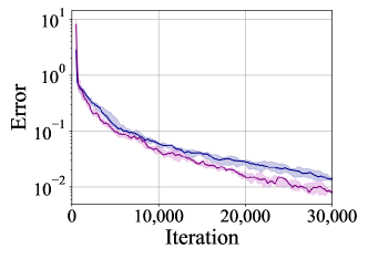
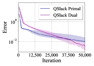
Penalty value

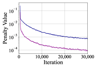
Figure 6: Normalized trace distance error and penalty terms.

H.2 Root fidelity

Figure 7 shows the total error and the penalty value during the optimization as a function of the number of iterations.

	Purification ansatz	Convex-combination ansatz
Error
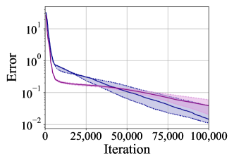
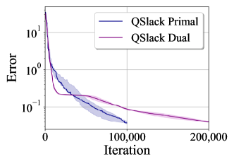
Penalty value

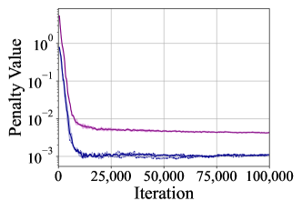
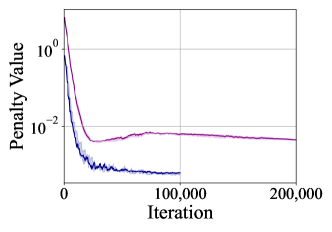
Figure 7: Root fidelity error and penalty terms.

H.3 Entanglement negativity

Figure 8 shows the total error and the penalty value during the optimization as a function of the number of iterations.

	Purification ansatz	Convex-combination ansatz
Error
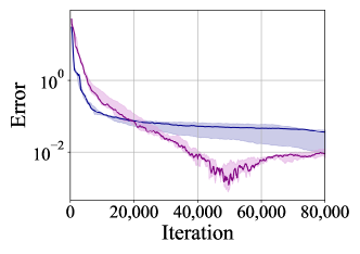
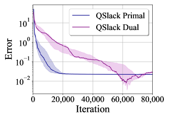
Penalty value

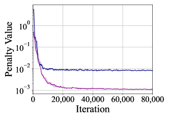
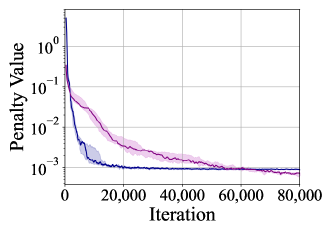
Figure 8: Entanglement negativity error and penalty terms.

H.4 Constrained Hamiltonian optimization

To showcase our algorithm, we considered the following example two-qubit Hamiltonian:

$$H=\sigma_{Z}^{1}\otimes\sigma_{Z}^{2}+\sigma_{X}^{1}\otimes\sigma_{I}^{2}+\sigma_{I}^{1}\otimes\sigma_{X}^{2},$$ (482)

and the following constraints:

$$A_{1} =\sigma_{Y}\otimes\sigma_{I},\qquad b_{1}=0.2,$$ (483)

$$A_{2} =\sigma_{I}\otimes\sigma_{Z},\qquad b_{2}=0.1.$$ (484)

Figure 9 shows the total error and the penalty value during the optimization as a function of the number of iterations.

	Purification ansatz	Convex-combination ansatz
Error
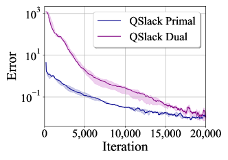
Penalty value

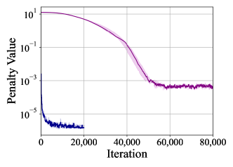
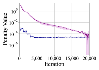
Figure 9: Error and penalty values for the constrained Hamiltonian optimization problem with the true value $-2.2097$.

Problem		Number of Qubits	Number of Layers	Penalty parameter	Learning Rate	Gradient
Total variation distance	Primal	$2$	$2$	$10$	Decreasing rate scheme (300)	Normalized SPSA
	Dual	$2$	$2$	$100$
Constrained classical Hamiltonian	Primal	$2$	$3$	$10$	Decreasing rate scheme (300)	Normalized SPSA
	Dual	$2$	$3$	$10$

Table 3: Details of CSlack simulations.

H.5 Total variation distance

The simulation results for both the primal and dual optimizations of the total variation distance on two probability distributions resulting from two-qubit quantum circuit Born machines are shown in Figure 4. Plots showing decreasing error and penalty values across training are given in Figure 10.

Error	Penalty value

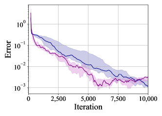
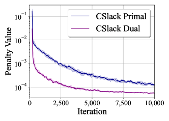
Figure 10: Error and penalty values for the total variation distance problem.

H.6 Constrained classical Hamiltonian optimization

In our simulations, the inputs were selected to be the following Hamiltonian vector, constraint vectors, and constraint values:

$$h =s_{1}\otimes s_{1},$$ (485)

$$a_{1} =0.5(s_{1}\otimes s_{0}),\qquad b_{1}=0.1,$$ (486)

$$a_{2} =0.7(s_{0}\otimes s_{1}),\qquad b_{2}=0.3.$$ (487)

The simulation results for both the primal and dual of this problem instance are shown in Figure 4. Plots showing decreasing error and penalty values across training are given in Figure 11.

Error	Penalty value

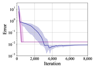
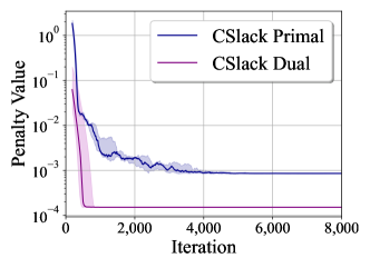
Figure 11: Error and penalty values for the constrained classical Hamiltonian optimization problem.

Appendix I Barren plateau analysis

Given the broad applicability of QSlack and CSlack, a complete discussion of all possible ways in which barren plateaus could manifest or be avoided in this framework would be formidable. As such, we only aim to provide an overview of some of the key considerations here.

Background.

A barren plateau is a cost landscape for which the magnitudes of gradients vanish exponentially with problem size [87]. This phenomenon has been shown to be equivalent to exponential concentration, in which the loss concentrates with high probability to a single fixed value [3]. On such landscapes, training with a polynomial number of measurement shots results in a poorly trained model, regardless of the optimization method employed [2]. More precisely, exponential concentration can be formally defined as follows.

Definition 20 (Exponential concentration)

Consider a quantity $X(\alpha)$ that depends on a set of variables $\alpha$ and can be measured from a quantum computer as the expectation of some observable. $X(\alpha)$ is said to be deterministically exponentially concentrated in the number $n$ of qubits towards a certain fixed value $\mu$ if

$$|X(\alpha)-\mu|\leq\beta\in O(1/b^{n})\;,$$ (488)

for some $b>1$ and all $\alpha$. Analogously, $X(\alpha)$ is probabilistically exponentially concentrated if

$${\rm Pr}_{\alpha}[|X(\alpha)-\mu|\geq\delta]\leq\frac{\beta}{\delta^{2}}\;\;,\;\beta\in O(1/b^{n})\;,$$ (489)

for $b>1$. That is, the probability that $X(\alpha)$ deviates from $\mu$ by a small amount $\delta>0$ is exponentially small for all $\vec{\alpha}$.

The barren-plateau phenomenon has predominantly been studied in the context of losses of the form

$$C(\theta)=\text{Tr}[OU(\theta)\rho U(\theta)^{\dagger}]\;,$$ (490)

where $\rho$ is an $n$-qubit input state and $O$ is a Hermitian operator.

While a complete analysis of the barren plateau phenomenon requires the interplay between the choice of parameterized quantum circuit and measurement operations to be considered in conjunction [105, 45], in the case of problem-agnostic ansätze, a good first step to assessing whether a problem will exhibit a barren plateau is to determine whether it is local or global. It was shown in [35] that, for random hardware efficient ansätze, global costs (i.e., ones for which $O$ acts non-trivially on $\mathcal{O}(n)$ qubits), exhibit barren plateaus at all depths. In contrast local costs, that is losses where the measurement acts non-trivially on at most $\log(n)$ qubits, can exhibit gradients that vanish at worst polynomially (i.e. do not have a barren plateau). For this guarantee to hold, the initial state needs to not be too entangled or too mixed. In particular, the $\log(n)$ marginals of the initial state must not be exponentially close to maximally mixed.

QSlack.

The purification ansatz naturally fits into this framework and it can be shown that the convex combination ansätze (both standard and correlated) can also be understood through this lens with a little thought. We first note that the standard (uncorrelated) convex combination ansatz can be written in the form of (490) by taking the initial state as $\rho=\sum_{x}p_{\varphi}(x)|x\rangle\!\langle x|$. To study the case of the correlated convex combination ansatz, we then note that whether the cost is optimized via gradient descent directly or using a tensor network, ultimately what matters in both cases are cost gradients [2]. Hence we can consider a simplified version of the correlated convex combination ansatz that takes the form

$$\rho(\varphi,\gamma)=\sum_{x}p_{\varphi}(x)U(\gamma_{x})|x\rangle\!\langle x|U(\gamma_{x})^{{\dagger}}\,,$$ (491)

and so the cost under consideration is

$$C(\varphi,\gamma)=\sum_{x}p_{\varphi}(x)\text{Tr}[OU(\gamma_{x})|x\rangle\!\langle x|U(\gamma_{x})^{{\dagger}}]\;.$$ (492)

While this is not of precisely the same form as (490), given that the parameters for each circuit in the convex combination are independent of those in the other terms, the other terms vanish upon differentiation. For example, consider the derivative with respect to the $j$th component of the $\gamma_{x}$ parameter vector. In this case the partial derivative takes the form

$$p_{\varphi_{1}}(x)\partial_{\gamma_{x}^{j}}\text{Tr}\left[U(\gamma_{x})|x\rangle\!\langle x|U(\gamma_{x})^{{\dagger}}O\right]\,,$$ (493)

which is of precisely the same structure as taking the partial derivative of a single component of $\theta$ in (490). Hence the standard barren plateau analysis carries over to the correlated convex combination ansatz.

Whether or not QSlack utilises global or local costs depends on the precise application to which it is applied. For example, for the case of constrained Hamiltonian optimization, as applied to local Hamiltonians (as it typical in many physically motivated cases), QSlack can involve only local costs. In this case the purification ansatz and correlated convex combination ansatz provably avoid barren plateaus for shallow hardware efficient circuits. The case of the standard convex combination ansatz is a little more subtle with the trainability also depending on the initial state. If the initial state from the generative model, i.e. $\rho=\sum_{x}p_{\varphi}(x)|x\rangle\!\langle x|$ is too close to maximally mixed, then even for shallow circuits and local Hamiltonians the landscape can exhibit a barren plateau. Hence careful consideration will need to be taken for the choice in initial distribution for $p_{\varphi}(x)$.

In the case of the examples of trace distance, root fidelity, and entanglement negativity, global terms do appear in the costs, which are likely to lead to trainability difficulties for unstructured ansätze. However, it is worth stressing at this point that barren plateaus are an average phenomenon, and it is possible that these difficulties could potentially be side stepped if one can develop clever initialization strategies. Whether such strategies could be developed in the context of QSlack remains an open question. Furthermore, whether or not they can may well depend on properties of the solution state, with highly mixed and highly random targets likely to prove more challenging to learn [57].

CSlack.

When a quantum circuit Born machine is used with CSlack one also needs to consider trainability concerns. The overlap terms $\sum_{x}p(x)t(x)$, as measured using the collision test, correspond to ‘explicit’ costs and hence are subject to barren plateaus [109]. To see this note that in the collision test one is computing the expectation value of a Kronecker delta function, i.e., $\sum_{x}p(x)t(x)=\langle\delta_{x,y}\rangle_{x\sim p,y\sim t}$. The core problem is that one only obtains a signal in the collision test in the case that one draws two identical bit strings. However, if the distributions have exponential support, the probability of this occurring is exponentially small in general. Hence, with finite shots, the overlap will be precisely zero for nearly all parameter settings, making meaningful training practically impossible.

One way one could attempt to resolve this would be to replace the Kronecker delta with a Gaussian kernel, as is done in the Maximum Mean Discrepancy loss used in generative modeling. That is, one could use the fact that $\sum_{x}p(x)t(x)=\lim_{\sigma\rightarrow 0}\langle e^{-|x-y|/\sigma^{2}}\rangle_{x\sim p,y\sim t}$, train initially with a finite $\sigma$ value (for which a larger signal should be observed), and then slowly decrease the $\sigma$ value during training to regain the original cost value. While we believe this suggestion is original in this context, a similar approach has been discussed in the context of generative modeling and would be a good reference to understand this suggestion further [109].