Dynamics of spin-momentum entanglement from superradiant phase transitions

Abstract

Exploring operational regimes of many-body cavity QED with multi-level atoms remains an exciting research frontier for their enhanced storage capabilities of intra-level quantum correlations. In this work, we propose an extension of a prototypical many-body cavity QED experiment from a two to a four-level description by optically addressing a combination of momentum and spin states of the ultracold atoms in the cavity. The resulting model comprises a pair of Dicke Hamiltonians constructed from pseudo-spin operators, effectively capturing two intertwined superradiant phase transitions. The phase diagram reveals regions featuring weak and strong entangled states of spin and momentum atomic degrees of freedom. These states exhibit different dynamical responses, ranging from slow to fast relaxation, with the added option of persistent entanglement temporal oscillations. We discuss the role of cavity losses in steering the system dynamics into such entangled states and propose a readout scheme that leverages different light polarizations within the cavity. Our work paves the way to connect the rich variety of non-equilibrium phase transitions that occur in many-body cavity QED to the buildup of quantum correlations in systems with multi-level atom descriptions.

I Introduction

The coupling between spin and motional degrees of freedom lies at the root of several rich phenomena in quantum physics, including fine structure splitting of atoms Sakurai and Commins (1995) and the spin Hall effect Hirsch (1999), which, in turn, allow the realization of topological phases of matter Hasan and Kane (2010); Sato and Ando (2017) and open the possibility of topological quantum computing Sau et al. (2010); Qi et al. (2023a). Spin-momentum entanglement resulting from such coupling has increasingly become relevant in a variety of research areas, ranging from materials science to photonics and atomic systems Stav et al. (2018); Kale et al. (2020); Manzoni et al. (2017). In this work, we propose a protocol for engineering entanglement between the spin and momentum degrees of freedom of ultracold atoms coupled to an optical cavity. Our approach exploits a non-equilibrium superradiant phase transition in the system realized by coupling four atomic modes, which comprise two internal (spin) and external (momentum) states of the atom.

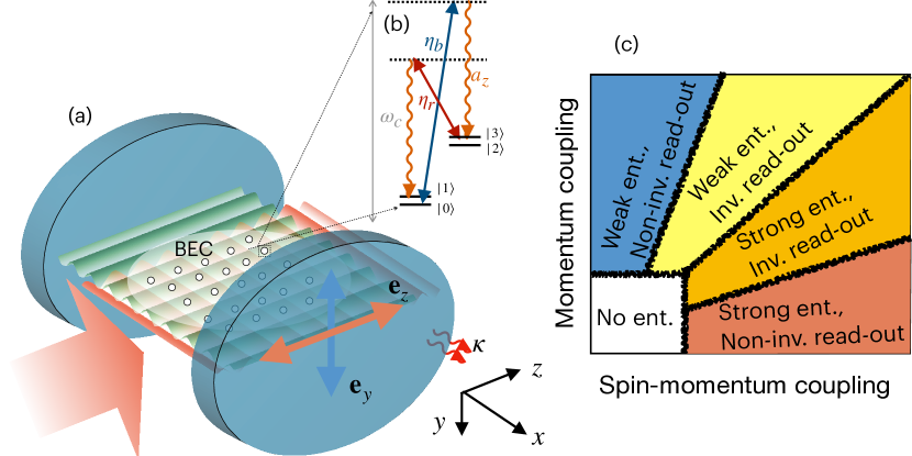
Figure 1: (a) Sketch of the cavity QED setup and (b) of the atomic level scheme. (c) Cartoon of the dynamical phase diagram as a function of the couplings between spin and momentum degrees of freedom.

Many-body cavity QED experiments with ultracold atoms are among the most versatile quantum simulators of driven-dissipative phases of matter Mivehvar et al. (2021). The combination of tunable photon-mediated long-range interatomic interactions, along with strong cooperative effects and control on cavity losses, offers a wide range of possibilities, encompassing non-equilibrium transitions Dogra et al. (2019); Baumann et al. (2010); Kroeze et al. (2019); Marino et al. (2022); Klinder et al. (2015); Skulte et al. (2021); Kongkhambut et al. (2021, 2022); Lewis-Swan et al. (2021); Carollo and Lesanovsky (2021), dynamical control of correlations Seetharam et al. (2022a, b); Marino (2022); Periwal et al. (2021); Finger et al. (2023); Rosa-Medina et al. (2022), realization of dark states Lin et al. (2022); Skulte et al. (2023); Piñeiro Orioli et al. (2022), and the exploration of collective phenomena purely driven by engineered dissipation  Soriente et al. (2018); Landini et al. (2018); Dreon et al. (2022). Oftentimes, the effective atomic degrees of freedom in state-of-art experiments are a pair of momentum states or internal levels, optically addressed by external laser drives inducing cavity-assisted two-photon transitions Nagy et al. (2010); Baumann et al. (2010); Zhiqiang et al. (2017); Masson et al. (2017). Recently, a few cavity QED experiments and theory works have shown how to couple the momentum and internal spin degrees of freedom of ultracold atoms using intra-cavity light, demonstrating novel self-organized phases  Ferri et al. (2021); Kroeze et al. (2018); Dogra et al. (2019); Mivehvar et al. (2017); Wilson et al. (2022).

In this paper, we generalize such protocols to show that spin-momentum entanglement can be synthesized, controlled, and steered in experiments by coupling motional and internal degrees of freedom. We consider a cavity QED platform, cf. Fig. 1(a), which is described by a minimal model with two different spin states and two different momentum states, meaning that each atom can occupy one of these four hybrid spin-momentum states shown in Fig. 1(b). We demonstrate that this system exhibits superradiant phase transitions related to the self-organization of the atoms in the cavity, concomitantly with the dynamical buildup of spin-momentum entanglement. By varying the spin-momentum coupling, one can robustly tune the entanglement up to its maximum possible value.

The superradiant phase transitions within this model exhibit notable distinctions from the conventional phenomenology of self-organization in cavity QED  Dogra et al. (2019); Baumann et al. (2010); Nagy et al. (2010, 2011); Stitely et al. (2022); Lerose and Pappalardi (2020); Defenu et al. (2023); Kirton et al. (2019); Landini et al. (2018); Dreon et al. (2022). While the hybrid spin-momentum order parameter in our system and the photon number approach stationary values, the spin and momentum separately can be non-stationary. This results in a time-dependent profile of the condensate density and the effective spin magnetization, which is unconventional for state-of-art cavity QED experiments Ferri et al. (2021); Kroeze et al. (2018). Such oscillations persist beyond the operational time scales of these platforms, resulting in long-lived non-stationary dynamical responses. We show that such features can be continuously probed using an auxiliary cavity field, which is coupled to the momentum degree of freedom of atoms. The overall dynamics in such a model are conditioned by the intertwining of two cavity-mediated processes, controlled by two couplings between momentum states or hybrid momentum-spin states. The different dynamical responses of the system, summarized in Fig. 1(c), are characterized by weak or strong entanglement. In particular, despite the back-action and intrinsic decoherence of the read-out process, proxy of spin-momentum entanglement dynamics can be non-invasively accessed in an extended parameter regime [red region in Fig. 1(c)], making the system a possible candidate for quantum information applications Nielsen and Chuang (2010).

Crucially, in our scheme, cavity losses have the beneficial role of steering dynamics towards target entangled states, thereby endowing robustness to the initial condition of the system. This feature is absent in protocols engineering spin-momentum entanglement in BECs using solely classical drive fields Kale et al. (2020). In such proposals, the degree of achievable spin-momentum entanglement is highly sensitive with respect to technical fluctuations of different experimental parameters (e.g., drive powers and frequencies). In contrast, protocols relying on cavity losses induce contractive dynamics which are insensitive to such issues and initial state preparation, therefore offering a more robust and reliable route for spin-momentum entanglement generation.

I.1 Outline of the article

The paper is organized as follows. In Sec. II, we present an experimentally motivated effective model that governs the dynamics of the cavity QED setup in Fig. 1, where the spin and momentum of atoms are coupled to the cavity field. Sec. III is devoted to the superradiant phase transition and subsequent generation of entanglement between spin and momentum degrees of freedom. In Sec. IV, we extend the model by introducing an auxiliary cavity mode and show how it enables continuous read-out of the system dynamics. In Sec. V, we analyze the dynamical responses and read-out strategies. In Sec. VI, we revisit entanglement generation in the presence of the auxiliary cavity mode and discuss prospects for its non-invasive read-out. In the concluding Section VII, we summarize our findings and discuss follow-up directions.

II Model

We consider a cavity QED configuration in which we can address both the spin and momentum states of ultracold atoms, enabling measurement and dynamic control (see also Ref. Ferri et al. (2021) for a related setup). Specifically, we consider Bose-Einstein condensate (BEC) of ⁸⁷Rb atoms in the $F=1$ hyperfine ground state manifold confined in a high-finesse optical cavity. The atoms are coupled to a $z$-polarized cavity mode $a_{z}$ with resonance frequency $\omega_{c}$ and decay rate $\kappa$, extending along $x$ direction, as illustrated in Fig. 2(a). A bias magnetic field $\vec{B}$ along the ${z}$ direction defines the quantization axis and induces Zeeman splitting between the sub-levels of the $F=1$ hyperfine manifold. We focus on two internal atomic sub-levels $\ket{m_{F}=1}=\ket{\downarrow}_{s}$ and $\ket{m_{F}=0}=\ket{\uparrow}_{s}$, and describe the condensate with the spinor wave function $\Psi=\left(\psi_{\uparrow},\psi_{\downarrow}\right)^{T}$.

The condensate is illuminated with transverse standing-wave laser fields far-detuned from the electronic transitions of the atoms. These detunings allow us to effectively eliminate the contribution of excited electronic states and to focus on the near-resonant cavity-assisted two-photon transitions between momentum atomic states $\ket{0}_{m}=\ket{k_{x}=0,k_{z}=0}$ and $\ket{1}_{m}=\ket{k_{x}=\pm k,k_{z}=\pm k}$. Here, $\hbar k=2\pi\hbar/\lambda$ indicates the recoil momentum, with $\lambda/2=784.7/2\mathrm{~{}nm}$ representing the period of the standing wave potential along the drive direction.

We introduce the following definitions of relevant combinations of momentum and spin states [cf. Fig. 2(b)]

$$\ket{0} =\ket{0}_{m}\otimes\ket{\downarrow}_{s},$$ (1)

$$\ket{1} =\ket{1}_{m}\otimes\ket{\downarrow}_{s},$$

$$\ket{2} =\ket{0}_{m}\otimes\ket{\uparrow}_{s},$$

$$\ket{3} =\ket{1}_{m}\otimes\ket{\uparrow}_{s},$$

limiting our consideration to a four-level model of the system, which will be further justified in the following. In this notation, even states $\ket{0}\textrm{ and }\ket{2}$ are momentum ground states that correspond to the homogeneous condensate density in real space, while odd states $\ket{1}\textrm{ and }\ket{3}$ are excited momentum states and correspond to a modulation of the atomic density in real space: $\ket{1}_{m}\propto\cos kx\cos kz$ (see also Ref. Baumann et al. (2010)). We also introduce boson annihilation and creation operators $c_{0,\ldots,3},~{}c_{0,\ldots,3}^{\dagger},$ $[c_{i},c_{j}^{\dagger}]=\delta_{i,j},$ which describe the annihilation and creation of a particle in these four state manifold of Eqs. (1).

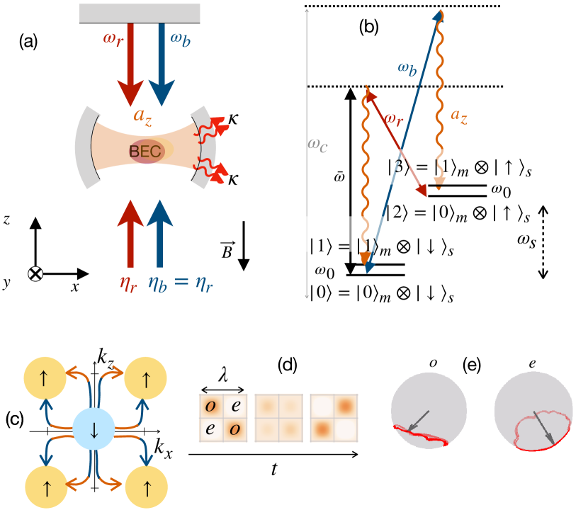
Figure 2: (a) Schematics of the experimental setup and (b) corresponding level scheme for the model (2). (c) Momentum space cartoon for spin-flipping Raman process for a transition $\ket{0}\to\ket{3}$; (d) Snapshots of the real-space BEC density in the $\ket{\uparrow}_{s}$ manifold at different times; (e) Dynamics in the superradiant phase of the spin components on even ($e$) and odd ($o$) lattice sites plotted on the Bloch spheres.

We consider Raman processes that simultaneously couple internal (spin) and external (momentum) atomic degrees of freedom Ferri et al. (2021); Kroeze et al. (2018); Zhang et al. (2018). These processes are mediated by the interaction of the cavity mode $a_{z}$ and two classical driving fields with coupling strength $\eta_{b}=\eta_{r}=\eta$ and frequencies $\omega_{b},$ $\omega_{r},$ with $2\bar{\omega}=\omega_{b}+\omega_{r}$, $\delta=\omega_{b}-\omega_{r}$. In this context, the laser at frequency $\omega_{b}$ facilitates the transition between states $\ket{0}$ and $\ket{3}$, from the ground momentum state $|0\rangle_{m}$ to the excited momentum state $|1\rangle_{m}$, accompanied by a spin flip from $|\downarrow\rangle_{s}$ to $|\uparrow\rangle_{s}$ and vise versa. Conversely, the laser at frequency $\omega_{r}$ induces a similar transition, $\ket{2}\leftrightarrow\ket{1}$, accompanied by a spin flip from $|\uparrow\rangle_{s}$ to $|\downarrow\rangle_{s}$, cf. Fig. 2(b,c). These two cavity-assisted Raman processes mediate an interaction of the form $\eta\left(a_{z}+a_{z}^{\dagger}\right)\cos kx\cos kz(F^{+}+F^{-}),$ where the spin operators $F^{\pm}$ couple simultaneously ground and excited momentum states on the neighboring spin levels [cf. momentum cartoon in Fig. 2(c) and Appendix A for the model details]. After integrating over the spatial extent of the condensate, the Hamiltonian of the effective model reads

$$H =\omega_{z}a_{z}^{\dagger}a_{z}+(\omega_{0}-\omega_{s})S_{12}^{z}+(\omega_{0}+\omega_{s})S_{03}^{z}$$ (2)

$$+2\eta\left(a_{z}+a_{z}^{\dagger}\right)\left(S_{12}^{x}+S_{03}^{x}\right),$$

where $\omega_{z}$ is the cavity detuning, $\omega_{0}$ is the double recoil energy $\omega_{\operatorname{rec}}=k^{2}/(2M),$ which atoms acquire in the two-photon process, and $\omega_{s}$ is the effective splitting between the two spin manifolds. We set $\hbar=1$ to keep the notation compact.

The cavity boson field $a_{z}$ satisfies the commutation relations $[a_{z},a_{z}]=0,$ $[a_{z},a_{z}^{\dagger}]=1.$ The collective pseudo-spin operators $S$ are built as projectors between the macroscopically occupied spin-momentum levels $S_{ij}^{-}=\ket{i}\bra{j}=c_{i}^{\dagger}c_{j}$, $S_{ij}^{+}=(S_{ij}^{-})^{\dagger},$ $S_{ij}^{z}=(c_{j}^{\dagger}c_{j}-c_{i}^{\dagger}c_{i})/2,$ $S_{ij}^{x}=(S_{ij}^{-}+S_{ij}^{+})/2$ for $i=0,\ldots,3<j.$ Here, we already rescaled spin and photon operators via $S\to S/N,$ $a_{z}\to a_{z}/\sqrt{N}$ (and also $c_{i}\to c_{i}/\sqrt{N}$) as it is convenient for collective spin models Kirton et al. (2019); Chelpanova et al. (2023), where $N$ is a number of atoms in the condensate.

The dynamics of the system are described by the Lindblad master equation for the density matrix $\rho$

$$\frac{d}{dt}\rho=-i[H,\rho]+\kappa\mathcal{D}(\rho)$$ (3)

$$\mathcal{D}(\rho)=2a_{z}\rho a_{z}^{\dagger}-\left\{a_{z}^{\dagger}a_{z},\rho\right\}.$$

where cavity losses account for the finite lifetime of the cavity photon $a_{z}.$

Our proposal is inspired by the experiments reported in Refs. Ferri et al. (2021); Dogra et al. (2019) that typically involve a substantial number of atoms, around $N\approx 10^{4}-10^{5}$, and deviations from mean-field behavior only become pronounced at extremely long timescales. The coupling between photons and atoms is collective [cf. Eq. (2)], and results in a suppression of light-matter correlations by a factor of $1/N$. The dynamics are thus well captured by mean-field equations of motion, which we report in Appendix B for completeness. However, correlations between the spin and momentum degrees of freedom within the condensate play a significant role in entanglement dynamics, as we show in detail in the following Section.

The dynamics in Eq. (3) possess a $\mathbb{Z}_{2}$ symmetry characteristic of Dicke models Dicke (1954); Dimer et al. (2007); Ferri et al. (2021); Kroeze et al. (2018); Nagy et al. (2010): it is invariant under the transformation $(a_{z},S^{x})\leftrightarrow(-a_{z},-S^{x}),$ where $S^{x}=S_{03}^{x}+S_{12}^{x}$ [cf. Eq. (2)]. When this symmetry is spontaneously broken, the system undergoes a phase transition. In the thermodynamic limit, the transition can shift the system from the trivial normal state with the empty cavity mode $n_{z}=\langle a_{z}^{\dagger}a_{z}\rangle=|\langle a_{z}\rangle|^{2}=0$ and all spins polarized along the $z$ direction to the superradiant (SR) phase with the non-zero occupation of the cavity mode and finite ${x}$ component of the spin, namely $n_{z}\neq 0$ and $\langle S^{x}\rangle\neq 0$ (cf. Appendix D or Ref. Kirton et al. (2019) for more details). Throughout this paper, we employ $\langle\cdot\rangle$ to denote expectation values of observables.

When $\omega_{s}=0$, the critical coupling at which the transition to the SR phase takes place read $\eta_{\omega_{s}=0}^{c}=[\omega_{0}(\omega_{z}^{2}+\kappa^{2})/(4\omega_{z})]^{1/2}$ Dicke (1954); Kirton and Keeling (2018), while for $\omega_{s}\neq 0$ case, the critical coupling becomes sensitive to the initial conditions. This sensitivity is rooted in the different effective level splitting for pseudo-spins $S_{03}$ and $S_{12}$, $\omega_{0}\pm\omega_{s}$. The specific distribution of particles between the two pseudo-spins, $S_{03}$ and $S_{12}$, gives rise to distinct effective level splittings between excited and ground momentum states, and thus different critical couplings. A similar dependence on the initial state also emerges when there is disorder in the coupling constants, as discussed in Refs. Mivehvar (2023); Marsh et al. (2023).

To illustrate this dependence, consider initialization of the system in a mixture of the atoms in the ground momentum state, $|k_{x},k_{z}\rangle=|0\rangle_{m}$, with two different magnetic numbers; namely, we prepare $N_{0}=N\langle c_{0}^{\dagger}c_{0}\rangle=\mu N$ particles in level $|0\rangle$ and $N_{2}=N\langle c_{2}^{\dagger}c_{2}\rangle=(1-\mu)N$ particles in level $|2\rangle$, where $\mu\in[0,1]$. This results in the critical coupling (see Appendix D)

$$2\eta^{c}=\begin{cases}\sqrt{\frac{\left(\omega_{0}^{2}-\omega_{s}^{2}\right)\left(\omega_{z}^{2}+\kappa^{2}\right)/\omega_{z}}{\left(\omega_{s}+\omega_{0}\right)-2\mu\omega_{s}}},&\omega_{s}<\omega_{0}\\ \sqrt{\frac{\left(\omega_{s}^{2}-\omega_{0}^{2}\right)\left(\omega_{z}^{2}+\kappa^{2}\right)/\omega_{z}}{\left(\omega_{s}+\omega_{0}\right)-2\mu\omega_{0}}},&\omega_{s}>\omega_{0}.\end{cases}$$ (4)

For $\eta>\eta_{c}$, the cavity mode occupation $n_{z}=\langle a_{z}^{\dagger}a_{z}\rangle$ and the $\langle S^{x}\rangle$ pseudo-spin components take non-zero values in the steady state. In terms of atomic degrees of freedom, the SR transition is characterized by the emergence of spatial ordering with a periodicity $\lambda=2\pi/k$, see Refs. Baumann et al. (2010); Kroeze et al. (2018); Ferri et al. (2021); Dogra et al. (2019); Klinder et al. (2015). This spatial ordering can be associated with the modulation of the condensate density or spin orientation along the lattice. More precisely, the density of the condensate in the upper (lower) spinor components read $|\psi_{\downarrow}|^{2}\approx|\langle c_{0}\rangle+\langle c_{1}\rangle\cos kx\cos kz|^{2}$ ($|\psi_{\uparrow}|^{2}\approx|\langle c_{2}\rangle+\langle c_{3}\rangle\cos kx\cos kz|^{2}$), and, depending on the ratio between $\langle c_{0}\rangle$ and $\langle c_{1}\rangle$ ($\langle c_{2}\rangle$ and $\langle c_{3}\rangle$), its periodicity can vary between $\lambda$ when $\mu\neq 0,1$ [left and right panels in Fig. 2(d)] and $\lambda/2$ when $\mu=0,1$ [middle panel in Fig. 2(d)]. This ratio is set by the initial conditions and $\eta/\eta^{c}$. When the periodicity of the real-space condensate density deviates from $\lambda$, the correct spatial ordering can be established by the spin checkerboard lattice. This involves a distinction in the polarization of spins on even and odd lattice sites Kroeze et al. (2018). As we illustrate below, in the most general case, there is a periodical exchange between density- and spin-modulated lattices to form correct spatial ordering with the periodicity $\lambda$.

Going beyond effective two-level models in Refs. Ferri et al. (2021); Kroeze et al. (2018), the four-level model we consider in this work features the possibility of non-stationary spin-momentum configurations in the SR phase. These non-stationary solutions emerge from the intrinsic nature of the pseudo-spin $S$, which is neither purely momentum nor purely an internal degree of freedom. Consequently, the mere presence of a non-zero stationary value of $\left\langle S^{x}\right\rangle$ in the SR phase does not guarantee stationary expectation values for the spin or momentum degrees of freedom. In particular, in the SR phase, atomic spin precession occurs at frequency $\Omega\propto 2\omega_{s}$ with an amplitude $\propto\sqrt{\mu(1-\mu)}$. This leads to periodic density modulations alternating between even and odd lattice sites, as shown in Fig. 2(d,e).

For the experiments in Refs. Ferri et al. (2021); Dogra et al. (2019), the key parameters are $\omega_{0}/(2\pi)\approx 7.4\mathrm{kHz}$ and $\kappa/(2\pi)=1.25\mathrm{MHz}$. The remaining detunings and coupling strengths are tunable, allowing for the exploration of a broad spectrum of dynamical regimes. In the next Sections, we study the entanglement between spin and momentum during such dynamics and then show how such non-stationary phases can be probed in the experiment.

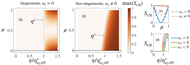
Figure 3: (a-b) Maximum of spin-momentum entanglement $S_{\operatorname{vN}}$ as a function of $\eta/\eta_{\omega_{s}=0}^{c}$ and $\mu$. Entanglement is built up as we enter the superradiant phase. Here (a) $\omega_{s}=0$ and (b) $\omega_{s}=\omega_{0}/4$. (c) Maximal (solid lines) and time-averaged (dashed lines) entanglement entropy as a function of $\mu$ for different values of $\omega_{s}$ and $\eta/\eta_{\omega_{s}=0}^{c}=1.5.$ (d) Maximal (solid lines) and time-averaged (dashed lines) entanglement entropy as a function of photon-matter coupling $\eta$ for $\mu=0$. Different colors indicate different $\omega_{s}$.

III Spin-momentum entanglement and superradiant dynamics

Although correlations among different atoms are negligible, our platform offers a route to engineer robust entanglement between spin and momentum degrees of freedom within the bosonic condensate trapped in the cavity. For instance, assume all atoms are initially prepared in the state $|0\rangle=|0\rangle_{m}\otimes|\downarrow\rangle_{s}$. Through the interaction with the cavity mode $a_{z}$, the atoms are coupled to the state $|3\rangle=|1\rangle_{m}\otimes|\uparrow\rangle_{s}$ as $2\eta(a_{z}+a_{z}^{\dagger})S_{03}^{x}\ket{0}=\eta(a_{z}+a_{z}^{\dagger})\ket{3}$. Thus, in the SR phase with the non-zero cavity field ($\langle a_{z}\rangle\neq 0$), the cavity-mediated interaction gives rise to a non-separable spin-momentum state. The corresponding state of each atom reads

$$\ket{\psi}=\langle c_{0}\rangle|0\rangle_{m}\otimes|\downarrow\rangle_{s}+\langle c_{3}\rangle|1\rangle_{m}\otimes|\uparrow\rangle_{s},$$ (5)

with $\langle c_{0}\rangle\neq 0$ and $\langle c_{3}\rangle\neq 0,$ and $|\psi\rangle$ is a non-separable entangled state of spin and momentum. Our results will revolve around the dynamical manipulation of this form of entanglement.

In order to quantify spin-momentum entanglement, we use the von Neumann entropy

$$S_{\operatorname{vN}}=-\Tr\left({\tilde{\rho}}\log_{2}{\tilde{\rho}}\right)$$ (6)

with $\tilde{\rho}$ the reduced density matrix after tracing out spin or momentum states, cf. Appendix E. When the system is in a product state of spin and momentum, the entanglement vanishes and $S_{\operatorname{vN}}=0$. With the definition in Eq. (6), a maximally entangled state has $S_{\operatorname{vN}}=1.$ We also compute negativity Cornfeld et al. (2018) and concurrence Wootters (2001); Zou et al. (2022), which are more reliable witnesses of entanglement in open systems Vidal and Werner (2002). However, they show the same qualitative behavior as $S_{\operatorname{vN}}$ (cf. Appendix E), and thus we restrict our analysis to the von Neumann entropy for its simplicity.

By adjusting coupling $\eta$ and the initial state of atoms, we compute a dynamical phase diagram, which captures maximal $S_{\operatorname{vN}}$ reached during evolution, see Fig. 3. The system is initially prepared in the normal state with $N_{0}=\mu N$ atoms in the state $\ket{0}$, after which we rapidly increase the coupling $\eta$ to a specified value. The equations of motion describing this process can be found in Appendices B and C. Note that the collective description of the model, adapted in this work, is valid only when the system is prepared in the permutation invariant state; otherwise, dynamics become more complicated as discussed in Huybrechts et al. (2020); Qi et al. (2023b); Iemini et al. (2023); Valencia-Tortora et al. (2023). Below, we analyze the entanglement properties for both the degenerate case $\left(\omega_{s}=0\right)$ and the non-degenerate case $\left(\omega_{s}\neq 0\right)$, showcasing the potential for achieving either a stationary or a time oscillating amount of entanglement, respectively.

III.0.1 Degenerate $\omega_{s}=0$ case

The amount of $S_{\operatorname{vN}}$ reached during dynamics in the degenerate case is shown in Fig. 3(a). Depending on the initial configuration, the maximum amount of entanglement in the system can vary from $\max(S_{\operatorname{vN}})=0$ to $\max(S_{\operatorname{vN}})=1.$ Specifically, when $\mu=0.5,$ the momentum configuration of each spin component reads exactly the same, and the state becomes separable. Conversely, when $\mu=0$ or $1,$ one can reach a maximally entangled state; the dependence of the entanglement in the system as a function of $\mu$ is shown with blue lines in Fig. 3(c). On the other hand, the amount of entanglement in the SR phase depends on the coupling $\eta$, [cf. dependence of the entanglement entropy as a function of coupling for $\mu=0$ in panel (d), blue lines]. Here, entanglement increases with the coupling which can be qualitatively understood as follows. When $\eta\approx\eta^{c},$ almost all atoms occupy the ground momentum state and $\ket{\psi}\propto\ket{2}$, which is separable in terms of spin and momentum. However, as we increase coupling, the population of the excited momentum level $\ket{1}$ increases and the spin-momentum state of the system becomes non-separable, approaching a maximally entangled state deep in the SR phase.

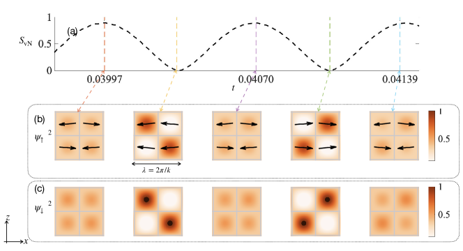
Figure 4: (a) Dynamics of entanglement, (b) density of the upper spinor component with corresponding spin orientation, and (c) density of the lower spinor component. Entropy is maximized when the state $\ket{\psi}$ is a non-separable combination of two spin-momentum states, and SR manifests as a spin checkerboard lattice. When entanglement vanishes, both spinor components have the same density profile and spin magnetization. Dynamics are simulated for $\mu=0.5,$ $\eta=1.6\eta^{c},$ $\omega_{s}=\omega_{0}/4,$ $\omega_{z}=\kappa.$

III.0.2 Non-degenerate $\omega_{s}\neq 0$ case

When $\omega_{s}\neq 0,$ the dynamical behavior of the entanglement entropy changes compared to the degenerate case [see Fig. 3(b)]. First, the critical coupling depends on $\mu$, cf. Eq. (4). Second, when $\mu=0.5,$ entanglement decreases but does not disappear completely [red lines in panel (c)]. Here, one can notice the difference between the maximal value of the entanglement (dashed line) and the period-averaged value (solid line), indicating an oscillatory behavior in time. The exceptional case is $\mu=0,1$ where the system evolves towards a stationary SR state. From the standpoint of spin-momentum correlations, this state has maximum (non-oscillatory) entanglement when compared with occurrences at other values of $\mu$.

Fig. 4 depicts the dynamics of the entanglement entropy in the non-degenerate case after the quench during the period (a), along with the (b-c) spin (arrows) and density configurations of atoms. Here, maximally entangled configurations correspond to the case when the checkerboard lattice is formed by the spin degree of freedom (arrows), while the condensate density is periodically modulated with the period $\lambda/2.$ On the contrary, in the configuration with minimal entanglement, all spins are aligned in the same direction (left or right), and the condensate density modulation occurs with a period $\lambda.$

Importantly, the precession of the spin and momentum order parameters in the SR phase results in a cyclic pattern of $S_{\operatorname{vN}}$ over time, devoid of any indications of relaxation or decay [see Appendices B and D for more details]. At different times, the spin and momentum states have different overlaps, resulting in oscillations of the entanglement entropy. This is one of the striking features of our quench protocol: we can steer entanglement dynamics toward an oscillatory regime that persists up to the operational timescales of the experiment.

Notice that entanglement is generated during dynamics starting from product spin-momentum states, and thus, the cavity photon has an active role in building spin-momentum correlations via light-induced interactions. The non-zero cavity field $\langle a_{z}\rangle$ in the SR phase mediates an effective interaction among atoms, which is responsible for entangling them in a non-separable spin-momentum state. At the same time, the role of cavity losses is essential. They steer dynamics towards the fixed point of the Lindbladian, with the remarkable consequence that all entanglement properties derived in the presence of photon losses are robust if compared with what would be achieved with a coherent drive Galitski and Spielman (2013); Lorenzo et al. (2017); Kale et al. (2020). For instance, by replacing the cavity field with a time-dependent drive in $H$ [Eq. (2)], one could also entangle spin and momentum degrees of freedom of the condensate’s atoms. However, the amount of final entanglement produced would depend on details of the driving protocol, such as its duration, frequency decomposition, and other specifics. More importantly, such entanglement would be highly sensitive to noise and imperfections in the drive realization. In contrast, cavity losses induce relaxation of atomic entanglement towards a steady state that remains resilient even for moderate imperfections in the initial state preparation or in the parameters set to drive dynamics into superradiance. In other words, there exists a broad basin of attraction towards prescribed values of entanglement given the system’s initial conditions parameters.

IV Two cavity fields setup
and probes of momentum states

In the previous section, we have shown that cavity dissipation can be utilized to prepare the system in a steady state with desired entanglement properties. In the following sections, we show how, by using the auxiliary polarization mode $a_{y}$ of the cavity field, one can get access to the collective momentum state of the system in a non-destructive fashion.

Inspired by the experimental demonstrations in Refs. Baumann et al. (2010); Dogra et al. (2019) we consider a driving scheme that enables effective coupling of ground and excited atomic momentum states. We consider a cavity-assisted Bragg process involving the transverse driving field with amplitude $\eta_{s}$ and frequency $\bar{\omega}$ and the cavity mode $a_{y}$ with detuning $\omega_{y},$ decay rate $\kappa$, and linear polarization along $y$ [see Fig. 5(a,b)]. This process is reflected in the atom-cavity interaction term, $\propto\eta_{s}(a_{y}+a_{y}^{\dagger})\cos kx\cos kz$ (cf. Appendix A). In this two-photon process, atoms initialized in the ground momentum state $\ket{0}_{m}$ can be excited to the momentum state $\ket{1}_{m}$, while the internal spin state ($\ket{\downarrow}_{s}$ or $\ket{\uparrow}_{s}$) remains unchanged [cf. Fig. 5(c)]. The schematics of this process are encoded in the Dicke Hamiltonian (see Appendix A)

$$H_{s}=\omega_{y}a_{y}^{\dagger}a_{y}+\omega_{0}\left(J_{01}^{z}+J_{23}^{z}\right)+2\eta_{s}\left(a_{y}+a_{y}^{\dagger}\right)\left(J_{01}^{x}+J_{23}^{x}\right).$$ (7)

The collective pseudo-spin operator $J$ is constructed from the different macroscopically occupied spin-momentum states as follows $J_{ij}^{-}=\ket{i}\bra{j}=c_{i}^{\dagger}c_{j},$ $J_{ij}^{+}=(J_{ij}^{-})^{\dagger},$ $J_{ij}^{x}=(J_{ij}^{-}+J_{ij}^{+})/2,$ $J_{ij}^{z}=(c_{j}^{\dagger}c_{j}-c_{i}^{\dagger}c_{i})/2$ and $i=0,\ldots,3<j.$

Depending on the coupling $\eta_{s},$ the system undergoes a phase transition associated with the spontaneous breaking of the $\mathbb{Z}_{2}$ symmetry of the Hamiltonian $H_{s}$, such that the Hamiltonian is invariant under the transformation $(a_{y},J^{x})\leftrightarrow(-a_{y},-J^{x})$. When the coupling is below the critical value $\eta_{s}<\eta_{s}^{c}={[\left(\omega_{y}^{2}+\kappa^{2}\right)\omega_{0}^{2}/\left(4\omega_{y}\right)]^{1/2}}$, the system is in the normal phase where only ground momentum states are occupied, and, respectively, $\langle J_{01}^{z}\rangle+\langle J_{23}^{z}\rangle=-1/2,$ $\langle J_{01}^{x}\rangle=\langle J_{23}^{x}\rangle=0,$ and the cavity is empty, $n_{y}=\langle a_{y}^{\dagger}a_{y}\rangle=|\langle a_{y}\rangle|^{2}=0$ (see Appendix D for more details). In this phase, the condensate is homogeneously distributed within the trap without a checkerboard-like density modulation. When $\eta_{s}>\eta_{s}^{c}$, the system enters a $\mathbb{Z}_{2}$ symmetry-broken superradiant phase with $\langle J^{x}\rangle\neq 0$ and $n_{y}\neq 0$. On a microscopic level, in the SR phase, the standing wave driving field and the cavity field form an interference lattice potential $V\propto\cos kx\cos kz$, and the condensate density is modulated, forming the checkerboard lattice with the period $\lambda=2\pi/k,$ see Fig. 5(d). The density modulation originates from the condensate wave function in each spinor component; in the SR phase, each component has a real space profile $\psi_{\uparrow,\downarrow}\approx\langle c_{0,2}\rangle+\langle c_{1,3}\rangle\cos kx\cos kz.$ At the same time, as it is shown in Fig. 5(e), the internal spin $\langle\mathcal{T}\rangle$ also precesses according to the model (7) with the amplitude $\propto\sqrt{\mu(1-\mu)}$ and frequency $\propto 2\omega_{s}$ (see Appendix D).

The interaction term in Eq. (7) couples different atomic momentum states within the same spin manifold and does not generate entanglement between spin and momentum. Precisely, in the SR phase, the momentum configuration reads exactly the same for each spin manifold $\ket{\uparrow}_{s}$ and $\ket{\downarrow}_{s}$, and the state is separable. However, as we show below, competition between $H$ and $H_{s}$ results in a rich manifold of dynamical responses, which can be probed in a non-destructive way by analyzing the light that leaks out of the cavity Brennecke et al. (2013). As we report further in the text, by tuning $\eta$ and $\eta_{s}$, it is possible to monitor the spin-momentum entanglement generated by $\eta$ in a non-invasive manner. This means that such monitoring can be achieved without substantially altering the underlying dynamics of entanglement.

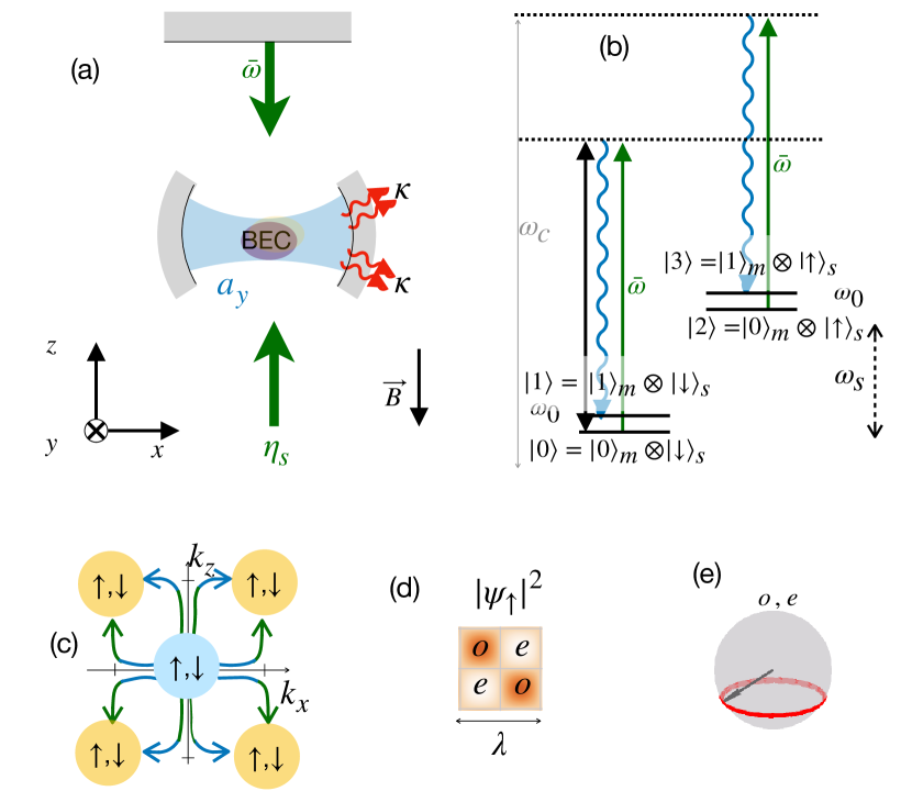
Figure 5: (a) Schematics of the experimental setup and (b) corresponding level scheme for the model (7). (c) Momentum space cartoon for the spin-preserving Bragg process; (d) steady-state density of the condensate in the SR phase; (e) internal spin precession described by the Hamiltonian $H_{s}.$ Here, spontaneous symmetry breaking in $H_{s}$ results in a density checkerboard modulation.

IV.1 Intertwined spin and momentum dynamics

The Hamiltonian describing the interaction of the two cavity modes with different polarizations and four spin-momentum levels reads

$$H_{\operatorname{tot}}=H+H_{s}-\omega_{0}\left(J_{01}^{z}+J_{23}^{z}\right),$$ (8)

where the term $H_{s}$ [Eq. (7)] describes transitions in the momentum degrees of freedom, while $H$ [Eq. (2)] describes transitions simultaneously in momentum and spin degrees of freedom. Here, we subtract the $\omega_{0}J^{z}$ term since it is already included in both $H$ and $H_{s}$, see derivation in Appendix A. The overall dynamics of this open system are governed by the Lindblad master equation

$$\frac{d}{dt}\rho=-i[{H_{\operatorname{tot}}},\rho]+\kappa\mathcal{D}(\rho),$$ (9)

$$\mathcal{D}(\rho)=2{a}_{y}\rho{a}_{y}^{\dagger}-\left\{{a}_{y}^{\dagger}{a}_{y},\rho\right\}+2{a}_{z}\rho{a}_{z}^{\dagger}-\left\{{a}_{z}^{\dagger}{a}_{z},\rho\right\}$$

where we have also included a finite lifetime for the cavity photons.

The key feature determining dynamics in this model is that the pseudo-spins $J$ and $S$ are built as bilinears of bosonic operators of the same Hilbert space and, therefore, in general, do not commute with each other. One can define the matrix

$$\Sigma_{ij}=c_{i}^{+}c_{j}=\begin{pmatrix}\Sigma_{00}&J_{01}^{-}&\mathcal{T}_{02}^{-}&S_{03}^{-}\\ J_{01}^{+}&\Sigma_{11}&S_{12}^{-}&\mathcal{T}_{13}^{-}\\ \mathcal{T}_{02}^{+}&S_{12}^{+}&\Sigma_{22}&J_{23}^{-}\\ S_{03}^{+}&\mathcal{T}_{13}^{+}&J_{23}^{+}&\Sigma_{33}\end{pmatrix}$$ (10)

which contains all the possible spin raising and lowering operators coupling the four levels of our scheme. In $\Sigma_{ij}$ the diagonal elements account for the occupation of the different atomic levels; the pseudo-spins $J$ describe transitions between different momentum states within the same spin state; the pseudo-spins $S$ describe transitions between different momentum states within neighboring spin levels, and finally, the pseudo-spins $\mathcal{T}$ describe transition between different spin levels but with same momentum quantum number. These operators obey a SU(4) algebra with the commutation relations

$$\left[\Sigma_{nm},\Sigma_{kl}\right]=\Sigma_{nl}\delta_{m,k}-\Sigma_{km}\delta_{n,l}.$$ (11)

The non-commutativity of different pseudo-spin species (and thus also $[H_{s},H]\neq 0$) leads to rich dynamics Valencia-Tortora et al. (2023); Iemini et al. (2023). In particular, symmetry breaking in the subsystem governed by $H$ can induce explicit symmetry breaking in the Hamiltonian $H_{s}$, and vice versa, see Appendix F. For instance, the superradiant phase of Hamiltonian $H$ [Eq. (2)] corresponds to the spontaneous breaking of the $\mathbb{Z}_{2}$ symmetry of the system, such that two alternating non-zero solutions appear with $(a_{z},S^{x})\leftrightarrow(-a_{z},-S^{x}).$ In terms of the underlying bosonic operators, the symmetry implies

$$c_{n} \to c_{n}e^{-i\phi_{n}}$$ (12)

$$a_{z} \to a_{z}e^{i\pi}.$$

The requirement $S^{x}\to-S^{x}$ sets two constraints for four phases of the atomic fields, namely (cf. also Appendix F)

$$\phi_{0}-\phi_{3} =\pi\pm 2\pi n$$ (13)

$$\phi_{2}-\phi_{1} =\pi\pm 2\pi m.$$

As a result, if the coupling $\eta_{s}$ is non-vanishing, the symmetry of the interacting term in the Hamiltonian $H_{s}$ will be explicitly broken by the emergent phase $\pm(\phi_{1}-\phi_{3})$, $2J^{x}\to-(J_{01}^{-}e^{i(\phi_{3}-\phi_{1})}+J_{23}^{-}e^{-i(\phi_{3}-\phi_{1})}+h.c.),$ which can not be compensated by the phase of $a_{y}$. This explicit symmetry breaking manifests in the onset of long-lived non-stationary dynamical responses, even though the Hamiltonian possesses a $\mathbb{Z}_{2}$ symmetry, and thus, it would be in general expected to relax into a time-independent steady state Bhaseen et al. (2012). Similarly, spontaneous symmetry breaking in $H_{s}$ induces explicit symmetry breaking in $H.$ For a detailed discussion, refer to Appendix F.

We want to emphasize that considering a four-level model is essential for obtaining the above-mentioned non-stationary phases. For instance, omitting the atomic level $\ket{0}$ in $H_{\operatorname{tot}}$ to get an effective three-level description relaxes the constraints of Eq. (13) and prevents dynamics arising from explicit symmetry breaking (see Appendix H for a comprehensive discussion).

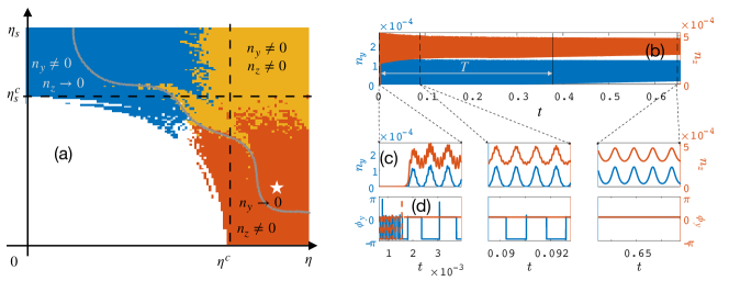
Figure 6: (a) Dynamical phase diagram with three possible self-organized phases in blue, yellow, and orange. Different phases are distinguished from the dynamics of the two cavity fields $\langle a_{y}\rangle$ and $\langle a_{z}\rangle.$ (b) Time evolution of the occupation number for the two cavity modes, for parameters marked with a star in panel (a). (c) Zoom on the dynamics of the photon number and (d) phase at the beginning, middle, and end of time evolution in panel (b). Time is given in seconds, see main text. Here we fix $\omega_{y}=\omega_{z}=5\kappa,$ $\omega_{s}=\omega_{0}/4,$ $\mu=0.75.$

V Probing dynamics with the two cavity fields

We now discuss the different dynamical regimes arising from the interplay of $H_{s}$ and $H$. We show how the auxiliary cavity field dynamics are directly linked with spin precession and entanglement entropy oscillations, facilitating continuous monitoring of the system’s dynamics.

V.1 Dynamical phase diagram

By tuning the two couplings, $\eta$ (spin-momentum) and $\eta_{s}$ (momentum) below and above criticality, we generate the complete diagram of dynamical responses, reported in Fig. 6(a). We initialize the system in the normal state and then fast ramp it at certain values of the couplings [cf. Appendix C].

As order parameters, we consider the mean field expectation values of two cavity fields, $\langle a_{y}\rangle$ and $\langle a_{z}\rangle.$ The choice is convenient for two reasons. Firstly, typical experiments operate in a regime where cavity detunings, $\omega_{y,z},$ and decay rates, $\kappa$, are a few orders of magnitude larger than atomic energy scales Baumann et al. (2010); Ferri et al. (2021); Dogra et al. (2019); Mivehvar et al. (2021). Consequently, one can adiabatically eliminate the cavity modes since on timescales $\propto 1/\kappa$ they approach the steady state values $\langle a_{y}\rangle\approx-2\eta_{s}(\langle J_{01}^{x}\rangle+\langle J_{23}^{x}\rangle)/(\omega_{y}-i\kappa)$, $\langle a_{z}\rangle\approx-2\eta(\langle S_{03}^{x}\rangle+\langle S_{12}^{x}\rangle)/(\omega_{z}-i\kappa)$ Damanet et al. (2019). Thus, the cavity fields $\langle a_{y}\rangle$ and $\langle a_{z}\rangle$ offer direct information about momentum $\langle J^{x}\rangle$ and spin-momentum $\langle S^{x}\rangle$ coherences in the system. Notice that the naïve elimination of the cavity field at the level of the generator of dynamics would result in a lack of relaxation, which is an artifact (in the Dicke model, the decay appears at the higher order of perturbation theory; see Refs.Jäger et al. (2022); Ferri et al. (2021); Keeling et al. (2010) for a comprehensive discussion). Indeed, in order to extract the dynamical responses in Fig. 6, we adopt a Redfield master equation approach Damanet et al. (2019); Jäger et al. (2022); the corresponding equations of motion are reported in Appendices B, C.

The second reason to use cavity fields as order parameters is their experimental accessibility. Using heterodyne detection Brennecke et al. (2013), which gives access to the magnitude and phase of the cavity fields, it is possible to conduct continuous non-destructive measurements of the system. In contrast, imaging the condensate’s spin and density distribution constitutes a destructive measurement, requiring numerous experiment repetitions to reconstruct dynamics.

The system exhibits a variety of self-organization transitions, distinguishable by the dynamics of the cavity fields $\langle a_{y}\rangle$ and $\langle a_{z}\rangle.$ Firstly, when both couplings are smaller than the critical ones [white region in Fig. 6(a)], the system remains in the normal state with zero occupation of the cavity fields. In terms of atomic degrees of freedom, the internal atomic spin precesses with the frequency $2\omega_{s}$ and amplitude given by $\sqrt{1/4-\langle\mathcal{T}^{z}\rangle^{2}}=\sqrt{\mu(1-\mu)}$.

By increasing $\eta$ above the critical value and keeping $\eta_{s}<\eta_{s}^{c}$, the system undergoes a phase transition to the SR phase, associated with breaking of the $\mathbb{Z}_{2}$ symmetry of $H$ [cf. Eq. (2)]. The occupation of the cavity mode $\langle a_{z}\rangle,$ together with the pseudo-spin $\langle S^{x}\rangle$ become non-zero [see red region in Fig. 6(a)]. On the other hand, according to the transformation (12), this spontaneous symmetry breaking also induces explicit symmetry breaking in $H_{s}$ [Eq. (7)], namely, the interaction term gains a phase $\pm(\phi_{1}-\phi_{3}).$ As a consequence, the pseudo-spin $\langle J^{x}\rangle$ starts precessing with a zero time average, resulting in periodic development of $\langle a_{y}\rangle\propto\langle J^{x}\rangle.$ In this way, subsystem (7) experiences superradiance from the interaction with the subsystem (2); otherwise, since $\eta_{s}<\eta_{s}^{c}$, the pseudo-spin $\langle J^{x}\rangle$ together with the cavity field $\langle a_{y}\rangle$ remain in the normal state.

In the experiment, this dynamical phase can be discerned by measuring both the photon number and phase of the two cavity fields, as illustrated in Fig. 6(b-d). Following the fast ramp at $t=0$, the observable $n_{z}=\langle a_{z}^{\dagger}a_{z}\rangle$ approaches a non-zero value. Simultaneously, the photon number of the second mode, denoted as $n_{y}=\langle a_{y}^{\dagger}a_{y}\rangle$, undergoes oscillations, transitioning from zero to a finite value. At each instance when $n_{y}$ returns to zero, the phase $\phi_{y}=\arg\left(\langle a_{y}\rangle\right)$ undergoes a discrete shift of $\pi$, signifying that $\langle a_{y}\rangle$ undergoes a sign reversal, as shown in Fig. 6(c,d). Note that depending on parameters, such a regime with the zero-averaged $\langle a_{y}\rangle$ and periodic jumps of $\phi_{y}$ can take finite time, which we denote $T$ in Fig. 6(b). In the following Section, we relate $T$ with the possibility of non-invasive continuous monitoring of the entanglement dynamics.

In the regime where the field $\langle a_{y}\rangle$ oscillates with zero average, the precession frequency of the pseudo-spin $\langle J^{x}\rangle$ can be calculated as the inverse of the time interval over which the phase of $\langle a_{y}\rangle$ changes by $2\pi$. Simultaneously, the amplitude of $\langle J^{x}\rangle$ oscillations can be deduced from the maximum value of $n_{y}$ during one period, $\operatorname{ampl}(\langle J^{x}\rangle)=[\max(n_{y})(\omega_{y}^{2}+\kappa^{2})]^{1/2}/(2\eta_{s})$.

The time evolution shown in Fig. 6(b-d) is not unique but depends on the phase that is initially imprinted in the boson $c_{i}$ (spin $\Sigma_{ij}$) operators. Different initial conditions can lead to dephasing and variations in the amplitudes and frequencies for different observables due to the nonlinear nature of the problem. However, as we have checked numerically, the oscillatory behavior in Fig. 6(c-d) is generic for different realizations of the initial conditions, meaning one can observe oscillations of the magnitude of the cavity fields and also periodic jumps of the phase of the auxiliary cavity field.

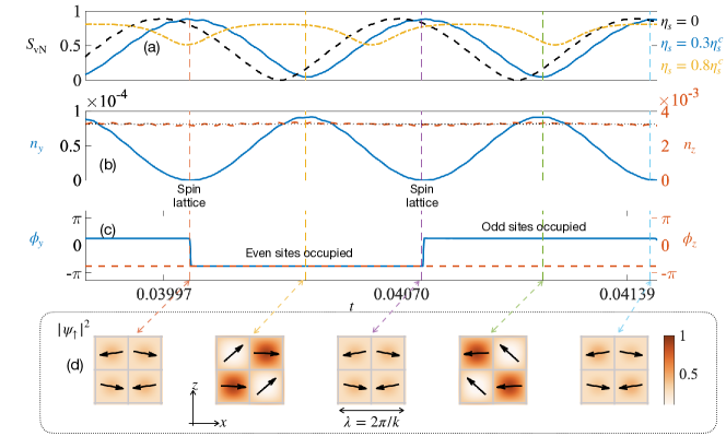
Figure 7: (a) Dynamics of the entanglement entropy, (b) occupation of the cavity modes, (c) phases of the cavity fields, and (d) real space density in the red region in the phase diagram. The black line in panel (a) corresponds to the $\eta_{s}=0$ case, while red and blue lines correspond to the dynamics with non-zero $\eta_{s}\ll\eta_{s}^{c}.$ From oscillations of the cavity field phase $\phi_{y},$ one can recover the structure of the real-space checkerboard lattice: when $\phi_{y}>0$ odd sites are occupied, and when $\phi_{y}<0$ even sited are more occupied. The $n_{y}=0$ case corresponds to the maximally entangled state in which the checkerboard is formed by the spin rather than the density lattice.

In the opposite limit, when $\eta_{s}>\eta_{s}^{c}$ and $\eta$ is below its critical value [blue region in Fig. 6(a)], the transition to the SR phase takes place in cavity field $\langle a_{y}\rangle$ and pseudo-spin $\langle J^{x}\rangle$, while cavity mode $\langle a_{z}\rangle$ experiences oscillations with zero time-average. These oscillations appear due to the explicit symmetry breaking in Hamiltonian $H$ in Eq. (2) and subsequent precession of the pseudo-spin $\langle S^{x}\rangle.$ Similarly to the previous case, the precession period is equal to the time interval during which $\phi_{z}=\arg(\langle a_{z}\rangle)$ changes by $2\pi,$ and the amplitude of $\langle S^{x}\rangle$ oscillations is $\operatorname{ampl}(\langle S^{x}\rangle)=[\max(n_{z})(\omega_{z}^{2}+\kappa^{2})]^{1/2}/(2\eta)$.

Finally, when both couplings are above the critical ones [see the yellow region in Fig. 6(a)], both cavity modes, $\langle a_{y}\rangle$ and $\langle a_{z}\rangle,$ become non-zero, and the symmetry of both $H_{s}$ in Eq. (7) and $H$ in Eq. (2) are spontaneously broken in a self-consistent way. Here, both cavity fields have fixed phases, while their magnitudes can oscillate while the system approaches a (stationary) steady state.

V.2 Slow relaxation in multi-level Dicke model

The oscillations shown in Fig. 6(b) persist far longer than the operational timescales of the experiment. Below, we discuss the mechanism that induces such prolonged relaxation in the dissipative model (8).

The evolution of energy in the two-level Dicke model during relaxation is given by $\differential\langle E\rangle/\differential t=\kappa\mathcal{D}(\omega_{c}a^{\dagger}a+2\eta(a+a^{\dagger})J^{x})$, which in terms of spin degrees of freedom is proportional to $\differential\langle E\rangle/\differential t\propto\langle J^{x}\rangle\langle J^{y}\rangle.$ In the steady state $\langle J^{y}\rangle=0$ and the system’s energy is constant, indicating that all energy pumped from the external driving fields is completely lost through the dissipation of the cavity mode. However, on its way to stationarity, the spin component $\langle J^{y}\rangle$ oscillates around zero value, which means that with period $2\omega_{0}$ energy is pumped in (negative $\langle J^{y}\rangle$) and out (positive $\langle J^{y}\rangle$) of the system, leading to the relaxation time $\tau=(\omega_{y}^{2}+\kappa^{2})/(\omega_{0}^{2}\kappa)\gg 1/\kappa$ Bhaseen et al. (2012); Keeling et al. (2010).

In contrast, in the four-level model (8), the superradiance in one spin species acts as an ‘effective drive’ for the other, inducing an additional factor that slows down the relaxation. Here, the explicit breaking of the Hamiltonian symmetry results in the generation of non-stationary phases. It happens due to the competing conditions on the phases of the boson fields, $\phi_{0},\ldots,\phi_{3},$ set by $H$ [Eq. (2)] and $H_{s}$ [Eq. (7)]. Relaxation in the four-level model (8) is conditioned from the temporal evolution of phases of the boson operators $\phi_{1,\ldots,3},$ whose interdependence slows down reaching a steady state, as it happens in constrained models Bhore et al. (2023); Valencia-Tortora et al. (2022). Such slow relaxation is crucial for the continuous read-out of the system’s dynamics since spin precession can be easily captured at extensive timescales.

V.3 Read-out

We now relate the dynamics of the auxiliary cavity field $\langle a_{y}\rangle$ to the evolution of both the entanglement entropy $S_{\operatorname{vN}}$ and the condensate’s microscopic degrees of freedom. An instance of such dynamics for parameters as in the red region in Fig. 6 ($\eta_{s}=0.3\eta_{s}^{c}$, $\eta=1.6\eta^{c}$) is shown in Fig. 7. Here, the blue line in panel (a) shows the dynamics of the entanglement entropy, panel (b) the dynamics of the populations of the two cavity modes, panel (c) the dynamics of the phase of two cavity fields, and finally panel (d) shows snapshots of the condensate density at different times. Arrows in panel (d) indicate spin magnetization in the centers of the checkerboard lattice sites.

The oscillations of the photon number $n_{y}=\langle a_{y}^{\dagger}a_{y}\rangle$ [panel(b)] and the phase $\phi_{y}=\arg(\langle a_{y}\rangle)$ [panel (c)] capture precession of the external pseudo-spin $\langle J^{x}\rangle,$ as $\langle a_{y}\rangle\approx-2\eta_{s}(\langle J_{01}^{x}\rangle+\langle J_{23}^{x}\rangle)/(\omega_{y}-i\kappa)$. When the phase of the cavity field changes by $\pm\pi,$ the real space density checkerboard lattice changes its parity [odd or even lattice sites are more occupied, see panel (d)]. Concomitantly, the system reaches the maximum value of the entanglement entropy [panel (a)]. At the same time, the checkerboard lattice with period $\lambda=2\pi/k$ is formed not by modulation of the density but rather by the different orientations of the spin in the centers of even and odd sites.

When the phase of the field $\langle a_{y}\rangle$ gains $\pm\pi$ jump, the spatial density profile changes parity. At the same time, the increase of the photon number $n_{y}$ indicates a decrease of entanglement since the coupling $\eta_{s}$ tends to disentangle spin and momentum, while a decrease of $n_{y}$, on the other hand, indicates the developing of the spin-momentum correlations in the system. In this way, one can capture real-time oscillations of the entanglement entropy from the oscillations of the cavity field $\langle a_{y}\rangle.$

Finally, the fixed phase of the cavity field $a_{z},$ $\phi_{z}=\arg(\langle a_{z}\rangle),$ indicates the spontaneous symmetry breaking in $H$ [cf. Eq. (2)]. In terms of the atomic degrees of freedom, the fixed phase $\phi_{z}$ in panel (c) captures the absence of the mirror symmetry between maximally entangled states, namely for two consecutive maximally entangled states, the spin lattices are exactly the same, without the symmetry under swapping even and odd sites, cf. even panels in Fig. 7(d).

The heterodyne detection of two cavity modes $a_{y}$ and $a_{z}$ enables distinguishing different dynamical phases in the system in a non-destructive way. However, by itself, the coupling to the auxiliary cavity mode can change the steady state properties and, more importantly in the context of this paper, change the entanglement of the system compared to the single-mode model. In this regard, it is important to separate a range of couplings for which utilizing additional polarization preserves most of the entanglement and, at the same time, is sufficient to perform measurements. We dedicate the next Section to this aim.

VI Entanglement in the two photon fields model

In this Section, we revisit the system’s various dynamical responses in terms of spin-momentum entanglement generation when both cavity modes contribute to the dynamics and identify parameter ranges suitable for non-invasive monitoring of the dynamics of collective observables. We show criteria to determine the range of parameters for which the auxiliary cavity mode creates a minimal backaction on the system’s dynamics. For all extra details, we refer the reader to Appendix G.

The entanglement properties of the system are conditioned from the competition between $\eta$ [which couples spin-momentum pseudo-spins with cavity mode $a_{z}$ and tries to entangle spin and momentum] and $\eta_{s}$ [which couples momentum pseudo-spins $J$ with the cavity field $a_{y}$ and tends to maintain spin and momentum separable]. Fig. 8 shows numerical data on the maximal entanglement $\max(S_{\operatorname{vN}})$ as a function of these ‘spin-momentum’ $\eta$ and ‘momentum’ $\eta_{s}$ couplings. Here, we maintain the same parameters as those in the phase diagram of Fig. 6(a). The plot shows that increasing $\eta$ induces stronger correlations between spin and momentum, while $\eta_{s}$ acts as a disentangling agent.

The interplay between $\eta$ and $\eta_{s}$ can significantly alter not only the $\max(S_{\operatorname{vN}})$ but also the steady-state properties of the system along with the evolution of the $S_{\operatorname{vN}}$ compared to the $\eta_{s}=0$ case. Fig. 7(a) shows the evolution of the $S_{\operatorname{vN}}$ for weak, strong, and zero coupling $\eta_{s}$ to the auxiliary mode $a_{y}$. Compared to the unprobed model ($\eta_{s}=0$, black line), for weak values the photon-matter coupling slightly modifies the steady state and entanglement dynamics ($\eta_{s}=0.3\eta_{s}^{c}\ll\eta_{s}^{c}$, blue line), while for strong values, it can alter dynamics of the $S_{\operatorname{vN}}$ significantly ($\eta_{s}=0.8\eta_{s}^{c}$, yellow line). These regimes can be distinguished from the dynamics of the auxiliary field. For weak couplings, the read-out is non-invasive, and the auxiliary field oscillates with the zero time average for timescales that significantly exceed the operational timescale of the experiment ($t_{\operatorname{op}}\propto 0.01$ s). In the experiment, these oscillations correspond to periodic changes in the phase of the auxiliary field. In the strong coupling regime, the read-out procedure is invasive, and the phase of the auxiliary field becomes fixed after some time, $T,$ which is comparable with the operational timescale of the experiment. At this time, the explicitly broken symmetry of the Hamiltonian is restored, and the system starts evolving toward the SR state for both cavity fields.

The restoration of the symmetry indicates the change in the steady state and, thus also entanglement properties of the system. Because of this, for non-destructive probing of the dynamics, it would be convenient to work in a parameter regime where $T/t_{\operatorname{op}}\to\infty.$ Our numerics suggests that $T\propto\exp(\eta_{s}-\eta_{s}^{c}),$ revealing that symmetry restoration occurs more rapidly as the coupling to the auxiliary mode approaches the critical threshold, cf. Appendix G. As such, for non-destructive monitoring dynamics, it is essential to maintain the coupling to the auxiliary field significantly below the critical value.

Combining the information on relaxation timescales with the amount of entanglement generated in Fig. 8 (see Appendix C for more details), it appears that in the limit of $\eta\gg\eta^{c}$ and $\eta_{s}\ll\eta_{s}^{c}$ highly entangled states are prepared, while the system keeps oscillating for long times, facilitating the reconstruction of oscillations of the entanglement entropy by measuring the auxiliary cavity field $\langle a_{y}\rangle$ (cf. Fig. 7). On the other hand, in the part of the phase diagram dominated by the coupling $\eta_{s},$ there is no strong entanglement, albeit $\eta$ can still induce short-lived spin-momentum correlations.

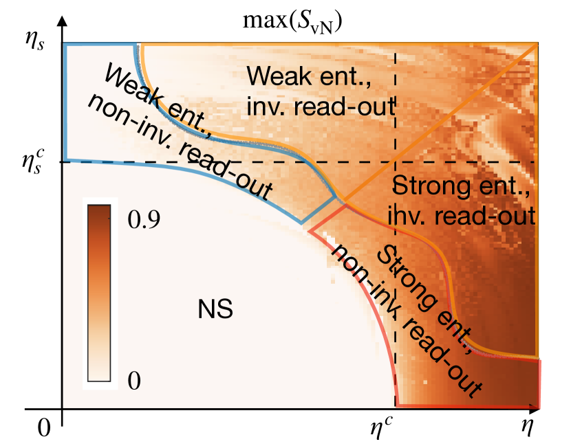
Figure 8: Maximum value of the entanglement entropy at late times as a function of the couplings $\eta$ and $\eta_{s}.$ Parameters are the same as in Fig. 6. The cartoon in Fig. 1(c) is sketched from the data of this figure.

By adjusting experimentally accessible parameters, such as couplings $\eta,~{}\eta_{s}$ and detuning $\omega_{s}$, one can tune the amplitude, time-average, and oscillation frequency of the entanglement entropy, thereby dynamically controlling the correlation between spin and momentum. In principle, the simplest approach is to set $\omega_{y}/\kappa\to 0$, which ensures that pseudo-spins do not receive any feedback from $a_{y}$, and thus, all entanglement properties are solely determined by light-matter interactions contained in $H$. In this case, the dissipation induces a phase shift of the auxiliary cavity field, $\phi_{\kappa}^{y}=\tan^{-1}\left(-\kappa/\omega_{y}\right)=\pi/2$ Dogra et al. (2019), making it imaginary, $\langle a_{y}\rangle+\langle a_{y}^{\dagger}\rangle=0,$ and reducing backaction of the field $a_{y}$ on the $H$, see Appendix G. However, the effective model with $H_{\operatorname{tot}}$ [Eq. (8)] breaks down for these extreme conditions because the many-body description of the model, in this case, requires taking into account higher momentum modes.

A more practical scenario is when the frequency of the auxiliary cavity photon $\omega_{y}$ is much higher than $\kappa.$ In this case, it is easier to maintain $\eta_{s}/\eta_{s}^{c}\ll 1,$ but have cavity occupations $n_{y}$ large enough to continuously measure the collective momentum.

Furthermore, sizable stationary entanglement can be preserved when $\omega_{s}=0$. Here, the Hamiltonian gains additional symmetry under the exchange of ground and excited momentum levels of two spin sub-levels, $(\ket{0},\ket{1})\leftrightarrow(\ket{2},\ket{3})$. In this case, the induced as a result of the explicit symmetry breaking phase $\pm(\phi_{1}-\phi_{3})$ does not evolve in time, and the explicitly broken symmetry can not be restored, see Appendix G for comprehensive discussion. For $\omega_{s}=0$ the maximal and time-averaged amount of entanglement remains similar to the one generated with one main cavity mode [see Fig. 3(a)], besides a small dressing induced by $\eta_{s}$.

VII CONCLUSIONS AND OUTLOOK

In this work, we have presented an experimentally feasible cavity QED platform featuring an effective four-level atomic description and shown that it manifests two intertwined self-organization transitions. This system serves as a minimal model wherein spontaneous symmetry breaking occurs in an all-to-all interacting spin model, concomitant with the formation of tunable spin-momentum entanglement. The controlled leakage of intra-cavity photons plays an important stabilization role, as the resulting dissipative dynamics facilitate convergence towards the target entangled state in a manner resilient to imperfections in the system’s couplings or initial state preparation. Extending the coupling scheme with an auxiliary cavity mode gives rise to persistent oscillations (due to explicit symmetry breaking) and facilitates real-time monitoring of the system dynamics, in particular, as a proxy for entanglement.

The tunable parameters of our model facilitate a straightforward extension to spin-exchange interactions, akin to the Tavis-Cummings model Soriente et al. (2018); Ferri et al. (2021); Kirton and Keeling (2018). An interesting avenue for exploration lies in understanding how quantum correlations between spin and momentum can be continuously tuned as one transitions between the Tavis-Cummings and Dicke limits considered here.

We should note that a relation between multi-level atoms and entanglement has been previously reported both in cavity QED systems Piñeiro Orioli et al. (2022); Orioli and Rey (2020); Hotter et al. (2023); Sundar et al. (2023) and photonic waveguides Asenjo-Garcia et al. (2019); Manzoni et al. (2017); Masson and Asenjo-Garcia (2022); Sierra et al. (2022); Tabares et al. (2023). In these cases, entangled states can be hosted within the sub-radiant subspaces of the multi-level atoms, with level degeneracies being crucial for the build-up of quantum correlations. The mechanism is markedly different from ours, although considering a combination of the two setups could naturally lead to further interesting developments.

Taking a broader perspective, one could investigate how different dynamical phases of matter routinely engineered in cavity QED would morph, when both spin and momentum degrees of freedom are optically addressed. Our analysis has focused on the superradiant phase transition as a paradigmatic case, but it would be intriguing to see whether entanglement properties of spin-momentum hybridized states can be manipulated as a response to periodic drives Skulte et al. (2021); Kongkhambut et al. (2021); Reilly et al. (2023) or in the context of dissipative-induced phase transitions Dogra et al. (2019); Kongkhambut et al. (2022); Klinder et al. (2015); Buča and Jaksch (2019); Soriente et al. (2018).

Appendix A Derivation of the Hamiltonian

In this Appendix, we present a derivation of Hamiltonian $H_{\operatorname{tot}}$ for a setup depicted in Figs. 2 and 5. The derivation of the Hamiltonian $H$ or $H_{s}$ can be obtained by setting $E_{s}=0$ or $E_{b}=E_{r}=0$ below respectively.

We start with the general Hamiltonian for the light-matter interaction problems, which reads

$$H_{\operatorname{tot}}=H_{c}+H_{a}+H_{\text{int}},$$ (14)

where $H_{c}$ governs dynamics of the cavity mode, $H_{a}$ is single-atom Hamiltonian and $H_{\text{int}}$ describes interaction between atom and the cavity. We specify the explicit form of $H_{c},$ $H_{a}$ and $H_{\text{int}}$ in the considered setup and show under which assumptions the low-energy physics of the model can be simulated by Eq. (8).

We immerse ⁸⁷Rb atoms inside an optical cavity oriented along the $\mathbf{e}_{x}$ axis. The cavity has a single relevant frequency $\omega_{c}=2\pi\cdot 382.04685\text{ THz}$ with a decay rate of $\kappa\sim 2\pi\cdot 1.25\text{ MHz}$, and two polarizations $\mathbf{e}_{y}$ and $\mathbf{e}_{z}.$ We represent two corresponding cavity polarization modes by operators ${a}_{{y}}$ and ${a}_{{z}},$ respectively. The cavity Hamiltonian reads

$$H_{c}=\hbar\omega_{y}a_{y}^{\dagger}a_{y}+\hbar\omega_{z}a_{z}^{\dagger}a_{z}.$$ (15)

We apply a classical pump field with a Gaussian profile in the transverse direction, $\mathbf{e}_{x}$, and a standing wave profile in the longitudinal direction, $\mathbf{e}_{z}$, which is implemented using a retroreflective mirror. We consider a dispersive regime, in which pumping frequency is chosen out-of-resonance with the electron transition $5^{2}S_{1/2}\to 5^{2}P_{1/2},~{}5^{2}P_{3/2}$. In this case, excited atomic states can be eliminated, and the resulting atomic Hamiltonian within the $F=1$ hyperfine manifold of the $5^{2}s_{1/2}$ level reads

$$H_{a}=\frac{\mathbf{p}^{2}}{2M}+V_{\text{ext}}+\sum_{F,m_{F}}\hbar\omega_{F,m_{F}}|F,m_{F}\rangle\langle F,m_{F}|,$$ (16)

where $\mathbf{p}$ is the momentum of the atom, $M$ is the atomic mass, $V_{\text{ext}}$ describes an external trapping potential, and the energy of atomic level $|F,m_{F}\rangle$ is $\hbar\omega_{F,m_{F}}.$ The sum in the last terms runs over all atomic levels in $F=1$ manifold. We apply a strong magnetic field $\mathbf{B}=-B\mathbf{e}_{z}$ along $z$ direction, which induces first and second-order Zeeman splitting between levels with different magnetic numbers $m_{F}.$ Introducing internal spin operator $\mathbf{F}=\left(F^{x},F^{y},F^{z}\right)$, the atomic part of the Hamiltonian can be rewritten

$$H_{a}=\frac{\mathbf{p}^{2}}{2M}+V_{\text{ext}}+\hbar\omega_{z}^{(1)}F^{z}+\hbar\omega_{z}^{(2)}F^{z2},$$ (17)

where $\omega_{z}^{(1)}<0$ and $\omega_{z}^{(2)}>0$ are the first and the second order Zeeman splittings.

The atoms are neutral and are much smaller than the wavelength of the optical light fields so that the light-matter interaction can be described in the dipole approximation

$${H}_{\text{int}}=-{\mathbf{d}}_{\text{lab}}{\mathbf{E}}_{\text{lab}},$$ (18)

where the atomic dipole operator can be expanded in terms of the atom’s internal states

$${\mathbf{d}}_{\text{lab}}=\sum_{e,g}\mathbf{d}_{eg}\ket{e}\bra{g}+\text{h.c.},\quad\mathbf{d}_{eg}=\bra{e}{\mathbf{d}}\ket{g}.$$ (19)

The total optical field $\mathbf{E}_{\text{lab}}$ is the sum of the classical pump field, ${\mathbf{E}}_{p}\left({\mathbf{r}}\right)$, and the cavity field, ${\mathbf{E}}_{c}\left({\mathbf{r}}\right)$. The classical pump field has a Gaussian profile in the transverse direction ($\mathbf{e}_{x}$) and a standing wave profile in the longitudinal direction ($\mathbf{e}_{z}$):

$$\mathbf{E}_{p}\left({\mathbf{x}}\right)=\mathbf{e}_{p}\sum_{\beta=b,r,g}\frac{E_{\beta}}{2}f_{\beta}\left({\mathbf{r}}\right)e^{-i\omega_{\beta}t}+\text{h.c.},$$ (20)

where the linear polarization of the pumping field $\mathbf{e}_{p}=\cos\left(\varphi\right)\mathbf{e}_{y}+\sin\left(\varphi\right)\mathbf{e}_{x}.$ We fix $\phi=\pi/2,$ which sets the coupling between the atoms and the real quadrature of the cavity field below . The mode function for each sideband is $f_{\beta}\left({\mathbf{r}}\right)=\exp\left({-\left({2{x}^{2}}/{w_{x}^{2}}-{2{y}^{2}}/{w_{y}^{2}}\right)}\right)\cos\left(k_{\beta}{z}\right)$. The widths of the transverse Gaussian profile are approximately $\omega_{x},\omega_{y}\approx 25\text{ }\mu\text{m}$. The wave-vectors are $k_{\beta}={\omega_{\beta}}/{c}\approx{\omega_{p}}/{c}$ with $c$ denoting speed of light. Here we consider three laser drivers $\beta=b,r,s,$ with the sideband frequencies $\omega_{b(r)}$ such that detunings $\delta\omega_{\beta}=\omega_{\beta}-\omega_{p}$ are chosen to correspond to the differences in first-order Zeeman shifts (in the $F=1$ ground state manifold). In contrast, the third detuning is set to be zero, $\omega_{s}=(\omega_{b}+\omega_{r})/2=\bar{\omega}$. In this case, different driving schemes operate with the same momentum states. We limit our consideration to the case when $E_{b}=E_{r}\neq E_{s}.$

The cavity field TEM00 mode of a Fabry-Perot cavity has a standing wave profile in the transverse direction ($\mathbf{e}_{x}$) and a Gaussian profile in the other two directions:

$$\mathbf{E}_{c}\left({\mathbf{x}}\right)=\mathbf{e}_{{y}}E_{c}g_{{y}}\left({\mathbf{r}}\right){a}_{{y}}+\mathbf{e}_{{z}}E_{c}g_{{z}}\left({\mathbf{r}}\right){a}_{{z}}+\text{h.c.}$$ (21)

where the mode functions are $g_{{y},{z}}\left({\mathbf{r}}\right)=\exp\left(-({2\left({y}^{2}+{z}^{2}\right))/{w_{c}^{2}}}\right)\cos\left(k_{c}{x}\right)$ with the Gaussian profile having a width of approximately $w_{c}\approx 25\text{ }\mu\text{m}$. The wave-vectors are $k_{{y},{z}}\approx k_{c}=\omega_{c}/{c}$.

As we are working in the dispersive regime, the excited atomic states can be eliminated using the Schrieffer-Wolff Haq et al. (2019) transformation ${H}\rightarrow e^{{S}}{H}e^{-{S}}$, $\left[{S},{H}_{0}\right]=-{H}_{\text{int}}$, which results in the low-energy Hamiltonian

$${H}_{0}=\frac{{\mathbf{p}}^{2}}{2M}+V_{\text{ext}}+\hbar\omega^{(1)}{F}^{z}+\hbar\omega^{(2)}{F}^{2}+\hbar\omega_{c}^{{y}}a_{{y}}^{\dagger}a_{{y}}+\hbar\omega_{c}^{{z}}a_{{z}}^{\dagger}a_{{z}}$$ (22)

$${H}_{\mathrm{int}}^{s}=\alpha_{s}f^{2}({\mathbf{r}})\left|\sum_{\beta}\frac{E_{\beta}}{2}e^{i\delta\omega_{\beta}t}\right|^{2}+\alpha_{s}\left|E_{c}\right|^{2}g^{2}({\mathbf{r}})\left({a}_{{y}}^{\dagger}{a}_{{y}}+{a}_{{z}}^{\dagger}{a}_{{z}}\right)$$

$$+\alpha_{s}\overbrace{\left(\mathbf{e}_{p}\cdot\mathbf{e}_{{y}}\right)}^{=1}f({\mathbf{r}})g({\mathbf{r}})\sum_{\beta}\frac{E_{\beta}}{2}\left(e^{i\omega_{\beta}t}{a}_{{y}}+e^{-i\omega_{\beta}t}{a}_{{y}}^{\dagger}\right)+\alpha_{s}\overbrace{\left(\mathbf{e}_{p}\cdot\mathbf{e}_{{z}}\right)}^{=0}f({\mathbf{r}})g({\mathbf{r}})\sum_{\beta}\frac{E_{\beta}}{2}\left(e^{i\omega_{\beta}t}{a}_{{z}}+e^{-i\omega_{\beta}t}{a}_{{z}}^{\dagger}\right)$$

$${H}_{\mathrm{int}}^{v}=-i\frac{\alpha_{v}}{2F}g({\mathbf{r}})f({\mathbf{r}})\sum_{\beta}\frac{E_{c}E_{\beta}}{2}\left[\left({a}_{{y}}e^{i\omega_{\beta}t}-{a}_{{y}}^{\dagger}e^{-i\omega_{\beta}t}\right)\overbrace{\left(\mathbf{e}_{p}\times\mathbf{e}_{{y}}\right)}^{=0}\cdot{\mathbf{F}}+\left({a}_{{z}}e^{i\omega_{\beta}t}-{a}_{{z}}^{\dagger}e^{-i\omega_{\beta}t}\right)\overbrace{\left(\mathbf{e}_{p}\times\mathbf{e}_{{z}}\right)}^{=\mathbf{e}_{x}}\cdot{\mathbf{F}}\right]$$

$$-\underbrace{i\frac{\alpha_{v}}{2F}E_{c}^{2}g^{2}({\mathbf{r}})\left({a}_{{y}}^{\dagger}{a}_{{z}}-{a}_{{z}}^{\dagger}{a}_{{y}}\right)\left(\mathbf{e}_{{y}}\times\mathbf{e}_{{z}}\right)\cdot\overbrace{{\mathbf{F}}}^{\propto e^{\pm i\omega t}}}_{=0,\text{ because of resonance conditions }}$$

For the transitions in multi-level atoms, it is convenient to account for selection rules using polarizabilities. In the above equation, $\alpha_{s,v}$ are scalar and vector polarizabilities of the atoms, which are components of the rank-2 tensor $\alpha_{i,j}=\sum_{g,g^{\prime}}\sum_{e}\langle g|d_{i}|e\rangle\langle e|d_{j}^{\dagger}|g^{\prime}\rangle|g\rangle\langle g^{\prime}|/(\hbar\Delta_{e})$ defined as follows ${\alpha}_{\mathrm{s}}=\alpha_{\mathrm{s}}{\mathrm{I}}\delta_{ij}$, ${\alpha}_{\mathrm{v}}=-i\frac{\alpha_{\mathrm{v}}}{2\mathrm{~{}F}}\epsilon_{ijk}{F}_{k}.$ The sum runs over all allowed transitions (see Ref. Steck (2021)), $d_{i}$ is the component of the atomic dipole moment, and the detuning of the driving field from the resonance frequency is $\Delta_{e}\approx\omega_{p}-\omega_{e}.$

Finally, we move to a frame rotating with the classical pump frequency: ${H}_{\text{lab}}\rightarrow{H}={U}_{p}^{\dagger}{H}_{\text{lab}}{U}_{p}-{H}_{p}$ where ${U}_{p}=\exp(-{i{H}_{p}t}/{\hbar})$ and ${H}_{p}=\sum_{e}\hbar\omega_{p}\ket{e}\bra{e}+\hbar\omega_{p}\left({a}_{{y}}^{\dagger}{a}_{{y}}+{a}_{{z}}^{\dagger}{a}_{{z}}\right)$. The rotating-wave approximation brings us to the time-independent single-body Hamiltonian

$$H_{\operatorname{tot}}=H_{a}+H_{c}+H_{s}+H_{v},$$ (23)

$$H_{a}=\frac{\mathbf{p}^{2}}{2M}+V_{\text{ext}}+\hbar\delta^{(1)}F^{z}+\hbar\omega^{(2)}F^{z2},$$ (24)

$$H_{c}=-\Delta_{y}a_{y}^{\dagger}a_{y}-\Delta_{z}a_{z}^{\dagger}a_{z},$$ (25)

$$H_{s}=\frac{\alpha_{s}}{4}f^{2}(\mathbf{r})\left(E_{s}^{2}+E_{b}^{2}+E_{r}^{2}\right)+\alpha_{s}E_{0}^{2}g^{2}(\mathbf{r})\left(a_{y}^{\dagger}a_{y}+a_{z}^{\dagger}a_{z}\right)+\frac{\alpha_{s}}{2}f(\mathbf{r})g(\mathbf{r})E_{0}E_{s}(a_{y}+a_{y}^{\dagger})$$ (26)

$$H_{v}=\frac{\alpha_{v}}{4}E_{0}E_{b(r)}f(\mathbf{r})g(\mathbf{r})(a_{z}+a_{z}^{\dagger})F^{x}$$ (27)

where $\delta^{(1)}=\omega_{z}^{(1)}+(\omega_{b}-\omega_{r})/2,$ $\Delta_{y,z}=\bar{\omega}-\omega_{y,z}<0.$ We have also applied a transformation $a_{z}\to ia_{z}$ to get rid of the minus sign in $H_{v}.$ The first term in $H_{s}$ describes the attractive potential created by the transverse driving fields, the second term describes the dispersive shift to the cavity detuning, and the last term produces the Bragg transition within the same atomic level. The vectorial interaction describes the Raman process when the transition happens between nearing sub-levels of the ground-state manifold.

Let us consider a case when the magnetic field is strong. Specifically, let the second order Zeeman shift $\omega^{(2)}\propto 1~{}\text{MHz},$ and thus the resonant conditions for transition $m_{F}=1\leftrightarrow m_{F}=0$ are out-of-resonance for transition $m_{F}=0\leftrightarrow m_{F}=-1.$ In this case, if we prepare the initial state as a mixture of particles at levels with $m_{F}=1,0,$ the dynamics will be restricted to these two atomic levels for the typical operational times of the experiment. In this case, we can limit our consideration to the dynamics between two neighboring spin levels, defining the many-body spinor field operator

$$\Psi(\mathbf{r})=(0,\psi_{\uparrow},\psi_{\downarrow})^{T},$$ (28)

which satisfies standard bosonic commutation relations $[\psi_{\sigma}(\mathbf{r}),\psi_{\sigma^{\prime}}^{\dagger}(\mathbf{r}^{\prime})]=\delta_{\sigma,\sigma^{\prime}}\delta(\mathbf{r}-\mathbf{r}^{\prime}),$ $[\psi_{\sigma}(\mathbf{r}),\psi_{\sigma^{\prime}}(\mathbf{r}^{\prime})]=0,$ where $\sigma,\sigma^{\prime}=\uparrow,\downarrow.$ The $N-$body Hamiltonian reads

$$H_{\operatorname{tot}} =H_{c}+\int\differential\mathbf{r}\Psi^{\dagger}(\mathbf{r})\left(H_{a}+H_{s}+H_{v}\right)\Psi(\mathbf{r})=$$ (29)

$$=H_{c}+\int\differential\mathbf{r}\left[\frac{\alpha_{s}}{4}\left(E_{s}^{2}+E_{b}^{2}+E_{r}^{2}\right)f^{2}(\mathbf{r})+\alpha_{s}E_{0}^{2}\left(a_{y}^{\dagger}a_{y}+a_{z}^{\dagger}a_{z}\right)g^{2}(\mathbf{r})\right]\left(\psi^{\dagger}_{\uparrow}(\mathbf{r})\psi_{\uparrow}(\mathbf{r})+\psi^{\dagger}_{\downarrow}(\mathbf{r})\psi_{\downarrow}(\mathbf{r})\right)$$

$$+\int\differential\mathbf{r}\psi^{\dagger}_{\uparrow}(\mathbf{r})\left(-\frac{\hbar^{2}\nabla^{2}}{2M}+V_{\mathrm{ext}}\right)\psi_{\uparrow}(\mathbf{r})+\int\differential\mathbf{r}\psi^{\dagger}_{\downarrow}(\mathbf{r})\left(-\frac{\hbar^{2}\nabla^{2}}{2M}+V_{\mathrm{ext}}\right)\psi_{\downarrow}(\mathbf{r})+$$

$$+\frac{\hbar\delta^{(1)}}{2}\int\differential\mathbf{r}\left(\psi^{\dagger}_{\uparrow}(\mathbf{r})\psi_{\uparrow}(\mathbf{r})-\psi^{\dagger}_{\downarrow}(\mathbf{r})\psi_{\downarrow}(\mathbf{r})\right)+\frac{\hbar\omega^{(2)}}{4}\int\differential\mathbf{r}\left(\psi^{\dagger}_{\uparrow}(\mathbf{r})\psi_{\uparrow}(\mathbf{r})+\psi^{\dagger}_{\downarrow}(\mathbf{r})\psi_{\downarrow}(\mathbf{r})\right)$$

$$+\frac{\alpha_{s}}{2}E_{0}E_{s}\left(a_{y}+a_{y}^{\dagger}\right)\int\differential\mathbf{r}f(\mathbf{r})g(\mathbf{r})\left(\psi^{\dagger}_{\uparrow}(\mathbf{r})\psi_{\uparrow}(\mathbf{r})+\psi^{\dagger}_{\downarrow}(\mathbf{r})\psi_{\downarrow}(\mathbf{r})\right)+$$

$$+\frac{\alpha_{v}}{8}E_{0}E_{b(r)}\left(a_{z}+a_{z}^{\dagger}\right)\int\differential\mathbf{r}f(\mathbf{r})g(\mathbf{r})\left(\psi^{\dagger}_{\uparrow}(\mathbf{r})\psi_{\downarrow}(\mathbf{r})+\psi^{\dagger}_{\downarrow}(\mathbf{r})\psi_{\uparrow}(\mathbf{r})\right).$$

To derive a Dicke model, we should further restrict the Hilbert space of the model by considering only the two lowest momentum states of the model for both spinor components. In this approximation the many-body wave function reads $\Psi(\mathbf{r})=(0,\phi_{0}(\mathbf{r})c_{0}+\phi_{1}(\mathbf{r})c_{1},\phi_{0}c_{2}(\mathbf{r})+\phi_{1}(\mathbf{r})c_{3})^{T}.$ Here, $c_{i}$ are the annihilation operators of the corresponding atomic modes, $[c_{i},c_{j}^{\dagger}]=\delta_{i,j},~{}[c_{i},c_{j}]=0$, and $\phi_{1}(\mathbf{r})=\mathcal{N}\cos kx\cos kz\phi_{0}(\mathbf{r}),$ where $\mathcal{N}$ accounts for the correct normalization. In this notation, operators $c_{0}$ and $c_{2}$ correspond to the ground momentum states, while operators $c_{1}$ and $c_{2}$ correspond to the excited momentum states. After integrating over all space, the many-body Hamiltonian reads

$$H_{\operatorname{tot}}= -\hbar\Delta_{y}a_{y}^{\dagger}a_{y}+\hbar\omega_{0}\left({c}_{1}^{\dagger}{c}_{1}+{c}_{3}^{\dagger}{c}_{3}\right)+\hbar\eta_{s}\left({a}_{{y}}+{a}_{{y}}^{\dagger}\right)\left({c}_{0}^{\dagger}{c}_{1}+{c}_{1}^{\dagger}{c}_{0}+{c}_{2}^{\dagger}{c}_{3}+{c}_{3}^{\dagger}{c}_{2}\right)$$ (30)

$$-\hbar\Delta_{z}a_{z}^{\dagger}a_{z}+\hbar\omega_{s}\left({c}_{2}^{\dagger}{c}_{2}+{c}_{3}^{\dagger}{c}_{3}\right)+\hbar\eta\left({a}_{{z}}+{a}_{{z}}^{\dagger}\right)\left({c}_{1}^{\dagger}{c}_{2}+{c}_{0}^{\dagger}{c}_{3}+{c}_{2}^{\dagger}{c}_{1}+{c}_{3}^{\dagger}{c}_{0}\right),$$

where the cavity detuning is dressed via the dynamic (dispersive) shift $\Delta_{y,z}=\Delta_{y,z}-\alpha_{s}E_{0}^{2}N\mathcal{I}/\hbar$, the level splitting between ground and excited momentum states is equal $\omega_{0}=2\omega_{\text{rec}}$, $\omega_{s}=\delta^{(1)}$, and coupling constants read as follows: $\hbar\eta_{s}={\alpha_{s}}E_{0}E_{s}\mathcal{M}/2$, $\hbar\eta=-{\alpha_{v}}E_{0}E_{b(r)}\mathcal{M}/{4\sqrt{2}}$, where $\mathcal{I}=\int\differential\mathbf{r}g^{2}(\mathbf{r})\phi_{0}^{2}(\mathbf{r}),$ $\mathcal{M}=\int\differential\mathbf{r}f(\mathbf{r})f(\mathbf{r})\psi_{1}(\mathbf{r})\psi_{0}(\mathbf{r})$. We have omitted standing wave potential ${\alpha_{s}}\left(E_{s}^{2}+E_{b}^{2}+E_{r}^{2}\right)\int\differential\mathbf{r}f^{2}(\mathbf{r})\phi_{0}^{2}(\mathbf{r})/4$ above as it only contributes to the higher momentum state and does not qualitatively modify the appearance of the phase transition discussed in the main text in Fig. 6.

Finally, one can introduce pseudo-spin operators according to Eq. (10), which brings the Hamiltonian to the following form:

$$H_{\operatorname{tot}} =\omega_{y}a_{y}^{\dagger}a_{y}+\omega_{0}\left(J_{01}^{z}+J_{23}^{z}\right)+\eta_{s}\left(a_{y}+a_{y}^{\dagger}\right)\left(J_{01}^{+}+J_{23}^{+}+J_{01}^{-}+J_{23}^{-}\right)+$$ (31)

$$+\omega_{z}a_{z}^{\dagger}a_{z}+\omega_{s}\left(S_{12}^{z}+S_{03}^{z}\right)+\eta\left(a_{z}+a_{z}^{\dagger}\right)\left(S_{12}^{+}+S_{03}^{+}+S_{12}^{-}+S_{03}^{-}\right),$$

where we set $\omega_{y,z}=-\Delta_{y,z}>0$ and have normalized the Hamiltonian by $\hbar\omega_{\text{rec}}$ so that $\omega_{0}=2$ above.

Appendix B Equations of motion

In this Appendix, we derive mean-field equations of motion from the Hamiltonian in (31). Note that for the remainder of the Appendices, we omit $\langle\cdot\rangle$ for expectation values of observables for simplicity.

The mean-field equations of motion can be easily derived from the Lindblad master equation (9) and read

$$\dot{a}_{y} =-i(\omega_{y}-i\kappa)a_{y}-i\eta_{s}\left({c}_{0}^{\dagger}{c}_{1}+{c}_{1}^{\dagger}{c}_{0}+{c}_{2}^{\dagger}{c}_{3}+{c}_{3}^{\dagger}{c}_{2}\right)$$ (32)

$$\dot{a}_{z} =-i(\omega_{z}-i\kappa)a_{z}-i\eta\left({c}_{1}^{\dagger}{c}_{2}+{c}_{0}^{\dagger}{c}_{3}+{c}_{2}^{\dagger}{c}_{1}+{c}_{3}^{\dagger}{c}_{0}\right)$$

$$\dot{c}_{0} =-i\eta\left({a}_{z}+{a}_{z}^{\dagger}\right){c}_{3}-i\eta_{s}\left({a}_{y}+{a}_{y}^{\dagger}\right){c}_{1}$$

$$\dot{c}_{1} =-i\omega_{0}{c}_{1}-i\eta\left({a}_{z}+{a}_{z}^{\dagger}\right){c}_{2}-i\eta_{s}\left({a}_{y}+{a}_{y}^{\dagger}\right){c}_{0}$$

$$\dot{c}_{2} =-i\omega_{s}{c}_{2}-i\eta\left({a}_{z}+{a}_{z}^{\dagger}\right){c}_{1}-i\eta_{s}\left({a}_{y}+{a}_{y}^{\dagger}\right){c}_{3}$$

$$\dot{c}_{3} =-i\left(\omega_{s}+\omega_{0}\right){c}_{3}-i\eta\left({a}_{z}+{a}_{z}^{\dagger}\right){c}_{0}-i\eta_{s}\left({a}_{y}+{a}_{y}^{\dagger}\right){c}_{2}$$

In terms of pseudo-spin degrees of freedom (10), the equations of motion take the following form

$$\frac{dJ_{01}^{-}}{dt} =-2i\omega_{0}J_{01}^{-}+2i\eta_{s}\left(a_{y}+a_{y}^{\dagger}\right)J_{01}^{z}+i\eta\left(a_{z}+a_{z}^{\dagger}\right)\left(\mathcal{T}_{13}^{+}-\mathcal{T}_{02}^{-}\right)$$ (33)

$$\frac{dJ_{23}^{-}}{dt} =-2i\omega_{0}J_{23}^{-}+2i\eta_{s}\left(a_{y}+a_{y}^{\dagger}\right)J_{23}^{z}+i\eta\left(a_{z}+a_{z}^{\dagger}\right)\left(\mathcal{T}_{13}^{-}-\mathcal{T}_{02}^{+}\right)$$

$$\frac{dJ_{01}^{z}}{dt} =i\eta_{s}\left(a_{y}+a_{y}^{\dagger}\right)\left(J_{01}^{-}-J_{01}^{+}\right)+i\eta/2\left(a_{z}+a_{z}^{\dagger}\right)\left(S_{12}^{+}-S_{12}^{-}+S_{03}^{-}-S_{03}^{+}\right)$$

$$\frac{dJ_{23}^{z}}{dt} =i\eta_{s}\left(a_{y}+a_{y}^{\dagger}\right)\left(J_{23}^{-}-J_{23}^{+}\right)+i\eta/2\left(a_{z}+a_{z}^{\dagger}\right)\left(S_{12}^{+}-S_{12}^{-}+S_{03}^{-}-S_{03}^{+}\right)$$

$$\frac{dS_{12}^{-}}{dt} =2i\left(\omega_{0}-\omega_{s}\right)S_{12}^{-}+2i\eta\left(a_{z}+a_{z}^{\dagger}\right)S_{12}^{z}+i\eta_{s}\left(a_{y}+a_{y}^{\dagger}\right)\left(\mathcal{T}_{02}^{-}-\mathcal{T}_{13}^{-}\right)$$

$$\frac{dS_{03}^{-}}{dt} =-2i\left(\omega_{0}+\omega_{s}\right)S_{03}^{-}+2i\eta\left(a_{z}+a_{z}^{\dagger}\right)S_{03}^{z}+i\eta_{s}\left(a_{y}+a_{y}^{\dagger}\right)\left(\mathcal{T}_{13}^{-}-\mathcal{T}_{02}^{-}\right)$$

$$\frac{dS_{12}^{z}}{dt} =i\eta\left(a_{z}+a_{z}^{\dagger}\right)\left(S_{12}^{-}-S_{12}^{+}\right)+i\eta_{s}/2\left(a_{y}+a_{y}^{\dagger}\right)\left(-J_{01}^{-}+J_{01}^{+}-J_{23}^{-}+J_{23}^{+}\right)$$

$$\frac{dS_{03}^{z}}{dt} =i\eta\left(a_{z}+a_{z}^{\dagger}\right)\left(S_{03}^{-}-S_{03}^{+}\right)+i\eta_{s}/2\left(a_{y}+a_{y}^{\dagger}\right)\left(J_{01}^{-}-J_{01}^{+}+J_{23}^{-}-J_{23}^{+}\right)$$

$$\frac{d\mathcal{T}_{13}^{-}}{dt} =-2i\omega_{s}\mathcal{T}_{13}^{-}+i\eta\left(a_{z}+a_{z}^{\dagger}\right)\left(J_{23}^{-}-J_{01}^{+}\right)+i\eta_{s}\left(a_{y}+a_{y}^{\dagger}\right)\left(S_{03}^{-}-S_{12}^{-}\right)$$

$$\frac{d\mathcal{T}_{02}^{-}}{dt} =-2i\omega_{s}\mathcal{T}_{02}^{-}+i\eta\left(a_{z}+a_{z}^{\dagger}\right)\left(J_{23}^{+}-J_{01}^{-}\right)+i\eta_{s}\left(a_{y}+a_{y}^{\dagger}\right)\left(S_{12}^{-}-S_{03}^{-}\right)$$

$$\frac{d\mathcal{T}_{13}^{z}}{dt} =i\eta/2\left(a_{z}+a_{z}^{\dagger}\right)\left(S_{03}^{-}-S_{03}^{+}+S_{12}^{-}-S_{12}^{+}\right)+i\eta_{s}/2\left(a_{y}+a_{y}^{\dagger}\right)\left(J_{23}^{-}-J_{23}^{+}-J_{01}^{-}+J_{01}^{+}\right)$$

$$\frac{d\mathcal{T}_{02}^{z}}{dt} =i\eta/2\left(a_{z}+a_{z}^{\dagger}\right)\left(S_{03}^{-}-S_{03}^{+}+S_{12}^{-}-S_{12}^{+}\right)+i\eta_{s}/2\left(a_{y}+a_{y}^{\dagger}\right)\left(J_{23}^{+}-J_{23}^{-}+J_{01}^{-}-J_{01}^{+}\right)$$

Note that on the mean-field level, both (32) and (33) govern identical dynamics when the system is initially prepared in the coherent state. However, if the initial state contains higher-order correlations, one needs to consider higher-order corrections (i.e., cumulants expansion or similar methods) to capture dynamics accurately Valencia-Tortora et al. (2023).

Appendix C Redfield equations

To evaluate dynamics at late times, we also adiabatically eliminate dissipative cavity modes $a_{y}$ and $a_{z}$ and study the atom-only model. This procedure is justified by the separation of scales between cavity detunings/decay rates and atomic frequencies, which differ by two to three orders of magnitude. By applying the Schrieffer-Wolff transformation, the atom and photon modes can be decoupled, resulting in the effective atom-only description of the model. Following calculations in Refs. Jäger et al. (2022); Damanet et al. (2019), we derive the following expressions for the effective fields $\alpha_{y}$ and $\alpha_{z}$

$$\alpha_{y} =\dfrac{\eta_{s}\left(c_{1}^{\dagger}c_{0}+c_{3}^{\dagger}c_{2}\right)}{-\omega_{y}-\omega_{0}+i\kappa}+\dfrac{\eta_{s}\left(c_{0}^{\dagger}c_{1}+c_{2}^{\dagger}c_{3}\right)}{-\omega_{y}+\omega_{0}+i\kappa}$$ (34)

$$\alpha_{z} =\frac{\eta c_{3}^{\dagger}c_{0}}{-\omega_{z}-\left(\omega_{s}+\omega_{0}\right)+i\kappa}+\frac{\eta c_{0}^{\dagger}c_{3}}{-\omega_{z}+\left(\omega_{s}+\omega_{0}\right)+i\kappa}+\frac{\eta c_{2}^{\dagger}c_{1}}{-\omega_{z}+\left(\omega_{0}-\omega_{s}\right)+i\kappa}+\frac{\eta c_{1}^{\dagger}c_{2}}{-\omega_{z}-\left(\omega_{0}-\omega_{s}\right)+i\kappa}.$$

On the mean-field level, the effective equations of motion can be derived by substituting into Eqs. 32 $(\alpha_{y},\alpha_{z})$ instead of boson fields $(a_{y},a_{z}).$ The atom-only model allows us to investigate long-time dynamics and numerically explore relaxation processes. However, it is important to note that this model operates correctly when both couplings are ramped up gradually. Abrupt changes in coupling can excite high-energy excitations in the model, which are not accounted for by the Redfield equation.

To evaluate the long-time dynamical response in Fig. 6(a) (and also in Fig. 8), we initialize the system in the normal state and then ramp up both coupling during $\approx 0.002$s, which is slow enough to make Redfield description of the dynamics valid and, at the same time, fast enough to excite non-stationary phases. We then compare dynamical properties of the system ($\langle a_{y}\rangle$, $\langle a_{z}\rangle$) after the ramp at $t\approx 0.01$s and at late times $t\approx 0.4$s to distinguish between phases with the explicitly broken symmetry (which suit for non-invasive dynamics monitoring) and phases with explicitly broken symmetry, which identify strong coupling regime and invasive probing of the dynamics.

Appendix D Analytical calculation of the steady state

Both models (7) and (2) take the form of the Dicke model and thus undergo a phase transition associated with the spontaneous breaking of $\mathbb{Z}_{2}$ symmetry. The phases associated with this symmetry breaking are the normal phase, in which all spins are polarized long $z$ direction and occupation of the cavity photon is zero, and the superradiant phase, in which spins develop a non-zero $x$ component, with the cavity occupation taking a non-zero value. The solution for each case can be derived as a stable stationary state of Eqs. (33). As an illustration, let us examine the case when one of the couplings is equal to zero.

D.1 $\eta=0$ case

In this case, the critical coupling is equal to $\eta_{s}^{c}=\sqrt{{\omega_{0}\left(\omega_{y}^{2}+\kappa^{2}\right)}/({4\omega_{y}})}$ and the solution in the SR phase read $J_{01}^{z}=-\mu\eta_{s}^{c2}/(2\eta_{s}^{2}),$ $J_{23}^{z}=-(1-\mu)\eta_{s}^{c2}/(2\eta_{s}^{2}),$ $J^{x}=\pm\sqrt{1/4-J^{z2}}$, $a_{y}=-\eta_{s}/(\omega_{y}-i\kappa)\sqrt{1-\eta_{s}^{c4}/\eta_{s}^{4}}.$ Interestingly, in this case, the spins $\mathcal{T},~{}S$ are not stationary but instead can precess according to the equations of motion

$$\frac{dS_{12}^{-}}{dt} =2i\left(\omega_{0}-\omega_{s}\right)S_{12}^{-}+i\eta_{5}\left(a_{y}+a_{y}^{\dagger}\right)\left(\mathcal{T}_{02}^{-}-\mathcal{T}_{13}^{-}\right)$$ (35)

$$\frac{dS_{03}^{-}}{dt} =-2i\left(\omega_{0}+\omega_{s}\right)S_{03}^{-}+1i\eta_{5}\left(a_{y}+a_{y}^{\dagger}\right)\left(\mathcal{T}_{13}^{-}-\mathcal{T}_{02}^{-}\right)$$

$$\frac{d\mathcal{T}_{13}^{-}}{dt} =-2i\omega_{s}\mathcal{T}_{13}^{-}+1i\eta_{5}\left(a_{y}+a_{y}^{\dagger}\right)\left(S_{03}^{-}-S_{12}^{-}\right)$$

$$\frac{d\mathcal{T}_{02}^{-}}{dt} =-2i\omega_{s}\mathcal{T}_{02}^{-}+1i\eta_{5}\left(a_{y}+a_{y}^{\dagger}\right)\left(S_{12}^{-}-S_{03}^{-}\right)$$

In the normal phase, the frequency of the precession is equal to $\pm 2\omega_{s},$ while in the SR phase, additional dressing from the interaction with the cavity mode $a_{y}$ takes place

$$\Omega=-2\omega_{s}\pm\frac{4\sqrt{\omega_{0}^{2}\left(\omega_{y}^{2}+\kappa^{2}\right)^{2}/4-\omega_{y}^{2}\left(\eta_{s}^{c4}-\eta_{s}^{4}\right)}}{\left(\omega_{y}^{2}+\kappa^{2}\right)}.$$ (36)

These dynamics stem from the fact that three species of the pseudo-spins in the model governed by $H_{\operatorname{tot}}$ in Eq. (8) are built from the same boson operators, and thus, they do not commute. Consequently, spontaneous symmetry breaking in one species of the pseudo-spins can induce explicit symmetry breaking for the rest of the spin species, which results in the oscillatory behavior unless the explicitly broken symmetry is restored, see Appendix F for more details.

One can also restore the occupation of the four levels in the steady-state superradiant phase

$$c_{0}^{\dagger}c_{0}=\frac{\mu\left(1-2J^{z}\right)}{2}$$ (37)

$$c_{1}^{\dagger}c_{1}=\frac{\mu\left(1+2J^{z}\right)}{2}$$

$$c_{2}^{\dagger}c_{2}=\frac{(1-\mu)\left(1-2J^{z}\right)}{2}$$

$$c_{3}^{\dagger}c_{3}=\frac{(1-\mu)\left(1+2J_{z}\right)}{2},$$

where $\mu$ is the fraction of atoms, initialized in state $\ket{0},$ $N_{0}=Nc_{0}^{\dagger}c_{0}=\mu N.$

It is worth mapping the solution in terms of spins (or bosons) back to the microscopic observables in the model (29). In this way, one can unravel phase transition in the model (8) in the form of the self-organization transition(s) in terms of atomic degrees of freedom, such as condensate density and magnetization.

The density of the upper spinor component is $\rho_{\uparrow}=|\psi_{\uparrow}|^{2}=|\langle c_{0}\rangle\phi_{0}+\langle c_{1}\rangle\phi_{1}|^{2}=|\langle c_{0}\rangle|^{2}\phi_{0}^{2}+(\langle c_{0}^{\dagger}\rangle\langle c_{1}\rangle+\langle c_{1}^{\dagger}\rangle\langle c_{0}\rangle)\phi_{0}\phi_{1}+|\langle c_{1}\rangle|^{2}\phi_{1}^{2}.$ The first term here is constant, while the second one takes the form $\cos kx\cos kz\propto\phi_{1}$ and describes the creation of the checkerboard lattice with the periodicity $2\pi/k$ when the system is in the SR phase, cf. Fig. 5(d,e). Similarly, the density of the lower spinor component reads $\rho_{\downarrow}=\left|\psi_{\downarrow}\right|^{2}=\left|\left\langle c_{2}\right\rangle\phi_{0}+\left\langle c_{3}\right\rangle\phi_{1}\right|^{2}.$ At the same time, one can calculate the spatial distribution of the spin through the lattice. The three components of this spin are given by $\sigma^{z}=\left((|\psi_{\uparrow}|^{2}-|\psi_{\downarrow}|^{2}\right)/2,$ $\sigma_{x}=\real\left(\psi_{\uparrow}^{*}\psi_{\downarrow}\right),$ $\sigma_{y}=\imaginary\left(\psi_{\uparrow}^{*}\psi_{\downarrow}\right).$ In the main text, we have plotted the values of these spins, calculated at the center of lattice cells using arrows on top of the distribution of the condensate density.

D.2 $\eta_{s}=0$ case

The model (2) is a two-spin Dicke model with disorder in the level splittings. By deriving stationary solutions for this model, one can recover that the critical coupling, at which transition to the SR phase occurs, depends on the initial state. The resulting expression is given by Eq. (4). The $S^{z}$ spin components can be further found from $\left[\left(\omega_{s}+\omega_{0}\right)+\frac{2\omega_{z}\eta^{2}}{\omega_{z}^{2}+\kappa^{2}}S_{z}^{03}\right]S_{x}^{03}=0$ and $\left[\left(\omega_{s}-\omega_{0}\right)+\frac{2\omega_{z}\eta^{2}}{\omega_{z}^{2}+\kappa^{2}}S_{z}^{12}\right]S_{x}^{12}=0.$ Also, note that when one or both of the level splittings $\omega_{0}\pm\omega_{s}$ become negative, the initial state with particles prepared in the ground momentum state $\psi=\sqrt{\mu}\ket{0}+\sqrt{1-\mu}\ket{2}$ is effectively a population inverted state. Thus, the transition to the SR phase appears on longer timescales after the system relaxes to the ground state (corresponding to an excited momentum state). In this case, one can first observe decay with a ‘burst’ of atoms to the excited momentum states $\ket{1}$ and $\ket{3},$ and then approach the correct SR state with a finite population of ground and excited momentum states.

As it is illustrated in the main text, the SR transition in the spin $S,$ which is built simultaneously from different momentum and spin atomic states [cf. Eq. (1)], can act as driving for both spin and density (momentum) of the BEC. Examples of such non-stationary behavior of internal/external degrees of freedom are shown in Fig. 2(d,e) and Fig. 4(b-c). This non-stationary behavior also can be seen by analyzing equations of motion for pseudo-spins $\mathcal{T}$ and $J:$

$$\dfrac{dJ_{01}^{-}}{dt} =-2i\omega_{0}J_{01}^{-}+2i\eta\real(a_{z})(\mathcal{T}_{13}^{+}-\mathcal{T}_{02}^{-})$$ (38)

$$\dfrac{dJ_{23}^{-}}{dt} =-2i\omega_{0}J_{23}^{-}+2i\eta\real(a_{z})(\mathcal{T}_{13}^{-}-\mathcal{T}_{02}^{+})$$

$$\dfrac{d\mathcal{T}_{13}^{-}}{dt} =-2i\omega_{s}\mathcal{T}_{13}^{-}+2i\eta\real(a_{z})(J_{23}^{-}-J_{01}^{+})$$

$$\dfrac{d\mathcal{T}_{02}^{-}}{dt} =-2i\omega_{s}\mathcal{T}_{02}^{-}+2i\eta\real(a_{z})(J_{23}^{+}-J_{01}^{-}).$$

These equations result in the following precession frequencies

$$\Omega \to-\sqrt{2}\sqrt{-\frac{1}{4}\sqrt{\left(16\eta^{2}\real(a_{z})^{2}+4\omega_{0}^{2}+4\omega_{s}^{2}\right)^{2}-64\omega_{0}^{2}\omega_{s}^{2}}-4\eta^{2}\real(a_{z})^{2}-\omega_{0}^{2}-\omega_{s}^{2}}$$ (39)

$$\Omega \to-\sqrt{2}\sqrt{\frac{1}{4}\sqrt{\left(16\eta^{2}\real(a_{z})^{2}+4\omega_{0}^{2}+4\omega_{s}^{2}\right)^{2}-64\omega_{0}^{2}\omega_{s}^{2}}-4\eta^{2}\real(a_{z})^{2}-\omega_{0}^{2}-\omega_{s}^{2}}.$$

Appendix E Spin-momentum entanglement

In this Appendix, we show how the von Neumann entropy witnesses correlations between spin and momentum. Similar calculations for the negativity Cornfeld et al. (2018) and concurrence Wootters (2001); Zou et al. (2022) have also been performed. In our simulations, both quantities behaved similarly for all simulations, cf. Fig. 9.

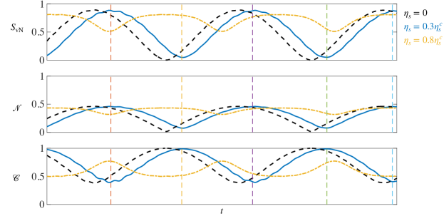
Figure 9: Dynamics of (a) entanglement entropy, (b) negativity, and (c) concurrence for parameters as in Fig. 7 in the main text.

We can write down the atomic state as a superposition

$$|\psi\rangle=\alpha|0\rangle+\beta|1\rangle+\gamma|2\rangle+\delta|3\rangle,$$ (40)

where $\alpha=\langle c_{0}\rangle,$ $\beta=\langle c_{1}\rangle,$ $\gamma=\langle c_{2}\rangle$ and $\delta=\langle c_{3}\rangle,$ with $|\alpha|^{2}+|\beta|^{2}+|\gamma|^{2}+|\delta|^{2}=1$ as the total number of atoms is conserved and normalized. Rewriting states $\ket{0},\ldots,\ket{3}$ in terms of spin and momentum states, see Eq. (1), the state of the system reads

$$|\psi\rangle=\alpha|0\rangle_{m}\otimes|\downarrow\rangle_{s}+\beta|1\rangle_{m}\otimes|\downarrow\rangle_{s}+\gamma|0\rangle_{m}\otimes|\uparrow\rangle_{s}+\delta|1\rangle_{m}\otimes|\uparrow\rangle_{s}.$$ (41)

We now can construct a reduced density matrix by summing over the spin degree of freedom

$$\tilde{\rho}=\langle\mbox{spin}|\psi\rangle\langle\psi|\mbox{spin}\rangle$$ (42)

or by summing over the momentum states

$$\tilde{\rho}=\langle\mbox{momentum}|\psi\rangle\langle\psi|\mbox{momentum}\rangle.$$ (43)

The reduced density matrix reads

$$\tilde{\rho}=\left[\begin{array}[]{ll}|\alpha|^{2}+|\beta|^{2}&\alpha\gamma^{*}+\beta\delta^{*}\\ \alpha^{*}\gamma+\beta^{*}\delta&|\gamma|^{2}+|\delta|^{2}\end{array}\right]$$ (44)

and can be easily diagonalized. The eigenvalues of this reduced density matrix are

$$\lambda=\dfrac{1}{2}\pm\dfrac{1}{2}\sqrt{1-4\left(|\alpha|^{2}|\delta|^{2}+|\beta|^{2}|\gamma|^{2}-\alpha\beta^{*}\gamma^{*}\delta-\alpha^{*}\beta\gamma\delta^{*}\right)}$$

or can alternatively be rewritten in terms of spins

$$\lambda=\dfrac{1}{2}\pm\dfrac{1}{2}\sqrt{1-4\left(S_{03}^{-}S_{03}^{+}+S_{12}^{-}S_{12}^{+}-J_{01}^{+}J_{23}^{-}-J_{01}^{-}J_{23}^{+}\right)}.$$

When $\eta=0,$ the system always remains in the pure state as the momentum state is separable in this case; in the superradiant phase, the fraction of atoms in the excited momentum state for $m_{F}=0$ is the same as the fraction of excited states for $m_{F}=1$.

On the other hand, when $\eta_{s}=0,$ the interaction $\eta$ induces entanglement between spin and momentum. The easiest way to see this is to consider the two-level case when all atoms are initially prepared in state $\ket{0}.$ Then, by increasing the coupling $\eta$ above its critical value, the wave function of the state becomes $\psi=\alpha\ket{0}+\delta\ket{3}=\alpha|0\rangle_{m}\otimes|\downarrow\rangle_{s}+\delta|1\rangle_{m}\otimes|\uparrow\rangle_{s},$ which is not separable in spin and momentum and, thus, is entangled. This state is maximally entangled when $\alpha=\delta=1/\sqrt{2},$ and in terms of spin and momentum degrees of freedom, the state of the system is symmetric spin-momentum configuration.

Appendix F Spontaneous and explicit symmetry breaking

In this Appendix, we gather arguments to elucidate the source of the non-equilibrium oscillatory phases that arise when one coupling surpasses the critical threshold while the other remains below it [cf. red and blue regions in the phase diagram in Fig. 6(a)].

Let us consider the case when $\eta_{s}>\eta_{s}^{c},$ i.e., the cavity mode $a_{y}$ is the important mode. The SR transition in $H_{s}$ appears when the corresponding $\mathbb{Z}_{2}$ symmetry of the model is broken. For the subsystem built on the momentum states (via photon mode $a_{y}$, Baumann et al. (2010)), which is described by the Hamiltonian

$$H_{s}=\omega_{{y}}a_{{y}}^{\dagger}a_{{y}}+\omega_{0}\left({c}_{1}^{\dagger}{c}_{1}+{c}_{3}^{\dagger}{c}_{3}\right)+\eta_{s}\left({a}_{{y}}+{a}_{{y}}^{\dagger}\right)\left({c}_{0}^{\dagger}{c}_{1}+{c}_{1}^{\dagger}{c}_{0}+{c}_{2}^{\dagger}{c}_{3}+{c}_{3}^{\dagger}{c}_{2}\right),$$ (45)

we have the condition

$$a_{y} \to-a_{y}$$ (46)

$$\left({c}_{0}^{\dagger}{c}_{1}+{c}_{1}^{\dagger}{c}_{0}+{c}_{2}^{\dagger}{c}_{3}+{c}_{3}^{\dagger}{c}_{2}\right) \to-\left({c}_{0}^{\dagger}{c}_{1}+{c}_{1}^{\dagger}{c}_{0}+{c}_{2}^{\dagger}{c}_{3}+{c}_{3}^{\dagger}{c}_{2}\right).$$

The second line above corresponds to $J^{x}\to-J^{x}$ for the Dicke model. Under the corresponding transformation in Eq. (12) the bosonic part of the Hamiltonian transforms as

$$\left({c}_{0}^{\dagger}{c}_{1}+{c}_{1}^{\dagger}{c}_{0}+{c}_{2}^{\dagger}{c}_{3}+{c}_{3}^{\dagger}{c}_{2}\right)\to\left({c}_{0}^{\dagger}{c}_{1}e^{i\left(\phi_{0}-\phi_{1}\right)}+{c}_{1}^{\dagger}{c}_{0}e^{i\left(\phi_{1}-\phi_{0}\right)}+{c}_{2}^{\dagger}{c}_{3}e^{i\left(\phi_{2}-\phi_{3}\right)}+{c}_{3}^{\dagger}{c}_{2}e^{i\left(\phi_{3}-\phi_{2}\right)}\right)$$ (47)

$$=-\left({c}_{0}^{\dagger}{c}_{1}+{c}_{1}^{\dagger}{c}_{0}+{c}_{2}^{\dagger}{c}_{3}+{c}_{3}^{\dagger}{c}_{2}\right),$$

thus seting the constrains $e^{\pm i\left(\phi_{1}-\phi_{0}\right)}=-1$ and $e^{\pm i\left(\phi_{2}-\phi_{3}\right)}=-1$. These constraints bring us to the following condition on the relative phases:

$$\phi_{0}-\phi_{1} =\pi\pm 2\pi n$$ (48)

$$\phi_{2}-\phi_{3} =\pi\pm 2\pi m.$$

As only the relative phase between two bosonic fields enters the Hamiltonian, we get two conditions for four phases. If we perform the same transformation on the second interacting term in the Hamiltonian

$$\eta\left({a}_{z}+{a}_{z}^{\dagger}\right)\left({c}_{1}^{\dagger}{c}_{2}+{c}_{0}^{\dagger}{c}_{3}+{c}_{2}^{\dagger}{c}_{1}+{c}_{3}^{\dagger}{c}_{0}\right),$$ (49)

we find that it induces an additional phase for photon field $a_{z},$ which provokes an explicit symmetry breaking

$$\eta\left({a}_{{z}}e^{-i\phi_{z}}+{a}_{{z}}^{\dagger}e^{i\phi_{z}}\right)\left({c}_{1}^{\dagger}{c}_{2}e^{i\left(\phi_{1}-\phi_{2}\right)}+{c}_{0}^{\dagger}{c}_{3}e^{i\left(\phi_{0}-\phi_{3}\right)}+{c}_{2}^{\dagger}{c}_{1}e^{-i\left(\phi_{1}-\phi_{2}\right)}+{c}_{3}^{\dagger}{c}_{0}e^{-i\left(\phi_{0}-\phi_{3}\right)}\right)=$$ (50)

$$=\eta\left({a}_{{z}}e^{-i\phi_{z}}+{a}_{{z}}^{\dagger}e^{i\phi_{z}}\right)\left({c}_{1}^{\dagger}{c}_{2}e^{i\left(\phi_{1}-\phi_{3}-\pi\right)}+{c}_{0}^{\dagger}{c}_{3}e^{i\left(\phi_{1}+\pi-\phi_{3}\right)}+{c}_{2}^{\dagger}{c}_{1}e^{-i\left(\phi_{1}-\phi_{3}-\pi\right)}+{c}_{3}^{\dagger}{c}_{0}e^{-i\left(\phi_{1}+\pi-\phi_{3}\right)}\right)=$$

$$=-\eta\left({a}_{{z}}e^{-i\phi_{z}}+{a}_{{z}}^{\dagger}e^{i\phi_{z}}\right)\left({c}_{1}^{\dagger}{c}_{2}e^{i\left(\phi_{1}-\phi_{3}\right)}+{c}_{0}^{\dagger}{c}_{3}e^{i\left(\phi_{1}-\phi_{3}\right)}+{c}_{2}^{\dagger}{c}_{1}e^{-i\left(\phi_{1}-\phi_{3}\right)}+{c}_{3}^{\dagger}{c}_{0}e^{-i\left(\phi_{1}-\phi_{3}\right)}\right).$$

One can recognize that the bosonic part gains a phase $\pm\left(\phi_{1}-\phi_{3}\right)$ which, generally, can take an arbitrary value. So, as soon as we turn on coupling $\eta$, we break the symmetry of the Hamiltonian. In general, to restore the symmetry at finite time $T$, the population of a corresponding atomic level must decay to zero.

The breaking of the symmetry can be seen also in the following calculation. Given the steady state for $\eta_{s}>\eta_{s}^{c}$ and $\eta=0$ [cf. Eq. (37)], after quenching $\eta$, the photon mode $a_{z}$ becomes

$$a_{z}=-2\dfrac{\eta\left(\omega_{z}-i\kappa\right)}{\left(\omega_{z}^{2}+\kappa^{2}\right)}\left(\sqrt{(1-\mu)\mu(1+2J^{z})\left(1-2J^{z}\right)}\right)$$ (51)

which is non-zero for $\mu\neq 0,1$. Here, the typical time at which the photon approaches the value above is $\approx\text{1/$\kappa$}$ negligibly small. The explicit breaking of the symmetry in the term

$$\eta\left({a}_{z}+{a}_{z}^{\dagger}\right)\left({c}_{1}^{\dagger}{c}_{2}+{c}_{0}^{\dagger}{c}_{3}+{c}_{2}^{\dagger}{c}_{1}+{c}_{3}^{\dagger}{c}_{0}\right)\to$$ (52)

$$-\eta\left({a}_{{z}}e^{-i\phi_{z}}+{a}_{{z}}^{\dagger}e^{i\phi_{z}}\right)\left({c}_{1}^{\dagger}{c}_{2}e^{i\left(\phi_{1}-\phi_{3}\right)}+{c}_{0}^{\dagger}{c}_{3}e^{i\left(\phi_{1}-\phi_{3}\right)}+{c}_{2}^{\dagger}{c}_{1}e^{-i\left(\phi_{1}-\phi_{3}\right)}+{c}_{3}^{\dagger}{c}_{0}e^{-i\left(\phi_{1}-\phi_{3}\right)}\right)$$

takes the system out of equilibrium. To equilibrate the system, the Hamiltonian must regain the symmetry via one of two mechanisms:

1. The decay of the photon number of the auxiliary mode to zero.

2. The phases of the bosons adjusting to satisfy the condition $\phi_{1}-\phi_{3}\equiv 0.$

The oscillatory phase accompanies the system’s dynamics until one of these two possibilities is realized. Below, we discuss both scenarios in more detail.

Appendix G Relaxation dynamics at late times

In this Appendix, we study the properties of the system at late times and evaluate the time $T$ at which the system restores its symmetry.

To restore the explicitly broken symmetry one needs to tune the emergent phases in front of the auxiliary photons, $\phi_{c}$, and pseudo-spins, $\phi_{i}-\phi_{j}$, to zero. This procedure can be trivially done when the corresponding occupation of the photon or atomic levels equals zero due to the ambiguity of the phase of these complex numbers when their magnitude is zero. In the former case, the symmetry restoration occurs asymptotically at time $T\to\infty$ through the slow decay of the cavity photon magnitude induced by the dissipation $\kappa$. In line with this scenario, the dynamics, when expressed in terms of the two cavity fields, resemble the behavior depicted in the middle panels of Fig. 6(c-d) during the course of the experiment.

According to the second mechanism, which takes a finite time $T$, during dynamics all particles slowly transfer to the lowest energy pair of ground and excited momentum states. For instance, if $\omega_{s}>0,$ all particles will redistribute to levels $\ket{0}$ and $\ket{1}$ resulting into $\left\langle c_{2}(T)\right\rangle=0$ and $\left\langle c_{3}(T)\right\rangle=0$. Then, when states with higher energy become empty, the explicitly broken symmetry of the system can be restored. Eventually, the phases of both cavity fields remain constant, and both fields start approaching true superradiant states with $n_{y}\neq 0$ and $n_{z}\neq 0$, cf. the right panels in Fig. 6(c-d).

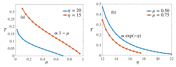
Figure 10: Symmetry restoration time $T$ (in seconds) as a function of (a) the initial population of the level $\ket{0}$, i.e., $N_{0}=\mu N$ and (b) of the photon-matter coupling to the auxiliary cavity field. Here we consider mode $a_{y}$ as the main and mode $a_{z}$ as the auxiliary.

Fig. 10 shows the scaling of the relaxation time with (a) the fraction of particles at $t=0$ in state $\ket{0},$ and (b) with the strength of the smaller of the two couplings, i.e, auxiliary one. Here we consider the mode $a_{z}$ as the auxiliary one for simplicity since its critical coupling does not depend on $\mu$. The finite time $T$ corresponds to the scenario when symmetry restoration takes place through the transferring of all particles to the lower energy pair of ground and excited momentum states. For instance, for $\omega_{s}>0$, the more particles are initially prepared in state $\ket{2},$ the longer is $T$ [cf. Fig. 10(a)]. Assuming that the speed of particles transferring from levels $\ket{2}$ and $\ket{3}$ remains constant and depends solely on the couplings and detunings, the relaxation time will be proportional to the population of the zero momentum state with the higher energy. One would estimate in this case $T\propto(1-\mu)$ as we confirm numerically in panel (a). At the same time, when $\omega_{s}<0,$ the pair of states that have smaller energy are $\ket{2}$ and $\ket{1},$ and the relaxation time scales like $T\propto\mu.$ This can also be seen from the Hamiltonian $H_{\operatorname{tot}}$ which in the normal state is invariant under the transformation $\mu\leftrightarrow 1-\mu$ when $\omega_{s}\to-\omega_{s}.$

On the other hand, the symmetry restoration time scales with the coupling to the auxiliary mode [$\eta$ in Fig. 10(b)] like $T\propto\exp(-\eta).$ It means that the closer this auxiliary coupling is to its critical value, the faster the symmetry is restored. Consequently, operating within a parameter regime where the coupling to the auxiliary mode remains significantly below the critical threshold, yet remains finite, gives us the opportunity to probe the atomic dynamics within the system with minimal disruption.

Below we consider a few fine-tuned limits in which a stationary state can not be reached within the operational timescales of the experiment.

G.1 $\kappa/\omega_{c}\to\infty$ limit

The relaxation time $T$ depends on the strength of the photon-matter coupling with the auxiliary mode; namely, the stronger the interaction, the faster the relaxation [see Fig. 10(b)]. On the other hand, the strength of this coupling controls the population of the auxiliary cavity mode, $n\propto\eta^{2}/(\omega_{c}^{2}+\kappa^{2}).$ As such, it is instructive to explore the regime where $\eta/\sqrt{\omega_{c}^{2}+\kappa^{2}}$ is large enough to produce sufficiently large cavity field amplitude to enable detections of oscillations in the auxiliary cavity field. We would also like to simultaneously satisfy the condition $\eta\ll\eta_{c}$ so that the system’s restoration of its symmetry becomes protracted to exponentially late times. These conditions can be satisfied simultaneously when $\omega_{c}\ll\kappa$, a regime in which the critical coupling diverges like $\sqrt{\omega_{0}\kappa^{2}/\omega_{c}}$. The extreme case of $\omega_{c}=0$ corresponds to the critical coupling tending to infinity. Counter-intuitively, in this case, one enters a strong dissipation regime which prevents the relaxation.

The main idea of why the strong dissipation regime prevents relaxation can be explained as follows: according to the Hamiltonian $H_{\operatorname{tot}}$ [Eq. (8)], pseudo-spins are coupled to the real quadrature of the cavity fields, $a+a^{\dagger}$. If the cavity fields are coupled to the $x-$components of pseudo-spins, then the cavity field is imaginary, $a_{y}\propto 2J^{x}/(-i\kappa)$ (or $a_{z}\propto 2S^{x}/(-i\kappa)$). Here the cavity decay rate causes a phase shift $\phi_{\kappa}^{y,z}=\tan^{-1}\left(-\kappa/\omega_{y,z}\right)$ of the field scattered into the cavity by the atomic system Dogra et al. (2019). Thus, by setting the cavity detuning $\omega_{y}$ or $\omega_{z}$ to be much smaller than $\kappa$, one can make the corresponding cavity field imaginary and eliminate its feedback on the spin dynamics. For instance, when $\eta_{s}>\eta_{s}^{c},$ $\eta<\eta^{c}$ and $\omega_{y}\neq 0,$ $\omega_{z}\to 0$ [blue region in Fig. 6(a)], $a_{y}$ approaches its steady state value, while $a_{z}\approx-2\eta\left(S_{03}^{x}+S_{12}^{x}\right)/\left(-i\kappa\right)$ oscillates together with the precession of the pseudo-spin $S^{x}.$ However, as $(a_{z}+a_{z}^{\dagger})\to 0,$ the non-stationary behavior of the cavity field does not impact the dynamics of pseudo-spin $S^{x}$. In other words, subsystem $H_{s}$ constantly induces precession for pseudo-spin $S^{x}$ (and thus oscillations to the cavity mode $a_{z}$) due to the explicit symmetry breaking; it does not, however, experience feedback from subsystem $H.$ As a result, the lack of reciprocal interaction between the two subsystems prevents the system from reaching a steady state, and oscillations in the auxiliary cavity mode $a_{z}$ survive for an arbitrarily long time.

When $\eta_{s}<\eta_{s}^{c}$ and $\eta>\eta^{c}$ [red region in the phase diagram in Fig. 6(a)], one should set $\omega_{y}\ll\kappa$ to prevent the system from reaching its steady state. In this case, the cavity mode $a_{y}$ will exhibit oscillations around zero for an arbitrarily long time, reflecting the precession of pseudo-spin $J^{x}$. The cavity mode $a_{z}$, in turn, will approach its steady state value, determined solely by the Hamiltonian $H$ [Eq. (2)] and initial conditions.

Interestingly, in the opposite limit where $\omega_{c}\gg\kappa$, the system can also experience slow relaxation. The critical coupling scales like $\eta_{c}\propto\sqrt{\omega_{0}\omega_{c}}\to\infty$; it is easier to keep the coupling strongly subcritical while still large enough to enable read-out. However, as the cavity occupation scales as $n\propto 1/\omega_{c}^{2}$, in order to keep $n$ non-zero, it is essential to keep the cavity detuning finite.

G.2 $\omega_{s}\to 0$ limit

One can recognize from the level scheme in Fig. 2(b) that when $\omega_{s}=0,$ the two ground states in the momentum variables, $\ket{0},\ket{2}$, and the two excited ones $\ket{1},\ket{3}$ are degenerate. In this case, the Hamiltonian acquires an additional symmetry under exchange between ground or excited states, namely $c_{1}\leftrightarrow c_{3},$ $c_{0}\leftrightarrow c_{2}$ (see Hamiltonian in the bosonic representation in Appendix A). As a consequence, the dynamics for the pair of fields $c_{1},c_{3}$ (and likewise for $c_{0},c_{2}$) occur at the same frequencies $c_{1},c_{3}\propto\exp(i\Omega t).$ Accordingly, the phase that explicitly breaks the symmetry of the Hamiltonian, $\pm(\phi_{1}-\phi_{3}),$ remains constant over time, determined solely by the initial conditions (which can be arbitrary and are not restricted in general). Thus, after the quench, both spins $J^{x}$ and $S^{x}$ gain fixed time values, and one can observe superradiance in both cavity modes simultaneously. Interestingly, in this case, $n_{y}$ and $n_{z}$ do not oscillate over time, and non-stationary behavior can only be observed at the level of the atomic observables. In particular, particles redistribute between different excited or ground momentum states so that the overall number of particles in the upper and lower spinor components oscillates over time around a common time-averaged value.

Appendix H Three-level model

We now revisit the possibility of probing the system’s dynamics with the auxiliary cavity field in a three-level system. As mentioned in the main text, such a model includes single ground momentum state $\ket{2}$, and two excited momentum states $\ket{1},$ $\ket{3},$ where we keep notation as in the Eq. (1). Such Hamiltonian can be implemented when fixing $\mathbf{e}_{p}=\mathbf{e}_{x}$ in Eq. (20) and considering resonant spin changing and spin-dependent processes, cf. implementations in Refs. Dogra et al. (2019); Ferri et al. (2021). Here we omit the implementation of the three-level model, concentrating mostly on the physical phenomena, compared to the four-level model in Eq. (8). To do so, we study the effect of spontaneous symmetry breaking in one sector of the Hamiltonian on the dynamical properties in another sector. As we demonstrate below, explicit symmetry breaking in the self-ordered phase(s) is not pronounced in the three-level case, thereby resulting in trivial system dynamics.

The Hamiltonian of our three-level model reads

$$H_{3} =\omega_{{y}}a_{{y}}^{\dagger}a_{{y}}+\omega_{{z}}a_{{z}}^{\dagger}a_{{z}}+\omega_{0}\left({c}_{1}^{\dagger}{c}_{1}+{c}_{3}^{\dagger}{c}_{3}\right)+\omega_{s}({c}_{2}^{\dagger}{c}_{2}+{c}_{3}^{\dagger}{c}_{3})+$$ (53)

$$+\eta\left({a}_{{z}}+{a}_{{z}}^{\dagger}\right)\left({c}_{1}^{\dagger}{c}_{2}+{c}_{2}^{\dagger}{c}_{1}\right)+\eta_{s}\left({a}_{{y}}+{a}_{{y}}^{\dagger}\right)\left({c}_{2}^{\dagger}{c}_{3}+{c}_{3}^{\dagger}{c}_{2}\right).$$

Let us consider the effect of the spontaneous symmetry breaking in one subsystem on the dynamics of another, similarly as it is done in Appendix F. Firstly, we consider a steady state when $\eta_{s}>\eta_{s}^{c}$ and $\eta=0$. In this case, the symmetry of a subsystem involving photon mode $a_{y}$ is broken, meaning there exist two solutions, satisfying

$$a_{y} \rightarrow-a_{y}$$ (54)

$$\left({c}_{2}^{\dagger}{c}_{3}+{c}_{3}^{\dagger}{c}_{2}\right) \rightarrow-\left({c}_{2}^{\dagger}{c}_{3}+{c}_{3}^{\dagger}{c}_{2}\right).$$

Applying transformation (12), we can see that such transformation

$$\left({c}_{2}^{\dagger}{c}_{3}+{c}_{3}^{\dagger}{c}_{2}\right) \to\left({c}_{2}^{\dagger}{c}_{3}e^{i\left(\phi_{2}-\phi_{3}\right)}+{c}_{3}^{\dagger}{c}_{2}e^{i\left(\phi_{3}-\phi_{2}\right)}\right)$$ (55)

$$=-\left({c}_{2}^{\dagger}{c}_{3}+{c}_{3}^{\dagger}{c}_{2}\right)$$

sets the following constraints on relative phases

$$\phi_{2}-\phi_{3}=\pi\pm 2\pi m.$$ (56)

Note that there are no restrictions on the phase $\phi_{1}$ because photon mode $a_{y}$ is not coupled to the level $\ket{1}$. As such, making the second coupling, $\eta$, non-zero does not induce explicit symmetry breaking. This fact can be seen by applying the transformation (12) to this term:

$$\left({a}_{{z}}e^{-i\phi_{z}}+{a}_{{z}}^{\dagger}e^{i\phi_{z}}\right)\left({c}_{1}^{\dagger}{c}_{2}e^{i\left(\phi_{1}-\phi_{2}\right)}+{c}_{2}^{\dagger}{c}_{1}e^{-i\left(\phi_{1}-\phi_{2}\right)}\right)\propto\langle c_{1}\rangle\equiv 0.$$ (57)

The phase of the boson field $c_{1}$ can always compensate for the restricted phase of $c_{2}$. Note that we assume that level $\ket{1}$ is unoccupied before increasing $\eta$, and thus the phase of $c_{1}$ can be changed arbitrarily. The system is therefore stable against quenches $\eta<\eta^{c}$. This behavior arises from the fact that each photon mode is not coupled to all atomic levels; symmetry breaking in one interaction term does not imply explicit symmetry breaking in another. More precisely, when $\eta_{s}>\eta_{s}^{c}$ and $\eta=0$, one finds that

$$c_{1}^{\dagger}c_{1} =0$$ (58)

$$c_{2}^{\dagger}c_{2} =\frac{\left(1-2J^{z}\right)}{2}$$

$$c_{3}^{\dagger}c_{3} =\frac{\left(1+2J_{z}\right)}{2}$$

and after the quench of $\eta$, we get $a_{z}\propto\left(c_{1}^{\dagger}c_{2}+c_{2}^{\dagger}c_{1}\right)=0$ and the subsystem remains in steady state as long as $\eta/\eta^{c}<\eta_{s}/\eta_{s}^{c}$. The absence of restrictions on phase $\phi_{1}$ makes it impossible to induce competing conditions and push the subsystem out of equilibrium. Indeed, in the case of four levels, one cannot manipulate the phase of a single boson separately, thereby resulting in the existence of long-lived oscillations of the auxiliary cavity field and the precession of corresponding pseudo-spins.

References

- Sakurai and Commins (1995) Jun John Sakurai and Eugene D Commins, “Modern quantum mechanics, revised edition,” (1995).
- Hirsch (1999) J. E. Hirsch, “Spin hall effect,” Phys. Rev. Lett. 83, 1834–1837 (1999).
- Hasan and Kane (2010) M. Z. Hasan and C. L. Kane, “Colloquium: Topological insulators,” Rev. Mod. Phys. 82, 3045–3067 (2010).
- Sato and Ando (2017) Masatoshi Sato and Yoichi Ando, “Topological superconductors: a review,” Reports on Progress in Physics 80, 076501 (2017).
- Sau et al. (2010) Jay D. Sau, Roman M. Lutchyn, Sumanta Tewari, and S. Das Sarma, “Generic new platform for topological quantum computation using semiconductor heterostructures,” Phys. Rev. Lett. 104, 040502 (2010).
- Qi et al. (2023a) Jiaan Qi, Zhi-Hai Liu, and HQ Xu, “Spin-orbit interaction enabled high-fidelity two-qubit gates,” arXiv preprint arXiv:2308.06986 (2023a).
- Stav et al. (2018) Tomer Stav, Arkady Faerman, Elhanan Maguid, Dikla Oren, Vladimir Kleiner, Erez Hasman, and Mordechai Segev, “Quantum entanglement of the spin and orbital angular momentum of photons using metamaterials,” Science 361, 1101–1104 (2018), https://www.science.org/doi/pdf/10.1126/science.aat9042 .
- Kale et al. (2020) Sumit Suresh Kale, Yijue Ding, Yong P Chen, Bretislav Friedrich, and Sabre Kais, “Spin-momentum entanglement in a bose–einstein condensate,” Physical Chemistry Chemical Physics 22, 25669–25674 (2020).
- Manzoni et al. (2017) Marco T Manzoni, Ludwig Mathey, and Darrick E Chang, “Designing exotic many-body states of atomic spin and motion in photonic crystals,” Nature communications 8, 14696 (2017).
- Mivehvar et al. (2021) Farokh Mivehvar, Francesco Piazza, Tobias Donner, and Helmut Ritsch, “Cavity qed with quantum gases: new paradigms in many-body physics,” Advances in Physics 70, 1–153 (2021).
- Dogra et al. (2019) Nishant Dogra, Manuele Landini, Katrin Kroeger, Lorenz Hruby, Tobias Donner, and Tilman Esslinger, “Dissipation-induced structural instability and chiral dynamics in a quantum gas,” Science 366, 1496–1499 (2019).
- Baumann et al. (2010) Kristian Baumann, Christine Guerlin, Ferdinand Brennecke, and Tilman Esslinger, “Dicke quantum phase transition with a superfluid gas in an optical cavity,” nature 464, 1301–1306 (2010).
- Kroeze et al. (2019) Ronen M. Kroeze, Yudan Guo, and Benjamin L. Lev, “Dynamical spin-orbit coupling of a quantum gas,” Phys. Rev. Lett. 123, 160404 (2019).
- Marino et al. (2022) Jamir Marino, Martin Eckstein, Matthew Foster, and Ana-Maria Rey, “Dynamical phase transitions in the collisionless pre-thermal statesof isolated quantum systems: theory and experiments,” Reports on Progress in Physics (2022).
- Klinder et al. (2015) Jens Klinder, Hans Keßler, Matthias Wolke, Ludwig Mathey, and Andreas Hemmerich, “Dynamical phase transition in the open dicke model,” Proceedings of the National Academy of Sciences 112, 3290–3295 (2015), https://www.pnas.org/doi/pdf/10.1073/pnas.1417132112 .
- Skulte et al. (2021) Jim Skulte, Phatthamon Kongkhambut, Hans Keßler, Andreas Hemmerich, Ludwig Mathey, and Jayson G. Cosme, “Parametrically driven dissipative three-level dicke model,” Phys. Rev. A 104, 063705 (2021).
- Kongkhambut et al. (2021) Phatthamon Kongkhambut, Hans Keßler, Jim Skulte, Ludwig Mathey, Jayson G. Cosme, and Andreas Hemmerich, “Realization of a periodically driven open three-level dicke model,” Phys. Rev. Lett. 127, 253601 (2021).
- Kongkhambut et al. (2022) Phatthamon Kongkhambut, Jim Skulte, Ludwig Mathey, Jayson G. Cosme, Andreas Hemmerich, and Hans Keßler, “Observation of a continuous time crystal,” Science 377, 670–673 (2022), https://www.science.org/doi/pdf/10.1126/science.abo3382 .
- Lewis-Swan et al. (2021) Robert J. Lewis-Swan, Diego Barberena, Julia R. K. Cline, Dylan J. Young, James K. Thompson, and Ana Maria Rey, “Cavity-qed quantum simulator of dynamical phases of a bardeen-cooper-schrieffer superconductor,” Phys. Rev. Lett. 126, 173601 (2021).
- Carollo and Lesanovsky (2021) Federico Carollo and Igor Lesanovsky, “Exactness of mean-field equations for open dicke models with an application to pattern retrieval dynamics,” Phys. Rev. Lett. 126, 230601 (2021).
- Seetharam et al. (2022a) K. Seetharam, A. Lerose, R. Fazio, and J. Marino, “Correlation engineering via nonlocal dissipation,” Phys. Rev. Res. 4, 013089 (2022a).
- Seetharam et al. (2022b) K. Seetharam, A. Lerose, R. Fazio, and J. Marino, “Dynamical scaling of correlations generated by short- and long-range dissipation,” Phys. Rev. B 105, 184305 (2022b).
- Marino (2022) Jamir Marino, “Universality class of ising critical states with long-range losses,” Phys. Rev. Lett. 129, 050603 (2022).
- Periwal et al. (2021) Avikar Periwal, Eric S Cooper, Philipp Kunkel, Julian F Wienand, Emily J Davis, and Monika Schleier-Smith, “Programmable interactions and emergent geometry in an array of atom clouds,” Nature 600, 630–635 (2021).
- Finger et al. (2023) Fabian Finger, Rodrigo Rosa-Medina, Nicola Reiter, Panagiotis Christodoulou, Tobias Donner, and Tilman Esslinger, “Spin- and momentum-correlated atom pairs mediated by photon exchange,” (2023), arXiv:2303.11326 [cond-mat.quant-gas] .
- Rosa-Medina et al. (2022) Rodrigo Rosa-Medina, Francesco Ferri, Fabian Finger, Nishant Dogra, Katrin Kroeger, Rui Lin, R. Chitra, Tobias Donner, and Tilman Esslinger, “Observing dynamical currents in a non-hermitian momentum lattice,” Phys. Rev. Lett. 128, 143602 (2022).
- Lin et al. (2022) Rui Lin, Rodrigo Rosa-Medina, Francesco Ferri, Fabian Finger, Katrin Kroeger, Tobias Donner, Tilman Esslinger, and R. Chitra, “Dissipation-engineered family of nearly dark states in many-body cavity-atom systems,” Phys. Rev. Lett. 128, 153601 (2022).
- Skulte et al. (2023) Jim Skulte, Phatthamon Kongkhambut, Sahana Rao, Ludwig Mathey, Hans Keßler, Andreas Hemmerich, and Jayson G. Cosme, “Condensate formation in a dark state of a driven atom-cavity system,” Phys. Rev. Lett. 130, 163603 (2023).
- Piñeiro Orioli et al. (2022) A. Piñeiro Orioli, J. K. Thompson, and A. M. Rey, “Emergent dark states from superradiant dynamics in multilevel atoms in a cavity,” Phys. Rev. X 12, 011054 (2022).
- Soriente et al. (2018) M. Soriente, T. Donner, R. Chitra, and O. Zilberberg, “Dissipation-induced anomalous multicritical phenomena,” Phys. Rev. Lett. 120, 183603 (2018).
- Landini et al. (2018) Manuele Landini, Nishant Dogra, Katrin Kröger, Lorenz Hruby, Tobias Donner, and Tilman Esslinger, “Formation of a spin texture in a quantum gas coupled to a cavity,” Physical review letters 120, 223602 (2018).
- Dreon et al. (2022) Davide Dreon, Alexander Baumgärtner, Xiangliang Li, Simon Hertlein, Tilman Esslinger, and Tobias Donner, “Self-oscillating pump in a topological dissipative atom–cavity system,” Nature 608, 494–498 (2022).
- Nagy et al. (2010) D. Nagy, G. Kónya, G. Szirmai, and P. Domokos, “Dicke-model phase transition in the quantum motion of a bose-einstein condensate in an optical cavity,” Phys. Rev. Lett. 104, 130401 (2010).
- Zhiqiang et al. (2017) Zhang Zhiqiang, Chern Hui Lee, Ravi Kumar, KJ Arnold, Stuart J Masson, AS Parkins, and MD Barrett, “Nonequilibrium phase transition in a spin-1 dicke model,” Optica 4, 424–429 (2017).
- Masson et al. (2017) Stuart J. Masson, M. D. Barrett, and Scott Parkins, “Cavity qed engineering of spin dynamics and squeezing in a spinor gas,” Phys. Rev. Lett. 119, 213601 (2017).
- Ferri et al. (2021) Francesco Ferri, Rodrigo Rosa-Medina, Fabian Finger, Nishant Dogra, Matteo Soriente, Oded Zilberberg, Tobias Donner, and Tilman Esslinger, “Emerging dissipative phases in a superradiant quantum gas with tunable decay,” Phys. Rev. X 11, 041046 (2021).
- Kroeze et al. (2018) Ronen M. Kroeze, Yudan Guo, Varun D. Vaidya, Jonathan Keeling, and Benjamin L. Lev, “Spinor self-ordering of a quantum gas in a cavity,” Phys. Rev. Lett. 121, 163601 (2018).
- Mivehvar et al. (2017) Farokh Mivehvar, Francesco Piazza, and Helmut Ritsch, “Disorder-driven density and spin self-ordering of a bose-einstein condensate in a cavity,” Phys. Rev. Lett. 119, 063602 (2017).
- Wilson et al. (2022) John Drew Wilson, Simon B. Jäger, Jarrod T. Reilly, Athreya Shankar, Maria Luisa Chiofalo, and Murray J. Holland, “Beyond one-axis twisting: Simultaneous spin-momentum squeezing,” Phys. Rev. A 106, 043711 (2022).
- Nagy et al. (2011) D. Nagy, G. Szirmai, and P. Domokos, “Critical exponent of a quantum-noise-driven phase transition: The open-system dicke model,” Phys. Rev. A 84, 043637 (2011).
- Stitely et al. (2022) Kevin C. Stitely, Andrus Giraldo, Bernd Krauskopf, and Scott Parkins, “Lasing and counter-lasing phase transitions in a cavity-qed system,” Phys. Rev. Res. 4, 023101 (2022).
- Lerose and Pappalardi (2020) Alessio Lerose and Silvia Pappalardi, “Bridging entanglement dynamics and chaos in semiclassical systems,” Phys. Rev. A 102, 032404 (2020).
- Defenu et al. (2023) Nicolò Defenu, Alessio Lerose, and Silvia Pappalardi, “Out-of-equilibrium dynamics of quantum many-body systems with long-range interactions,” (2023), arXiv:2307.04802 [cond-mat.quant-gas] .
- Kirton et al. (2019) Peter Kirton, Mor M Roses, Jonathan Keeling, and Emanuele G Dalla Torre, “Introduction to the dicke model: From equilibrium to nonequilibrium, and vice versa,” Advanced Quantum Technologies 2, 1800043 (2019).
- Nielsen and Chuang (2010) Michael A. Nielsen and Isaac L. Chuang, Quantum Computation and Quantum Information: 10th Anniversary Edition (Cambridge University Press, 2010).
- Zhang et al. (2018) Zhiqiang Zhang, Chern Hui Lee, Ravi Kumar, K. J. Arnold, Stuart J. Masson, A. L. Grimsmo, A. S. Parkins, and M. D. Barrett, “Dicke-model simulation via cavity-assisted raman transitions,” Phys. Rev. A 97, 043858 (2018).
- Chelpanova et al. (2023) Oksana Chelpanova, Alessio Lerose, Shu Zhang, Iacopo Carusotto, Yaroslav Tserkovnyak, and Jamir Marino, “Intertwining of lasing and superradiance under spintronic pumping,” Phys. Rev. B 108, 104302 (2023).
- Dicke (1954) R. H. Dicke, “Coherence in spontaneous radiation processes,” Phys. Rev. 93, 99–110 (1954).
- Dimer et al. (2007) F. Dimer, B. Estienne, A. S. Parkins, and H. J. Carmichael, “Proposed realization of the dicke-model quantum phase transition in an optical cavity qed system,” Phys. Rev. A 75, 013804 (2007).
- Kirton and Keeling (2018) Peter Kirton and Jonathan Keeling, “Superradiant and lasing states in driven-dissipative dicke models,” New Journal of Physics 20, 015009 (2018).
- Mivehvar (2023) Farokh Mivehvar, “Unconventional dicke model: Multistabilities and nonequilibrium dynamics,” (2023), arXiv:2307.05686 [quant-ph] .
- Marsh et al. (2023) Brendan P Marsh, Ronen M Kroeze, Surya Ganguli, Sarang Gopalakrishnan, Jonathan Keeling, and Benjamin L Lev, “Entanglement and replica symmetry breaking in a driven-dissipative quantum spin glass,” arXiv preprint arXiv:2307.10176 (2023).
- Cornfeld et al. (2018) Eyal Cornfeld, Moshe Goldstein, and Eran Sela, “Imbalance entanglement: Symmetry decomposition of negativity,” Phys. Rev. A 98, 032302 (2018).
- Wootters (2001) William K Wootters, “Entanglement of formation and concurrence.” Quantum Inf. Comput. 1, 27–44 (2001).
- Zou et al. (2022) Ji Zou, Shu Zhang, and Yaroslav Tserkovnyak, “Bell-state generation for spin qubits via dissipative coupling,” Physical Review B 106 (2022), 10.1103/physrevb.106.l180406.
- Vidal and Werner (2002) G. Vidal and R. F. Werner, “Computable measure of entanglement,” Phys. Rev. A 65, 032314 (2002).
- Huybrechts et al. (2020) Dolf Huybrechts, Fabrizio Minganti, Franco Nori, Michiel Wouters, and Nathan Shammah, “Validity of mean-field theory in a dissipative critical system: Liouvillian gap, -symmetric antigap, and permutational symmetry in the model,” Phys. Rev. B 101, 214302 (2020).
- Qi et al. (2023b) Zihao Qi, Thomas Scaffidi, and Xiangyu Cao, “Surprises in the deep hilbert space of all-to-all systems: From superexponential scrambling to slow entanglement growth,” Phys. Rev. B 108, 054301 (2023b).
- Iemini et al. (2023) Fernando Iemini, Darrick Chang, and Jamir Marino, “Dynamics of inhomogeneous spin ensembles with all-to-all interactions: breaking permutational invariance,” (2023), arXiv:2309.10746 [quant-ph] .
- Valencia-Tortora et al. (2023) Riccardo J. Valencia-Tortora, Shane P. Kelly, Tobias Donner, Giovanna Morigi, Rosario Fazio, and Jamir Marino, “Crafting the dynamical structure of synchronization by harnessing bosonic multilevel cavity qed,” Phys. Rev. Res. 5, 023112 (2023).
- Galitski and Spielman (2013) Victor Galitski and Ian B Spielman, “Spin–orbit coupling in quantum gases,” Nature 494, 49–54 (2013).
- Lorenzo et al. (2017) Salvatore Lorenzo, Jamir Marino, Francesco Plastina, G Massimo Palma, and Tony JG Apollaro, “Quantum critical scaling under periodic driving,” Scientific reports 7, 5672 (2017).
- Brennecke et al. (2013) Ferdinand Brennecke, Rafael Mottl, Kristian Baumann, Renate Landig, Tobias Donner, and Tilman Esslinger, “Real-time observation of fluctuations at the driven-dissipative dicke phase transition,” Proceedings of the National Academy of Sciences 110, 11763–11767 (2013), https://www.pnas.org/doi/pdf/10.1073/pnas.1306993110 .
- Bhaseen et al. (2012) M. J. Bhaseen, J. Mayoh, B. D. Simons, and J. Keeling, “Dynamics of nonequilibrium dicke models,” Phys. Rev. A 85, 013817 (2012).
- Damanet et al. (2019) Fran çois Damanet, Andrew J. Daley, and Jonathan Keeling, “Atom-only descriptions of the driven-dissipative dicke model,” Phys. Rev. A 99, 033845 (2019).
- Jäger et al. (2022) Simon B. Jäger, Tom Schmit, Giovanna Morigi, Murray J. Holland, and Ralf Betzholz, “Lindblad master equations for quantum systems coupled to dissipative bosonic modes,” Phys. Rev. Lett. 129, 063601 (2022).
- Keeling et al. (2010) J. Keeling, M. J. Bhaseen, and B. D. Simons, “Collective dynamics of bose-einstein condensates in optical cavities,” Phys. Rev. Lett. 105, 043001 (2010).
- Bhore et al. (2023) Tanmay Bhore, Jean-Yves Desaules, and Zlatko Papić, “Deep thermalization in constrained quantum systems,” (2023), arXiv:2307.03769 [quant-ph] .
- Valencia-Tortora et al. (2022) Riccardo J. Valencia-Tortora, Nicola Pancotti, and Jamir Marino, “Kinetically constrained quantum dynamics in superconducting circuits,” PRX Quantum 3, 020346 (2022).
- Orioli and Rey (2020) A Piñeiro Orioli and AM Rey, “Subradiance of multilevel fermionic atoms in arrays with filling ,” Physical Review A 101, 043816 (2020).
- Hotter et al. (2023) Christoph Hotter, Laurin Ostermann, and Helmut Ritsch, “Cavity sub- and superradiance for transversely driven atomic ensembles,” Phys. Rev. Res. 5, 013056 (2023).
- Sundar et al. (2023) Bhuvanesh Sundar, Diego Barberena, Ana Maria Rey, and Asier Pineiro Orioli, “Squeezing multilevel atoms in dark states via cavity superradiance,” arXiv preprint arXiv:2302.10828 (2023).
- Asenjo-Garcia et al. (2019) Ana Asenjo-Garcia, HJ Kimble, and Darrick E Chang, “Optical waveguiding by atomic entanglement in multilevel atom arrays,” Proceedings of the National Academy of Sciences 116, 25503–25511 (2019).
- Masson and Asenjo-Garcia (2022) Stuart J Masson and Ana Asenjo-Garcia, “Universality of dicke superradiance in arrays of quantum emitters,” Nature Communications 13, 2285 (2022).
- Sierra et al. (2022) Eric Sierra, Stuart J Masson, and Ana Asenjo-Garcia, “Dicke superradiance in ordered lattices: dimensionality matters,” Physical Review Research 4, 023207 (2022).
- Tabares et al. (2023) C. Tabares, A. Muñoz de las Heras, L. Tagliacozzo, D. Porras, and A. González-Tudela, “Variational quantum simulators based on waveguide qed,” Phys. Rev. Lett. 131, 073602 (2023).
- Reilly et al. (2023) Jarrod T. Reilly, Simon B. Jäger, John Drew Wilson, John Cooper, Sebastian Eggert, and Murray J. Holland, “Speeding up squeezing with a periodically driven dicke model,” (2023), arXiv:2310.07694 [quant-ph] .
- Buča and Jaksch (2019) Berislav Buča and Dieter Jaksch, “Dissipation induced nonstationarity in a quantum gas,” Physical review letters 123, 260401 (2019).
- Note (1) Varying results into disbalancing coupling in co- and counter-rotating terms in the photon-matter interaction in Eq. (2) and allows to change the symmetry of this interaction from to cf. Ferri et al. (2021); Soriente et al. (2018).
- Haq et al. (2019) Rukhsan Ul Haq, Sachin Satish Bharadwaj, and Towseef Ali Wani, “An explicit method for schrieffer-wolff transformation,” (2019), arXiv:1901.08617 [cond-mat.str-el] .
- Steck (2021) Daniel A Steck, “Rubidium 87 d line data,” (2021).