Proceedings of the CTD 2023 PROC-CTD2023-28

High Pileup Particle Tracking with Object Condensation

Kilian Lieret^1,2, Gage DeZoort¹, Devdoot Chatterjee³,
Jian Park⁴, Siqi Miao⁵, Pan Li⁵

¹Princeton University

²Institute for Research and Innovation in Software for High Energy Physics (IRIS-HEP)

³Delhi Technological University

⁴University of Chicago

⁵Georgia Tech

ABSTRACT

Recent work has demonstrated that graph neural networks (GNNs) can match the performance of traditional algorithms for charged particle tracking while improving scalability to meet the computing challenges posed by the HL-LHC. Most GNN tracking algorithms are based on edge classification and identify tracks as connected components from an initial graph containing spurious connections. In this talk, we consider an alternative based on object condensation (OC), a multi-objective learning framework designed to cluster points (hits) belonging to an arbitrary number of objects (tracks) and regress the properties of each object. Building on our previous results, we present a streamlined model and show progress toward a one-shot OC tracking algorithm in a high-pileup environment.

PRESENTED AT

Connecting the Dots Workshop (CTD 2023)

October 10-13, 2023

1 Introduction

Traditional charged particle tracking algorithms at the Large Hadron Collider (LHC) are based on the combinatorial Kalman filter. However, this class of algorithms exhibits sub-optimal scaling with respect to pileup, rendering tracking a bottleneck for future experiments such as the High Luminosity LHC (HL-LHC) [1]. This has prompted research into tracking algorithms leveraging graph neural networks (GNNs) or similar machine learning (ML) architectures demonstrating improved computational scaling. Recent results have confirmed that GNN-based algorithms can indeed achieve linear scaling with pileup [2, 3].

The majority of GNN approaches adopt an edge classification (EC) approach to tackle the tracking problem. Given an initial graph that connects all hits that potentially belong to the same particle, a GNN is trained to remove edges that connect hits belonging to different particles. Tracks can then be identified as connected components of the graph, and subsequent steps assess track quality or fit track parameters.

This work considers an alternative approach based on clustering track hits in a learned latent space. Specifically, we employ object condensation (OC) [4], a multi-objective training scheme designed to cluster points (hits) matched to an arbitrary number of objects (tracks) and regress the properties of each object. Besides a general need for broad exploration of ML architectures in tracking, this class of approaches is motivated by several observations:

1. Most state-of-the-art EC approaches use a learned embedding space to build the initial graph edges between clusters of hits (metric learning, see Ref. [2]). In an EC approach, this initial embedding space is discarded, whereas OC algorithms learn to refine it.

2. Edges in the EC approach serve two competing purposes: 1) facilitating message passing across the graph and 2) representing individual tracks in the graph. Though having more edges might facilitate a broader scope of message passing, the ultimate goal of an EC algorithm is to produce few edges, representing only real particle trajectories. In contrast, edges are only used for message passing in the OC approach, and tracks are constructed based on the node embedding space.

   This has important consequences: for example, any missing edge in an EC approach degrades performance (a track that is “broken up” cannot be fixed). However, we have shown [5] that OC is not subject to the same limitation and can (to some extent) deal with missing edges.

3. Because the OC approach directly addresses the relationship between hits and tracks, it can be trained to regress track properties; therefore, it is more suitable for one-shot architectures with little-to-no post-processing. Training to regress track properties such as $p_{\text{T}}$ might also increase model robustness by imparting track physics onto the model.

In this paper, we build on our previous results and show a new streamlined model that outperforms our previous architecture. Instead of relying on a geometric graph construction, this model uses the learned clustering strategy of [2].

We also discuss several other new insights and ongoing developments: The use of the Modified Differential Multiplier Method to balance different training objectives in object condensation, ongoing development of a model with GravNet layers, and ongoing development of a different approach using sparse transformers instead of GNNs.

2 Dataset and metrics

All results are produced using the TrackML dataset [6, 7] that simulates a generic tracking detector geometry in the worst-case HL-LHC pileup conditions ($\langle\mu\rangle=200$). We only consider the pixel detector layers (4 barrel layers and 7 layers in each endcap). Each tracker event is represented as a graph by embedding track hits as nodes; a detailed summary of the features associated with each node is available in Ref. [5].

We use several different metrics to quantify the performance of our pipeline:

• Perfect match efficiency ($\epsilon^{\text{perfect}}$): The number of reconstructed tracks that include all hits of the matched particle and no other hits, normalized to the number of particles.

• LHC-style match efficiency ($\epsilon^{\text{LHC}}$): The fraction of reconstructed tracks in which 75% of the hits belong to the same particle, normalized to the number of reconstructed tracks.

• Double majority match efficiency ($\epsilon^{\text{DM}}$): The fraction of reconstructed tracks in which at least 50% of the hits belong to one particle and this particle has less than 50% of its hits outside of the reconstructed track, normalized to the number of particles.

• Double majority match fake rate ($f^{\text{DM}}$): The fraction of reconstructed tracks that does not satisfy the double majority match criterion, normalized to the number of reconstructed tracks.

Throughout most of the paper, we consider these metrics for particles of interest, that is, particles with $p_{\text{T}}>0.9\,\mathrm{GeV}$, $|\eta|<4.0$ that have at least three hits. These metrics are denoted as $\epsilon^{\text{DM}}_{p_{\text{T}}>0.9}$, $\epsilon^{\text{perfect}}_{p_{\text{T}}>0.9}$, $\epsilon^{\text{LHC}}_{p_{\text{T}}>0.9}$, and $f^{\text{DM}}_{p_{\text{T}}>0.9}$. For a more verbose definition of these metrics, see Ref. [5].

3 A streamlined OC architecture

The pipeline outlined in this section comprises three stages: graph construction in a learned clustering space, object condensation, and postprocessing/track rendering.

3.1 Graph construction

The main improvement compared to the pipeline presented in Ref. [5] is the use of a learned clustering approach to graph construction (GC). This approach is very similar to that used in the Exa.TrkX EC pipeline in Ref. [2].

We use a fully connected neural network (FCNN) to produce learned clustering coordinates for each track hit. The FCNN takes the node features $z^{(0)}_{i}\in\mathbb{R}^{14}$ (enumerated in Ref. [5]) as inputs and embeds them into a 256-dimensional space by a fully connected layer: $z^{(1)}_{i}\coloneqq W^{(1)}z^{(0)}_{i}$, with learnable weights $W^{(1)}\in\mathbb{R}^{256\times 14}$. Five subsequent layers with width 256, $\operatorname{ReLU}$ activations, and residual connections of the form $z^{(\ell+1)}_{i}\coloneqq\sqrt{\beta}\,W^{(\ell+1)}\operatorname{ReLU}\bigl{(}z^{(\ell)}_{i}\bigr{)}+\sqrt{1-\beta}\,z^{(\ell)}_{i}$ (where $l=1,\dots,5$ and $\beta=0.4$) are applied. A final layer is applied to map the hidden representations $z_{i}^{(6)}$ down to an 8-dimensional space $h^{\text{GC}}_{i}\coloneqq W^{(7)}\operatorname{ReLU}(z_{i}^{(6)})$.

The network is trained with an attractive loss $L^{\text{att}}$ and a repulsive hinge loss $L^{\text{rep}}$:

$$L^{\text{att}} \coloneqq\frac{1}{|I_{\text{att}}|}\sum_{(i,j)\in I_{\text{att}}}\|h^{\text{GC}}_{i}-h^{\text{GC}}_{j}\|^{2},\qquad I_{\text{att}}\coloneqq\{(i,j)\,|\,1\leq i,j\leq N_{\text{hits}},\ \pi_{i}=\pi_{j},\ \pi_{i}\ \text{of interest}\},$$ (1)

$$L^{\text{rep}} \coloneqq\frac{1}{|I_{\text{att}}|}\sum_{(i,j)\in I_{\text{rep}}}\operatorname{ReLU}\bigl{(}1-\|h^{\text{GC}}_{i}-h^{\text{GC}}_{j}\|^{2}\bigr{)},\qquad I_{\text{rep}}\coloneqq\{(i,j)\,|\,1\leq i,j\leq N_{\text{hits}},\ \pi_{i}\neq\pi_{j}\ \text{or noise}\},$$

where $\pi_{i}$ denotes the particle of hit $i$ and “of interest” is defined as in section 2. Note that these loss functions differ from those of Ref. [2] in how they deal with low-$p_{\text{T}}$ hits. In addition, Ref. [2] includes all pairs of hits in non-consecutive detector layers in the repulsive potential.

Balancing the attractive and repulsive loss strongly influences the performance of the graph construction. We find that linear scalarization of the two objectives, $L\coloneqq L^{\text{att}}+s_{\text{rep}}L^{\text{rep}}$ (we use $s_{\text{rep}}=0.06$), leads to overall good convergence with a corresponding convex Pareto front (Figure 1). In preparation for dealing with the many objective functions of the OC approach, we have furthermore investigated the use of the modified method of differential modifiers (MDMM) [8] and optimized $L^{\text{att}}$ subject to a constraint on $L^{\text{rep}}$ (Figure 1). This achieved identical results but did not significantly simplify the optimization process (note that this might become more relevant when track parameter prediction is incorporated as an additional objective).

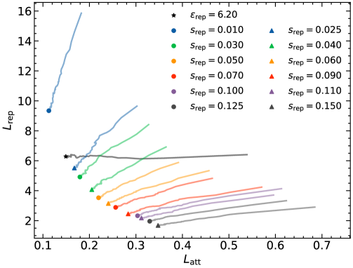
Figure 1: Identifying the Pareto front. Each colored line corresponds to the training trajectory of one model through $(L_{\text{att}},L_{\text{rep}})$ space. Models with a specified value of $s_{\text{rep}}$ use linear scalarization of the two objectives, while the model with $\epsilon_{\text{rep}}$ uses MDMM (with $\epsilon_{\text{rep}}$ denoting the constraint on $L_{\text{rep}}$).

A visual representation of track hits embedded in the learned clustering space is shown in Figure 2. While the embedding looks near-perfect to the eye, Figure 4a (discussed in the next section) confirms that this initial clustering space is still insufficient to directly reconstruct tracks from.

The graph is then built from this latent space using $k$-nearest neighbors (kNN) while also limiting the maximal edge length to $1$ (arbitrary units). To quantify the quality of the constructed graph, we call an edge true, if it connects two hits of the same particle (any edge that connects to a noise hits is false). We call an edge of interest if at least one of the two hits belongs to a particle of interest. The quality of the constructed graph vs $k$ is quantified in Figure 3 in terms of four metrics:

• Efficiency: The number of true edges of interest normalized to the number of possible true edges of interest ($\sum_{\pi\ \text{of interest}}{N_{\text{hits}}^{\pi}\choose 2}$, where $N_{\text{hits}}^{\pi}$ is the number of hits for a particle $\pi$)

• Purity: The number of true edges of interest normalized to the number of edges of interest.

• Upper bounds on figures of merit: As introduced in Ref. [5], we define upper bounds of an EC pipeline for $\epsilon^{\text{DM}}_{p_{\text{T}}>0.9}$ and $\epsilon^{\text{perfect}}_{p_{\text{T}}>0.9}$ by calculating both metrics for tracks given by the connected components of the edge-subgraph that only contains true edges. It was shown that these upper bounds do not necessarily hold for an OC pipeline, but they are still useful in quantifying the connectivity of the graph in a way that relates to the key tracking metrics.

While the overall efficiency of the GC step flattens out slowly, the upper bounds on $\epsilon^{\text{DM}}_{p_{\text{T}}>0.9}$ and $\epsilon^{\text{perfect}}_{p_{\text{T}}>0.9}$ show only very limited increases for $k>10$. We therefore choose $k=10$ for the remainder of this section. At this point, an average of $468\times 10^{3}$ edges are built with an efficiency of $77\%$, a purity of $44\%$, and EC upper bounds on $\epsilon^{\text{DM}}_{p_{\text{T}}>0.9}$ and $\epsilon^{\text{perfect}}_{p_{\text{T}}>0.9}$ of $98\%$ and $92\%$.

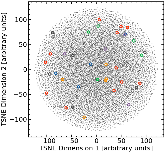
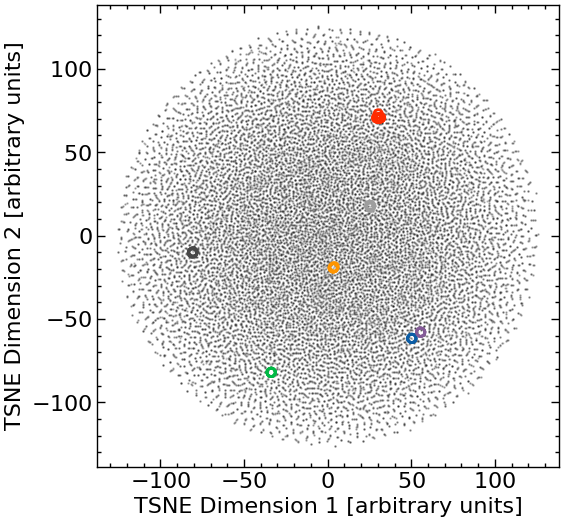
Figure 2: t-SNE projection of the input space (left) and the graph construction embedding space $h^{\text{GC}}$ (right). The hits of seven randomly selected particles of interest have been colored.

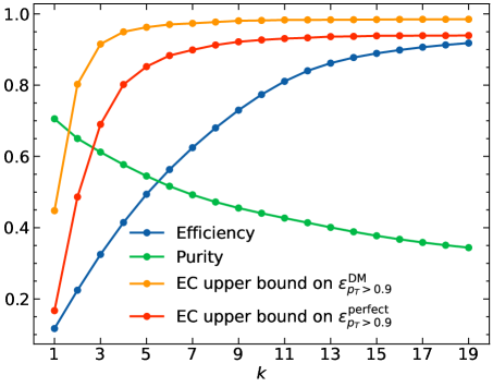
Figure 3: Choosing the number of nearest neighbors ($k$) for graph construction in our 2.0 pipeline. Note that efficiency and purity are relative to a fully connected graph of all hits per particle (rather than a path-graph of layer-to-layer connections).

3.2 Object condensation

The GNN used to perform OC is identical to that in Ref. [5] except for different input shapes and an additional residual connection that connects the 8-dimensional embedding space ($h_{i}^{\mathrm{GC}}$) that was used for GC with the final OC output coordinates.

The model is built from interaction network layers [9] with residual connections in the node updates. The node features $x_{i}^{(0)}$ are the input features $z_{i}^{(0)}\in\mathbb{R}^{14}$ described in section 2 concatenated with the GC embedding $h^{\text{GC}}_{i}\in\mathbb{R}^{8}$, i.e., $x_{i}^{(0)}\coloneqq[z_{i}^{(0)},h^{\text{GC}}_{i}]$. The edge features $e_{ij}^{(0)}$ ($(i,j)\in I$, where $I$ represents the edges of the graph) are given by $e_{ij}^{(0)}\coloneqq[x_{i}^{(0)}-x_{j}^{(0)},x_{i}^{(0)}+x_{j}^{(0)}]\in\mathbb{R}^{44}$.

Node and edge features are first encoded, $x_{i}^{(1)}\coloneqq W^{\text{enc}}_{\text{node}}x_{i}^{(0)}$, $e_{ij}^{(1)}\coloneqq W^{\text{enc}}_{\text{edge}}e_{ij}^{(0)}$, $W^{\text{enc}}_{\text{node}}\in\mathbb{R}^{192\times 22}$, and $W^{\text{enc}}_{\text{edge}}\in\mathbb{R}^{192\times 44}$. Then, five iterations of message passing are performed with

$$\begin{split}e_{ij}^{(k+1)}&\coloneqq\bigl{(}\Phi^{(k+1)}\circ\operatorname{ReLU}\bigr{)}\Big{(}\bigl{[}x_{i}^{(k)},x_{j}^{(k)},e_{ij}^{(k)}\bigr{]}\Big{)},\\ x_{i}^{(k+1)}&\coloneqq\sqrt{\beta}\,\Psi^{(k+1)}\Bigl{(}\bigl{[}\operatorname{ReLU}\bigl{(}x_{i}^{(k)}\bigr{)},{\textstyle\sum\nolimits_{j\in\mathcal{N}_{i}}}e_{ij}^{(k+1)}\bigr{]}\Bigr{)}+\sqrt{1-\beta}\,x_{i}^{(k)}.\end{split}$$ (2)

Here, $(i,j)\in I$, $k=1,\dots,5$, and $\mathcal{N}_{i}$ denotes the neighborhood of $i$. $\Phi$ and $\Psi$ are FCNNs with $\operatorname{ReLU}$ activations, a layer width of 192, and one hidden layer. $\beta$ has been chosen to be $0.5$. Finally, the clustering coordinates are decoded (and added to a residual from the GC space) as

$$c_{i}\coloneqq\sqrt{\beta^{\prime}}\,W^{\text{dec}}_{\text{c}}\operatorname{ReLU}(x_{i}^{(6)})+\sqrt{1-\beta^{\prime}}\,[h_{i}^{\text{GC}},0,\dots,0],$$ (3)

where we chose $\beta^{\prime}=0.5$, $W_{\text{c}}^{\text{dec}}\in\mathbb{R}^{24\times 192}$, and $h_{i}^{\text{GC}}$ is zero-padded to $\mathbb{R}^{24}$. The condensation likelihoods are decoded as $\beta_{i}\coloneqq\sigma\bigl{(}W^{\text{dec}}_{\beta}\operatorname{ReLU}(x_{i}^{(6)})\bigr{)}$, where $\sigma$ is the logistic function, and $W^{\text{dec}}_{\beta}\in\mathbb{R}^{1\times 192}$. The total number of parameters of this model is $1.9\times 10^{6}$.

To train the model, we use the object condensation loss functions [4] as described in Ref. [5] with the following hyperparameters: $s_{\beta}=0$, $s_{\text{rep}}=0.74$, and $q_{\text{min}}=0.01$.

3.3 Post-processing and results

We use Density-Based Spatial Clustering of Applications with Noise (DBSCAN) [10] to determine clusters in the OC clustering space $c$. DBSCAN is an iterative clustering algorithm with two parameters, $\epsilon$ (the size of the neighborhood of a point that is considered when merging clusters), and $k$ (minimum number of points within a neighborhood for the points to be considered a core point). In our case, $k=1,2,3$ produces equal results (this is related to the fact that clusters with less than three hits are discarded as track candidates) and $k\geq 4$ degrades performance (see Figure 4b). Therefore, all results use $k=1$. Based on Figure 4b, we choose $\epsilon=0.53$. The broad plateau in $\epsilon$ vs $\epsilon^{\text{DM}}_{p_{\text{T}}>0.9}$ shows that the clusters are well separated from each other and from noise. We obtain $\epsilon^{\text{DM}}_{p_{\text{T}}>0.9}=96.4\%$, $\epsilon^{\text{LHC}}_{p_{\text{T}}>0.9}=98.0\%$, $\epsilon^{\text{perfect}}_{p_{\text{T}}>0.9}=85.8\%$ and $f_{p_{\text{T}}>0.9}=0.9\%$. These metrics uniformly improve our previous results in Ref. [5]. All metrics are presented vs $p_{\text{T}}$ and vs $\eta$ in Figure 5.

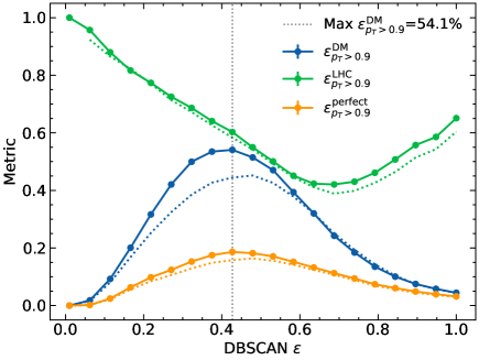
(a)

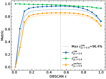
(b)

Figure 4: Rendering tracks from the learned clustering space with DBSCAN. The left plot shows track reconstruction using the embedding space $h^{\text{GC}}$ used for graph construction, and the right plot shows the significantly improved tracking performance using the OC embedding space. Dashed lines correspond to DBSCAN with $k=4$.

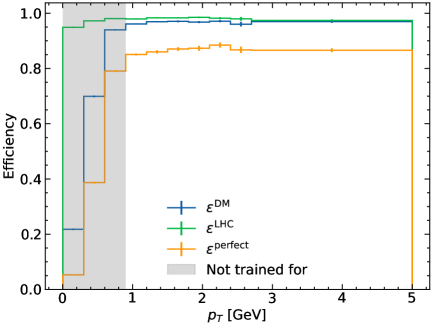
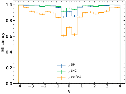
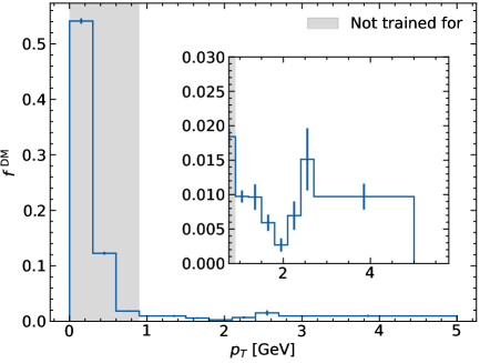
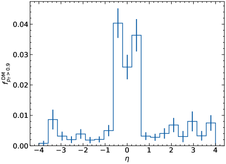
Figure 5: Tracking performance in bins of $p_{\text{T}}$ and $\eta$.

4 Progress on other architectures

While the model presented in the main part of this paper is built on interaction networks, many other architectures are left to be explored in detail. For example, GravNet [11] layers have been successfully used with an OC approach for multi-particle reconstruction in high occupancy imaging calorimeters [12, 13]. A similar architecture is also being investigated for the Belle II outer tracker, motivating studies for its suitability for an HL-LHC application. In our first experiments, we confirmed that an architecture of four (slightly modified) GravNet layers can achieve $\epsilon^{\text{DM}}_{p_{\text{T}}>0.9}>90\%$ using $k=4$ kNN with 8-dimensional latent-spaces. However, a careful optimization of hyperparameters is needed for an apples-to-apples comparison with the pipeline described in section 3.

Shifting from a very edge-oriented perspective on tracking models (e.g., EC approaches) to one that emphasizes embeddings (e.g. OC) also motivates to consider non-GNN architectures. The success of transformer architectures in encoding complex relationships between tokens and a large body of work related to hardware optimization makes this class of models attractive for the tracking problem. A key challenge for the application to tracking is to find efficient realizations of the attention mechanism in order to overcome the quadratic scaling with the attention window size (that would need to encompass all hits of an event in the naive scaled dot product attention). In our approach, this is achieved by using relative positional encoding and Exact Euclidean Locality Sensitive Hashing [14] (E2LSH) with an $\mathcal{O}(n\log n)$ scaling. The resulting model features more regular and parallelizable computations than GNN models and avoids the performance bottleneck of GPU-implementations of kNN graph building. The model is trained with contrastive learning loss functions and hard negative mining. While we are still working on detailed evaluations in terms of tracking performance, we observe up to hundred-fold inference speedups on a Quadro RTX 6000 compared to the pipeline presented in section 3.

5 Conclusions

This paper presents an object condensation approach to charged particle tracking at the worst-case pileup conditions expected at the HL-LHC. Replacing the geometric graph construction stage of our previous pipeline [5] with an adaptation of the metric learning approach from Ref. [2] allowed us to make our pipeline more streamlined while significantly improving tracking performance on the pixel detector of the TrackML dataset. Ongoing work to lower memory consumption will make it possible to apply this pipeline to the full detector. Our pipeline is part of our open-source project [15] that implements various OC tracking architectures in a modular and extensible Python package.

In addition, we discussed ongoing research into other architectures, such as GravNet and sparse transformers. The first results with sparse transformers show major improvements in inference time due to hardware-friendly implementations.

ACKNOWLEDGEMENTS

We would like to thank Javier Duarte, Peter Elmer, Philip Chang, Jonathan Guiang, David Lange, and Savannah Thais for helpful discussions and support.

References

- [1] Giuseppe Cerati et al. “Kalman Filter Tracking on Parallel Architectures” In EPJ Web of Conferences 127 EDP Sciences, 2016, pp. 00010 DOI: 10.1051/epjconf/201612700010
- [2] Xiangyang Ju et al. “Performance of a geometric deep learning pipeline for HL-LHC particle tracking” In The European Physical Journal C 81.10, 2021, pp. 876 URL: https://link.springer.com/10.1140/epjc/s10052-021-09675-8
- [3] Alina Lazar et al. “Accelerating the Inference of the Exa.TrkX Pipeline” In Journal of Physics: Conference Series 2438.1 IOP Publishing, 2023, pp. 012008 DOI: 10.1088/1742-6596/2438/1/012008
- [4] Jan Kieseler “Object condensation: one-stage grid-free multi-object reconstruction in physics detectors, graph, and image data” In The European Physical Journal C 80.9 Springer ScienceBusiness Media LLC, 2020 DOI: 10.1140/epjc/s10052-020-08461-2
- [5] Kilian Lieret and Gage DeZoort “An Object Condensation Pipeline for Charged Particle Tracking at the High Luminosity LHC”, 2023 arXiv:2309.16754 [physics.data-an]
- [6] Sabrina Amrouche et al. “The Tracking Machine Learning challenge : Accuracy phase” In The NeurIPS ’18 Competition Cham: Springer International Publishing, 2020, pp. 231–264 eprint: https://doi.org/10.1007/978-3-030-29135-8–“˙˝9
- [7] Sabrina Amrouche et al. “The Tracking Machine Learning challenge : Throughput phase” submitted to Computing and Software for Big Science In arXiv:2105.01160 [cs.LG], 2021 URL: http://arxiv.org/abs/2105.01160
- [8] John Platt and Alan Barr “Constrained Differential Optimization” In Neural Information Processing Systems 0 American Institute of Physics, 1987 URL: https://proceedings.neurips.cc/paper_files/paper/1987/file/a87ff679a2f3e71d9181a67b7542122c-Paper.pdf
- [9] Peter W. Battaglia, Razvan Pascanu, Matthew Lai, Danilo Rezende and Koray Kavukcuoglu “Interaction Networks for Learning about Objects, Relations and Physics” Preprint at https://arxiv.org/abs/1612.00222, 2016 arXiv:1612.00222 [cs.AI]
- [10] Martin Ester, Hans-Peter Kriegel, Jorg Sander and Xiaowei Xu “A density-based algorithm for discovering clusters in large spatial databases with noise.” In kdd 96.34, 1996, pp. 226–231
- [11] Shah Rukh Qasim, Jan Kieseler, Yutaro Iiyama and Maurizio Pierini “Learning representations of irregular particle-detector geometry with distance-weighted graph networks” In Eur. Phys. J. C 79.7, 2019, pp. 608 DOI: 10.1140/epjc/s10052-019-7113-9
- [12] Shah Rukh Qasim, Kenneth Long, Jan Kieseler, Maurizio Pierini and Raheel Nawaz “Multi-particle reconstruction in the High Granularity Calorimeter using object condensation and graph neural networks” https://doi.org/10.48550/arXiv.2106.01832 In arXiv:2106.01832 [physics.ins-det], 2021 URL: http://arxiv.org/abs/2106.01832
- [13] Shah Rukh Qasim, Nadezda Chernyavskaya, Jan Kieseler, Kenneth Long, Oleksandr Viazlo, Maurizio Pierini and Raheel Nawaz “End-to-end multi-particle reconstruction in high occupancy imaging calorimeters with graph neural networks” In Eur. Phys. J. C 82.8, 2022, pp. 753 arXiv:https://doi.org/10.1140/epjc/s10052-022-10665-7 [physics.ins-det]
- [14] Mayur Datar, Nicole Immorlica, Piotr Indyk and Vahab S. Mirrokni “Locality-Sensitive Hashing Scheme Based on p-Stable Distributions” In Proceedings of the Twentieth Annual Symposium on Computational Geometry, SCG ’04 Brooklyn, New York, USA: Association for Computing Machinery, 2004, pp. 253–262 DOI: 10.1145/997817.997857
- [15] Kilian Lieret and Gage DeZoort “gnn_tracking: An open-source GNN tracking project”, https://github.com/gnn-tracking/gnn_tracking