Spectral holographic trapping: Creating dynamic force landscapes with polyphonic waves

Abstract

Acoustic trapping uses forces exerted by sound waves to transport small objects along specified trajectories in three dimensions. The structure of the acoustic force landscape is governed by the amplitude and phase profiles of the sound’s pressure wave. These profiles can be controlled through deliberate spatial modulation of monochromatic waves, by analogy to holographic optical trapping. Alternatively, spatial and temporal control can be achieved by interfering a small number of sound waves at multiple frequencies to create acoustic holograms based on spectral content. We demonstrate spectral holographic trapping by projecting acoustic conveyor beams that move millimeter-scale objects along prescribed paths, and control the complexity of particle trajectories by tuning the strength of weak reflections. Illustrative spectral superpositions of static and dynamic force landscapes enable us to realize two variations on the theme of a wave-driven oscillator, a deceptively simple dynamical system with surprisingly complex phenomenology.

Forces exerted by sound waves can levitate and transport small objects without physical contact, which is a boon for processing sensitive [1] and hazardous materials [2]. The interplay of sound waves with small scatterers also provides an archetypal model for investigating the physics of wave-matter composite systems [3, 4, 5, 6]. Most implementations of acoustic trapping use sound waves of a single fixed frequency and achieve dexterous control by suitably structuring the waves’ amplitude and phase profiles with large arrays of acoustic “pixels” [7, 8]. Like holographic optical traps [9], this kind of acoustic trapping pattern is reconfigured by actively changing the wavefront structure at each pixel in the array.

Here, we draw attention to an alternative approach to dynamic acoustic trapping whose ability to move matter along prescribed paths is encoded in the spectral content of a small number of acoustic sources. We illustrate the potential utility of such spectral traps by demonstrating dynamic acoustic manipulation along a single axis using just two acoustic pixels emitting stationary sound fields.

I Acoustic Forces

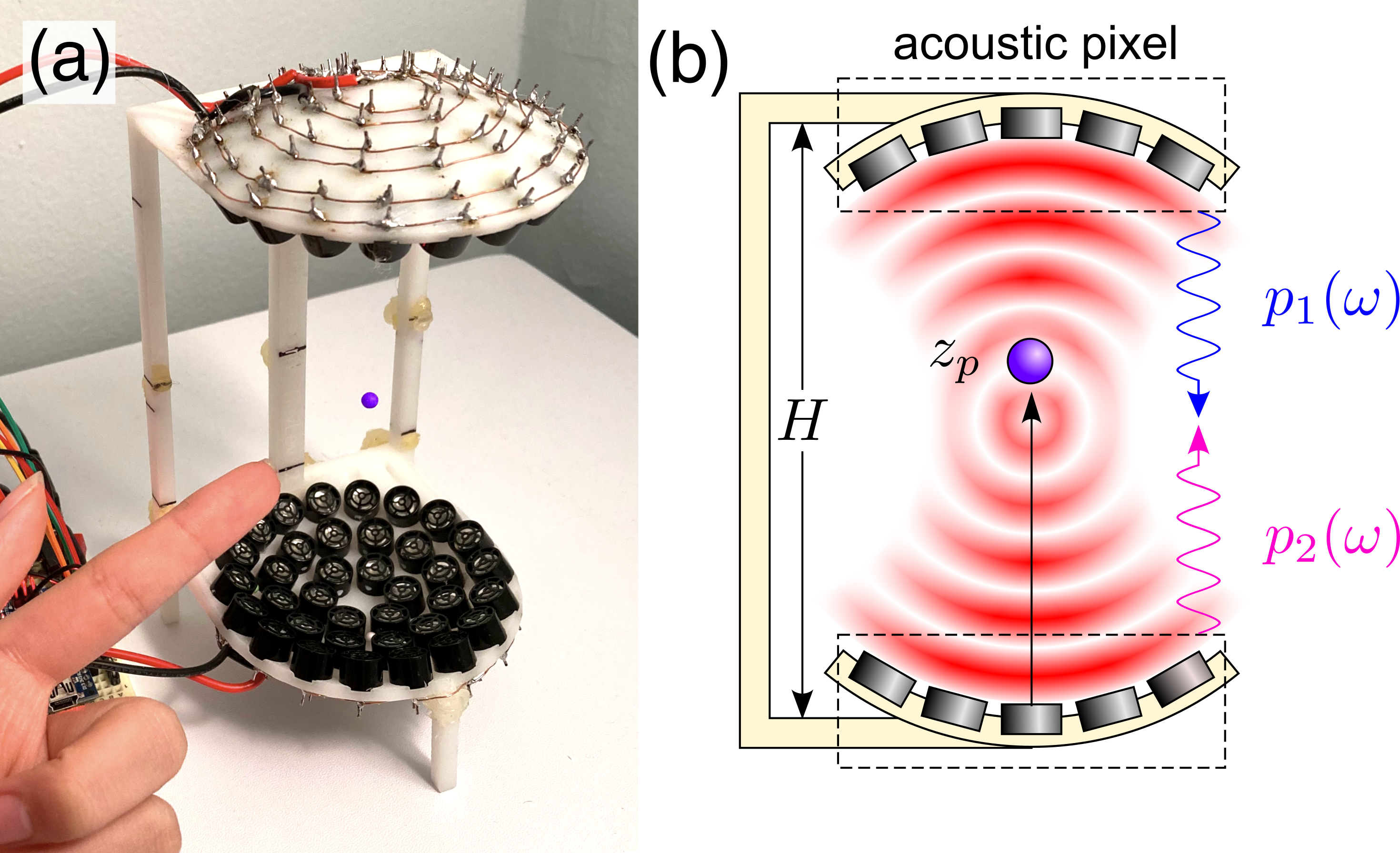
Figure 1: (a) Acoustic trap holding a single millimeter-scale particle in air at a carrier frequency of $f=$40\text{\,}\mathrm{kHz}$$. (b) Schematic representation of spectral holographic trapping. Two acoustic pixels project counterpropagating pressure waves, $p_{1}(\omega)$ and $p_{2}(\omega)$, into a spherical cavity of height $H$. Dense rigid particles can be trapped at nodes in the combined pressure field. The traps’ positions evolve in time based on the spectral content of the two projected waves.

A steady sound wave at frequency $\omega$ propagating through an incompressible medium can be characterized by the real-valued amplitude profile, $u(\bm{r})$, and phase profile, $\phi(\bm{r})$, of its pressure field:

$$p(\bm{r},t)=u(\bm{r})\,\exp\left(i\phi(\bm{r})\right)\,\exp(-i\omega t).$$ (1)

This structured wave can be decomposed into plane waves whose wave number satisfies the standard dispersion relation, $k=\omega/c_{m}$, where $c_{m}$ is the speed of sound in the medium. A small particle at position $\bm{r}$ in this field experiences a time-averaged acoustic force [10, 11]

$$\bm{F}(\bm{r})=-\nabla U_{G}(\bm{r})+\mathcal{O}\left\{(ka_{p})^{3}\right\},$$ (2a)

to leading order in the particle’s dimensionless size scale, $$ka_{p}<1$$, where

$$U_{G}(\bm{r})=\frac{1}{4}\,A\,u^{2}+\frac{1}{8k^{2}}\,B\,\nabla^{2}u^{2}$$ (2b)

is the classic Gor’kov potential [12, 11]. The force landscape described by Eq. (2) depends only on the pressure wave’s amplitude profile, and is is manifestly conservative if $u(\bm{r})$ itself does not depend on time. The phase profile, $\phi(\bm{r})$, governs nonconservative acoustic radiation forces [11] that may be neglected for sufficiently small particles, and vanish identically in standing waves.

For the specific case of a spherical particle of radius $a_{p}$, the coefficients $A$ and $B$ depend on the particle’s density, $\rho_{p}$, and sound speed, $c_{p}$, relative to those of the medium as [12]

$$A =\frac{4\pi}{3}a_{p}^{3}\,\kappa_{m}\left(f_{0}-\frac{3}{2}f_{1}\right)\quad\text{and}$$ (3a)

$$B =-2\pi a_{p}^{3}\,\kappa_{m}\,f_{1},$$ (3b)

where the monopole coupling coefficient,

$$f_{0}=1-\frac{\kappa_{p}}{\kappa_{m}},$$ (3c)

gauges the mismatch in isentropic compressibility between the particle, $$\kappa_{p}=(\rho_{p}c_{p}^{2})^{-1} \kappa_{m}=(\rho_{m}c_{m}^{2})^{-1}$$, and the medium, , and the dipole coupling coefficient,

$$f_{2}=\frac{\rho_{p}-\rho_{m}}{\rho_{p}+\frac{1}{2}\rho_{m}},$$ (3d)

accounts for the mismatch in density.

II Dynamic Acoustic Trapping with Spectral Holograms

A superposition of sound waves can be expressed in the form of Eq. (1), with $u(\bm{r})$ and $\varphi(\bm{r})$ representing the amplitude and phase of the associated interference pattern. This approach has been used to create holographic acoustic traps [13, 14, 15, 7, 16, 17], typically by superposing waves of the same frequency emanating from large arrays of sources. Dynamic trapping patterns are created by suitably modifying the amplitudes and phases of the individual sources over time [17].

Alternatively, time-varying acoustic force landscapes can be created by superposing steady sound waves at different frequencies; the resulting beats manifest as slow time variations of the Gor’kov potential. Equation (2) captures this behavior by implicitly averaging the acoustic force over one period, $T=2\pi/\omega$, of the carrier frequency, $\omega$. The spectral content of a polyphonic superposition can replace the spatiotemporal variations in a standard acoustic hologram to create dynamic acoustic traps. We refer to this frequency-based approach to wavefront shaping as “spectral holography”.

To illustrate the opportunities created by spectral holography, we demonstrate programmable transport along one spatial dimension using force landscapes created with just two acoustic pixels. Our experimental system, illustrated in Fig. 1, was introduced by Marzo, Barnes and Drinkwater [18] and consists of two banks of ultrasonic transducers operating in air at a nominal frequency of $40\text{\,}\mathrm{kHz}$. Each bank acts as a single acoustic pixel, projecting sound into a cylindrical section of a spherical cavity of diameter $H=$10\text{\,}\mathrm{cm}$$. The counterpropagating waves interfere within the cavity to create alternating nodes and antinodes of the pressure field along the central axis.

II.1 Diphonic Acoustic Conveyor

If both sources operate at the same frequency, $\omega$, their interference creates a standing wave with axial nodes separated by half a wavelength. Each node acts as a potential energy well for small incompressible particles, such as the expanded polystyrene bead shown in Fig. 1(a).

Detuning the two sources by $\Delta\omega\ll\omega$ creates beats in the axial pressure field,

$$p(z,t)=2p_{0}\,\cos\left(kz-\frac{\Delta\omega}{2}t\right)\,\cos\left(\frac{\Delta\omega}{2c_{m}}z-\omega t\right),$$ (4)

that manifest themselves as motion of the time-averaged axial force field,

$$\bm{F}_{a}(z,t)=F_{0}(\omega)\,\sin(2kz-\Delta\omega\,t)\,\hat{z},$$ (5)

after substitution into Eq. (2). The prefactor,

$$F_{0}(\omega)=(A-2B)\,kp_{0}^{2},$$ (6)

is positive for dense incompressible particles, which therefore tend to be trapped at the nodes of the pressure field. The entire force landscape moves along $\hat{z}$ at a steady speed,

$$v_{c}=c_{m}\,\frac{\Delta\omega}{2\omega},$$ (7)

that is proportional to the detuning, $\Delta\omega$. Setting aside complications due to inertia and drag [19, 20, 21, 22], trapped particles should travel along with the landscape,

$$z_{p}(t)\approx z_{n}(t)$$ (8)

where $z_{n}(t)=z_{n}(0)+v_{c}t$ is the position of the $n$-th pressure node at time $t$. This type of traveling force landscape is known as a “conveyor” [23, 24, 25, 18, 26, 27] and is the simplest example of a spectral hologram.

The data in Fig. 2(a) demonstrate an acoustic conveyor transporting a millimeter-scale bead composed of type II expanded polystyrene (EPS) foam with a measured [22] mass density of $\rho_{p}=$30.5\pm 0.2\text{\,}\mathrm{kg}\text{\,}{\mathrm{m}}^{-3}$$. The particle’s trajectory is recorded at $170\text{\,}\mathrm{f}\mathrm{r}\mathrm{a}\mathrm{m}\mathrm{e}\mathrm{s}\mathrm{/}\mathrm{s}$ with a monochrome video camera (FLIR, Blackfly S USB3) whose $5\text{\,}\mathrm{ms}$ exposure time is fast enough to avoid motion blurring given the system magnification of $61\text{\,}\mathrm{\SIUnitSymbolMicro}\mathrm{m}\mathrm{/}\mathrm{p}\mathrm{i}\mathrm{x}\mathrm{e}\mathrm{l}$. Each frame in a video sequence is thresholded with Otsu’s method, and the particle’s position is computed as the center of mass of the resulting simply-connected cluster of foreground pixels. The image of a typical particle yields a $1000$-pixel cluster whose axial centroid, $z_{p}(t)$, can be located with an estimated accuracy [22] of $\Delta z_{p}=$0.17\text{\,}\mathrm{p}\mathrm{i}\mathrm{x}\mathrm{e}\mathrm{l}$=$10\text{\,}\mathrm{\SIUnitSymbolMicro m}$$, which suffices for our application.

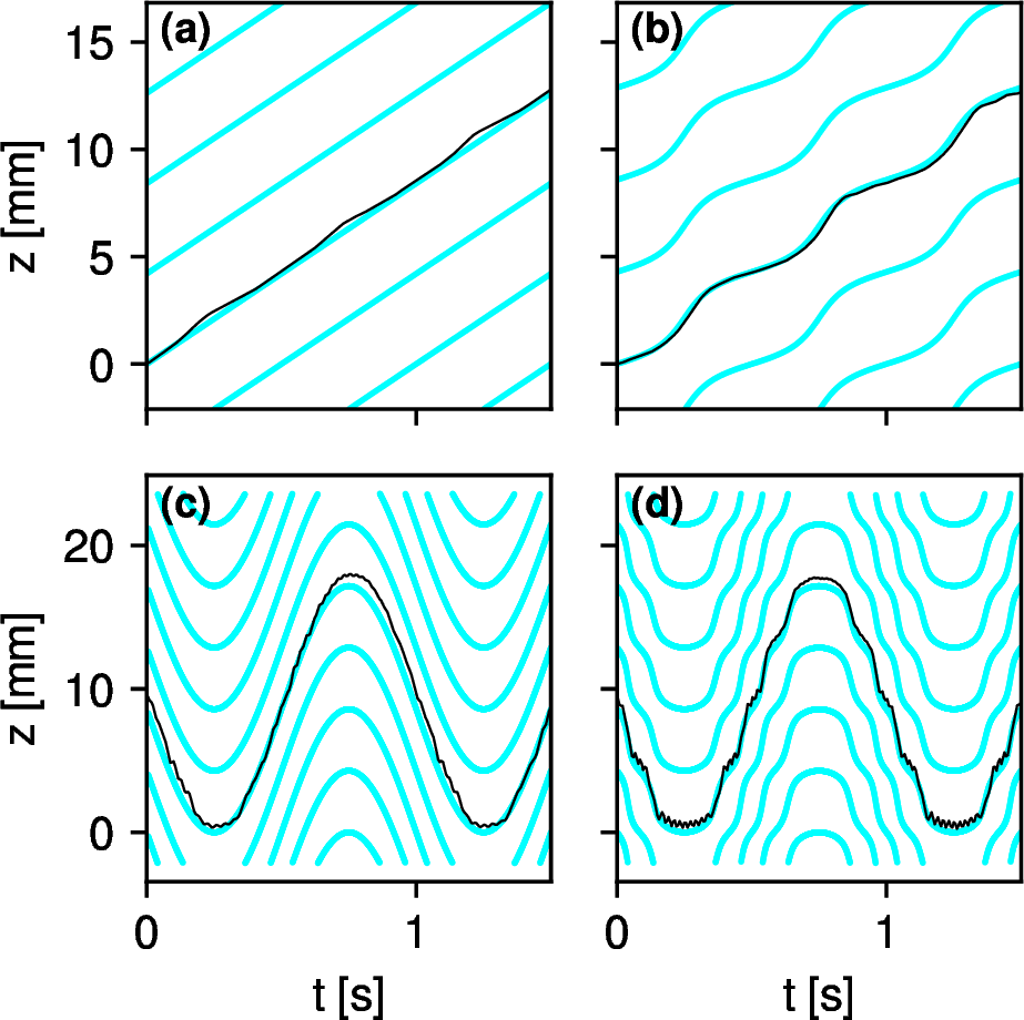
Figure 2: Measured trajectories (black curves) for a $2\text{\,}\mathrm{mm}$-diameter EPS bead (a) and (b) in an acoustic conveyor, and (c) and (d) in an acoustic scanner. These are compared with predictions of Eq. (14) for $\epsilon_{0}=$0.38$$ (cyan curves). (b) and (d) Tuning the carrier frequency to a cavity resonance at $f=\omega/(2\pi)=$40.0\pm 0.1\text{\,}\mathrm{kHz}$$ creates a standing wave that modulates the trajectory. (a) and (c) Detuning to $f=$40.7\text{\,}\mathrm{kHz}$$ suppresses the standing wave. Conveyor: $\Delta f=\Delta\omega/(2\pi)=$2\text{\,}\mathrm{Hz}$$. Scanner: $\Delta\phi=$720\text{\,}\pi$$.

II.2 Polyphonic Acoustic Scanner

More sophisticated modes of transport can be achieved with more sophisticated superpositions of tones. Such a generalized conveyor, which we call a “scanner”, can be implemented as the superposition of waves from two sources, as depicted in Fig. 1(b), with time-varying relative phase,

$$p_{1}(t) =p_{0}\,e^{i\omega t}$$ (9a)

$$p_{2}(t) =p_{0}\,e^{i\varphi(t)}\,e^{-i\omega t}.$$ (9b)

Such a superposition creates a time-averaged force landscape,

$$\bm{F}_{a}(z,t)=F_{0}(\omega)\,\sin(2kz-\varphi(t))\,\hat{z},$$ (10)

whose traps travel along $\hat{z}$ as

$$z_{n}(t)=z_{n}(0)-\frac{1}{2k}\,\varphi(t).$$ (11)

The resulting motion is slow in the sense that relevant variations in the relative phase satisfy $\left|\dot{\varphi}\right|\ll\omega$, where the dot refers to a derivative with respect to time. Any faster variations are suppressed in theory by the implicit time average in Eq. (2) and physically by viscous drag and the particle’s inertia.

Active control of the relative phase, $\varphi(t)$, has been used in the context of holographic optical trapping to project optical conveyors [23] and optical tractor beams [25], and more recently has been used to demonstrate acoustic conveyors [18]. Rather than actively sweeping the phase, however, we instead can decompose $\varphi(t)$ into its spectral components and use those to create a scanner that operates in steady state without active intervention. For example, a sinusoidal scanner described by $\varphi(t)=\Delta\phi\,\sin(\Omega t)$ can be implemented through the Jacobi-Anger identity,

$$p_{2}(t)=p_{0}\,\sum_{n=-\infty}^{\infty}J_{n}(\Delta\phi)\,e^{i(n\Omega-\omega)t},$$ (12)

which specifies the frequencies needed to implement the scanner and their relative amplitudes. A working example can be projected with just the first few orders, $n\in[-4,4]$. The resulting spectral hologram then transports trapped objects back and forth continuously and smoothly without active intervention. The data in Fig. 2(c) show such a scanner in action.

II.3 Spectral Superposition of Static and Dynamic Landscapes

Acoustic pixels are actively driven transducers. As a consequence, they not only project sound waves, but also act as absorbing boundary conditions for incident waves [28]. This feature has not been emphasized in previous acoustic-trapping studies [18]. Active cancellation of reflections enables the counterpoised acoustic pixels in an instrument such as the example in Fig. 1 to create standing-wave acoustic traps even when the carrier frequency, $\omega$, is not tuned to a cavity resonance.

In practice, acoustic pixels reflect a small proportion, $\epsilon_{0}$, of incident sound waves. Reflections contribute to the force landscape by forming standing waves within the cavity whose amplitude can be controlled through the choice of $\omega$. The associated force landscape therefore has both time-varying and stationary components,

$$\bm{F}(\bm{r},t)=\bm{F}_{a}(\bm{r},t)+\bm{F}_{s}(\bm{r}),$$ (13a)

where the standing-wave contribution is approximately

$$\bm{F}_{s}(\bm{r})\approx 2\,\epsilon(\omega)\,F_{0}(\omega)\,\sin(2kz)\,\hat{z}.$$ (13b)

The factor of $$2$$ in Eq. (13b) accounts for the independent contributions from each of the pixels. The depth of the stationary landscape’s modulation,

$$\epsilon(\omega)=\epsilon_{0}\,\cos\bigg{(}\frac{2H}{c_{m}}\omega\bigg{)},$$ (13c)

is proportional to the acoustic pixels’ reflection coefficient, $\epsilon_{0}$, and can be tuned by adjusting the carrier frequency. For the cavity depicted in Fig. 1, we find that particle trajectories are consistent with $\epsilon_{0}=$0.38\pm 0.02$$. The overall scale of the stationary force landscape is set by $F_{0}(\omega)$, which is given by Eq. (6).

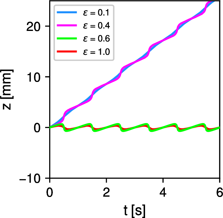
Figure 3: Simulated trajectories of the particle from Fig. 2 in a spectrally superposed acoustic conveyor, Eq. (13), as a function of the cavity reflection coefficient, $\epsilon(\omega)$. Conveyor detuning: $\Delta f=\Delta\omega/(2\pi)=$1\text{\,}\mathrm{Hz}$$.

If the reflection coefficient is large enough, $\epsilon_{0}>0.5$, the central frequency can be tuned so that $2\epsilon(\omega)>1$. In that case, the standing wave exerts enough force to trap the particle, and the dynamic landscape acts as a time-dependent perturbation. Representative trajectories for this mode of motion are plotted in Fig. 3 as a function of $\epsilon(\omega)$.

In the opposite limit of weak reflections, $\epsilon(\omega)<0.5$, the particle is transported by the moving conveyor across the stationary landscape. The nodes then trace out trajectories,

$$z_{n}(t|\epsilon(\omega))=z_{n}(0)-\frac{1}{k}\,\arctan\left(\frac{\epsilon(\omega)-1}{\epsilon(\omega)+1}\tan\left(\frac{\varphi(t)}{2}\right)\right),$$ (14)

that reduce to Eq. (11) when $\epsilon(\omega)=0$. This mode of motion also is plotted in Fig. 3 and is consistent with the perturbed trajectories observed experimentally in Fig. 2(b) and Fig. 2(d).

The particles’ trajectories increasingly deviate from the traps’ trajectories as $\epsilon(\omega)$ approaches $1/2$ and the trajectories become increasingly sinuous. We quantify these deviations with the kinematic variance,

$$\sigma^{2}(\omega)=\frac{1}{T}\int_{0}^{T}[z_{p}(t)-z_{n}(t)]^{2}\,dt,$$ (15)

which is plotted as a function of the carrier frequency, $\omega$, in Fig. 4(a). Measurements are compared with the prediction obtained by setting $z_{p}(t)=z_{n}(t|\epsilon(\omega))$, which is plotted as a solid curve. The kinematic model is consistent with the measurement when the carrier frequency is tuned away from the cavity resonance so that the particle travels smoothly at constant speed. Tuning to the cavity resonance at $f=$40.2\text{\,}\mathrm{kHz}$$ maximizes the particle’s acceleration and increases deviations between the trajectories of the particle and the trap. These discrepancies can be resolved by accounting for inertial corrections to the viscous drag acting on the particle.

III Accounting for Inertia and Drag

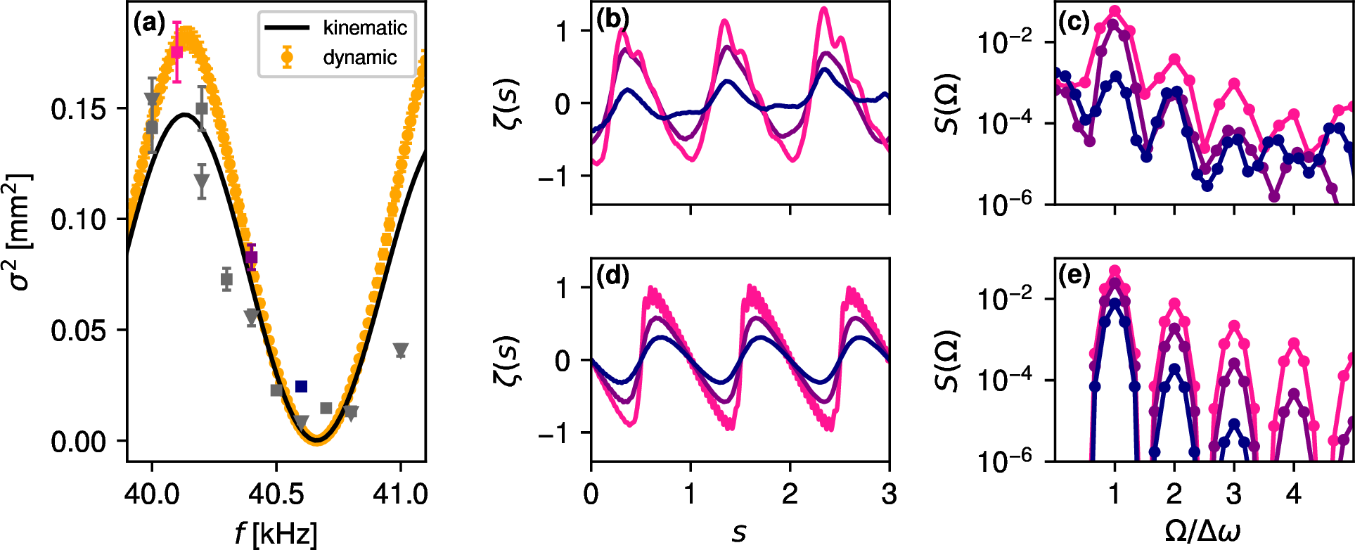
Figure 4: (a) Variance of excursions from the mean conveyor trajectory as a function of carrier frequency. Measurements are plotted as discrete points. Solid curves denote analytic predictions of Eq. (14) (black) and numerical solutions to Eq. (19) (orange). (b) Typical measured trajectories colored to match corresponding points in (a). (c) Power spectra of the trajectories in (b) showing the growth of harmonics in the particle’s trajectory as the depth of modulation increases. (d) and (e) numerical solutions of Eq. (19) for the same set of conditions. Conveyor detuning frequency: $\Delta f=\Delta\omega/2\pi=$2\text{\,}\mathrm{Hz}$$.

A trapped particle hews to the trajectory of its acoustic trap if the motion is slow enough to neglect the inertia of the fluid medium [22]. More generally, the equation of motion for a particle of mass $m_{p}$,

$$m_{p}\ddot{z}_{p}=F_{a}(z_{p},t)+F_{s}(z_{p})+F_{d}(\dot{z}_{p},\ddot{z}_{p}),$$ (16)

reflects contributions from the active force landscape, the stationary force landscape and viscous drag, respectively. A sphere of radius $a_{p}$ moving through a fluid of viscosity $\eta_{m}$ and mass density $\rho_{m}$ experiences a drag force that is described by the Basset-Boussinesq-Oseen equation [29, 19, 30, 21],

$$F_{d}(\dot{z}_{p},\ddot{z}_{p})=6\pi\eta_{m}a_{p}\left[\dot{z}_{p}+\tau\ddot{z}_{p}+\sqrt{\frac{9\tau}{\pi}}\int_{-\infty}^{t}\frac{\ddot{z}_{p}(t^{\prime})}{\sqrt{t-t^{\prime}}}\,dt^{\prime}\right],$$ (17a)

which accounts for the inertia of the displaced fluid on time scales set by the viscous relaxation time,

$$\tau=\frac{\rho_{m}}{9\eta_{m}}\,a_{p}^{2}.$$ (17b)

The history-dependent contribution to the drag complicates an analytic formulation of the transport properties for a general spectral hologram. To illustrate the challenge, we consider the comparatively simple case of a particle moving under the influence of an acoustic conveyor. Competition between the active and stationary force landscapes causes the particle to oscillate at the beat frequency, $\Delta\omega$, about the moving trap’s position. We therefore define the dimensionless displacement in the co-moving frame,

$$\zeta(t)=2kz_{p}(t)-\begin{cases}\Delta\omega\,t,&\epsilon(\omega)<0.5\\ 0,&\epsilon(\omega)>0.5\end{cases}.$$ (18)

Applying Eq. (16) and Eq. (17) then yields the deceptively simple dimensionless equation of motion,

$$\zeta^{\prime\prime}+b\,\zeta^{\prime}+\zeta=\tilde{\epsilon}\sin\left(\zeta-\frac{\Delta\omega}{\omega_{0}}\,s\right),$$ (19)

where primes denote derivatives with respect to the dimensionless time, $s=\omega_{0}t$. Equation (19) describes a wave-driven oscillator [31] whose exceptionally rich phenomenology only recently has been brought to light. Wave-driven oscillators differ from more familiar nonlinear dynamical systems, such as the Duffing oscillator [32, 33], because its spatial nonlinearity is irreducibly coupled to the time dependence of the driving.

The effective driving strength in Eq. (19),

$$\tilde{\epsilon}(\omega)=\begin{cases}2\epsilon(\omega),&\epsilon(\omega)<0.5\\ \frac{1}{2\epsilon(\omega)},&\epsilon(\omega)>0.5\end{cases},$$ (20)

can be varied over the range $\tilde{\epsilon}(\omega)\in[0,1]$ by adjusting the carrier frequency relative to the cavity resonance. Similarly, the natural frequency,

$$\omega_{0}(\omega)=\sqrt{\frac{2kF_{0}}{m}}\times\begin{cases}1,&\epsilon(\omega)<0.5\\ \sqrt{2\epsilon(\omega)},&\epsilon(\omega)>0.5\end{cases},$$ (21)

and the drag coefficient,

$$b(\omega)=\frac{6\pi\eta_{m}a_{p}}{m\,\omega_{0}}\times\begin{cases}1,&\epsilon(\omega)<0.5\\ (2\epsilon(\omega))^{-1},&\epsilon(\omega)>0.5\end{cases},$$ (22)

both depend on cavity tuning when $\epsilon(\omega)>0.5$.

Equations (21) and (22) incorporate the inertial corrections from Eq. (17) by introducing the dynamical mass [19, 20, 22],

$$m(\Delta\omega)=m_{p}\left\{1+\frac{1}{2}\frac{\rho_{m}}{\rho_{p}}\left[1+\frac{9}{2}\frac{\delta(\Delta\omega)}{a_{p}}\right]\right\},$$ (23a)

under the simplifying assumption the particle oscillates harmonically at the driving frequency, $$\Delta\omega$$. The sphere’s effective mass is increased in this approximation by the mass of the fluid in a Prandtl-Schlichting boundary layer of thickness [19]

$$\delta(\Delta\omega)=\sqrt{\frac{2\eta_{m}}{\rho_{m}}\frac{1}{\Delta\omega}}.$$ (23b)

This correction has been demonstrated to quantitatively model the damped oscillations of a particle levitated in a static acoustic trap [22]. For particles moving in an acoustic conveyor, the dynamic model more accurately accounts for the magnitude of measured fluctuations, as can be seen in Fig. 4(a).

Measured acoustic-conveyor trajectories in Fig. 4(b) and their power spectra in Fig. 4(c) are reproduced reasonably well by the numerical solutions of Eq. (19) that are plotted in Fig. 4(d) and Fig. 4(e). These examples illustrate the effect of tuning the carrier frequency on the amplitude and harmonic content of the particle’s dynamic response. Values of $F_{0}$ and $m_{0}$ used for the numerical solutions are obtained from measured trajectories using the analytical approach described in Ref. [22]. The power spectra are computed as

$$S(\Omega)=\left|\int_{0}^{1}\zeta(s)\,W(s)\,e^{-i\Omega s}\,ds\right|^{2},$$ (24)

using the Blackman-Harris window function, $W(s)$. The wave-driven oscillator responds most strongly at the driving frequency, $\Omega=\Delta\omega$. Increasingly much power is directed into harmonics of that driving frequency as the depth of modulation increases. Agreement between the measured and computed power spectra illustrates the utility of the Basset-Boussinesq-Oseen equation for interpreting the behavior of wave-driven oscillators created with sound. At the same time, the presence of strong harmonics suggests even better agreement could be attained by seeking self-consistent solutions to the equation of motion, including the BBO correction described in Eq. (17).

More generally, the wave-driven oscillator has been shown [31] to respond at both harmonics and subharmonics of the driving frequency and to undergo transitions between subharmonic states depending on the strength of the driving, $\tilde{\epsilon}(\omega)$, the strength of the damping, $b(\omega)$ and the relationship between the driving frequency, $\Delta\omega$, and the oscillator’s natural frequency, $\omega_{0}$. Transitions between subharmonic states feature both period-doubling routes to chaos and Fibonacci cascades [31]. No complete description of the wave-driven oscillator is yet available, even in the weak-driving regime, $\tilde{\epsilon}<1$. Previous experimental and numerical studies [31], furthermore, have neglected the inertial corrections described by Eq. (17) that are likely to have influenced their results. Future studies of the wave-driven oscillator and related dynamical systems would benefit both from the streamlined experimental implementation afforded by spectral holography and also from the analytical approach discussed here.

IV Discussion

Spectral holographic trapping uses interference among waves at multiple frequencies to create time-averaged force landscapes that evolve dynamically on the inertial time scales of trapped objects. Spatiotemporal control afforded by the frequency content of the projected waves reduces the complexity of acoustic manipulation systems by replacing the many spatial degrees of freedom required for conventional monotonic holographic projection. Spectral holography therefore allows complex force landscapes to be generated with small numbers of acoustic pixels. We have demonstrated two archetypal examples, a unidirectional conveyor created with two frequencies and a bidirectional scanner created with nine. We also have shown that tuning the carrier frequency to cavity resonances can usefully implement a superposition of dynamic and static force fields with no additional complexity. In the case of an acoustic conveyor, this superposition implements a wave-driven oscillator whose exceedingly rich dynamical properties emerge from an interplay between the acoustic force field, the particle’s inertia and viscous drag in the supporting medium. This study also highlights the importance of accounting for the fluid’s inertia when planning and interpreting the motions of particles in acoustic force landscapes.

The combination of rich spectral control and analytic dynamical modeling expands the prospects for dexterous acoustic manipulation of macroscopic materials. The present study has focused on the dynamics of individual particles in spectral holograms created within cavities. Additional opportunities can be imagined for free-space manipulation with traveling waves and for self-organization guided by wave-mediated interactions in many-body systems immersed in spectral holograms.