PCDP-SGD: Improving the Convergence of Differentially Private SGD via Projection in Advance

Abstract

The paradigm of Differentially Private SGD (DP-SGD) can provide a theoretical guarantee for training data in both centralized and federated settings. However, the utility degradation caused by DP-SGD limits its wide application in high-stakes tasks, such as medical image diagnosis. In addition to the necessary perturbation, the convergence issue is attributed to the information loss on the gradient clipping. In this work, we propose a general framework PCDP-SGD, which aims to compress redundant gradient norms and preserve more crucial top gradient components via projection operation before gradient clipping. Additionally, we extend PCDP-SGD as a fundamental component in differential privacy federated learning (DPFL) for mitigating the data heterogeneous challenge and achieving efficient communication. We prove that pre-projection enhances the convergence of DP-SGD by reducing the dependence of clipping error and bias to a fraction of the top gradient eigenspace, and in theory, limits cross-client variance to improve the convergence under heterogeneous federation. Experimental results demonstrate that PCDP-SGD achieves higher accuracy compared with state-of-the-art DP-SGD variants in computer vision tasks. Moreover, PCDP-SGD outperforms current federated learning frameworks when DP is guaranteed on local training sets.

1 Introduction

As the importance of preserving the privacy of training data gains increased attention [10], the widely adopted privacy-preserving optimizer DP-SGD [1] has found extensive applications in both centralized [26, 31, 16] and federated settings [37, 27] for providing privacy guarantees over training samples. Essentially, the DP-SGD optimizer achieves the differential privacy (DP) [15] through per-sample gradient clipping to limit the sensitivity within the $l_{2}$ norm threshold before perturbation. Unfortunately, the performance of the DP-SGD model drops due to the gradient clipping and perturbation, which makes it hard to apply for high-stakes tasks such as medical image diagnosis [46, 2], autonomous driving [14, 7], and biometric identification [20, 32].

For improving the utility-privacy trade-off, existing works mainly focus on the operations after the per-sample clipping. For example, based on the observation that the empirical gradient during training is concentrated in the top subspace [17, 22, 25, 34], a line of work [43, 16] projects the gradients with $d$ dimensions into the top-$k$ eigenspace after clipping, and succeeds in decoupling the high-dimensional dependence of DP noise from $\mathcal{O}(\sqrt{d})$ to $\mathcal{O}(\sqrt{k})$. In addition, to evade the privacy restriction [3, 5], introducing the public auxiliary dataset to generate the top-$k$ eigenspace as projection has become a prevailing strategy. Moreover, Chen et al. [11] provide a theoretical analysis of gradient clipping for Abadi’s clipping function [1] based on the symmetry assumption, where the clipping threshold is converted into the clipping probability, and obtain the effect of clipping bias on the convergence of DP-SGD. However, existing works have not explicitly inspected how pre-processing on gradients before clipping benefits the convergence of DP-SGD.

Orthogonal to these approaches, we investigate the convergence gain from a pre-clipping operation with theoretical analysis. Intuitively, over the optimization of the deep networks, the spectrum of gradients can characterize the loss landscape [22, 25, 17]. This spectrum separates into a few top gradient components with large positive eigenvalues, which play a dominant role in the optimization, and bulk ambient gradient components with small eigenvalues. Typically, the gradient clipping in DP-SGD scales each dimension of the gradient uniformly with an $l_{2}$ norm limit, but counting ambient gradient components into the per-sample gradient norm is not cost-effective as they change very little. We notice that projection can be regarded as a a pre-processing method, identifying the top-$k$ gradient components, weeding out the ambient gradient components, and thus compressing the gradient $l_{2}$ norm to fit the clipping bound better. Thus, with the support of the top subspace assumption, we are motivated to propose the PCDP-SGD framework and improve the convergence by utilizing the public-based projection before clipping to ignore ambient gradient components and avoid over-clipping on top components.
Clipping solely the crucial components, rather than each dimension, is more productive. Specifically, to visually explain this mind, we present a schematic diagram in Fig. 1 where we assume that a sample gradient $g$ can be divided into top component $g_{u_{1}}$ and ambient component $g_{u_{2}}$ in its eigenspace. Actually, as shown in Fig. 1(a), Abadi’s clipping incorporates the $l_{2}$ norm of $g_{u_{1}}$ and $g_{u_{2}}$ into the clipping bound $c$, causing $g_{u_{1}}$ to be clipped. On the contrary, our mechanism excludes the ambient gradient component $g_{u_{2}}$ (dissolved in Fig. 1(b) with dashed line) and only retains the top component $g_{u_{1}}$ with minimal information loss. From the probability perspective [11], the freezing of clipping in PCDP-SGD narrows clipping bias, i.e., $1-P(\|g_{u_{1}}\|_{2}\leq c)\leq 1-P(\|g_{u_{1}}+g_{u_{2}}\|_{2}\leq c)$, which promotes convergence in theory. In a word, our pre-projection method facilitates greater preservation of the top component under the same clipping threshold, in contrast to the scenario without pre-projection, resulting in improved utility at an equivalent noise level.
As a general privacy-preserving module, PCDP-SGD could also be adopted by the local end in federated learning settings to provide local DP guarantee for released local model updates. We demonstrate that PCDP-SGD achieves higher accuracy and low communication cost in FL, as it mitigates the notorious challenges of data heterogeneity and uploading only crucial components. Specifically, we prove that a public projection subspace for federated clients can relieve the local drifts by constraining the divergence of local gradient descent, which plays a critical role in non-IID settings. In addition, federated clients can reduce dimensions and upload local gradients through projection to achieve efficient communication.
We summarize our contributions in this work as follows:

• We introduce a general framework PCDP-SGD that preserves crucial eigen dimensions and enhances convergence by incorporating a pre-projection step prior to gradient clipping under centralized and federated settings.

• In the centralized scenario, we provide the practical projection reconstruction error theory, analyze the improvement in convergence caused by pre-projection, and elaborate on the clipping bias correction with projection.

• In the federated scenario, PCDP-SGD primarily alleviates data heterogeneity and achieves efficient communication. We also provide clipped convergence with sample-level DP.

• We verify that PCDP-SGD outperforms other DP-SGD variants under the high-privacy regime. Our experimental analysis offers a holistic perspective on enhancing performance under DP and data heterogeneity challenges.

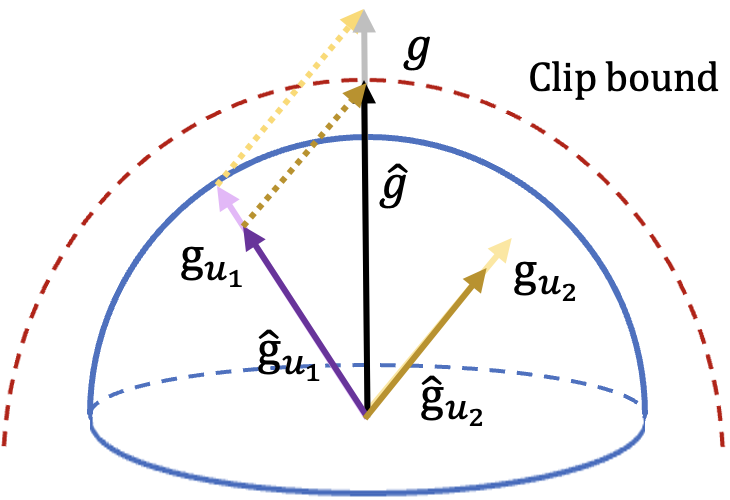
(a) clipping mechanism of DP-SGD

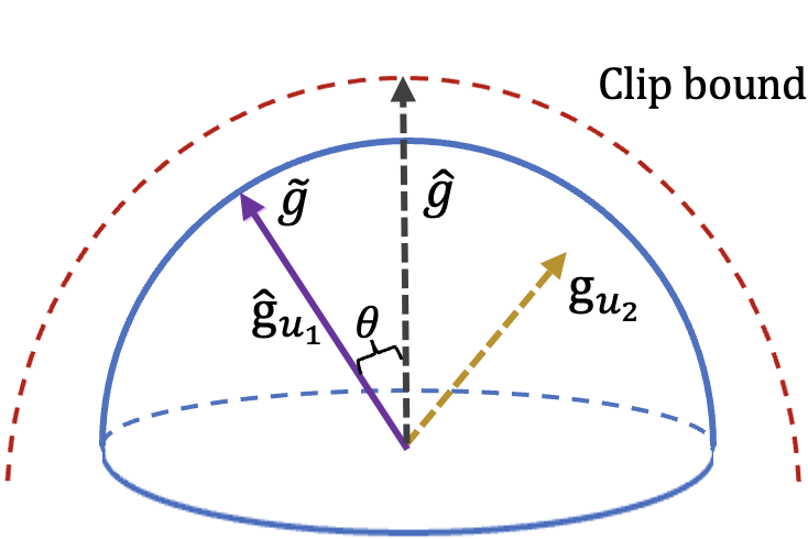
(b) clipping mechanism of PCDP-SGD

Figure 1: Schematic diagram of gradient clipping mechanism comparison. It can be observed that given the projection $V_{u_{1}}$, the projected per-sample gradient $\widetilde{g}=V_{u_{1}}V^{T}_{u_{1}}g=g_{u_{1}}$, that is, the top gradient component, is more preserved after clipping, relaxing the clipping bound and allowing the gradient to adapt to a smaller clipping threshold. Besides, we can see that the gradient direction may deviate by $\theta$, leading the gradient towards a more active descent direction. Here, $\hat{g}$ represents the clipped gradient.

2 Related Work

Compared to PDP-SGD The intensity of injected noise for achieving DP scales linearly with the model parameters $d$, which results in a high-dimension curse and ruins the convergence of DP-SGD. To solve it, PDP-SGD proposed by Zhou et al. [43] generally minimize the private empirical risk from the dependence factor $\sqrt{d}$ down to $\sqrt{k}$ by projecting the private gradient of sensitive data into a low-rank public subspace, and compensate the uniform bound of public projection reconstruction error with $\log{d}$ through the generic chaining [38]. However, PDP-SGD has a fatal oversight, as they did not consider gradient clipping in algorithm design and theory, which is crucial for DP-SGD. In addition, the attenuating effect of the projection on the gradient $l_{2}$ norm is also forgotten, which is sensitive to the clipping threshold. Admittedly, analyzing the convergence of DP-SGD with clipping functions is indeed challenging [41, 42, 11]. Compared to PDP-SGD, (1) our work based on the advanced clipping theory tools, establishes a set of DP-SGD theoretical analyses with pre-projection operation. (2) We demonstrate the effectiveness of our method in narrowing the clipping errors and bias. (3) As a complement to the uniform projection reconstruction bound in PDP-SGD, we flavor a projection reconstruction theory that independently segments public data.

Orthogonal to adaptive clipping To the best of our knowledge, there are works [4, 33] adaptively tune the appropriate clipping threshold in DP-SGD. Our work can be compatible with them and encourage them to adapt to smaller clipping thresholds. Also, automatic clipping (Auto-S) [9], normalized clipping (NSGD) [40] and per-sample adaptive clipping (DP-PSAC) [39] are proposed to optimize the clipping function. All of these normalized works are structurally different from Abadi’s clipping function, implicitly setting the clipping threshold to 1, thereby decoupling it from the learning rate. Our work is based on the form and theory of the classic Abadi’s clipping function, in which the clipping threshold and the learning rate are closely related. And our goal is to alleviate the impact of clipping errors and bias on the parameter adjustment and model utility as much as possible.

Federated learning with data heterogeneity and differential privacy. Local drifts with non-IID data distribution are mainly current obstacles in both FL and DPFL. The local non-IID data distribution could shift the client gradients to a more dispersed direction. To alleviate this unfavorable situation, FedProx [24] directly limits the $l_{2}$ norm of the gap between the local model and the global model to control the magnitude of local client offset. MOON [23] involves contrastive loss to correct the updated local gradient, which widens the distance between current local model features and historical features, and tightens the distance between current local model features and global features. Similarly, as a pre-clipping method, Cheng et al. [12] utilizes bounded regularization to constrain the $l_{2}$ norm of updates before local clipping in client-level DPFL. Other orthogonal efforts are trying to improve the utility of DPFL by limiting the magnitude of local updates [35] and sparsification [18] after clipping. Moreover, there is no specific work on non-IID data distribution under DPFL.

3 Preliminaries

As a general framework for differentially private optimization, our method considers both centralized and federated settings. So we introduce the privacy definition and both settings formally in this section. In addition, we follow existing assumptions [45, 28] as shown in Appendix A.2.

Definition 1 (Differential Privacy).

A randomized algorithm $M$ is $(\epsilon,\delta)$-differentially private if for any two neighboring datasets $D$, $D^{\prime}$ differ in exactly one data point, and for any event $Y$, we have

$$P(M(D)\in Y)\leq e^{\epsilon}P(M(D^{\prime})\in Y)+\delta.$$ (1)

Centralized Scenario: Given a private dataset $\mathcal{D}$, containing $|\mathcal{D}|$ pieces of data drawn i.i.d. from the underlying distribution $\mathcal{P}$, the differentially private empirical risk minimization goal is to minimize $\mathcal{L}(w)=\sum_{i=1}^{|\mathcal{D}|}\mathcal{l}(w,x_{i})$, where the parameter $w\in\mathbb{R}^{d}$. We define per-sample gradient $\nabla\mathcal{l}(w_{t},x_{i})=\nabla\mathcal{L}(w_{t})+\eta_{t,i}$ where $\eta_{t,i}$ is zero mean gradient noise and $\nabla\mathcal{L}(w_{t})=E_{x_{i}\sim\mathcal{P}}[\nabla\mathcal{l}(w_{t},x_{i})]$. Additionally, the mini-batch gradient with batch size $B$ is represented as $g_{t}=\frac{1}{B}\sum_{i=1}^{B}\nabla\mathcal{l}(w_{t},x_{i})$.
We exploit a new convergence paradigm that more explicitly highlights the role of the clipping function, i.e., $\mathbb{E}_{\eta_{t}\sim\mathcal{P}}[\langle\nabla\mathcal{L}(w_{t}),g_{t,\eta_{t}}\rangle]=\mathbb{E}_{\eta^{\prime}_{t}\sim\mathcal{P^{\prime}}}[\langle\nabla\mathcal{L}(w_{t}),g_{t,\eta^{\prime}_{t}}\rangle]+b_{t}$, that is to seek a good distribution $\eta^{\prime}_{t}\sim\mathcal{P^{\prime}}$ satisfying the symmetric properties, i.e., $\mathcal{P^{\prime}}(\eta^{\prime}_{t})=\mathcal{P^{\prime}}(-\eta^{\prime}_{t})$ to approximate the original distribution $\mathcal{P}$. Besides, we also pay attention to the clipping bias $b_{t}=\int\langle\nabla\mathcal{L}(w_{t}),g_{t,\eta_{t}}\rangle\mathcal{P}(\eta_{t})d\eta_{t}-\int\langle\nabla\mathcal{L}(w_{t}),g_{t,\eta^{\prime}_{t}}\rangle\mathcal{P^{\prime}}(\eta_{t}^{\prime})d\eta_{t}^{\prime}$ below.
Eigenspace: Considering a publicly available auxiliary dataset $\mathcal{D}_{pub}$, we use $\mathcal{S}_{t}$ to denote the second moment of the public mini-batch gradient, i.e., $\mathcal{S}_{t}=\sum_{i=1}^{B}\nabla\mathcal{l}(w_{t},x^{pub}_{i})\nabla\mathcal{l}(w_{t},x^{pub}_{i})^{T}$ with public sampling data $x^{pub}$ and use $H_{t}$ to denote the expectation of the public gradient population second moment from the sampling distribution $\mathcal{P}$, i.e., $H_{t}=E_{x^{pub}\sim\mathcal{P}}[\nabla\mathcal{l}(w_{t},x^{pub})\nabla\mathcal{l}(w_{t},x^{pub})^{T}]$. Let $V_{t}V_{t}^{T}$ denote the whole projection eigenspace of $\mathcal{S}_{t}$, and $V_{t,k}V_{t,k}^{T}$ denote the top-$k$ eigenspace.
Federated Scenario: Given global parameters $w_{g}$ and client data $\mathcal{D}_{c}\subseteq\mathcal{D}$, federated learning aims to solve an optimization problem: $\min_{w_{g}\in\mathbb{R}^{d}}\mathcal{L}(w_{g})=\frac{1}{N}\sum_{i\in N}(\mathcal{L}_{i}(w_{l},\mathcal{D}_{c}):=E_{\mathcal{D}_{c}\sim\mathcal{P}_{i}}[\mathcal{l}_{i}(w_{l},\mathcal{D}_{c})])$, where the local optimization solve of $i$-th client $\mathcal{L}_{i}(w_{l},\mathcal{D}_{c})$ is the expectation of the local loss function $\mathcal{l}_{i}(w_{l},\mathcal{D}_{c})$ with the local model parameters $w_{l}$. The data distribution $\mathcal{P_{i}}$ could vary hugely between clients under non-IID conditions. The notations concerning the eigenspace will follow that of the centralized scene.

4 Projected Clipping Differentially Private Gradient Descent

Algorithm 1 PCDP-SGD: Projected Clipping Differentially Private Gradient Descent

Input: Epoch $E$, total train samples $|\mathcal{D}|$, private batch size $B$, public batch size $B^{pub}$, iteration $T$, noise scale $\sigma$, clipping threshold $c$, learning rate $\gamma$ and projection dimension $k$.

1:  Initialize $w_{0}$ randomly and state the public dataset segmentation strategy.

2:  for $e\in E$ do

3:     Initialize $V_{t,k}$ to None.

4:     for $t\in T$ do

5:        Take a random Batch $B$ from private dataset with sampling probability $B/|\mathcal{D}|$.

6:        $g_{t}(x_{i})=\nabla\mathcal{l}(w_{t},x_{i})$.

7:        Compute public-based top-$k$ eigenvector $V_{t,k}$ of $\sum_{j\in B^{pub}}\nabla\mathcal{l}(w_{t},x^{pub}_{j})\nabla\mathcal{l}(w_{t},x^{pub}_{j})^{T}$.

8:        Projection on individual private gradient

9:        $\hat{g}_{t}(x_{i})=V_{t,k}V^{T}_{t,k}g_{t}(x_{i})$ .

10:        Clip per-sample projected gradient

11:        $\overline{g}_{t}(x_{i})=\hat{g}_{t}(x_{i})/max(1,\frac{\|\hat{g}_{t}(x_{i})\|_{2}}{c})$ .

12:        Add noise and average

13:        $\widetilde{g}_{t}=\frac{1}{B}\left(\sum_{i\in B}\overline{g}_{t}(x_{i})+V_{t,k}V^{T}_{t,k}\mathbb{N}(0,c^{2}\sigma^{2}\mathbb{I})\right)$.

14:        Update

15:        $w_{t+1}=w_{t}-\gamma\widetilde{g}_{t}$.

16:     end for

17:  end for

4.1 PCDP-SGD Framework

As a variant of noisy gradient descent, Algorithm 1 outlines our PCDP-SGD method for minimizing the private empirical loss function $\mathcal{L}(w)$. At every step $t$, we sample random gradients $\nabla\mathcal{l}(w_{t},x_{i})$, get projection by computing top-$k$ eigenvector with public gradients $\nabla\mathcal{l}(w_{t},x^{pub}_{j})$, project individual private gradient $g_{t}(x_{i})$, clip each gradient with the $l_{2}$ norm threshold $c$ and add isotropic Gaussian noise to the gradient. Compared with DP-SGD and PDP-SGD, we highlight the projected gradient $V_{t,k}V^{T}_{t,k}g_{t}(x_{i})$ before the clipping operation (line 9 in Algorithm 1). In this section, we will analyze the properties of PCDP-SGD in centralized settings from privacy guarantee, projection reconstruction error, convergence analysis of pre-projection on clipping bias, and clipping bias correction.

4.2 Privacy Guarantee

PCDP-SGD is designed to project the per-sample gradient $g_{t}(x_{i})$ before clipping as shown in Eq. 2,

$$\overline{g}_{t}(x_{i})=V_{t,k}V^{T}_{t,k}g_{t}(x_{i})/max(1,\frac{\|V_{t,k}V^{T}_{t,k}g_{t}(x_{i})\|_{2}}{c})\vspace{-0.1cm}$$ (2)

and utilizes the projected clipped noisy gradient $\widetilde{g}_{t}(x_{i})=\frac{1}{B}\left(\sum_{i\in B}\overline{g}_{t}(x_{i})+V_{t,k}V^{T}_{t,k}\mathbb{N}(0,c^{2}\sigma^{2}\mathbb{I})\right)$ to update parameters. Despite the projection being assisted by public information, it does not compromise privacy [3, 5]. Here, we explicitly state the privacy guarantee of PCDP-SGD.

Theorem 1 (Privacy).

Under the assumption A.1, there exist constants $m_{1}$ and $m_{2}$ such that for any $\epsilon\leq m_{1}q^{2}T$, $\delta>0$ and $\sigma^{2}_{dp}=m_{2}\frac{Tc^{2}q^{2}\ln{\frac{1}{\delta}}}{\epsilon^{2}}$ over the $T$ iterations, where $q=\frac{B}{|\mathcal{D}|}$, PCDP-SGD is $(\epsilon,\delta)$-differentially private.

Since pre-projection itself does not involve privacy, the per-sample gradient is still bounded by the clipping threshold. Therefore, the privacy proof follows the proof in [1]. Then, based on the post-processing property, releasing the gradient $\widetilde{g}_{t}(x_{i})$ satisfies differential privacy.

4.3 Projection Reconstruction Error

Generating the projection based on public auxiliary samples is not lossless. To be exact, since the projection subspace $V_{t,k}V_{t,k}^{T}$ generated from the sample second moment $\mathcal{S}_{t}$ approximates the population projection subspace $\widetilde{V}_{t,k}\widetilde{V}^{T}_{t,k}$ of the population second moment $H_{t}$, the projection subspace skewing $\|V_{t,k}V_{t,k}^{T}-\widetilde{V}_{t,k}\widetilde{V}^{T}_{t,k}\|_{2}$ can not be neglected. Different auxiliary data segmentation methods have distinct projection effects in experiments and theory. Non-independent segmentation [43] means that each round randomly extracts batch samples from the auxiliary dataset, but it causes data reuse and model parameter dependence. However, independent partitioning can avoid this situation, referring to randomly dividing the auxiliary public dataset with size $m$ into the non-overlapping small blocks with size $\frac{m}{T}$ according to the iteration rounds $T$. We supplement the intuitive independent projection reconstruction error:

Theorem 2 (Subspace Skewing under Independent Segmentation).

Under Assumption A.1 and A.2, $\lambda_{k}(\mathcal{S}_{t})$ denotes the $k$-th eigenvalue of the matrix $\mathcal{S}_{t}$ and $\Delta_{k}(\mathcal{S}_{t})$ denotes the eigen-gap in the $t$-th iteration such that $\Delta_{k}(\mathcal{S}_{t}):=\lambda_{k}(\mathcal{S}_{t})-\lambda_{k+1}(\mathcal{S}_{t})\geq\|\mathcal{S}_{t}-H_{t}\|_{2}$, for $\forall t\in T$, when $\Delta_{k}(\mathcal{S}_{t})\geq\mathcal{O}(\frac{G^{2}\sqrt{T\log{d}}}{\sqrt{m}})$, the upper bound of subspace skewing $\Lambda_{t}:=\mathbb{E}[\|V_{t,k}V_{t,k}^{T}-\widetilde{V}_{t,k}\widetilde{V}_{t,k}^{T}\|_{2}]$ satisfies:

$$\Lambda_{t}\leq\mathcal{O}(\frac{\sqrt{T}G^{2}\sqrt{\log{d}}}{\Delta_{k}\sqrt{m}}).$$

Based on Theorem 2, we can bound the reconstruction gap with the factor $\log{d}$ between the empirical projection $V_{t,k}V_{t,k}^{T}$ and the true projection $\widetilde{V}_{t,k}\widetilde{V}_{t,k}^{T}$, which is also related to the eigen-gap $\Delta_{k}$ of the sampling gradient. The selection of $k$ will have an impact on the reconstruction error, as shown in Appendix G.2.
Then, we analyze the distribution deviation caused by the assumption of symmetry distribution with regard to gradient clipping. Due to the disparity between the population second moment of gradient $Z_{t}=\mathbb{E}_{\eta^{\prime}_{t}\sim\mathcal{P}^{\prime}}[(\nabla\mathcal{L}(w_{t})+\eta^{\prime}_{t})(\nabla\mathcal{L}(w_{t})+\eta^{\prime}_{t})^{T}]$ that follows the symmetric distribution and the population second moment of gradient $H_{t}=\mathbb{E}_{\eta_{t}\sim\mathcal{P}}[(\nabla\mathcal{L}(w_{t})+\eta_{t})(\nabla\mathcal{L}(w_{t})+\eta_{t})^{T}]$ that follows the original distribution, the projection $V_{t,k}V_{t,k}^{T}$ generated by the original gradient theoretically introduces additional reconstruction errors. We need to bound the gap between the two population second moments, i.e., $\|H_{t}-Z_{t}\|_{2}$.

Corollary 1 (Subspace Skewing with Distribution Deviation).

Let $\nabla\mathcal{L}(w_{t})=\mathbb{E}[\nabla\mathcal{l}(w_{t},x)]$ and $\nabla\mathcal{l}(w_{t},x)=\nabla\mathcal{L}(w_{t})+\eta_{t}$, $\eta_{t}\sim\mathcal{P}$ is the sampling noise with zero mean and eigen cumulative variance $\sum^{d}_{i=1}\sigma^{2}_{\eta,i}$. Correspondingly, suppose there is a zero-mean symmetric distribution $\eta^{\prime}_{t}\sim\mathcal{P^{\prime}}$ with the variance $\sum^{d}_{i=1}\sigma^{2}_{\eta^{\prime},i}$, such that $\nabla\mathcal{l}^{\prime}(w_{t},x)=\nabla\mathcal{L}(w_{t})+\eta^{\prime}_{t}$ and $\mathbb{E}[\nabla\mathcal{l}^{\prime}(w_{t},x)]=\nabla\mathcal{L}(w_{t})$, when $\Delta_{k}(\mathcal{S}_{t})\geq\mathbb{E}[\|\mathcal{S}_{t}-H_{t}\|_{2}]+\sigma^{2}_{*}$, we have

$$\overline{\Lambda}_{t}:=\mathbb{E}[\|V_{t,k}V_{t,k}^{T}-V^{\prime}_{t,k}V^{\prime T}_{t,k}\|_{2}]\leq\Lambda_{t}+\mathcal{O}(\frac{\sigma^{2}_{*}}{\Delta_{k}}),$$

where $\sigma^{2}_{*}=\max_{i}(\sigma^{2}_{\eta,i}-\sigma^{2}_{\eta^{\prime},i})$ is the maximum eigen-gap between the covariance of $\eta$ and $\eta^{\prime}$.

In Corollary 1, it can be seen that the gap between $H_{t}$ and $Z_{t}$ comes from the maximum variance component of the two noise distributions. When the original distribution $\mathcal{P}$ is approximately symmetric, the deviation $\sigma^{2}_{*}$ becomes small. Meanwhile, due to $\mathcal{P}$ empirically covers a finite sample, the gap is always a trivial constant factor [11].

4.4 DP-SGD Convergence with Pre-projection

In this section, we investigate the convergence of PCDP-SGD under the non-convex condition. We consider that when the clipping threshold is large enough, the clipping operation does not change the per-sample gradient. Therefore, the position of projection is irrelevant. We first study the convergence without clipping bias in this case, laying the groundwork for the convergence with clipping bias.

Theorem 3 (PCDP-SGD without Clipping Bias).

Under assumption A.1 and A.2 with $\rho$-smooth loss function $\nabla\mathcal{L}(w_{t})$, as $c\to G$, for the projected clipping DP-SGD with the sampling possibility $q=B/|\mathcal{D}|$, if we set $\gamma=\frac{\sqrt{D_{\mathcal{L}}d\ln{\frac{1}{\delta}}}}{|\mathcal{D}|\epsilon G\sqrt{\rho}}$ and $\Lambda^{*}=\frac{1}{T}\sum_{t=1}^{T}\Lambda^{2}_{t}$, there exist constants $m_{1}$ and $m_{2}$ such that for any $\epsilon\leq m_{1}q^{2}T$ and $\sigma^{2}_{dp}=m_{2}\frac{Tc^{2}q^{2}\ln{\frac{1}{\delta}}}{\epsilon^{2}}$ over the $T$ iteration, we achieve

$$\frac{1}{T}\sum_{t=1}^{T}\|\nabla\mathcal{L}(w_{t})\|_{2}^{2}\leq\mathcal{O}(\frac{qG\sqrt{\rho k}}{\epsilon})+\Lambda^{*}.$$

From Theorem 3 above, projection can reduce the privacy budget $\epsilon$ dependence of a factor of $\sqrt{d}$ to $\sqrt{k}$ and it can be seen that if the clipping threshold is large enough, the overall convergence bound is related to the upper bound of gradient $G$, which may harm convergence rate. Under the circumstances, we turn the spotlight on the PCDP-SGD with the small clipping threshold region, where the clipping function will work.

Theorem 4 (PCDP-SGD with Clipping Bias).

Under assumption A.1, A.2 and A.3, as $c<G$, for the $\rho$-smooth loss function $\mathcal{L}(w_{t})$, if we choose the symmetric distribution $\mathcal{P^{\prime}}$ with variance $\sum^{d}_{i=1}\sigma^{2}_{\eta^{\prime},i}$, i.e., $\eta^{\prime}_{t}\sim\mathcal{P^{\prime}}$ and $\mathcal{P^{\prime}}(\eta^{\prime}_{t})=\mathcal{P^{\prime}}(-\eta^{\prime}_{t})$, let $\gamma=\frac{\sqrt{D_{\mathcal{L}}d\ln{\frac{1}{\delta}}}}{|\mathcal{D}|\epsilon c\sqrt{\rho}}$ and there exist constants $m_{1}$ and $m_{2}$ such that for any $\epsilon\leq m_{1}q^{2}T$ and $\sigma^{2}_{dp}=m_{2}\frac{Tc^{2}q^{2}\ln{\frac{1}{\delta}}}{\epsilon^{2}}$ over the $T$ iteration, PCDP-SGD achieves:

$\forall\tau\in(0,1)$, if $\|\Pi^{+}_{V_{t,k}}\nabla\mathcal{L}(w_{t})\|_{2}\leq(1-\tau)c$, with $\overline{\Lambda}^{*}=\frac{1}{T}\sum_{t=1}^{T}\overline{\Lambda}^{2}_{t}$ and $\Psi:=\frac{1}{T}\sum_{t=1}^{T}\|\nabla\mathcal{L}(w_{t})\|_{2}^{2}$,

$$\Psi \leq\underbrace{\mathcal{O}(\frac{(1-\tau)^{2}c\sqrt{\widetilde{\sigma}}}{\tau})}_{\text{clipping error term}}+\mathcal{O}({\frac{cB\sqrt{\rho k}}{|\mathcal{D}|\epsilon}})+\underbrace{\mathcal{O}(Gc\overline{b}_{t})}_{\text{clipping bias term}}+\overline{\Lambda}^{*},$$

and if $\|\Pi^{+}_{V_{t,k}}\nabla\mathcal{L}(w_{t})\|_{2}\geq(1-\tau)c$, with $\overline{\Lambda}^{*}=\frac{1}{T}\sum_{t=1}^{T}\overline{\Lambda}_{t}$ and $\Psi^{*}:=\frac{1}{T}\sum_{t=1}^{T}\|\nabla\mathcal{L}(w_{t})\|_{2}$,

$$\Psi^{*} \leq\underbrace{\mathcal{O}(\frac{(1-\tau)\sqrt{\widetilde{\sigma}}}{\tau})}_{\text{clipping error term}}+\mathcal{O}(\frac{B\sqrt{\rho k}}{(1-\tau)|\mathcal{D}|\epsilon})+\underbrace{\mathcal{O}(\frac{G\overline{b}_{t}}{1-\tau})}_{\text{clipping bias term}}+\overline{\Lambda}^{*},$$

where $\widetilde{\sigma}=\sum^{k}_{i=1}\sigma^{2}_{\eta^{\prime},i}$ denotes top-$k$ variance branches and $\overline{b}_{t}=\frac{1}{T}\sum_{t=1}^{T}\int_{\eta_{t}}|\mathcal{P}(\eta_{t})-\mathcal{P^{\prime}}(\eta_{t}^{\prime})|d\eta_{t}$ is the clipping bias over the $T$ iterations.

Theorem 4 shows that PCDP-SGD reduces the clipping error term from the factor $\sum^{d}_{i=1}\sigma^{2}_{\eta^{\prime},i}$ to $\sum^{k}_{i=1}\sigma^{2}_{\eta^{\prime},i}$. Since a nice and ideal distribution $\mathcal{P}^{\prime}$ could be more concentrated and symmetrical than the actual distribution $\mathcal{P}$, the partial variance $\widetilde{\sigma}$ of $\mathcal{P}^{\prime}$ should be bound by a constant $G$. Specifically, if we relax the definition of this nice distribution and basically regard it as an isotropic Gaussian noise according to the Central Limit Theorem [19, 28], then the term will be reduced from the factor $\sqrt{d}$ to the factor $\sqrt{k}$, despite the existence of more sophisticated assumptions [36, 45].
No need to tune clipping threshold in PCDP-SGD We present a remarkable discovery in Theorem 4: when the projected population gradient consistently remains below the clipping threshold $c$, the convergence bound in PCDP-SGD with Abadi’s clipping can be independent of the clipping threshold. By incorporating pre-projection, we have effectively decreased the gradient norm of individual samples, expanding the scope for a small clipping threshold condition. The conclusions derived from prior work [9] on adaptive clipping should be more accurately established within the context of a small $c$ region. To underscore this point, we will reevaluate and validate this conclusion in the experiments.

4.5 Clipping Bias Correction

The clipping bias term essentially implies the gap between the true distribution and a symmetric distribution. Subsequently, we experimentally and theoretically characterize and compare the distributions before and after projection through the standard noise correction. In experiments, we extract the partial layers by reducing the gradient dimension to two dimensions through random matrices. Theoretically, we analyze the noise correction quantity required for transforming the projected distribution into a symmetric distribution.
From Fig. 6, we obtain that the gradient distribution by projection (pink points) presents more locally symmetrical and concentrated than the previous one (blue points).

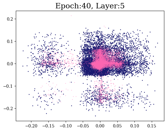
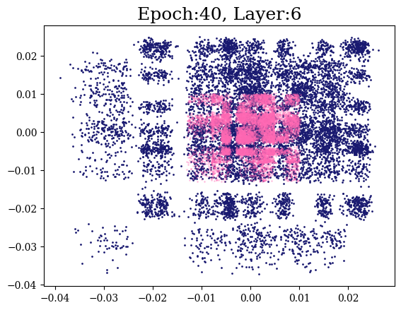
Figure 2: Gradient distributions with/without projection under the setting of $c=0.01$ and $\gamma$ = 1. The experiment is conducted on the CIFAR10 dataset with LeNet network.

Theorem 5 (Clipping Bias Correction).

Assuming that there is a symmetric distribution $\omega\zeta_{t}\sim\widetilde{\mathcal{P}}$ can minimize the gap between the projected distribution $\mathcal{P}$. Let corrected gradient $\widetilde{g}_{t,\eta_{t}\sim\mathcal{P}}=clip(\Pi_{V_{t,k}}^{+}(\nabla\mathcal{L}(w_{t})+\eta_{t})+\omega\zeta_{t})$, $\Pi_{V_{t,k}}^{+}=V_{t,k}V_{t,k}^{T}$ and $\zeta\sim\mathbb{N}(0,\mathbb{I}_{d})$. Then the term of clipping bias $b_{t}$ in the original convergence bound can be further described as

$$\min\{\|\Pi_{V_{t,k}}^{+}\nabla\mathcal{L}(w_{t})\|_{2},(1-\tau)c\}\|\nabla\mathcal{L}(w_{t})\|_{2}\mathbb{P}(\|\omega\zeta_{t}\|_{2}<\tau c)$$

$$-\mathcal{O}(\frac{\hat{\sigma}}{\omega^{2}})\leq\mathbb{E}_{\eta_{t}\sim\mathcal{P},\omega\zeta\sim\mathcal{\widetilde{P}}}[\langle\nabla\mathcal{L}(w_{t}),\widetilde{g}_{t}\rangle],$$

where $\hat{\sigma}=\sum^{k}_{i=1}\sigma^{2}_{\eta,i}$ is the sum of top-$k$ eigenvalues of the gradient noise covariance $\eta_{t}$ and $\omega$ is a variance amplitude constant.

In the light of Theorem 5, compared to the conclusion with a factor of $\sum^{d}_{i=1}\sigma^{2}_{\eta,i}$ in Chen et al. [11], our method requires a smaller $\omega$, namely, a correction perturbation distribution with smaller variance, to offset the clipping bias term. In other words, it can be seen that the projected distribution could be more symmetric and concentrated.

Table 1: Test accuracy and standard deviation on vision tasks of PCDP-SGD in the centralized scenario over 4 runs.

Dataset	MNIST-Accuracy %				FMNIST-Accuracy %
Method	Privacy budget $\epsilon$ / Noise multiplier $\sigma$				Privacy budget $\epsilon$ / Noise multiplier $\sigma$
	0.69 / 10	0.49 / 14	0.38 / 18	0.31 / 22	1.18 / 6	0.49 / 14	0.31 / 22	0.23 / 30
DP-SGD	87.85$\pm$1.61	79.39$\pm$2.09	66.09$\pm$1.62	50.51$\pm$3.16	74.49$\pm$0.65	70.43$\pm$0.23	63.24$\pm$0.33	48.74$\pm$3.19
PDP-SGD	88.24$\pm$0.49	87.00$\pm$1.24	84.74$\pm$0.89	83.59$\pm$0.45	71.96$\pm$0.62	70.87$\pm$0.35	69.54$\pm$0.61	66.21$\pm$1.70
RPDP-SGD	87.40$\pm$0.78	85.25$\pm$0.85	82.71$\pm$0.68	78.06$\pm$0.67	70.57$\pm$0.37	70.43$\pm$0.34	67.83$\pm$0.69	63.86$\pm$0.32
RSDP-SGD	86.79$\pm$0.96	76.86$\pm$0.71	62.39$\pm$1.73	49.44$\pm$1.43	72.96$\pm$0.28	69.87$\pm$0.49	60.40$\pm$0.95	45.52$\pm$3.63
PCDP-SGD	88.51$\pm$0.57	87.99$\pm$0.83	86.10$\pm$0.93	85.20$\pm$0.49	72.21$\pm$0.63	71.28$\pm$0.41	70.06$\pm$0.53	68.18$\pm$0.94

5 PCDP-SGD for Federated Learning

5.1 FedPCDP Framework

Algorithm 2 FedPCDP: Federated PCDP-SGD in Subspace

Server Input: Global parameters $w_{g}$, global learning rate
$\gamma_{g}$, client count $N$, client sample ratio $S/N$, projection dimension $k$ and communication round $R$.
Client Input: local parameters $w_{l}$, local learning rate $\gamma_{l}$, and local steps $T$.

1:  Initialize $w^{0}_{g}$ randomly.

2:  for each communication $r\in R$ do

3:     Select clients with $S/N$ randomly.

4:     Allocate $w^{r-1}_{g}$ to the participants.

5:     Call VirtualClientProcedure($w^{r-1}_{g}$,$\mathcal{D}^{pub}$,$r$,$k$) (Algorithm 3) and obtain the projection $V^{r}_{k}$.

6:     Share $V^{r}_{k}$ with the participants.

7:     Client $i\in S$ in parallel:

8:     Initialize local model $w_{l,0}^{i}=w^{r-1}_{g}$.

9:     for each local step $t\in T$ do

10:        Run PCDP-SGD (Algorithm 1) excluding line 7.

11:     end for

12:     Compute $\nabla w^{i}=w^{r-1}_{g}-w^{i}_{l,T-1}=\sum^{T-1}_{t=0}\widetilde{g}(w^{i}_{l,t})$.

13:     Upload $\nabla g^{i}=V^{rT}_{k}\nabla w^{i}$ to the sever.

14:     end on clients

15:     Restore the gradient and update global parameters:

16:     $w^{r}_{g}=w^{r-1}_{g}-\gamma_{g}\frac{1}{|S|}\sum_{i\in S}V^{r}_{k}\nabla g^{i}$.

17:  end for

Considering the lack of specific methods for handling data heterogeneity in privacy-preserving federated learning, as a supplementary and evolving approach, we incorporate PCDP-SGD into the FL framework. Overall, the steps of PCDP-SGD framework in DPFL named FedPCDP (Algorithm 2) are as follows: (1) set up a virtual client with publicly available auxiliary data $\mathcal{D^{pub}}$ to generate a one-round $r$ general projection matrix $V^{r}_{k}$. (2) the chosen clients $S$ use the transposition of public projection $V^{r}_{k}$ to compress the local gradient $\nabla w^{i}$ and obtain the gradient $\nabla g^{i}$ for communication. (3) the server restores the gradient $\nabla g^{i}$ through $V^{r}_{k}$ and update the global model parameters.

Algorithm 3 Function: VirtualClientProcedure($\cdot$)

Input: Global parameters $w_{g}$, projection dimension $k$, current round $r$ and auxiliary dataset $\mathcal{D}^{pub}$.

1:  Virtual client parameters $w_{v}=w^{r-1}_{g}$.

2:  for $t\in T$ do

3:     Sample batch $B^{pub}\subseteq\mathcal{D}^{pub}$.

4:     Calculate gradients $g_{t}(x^{pub}_{i})=\nabla\mathcal{l}(w_{v},x^{pub}_{i})$.

5:     if $t==T$ then

6:        Generate public projection $V^{r}_{k}$ by computing $\sum_{j\in B^{pub}}\nabla\mathcal{l}(w_{v},x^{pub}_{j})\nabla\mathcal{l}(w_{v},x^{pub}_{j})^{T}$.

7:     end if

8:  end for

9:  return $V^{r}_{k}$

5.2 Convergence of Federated PCDP-SGD

We study the convergence of PCDP-SGD in federated scenarios. After private clients complete $T$ local steps, the server randomly selects $S$ clients without replacement. The selected clients sent the reduced gradient to the server, and the gradient will be restored and aggregated in the center. Extracting the clipping term, we provide the convergence of federated PCDP-SGD:

Theorem 6 (Federated PCDP-SGD in Subspace).

Under Assumption A.1, A.2, and A.4, let $\Lambda^{*}=\frac{1}{T}\sum_{t=1}^{T}\Lambda_{t}$ denote projection reconstruction error and $T=\sqrt{\frac{S}{\overline{c}^{r}}}$, on the condition of $\gamma_{l}\leq\frac{1}{2\rho\overline{c}^{r}T}$, $\gamma^{2}_{l}\leq\frac{1}{216T^{2}\rho^{2}(\overline{c}^{r})^{2}}$ and $\gamma_{g}\gamma_{l}\leq\min(\frac{1}{36\rho^{g}},\frac{1}{648(\overline{c}^{r})^{3}\rho^{g}})$, the exist constant $\kappa>0$, and FedPCDP achieves:

$$\frac{\kappa}{R}\sum^{R}_{r=1}E[\overline{c}^{r}\|\nabla\mathcal{L}(w^{r}_{g})\|^{2}]\leq\frac{24\mathcal{L}^{*}}{\gamma_{g}\gamma_{l}R}+\frac{G^{2}}{RS}\sum_{r,t,i}E[\mathcal{C}^{r2}_{i,t}+\widetilde{\mathcal{C}}^{r2}_{i,t}]$$

$$+\sum_{r,t,i}\frac{24G^{2}}{RN}E[|\mathcal{C}^{r}_{i,t}|+|\widetilde{\mathcal{C}}^{r}_{i,t}|]+\frac{G^{2}}{3RSN}E[\mathcal{C}^{r2}_{i,t}+\widetilde{\mathcal{C}}^{r2}_{i,t}]$$

$$+\frac{T}{9S}(21\widetilde{\sigma}_{l}+4k\sigma^{2}_{dp}+36T\widetilde{\sigma}_{g})+\frac{4(N-S)}{S(N-1)}\widetilde{\sigma}_{g}+2\Lambda^{*},$$

where $\mathcal{C}^{r}_{i,t}=c^{r}_{i,t-1}-\widetilde{c}^{r}_{i,t-1}$, $\widetilde{\mathcal{C}}^{r}_{i,t}=\widetilde{c}^{r}_{i,t-1}-\overline{c}^{r}$, $\widetilde{\sigma}_{l}=\sum^{k}_{i=1}\sigma^{2}_{l,i}$ and $\widetilde{\sigma}_{g}=\sum^{k}_{i=1}\sigma^{2}_{g,i}$.

From the convergence bound of FedPCDP with the clipping operation and sample-level DP guarantee, the dominant terms are the DP variance $\sigma^{2}_{dp}$ and cross-client variance $\Gamma^{f}_{g}$. The clipping bias term consists of $\mathcal{C}^{r}_{i,t}$ and $\widetilde{\mathcal{C}}^{r}_{i,t}$. $\mathcal{C}^{r}_{i,t}$. When $\Gamma^{f}_{l}$ is small, $\mathcal{C}^{r}_{i,t}$ could be negligible. And $\widetilde{\mathcal{C}}^{r}_{i,t}$ is related to the cross-client variance $\Gamma^{f}_{g}$, which is unavoidable [42]. For the DP term, projection can linearly scale $d$ to $k$ as in the central scenario. For the gap of local optimum across clients, there is an upper bound based on conventional assumptions, but due to projection, the boundary between the different local optimal points can be gathered closer, and its upper bound of $l_{2}$ norm could dwindle to the first $k$ components. We will verify these two points in experiments.

6 Experiments

6.1 Experimental Setup

We conduct experiments on centralized PCDP-SGD and federated PCDP-SGD with an Intel(R) Xeon(R) E5-2640 v4 CPU at 2.40GHz and a NVIDIA Tesla P40 GPU running on Ubuntu. We select three datasets: MNIST, Fashion-MNIST, and CIFAR10, and implement private SGD by BackPACK [13] in the convolutional neural network.
In the centralized scenario, we adopted an experimental setup similar to PDP-SGD [43], where we extract a subset of size 10,000 samples from the training set, making the training more challenging with fewer data. Additionally, we set the batch size $B=250$, clipping threshold $c=0.01$, learning rate $\gamma=1$, and run 80 epochs. Regarding the privacy composition theorems [1, 8], we fix $\delta=1e^{-5}$, set epsilon $\epsilon$ to $\{1.18,0.69,0.49,0.38,0.31,0.26,0.23\}$ for noise multiplier $\sigma\in\{6,10,14,18,22,26,30\}$ for MNIST and FMNIST. For CIFAR10, the epsilon $\epsilon$ is $\{4,1.8,1.18,0.69,0.49,0.38\}$ for noise multiplier $\sigma\in\{2,4,6,10,14,18\}$. For auxiliary information and projection settings, we randomly extract $m=100$ samples from the rest of the training set as a public dataset and set the projection dimension $k$ to 100 by default. Our baseline includes DP-SGD [1], PDP-SGD [43], RPDP-SGD using Random Projection [6] and RSDP-SGD with the dimension-wise pre-sparse method [44]. Although the adaptive clipping function is orthogonal to our work, we will still explore the compatibility of our approach with their methods [9, 40, 39].
In the federated scenario, we primarily validate the benefits of FedPCDP under the high-privacy regime. Similarly, we extract a subset of 50,000 samples from the training set, evenly distributed among $N=10$ clients. The remaining samples are used to create a public data pool with a size of $m=100$. We set the client sampling rate to 0.8 and conduct $R=80$ communication rounds. For the privacy budget, we set $\epsilon$ to $\{1.30,0.83,0,62,0.50\}$ for noise multiplier $\sigma\in\{4,6,8,10\}$. In particular, under the non-IID setting, we follow the method of McMahan et al. [29] to distribute the unbalanced data to local clients. It should be emphasized that in order to verify the theoretical field that projection can buffer the impact of cross-client variance, we set an extreme non-IID situation where each client contains predominantly only one class of data. Moreover, we utilized Pytorch to implement the mainstream FL methods targeting for non-IID: SCAFFOLD [21], FedProx [24], MOON [23] FedLRS [12] and simplified PFA [27] to conduct comparative experiments in the non-DP and DP conditions.
Due to space limitations, we place experiments on the coupling of clipping threshold and learning rate, projection frequency, public dataset segmentation, communication overhead, etc., in the Appendix.

Table 2: Test accuracy and standard deviation on vision tasks of FedPCDP in the federated scenario over 3 runs.

Dataset	MNIST-Accuracy %				FMNIST-Accuracy %
Method	Privacy budget $\epsilon$ / Noise multiplier $\sigma$				Privacy budget $\epsilon$ / Noise multiplier $\sigma$
	1.30 / 4	0.83 / 6	0.62 / 8	0.50 / 10	1.30 / 4	0.83 / 6	0.62 / 8	0.50 / 10
FedAvg [29]	84.70$\pm$0.79	63.95$\pm$4.52	37.45$\pm$4.79	26.66$\pm$2.63	72.33$\pm$0.61	66.80$\pm$0.74	56.46$\pm$2.13	43.17$\pm$3.82
FedProx	84.64$\pm$1.03	62.80$\pm$5.44	36.74$\pm$3.20	26.56$\pm$1.92	72.45$\pm$0.72	66.56$\pm$1.22	56.75$\pm$2.08	42.73$\pm$4.47
FedLRS	83.56$\pm$1.48	61.05$\pm$5.70	31.58$\pm$1.61	23.88$\pm$4.47	72.02$\pm$0.64	67.55$\pm$1.12	56.91$\pm$0.81	41.32$\pm$4.70
FedPDP	86.73$\pm$0.72	83.38$\pm$1.85	79.98$\pm$2.35	75.09$\pm$1.75	70.88$\pm$0.65	69.21$\pm$0.50	68.13$\pm$0.55	67.28$\pm$1.26
FedPCDP	88.96$\pm$1.38	87.21$\pm$1.72	85.58$\pm$0.86	83.65$\pm$2.83	71.10$\pm$0.46	70.23$\pm$0.55	68.59$\pm$0.66	69.08$\pm$0.66

6.2 Results of Centralized PCDP-SGD

6.2.1 Accuracy Comparison

Tab. 1 demonstrates that PCDP-SGD achieves the highest accuracy in the centralized settings under strong DP guarantee (small $\epsilon$ regime) on multiple datasets. In a relatively high-privacy (more rigorous) region, compared to DP-SGD, PCDP-SGD adopts projection which bypasses the ambient dimension and reduces noise scale caused by the high-dimensional curse. Compared to PDP-SGD, PCDP-SGD operates projection in advance, which mitigates the negative impact of clipping and data sampling on the gradient noise by decreasing the clipping bias term. In addition, PCDP-SGD outperforms RPDP-SGD due to its high-quality projection reconstruction, and the failure of RSDP-SGD is attributed to its dimension selection relying solely on randomness. The complete experiments and CIFAR-10 results are presented in the Appendix.

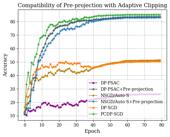
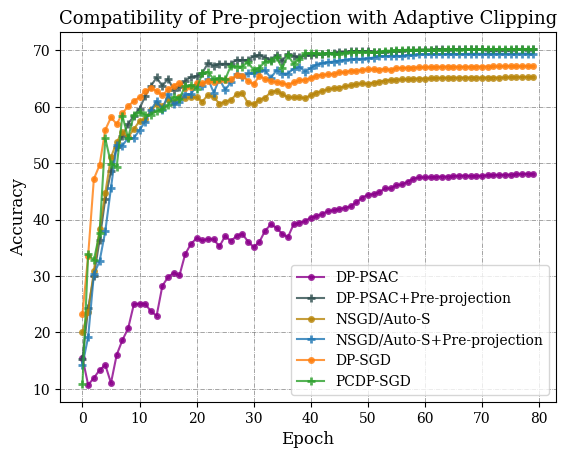
Figure 3: Accuracy($\%$) in the ablation experiments of pre-projection with adaptive clipping over 4 runs. Left: MNIST, $\epsilon=0.31$. Right: FMNIST, $\epsilon=0.38$. DP-PSAC: $r=0.0001$. NSGD/Auto-S: $r=0.01$

6.2.2 Compatibility Analysis with Adaptive Clipping

As shown in Fig. 3, we use the same learning rate $\gamma$ in the high-privacy regime. For adaptive clipping, similar to DP-SGD, it struggles to perform well (accuracy fluctuates around 50$\%$), and the algorithm becomes more sensitive to the choice of hyperparameter $r$ due to the larger added noise that disrupts the original $l_{2}$ norm landscape. In this scenario, similar to the gains observed in DP-SGD, pre-projection significantly enhances the utility of adaptive clipping. Additionally, we find that pre-projection narrows the gap between different variants of clipping functions. This is because the projection reduces the $l_{2}$ norm of gradients, making small gradients equally important and exploring the potential of gradients under the same clipping threshold.

6.3 Results of Federated PCDP-SGD

6.3.1 Accuracy Comparison

It can be seen from Tab. 2 that FedPCDP performs better than prevalent DPFL methods in the IID setting, and the benefits of projection in advance are consistent and prominent in federated scenarios. In the high-privacy regime, existing federated learning algorithms have not shown the capability to handle more severe levels of noise. Our approach, however, succeeds in mitigating the magnitude of noise within individual clients and preventing the cumulative negative impact on the federated model during aggregation by bypassing marginal dimensions to relieve DP noise.

6.3.2 Non-IID Alleviation

Continuing, we explore the impact of projection under extreme non-IID conditions in Fig. 4. Specifically, each client only holds one category of data as much as possible to maximize the cross-client variance $\Gamma^{f}_{g}$. Compared with current non-IID methods, our FedPCDP achieves better accuracy on both DP and non-DP settings. Though some method performs well in non-DP settings (like MOON), all the mainstream methods fail in DP settings.

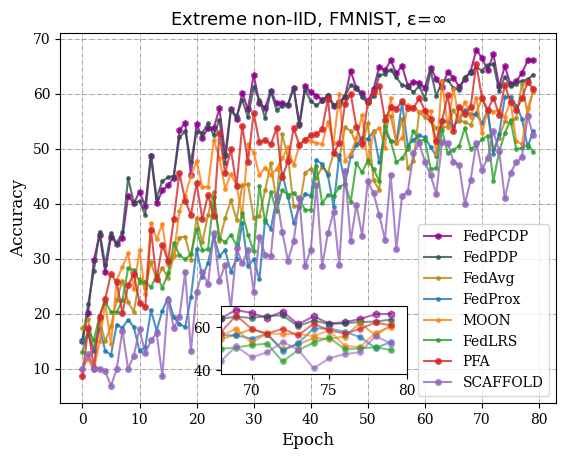
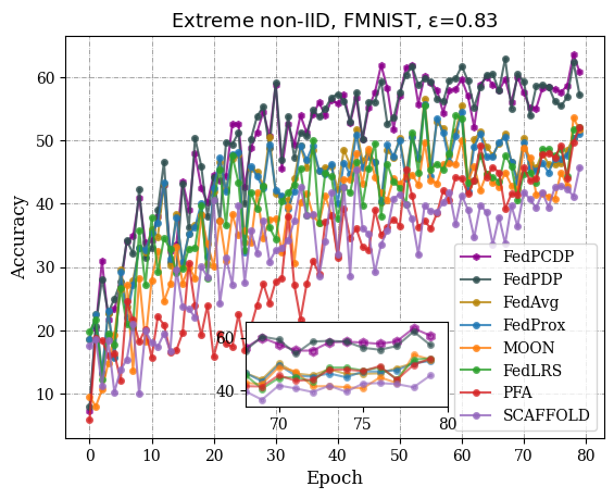
Figure 4: Performance in extreme non-IID over 3 runs.

The reason is that these mainstream methods more or less use historical or global gradients for correction and compensation. Regrettably, the auxiliary information contains DP noise, making the corrected gradient likely biased toward worse results.

7 Conclusion

The significance of gradient clipping in DP-SGD is garnering increased attention. The conventional clipping operation scales each dimension of the gradient uniformly, which may exacerbate the loss of crucial gradient information. To address this concern, we present the PCDP-SGD framework, which introduces pre-projection as a means to preserve more valuable top gradient components. In a centralized scenario, we explore an independent public dataset segmentation approach for additional projection reconstruction errors. Then, we analyze the optimization of gradient clipping introduced by projection and derive a theory for clipping bias correction. In a federated context, we leverage projection to curb cross-client divergence and mitigate local drift in non-IID settings. Additionally, we establish a clipped convergence bound and validate the consistent efficacy of FedPCDP in privacy-preserving machine learning. Through experiments, we demonstrate improved performance across classic deep learning tasks.

Supplementary Material

A Preliminary

A.1 Symbol System

Definition of Centralized Symbols
$w$	the model parameter
$x^{pub}$	the batch of public training sample
$x$	the batch of private training sample
$\sigma$	the noise multiplier
$\sigma_{dp}$	the noise multiplier coupled with clipping threshold
$\mathcal{l}(\cdot,\cdot)$	the loss function
$\mathcal{S}_{t}$	the second moment of batch simple gradient in the $t$-th iteration
$H_{t}$	the population second moment of true gradient in the $t$-th iteration
$\lambda_{k}(\cdot)$	the $k$-th eigenvalue of matrix
$\Delta_{k}(\cdot)$	the eigen-gap between $\lambda_{k}(\cdot)$ and $\lambda_{k+1}(\cdot)$ in the $t$-th iteration
$V_{t,k}$	the top-$k$ eigenvector group in the $t$-th iteration
$\Pi_{V_{t,k}^{+}}$	the top-$k$ projection composed of $V_{t,k}$
$\nabla\mathcal{L}(w_{t})$	the expectation of gradient $\nabla\mathcal{l}(w_{t})$ in the $t$-th iteration
$\eta_{t}$	the sampling noise in the gradient
$\mathcal{P}$	the actual sampling noise distribution
$\mathcal{P}^{\prime}$	the symmetric distribution
$\mathbb{I}_{d}$	the identity matrix $\in\mathbb{R}^{d\times d}$
$\mathbb{O}_{d}$	the zero matrix $\in\mathbb{R}^{d\times d}$
$c$	the clipping threshold
$k$	the projection dimension
$\kappa$	the projection ratio
$\gamma$	the learning rate
$B_{t}$	the batch size in the $t$-th iteration
$m$	the number of total training samples
Definition of Federated Symbols
$w_{l}$	local model parameters
$w_{v}$	virtual model parameters
$w_{g}$	global model parameters
$\gamma_{l}$	local learning rate
$\gamma_{g}$	global learning rate
$S$	number of selected clients
$N$	total number of clients
$T$	local steps
$R$	communication rounds
$\mathcal{L}_{i}(w,x)$	local optimization solve
$\mathcal{l}_{i}(w,x)$	local loss function
$\mathcal{L}(w,x)$	global optimization solve

Table 1: The summary of symbols

A.2 Assumption

Assumption A.1 ($G$-Bounded Gradient).

For any $w,w^{\prime}\in\mathbb{R}^{d}$ and batch samples $x=[x_{1},x_{2}...x_{B}]$, the loss function satisfies

$$\|\nabla\mathcal{l}(w,x)\|_{2}\leq G.$$

Assumption A.2 ($\rho$-Lipschitz Gradient).

The loss function is $\rho$-smooth, for any $w,w^{\prime}\in\mathbb{R}^{d}$ and batch samples $x=[x_{1},x_{2}...x_{B}]$, we have

$$\|\nabla\mathcal{l}(w,x)-\nabla\mathcal{l}(w^{\prime},x)\|\leq\rho\|w-w^{\prime}\|.$$

Assumption A.3 (Bounded Variance of Centralized Version).

Combining the covariance of gradient noise $\text{Cov}(\eta_{t})$, for the unbiased stochastic gradient $g_{t}$ and the true gradient $\nabla\mathcal{L}(w_{t})$, i.e., $\Gamma^{c}:=E[\|g_{t}-\nabla\mathcal{L}(w_{t})\|^{2}]$, we assume

$$\Gamma^{c}=E[\|\eta_{t}\|^{2}]=\textup{Trace}(\textup{Cov}(\eta_{t})):=\sum_{i=1}^{d}\sigma^{2}_{\eta,i},$$

where $\sigma^{2}_{\eta,i}$ is the $i$-th sorted eigenvalue of the covariance of gradient noise.

Assumption A.4 (Bounded Variance of Federated Version).

For the intra-client(local) gradient variance, i.e., $\Gamma^{f}_{l}:=E[\|g_{i}(w)-\nabla\mathcal{L}_{i}(w)\|^{2}]$ is defined as:

$$\Gamma^{f}_{l}=\textup{Trace}\left(\textup{Cov}(g_{i}(w)-\nabla\mathcal{L}_{i}(w))\right):=\sum_{i=1}^{d}\sigma^{2}_{l,i},$$

For the cross-client(global) gradient variance, i.e., $\Gamma^{f}_{g}:=E[\|g_{i}(w)-\nabla\mathcal{L}_{i}(w)\|^{2}]$, we have

$$\Gamma^{f}_{g}=\textup{Trace}\left(\textup{Cov}(\nabla\mathcal{L}_{i}(w)-\nabla\mathcal{L}(w))\right):=\sum_{i=1}^{d}\sigma^{2}_{g,i},$$

In particular, in the case of IID, the global gradient variance should be zero and negligible. On the contrary, the term varies significantly different when data distribution is non-IID.

A.3 Open Access to Research Codebase

In the spirit of transparency and collaboration, we provide the code used in this study and invite you to visit our anonymous code repository. You can find the complete source code, implementation details, and other related resources on the following link: https://anonymous.4open.science/r/PCDP-SGD-0E22. We encourage you to explore the code for a deeper understanding of our methods and experimental results.

B Proofs for Projection Reconstruction

B.1 Subspace Skewing

Before proving the gap between the empirical subspace and the population subspace, we first prove the upper bound of their parents, that is, the gap of their second moment. The proof of our independent segmentation method also follows [43] and revolves around constructing the conditions that satisfy the Ahlswede-Winter inequality based on Theorem 7.

Theorem 0 (Gradient Second Moment Concentration).

Under Assumption 1, if $d\geq 1$, for the gap between the covariance matrix of random simple gradient $\mathcal{S}_{t}=\sum_{i=1}^{B}\nabla\mathcal{l}(w_{t},x_{i})\nabla\mathcal{l}(w_{t},x_{i})^{T}$ and the population second moment $H_{t}=\mathbb{E}_{x\sim\mathcal{P}}[\nabla\mathcal{l}(w_{t},x)\nabla\mathcal{l}(w_{t},x)^{T}]$ at $t$-th iteration, the upper bound satisfies

$$\mathbb{E}[\|\mathcal{S}_{t}-H_{t}\|_{2}]\leq\mathcal{O}(\frac{G^{2}\sqrt{\log{d}}}{\sqrt{B}}),$$

where $d$ is the dimension of gradient and $B$ is batch size.

Proof.

For the upper bound of the covariance matrix norm, we omit the superscript of $x_{i}$ and have

$$\|\nabla\mathcal{l}(w_{t},x_{i})\nabla\mathcal{l}(w_{t},x_{i})^{T}\|_{2}$$

$$=\sup_{u:\|u\|=1}u^{T}(\nabla\mathcal{l}(w_{t},x_{i})\nabla\mathcal{l}(w_{t},x_{i})^{T}u$$

$$=\sup_{u:\|u\|=1}\langle u,\nabla\mathcal{l}(w_{t},x_{i})\rangle^{2}$$

$$\leq G^{2}.$$

Let $X_{i}=\nabla\mathcal{l}(w_{t},x_{i})\nabla\mathcal{l}(w_{t},x_{i})^{T}$, we have

$$u^{T}X_{i}u =u^{T}(\nabla\mathcal{l}(w_{t},x_{i})\nabla\mathcal{l}(w_{t},x_{i})^{T})u$$

$$=\langle u,\nabla\mathcal{l}(w_{t},x_{i})\rangle^{2}$$

$$\geq 0,$$

$u\in\mathbb{R}^{d}$ is non-zero vector, which proves the is positive semi-definiteness of $X_{i}$. Let $Y_{i}=\frac{\|\nabla\mathcal{l}(w_{t},x_{i})\nabla\mathcal{l}(w_{t},x_{i})^{T}\|_{2}}{G^{2}}$, we have

$$\frac{\|\nabla\mathcal{l}(w_{t},x_{i})\nabla\mathcal{l}(w_{t},x_{i})^{T}\|_{2}}{G^{2}}$$

$$\leq\frac{\|\nabla\mathcal{l}(w_{t},x_{i})\nabla\mathcal{l}(w_{t},x_{i})^{T}\|_{2}}{G^{2}}$$

$$\leq 1.$$

Next, we show

$$\|\mathbb{E}[Y_{i}]\|_{2}=\|Y_{i}P[Y_{i}]\|_{2}\leq\|Y_{i}\cdot 1\|_{2}=\|Y_{i}\|_{2}\leq 1,$$

where $P[Y_{i}]$ is the probability of the element-wise in matrix $Y_{i}$. According to Theorem 7 in Sec.F Techical Tools. Let $Y_{i}=\frac{\nabla\mathcal{l}(w_{t},x_{i})\nabla\mathcal{l}(w_{t},x_{i})^{T}}{G^{2}}$, we have

$$P(\|\frac{1}{B}\sum_{i=1}^{B}Y_{i}-\mathbb{E}[Y_{i}]\|_{2}>\frac{\mu}{\sqrt{B}}) \leq 2d\cdot exp(-\mu^{2}/4),$$

where $\forall\mu>0$. Furthermore,

$$P(\|\frac{1}{B}\sum_{i=1}^{B}X_{i}-\mathbb{E}[X_{i}]\|_{2}>\frac{\mu}{\sqrt{B}}\cdot G^{2}) \leq 2d\cdot exp(-\mu^{2}/4)$$

$$P(\|\frac{1}{B}\sum_{i=1}^{B}X_{i}-\mathbb{E}[X_{i}]\|_{2}>\mu) \leq 2d\cdot exp(-\frac{B\mu^{2}}{4G^{4}}).$$

From Theorem 7 and Lemma 1 in Sec.F, with $Y=\|\frac{1}{B}\sum_{i=1}^{B}\nabla\mathcal{l}(w_{t},x_{i})\nabla\mathcal{l}(w_{t},x_{i})^{T}-\mathbb{E}[\nabla\mathcal{l}(w_{t},x_{i})\nabla\mathcal{l}(w_{t},x_{i})^{T}]\|_{2}$, $A=2d$ and $D=\frac{2G^{2}}{\sqrt{B}}$, we have

$$\mathbb{E}[\|\frac{1}{B}\sum_{i=1}^{B}\nabla\mathcal{l}(w_{t},x_{i})\nabla\mathcal{l}(w_{t},x_{i})^{T}-\mathbb{E}[\nabla\mathcal{l}(w_{t},x_{i})\nabla\mathcal{l}(w_{t},x_{i})^{T}]\|_{2}]\leq L\frac{2G^{2}}{\sqrt{B}}\sqrt{log2d}.$$

Let $\mathcal{S}_{t}=\frac{1}{B}\sum_{i=1}^{B}\nabla\mathcal{l}(w_{t},x_{i})\nabla\mathcal{l}(w_{t},x_{i})^{T}$ and $H_{t}=\mathbb{E}[\nabla\mathcal{l}(w_{t},x_{i})\nabla\mathcal{l}(w_{t},x_{i})^{T}]$, we have

$$\mathbb{E}[\|\mathcal{S}_{t}-H_{t}\|_{2}]\leq\mathcal{O}(\frac{G^{2}\sqrt{\log{d}}}{\sqrt{B}}).$$

Theorem 2 (Subspace Skewing under Independent Segmentation).

Under Assumption A.1 and A.2, $\lambda_{k}(\mathcal{S}_{t})$ denotes the $k$-th eigenvalue of the matrix $\mathcal{S}_{t}$ and $\Delta_{k}(\mathcal{S}_{t})$ denotes the eigen-gap in the $t$-th iteration such that $\Delta_{k}(\mathcal{S}_{t})=\lambda_{k}(\mathcal{S}_{t})-\lambda_{k+1}(\mathcal{S}_{t})\geq\|\mathcal{S}_{t}-H_{t}\|_{2}$, let $B=\frac{m}{T}$, if $\Delta_{k}(\mathcal{S}_{t})\geq\mathcal{O}(\frac{G^{2}\sqrt{T\log{d}}}{\sqrt{m}})$, and the upper bound of subspace skewing satisfies

$$\Lambda_{t}:=\mathbb{E}[\|V_{t,k}V_{t,k}^{T}-\widetilde{V}_{t,k}\widetilde{V}_{t,k}^{T}\|_{2}]\leq\mathcal{O}(\frac{G^{2}\sqrt{T\log{d}}}{\Delta_{k}(\mathcal{S}_{t})\sqrt{m}}).$$

From Davis & Kahan Theorem in [30], let $\Pi^{+}_{V_{t,k}}=V_{t,k}V_{t,k}^{T}$ be the top-$k$ projection of the matrix $\mathcal{S}_{t}$ and $\Pi_{\widetilde{V}_{t,k}^{+}}=\widetilde{V}_{t,k}\widetilde{V}_{t,k}^{T}$ be the top-$k$ projection of the matrix $H_{t}$, we have

$$\|V_{t,k}V_{t,k}^{T}-\widetilde{V}_{t,k}\widetilde{V}_{t,k}^{T}\|_{2} \leq\frac{2\|\mathcal{S}_{t}-H_{t}\|_{2}}{\Delta_{k}(\mathcal{S}_{t})-\|\mathcal{S}_{t}-H_{t}\|_{2}}$$

$$\leq\frac{\frac{2\|\mathcal{S}_{t}-H_{t}\|_{2}}{\Delta_{k}(\mathcal{S}_{t})}}{1-\frac{\|\mathcal{S}_{t}-H_{t}\|_{2}}{\Delta_{k}(\mathcal{S}_{t})}}.$$

Combining the bound of the second moment $\mathcal{S}_{t}$ and $H_{t}$ with $\Delta_{k}(\mathcal{S}_{t})\geq\|\mathcal{S}_{t}-H_{t}\|_{2}$, if $\Delta_{k}(\mathcal{S}_{t})\geq\mathcal{O}(\frac{G^{2}\sqrt{\log{d}}}{\sqrt{B}})$, let $B=\frac{m}{T}$ and we have

$$\Lambda_{t}:=\mathbb{E}[\|V_{t,k}V_{t,k}^{T}-\widetilde{V}_{t,k}\widetilde{V}_{t,k}^{T}\|_{2}] \leq\frac{2\frac{\mathbb{E}[\|\mathcal{S}_{t}-H_{t}\|_{2}]}{\Delta_{k}(\mathcal{S}_{t})}}{1-\frac{\mathbb{E}[\|\mathcal{S}_{t}-H_{t}\|_{2}]}{\Delta_{k}(\mathcal{S}_{t})}}$$

$$\leq\mathcal{O}(\frac{G^{2}\sqrt{\log{d}}}{\Delta_{k}\sqrt{B}})$$

$$\leq\mathcal{O}(\frac{G^{2}\sqrt{T\log{d}}}{\Delta_{k}\sqrt{m}}),$$

where we use $\Delta_{k}$ to abbreviate $\Delta_{k}(\mathcal{S}_{t})$, and omit the subscript of $\mathbb{E}_{x\sim\mathcal{P}}$ above. ∎

The proof of Theorem Subspace Skewing under Independent Segmentation is completed. The case of non-independent segmentation can refer to Theorem 1 in [43].

B.2 Distribution Deviation

Corollary 1 (Subspace Skewing with Distribution Deviation).

Let $\nabla\mathcal{L}(w_{t})=\mathbb{E}[\nabla\mathcal{l}(w_{t},x)]$ and $\nabla\mathcal{l}(w_{t},x)=\nabla\mathcal{L}(w_{t})+\eta_{t}$, $\eta_{t}\sim\mathcal{P}$ is the sampling noise with zero mean and eigen cumulative variance $\sum^{d}_{i=1}\sigma^{2}_{\eta,i}$. Correspondingly, suppose there is a zero-mean symmetric distribution $\eta^{\prime}_{t}\sim\mathcal{P^{\prime}}$ with the variance $\sum^{d}_{i=1}\sigma^{2}_{\eta^{\prime},i}$, such that $\nabla\mathcal{l}^{\prime}(w_{t},x)=\nabla\mathcal{L}(w_{t})+\eta^{\prime}_{t}$ and $\mathbb{E}[\nabla\mathcal{l}^{\prime}(w_{t},x)]=\nabla\mathcal{L}(w_{t})$, when $\Delta_{k}(\mathcal{S}_{t})\geq\mathbb{E}[\|\mathcal{S}_{t}-H_{t}\|_{2}]+\sigma^{2}_{*}$, we have

$$\overline{\Lambda}_{t}:=\mathbb{E}[\|V_{t,k}V_{t,k}^{T}-V^{\prime}_{t,k}V^{\prime T}_{t,k}\|_{2}]\leq\Lambda_{t}+\mathcal{O}(\frac{\sigma^{2}_{*}}{\Delta_{k}}),$$

where $\sigma^{2}_{*}=\max_{i}(\sigma^{2}_{\eta,i}-\sigma^{2}_{\eta^{\prime},i})$ is the maximum one-dimensional eigen-gap between the covariance of $\eta$ and $\eta^{\prime}$.

Proof.

Specifically, due to the gradient clipping, there is a distribution gap that can not be neglected between $\mathcal{P}$ and $\mathcal{P}^{\prime}$, which indicates that there is a subspace gap between the empirical projection matrix $V_{t,k}V_{t,k}^{T}$ of $\nabla\mathcal{L}(w_{t})+\eta_{t}$ and the projection matrix of $\nabla\mathcal{L}(w_{t})+\eta_{t}^{\prime}$. Hence, let $V^{\prime}_{t,k}V^{\prime T}_{t,k}$ be the top-$k$ projection matrix of the population second moment matrix $Z_{t}=\mathbb{E}[(\nabla\mathcal{L}(w_{t})+\eta_{t}^{\prime})(\nabla\mathcal{L}(w_{t})+\eta_{t}^{\prime})^{T}]$, where $\eta_{t}^{\prime}\sim\mathcal{P}^{\prime}$. With Minkowski’s inequality, we have

$$\mathbb{E}[\|\frac{1}{B}\sum_{i=1}^{B}(\nabla\mathcal{L}(w_{t})+\eta_{t})(\nabla\mathcal{L}(w_{t})+\eta_{t})^{T}-\mathbb{E}[(\nabla\mathcal{L}(w_{t})+\eta_{t}^{\prime})(\nabla\mathcal{L}(w_{t})+\eta_{t}^{\prime})^{T}]\|_{2}]$$

$$=\mathbb{E}[\|\frac{1}{B}\sum_{i=1}^{B}(\nabla\mathcal{L}(w_{t})+\eta_{t})(\nabla\mathcal{L}(w_{t})+\eta_{t})^{T}-\mathbb{E}[(\nabla\mathcal{L}(w_{t})+\eta_{t})(\nabla\mathcal{L}(w_{t})+\eta_{t})^{T}]$$

$$+\mathbb{E}[(\nabla\mathcal{L}(w_{t})+\eta_{t})(\nabla\mathcal{L}(w_{t})+\eta_{t})^{T}]-\mathbb{E}[(\nabla\mathcal{L}(w_{t})+\eta_{t}^{\prime})(\nabla\mathcal{L}(w_{t})+\eta_{t}^{\prime})^{T}]\|_{2}]$$

$$\leq\mathbb{E}[\|\frac{1}{B}\sum_{i=1}^{B}(\nabla\mathcal{L}(w_{t})+\eta_{t})(\nabla\mathcal{L}(w_{t})+\eta_{t})^{T}-\mathbb{E}[(\nabla\mathcal{L}(w_{t})+\eta_{t})(\nabla\mathcal{L}(w_{t})+\eta_{t})^{T}\|_{2}]$$

$$+\mathbb{E}[\|\mathbb{E}[(\nabla\mathcal{L}(w_{t})+\eta_{t})(\nabla\mathcal{L}(w_{t})+\eta_{t})^{T}-\mathbb{E}[(\nabla\mathcal{L}(w_{t})+\eta_{t}^{\prime})(\nabla\mathcal{L}(w_{t})+\eta_{t}^{\prime})^{T}]\|_{2}]$$

$$\leq\mathbb{E}[\|\mathcal{S}_{t}-H_{t}\|_{2}]+\mathbb{E}[\|H_{t}-Z_{t}\|_{2}].$$

Then, we need to bound the effect on the second moment of gradient between the symmetric distribution and the original distribution, namely

$$\|\mathbb{E}[(\nabla\mathcal{L}(w_{t})+\eta_{t})(\nabla\mathcal{L}(w_{t})+\eta_{t})^{T}]-\mathbb{E}[(\nabla\mathcal{L}(w_{t})+\eta^{\prime}_{t})(\nabla\mathcal{L}(w_{t})+\eta^{\prime T}_{t})]\|_{2}$$

$$=\|\nabla\mathcal{L}(w_{t})\nabla\mathcal{L}(w_{t})^{T}+2\mathbb{O}_{d}+\mathbb{E}[\eta_{t}\eta_{t}^{T}]-(\nabla\mathcal{L}(w_{t})\nabla\mathcal{L}(w_{t})^{T}+2\mathbb{O}_{d}+\mathbb{E}[\eta_{t}^{\prime}\eta_{t}^{\prime T}])\|_{2}$$

$$=\|\mathbb{E}[\eta_{t}\eta_{t}^{T}]-\mathbb{E}[\eta_{t}^{\prime}\eta^{\prime T}_{t}]\|_{2}$$

$$=\max_{i}(\sigma^{2}_{\eta,i}-\sigma^{2}_{\eta^{\prime},i}),$$

where $\sigma^{2}_{\eta,i}$ is the variance component of gradient noise $\eta$ and $\sigma^{2}_{\eta^{\prime},i}$ is the variance component of gradient noise $\eta^{\prime}$.

Setting $\sigma^{2}_{*}=\max_{i}(\sigma^{2}_{\eta,i}-\sigma^{2}_{\eta^{\prime},i})$, from Davis & Kahan Theorem [30] with $\Delta_{k}\geq\mathbb{E}[\|\mathcal{S}_{t}-H_{t}\|_{2}]+\sigma^{2}_{*}$, we have

$$\overline{\Lambda}_{t}:=\mathbb{E}[\|V_{t,k}V_{t,k}^{T}-V^{\prime}_{t,k}V^{\prime T}_{t,k}\|_{2}]\leq\Lambda_{t}+\mathcal{O}(\frac{\sigma^{2}_{*}}{\Delta_{k}}),$$

where $\Lambda_{t}$ denotes projection reconstruction error without distribution deviation casued by gradient clipping, which is defined in Theorem 2 Subspace Skewing. ∎

The proof of Corollary Distribution Deviation is completed.

C Proofs for Centralized PCDP-SGD

C.1 PCDP-SGD without Clipping Bias

Theorem 3 (PCDP-SGD without Clipping Bias).

Under assumption A.1 and A.2 with $\rho$-smooth loss function $\mathcal{L}(w_{t})$, as $c\to G$, for the projected clipping DP-SGD with the sampling possibilty $q=B/|\mathcal{D}|$, if we set $\gamma=\frac{\sqrt{D_{\mathcal{L}}d\ln{\frac{1}{\delta}}}}{|\mathcal{D}|\epsilon G\sqrt{\rho}}$ and $\Lambda^{*}=\frac{1}{T}\sum_{t=1}^{T}\Lambda^{2}_{t}$, there exist constants $m_{1}$ and $m_{2}$ such that for any $\epsilon\leq m_{1}q^{2}T$ and $\sigma^{2}_{dp}=m_{2}\frac{Tc^{2}q^{2}\ln{\frac{1}{\delta}}}{\epsilon^{2}}$ over the $T$ iteration, we achieve

$$\frac{1}{T}\sum_{t=1}^{T}\|\nabla\mathcal{L}(w_{t})\|_{2}^{2}\leq\mathcal{O}(\frac{BG\sqrt{\rho k}}{|\mathcal{D}|\epsilon})+\Lambda^{*}.$$

Proof.

When clipping threshold $c$ is infinitely positive, we believe that the clipping function does not work, which can be treated as the case without clipping bias. We have $\hat{g}_{t}=\frac{1}{B}\sum_{i=1}^{B}V_{t,k}V_{t,k}^{T}(\nabla\mathcal{L}(w_{t})+\eta_{t,i})$ and $\widetilde{g}_{t}=\hat{g}_{t}+V_{t,k}V_{t,k}^{T}\mathbb{N}(0,c^{2}\sigma^{2}I_{d})$, where $\eta_{t,i}$ is a discrete variable of $\eta_{t}$ with zero mean, and treat the $\widetilde{g}_{t}$ as $\hat{g}_{t}+V_{t,k}V_{t,k}^{T}\zeta_{dp}$ with $\zeta_{dp}\sim\mathbb{N}(0,\sigma^{2}_{dp}I_{d})$ and $E[\widetilde{g}_{t}]=\nabla\mathcal{L}(w_{t})$. Let $\Pi^{+}_{V_{t,k}}=V_{t,k}V_{t,k}^{T}$ and $\Pi^{-}_{V_{t,k}}=\mathbb{I}-V_{t,k}V_{t,k}^{T}$, we have

$$\mathcal{L}(w_{t+1})\leq\mathcal{L}(w_{t})+\langle\nabla\mathcal{L}(w_{t}),w_{t+1}-w_{t}\rangle+\frac{\rho}{2}\|w_{t+1}-w_{t}\|_{2}^{2}$$

$$=\mathcal{L}(w_{t})-\gamma\langle\nabla\mathcal{L}(w_{t}),\widetilde{g}_{t}\rangle+\frac{\rho}{2}\gamma^{2}\|\widetilde{g}_{t}\|_{2}^{2}$$

$$=\mathcal{L}(w_{t})-\gamma\langle\nabla\mathcal{L}(w_{t}),\hat{g}_{t}\rangle-\gamma\langle\nabla\mathcal{L}(w_{t}),\Pi^{+}_{V_{t,k}}\zeta_{dp}\rangle+\frac{\rho}{2}\gamma^{2}\|\hat{g}_{t}+\Pi^{+}_{V_{t,k}}\zeta_{dp}\|_{2}^{2}.$$

Due to $\mathbb{E}[\zeta_{dp}]=0$, taking expectation on both sides of the equation and transposing terms, we have

$$\underbrace{\mathbb{E}[\langle\nabla\mathcal{L}(w_{t}),\hat{g}_{t}\rangle]}_{c.1.1}\leq\frac{1}{\gamma}\mathbb{E}[\mathcal{L}(w_{t})-\mathcal{L}(w_{t+1})]+\underbrace{\frac{\rho\gamma}{2}(\mathbb{E}\|\hat{g}_{t}\|_{2}^{2}+\mathbb{E}\|\Pi^{+}_{V_{t,k}}\zeta_{dp}\|_{2}^{2})}_{c.1.2}.$$

For the term c.1.1, we have

$$\mathbb{E}[\langle\nabla \mathcal{L}(w_{t}),\hat{g}_{t}\rangle]=\mathbb{E}[\langle\Pi^{+}_{V_{t,k}}\nabla\mathcal{L}(w_{t})+\Pi^{-}_{V_{t,k}}\nabla\mathcal{L}(w_{t}),\hat{g}_{t}\rangle]$$

$$=\mathbb{E}[\langle\Pi^{+}_{V_{t,k}}\nabla\mathcal{L}(w_{t})+\Pi^{-}_{V_{t,k}}\nabla\mathcal{L}(w_{t}),\Pi^{+}_{V_{t,k}}(\nabla\mathcal{L}(w_{t})+\eta_{t})\rangle]$$

$$=\|\Pi^{+}_{V_{t,k}}\nabla\mathcal{L}(w_{t})\|_{2}^{2}.$$

For the term c.1.2, we have

$$\frac{\rho\gamma}{2}(\mathbb{E}\|\hat{g}_{t}\|_{2}^{2}+\mathbb{E}\|\Pi^{+}_{V_{t,k}}\zeta_{dp}\|_{2}^{2}) \leq\frac{\rho\gamma}{2}(G^{2}+\mathbb{E}\|\Pi^{+}_{V_{t,k}}\zeta_{dp}\|_{2}^{2})$$

$$=\frac{\rho\gamma}{2}(G^{2}+k\sigma^{2}_{dp}).$$

By integrating the above equations, we have

$$\|\Pi^{+}_{V_{t,k}}\nabla\mathcal{L}(w_{t})\|_{2}^{2} \leq\frac{1}{\gamma}\mathbb{E}[\mathcal{L}(w_{t})-\mathcal{L}(w_{t+1})]+\frac{\rho\gamma}{2}(G^{2}+k\sigma^{2}_{dp}).$$

Considering all iteration rounds, we have

$$\frac{1}{T}\sum_{t=1}^{T}\|\Pi^{+}_{V_{t,k}}\nabla\mathcal{L}(w_{t})\|_{2}^{2} \leq\frac{1}{\gamma}\mathbb{E}[\mathcal{L}(w_{1})-\mathcal{L}(w_{T+1})]+\frac{\rho\gamma}{2}(G^{2}+k\sigma^{2}_{dp})$$

$$=\frac{1}{\gamma}\mathbb{E}[\mathcal{L}(w_{1})-\mathcal{L}(w^{*})]+\frac{\rho\gamma}{2}(G^{2}+k\sigma^{2}_{dp}),$$

where $\mathcal{L}(w^{*})$ denotes the minima of $\mathcal{L}(w)$. From Theorem Subspace Skewing and triangle inequality, we have

$$\|\Pi_{\widetilde{V}_{t,k}}^{+}\nabla\mathcal{L}(w_{t})\|_{2}^{2} \leq 2\|\Pi_{V_{t,k}}^{+}\nabla\mathcal{L}(w_{t})\|_{2}^{2}+2\|\Pi_{\widetilde{V}_{t,k}}^{+}\nabla\mathcal{L}(w_{t})-\Pi_{V_{t,k}}^{+}\nabla\mathcal{L}(w_{t})\|_{2}^{2}$$

$$\leq 2\|\Pi_{V_{t,k}}^{+}\nabla\mathcal{L}(w_{t})\|_{2}^{2}+\Lambda^{2}_{t},$$

where $\Lambda^{2}_{t}$ denotes Subspace Skewing and $\Pi_{\widetilde{V}_{t,k}}^{+}$ denotes the population principal component eigenvectors. Then we have

$$\frac{1}{T}\sum_{t=1}^{T}\mathbb{E}[\|\Pi_{\widetilde{V}_{t,k}}^{+}\nabla\mathcal{L}(w_{t})\|_{2}^{2}]\leq\frac{2}{\gamma}\mathbb{E}[\mathcal{L}(w_{1})-\mathcal{L}(w^{*})]+\rho\gamma(G^{2}+k\sigma^{2}_{dp})+\frac{1}{T}\sum_{t=1}^{T}\Lambda^{2}_{t},$$

Setting $\kappa\in(0,1]$ is the projection ratio and using the definition throughout the proof consistently, we have

$$\mathbb{E}[\|\Pi_{\widetilde{V}_{t,k}}^{+}\nabla\mathcal{L}(w_{t})\|_{2}^{2}]=\kappa\mathbb{E}[\|\nabla\mathcal{L}(w_{t})\|_{2}^{2}],$$

then we have

$$\frac{1}{T}\sum_{t=1}^{T}\|\nabla\mathcal{L}(w_{t})\|_{2}^{2}\leq\frac{2}{\gamma\kappa T}\mathbb{E}[\mathcal{L}(w_{1})-\mathcal{L}(w^{*})]+\frac{\rho\gamma}{\kappa}(G^{2}+k\sigma^{2}_{dp})+\frac{1}{\kappa T}\sum_{t=1}^{T}\Lambda^{2}_{t}.$$

Setting $\sigma^{2}_{dp}=m_{2}\frac{Tc^{2}B^{2}\ln{\frac{1}{\delta}}}{|\mathcal{D}|^{2}\epsilon^{2}}$ with the constant $m_{2}$ from Theorem 1 in [1] to satisfy differential privacy, $D_{\mathcal{L}}=\mathcal{L}(w_{t})-\mathcal{L}(w^{*})$ and $\gamma T=\frac{|\mathcal{D}|\epsilon\sqrt{D_{\mathcal{L}}}}{cB\sqrt{\rho k\ln{\frac{1}{\delta}}}}$, we have

$$\frac{1}{T}\sum_{t=1}^{T}\|\nabla\mathcal{L}(w_{t})\|_{2}^{2}\leq(\frac{m_{2}}{\kappa}+\frac{2}{\kappa})\frac{Bc\sqrt{D_{\mathcal{L}}\rho k\ln{\frac{1}{\delta}}}}{|\mathcal{D}|\epsilon}+\frac{1}{\kappa}\gamma\rho G^{2}+\frac{1}{\kappa T}\sum_{t=1}^{T}\Lambda^{2}_{t}.$$

Setting $\gamma=\frac{B\sqrt{D_{\mathcal{L}}k\ln{\frac{1}{\delta}}}}{|\mathcal{D}|\epsilon G\sqrt{\rho}}$, $\Lambda^{*}=\frac{1}{T}\sum_{t=1}^{T}\Lambda^{2}_{t}$ and $c=G$, we achieve:

$$\frac{1}{T}\sum_{t=1}^{T}\|\nabla\mathcal{L}(w_{t})\|_{2}^{2} \leq(\frac{m_{2}}{\kappa}+\frac{3}{\kappa})\frac{BG\sqrt{D_{\mathcal{L}}\rho k\ln{\frac{1}{\delta}}}}{|\mathcal{D}|\epsilon}+\frac{1}{\kappa T}\sum_{t=1}^{T}\Lambda^{2}_{t}$$ (1)

$$\leq\mathcal{O}(\frac{BG\sqrt{\rho k}}{|\mathcal{D}|\epsilon})+\Lambda^{*}.$$

∎

C.2 DP-SGD with Clipping Bias

Theorem 4 (PCDP-SGD with Clipping Bias).

Under assumption A.1, A.2 and A.3, as $c<G$, for the $\rho$-smooth loss function $\mathcal{L}(w_{t})$, if we choose the symmetric distribution $\mathcal{P^{\prime}}$ with variance $\sum^{d}_{i=1}\sigma^{2}_{\eta^{\prime},i}$, i.e., $\eta^{\prime}_{t}\sim\mathcal{P^{\prime}}$ and $\mathcal{P^{\prime}}(\eta^{\prime}_{t})=\mathcal{P^{\prime}}(-\eta^{\prime}_{t})$, let $\gamma=\frac{\sqrt{D_{\mathcal{L}}d\ln{\frac{1}{\delta}}}}{|\mathcal{D}|\epsilon c\sqrt{\rho}}$ and there exist constants $m_{1}$ and $m_{2}$ such that for any $\epsilon\leq m_{1}q^{2}T$ and $\sigma^{2}_{dp}=m_{2}\frac{Tc^{2}q^{2}\ln{\frac{1}{\delta}}}{\epsilon^{2}}$ over the $T$ iteration, PCDP-SGD achieves:

$\forall\tau\in(0,1)$, If $\|\Pi^{+}_{V_{t,k}}\nabla\mathcal{L}(w_{t})\|_{2}\leq(1-\tau)c$, with $\overline{\Lambda}^{*}=\frac{1}{T}\sum_{t=1}^{T}\overline{\Lambda}^{2}_{t}$,

$$\frac{1}{T}\sum_{t=1}^{T}\|\nabla\mathcal{L}(w_{t})\|_{2}^{2}\leq\mathcal{O}(\frac{(1-\tau)^{2}c\widetilde{\sigma}}{\tau})+\mathcal{O}({\frac{cB\sqrt{\rho k}}{|\mathcal{D}|\epsilon}})+\mathcal{O}(Gc\overline{b}_{t})+\overline{\Lambda}^{*},$$

and if $\|\Pi^{+}_{V_{t,k}}\nabla\mathcal{L}(w_{t})\|_{2}\geq(1-\tau)c$, with $\overline{\Lambda}^{*}=\frac{1}{T}\sum_{t=1}^{T}\overline{\Lambda}_{t}$,

$$\frac{1}{T}\sum_{t=1}^{T}\|\nabla\mathcal{L}(w_{t})\|_{2}\leq\mathcal{O}(\frac{(1-\tau)\widetilde{\sigma}}{\tau})+\mathcal{O}(\frac{B\sqrt{\rho k}}{(1-\tau)|\mathcal{D}|\epsilon})+\mathcal{O}(\frac{G\overline{b}_{t}}{1-\tau})+\overline{\Lambda}^{*},$$

where $\widetilde{\sigma}=\sum^{k}_{i=1}\sigma^{2}_{\eta^{\prime},i}$ denotes top-$k$ variance components and $\overline{b}_{t}=\frac{1}{T}\sum_{t=1}^{T}\int_{\eta_{t}}|\mathcal{P}(\eta_{t})-\mathcal{P^{\prime}}(\eta_{t}^{\prime})|d\eta_{t}$ is the clipping bias over the $T$ iterations.

Proof.

As detailed in Eq. 2, we adopt a novel convergence paradigm to understand the impact of gradient clipping on convergence of DP-SGD. This involves searching for an appropriate distribution $\eta^{\prime}_{t}\sim\mathcal{P^{\prime}}$ with symmetric properties, expressed as $\mathcal{P^{\prime}}(\eta^{\prime}_{t})=\mathcal{P^{\prime}}(-\eta^{\prime}_{t})$, to approximate the original distribution $\mathcal{P}$.

$$\mathbb{E}_{\eta_{t}\sim\mathcal{P}}[\langle\nabla\mathcal{L}(w_{t}),\widetilde{g}_{t,\eta_{t}}\rangle]=\underbrace{\mathbb{E}_{\eta^{\prime}_{t}\sim\mathcal{P^{\prime}}}[\langle\nabla\mathcal{L}(w_{t}),\widetilde{g}_{{t,\eta^{\prime}_{t}}}\rangle]}_{c.2.1}+b_{t},$$ (2)

where $\widetilde{g}_{t,\eta_{t}}=clip(\Pi^{+}_{V_{t,k}}(\nabla\mathcal{L}(w_{t})+\eta_{t}),c)+\zeta_{dp}$, $\widetilde{g}_{t,\eta^{\prime}_{t}}=clip(\Pi^{+}_{V_{t,k}}(\nabla\mathcal{L}(w_{t})+\eta^{\prime}_{t}),c)+\zeta_{dp}$ and $b_{t}=\int\langle\nabla\mathcal{L}(w_{t}),\widetilde{g}_{t,\eta_{t}}\rangle\mathcal{P}(\eta_{t})d\eta_{t}-\int\langle\nabla\mathcal{L}(w_{t}),\widetilde{g}_{t,\eta^{\prime}_{t}}\rangle\mathcal{P^{\prime}}(\eta_{t}^{\prime})d\eta_{t}^{\prime}$.

Now we focus on c.2.1 and take the expectation conditioned on $w_{t}$.

$$\mathbb{E}[\langle\nabla\mathcal{L}(w_{t}),\widetilde{g}_{t,\eta^{\prime}_{t}}\rangle]$$

$$=\mathbb{E}[\langle\Pi^{+}_{V_{t,k}}\nabla\mathcal{L}(w_{t})+\Pi^{-}_{V_{t,k}}\nabla\mathcal{L}(w_{t}),\widetilde{g}_{t,\eta^{\prime}_{t}}\rangle]$$

$$=\mathbb{E}[\langle\Pi^{+}_{V_{t,k}}\nabla\mathcal{L}(w_{t})+\Pi^{-}_{V_{t,k}}\nabla\mathcal{L}(w_{t}),\text{clip}(\Pi^{+}_{V_{t,k}}(\nabla\mathcal{L}(w_{t})+\eta_{t}),c)+\zeta_{dp}\rangle$$

$$=\mathbb{E}[\langle\Pi^{+}_{V_{t,k}}\nabla\mathcal{L}(w_{t})+\Pi^{-}_{V_{t,k}}\nabla\mathcal{L}(w_{t}),\frac{\Pi^{+}_{V_{t,k}}(\nabla\mathcal{L}(w_{t})+\eta^{\prime}_{t})}{\max(1,\frac{\|\Pi^{+}_{V_{t,k}}(\nabla\mathcal{L}(w_{t})+\eta^{\prime}_{t})\|_{2}}{c})}+\zeta_{dp}\rangle]$$

$$=\langle\Pi^{+}_{V_{t,k}}\nabla\mathcal{L}(w_{t}),\mathbb{E}[\frac{\Pi^{+}_{V_{t,k}}(\nabla\mathcal{L}(w_{t})+\eta^{\prime}_{t})}{\max(1,\frac{\|\Pi^{+}_{V_{t,k}}(\nabla\mathcal{L}(w_{t})+\eta^{\prime}_{t})\|_{2}}{c})}]\rangle.$$

The last inequality holds because $\mathbb{E}[\zeta_{dp}]=0$, $\Pi^{+}_{V_{t,k}}\Pi^{+}_{V_{t,k}}=\Pi^{+}_{V_{t,k}}$ and $\Pi^{+}_{V_{t,k}}\Pi^{-}_{V_{t,k}}$ is null due to orthogonality.

We consider the cases where $\|\Pi^{+}_{V_{t,k}}\nabla\mathcal{L}(w_{t})\|_{2}$ is a small value or a large value. To avoid confusion between the two boundaries, we set $\tau\in(0,\frac{1}{2}]\cup[\frac{1}{2},1)$ to distinguish them respectively.

1. In the case of $\|\Pi^{+}_{V_{t,k}}\nabla\mathcal{L}(w_{t})\|_{2}\leq(1-\tau)c$ for $\forall\tau\in[\frac{1}{2},1)$, we denote $R_{1}=\{\eta^{\prime}:\|\Pi^{+}_{V_{t,k}}(\nabla\mathcal{L}(w_{t})+\eta^{\prime})\|_{2}\leq c$ and $\|\Pi^{+}_{V_{t,k}}(\nabla\mathcal{L}(w_{t})-\eta^{\prime})\|_{2}\leq c\}$ and have $P(R_{1})\geq P(\|\Pi^{+}_{V_{t,k}}\eta^{\prime}_{t}\|_{2}\leq\tau c)$. Define $R_{2}=\{\eta^{\prime}:\|\Pi^{+}_{V_{t,k}}(\nabla\mathcal{L}(w_{t})+\eta^{\prime})\|_{2}>c$ or $\|\Pi^{+}_{V_{t,k}}(\nabla\mathcal{L}(w_{t})-\eta^{\prime})\|_{2}>c\}$, and we have:

   $$\mathbb{E}[\langle\nabla\mathcal{L}(w_{t}),\widetilde{g}_{t,\eta^{\prime}_{t}}\rangle]$$

   $$=\langle\Pi^{+}_{V_{t,k}}\nabla\mathcal{L}(w_{t}),\mathbb{E}[\Pi^{+}_{V_{t,k}}(\nabla\mathcal{L}(w_{t})+\eta^{\prime}_{t})]\rangle P(R_{1})$$

   $$+\langle\Pi^{+}_{V_{t,k}}\nabla\mathcal{L}(w_{t}),\int_{R_{2}}\frac{\Pi^{+}_{V_{t,k}}(\nabla\mathcal{L}(w_{t})+\eta^{\prime}_{t})}{\max(1,\frac{\|\Pi^{+}_{V_{t,k}}(\nabla\mathcal{L}(w_{t})+\eta^{\prime}_{t})\|_{2}}{c})}\mathcal{P}^{\prime}(\eta^{\prime}_{t})d{\eta^{\prime}_{t}}\rangle$$

   $$\geq\|\Pi^{+}_{V_{t,k}}\nabla\mathcal{L}(w_{t})\|^{2}_{2}P(\|\Pi^{+}_{V_{t,k}}\eta^{\prime}_{t}\|_{2}\leq\tau c)$$

   $$+\underbrace{\langle\Pi^{+}_{V_{t,k}}\nabla\mathcal{L}(w_{t}),\int_{R_{2}}\frac{\Pi^{+}_{V_{t,k}}(\nabla\mathcal{L}(w_{t})+\eta^{\prime}_{t})}{\max(1,\frac{\|\Pi^{+}_{V_{t,k}}(\nabla\mathcal{L}(w_{t})+\eta^{\prime}_{t})\|_{2}}{c})}\mathcal{P}^{\prime}(\eta^{\prime}_{t})d{\eta^{\prime}_{t}}\rangle}_{c.2.2}.$$

   For the term c.2.2, we have:

   c.2.2 $$=\langle\Pi^{+}_{V_{t,k}}\nabla\mathcal{L}(w_{t}),\int_{R_{2}}\frac{\Pi^{+}_{V_{t,k}}(\nabla\mathcal{L}(w_{t})+\eta^{\prime}_{t})}{\max(1,\frac{\|\Pi^{+}_{V_{t,k}}(\nabla\mathcal{L}(w_{t})+\eta^{\prime}_{t})\|_{2}}{c})}\mathcal{P}^{\prime}(\eta^{\prime}_{t})d{\eta^{\prime}_{t}}\rangle$$

   $$=\frac{1}{2}\langle\Pi^{+}_{V_{t,k}}\nabla\mathcal{L}(w_{t}),\int_{R_{2}}(\frac{\Pi^{+}_{V_{t,k}}(\nabla\mathcal{L}(w_{t})+\eta^{\prime}_{t})}{\max(1,\frac{\|\Pi^{+}_{V_{t,k}}(\nabla\mathcal{L}(w_{t})+\eta^{\prime}_{t})\|_{2}}{c})}+\frac{\Pi^{+}_{V_{t,k}}(\nabla\mathcal{L}(w_{t})-\eta^{\prime}_{t})}{\max(1,\frac{\|\Pi^{+}_{V_{t,k}}(\nabla\mathcal{L}(w_{t})-\eta^{\prime}_{t})\|_{2}}{c})})\mathcal{P}^{\prime}(\eta^{\prime}_{t})d{\eta^{\prime}_{t}}\rangle$$

   $$=\frac{1}{2}\|\Pi^{+}_{V_{t,k}}\nabla\mathcal{L}(w_{t})\|_{2}\cdot\int_{R_{2}}(\frac{\|\Pi^{+}_{V_{t,k}}(\nabla\mathcal{L}(w_{t})+\eta^{\prime}_{t})\|_{2}\cos(\Pi^{+}_{V_{t,k}}\nabla\mathcal{L}(w_{t}),\Pi^{+}_{V_{t,k}}(\nabla\mathcal{L}(w_{t})+\eta^{\prime}_{t}))}{\max(1,\frac{\|\Pi^{+}_{V_{t,k}}(\nabla\mathcal{L}(w_{t})+\eta^{\prime}_{t})\|_{2}}{c})}$$

   $$+\frac{\|\Pi^{+}_{V_{t,k}}(\nabla\mathcal{L}(w_{t})-\eta^{\prime}_{t})\|_{2}\cos(\Pi^{+}_{V_{t,k}}\nabla\mathcal{L}(w_{t}),\Pi^{+}_{V_{t,k}}(\nabla\mathcal{L}(w_{t})-\eta^{\prime}_{t}))}{\max(1,\frac{\|\Pi^{+}_{V_{t,k}}(\nabla\mathcal{L}(w_{t})-\eta^{\prime}_{t})\|_{2}}{c})})\mathcal{P}^{\prime}(\eta^{\prime}_{t})d{\eta^{\prime}_{t}}.$$ (3)

   The integral term on the R.H.S of Eq. 3 is referred to as $E_{1}$. When $\|\Pi^{+}_{V_{t,k}}(\nabla\mathcal{L}(w_{t})+\eta^{\prime}_{t})\|_{2}\geq c$ and $\|\Pi^{+}_{V_{t,k}}(\nabla\mathcal{L}(w_{t})-\eta^{\prime}_{t})\|_{2}\geq c$, we have:

   $$E_{1}=\int_{R_{2}}c(\cos(\Pi^{+}_{V_{t,k}}\nabla\mathcal{L}(w_{t}),\Pi^{+}_{V_{t,k}}(\nabla\mathcal{L}(w_{t})+\eta^{\prime}_{t}))+\cos(\Pi^{+}_{V_{t,k}}\nabla\mathcal{L}(w_{t}),\Pi^{+}_{V_{t,k}}(\nabla\mathcal{L}(w_{t})-\eta^{\prime}_{t})))\mathcal{P}^{\prime}(\eta^{\prime}_{t})d{\eta^{\prime}_{t}}.$$

   According to Lemma 2, substituting $x=\Pi^{+}_{V_{t,k}}\nabla\mathcal{L}(w_{t})$ and $y=\Pi^{+}_{V_{t,k}}\eta^{\prime}_{t}$, in this case, we obtain:

   $$E_{1}\geq 0.$$

   Another situation is that only one of $\|\Pi^{+}_{V_{t,k}}(\nabla\mathcal{L}(w_{t})+\eta^{\prime}_{t})\|_{2}$ and $\|\Pi^{+}_{V_{t,k}}(\nabla\mathcal{L}(w_{t})-\eta^{\prime}_{t})\|_{2}$ is greater than c. Without loss of generality, we assume $\cos(\Pi^{+}_{V_{t,k}}\nabla\mathcal{L}(w_{t}),\Pi^{+}_{V_{t,k}}\nabla\mathcal{L}(w_{t})-\Pi^{+}_{V_{t,k}}\eta^{\prime}_{t})<0$ and must have $\cos(\Pi^{+}_{V_{t,k}}\nabla\mathcal{L}(w_{t}),\Pi^{+}_{V_{t,k}}\nabla\mathcal{L}(w_{t})+\Pi^{+}_{V_{t,k}}\eta^{\prime}_{t})>0$ and $\cos(\Pi^{+}_{V_{t,k}}\nabla\mathcal{L}(w_{t}),-\Pi^{+}_{V_{t,k}}\eta^{\prime}_{t})<0$ in accordance with Lemma 2 and fact $\frac{\|\Pi^{+}_{V_{t,k}}\nabla\mathcal{L}(w_{t})\|_{2}}{\|\Pi^{+}_{V_{t,k}}\nabla\mathcal{L}(w_{t})-\Pi^{+}_{V_{t,k}}\eta^{\prime}_{t})\|_{2}}$. Then, we have $\|\Pi^{+}_{V_{t,k}}(\nabla\mathcal{L}(w_{t})+\eta^{\prime}_{t})\|_{2}\geq c>\|\Pi^{+}_{V_{t,k}}(\nabla\mathcal{L}(w_{t})-\eta^{\prime}_{t})\|_{2}$ from Lemma 3. In this case, we get

   $$E_{1} =\int_{R_{2}}\left(c\cos(\Pi^{+}_{V_{t,k}}\nabla\mathcal{L}(w_{t}),\Pi^{+}_{V_{t,k}}(\nabla\mathcal{L}(w_{t})+\eta^{\prime}_{t}))\right.$$

   $$\left.+\|\Pi^{+}_{V_{t,k}}(\nabla\mathcal{L}(w_{t})-\eta^{\prime}_{t})\|_{2}\cos(\Pi^{+}_{V_{t,k}}\nabla\mathcal{L}(w_{t}),\Pi^{+}_{V_{t,k}}(\nabla\mathcal{L}(w_{t})-\eta^{\prime}_{t}))\right)\mathcal{P}^{\prime}(\eta^{\prime}_{t})d{\eta^{\prime}_{t}}.$$

   $$\geq\int_{R_{2}}c(\cos(\Pi^{+}_{V_{t,k}}\nabla\mathcal{L}(w_{t}),\Pi^{+}_{V_{t,k}}(\nabla\mathcal{L}(w_{t})+\eta^{\prime}_{t}))+\cos(\Pi^{+}_{V_{t,k}}\nabla\mathcal{L}(w_{t}),\Pi^{+}_{V_{t,k}}(\nabla\mathcal{L}(w_{t})-\eta^{\prime}_{t})))\mathcal{P}^{\prime}(\eta^{\prime}_{t})d{\eta^{\prime}_{t}}$$

   $$\geq 0.$$

   The first inequality is because $\|\Pi^{+}_{V_{t,k}}(\nabla\mathcal{L}(w_{t})-\eta^{\prime}_{t})\|_{2}<c$ and $\cos(\Pi^{+}_{V_{t,k}}\nabla\mathcal{L}(w_{t}),\Pi^{+}_{V_{t,k}}(\nabla\mathcal{L}(w_{t})-\eta^{\prime}_{t}))<0$. For $\cos(\Pi^{+}_{V_{t,k}}\nabla\mathcal{L}(w_{t}),\Pi^{+}_{V_{t,k}}\nabla\mathcal{L}(w_{t})+\Pi^{+}_{V_{t,k}}\eta^{\prime}_{t})<0$, the conclusion also holds.

   Therefore, the inequality c.2.2 $\geq 0$ always holds since $E_{1}\geq 0$ holds, and when $\|\Pi^{+}_{V_{t,k}}\nabla\mathcal{L}(w_{t})\|_{2}\leq(1-\tau)c$, we obtain

   $$\mathbb{E}[\langle\nabla\mathcal{L}(w_{t}),\widetilde{g}_{t,\eta^{\prime}_{t}}\rangle]\geq\|\Pi^{+}_{V_{t,k}}\nabla\mathcal{L}(w_{t})\|^{2}_{2}P(\|\Pi^{+}_{V_{t,k}}\eta^{\prime}_{t}\|_{2}\leq\tau c).$$

   Setting $\widetilde{\sigma}=\sum^{k}_{i=1}\sigma^{2}_{\eta^{\prime},i}$, by Markov’s inequality we obtain:

   $$\mathbb{E}[\langle\nabla\mathcal{L}(w_{t}),\widetilde{g}_{t,\eta^{\prime}_{t}}\rangle] \geq\|\Pi^{+}_{V_{t,k}}\nabla\mathcal{L}(w_{t})\|_{2}^{2}P(\|\Pi^{+}_{V_{t,k}}\eta^{\prime}_{t}\|_{2}\leq\tau c)$$

   $$\geq\|\Pi^{+}_{V_{t,k}}\nabla\mathcal{L}(w_{t})\|_{2}^{2}(1-\frac{\mathbb{E}[\|\Pi^{+}_{V_{t,k}}\eta_{t}^{\prime}\|_{2}]}{\tau c})$$

   $$\geq\|\Pi^{+}_{V_{t,k}}\nabla\mathcal{L}(w_{t})\|_{2}^{2}(1-\frac{\sqrt{\widetilde{\sigma}}}{\tau c}).$$

   Due to $\|\Pi^{+}_{V_{t,k}}\nabla\mathcal{L}(w_{t})\|_{2}\leq(1-\tau)c$, we have

   $$\|\Pi^{+}_{V_{t,k}}\nabla\mathcal{L}(w_{t})\|_{2}^{2}(1-\frac{\sqrt{\widetilde{\sigma}}}{\tau c}) =\|\Pi^{+}_{V_{t,k}}\nabla\mathcal{L}(w_{t})\|_{2}^{2}(1-\frac{(1-\tau)^{2}c\sqrt{\widetilde{\sigma}}}{(1-\tau)^{2}\tau c^{2}})$$

   $$\geq\|\Pi^{+}_{V_{t,k}}\nabla\mathcal{L}(w_{t})\|_{2}^{2}(1-\frac{(1-\tau)^{2}c\sqrt{\widetilde{\sigma}}}{\tau\|\Pi^{+}_{V_{t,k}}\nabla\mathcal{L}(w_{t})\|_{2}^{2}})$$

   $$=\|\Pi^{+}_{V_{t,k}}\nabla\mathcal{L}(w_{t})\|_{2}^{2}-\frac{(1-\tau)^{2}c\sqrt{\widetilde{\sigma}}}{\tau}.$$

   So, in the case of $\|\Pi^{+}_{V_{t,k}}\nabla\mathcal{L}(w_{t})\|_{2}\leq(1-\tau)c$, we achieve

   $$\mathbb{E}[\langle\nabla\mathcal{L}(w_{t}),\widetilde{g}_{t,\eta^{\prime}_{t}}\rangle]\geq\|\Pi^{+}_{V_{t,k}}\nabla\mathcal{L}(w_{t})\|_{2}^{2}-\frac{(1-\tau)^{2}c\sqrt{\widetilde{\sigma}}}{\tau}.$$

2. In the event of $\|\Pi^{+}_{V_{t,k}}\nabla\mathcal{L}(w_{t})\|_{2}\geq(1-\tau)c$ for $\forall\tau\in(0,\frac{1}{2}]$, we have

   $$\mathbb{E}[\langle\nabla\mathcal{L}(w_{t}),\widetilde{g}_{t,\eta^{\prime}_{t}}\rangle]$$

   $$=\langle\Pi^{+}_{V_{t,k}}\nabla\mathcal{L}(w_{t}),\int_{\eta^{\prime}_{t}}\frac{\Pi^{+}_{V_{t,k}}(\nabla\mathcal{L}(w_{t})+\eta^{\prime}_{t})}{\max(1,\frac{\|\Pi^{+}_{V_{t,k}}(\nabla\mathcal{L}(w_{t})+\eta^{\prime}_{t})\|_{2}}{c})}\mathcal{P}^{\prime}(\eta^{\prime}_{t})d{\eta^{\prime}_{t}}\rangle$$

   $$=\|\Pi^{+}_{V_{t,k}}\nabla\mathcal{L}(w_{t})\|_{2}\int_{\eta^{\prime}_{t}}\underbrace{\frac{\|\Pi^{+}_{V_{t,k}}(\nabla\mathcal{L}(w_{t})+\eta^{\prime}_{t})\|_{2}\cos(\Pi^{+}_{V_{t,k}}\nabla\mathcal{L}(w_{t}),\Pi^{+}_{V_{t,k}}(\nabla\mathcal{L}(w_{t})+\eta^{\prime}_{t}))}{\max(1,\frac{\|\Pi^{+}_{V_{t,k}}(\nabla\mathcal{L}(w_{t})+\eta^{\prime}_{t})\|_{2}}{c})}}_{c.2.3}\mathcal{P}^{\prime}(\eta^{\prime}_{t})d{\eta^{\prime}_{t}}.$$

   When $\|\Pi^{+}_{V_{t,k}}(\nabla\mathcal{L}(w_{t})+\eta^{\prime}_{t})\|_{2}\geq c$, convert c.2.3 to

   $$E_{2}=c\cos(\Pi^{+}_{V_{t,k}}\nabla\mathcal{L}(w_{t}),\Pi^{+}_{V_{t,k}}(\nabla\mathcal{L}(w_{t})+\eta^{\prime}_{t})),$$

   and when $\|\Pi^{+}_{V_{t,k}}(\nabla\mathcal{L}(w_{t})+\eta^{\prime}_{t})\|_{2}<c$, transform c.2.3 into

   $$E_{3}=\|\Pi^{+}_{V_{t,k}}(\nabla\mathcal{L}(w_{t})+\eta^{\prime}_{t})\|_{2}\cos(\Pi^{+}_{V_{t,k}}\nabla\mathcal{L}(w_{t}),\Pi^{+}_{V_{t,k}}(\nabla\mathcal{L}(w_{t})+\eta^{\prime}_{t})).$$

   Subsequently, we demonstrate that both $E_{1}$ and $E_{2}$ are non-monotonically decreasing functions concerning $\|\Pi^{+}_{V_{t,k}}\nabla\mathcal{L}(w_{t})\|_{2}$. We define $Q_{1}=\frac{\|\Pi^{+}_{V_{t,k}}\eta^{\prime}_{t}\|_{2}}{\|\Pi^{+}_{V_{t,k}}\nabla\mathcal{L}(w_{t})\|_{2}}$ and $Q_{2}=\frac{\langle\Pi^{+}_{V_{t,k}}\nabla\mathcal{L}(w_{t}),\Pi^{+}_{V_{t,k}}\eta^{\prime}_{t}\rangle}{\|\Pi^{+}_{V_{t,k}}\nabla\mathcal{L}(w_{t})\|_{2}\|\Pi^{+}_{V_{t,k}}\eta^{\prime}_{t}\|_{2}}$. For the term $E_{2}$, we have

   $$E_{2} =c\frac{\langle\Pi^{+}_{V_{t,k}}\nabla\mathcal{L}(w_{t}),\Pi^{+}_{V_{t,k}}\nabla\mathcal{L}(w_{t})+\Pi^{+}_{V_{t,k}}\eta^{\prime}_{t}\rangle}{\|\Pi^{+}_{V_{t,k}}\nabla\mathcal{L}(w_{t})\|_{2}\|\Pi^{+}_{V_{t,k}}\nabla\mathcal{L}(w_{t})+\Pi^{+}_{V_{t,k}}\eta^{\prime}_{t}\|_{2}}$$

   $$=c\frac{\|\Pi^{+}_{V_{t,k}}\nabla\mathcal{L}(w_{t})\|_{2}}{\|\Pi^{+}_{V_{t,k}}\nabla\mathcal{L}(w_{t})+\Pi^{+}_{V_{t,k}}\eta^{\prime}_{t}\|_{2}}+c\frac{\langle\Pi^{+}_{V_{t,k}}\nabla\mathcal{L}(w_{t}),\Pi^{+}_{V_{t,k}}\eta^{\prime}_{t}\rangle}{\|\Pi^{+}_{V_{t,k}}\nabla\mathcal{L}(w_{t})\|_{2}\|\Pi^{+}_{V_{t,k}}\nabla\mathcal{L}(w_{t})+\Pi^{+}_{V_{t,k}}\eta^{\prime}_{t}\|_{2}}$$

   $$=c\frac{1}{\sqrt{Q^{2}_{1}+2Q_{1}Q_{2}+1}}+c\frac{Q_{1}Q_{2}}{\sqrt{Q^{2}_{1}+2Q_{1}Q_{2}+1}}$$

   $$=c\frac{1+Q_{1}Q_{2}}{\sqrt{Q^{2}_{1}+2Q_{1}Q_{2}+1}}.$$

   Taking the derivative of $E_{2}$ for $Q_{1}$, we obtain

   $$\frac{dE_{2}}{dQ_{1}} =cQ_{2}\sqrt{Q^{2}_{1}+2Q_{1}Q_{2}+1}-c\frac{1}{2}\frac{(Q_{1}Q_{2}+1)(2Q_{1}+2Q_{2})}{\sqrt{Q^{2}_{1}+2Q_{1}Q_{2}+1}}$$

   $$=c\frac{(Q^{2}_{2}-1)Q_{1}}{\sqrt{Q^{2}_{1}+2Q_{1}Q_{2}+1}}.$$

   Due to $Q_{2}\in[-1,1]$ and $Q_{1}\geq 0$, we get $\frac{dE_{2}}{dQ_{1}}\leq 0$. So, $E_{2}$ is non-increasing for $Q_{1}$, making it non-decreasing with respect to $\|\Pi^{+}_{V_{t,k}}\nabla\mathcal{L}(w_{t})\|_{2}$.
   Then, for the term $E_{3}$, we have

   $$E_{3} =\|\Pi^{+}_{V_{t,k}}\nabla\mathcal{L}(w_{t})\|_{2}+\frac{\langle\Pi^{+}_{V_{t,k}}\nabla\mathcal{L}(w_{t}),\Pi^{+}_{V_{t,k}}\eta^{\prime}_{t}\rangle}{\|\Pi^{+}_{V_{t,k}}\nabla\mathcal{L}(w_{t})\|_{2}}$$ (4)

   $$=\|\Pi^{+}_{V_{t,k}}\nabla\mathcal{L}(w_{t})\|_{2}(1+Q_{1}Q_{2}).$$

   Taking the derivative of $(1+Q_{1}Q_{2})$ with respect to $Q_{1}$, we obtain:

   $$\frac{d(1+Q_{1}Q_{2}))}{dQ_{1}}=Q_{2}.$$

   Therefore, for $Q_{2}\in[-1,0]$, $(1+Q_{1}Q_{2})$ is non-monotonically decreasing function about $\|\Pi^{+}_{V_{t,k}}\nabla\mathcal{L}(w_{t})\|_{2}$. Furthermore, as $\|\Pi^{+}_{V_{t,k}}\nabla\mathcal{L}(w_{t})\|_{2}$ is monotonically increasing, $\|\Pi^{+}_{V_{t,k}}\nabla\mathcal{L}(w_{t})\|_{2}(1+Q_{1}Q_{2})$ is also monotonically increasing.
   Then, we investigate the case where $Q_{2}\in(0,1]$, and in this situation, the overall monotonicity cannot be deduced from the above derivation. Since $Q_{2}\in(0,1]$, $\langle\Pi^{+}_{V_{t,k}}\nabla\mathcal{L}(w_{t}),\Pi^{+}_{V_{t,k}}\eta^{\prime}_{t}\rangle>0$ holds. It can be easily seen that the function $E_{3}$ monotonically increases if and only if $\|\Pi^{+}_{V_{t,k}}\nabla\mathcal{L}(w_{t})\|_{2}\geq\sqrt{\langle\Pi^{+}_{V_{t,k}}\nabla\mathcal{L}(w_{t}),\Pi^{+}_{V_{t,k}}\eta^{\prime}_{t}\rangle}$. So, to prove it, we need to prove $Q_{1}Q_{2}\leq 1$. From the condition $\|\Pi^{+}_{V_{t,k}}\nabla\mathcal{L}(w_{t})\|_{2}\geq(1-\tau)c$ and $\|\Pi^{+}_{V_{t,k}}(\nabla\mathcal{L}(w_{t})+\eta^{\prime}_{t})\|_{2}<c$, we have

   $$\frac{\|\Pi^{+}_{V_{t,k}}(\nabla\mathcal{L}(w_{t})+\eta^{\prime}_{t})\|_{2}}{\|\Pi^{+}_{V_{t,k}}\nabla\mathcal{L}(w_{t})\|_{2}}=\sqrt{Q^{2}_{1}+2Q_{1}Q_{2}+1}\leq\frac{c}{(1-\tau)c}=\frac{1}{1-\tau}.$$

   Due to the function $\frac{1+Q_{1}Q_{2}}{\sqrt{Q^{2}_{1}+2Q_{1}Q_{2}+1}}$ is non-increasing for $Q_{1}\geq 0$, we have $\frac{1+Q_{1}Q_{2}}{\sqrt{Q^{2}_{1}+2Q_{1}Q_{2}+1}}\leq 1$ by substituting $Q_{1}=0$. So, we get $1+Q_{1}Q_{2}\leq\sqrt{Q^{2}_{1}+2Q_{1}Q_{2}+1}$, and consequently, $1+Q_{1}Q_{2}\leq\frac{1}{1-\tau}$, implying $Q_{1}Q_{2}\leq\frac{\tau}{1-\tau}$. Because of $\tau\in(0,\frac{1}{2}]$ in this case, $Q_{1}Q_{2}\leq 1$, thereby completing the proof.
   In short, combining the non-decreasing monotonicity of function c.2.3 for $\|\Pi^{+}_{V_{t,k}}\nabla\mathcal{L}(w_{t})\|_{2}$ and relying on the lower bound from case 1 ($\|\Pi^{+}_{V_{t,k}}\nabla\mathcal{L}(w_{t})\|_{2}\leq(1-\tau)c$), we obtain the result when $\|\Pi^{+}_{V_{t,k}}\nabla\mathcal{L}(w_{t})\|_{2}\geq(1-\tau)c$:

   $$\mathbb{E}[\langle\nabla\mathcal{L}(w_{t}),\widetilde{g}_{t,\eta^{\prime}_{t}}\rangle] \geq\|\Pi^{+}_{V_{t,k}}\nabla\mathcal{L}(w_{t})\|_{2}^{2}-\frac{(1-\tau)^{2}c\sqrt{\widetilde{\sigma}}}{\tau}$$

   $$\geq(1-\tau)c\|\Pi^{+}_{V_{t,k}}\nabla\mathcal{L}(w_{t})\|_{2}-\frac{(1-\tau)^{2}c\sqrt{\widetilde{\sigma}}}{\tau}.$$

Wrapping up, we achieve:

$$\min\{\|\Pi^{+}_{V_{t,k}}\nabla\mathcal{L}(w_{t})\|_{2},(1-\tau)c\}\| \nabla\mathcal{L}(w_{t})\|_{2}-\frac{(1-\tau)^{2}c\sqrt{\widetilde{\sigma}}}{\tau}\leq\mathbb{E}_{\eta^{\prime}_{t}\sim\mathcal{P^{\prime}}}[\langle\nabla\mathcal{L}(w_{t}),\widetilde{g}_{t,\eta^{\prime}_{t}}\rangle].$$

Now, we investigate the upper bound of the L.H.S in Eq. 2, i.e., the upper error of $\mathbb{E}_{\eta_{t}\sim\mathcal{P}}[\langle\nabla\mathcal{L}(w_{t}),\widetilde{g}_{t,\eta_{t}}\rangle]$.

$$\mathbb{E}[\langle\nabla\mathcal{L}(w_{t}),\widetilde{g}_{t,\eta_{t}}\rangle] \leq\frac{1}{\gamma}\mathbb{E}[\mathcal{L}(w_{t})-\mathcal{L}(w_{t+1})]+\frac{\rho\gamma}{2}(\mathbb{E}\|\overline{g}_{t,\eta_{t}}\|_{2}^{2}+\mathbb{E}\|\Pi^{+}_{V_{t,k}}\zeta_{dp}\|_{2}^{2})$$

$$\leq\frac{1}{\gamma}\mathbb{E}[\mathcal{L}(w_{t})-\mathcal{L}(w_{t+1})]+\frac{\rho\gamma}{2}(c^{2}+k\sigma^{2}_{dp}).$$

Considering all iteration rounds, by setting $\sigma^{2}_{dp}=m_{2}\frac{Tc^{2}B^{2}\ln{\frac{1}{\delta}}}{|\mathcal{D}|^{2}\epsilon^{2}}$, $D_{\mathcal{L}}=\mathcal{L}(w_{t})-\mathcal{L}(w^{*})$, $\gamma T=\frac{|\mathcal{D}|\epsilon\sqrt{D_{\mathcal{L}}}}{cB\sqrt{\rho k\ln{\frac{1}{\delta}}}}$ and $\gamma=\frac{B\sqrt{D_{\mathcal{L}}k\ln{\frac{1}{\delta}}}}{|\mathcal{D}|\epsilon c\sqrt{\rho}}$, we achieve

$$\frac{1}{T}\sum_{t=1}^{T}\mathbb{E}[\langle\nabla\mathcal{L}(w_{t}),\widetilde{g}_{t,\eta_{t}}\rangle] \leq\frac{(m_{2}+3)}{2}\frac{cB\sqrt{D_{\mathcal{L}}\rho k\ln{\frac{1}{\delta}}}}{|\mathcal{D}|\epsilon}.$$

Recall the upper bound of PCDP-SGD without clipping bias Eq. 1 in Sec.C.1, and we replace the upper bound of gradient $G$ with the clipping threshold $c$ owing to the clipping effect. Because of distribution deviation, the subspace skewing term $\Lambda$ should be reconsider as $\overline{\Lambda}$. From Corollary 1 Subspace Skewing with distribution deviation and triangle inequality, we have

$$\mathbb{E}_{V^{\prime}_{t,k}\sim\mathcal{P^{\prime}}}\|\Pi_{V^{\prime}_{t,k}}^{+}\nabla\mathcal{L}(w_{t})\|_{2}^{2} \leq 2\|\Pi_{V_{t,k}}^{+}\nabla\mathcal{L}(w_{t})\|_{2}^{2}+2\mathbb{E}\|\Pi_{V^{\prime}_{t,k}}^{+}\nabla\mathcal{L}(w_{t})-\Pi_{V_{t,k}}^{+}\nabla\mathcal{L}(w_{t})\|_{2}^{2}$$

$$\leq 2\|\Pi_{V_{t,k}}^{+}\nabla\mathcal{L}(w_{t})\|_{2}^{2}+2\overline{\Lambda}^{2}_{t}.$$

Combine the lower bound and upper bound of Eq. 2, namely:

$$\text{Lower bound}+b_{t}\leq\mathbb{E}_{\eta^{\prime}_{t}\sim\mathcal{P^{\prime}}}[\langle\nabla\mathcal{L}(w_{t}),\widetilde{g}_{{t,\eta^{\prime}_{t}}}\rangle]+b_{t}=\mathbb{E}_{\eta_{t}\sim\mathcal{P}}[\langle\nabla\mathcal{L}(w_{t}),\widetilde{g}_{t,\eta_{t}}\rangle]\leq\text{Upper bound}.$$

Based on this, we define $\hat{b}=\frac{1}{T}\sum_{t=1}^{T}|b_{t}|$ and have

• If $\|\Pi^{+}_{V_{t,k}}\nabla\mathcal{L}(w_{t})\|_{2}\leq(1-\tau)c$, with $\overline{\Lambda}^{*}=\frac{1}{T}\sum_{t=1}^{T}\overline{\Lambda}^{2}_{t}$, we have

  $$\frac{1}{T}\sum_{t=1}^{T}\|\Pi^{+}_{V_{t,k}}\nabla\mathcal{L}(w_{t})\|^{2}_{2}\leq\frac{(1-\tau)^{2}c\sqrt{\widetilde{\sigma}}}{\tau}+\frac{(m_{2}+3)}{2}\frac{cB\sqrt{D_{\mathcal{L}}\rho k\ln{\frac{1}{\delta}}}}{|\mathcal{D}|\epsilon}+\hat{b}$$

  $$\frac{1}{T}\sum_{t=1}^{T}\|\Pi_{V^{\prime}_{t,k}}^{+}\nabla\mathcal{L}(w_{t})\|_{2}^{2}\leq\frac{2(1-\tau)^{2}c\sqrt{\widetilde{\sigma}}}{\tau}+\frac{(m_{2}+3)cB\sqrt{D_{\mathcal{L}}\rho k\ln{\frac{1}{\delta}}}}{|\mathcal{D}|\epsilon}+\overline{\Lambda}^{*}+\hat{b}$$

  $$\frac{1}{T}\sum_{t=1}^{T}\|\nabla\mathcal{L}(w_{t})\|_{2}^{2}\leq\frac{2(1-\tau)^{2}c\sqrt{\widetilde{\sigma}}}{\kappa\tau}+\frac{(m_{2}+3)}{\kappa}\frac{cB\sqrt{D_{\mathcal{L}}\rho k\ln{\frac{1}{\delta}}}}{|\mathcal{D}|\epsilon}+\frac{\hat{b}}{\kappa}+\frac{\overline{\Lambda}^{*}}{\kappa}$$

  $$\frac{1}{T}\sum_{t=1}^{T}\|\nabla\mathcal{L}(w_{t})\|_{2}^{2}\leq\mathcal{O}(\frac{(1-\tau)^{2}c\sqrt{\widetilde{\sigma}}}{\tau})+\mathcal{O}({\frac{cB\sqrt{\rho k}}{|\mathcal{D}|\epsilon}})+\mathcal{O}(\hat{b})+\overline{\Lambda}^{*}.$$

• If $\|\Pi^{+}_{V_{t,k}}\nabla\mathcal{L}(w_{t})\|_{2}\geq(1-\tau)c$, with $\overline{\Lambda}^{*}=\frac{1}{T}\sum_{t=1}^{T}\overline{\Lambda}_{t}$, we have

  $$\frac{(1-\tau)c}{T}\sum_{t=1}^{T}\|\Pi^{+}_{V_{t,k}}\nabla\mathcal{L}(w_{t})\|_{2}\leq\frac{(1-\tau)^{2}c\sqrt{\widetilde{\sigma}}}{\tau}+\frac{m_{2}+3}{2}\frac{cB\sqrt{D_{\mathcal{L}}\rho k\ln{\frac{1}{\delta}}}}{|\mathcal{D}|\epsilon}+\hat{b}$$

  $$\frac{1}{T}\sum_{t=1}^{T}\|\Pi^{+}_{V_{t,k}}\nabla\mathcal{L}(w_{t})\|_{2}\leq\frac{(1-\tau)\sqrt{\widetilde{\sigma}}}{\tau}+\frac{m_{2}+3}{2(1-\tau)}\frac{B\sqrt{D_{\mathcal{L}}\rho k\ln{\frac{1}{\delta}}}}{|\mathcal{D}|\epsilon}+\frac{\hat{b}}{c(1-\tau)}$$

  $$\frac{1}{T}\sum_{t=1}^{T}\|\Pi^{+}_{V^{\prime}_{t,k}}\nabla\mathcal{L}(w_{t})\|_{2}\leq\frac{(1-\tau)\sqrt{\widetilde{\sigma}}}{\tau}+\frac{m_{2}+3}{2(1-\tau)}\frac{B\sqrt{D_{\mathcal{L}}\rho k\ln{\frac{1}{\delta}}}}{|\mathcal{D}|\epsilon}+\overline{\Lambda}^{*}+\frac{\hat{b}}{c(1-\tau)}$$

  $$\frac{1}{T}\sum_{t=1}^{T}\|\nabla\mathcal{L}(w_{t})\|_{2}\leq\frac{(1-\tau)\sqrt{\widetilde{\sigma}}}{\kappa\tau}+\frac{m_{2}+3}{2\kappa(1-\tau)}\frac{B\sqrt{D_{\mathcal{L}}\rho k\ln{\frac{1}{\delta}}}}{|\mathcal{D}|\epsilon}+\frac{\hat{b}}{\kappa c(1-\tau)}+\frac{\overline{\Lambda}^{*}}{\kappa}$$

  $$\frac{1}{T}\sum_{t=1}^{T}\|\nabla\mathcal{L}(w_{t})\|_{2}\leq\mathcal{O}(\frac{(1-\tau)\sqrt{\widetilde{\sigma}}}{\tau})+\mathcal{O}(\frac{B\sqrt{\rho k}}{(1-\tau)|\mathcal{D}|\epsilon})+\mathcal{O}(\frac{\hat{b}}{c(1-\tau)})+\overline{\Lambda}^{*}.$$

Due to $|b_{t}|\leq Gc\int_{\eta_{t}}|\mathcal{P}(\eta_{t})-\mathcal{P^{\prime}}(\eta_{t}^{\prime})|d\eta_{t}$, to summarize concisely, we set $\overline{b}_{t}=\frac{1}{T}\sum_{t=1}^{T}\int_{\eta_{t}}|\mathcal{P}(\eta_{t})-\mathcal{P^{\prime}}(\eta_{t}^{\prime})|d\eta_{t}$ and have a conclusion: $\forall\tau\in(0,1),$
If $\|\Pi^{+}_{V_{t,k}}\nabla\mathcal{L}(w_{t})\|_{2}\leq(1-\tau)c$, there exists

$$\frac{1}{T}\sum_{t=1}^{T}\|\nabla\mathcal{L}(w_{t})\|_{2}^{2}\leq\mathcal{O}(\frac{(1-\tau)^{2}c\sqrt{\widetilde{\sigma}}}{\tau})+\mathcal{O}({\frac{cB\sqrt{\rho k}}{|\mathcal{D}|\epsilon}})+\mathcal{O}(Gc\overline{b}_{t})+\overline{\Lambda}^{*}.$$

If $\|\Pi^{+}_{V_{t,k}}\nabla\mathcal{L}(w_{t})\|_{2}\geq(1-\tau)c$, equation

$$\frac{1}{T}\sum_{t=1}^{T}\|\nabla\mathcal{L}(w_{t})\|_{2}\leq\mathcal{O}(\frac{(1-\tau)\sqrt{\widetilde{\sigma}}}{\tau})+\mathcal{O}(\frac{B\sqrt{\rho k}}{(1-\tau)|\mathcal{D}|\epsilon})+\mathcal{O}(\frac{G\overline{b}_{t}}{1-\tau})+\overline{\Lambda}^{*}$$

holds, then we will delve into $b_{t}$ in the next section. ∎

The proof for the convergence of centralized PCDP-SGD is completed.

D Proofs for Clipping Bias Correction

Theorem 5 (Clipping Bias Correction).

Assuming that there is a symmetric distribution $\omega\zeta_{t}\sim\widetilde{\mathcal{P}}$ can minimize the gap between the projected distribution $\mathcal{P}$. Let corrected gradient $\widetilde{g}_{t,\eta_{t}\sim\mathcal{P}}=clip(\Pi_{V_{t,k}}^{+}(\nabla\mathcal{L}(w_{t})+\eta_{t})+\omega\zeta_{t})$, $\Pi_{V_{t,k}}^{+}=V_{t,k}V_{t,k}^{T}$ and $\zeta\sim\mathbb{N}(0,I_{d})$. Then the term of clipping bias $b_{t}$ in the original convergence bound can be further described as

$$\min\{\|\Pi_{V_{t,k}}^{+}\nabla\mathcal{L}(w_{t})\|_{2},(1-\tau)c\} \|\nabla\mathcal{L}(w_{t})\|_{2}\mathbb{P}(\|\omega\zeta_{t}\|_{2}<\tau c)-\mathcal{O}(\frac{Gc\hat{\sigma}}{\omega^{2}})$$

$$\leq\mathbb{E}_{\eta_{t}\sim\mathcal{P},\omega\zeta\sim\mathcal{\widetilde{P}}}[\langle\nabla\mathcal{L}(w_{t}),\widetilde{g}_{t}\rangle],$$

where $\omega$ is a variance amplitude constant and $\hat{\sigma}=\sum^{k}_{i=1}\sigma^{2}_{\eta,i}\leq\sum^{d}_{i=1}\sigma^{2}_{\eta,i}$ is the sum of top-$k$ eigenvalues of the gradient noise covariance $\eta_{t}$.

Proof.

Let $Q_{t}=\Pi_{V_{t,k}}^{+}\eta_{t}+\omega\zeta_{t}$, and now we define $Q_{t}\sim\hat{\mathcal{P}}$ as total noise. We prepare to bound the distance between distribution $\hat{\mathcal{P}}$ and $\widetilde{\mathcal{P}}$ to prove the clipping bias $b_{t}$ reduction caused by projection. By definition, $\hat{\mathcal{P}}(Q_{t})=\int_{\eta_{t}}p(\eta_{t})\frac{1}{\omega}\phi(\frac{Q_{t}-\Pi_{V_{t,k}}^{+}\eta_{t}}{\omega})d\eta_{t}$, where $\phi$ is the pdf of $\mathbb{N}(0,I_{d})$, and we have

$$\int_{Q_{t}}|\hat{\mathcal{P}}(Q_{t})-\frac{1}{\omega}\phi(\frac{Q_{t}}{\omega})|dQ_{t}$$

$$=\int_{Q_{t}}|\int_{\eta_{t}}p(\eta_{t})\frac{1}{\omega}\phi(\frac{Q_{t}-\Pi_{V_{t,k}}^{+}\eta_{t}}{\omega})d\eta_{t}-\frac{1}{\omega}\phi(\frac{Q_{t}}{\omega})|dQ_{t}.$$

$$=\int_{Q^{\prime}_{t}}|\int_{\eta_{t}}p(\eta_{t})\phi(Q^{\prime}_{t}-\frac{\Pi_{V_{t,k}}^{+}\eta_{t}}{\omega})d\eta_{t}-\phi(Q^{\prime}_{t})|dQ^{\prime}_{t}.$$

where $Q^{\prime}_{t}=\frac{Q_{t}}{\omega}$. By Taylor’s series, we achieve

$$\phi(Q^{\prime}_{t}-\frac{\Pi_{V_{t,k}}^{+}\eta_{t}}{\omega})$$

$$\leq\phi(Q^{\prime}_{t})+\langle\phi^{\prime}(Q^{\prime}_{t}),-\frac{\Pi_{V_{t,k}}^{+}\eta_{t}}{\omega}\rangle+\frac{\eta_{t}^{T}}{\omega}\phi^{\prime\prime}(Q^{\prime}_{t})\frac{\Pi_{V_{t,k}}^{+}\eta_{t}}{\omega}.$$

Trussing up, we have

$$\int_{Q^{\prime}_{t}}|\hat{\mathcal{P}}(Q^{\prime}_{t})-\frac{1}{\omega}\phi(\frac{Q^{\prime}_{t}}{\omega})|dQ_{t}\leq\int_{Q^{\prime}_{t}}|\int_{\eta_{t}}p(\eta_{t})\frac{\eta_{t}^{T}}{\omega}\phi^{\prime\prime}(Q^{\prime}_{t})\frac{\Pi_{V_{t,k}}^{+}\eta_{t}}{\omega}|dQ^{\prime}_{t},$$

where the inequality holds because $\mathbb{E}(\eta_{t})=\int_{\eta_{t}}p(\eta_{t})d\eta_{t}=0$. To solve the term $\phi^{\prime\prime}(Q^{\prime}_{t})$, we define $v_{t}=\Pi_{V_{t,k}}^{+}\eta_{t}/\|\Pi_{V_{t,k}}^{+}\eta_{t}\|_{2}$, where $v_{t}$ can be seen as an orthogonal unit projection vector, and we have

$$|\int_{\eta_{t}}p(\eta_{t})\frac{\eta_{t}^{T}}{\omega}\phi^{\prime\prime}(Q^{\prime}_{t})\frac{\Pi_{V_{t,k}}^{+}\eta_{t}}{\omega}d\eta_{t}|$$

$$=|\int_{\eta_{t}}\frac{\|\Pi_{V_{t,k}}^{+}\eta_{t}\|_{2}^{2}}{\omega^{2}}p(\eta_{t})v_{t}^{T}\phi^{\prime\prime}(Q^{\prime}_{t})v_{t}d\eta_{t}|$$

$$\leq|\sup_{v^{*}_{t}:\|v^{*}_{t}\|_{2}=1}\int_{\eta_{t}}\frac{\|\Pi_{V_{t,k}}^{+}\eta_{t}\|_{2}^{2}}{\omega^{2}}p(\eta_{t})v^{*T}_{t}\phi^{\prime\prime}(Q^{\prime}_{t})v^{*}_{t}d\eta_{t}|$$

$$=|\int_{\eta_{t}}\frac{\|\Pi_{V_{t,k}}^{+}\eta_{t}\|_{2}^{2}}{\omega^{2}}p(\eta_{t})\|\phi^{\prime\prime}(Q^{\prime}_{t})\|_{2}d\eta_{t}|.$$

By substitution,

$$\int_{Q^{\prime}_{t}}|\int_{\eta_{t}}p(\eta_{t})\frac{\eta_{t}^{T}}{\omega}\phi^{\prime\prime}(Q^{\prime}_{t})\frac{\Pi_{V_{t,k}}^{+}\eta_{t}}{\omega}d\eta_{t}|dQ^{\prime}_{t} \leq\int_{Q^{\prime}_{t}}|\int_{\eta_{t}}\frac{\|\Pi_{V_{t,k}}^{+}\eta_{t}\|_{2}^{2}}{\omega^{2}}p(\eta_{t})\|\phi^{\prime\prime}(Q^{\prime}_{t})\|_{2}d\eta_{t}|dQ^{\prime}_{t}$$

$$=\int_{\eta_{t}}\frac{\|\Pi_{V_{t,k}}^{+}\eta_{t}\|^{2}}{\omega^{2}}p(\eta_{t})\int_{Q^{\prime}_{t}}|\|\phi^{\prime\prime}(Q^{\prime}_{t})\|_{2}|dQ^{\prime}_{t}d\eta_{t}.$$

Due to the isotropic noise $\phi\sim\mathbb{N}(0,I_{d})$, $\int_{Q^{\prime}_{t}}|\|\phi^{\prime\prime}(Q^{\prime}_{t})\|_{2}|dQ^{\prime}_{t}$ is equivalent to the variance of the 1-dimensional standard normal distribution. Then,

$$=\int_{\eta_{t}}\frac{\|\Pi_{V_{t,k}}^{+}\eta_{t}\|^{2}}{\omega^{2}}p(\eta_{t})\int_{Q^{\prime}_{t}}|\|\phi^{\prime\prime}(Q^{\prime}_{t})\|_{2}|dQ^{\prime}_{t}d\eta_{t}$$

$$=\int_{\eta_{t}}\frac{\|\Pi_{V_{t,k}}^{+}\eta_{t}\|^{2}}{\omega^{2}}p(\eta_{t})d\eta_{t}$$

$$=\frac{1}{\omega^{2}}\mathbb{E}[\|\Pi_{V_{t,k}}^{+}\eta_{t}\|_{2}^{2}]$$

$$=\frac{1}{\omega^{2}}\text{tr}(cov(V_{t,k}^{T}\eta_{t}))$$

$$=\frac{\sum_{i=1}^{k}\sigma^{2}_{\eta_{t,i}}}{\omega^{2}}.$$

where $\sum_{i=1}^{k}\sigma^{2}_{\eta_{t,i}}$ is the sum of top-$k$ eigenvalues of the gradient noise covariance $\eta_{t}$. Consequently, for the bias $b_{t}$, we set $\hat{\sigma}=\sum^{k}_{i=1}\sigma^{2}_{\eta,i}$ and obtain

$$|b_{t}| =\int\langle\nabla\mathcal{L}(w_{t}),\widetilde{g}_{t,\eta_{t}}\rangle\mathcal{P}(\eta_{t})d\eta_{t}-\int\langle\nabla\mathcal{L}(w_{t}),\widetilde{g}_{t,\eta^{\prime}_{t}}\rangle\mathcal{P^{\prime}}(\eta_{t}^{\prime})d\eta_{t}^{\prime}$$

$$=\langle\nabla\mathcal{L}(w_{t}),\widetilde{g}_{t}\rangle\int_{Q_{t}}|\hat{\mathcal{P}}(Q_{t})-\frac{1}{\omega}\phi(\frac{Q_{t}}{\omega})|dQ_{t}$$

$$\leq\|\nabla\mathcal{L}(w_{t})\|_{2}\|\widetilde{g}_{t}\|_{2}\int_{Q_{t}}|\hat{\mathcal{P}}(Q_{t})-\frac{1}{\omega}\phi(\frac{Q_{t}}{\omega})|dQ_{t}$$

$$\leq Gc\frac{\hat{\sigma}}{\omega^{2}}$$

Recall,

$$\mathbb{E}_{\eta_{t}\sim\mathcal{P},\omega\zeta_{t}\sim\mathcal{P^{\prime}}}[\langle\nabla\mathcal{L}(w_{t}),\widetilde{g}_{t}\rangle]=\mathbb{E}_{\eta^{\prime}_{t}\sim\mathcal{P^{\prime}}}[\langle\nabla\mathcal{L}(w_{t}),\widetilde{g}_{t}\rangle]+b_{t}$$

and

$$\mathbb{E}_{\eta^{\prime}_{t}\sim\mathcal{P^{\prime}}}[\langle\nabla\mathcal{L}(w_{t}),\widetilde{g}_{t}\rangle]\geq\min\{\|\Pi_{V_{t,k}}^{+}\nabla\mathcal{L}(w_{t})\|_{2},(1-\tau)c\}\|\nabla\mathcal{L}(w_{t})\|_{2}\mathbb{P}(\|\omega\zeta_{t}\|_{2}<\tau c).$$

Eventually we have

$$\mathbb{E}_{\eta_{t}\sim\mathcal{P},\omega\zeta_{t}\sim\mathcal{P^{\prime}}}[\langle\nabla\mathcal{L}(w_{t}),\widetilde{g}_{t}\rangle]$$

$$\geq\min\{\|\Pi_{V_{t,k}}^{+}\nabla\mathcal{L}(w_{t})\|_{2},(1-\tau)c\}\|\nabla\mathcal{L}(w_{t})\|_{2}\mathbb{P}(\|\omega\zeta_{t}\|_{2}<\tau c)-|b_{t}|$$

$$\geq\min\{\|\Pi_{V_{t,k}}^{+}\nabla\mathcal{L}(w_{t})\|_{2},(1-\tau)c\}\|\nabla\mathcal{L}(w_{t})\|_{2}\mathbb{P}(\|\omega\zeta_{t}\|_{2}<\tau c)$$

$$-\|\nabla\mathcal{L}(w_{t})\|_{2}\|\widetilde{g}_{t}\|_{2}\int_{Q_{t}}|\hat{\mathcal{P}}(Q_{t})-\frac{1}{\omega}\phi(\frac{Q_{t}}{\omega})|dQ_{t}$$

$$\geq\min\{\|\Pi_{V_{t,k}}^{+}\nabla\mathcal{L}(w_{t})\|_{2},(1-\tau)c\}\|\nabla\mathcal{L}(w_{t})\|_{2}\mathbb{P}(\|\omega\zeta_{t}\|_{2}<\tau c)-\mathcal{O}(Gc\frac{\hat{\sigma}}{\omega^{2}}).$$

∎

The proof for clipping bias correction is completed.

E Proofs for Federated PCDP-SGD

E.1 Federated PCDP-SGD in Subspace

Theorem 6 (Federated PCDP-SGD in Subspace).

Under Assumption A.1, A.2, and A.4, let $\Lambda^{*}=\frac{1}{T}\sum_{t=1}^{T}\Lambda_{t}$ denote projection reconstruction error and $T=\sqrt{\frac{S}{\overline{c}^{r}}}$, on the condition of $\gamma_{l}\leq\frac{1}{2\rho\overline{c}^{r}T}$, $\gamma^{2}_{l}\leq\frac{1}{216T^{2}\rho^{2}(\overline{c}^{r})^{2}}$ and $\gamma_{g}\gamma_{l}\leq\min(\frac{1}{36\rho^{g}},\frac{1}{648(\overline{c}^{r})^{3}\rho^{g}})$, the exist constant $\kappa>0$, and FedPCDP achieves:

$$\frac{\kappa}{R}\sum^{R}_{r=1}E[\overline{c}^{r}\|\nabla\mathcal{L}(w^{r}_{g})\|^{2}] \leq\frac{24\mathcal{L}^{*}}{\gamma_{g}\gamma_{l}R}+\frac{G^{2}}{RS}\sum_{r,t,i}E[\mathcal{C}^{r2}_{i,t}+\widetilde{\mathcal{C}}^{r2}_{i,t}]+\sum_{r,t,i}\frac{24G^{2}}{RN}E[|\mathcal{C}^{r}_{i,t}|+|\widetilde{\mathcal{C}}^{r}_{i,t}|]+\frac{G^{2}}{3RSN}E[\mathcal{C}^{r2}_{i,t}+\widetilde{\mathcal{C}}^{r2}_{i,t}]$$

$$+\frac{T}{9S}(21\widetilde{\sigma}_{l}+4k\sigma^{2}_{dp}+36T\widetilde{\sigma}_{g})+\frac{4(N-S)}{S(N-1)}\widetilde{\sigma}_{g}+2\Lambda^{*},$$

where $\mathcal{C}^{r}_{i,t}=c^{r}_{i,t-1}-\widetilde{c}^{r}_{i,t-1}$, $\widetilde{\mathcal{C}}^{r}_{i,t}=\widetilde{c}^{r}_{i,t-1}-\overline{c}^{r}$, $\widetilde{\sigma}_{l}=\sum^{k}_{i=1}\sigma^{2}_{l,i}$ and $\widetilde{\sigma}_{g}=\sum^{k}_{i=1}\sigma^{2}_{g,i}$.

Proof.

We setting following notions to simplify the proof:

$$c^{r}_{i,t}=\frac{1}{\text{max}(1,\frac{\|\Pi_{V^{r}_{k}}g_{i}(w^{i,r}_{l,t})\|}{c})},$$

$$\widetilde{c}^{r}_{i,t}=\frac{1}{\text{max}(1,\frac{\|E[\Pi_{V^{r}_{k}}g_{i}(w^{i,r}_{l,t})]\|}{c})},$$

$$\overline{c}^{r}=\frac{1}{TN}\sum_{i\in N,t\in T}\widetilde{c}^{r}_{i,t}.$$

For the $r$-$th$ communication, we have

$$E_{r}[\mathcal{L}(w^{r}_{g}+\nabla w^{r}_{g})]\leq\mathcal{L}(w^{r}_{g})+\langle\nabla\mathcal{L}(w^{r}_{g}),E_{r}[\nabla w^{r}_{g}]\rangle+\frac{\rho^{g}}{2}\underbrace{E_{r}\|\nabla w^{r}_{g}\|^{2}}_{e.2.1}.$$

For the term e.2.1, we obtain:

$$E_{r}\|\nabla w^{r}_{g}\|^{2} =E\|-\frac{\gamma_{g}\gamma_{l}}{S}\sum_{t\in T,i\in S}\widetilde{g_{i}}(w^{i,r}_{l,t-1})\|^{2}$$

$$=E\|\frac{\gamma_{g}\gamma_{l}}{S}\sum_{t\in T,i\in S}\text{Clip}(\Pi_{V^{r}_{k}}g_{i}(w^{i,r}_{l,t-1}))+\Pi_{V^{r}_{k}}\zeta_{dp}\|^{2}$$

$$=E\|\frac{\gamma_{g}\gamma_{l}}{S}\sum_{t\in T,i\in S}\frac{\Pi_{V^{r}_{k}}g_{i}(w^{i,r}_{l,t-1})}{\text{max}(1,\frac{\|\Pi_{V^{r}_{k}}g_{i}(w^{i,r}_{l,t-1})\|}{c})}+\Pi_{V^{r}_{k}}\zeta_{dp}\|^{2}$$

$$=E\|\frac{\gamma_{g}\gamma_{l}}{S}\sum_{t\in T,i\in S}\Pi_{V^{r}_{k}}(c^{r}_{i,t-1}g_{i}(w^{i,r}_{l,t-1})+\zeta_{dp})\|^{2}$$

$$=(\gamma_{g}\gamma_{l})^{2}\underbrace{E\|\frac{1}{S}\sum_{t\in T,i\in S}\Pi_{V^{r}_{k}}c^{r}_{i,t-1}g_{i}(w^{i,r}_{l,t-1})\|^{2}}_{e.2.2}+(\gamma_{g}\gamma_{l})^{2}\underbrace{E\|\frac{1}{S}\sum_{t\in T,i\in S}\Pi_{V^{r}_{k}}\zeta_{dp}\|^{2}}_{e.2.3}$$

For the term e.2.3, we have:

$$E\|\frac{1}{S}\sum_{t\in T,i\in S}\Pi_{V^{r}_{k}}\zeta_{dp}\|^{2}=\frac{T}{S}k\sigma^{2}_{dp}$$

Separating the clipping term, for the formula e.2.2 we achieve:

$$E\|\frac{1}{S}\sum_{t\in T,i\in S}\Pi_{V^{r}_{k}}c^{r}_{i,t-1}g_{i}(w^{i,r}_{l,t-1})\|^{2} =E\|\frac{1}{S}\sum_{t\in T,i\in S}\Pi_{V^{r}_{k}}c^{r}_{i,t-1}g_{i}(w^{i,r}_{l,t-1})-\Pi_{V^{r}_{k}}\widetilde{c}^{r}_{i,t-1}g_{i}(w^{i,r}_{l,t-1})$$

$$+\Pi_{V^{r}_{k}}\widetilde{c}^{r}_{i,t-1}g_{i}(w^{i,r}_{l,t-1})-\Pi_{V^{r}_{k}}\overline{c}^{r}g_{i}(w^{i,r}_{l,t-1})+\Pi_{V^{r}_{k}}\overline{c}^{r}g_{i}(w^{i,r}_{l,t-1})\|^{2}$$

$$=3E\|\frac{1}{S}\sum_{t\in T,i\in S}\Pi_{V^{r}_{k}}c^{r}_{i,t-1}g_{i}(w^{i,r}_{l,t-1})-\Pi_{V^{r}_{k}}\widetilde{c}^{r}_{i,t-1}g_{i}(w^{i,r}_{l,t-1})\|^{2}$$

$$+3E\|\frac{1}{S}\sum_{t\in T,i\in S}\Pi_{V^{r}_{k}}\widetilde{c}^{r}_{i,t-1}g_{i}(w^{i,r}_{l,t-1})-\Pi_{V^{r}_{k}}\overline{c}^{r}g_{i}(w^{i,r}_{l,t-1})\|^{2}$$

$$+3E\|\frac{1}{S}\sum_{t\in T,i\in S}\Pi_{V^{r}_{k}}\overline{c}^{r}g_{i}(w^{i,r}_{l,t-1})\|^{2}$$

Then, considering the last term above, we set $\widetilde{\sigma}_{l}=\sum^{k}_{i=1}\sigma^{2}_{l,i}$ and $\widetilde{\sigma}_{g}=\sum^{k}_{i=1}\sigma^{2}_{g,i}$ and get:

$$E\|\frac{1}{S}\sum_{t\in T,i\in S}\Pi_{V^{r}_{k}}\overline{c}^{r}g_{i}(w^{i,r}_{l,t-1})\|^{2}$$

$$\leq(\overline{c}^{r})^{2}E\|\frac{1}{S}\sum_{t\in T,i\in S}\Pi_{V^{r}_{k}}g_{i}(w^{i,r}_{l,t-1})\|^{2}$$

$$\leq(\overline{c}^{r})^{2}E\|\frac{1}{S}\sum_{t\in T,i\in S}\Pi_{V^{r}_{k}}(\nabla\mathcal{L}_{i}(w^{i,r}_{l,t-1})-\nabla\mathcal{L}_{i}(w^{r}_{g})+\nabla\mathcal{L}_{i}(w^{r}_{g}))\|^{2}+\frac{(\overline{c}^{r})^{2}T\widetilde{\sigma}_{l}}{S}$$

$$\leq\frac{2(\overline{c}^{r})^{2}}{N}\sum_{t\in T,i\in N}E\|\Pi_{V^{r}_{k}}(\nabla\mathcal{L}_{i}(w^{i,r}_{l,t-1})-\nabla\mathcal{L}_{i}(w^{r}_{g}))\|^{2}$$

$$+2(\overline{c}^{r})^{2}E\|\frac{1}{S}\sum_{i\in S}\Pi_{V^{r}_{k}}\nabla\mathcal{L}_{i}(w^{r}_{g})-\Pi_{V^{r}_{k}}\nabla\mathcal{L}(w^{r}_{g})+\Pi_{V^{r}_{k}}\nabla\mathcal{L}(w^{r}_{g})\|^{2}+\frac{(\overline{c}^{r})^{2}T\widetilde{\sigma}_{l}}{S}$$

$$\leq\frac{2\rho^{2}(\overline{c}^{r})^{2}}{N}\sum_{t\in T,i\in N}E\|w^{i,r}_{l,t-1}-w^{r}_{g}\|^{2}+4(\overline{c}^{r})^{2}\|\Pi_{V^{r}_{k}}\nabla\mathcal{L}(w^{r}_{g})\|^{2}$$

$$+\frac{(\overline{c}^{r})^{2}T\widetilde{\sigma}_{l}}{S}+\frac{4(\overline{c}^{r})^{2}}{S^{2}}E[E_{i}\sum_{i\in S}\|\Pi_{V^{r}_{k}}\nabla\mathcal{L}_{i}(w^{r}_{g})-\Pi_{V^{r}_{k}}\nabla\mathcal{L}(w^{r}_{g})\|^{2}$$

$$+E_{i,j}\sum_{i\neq j\in S}<\Pi_{V^{r}_{k}}\nabla\mathcal{L}_{i}(w^{r}_{g})-\Pi_{V^{r}_{k}}\nabla\mathcal{L}(w^{r}_{g}),\Pi_{V^{r}_{k}}\nabla\mathcal{L}_{j}(w^{r}_{g})-\Pi_{V^{r}_{k}}\nabla\mathcal{L}(w^{r}_{g})>]$$

$$\leq\frac{2\rho^{2}(\overline{c}^{r})^{2}}{N}\sum_{t\in T,i\in N}E\|w^{i,r}_{l,t-1}-w^{r}_{g}\|^{2}+4(\overline{c}^{r})^{2}\|\Pi_{V^{r}_{k}}\nabla\mathcal{L}(w^{r}_{g})\|^{2}$$

$$+\frac{(\overline{c}^{r})^{2}T\widetilde{\sigma}_{l}}{S}+\frac{4(\overline{c}^{r})^{2}}{S^{2}}E[\frac{S}{N}\sum_{i\in N}\|\Pi_{V^{r}_{k}}\nabla\mathcal{L}_{i}(w^{r}_{g})-\Pi_{V^{r}_{k}}\nabla\mathcal{L}(w^{r}_{g})\|^{2}+$$

$$\frac{S(S-1)}{N(N-1)}\sum_{i\neq j\in N}<\Pi_{V^{r}_{k}}\nabla\mathcal{L}_{i}(w^{r}_{g})-\Pi_{V^{r}_{k}}\nabla\mathcal{L}(w^{r}_{g}),\Pi_{V^{r}_{k}}\nabla\mathcal{L}_{j}(w^{r}_{g})-\Pi_{V^{r}_{k}}\nabla\mathcal{L}(w^{r}_{g})>]$$

$$=\frac{2\rho^{2}(\overline{c}^{r})^{2}}{N}\sum_{t\in T,i\in N}E\|w^{i,r}_{l,t-1}-w^{r}_{g}\|^{2}+4(\overline{c}^{r})^{2}\|\Pi_{V^{r}_{k}}\nabla\mathcal{L}(w^{r}_{g})\|^{2}+\frac{(\overline{c}^{r})^{2}T\widetilde{\sigma}_{l}}{S}$$

$$+4(\overline{c}^{r})^{2}\frac{1}{S(N-1)}(1-\frac{S}{N})\sum_{i\in N}E\|\Pi_{V^{r}_{k}}\nabla\mathcal{L}_{i}(w^{r}_{g})-\Pi_{V^{r}_{k}}\nabla\mathcal{L}(w^{r}_{g})\|^{2}$$

$$=\frac{2\rho^{2}(\overline{c}^{r})^{2}}{N}\sum_{t\in T,i\in N}E\|w^{i,r}_{l,t-1}-w^{r}_{g}\|^{2}+4(\overline{c}^{r})^{2}\|\Pi_{V^{r}_{k}}\nabla\mathcal{L}(w^{r}_{g})\|^{2}+\frac{(\overline{c}^{r})^{2}T\widetilde{\sigma}_{l}}{S}+\frac{(N-S)(4(\overline{c}^{r})^{2})\widetilde{\sigma}_{g}}{S(N-1)}$$

By aggregation, we achieve:

$$E\|\nabla w^{r}_{g}\|^{2} =\gamma^{2}_{g}\gamma^{2}_{l}\left(3E\|\frac{1}{S}\sum_{t\in T,i\in S}\Pi_{V^{r}_{k}}c^{r}_{i,t-1}g_{i}(w^{i,r}_{l,t-1})-\Pi_{V^{r}_{k}}\widetilde{c}^{r}_{i,t-1}g_{i}(w^{i,r}_{l,t-1})\|^{2}\right.$$

$$\left.+3E\|\frac{1}{S}\sum_{t\in T,i\in S}\Pi_{V^{r}_{k}}\widetilde{c}^{r}_{i,t-1}g_{i}(w^{i,r}_{l,t-1})-\Pi_{V^{r}_{k}}\overline{c}^{r}g_{i}(w^{i,r}_{l,t-1})\|^{2}+\frac{T}{S}k\sigma^{2}_{dp}\right.$$

$$\left.+\frac{6\rho^{2}(\overline{c}^{r})^{2}}{N}\sum_{t\in T,i\in N}E\|w^{i,r}_{l,t-1}-w^{r}_{g}\|^{2}+12(\overline{c}^{r})^{2}\|\Pi_{V^{r}_{k}}\nabla\mathcal{L}(w^{r}_{g})\|^{2}\right.$$

$$\left.+\frac{(3\overline{c}^{r})^{2}T\widetilde{\sigma}_{l}}{S}+12(\overline{c}^{r})^{2}\frac{N-S}{S(N-1)}\widetilde{\sigma}_{g}\right)$$

For the term of the updates gap, when the local iteration $t>1$, we have:

$$E\|w^{i,r}_{l,t}-w^{r}_{g}\|^{2} =E\|w^{i,r}_{l,t-1}-w^{r}_{g}-\gamma_{l}\widetilde{g}_{i}(w^{i,r}_{l,t-1})\|^{2}$$

$$=E\|w^{i,r}_{l,t-1}-w^{r}_{g}-\gamma_{l}(\Pi_{V^{r}_{k}}c^{r}_{i,t-1}g_{i}(w^{i,r}_{l,t-1})+\Pi_{V^{r}_{k}}\zeta_{dp})\|^{2}$$

$$=E\|w^{i,r}_{l,t-1}-w^{r}_{g}-\gamma_{l}\Pi_{V^{r}_{k}}c^{r}_{i,t-1}g_{i}(w^{i,r}_{l,t-1})\|^{2}+\gamma^{2}_{l}k[c^{2}]\sigma^{2}_{dp}$$

$$=E\|w^{i,r}_{l,t-1}-w^{r}_{g}-\gamma_{l}\Pi_{V^{r}_{k}}(c^{r}_{i,t-1}g_{i}(w^{i,r}_{l,t-1})-\widetilde{c}^{r}_{i,t-1}g_{i}(w^{i,r}_{l,t-1})$$

$$+\widetilde{c}^{r}_{i,t-1}g_{i}(w^{i,r}_{l,t-1})-\overline{c}^{r}g_{i}(w^{i,r}_{l,t-1})+\overline{c}^{r}g_{i}(w^{i,r}_{l,t-1}))\|^{2}+\gamma^{2}_{l}k\sigma^{2}_{dp}$$

$$=3E\|\gamma_{l}\Pi_{V^{r}_{k}}(c^{r}_{i,t-1}g_{i}(w^{i,r}_{l,t-1})-\widetilde{c}^{r}_{i,t-1}g_{i}(w^{i,r}_{l,t-1}))\|^{2}$$

$$+3E\|\gamma_{l}\Pi_{V^{r}_{k}}(\widetilde{c}^{r}_{i,t-1}g_{i}(w^{i,r}_{l,t-1})-\overline{c}^{r}g_{i}(w^{i,r}_{l,t-1}))\|^{2}$$

$$+3\underbrace{E\|w^{i,r}_{l,t-1}-w^{r}_{g}-\gamma_{l}\Pi_{V^{r}_{k}}\overline{c}^{r}g_{i}(w^{i,r}_{l,t-1})\|^{2}}_{e.2.4}+\gamma^{2}_{l}k\sigma^{2}_{dp}.$$

For the term e.2.4, we obtain:

$$E\|w^{i,r}_{l,t-1}-w^{r}_{g}-\gamma_{l}\Pi_{V^{r}_{k}}\overline{c}^{r}g_{i}(w^{i,r}_{l,t-1})\|^{2} \leq E\|w^{i,r}_{l,t-1}-w^{r}_{g}-\gamma_{l}\Pi_{V^{r}_{k}}\overline{c}^{r}\nabla\mathcal{L}_{i}(w^{i,r}_{l,t-1})\|^{2}+\gamma^{2}_{l}(\overline{c}^{r})^{2}\widetilde{\sigma}_{l}$$

$$\leq(1+\frac{1}{T-1})E\|w^{i,r}_{l,t-1}-w^{r}_{g}\|^{2}+\gamma^{2}_{l}(\overline{c}^{r})^{2}\widetilde{\sigma}_{l}$$

$$+T\gamma_{l}^{2}(\overline{c}^{r})^{2}E\|\Pi_{V^{r}_{k}}\nabla\mathcal{L}_{i}(w^{i,r}_{l,t-1})\|^{2}$$

$$\leq(1+\frac{1}{T-1})E\|w^{i,r}_{l,t-1}-w^{r}_{g}\|^{2}+\gamma^{2}_{l}(\overline{c}^{r})^{2}\widetilde{\sigma}_{l}$$

$$+3T\gamma_{l}^{2}(\overline{c}^{r})^{2}E\|\Pi_{V^{r}_{k}}(\nabla\mathcal{L}_{i}(w^{i,r}_{l,t-1})-\mathcal{L}_{i}(w^{r}_{g}))\|^{2}$$

$$+3T\gamma_{l}^{2}(\overline{c}^{r})^{2}E\|\Pi_{V^{r}_{k}}(\nabla\mathcal{L}_{i}(w^{r}_{g})-\nabla\mathcal{L}(w^{r}_{g}))\|^{2}$$

$$+3T\gamma_{l}^{2}(\overline{c}^{r})^{2}\|\Pi_{V^{r}_{k}}\nabla\mathcal{L}(w^{r}_{g})\|^{2}$$

$$\leq(1+\frac{1}{T-1}+3T\rho^{2}\gamma_{l}^{2}(\overline{c}^{r})^{2})E\|w^{i,r}_{l,t-1}-w^{r}_{g}\|^{2}$$

$$+3T\gamma_{l}^{2}(\overline{c}^{r})^{2}\|\Pi_{V^{r}_{k}}\nabla\mathcal{L}(w^{r}_{g})\|^{2}+3T\gamma_{l}^{2}(\overline{c}^{r})^{2}\widetilde{\sigma}_{g}+\gamma^{2}_{l}(\overline{c}^{r})^{2}\widetilde{\sigma}_{l}.$$

When $\gamma_{l}\leq\frac{1}{2\rho\overline{c}^{r}T}$ , unrolling the recursion above and we have:

$$\sum_{t\in T}E\|w^{i,r}_{l,t-1}-w^{r}_{g}-\gamma_{l}\Pi_{V^{r}_{k}}\overline{c}^{r}g_{i}(w^{i,r}_{l,t-1})\|^{2} =\sum_{m=1}^{T-1}(3T\gamma_{l}^{2}(\overline{c}^{r})^{2}\|\Pi_{V^{r}_{k}}\nabla\mathcal{L}(w^{r}_{g})\|^{2}$$

$$+3T\gamma_{l}^{2}(\overline{c}^{r})^{2}\widetilde{\sigma}_{g}+\gamma^{2}_{l}(\overline{c}^{r})^{2}\widetilde{\sigma}_{l})(1+\frac{2}{T-1})^{m}$$

$$\leq(3T\gamma_{l}^{2}(\overline{c}^{r})^{2}\|\Pi_{V^{r}_{k}}\nabla\mathcal{L}(w^{r}_{g})\|^{2}$$

$$+3T\gamma_{l}^{2}(\overline{c}^{r})^{2}\widetilde{\sigma}_{g}+\gamma^{2}_{l}(\overline{c}^{r})^{2}\widetilde{\sigma}_{l})(\frac{T-1}{2})[(1+\frac{2}{T-1})^{T}-1]$$

$$\leq(3T\gamma_{l}^{2}(\overline{c}^{r})^{2}\|\Pi_{V^{r}_{k}}\nabla\mathcal{L}(w^{r}_{g})\|^{2}+3T\gamma_{l}^{2}(\overline{c}^{r})^{2}\widetilde{\sigma}_{g}+\gamma^{2}_{l}(\overline{c}^{r})^{2}\widetilde{\sigma}_{l})4T.$$

Covering all local client $i$,

$$\frac{1}{N}\sum_{i\in N,t\in T}E\|w^{i,r}_{l,t}-w^{r}_{g}\|^{2} \leq\frac{3}{N}\sum_{i\in N,t\in T}E\|\gamma_{l}\Pi_{V^{r}_{k}}(c^{r}_{i,t-1}g_{i}(w^{i,r}_{l,t-1})-\widetilde{c}^{r}_{i,t-1}g_{i}(w^{i,r}_{l,t-1}))\|^{2}$$

$$+\frac{3}{N}\sum_{i\in N,t\in T}E\|\gamma_{l}\Pi_{V^{r}_{k}}(\widetilde{c}^{r}_{i,t-1}g_{i}(w^{i,r}_{l,t-1})-\overline{c}^{r}g_{i}(w^{i,r}_{l,t-1}))\|^{2}$$

$$+12T(3T\gamma_{l}^{2}(\overline{c}^{r})^{2}\|\Pi_{V^{r}_{k}}\nabla\mathcal{L}(w^{r}_{g})\|^{2}+3T\gamma_{l}^{2}(\overline{c}^{r})^{2}\widetilde{\sigma}_{g}+\gamma^{2}_{l}(\overline{c}^{r})^{2}\widetilde{\sigma}_{l})+\gamma^{2}_{l}Tk\sigma^{2}_{dp}.$$

We unfold the packed term with $E[\zeta_{dp}]=0$ and $E_{i}[\sum_{t\in T}\Pi_{V^{r}_{k}}c^{r}_{i,t-1}g_{i}(w^{i,r}_{l,t-1})]=\frac{1}{N}\sum_{t\in T,i\in N}\Pi_{V^{r}_{k}}c^{r}_{i,t-1}g_{i}(w^{i,r}_{l,t-1})$ to obtain:

$$E[\mathcal{L}(w^{r}_{g}+\nabla w^{r}_{g})] \leq\mathcal{L}(w^{r}_{g})+\langle\nabla\mathcal{L}(w^{r}_{g}),E[\nabla w^{r}_{g}]\rangle+\frac{\rho^{g}}{2}E\|\nabla w^{r}_{g}\|^{2}.$$

Then, we obtain:

$$E[\mathcal{L}(w^{r}_{g}+\nabla w^{r}_{g})]-\mathcal{L}(w^{r}_{g}) \leq-\langle\nabla\mathcal{L}(w^{r}_{g}),E[\frac{\gamma_{g}\gamma_{l}}{N}\sum_{t\in T,i\in N}\Pi_{V^{r}_{k}}c^{r}_{i,t-1}g_{i}(w^{i,r}_{l,t-1})+\zeta_{dp}]\rangle+\frac{\rho^{g}}{2}E\|\nabla w^{r}_{g}\|^{2}$$

$$\leq-\langle\nabla\mathcal{L}(w^{r}_{g}),E[\frac{\gamma_{g}\gamma_{l}}{N}\sum_{t\in T,i\in N}\Pi_{V^{r}_{k}}c^{r}_{i,t-1}g_{i}(w^{i,r}_{l,t-1})-\Pi_{V^{r}_{k}}\widetilde{c}^{r}_{i,t-1}g_{i}(w^{i,r}_{l,t-1})$$

$$+\Pi_{V^{r}_{k}}\widetilde{c}^{r}_{i,t-1}g_{i}(w^{i,r}_{l,t-1})-\Pi_{V^{r}_{k}}\overline{c}^{r}g_{i}(w^{i,r}_{l,t-1})+\Pi_{V^{r}_{k}}\overline{c}^{r}g_{i}(w^{i,r}_{l,t-1})]\rangle+\frac{\rho^{g}}{2}E\|\nabla w^{r}_{g}\|^{2}$$

$$\leq\underbrace{-\langle\nabla\mathcal{L}(w^{r}_{g}),E[\frac{\gamma_{g}\gamma_{l}}{N}\sum_{t\in T,i\in N}\Pi_{V^{r}_{k}}\overline{c}^{r}g_{i}(w^{i,r}_{l,t-1})]\rangle}_{e.2.5}$$

$$+\frac{G^{2}\gamma_{g}\gamma_{l}}{N}\sum_{t\in T,i\in N}E[|c^{r}_{i,t-1}-\widetilde{c}^{r}_{i,t-1}|+|\widetilde{c}^{r}_{i,t-1}-\overline{c}^{r}|]+\frac{\rho^{g}}{2}E\|\nabla w^{r}_{g}\|^{2}.$$

For the term e.2.5, we have:

$$-\langle\nabla\mathcal{L}(w^{r}_{g}),E[\frac{\gamma_{g}\gamma_{l}}{N}\sum_{t\in T,i\in N}\Pi_{V^{r}_{k}}\overline{c}^{r}g_{i}(w^{i,r}_{l,t-1})]\rangle$$

$$=-E\langle\nabla\mathcal{L}(w^{r}_{g}),\frac{\overline{c}^{r}\gamma_{g}\gamma_{l}}{N}\sum_{t\in T,i\in N}\Pi_{V^{r}_{k}}\nabla\mathcal{L}_{i}(w^{i,r}_{l,t-1})\rangle$$

$$\leq-\frac{\overline{c}^{r}\gamma_{g}\gamma_{l}}{N}E\langle\nabla\mathcal{L}(w^{r}_{g}),\sum_{t\in T,i\in N}\Pi_{V^{r}_{k}}(\nabla\mathcal{L}_{i}(w^{i,r}_{l,t-1})-\nabla\mathcal{L}(w^{r}_{g})+\nabla\mathcal{L}(w^{r}_{g}))\rangle$$

$$\leq-\frac{\overline{c}^{r}\gamma_{g}\gamma_{l}}{2}\|\Pi_{V^{r}_{k}}\nabla\mathcal{L}(w^{r}_{g})\|^{2}+\frac{\overline{c}^{r}\gamma_{g}\gamma_{l}}{2}E[\|\frac{1}{N}\sum_{t\in T,i\in N}\Pi_{V^{r}_{k}}(\nabla\mathcal{L}_{i}(w^{i,r}_{l,t-1})-\nabla\mathcal{L}(w^{r}_{g}))\|^{2}]$$

$$\leq-\frac{\overline{c}^{r}\gamma_{g}\gamma_{l}}{2}\|\Pi_{V^{r}_{k}}\nabla\mathcal{L}(w^{r}_{g})\|^{2}+\frac{\overline{c}^{r}\gamma_{g}\gamma_{l}}{2N}\sum_{t\in T,i\in N}E[\|\Pi_{V^{r}_{k}}(\nabla\mathcal{L}_{i}(w^{i,r}_{l,t-1})-\nabla\mathcal{L}_{i}(w^{r}_{g}))\|^{2}]$$

$$\leq-\frac{\overline{c}^{r}\gamma_{g}\gamma_{l}}{2}\|\Pi_{V^{r}_{k}}\nabla\mathcal{L}(w^{r}_{g})\|^{2}+\frac{\overline{c}^{r}\gamma_{g}\gamma_{l}\rho^{2}}{2N}\sum_{t\in T,i\in N}E[\|w^{i,r}_{l,t-1}-w^{r}_{g}\|^{2}].$$

Combining the inequalities above, we get:

$$E[\mathcal{L}(w^{r}_{g}+\nabla w^{r}_{g})]-\mathcal{L}(w^{r}_{g}) \leq-\frac{\overline{c}^{r}\gamma_{g}\gamma_{l}}{2}\|\Pi_{V^{r}_{k}}\nabla\mathcal{L}(w^{r}_{g})\|^{2}+\frac{\overline{c}^{r}\gamma_{g}\gamma_{l}\rho^{2}}{2N}\sum_{t\in T,i\in N}E[\|w^{i,r}_{l,t-1}-w^{r}_{g}\|^{2}]$$

$$+\frac{\gamma_{g}\gamma_{l}G^{2}}{N}\sum_{t\in T,i\in N}E[|c^{r}_{i,t-1}-\widetilde{c}^{r}_{i,t-1}|+|\widetilde{c}^{r}_{i,t-1}-\overline{c}^{r}|]$$

$$+\frac{3(\gamma_{g}\gamma_{l})^{2}\rho^{g}}{2}[E\frac{1}{S}\sum_{t\in T,i\in S}\|\Pi_{V^{r}_{k}}c^{r}_{i,t-1}g_{i}(w^{i,r}_{l,t-1})-\Pi_{V^{r}_{k}}\widetilde{c}^{r}_{i,t-1}g_{i}(w^{i,r}_{l,t-1})\|^{2}$$

$$+3E\frac{1}{S}\sum_{t\in T,i\in S}\|\Pi_{V^{r}_{k}}\widetilde{c}^{r}_{i,t-1}g_{i}(w^{i,r}_{l,t-1})-\Pi_{V^{r}_{k}}\overline{c}^{r}g_{i}(w^{i,r}_{l,t-1})\|^{2}$$

$$+3E\frac{1}{S}\sum_{t\in T,i\in S}\|\Pi_{V^{r}_{k}}\overline{c}^{r}g_{i}(w^{i,r}_{l,t-1})\|^{2}+\frac{T}{S}k\sigma^{2}_{dp}].$$

We define $c^{r}_{i,t-1}-\widetilde{c}^{r}_{i,t-1}=\mathcal{C}^{r}_{i,t}$ and $\widetilde{c}^{r}_{i,t-1}-\overline{c}^{r}=\widetilde{\mathcal{C}}^{r}_{i,t}$, and unroll the detailed term to obtain:

$$E[\mathcal{L}(w^{r}_{g}+\nabla w^{r}_{g})]-\mathcal{L}(w^{r}_{g})$$

$$\leq-\frac{\overline{c}^{r}\gamma_{g}\gamma_{l}}{2}\|\Pi_{V^{r}_{k}}\nabla\mathcal{L}(w^{r}_{g})\|^{2}+\frac{\overline{c}^{r}\gamma_{g}\gamma_{l}\rho^{2}}{2N}\sum_{t\in T,i\in N}E[\|w^{i,r}_{l,t-1}-w^{r}_{g}\|^{2}]$$

$$+\frac{\gamma_{g}\gamma_{l}G^{2}}{N}\sum_{t\in T,i\in N}E[|\mathcal{C}^{r}_{i,t}|+|\widetilde{\mathcal{C}}^{r}_{i,t}|]+\frac{(\gamma_{g}\gamma_{l})^{2}\rho^{g}}{2}[\frac{3G^{2}}{S}\sum_{t\in T,i\in S}E[\mathcal{C}^{r2}_{i,t}+\widetilde{\mathcal{C}}^{r2}_{i,t}]$$

$$+\frac{6\rho^{2}(\overline{c}^{r})^{2}}{N}\sum_{t\in T,i\in N}E\|w^{i,r}_{l,t-1}-w^{r}_{g}\|^{2}+12(\overline{c}^{r})^{2}\|\Pi_{V^{r}_{k}}\nabla\mathcal{L}(w^{r}_{g})\|^{2}+\frac{3(\overline{c}^{r})^{2}T\widetilde{\sigma}_{l}}{S}+12(\overline{c}^{r})^{2}\frac{N-S}{S(N-1)}\widetilde{\sigma}_{g}+\frac{T}{S}k\sigma^{2}_{dp}]$$

$$\leq-(\frac{\overline{c}^{r}\gamma_{g}\gamma_{l}}{2}-6(\overline{c}^{r})^{2}(\gamma_{g}\gamma_{l})^{2}\rho^{g})\|\Pi_{V^{r}_{k}}\nabla\mathcal{L}(w^{r}_{g})\|^{2}+(\overline{c}^{r}\gamma_{g}\gamma_{l}\rho^{2}+6\rho^{2}(\overline{c}^{r})^{2}(\gamma_{g}\gamma_{l})^{2}\rho^{g})[\frac{3\gamma^{2}_{l}G^{2}}{2N}\sum_{t\in T,i\in N}E[\mathcal{C}^{r2}_{i,t}+\widetilde{\mathcal{C}}^{r2}_{i,t}]$$

$$+(18T^{2}\gamma_{l}^{2}(\overline{c}^{r})^{2}\|\Pi_{V^{r}_{k}}\nabla\mathcal{L}(w^{r}_{g})\|^{2}+18T^{2}\gamma_{l}^{2}(\overline{c}^{r})^{2}\widetilde{\sigma}_{g}+6T\gamma^{2}_{l}(\overline{c}^{r})^{2}\widetilde{\sigma}_{l})+\frac{1}{2}\gamma^{2}_{l}Tk\sigma^{2}_{dp}]+\frac{\gamma_{g}\gamma_{l}G^{2}}{N}\sum_{t\in T,i\in N}E[|\mathcal{C}^{r}_{i,t}|+|\widetilde{\mathcal{C}}^{r}_{i,t}|]$$

$$+\frac{(\gamma_{g}\gamma_{l})^{2}\rho^{g}}{2}[\frac{3G^{2}}{S}\sum_{t\in T,i\in S}E[\mathcal{C}^{r2}_{i,t}+\widetilde{\mathcal{C}}^{r2}_{i,t}]+\frac{3(\overline{c}^{r})^{2}T\widetilde{\sigma}_{l}}{S}+12(\overline{c}^{r})^{2}\frac{N-S}{S(N-1)}\widetilde{\sigma}_{g}+\frac{T}{S}k\sigma^{2}_{dp}].$$

When $\gamma^{2}_{l}\leq\frac{1}{216T^{2}\rho^{2}(\overline{c}^{r})^{2}}$ and $\gamma_{g}\gamma_{l}\leq\min(\frac{1}{36\rho^{g}},\frac{1}{648(\overline{c}^{r})^{3}\rho^{g}})$, we can simplify the inequality above to achieve:

$$\frac{\overline{c}^{r}\gamma_{g}\gamma_{l}}{12}\|\Pi_{V^{r}_{k}}\nabla\mathcal{L}(w^{r}_{g})\|^{2} \leq\mathcal{L}(w^{r}_{g})-E[\mathcal{L}(w^{r}_{g}+\nabla w^{r}_{g})]$$

$$+(\overline{c}^{r}\gamma_{g}\gamma_{l}\rho^{2}+6\rho^{2}(\overline{c}^{r})^{2}(\gamma_{g}\gamma_{l})^{2}\rho^{g})[\frac{3\gamma^{2}_{l}G^{2}}{2N}\sum_{t\in T,i\in N}E[\mathcal{C}^{r2}_{i,t}+\widetilde{\mathcal{C}}^{r2}_{i,t}]$$

$$+18T^{2}\gamma_{l}^{2}(\overline{c}^{r})^{2}\widetilde{\sigma}_{g}+6T\gamma^{2}_{l}(\overline{c}^{r})^{2}\widetilde{\sigma}_{l}+\frac{1}{2}\gamma^{2}_{l}Tk\sigma^{2}_{dp}]+\frac{\gamma_{g}\gamma_{l}G^{2}}{N}\sum_{t\in T,i\in N}E[|\mathcal{C}^{r}_{i,t}|+|\widetilde{\mathcal{C}}^{r}_{i,t}|]$$

$$+\frac{(\gamma_{g}\gamma_{l})^{2}\rho^{g}}{2}[\frac{3G^{2}}{S}\sum_{t\in T,i\in S}E[\mathcal{C}^{r2}_{i,t}+\widetilde{\mathcal{C}}^{r2}_{i,t}]+\frac{3(\overline{c}^{r})^{2}T\widetilde{\sigma}_{l}}{S}+12(\overline{c}^{r})^{2}\frac{N-S}{S(N-1)}\widetilde{\sigma}_{g}+\frac{T}{S}k\sigma^{2}_{dp}].$$

By conversions, we obtain:

$$E[\overline{c}^{r}\|\Pi_{V^{r}_{k}}\nabla\mathcal{L}(w^{r}_{g})\|^{2}] \leq\frac{12}{\gamma_{g}\gamma_{l}}(\mathcal{L}(w^{r}_{g})-E[\mathcal{L}(w^{r}_{g}+\nabla w^{r}_{g})])+\frac{12G^{2}}{N}\sum_{t\in T,i\in N}E[|\mathcal{C}^{r}_{i,t}|+|\widetilde{\mathcal{C}}^{r}_{i,t}|]$$

$$+(\frac{1}{\overline{c}^{r}}+\min(\frac{1}{6},\frac{1}{108(\overline{c}^{r})^{3}}))\left(\frac{G^{2}}{12T^{2}N}\sum_{t\in T,i\in N}E[\mathcal{C}^{r2}_{i,t}+\widetilde{\mathcal{C}}^{r2}_{i,t}]+\frac{(\overline{c}^{r})^{2}\widetilde{\sigma}_{l}}{3T}+(\overline{c}^{r})^{2}\widetilde{\sigma}_{g}+\frac{k\sigma^{2}_{dp}}{36T}\right)$$

$$+\min(\frac{1}{6},\frac{1}{108(\overline{c}^{r})^{3}})\left(\frac{3G^{2}}{S}\sum_{t\in T,i\in S}E[\mathcal{C}^{r2}_{i,t}+\widetilde{\mathcal{C}}^{r2}_{i,t}]+\frac{3(\overline{c}^{r})^{2}T\widetilde{\sigma}_{l}}{S}+12(\overline{c}^{r})^{2}\frac{N-S}{S(N-1)}\widetilde{\sigma}_{g}+\frac{T}{S}k\sigma^{2}_{dp}\right).$$

Given $\overline{c}^{r}\leq 1$ and $\min(\frac{1}{6},\frac{1}{108(\overline{c}^{r})^{3}})\leq\frac{1}{6}$, we set $T=\sqrt{\frac{S}{\overline{c}^{r}}}$ and obtain:

$$E[\overline{c}^{r}\|\Pi_{V^{r}_{k}}\nabla\mathcal{L}(w^{r}_{g})\|^{2}] \leq\frac{12}{\gamma_{g}\gamma_{l}}(\mathcal{L}(w^{r}_{g})-E[\mathcal{L}(w^{r}_{g}+\nabla w^{r}_{g})])+\frac{12G^{2}}{N}\sum_{t\in T,i\in N}E[|\mathcal{C}^{r}_{i,t}|+|\widetilde{\mathcal{C}}^{r}_{i,t}|]+\frac{G^{2}}{6SN}\sum_{t\in T,i\in N}E[\mathcal{C}^{r2}_{i,t}+\widetilde{\mathcal{C}}^{r2}_{i,t}]$$

$$+\frac{G^{2}}{2S}\sum_{t\in T,i\in S}E[\mathcal{C}^{r2}_{i,t}+\widetilde{\mathcal{C}}^{r2}_{i,t}]+\frac{T}{S}(\frac{7}{6}\widetilde{\sigma}_{l}+\frac{2}{9}k\sigma^{2}_{dp}+2T\widetilde{\sigma}_{g})+\frac{2(N-S)}{S(N-1)}\widetilde{\sigma}_{g}$$

Expanding to the overall communication round and defining $\mathcal{L}^{*}=\mathcal{L}(w^{1}_{g})-E[\mathcal{L}(w^{*}_{g})]$, ultimately we have:

$$\frac{1}{R}\sum^{R}_{r=1}E[\overline{c}^{r}\|\Pi_{V^{r}_{k}}\nabla\mathcal{L}(w^{r}_{g})\|^{2}] \leq\frac{12\mathcal{L}^{*}}{\gamma_{g}\gamma_{l}R}+\frac{12G^{2}}{RN}\sum_{r\in R,t\in T,i\in N}E[|\mathcal{C}^{r}_{i,t}|+|\widetilde{\mathcal{C}}^{r}_{i,t}|]+\frac{G^{2}}{6RSN}\sum_{r\in R,t\in T,i\in N}E[\mathcal{C}^{r2}_{i,t}+\widetilde{\mathcal{C}}^{r2}_{i,t}]$$

$$+\frac{G^{2}}{2RS}\sum_{r\in R,t\in T,i\in S}E[\mathcal{C}^{r2}_{i,t}+\widetilde{\mathcal{C}}^{r2}_{i,t}]+\frac{T}{S}(\frac{7}{6}\widetilde{\sigma}_{l}+\frac{2}{9}k\sigma^{2}_{dp}+2T\widetilde{\sigma}_{g})+\frac{2(N-S)}{S(N-1)}\widetilde{\sigma}_{g}.$$

With the projection reconstruction error and constant $\kappa>0$, we have:

$$\frac{1}{R}\sum^{R}_{r=1}E[\overline{c}^{r}\|\nabla\mathcal{L}(w^{r}_{g})\|^{2}] =\frac{\kappa}{R}\sum^{R}_{r=1}E[\overline{c}^{r}\|\Pi_{\hat{V}^{r}_{k}}\nabla\mathcal{L}(w^{r}_{g})\|^{2}]$$

$$\leq\frac{2}{R}\sum^{R}_{r=1}E[\overline{c}^{r}\|\Pi_{V^{r}_{k}}\nabla\mathcal{L}(w^{r}_{g})\|^{2}]+2\Lambda^{2}_{t}.$$

Then we obtain:

$$\frac{1}{R}\sum^{R}_{r=1}E[\overline{c}^{r}\|\nabla\mathcal{L}(w^{r}_{g})\|^{2}] \leq\frac{24\mathcal{L}^{*}}{\kappa\gamma_{g}\gamma_{l}R}+\frac{24G^{2}}{\kappa RN}\sum_{r\in R,t\in T,i\in N}E[|\mathcal{C}^{r}_{i,t}|+|\widetilde{\mathcal{C}}^{r}_{i,t}|]$$

$$+\frac{G^{2}}{3\kappa RSN}\sum_{r\in R,t\in T,i\in N}E[\mathcal{C}^{r2}_{i,t}+\widetilde{\mathcal{C}}^{r2}_{i,t}]+\frac{G^{2}}{\kappa RS}\sum_{r\in R,t\in T,i\in S}E[\mathcal{C}^{r2}_{i,t}+\widetilde{\mathcal{C}}^{r2}_{i,t}]$$

$$+\frac{T}{9\kappa S}(21\widetilde{\sigma}_{l}+4k\sigma^{2}_{dp}+36T\widetilde{\sigma}_{g})+\frac{4(N-S)}{\kappa S(N-1)}\widetilde{\sigma}_{g}+2\Lambda^{2}_{t}.$$

∎

The proof for the convergence of FedPCDP is completed.

F Technical Tools

Theorem 7 (Ahlswede-Winter Inequality).

Let $Y$ be a random, symmetric, positive semi-definite $d\texttimes d$ matrix such that $\|\mathbb{E}[Y]\|\leq 1$. Suppose $\|Y\|\leq R$ for some fixed scalar $R\geq 1$. Let $Y_{1},...,Y_{B}$ be independent copies of $Y$ (i.e., independently sampled matrices with the same distribution as $Y$). For any $\mu\in(0,1)$, we have

$$P(\|\frac{1}{B}\sum_{i=1}^{B}Y_{i}-\mathbb{E}[Y_{i}]\|_{2}>\mu)\leq 2d\cdot exp(-B\mu^{2}/4R).$$

Lemma 1 (Lemma 2.3.2 in [38]).

Consider a.r.v. $Y\geq 0$ which satisfies

$$\forall\mu>0,P(Y\geq\mu)\leq A\cdot exp(-\frac{\mu^{2}}{D^{2}}),$$

for certain numbers $A\geq 2$ and $D>0$. Then

$$\mathbb{E}[Y]\leq LD\sqrt{logA},$$

$L$ denotes a universal constant.

Lemma 2 (Lemma 1 in [11]).

For any $x$ and $y$, we have

$$\cos(x,x+y)+\cos(x,x-y)\geq 0.$$

Lemma 3 (Lemma 2 in [11]).

For any $x$ and $y$, if $\cos(x,y)>0$, we have

$$\|x+y\|_{2}\geq\|x-y\|_{2}$$

and if $\cos(x,y)<0$, we have

$$\|x+y\|_{2}\leq\|x-y\|_{2}.$$

G Supplementary Experiments

G.1 Illustration of Gradient Norm

From Fig. 1, as a supplementary experiment to verify the effect of projection on gradient norms, we observe that introducing projection before DP-SGD empirically reduces the gradient norm along with training iterations.

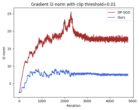
Figure 1: We conduct the preliminary experiment on Fashion-MNIST with CNN to illustrate the gradient $l_{2}$ norm during training.

G.2 Empirical Impact on Projection Dimension $k$

In Theorem 2 and  Corollary 1, we analyze the projection reconstruction error of subspace skewing, where we note that the eigen gap $\Delta_{k}$ is related to the choice of projection dimension $k$, so we verify the impact of different $k$ on model performance in Fig. 2. By setting $k$ to $\{10,25,50,75,100,150\}$, we observe that in the FMNIST dataset, the optimal $k$ value is around 100. For $k\in[25,100]$, the model accuracy is close, while larger or smaller $k$ could lead to significant performance degradation.

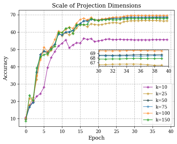
Figure 2: The experiment on Fashion-MNIST with CNN to illustrate the impact of different $k$ on model utility.

G.3 Empirical Impact on Projection Frequency

We are accustomed to selecting public data to generate projection matrix per round, which actually incurs additional computational overhead, even though some library functions (torch.svd in Pytorch) can currently alleviate this problem. Therefore, we attempt to generate projection at intervals over the iterations, that is, set the projection interval $\beta$ and use the same projection matrix from the $t$-th iteration to the $(t+\beta-1)$-th iteration. We test different projection intervals in the experiment and obtain the results as shown in Fig. 3.

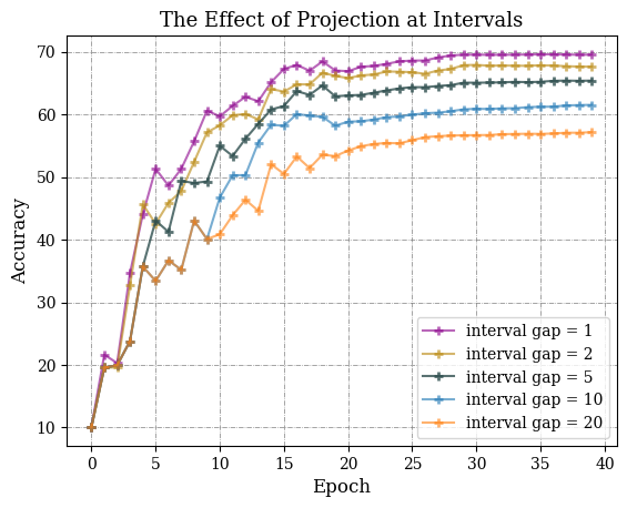
Figure 3: The experiment on Fashion-MNIST with CNN to illustrate the impact of different projection intervals on model performance.

It can be seen that expanding the projection interval damages the model performance. However, under stricter requirements on computing resources and time overhead, properly adjusting the projection interval could keep the model utility acceptable.

G.4 Visualization for Gradient Distribution with Projection

We discussed the visualization of gradient distributions in Section 4.5 of the main text, and we attach more relevant experiments (Fig. 4 and Fig. 5) here to strengthen the reliability of our method.

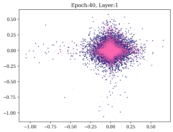
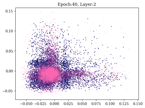
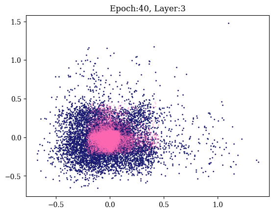
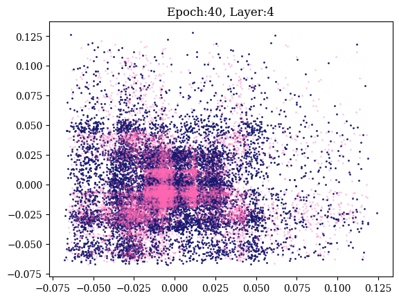
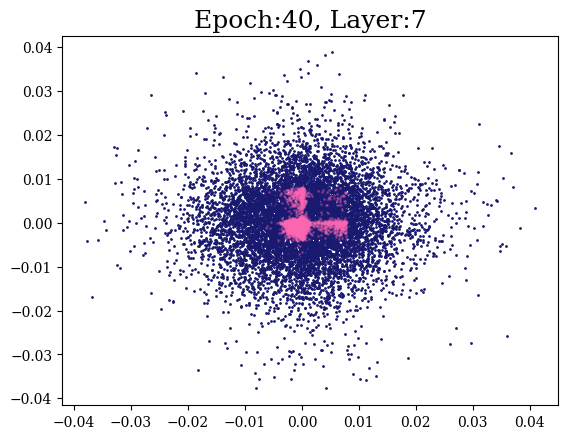
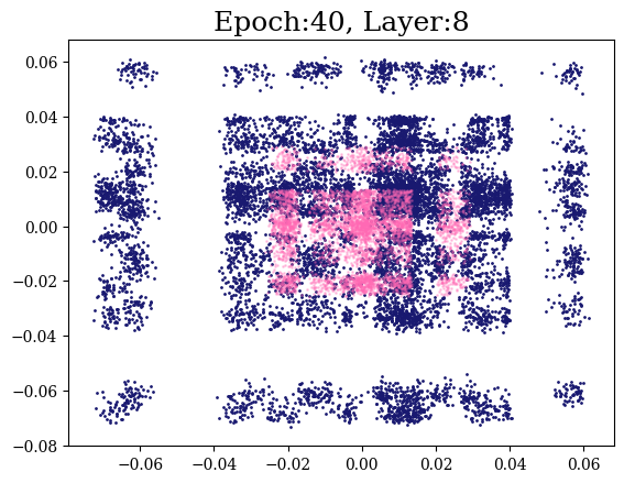
Figure 4: Gradient distributions with/without projection under the setting of $c=0.01$ and $\gamma$ = 1. The experiment is conducted on the CIFAR10 dataset with LeNet network.

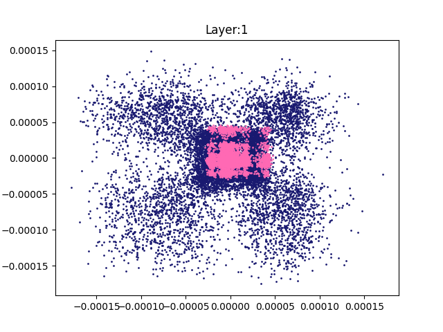
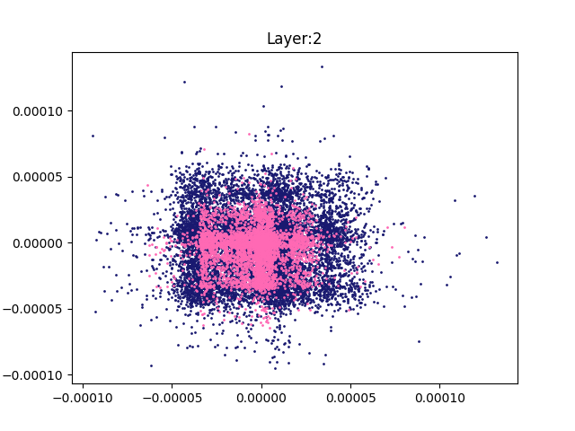
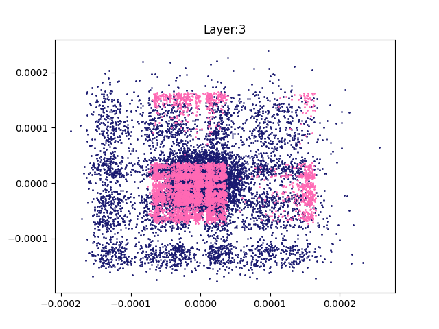
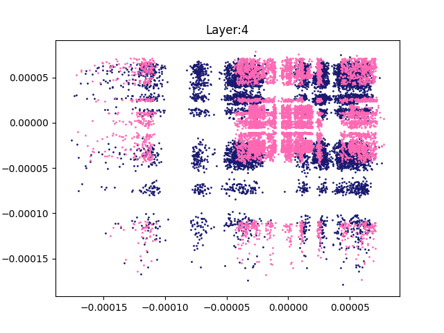
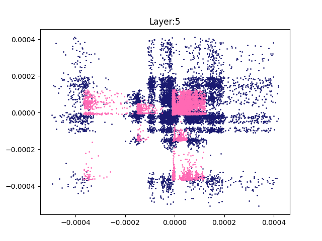
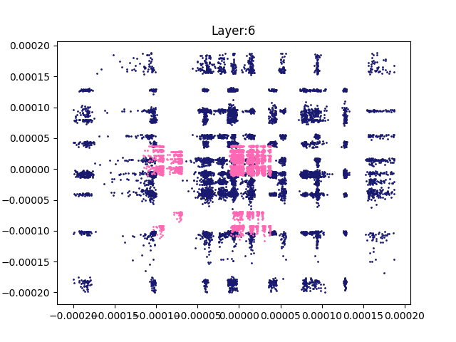
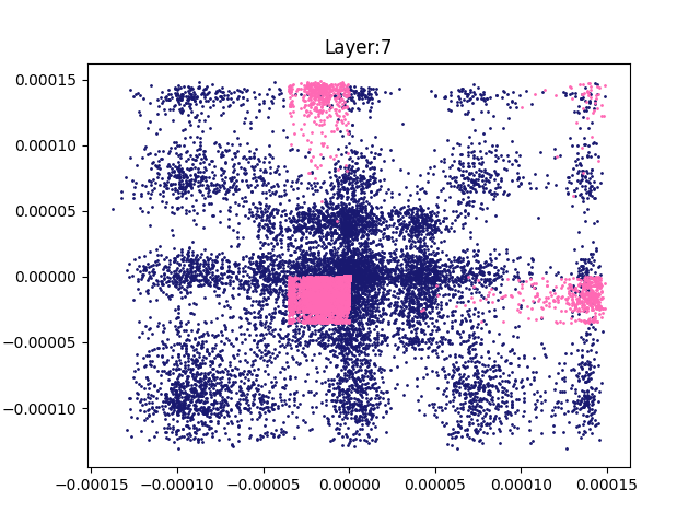
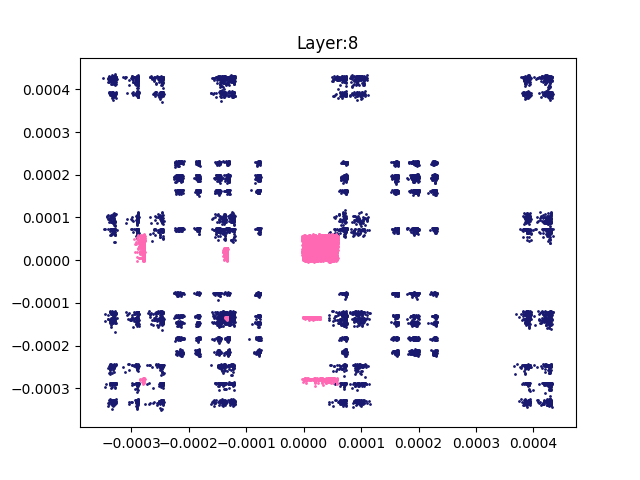
Figure 5: Gradient distributions with/without projection under the setting of $c=0.01$ and $\gamma$ = 1. The experiment is conducted on the MNIST dataset with CNN network.

G.5 Full Results of PCDP-SGD on Multiple Datasets

For MNIST and FMNIST, we fix $\delta=1e^{-5}$, set epsilon $\epsilon$ to $\{1.18,0.69,0.49,0.38,0.31,0.26,0.23\}$ for noise multiplier $\sigma\in\{6,10,14,18,22,26,30\}$. For CIFAR10, the epsilon $\epsilon$ is $\{4,1.8,1.18,0.69,0.49,0.38\}$ for noise multiplier $\sigma\in\{2,4,6,10,14,18\}$. Both MNIST and FMNIST are based on CNN network, and CIFAR10 is based on LeNet network. Here, we list out the complete results in Tabs. 2, 3 and 4. In RPDP-SGD, we set random projection dimension to 800 for MNIST and 1000 for FMNIST/CIFAR10. Additionally, we set the sparsity rate to 0.3 in RSDP-SGD.

Table 2: Test accuracy on MNIST of PCDP-SGD in the centralized scenario over 4 runs.

Dateset	MNIST-Accuracy %
Method	Privacy budget / Noise multiplier
	1.18 / 6	0.69 / 10	0.49 / 14	0.38 / 18	0.31 / 22	0.26 / 26	0.23 / 30
DP-SGD	91.91$\pm$0.56	87.85$\pm$1.61	79.39$\pm$2.09	66.09$\pm$1.62	50.51$\pm$3.16	42.10$\pm$3.27	34.43$\pm$2.62
PDP-SGD	88.73$\pm$0.47	88.24$\pm$0.49	87.00$\pm$1.24	84.74$\pm$0.89	83.59$\pm$0.45	80.16$\pm$1.30	76.88$\pm$2.22
RPDP-SGD	87.28 0.48	87.40$\pm$0.78	85.25$\pm$0.85	82.71$\pm$0.68	78.06$\pm$0.67	71.32$\pm$0.51	62.45$\pm$0.27
RSDP-SGD	91.17$\pm$0.59	86.79$\pm$0.96	76.86$\pm$0.71	62.39$\pm$1.73	49.44$\pm$1.43	39.82$\pm$0.67	30.92$\pm$1.68
PCDP-SGD	89.30$\pm$0.41	88.51$\pm$0.57	87.99$\pm$0.83	86.10$\pm$0.93	85.20$\pm$0.49	82.89$\pm$0.54	79.46$\pm$1.16

Table 3: Test accuracy on FMNIST of PCDP-SGD in the centralized scenario over 4 runs.

Dateset	FMNIST-Accuracy %
Method	Privacy budget / Noise multiplier
	1.18 / 6	0.69 / 10	0.49 / 14	0.38 / 18	0.31 / 22	0.26 / 26	0.23 / 30
DP-SGD	74.49$\pm$0.65	73.13$\pm$0.30	70.43$\pm$0.23	67.21$\pm$0.39	63.24$\pm$0.33	55.82$\pm$1.94	48.74$\pm$3.19
PDP-SGD	71.96$\pm$0.62	71.56$\pm$0.68	70.87$\pm$0.35	70.47$\pm$0.28	69.54$\pm$0.61	68.21$\pm$0.93	66.21$\pm$1.70
RPDP-SGD	70.57 0.37	70.81$\pm$0.14	70.43$\pm$0.34	69.58$\pm$0.13	67.83$\pm$0.69	65.59$\pm$1.38	63.86$\pm$0.32
RSDP-SGD	72.96$\pm$0.28	72.32$\pm$0.36	69.87$\pm$0.49	64.74$\pm$0.28	60.40$\pm$0.95	52.78$\pm$2.85	45.52$\pm$3.63
PCDP-SGD	72.21$\pm$0.63	71.83$\pm$0.62	71.28$\pm$0.41	70.48$\pm$0.35	70.06$\pm$0.53	69.65$\pm$1.12	68.18$\pm$0.94

Table 4: Test accuracy on CIFAR10 of PCDP-SGD in the centralized scenario over 4 runs.

Dateset	CIFAR10-Accuracy %
Method	Privacy budget / Noise multiplier
	4.00 / 2	1.80 / 4	1.18 / 6	0.69 / 10	0.49 / 14	0.38 / 18
DP-SGD	45.56	39.37	32.41	24.60	19.57	16.33
PDP-SGD	34.75	34.24	33.91	32.09	31.35	28.68
RPDP-SGD	34.75	45.44	31.02	25.80	25.55	25.01
RSDP-SGD	44.11	38.81	29.87	17.25	13.89	12.86
PCDP-SGD	35.66	35.30	34.84	33.23	30.48	28.85

G.6 Clipping Threshold and Learning Rate

As shown in Fig. 6, we conduct experiments under different parameters and find that PCDP-SGD performs stable and excellent at small clipping thresholds. By setting $c$ to $\{5,1,0.5,0.1,0.05,0.01,0.005,0.001,0.0001\}$ and $\gamma$ to $\{100,10,5,1,0.5,0.1,0.05,0.01\}$, we obtain that when the clipping threshold is small enough, the model utility presents a diagonal phenomenon mentioned in section 4.2 in which the clipping threshold and the learning rate are coupled.

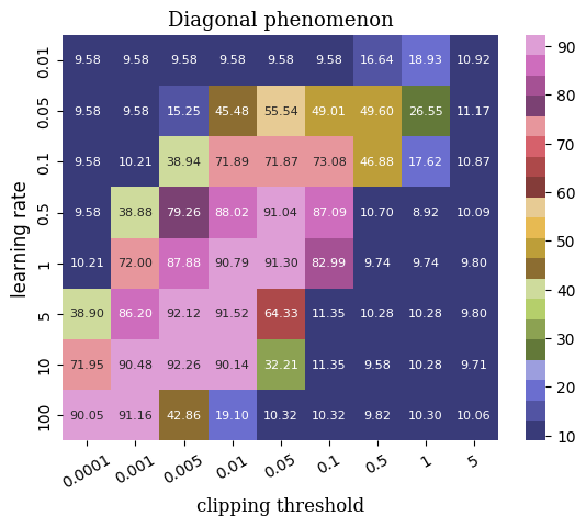
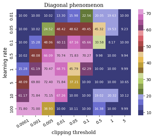
Figure 6: Diagonal phenomenon of clipping threshold and learning rate for MNIST (left) and FMNIST (right).

G.7 Independent and Dependent Segmentation

There are two ways to partition the auxiliary dataset: 1) Divide the auxiliary dataset into $T$ independent batch size blocks (IBS). 2) Each round extracts random batch size data block (RBS) from auxiliary data to generate projection. From Fig. 7, experimental results show that the size of auxiliary datasets (Aux=$m$) is positively correlated with model performance due to the reduction of projection reconstruction errors with the factor of $\mathcal{O}(\frac{1}{\sqrt{m}})$. Moreover, the results of the independent split are better than the dependent method under the same batch size, but the independent method requires larger auxiliary dataset.

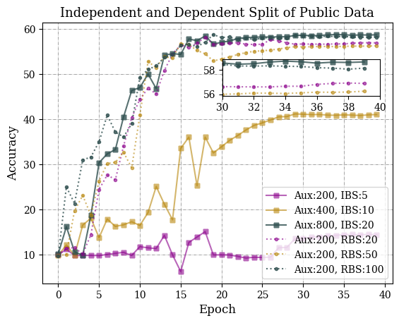
Figure 7: Comparison of independent and dependent segmentation for FMNIST.

G.8 Communication Efficiency of FedPCDP

We characterized the FedPCDP communication mechanism using the decomposition projection matrix in Algorithm 2. Specifically, FedPCDP first calculates the offset of the local client over $K$ iterations, i.e., $x-y^{i}_{K}$. We know that projection is essentially the product of two eigenspace matrices. Due to the public nature of projection, we reserve the common eigenspace on the clients and server, i.e., $V^{r}_{K}$, the clients utilize the transposition of $V^{r}_{K}$ for gradient information dimensionality reduction. Considering that local training is also limited to low-dimensional eigenspace, the method of transmission through projection will not cause excessive loss of gradient information. On the contrary, if the local training does not use projection, but only performs projection in the communication round, it will cause a “hard landing” of gradient, as shown in the simplified version of PFA. Next, the server uses $V^{r}_{K}$ to restore the received gradient and adds it to the historical global parameters to obtain the new global parameters.
We analyze the proportion of actual reduction in communication costs: assuming the model has $N$ layers in total, the flattening dimension of the $i$-th layer network channel is $p_{i}$, and the projection dimension is $k$, when $k>p_{i}$ (such as output layer), $k=p_{i}$. So, it can be concluded that the single client communication cost per round is $\sum^{N}_{i}p_{i}$ Bytes, but the cost under FedPCDP is less than $Nk$ Bytes. Taking Fashion-MNIST CNN (two-layer convolution + two-layer MLP) as an example, assuming a default projection of 100, the original client’s communication overhead is 25KB per round, while that of FedPCDP is 0.48 KB. Considering the increase in clients and communication rounds, the overall communication overhead can be significantly saved, thereby optimizing communication efficiency.

References

• Abadi et al. [2016] Martin Abadi, Andy Chu, Ian Goodfellow, H Brendan McMahan, Ilya Mironov, Kunal Talwar, and Li Zhang. Deep learning with differential privacy. In Proceedings of the 2016 ACM SIGSAC conference on computer and communications security, pages 308–318, 2016.
• Adnan et al. [2022] Mohammed Adnan, Shivam Kalra, Jesse C Cresswell, Graham W Taylor, and Hamid R Tizhoosh. Federated learning and differential privacy for medical image analysis. Scientific reports, 12(1):1953, 2022.
• Alon et al. [2019] Noga Alon, Raef Bassily, and Shay Moran. Limits of private learning with access to public data. Advances in neural information processing systems, 32, 2019.
• Andrew et al. [2021] Galen Andrew, Om Thakkar, Brendan McMahan, and Swaroop Ramaswamy. Differentially private learning with adaptive clipping. Advances in Neural Information Processing Systems, 34:17455–17466, 2021.
• Bassily et al. [2020] Raef Bassily, Albert Cheu, Shay Moran, Aleksandar Nikolov, Jonathan Ullman, and Steven Wu. Private query release assisted by public data. In International Conference on Machine Learning, pages 695–703. PMLR, 2020.
• Blocki et al. [2012] Jeremiah Blocki, Avrim Blum, Anupam Datta, and Or Sheffet. The johnson-lindenstrauss transform itself preserves differential privacy. In 2012 IEEE 53rd Annual Symposium on Foundations of Computer Science, pages 410–419. IEEE, 2012.
• Bloom et al. [2017] Cara Bloom, Joshua Tan, Javed Ramjohn, and Lujo Bauer. Self-driving cars and data collection: Privacy perceptions of networked autonomous vehicles. In Thirteenth Symposium on Usable Privacy and Security (SOUPS 2017), pages 357–375, 2017.
• Bu et al. [2020] Zhiqi Bu, Jinshuo Dong, Qi Long, and Weijie J Su. Deep learning with gaussian differential privacy. Harvard data science review, 2020(23):10–1162, 2020.
• Bu et al. [2022] Zhiqi Bu, Yu-Xiang Wang, Sheng Zha, and George Karypis. Automatic clipping: Differentially private deep learning made easier and stronger. arXiv preprint arXiv:2206.07136, 2022.
• Carlini et al. [2023] Nicholas Carlini, Jamie Hayes, Milad Nasr, Matthew Jagielski, Vikash Sehwag, Florian Tramer, Borja Balle, Daphne Ippolito, and Eric Wallace. Extracting training data from diffusion models. arXiv preprint arXiv:2301.13188, 2023.
• Chen et al. [2020] Xiangyi Chen, Steven Z Wu, and Mingyi Hong. Understanding gradient clipping in private sgd: A geometric perspective. Advances in Neural Information Processing Systems, 33:13773–13782, 2020.
• Cheng et al. [2022] Anda Cheng, Peisong Wang, Xi Sheryl Zhang, and Jian Cheng. Differentially private federated learning with local regularization and sparsification. In Proceedings of the IEEE/CVF Conference on Computer Vision and Pattern Recognition, pages 10122–10131, 2022.
• Dangel et al. [2020] Felix Dangel, Frederik Kunstner, and Philipp Hennig. BackPACK: Packing more into backprop. In International Conference on Learning Representations, 2020.
• Doshi and Yilmaz [2022] Keval Doshi and Yasin Yilmaz. Federated learning-based driver activity recognition for edge devices. In Proceedings of the IEEE/CVF Conference on Computer Vision and Pattern Recognition, pages 3338–3346, 2022.
• Dwork et al. [2006] Cynthia Dwork, Frank McSherry, Kobbi Nissim, and Adam Smith. Calibrating noise to sensitivity in private data analysis. In Theory of Cryptography: Third Theory of Cryptography Conference, TCC 2006, New York, NY, USA, March 4-7, 2006. Proceedings 3, pages 265–284. Springer, 2006.
• Golatkar et al. [2022] Aditya Golatkar, Alessandro Achille, Yu-Xiang Wang, Aaron Roth, Michael Kearns, and Stefano Soatto. Mixed differential privacy in computer vision. In Proceedings of the IEEE/CVF Conference on Computer Vision and Pattern Recognition, pages 8376–8386, 2022.
• Gur-Ari et al. [2018] Guy Gur-Ari, Daniel A Roberts, and Ethan Dyer. Gradient descent happens in a tiny subspace. arXiv preprint arXiv:1812.04754, 2018.
• Hu et al. [2020] Rui Hu, Yanmin Gong, and Yuanxiong Guo. Federated learning with sparsification-amplified privacy and adaptive optimization. arXiv preprint arXiv:2008.01558, 2020.
• Hu et al. [2019] Wenqing Hu, Chris Junchi Li, Lei Li, and Jian-Guo Liu. On the diffusion approximation of nonconvex stochastic gradient descent. Annals of Mathematical Sciences and Applications, 4(1), 2019.
• Ji et al. [2022] Jiazhen Ji, Huan Wang, Yuge Huang, Jiaxiang Wu, Xingkun Xu, Shouhong Ding, ShengChuan Zhang, Liujuan Cao, and Rongrong Ji. Privacy-preserving face recognition with learnable privacy budgets in frequency domain. In European Conference on Computer Vision, pages 475–491. Springer, 2022.
• Karimireddy et al. [2020] Sai Praneeth Karimireddy, Satyen Kale, Mehryar Mohri, Sashank Reddi, Sebastian Stich, and Ananda Theertha Suresh. Scaffold: Stochastic controlled averaging for federated learning. In International conference on machine learning, pages 5132–5143. PMLR, 2020.
• Li et al. [2018] Chunyuan Li, Heerad Farkhoor, Rosanne Liu, and Jason Yosinski. Measuring the intrinsic dimension of objective landscapes. arXiv preprint arXiv:1804.08838, 2018.
• Li et al. [2021a] Qinbin Li, Bingsheng He, and Dawn Song. Model-contrastive federated learning. In Proceedings of the IEEE/CVF conference on computer vision and pattern recognition, pages 10713–10722, 2021a.
• Li et al. [2020a] Tian Li, Anit Kumar Sahu, Manzil Zaheer, Maziar Sanjabi, Ameet Talwalkar, and Virginia Smith. Federated optimization in heterogeneous networks. Proceedings of Machine learning and systems, 2:429–450, 2020a.
• Li et al. [2020b] Xinyan Li, Qilong Gu, Yingxue Zhou, Tiancong Chen, and Arindam Banerjee. Hessian based analysis of sgd for deep nets: Dynamics and generalization. In Proceedings of the 2020 SIAM International Conference on Data Mining, pages 190–198. SIAM, 2020b.
• Li et al. [2021b] Xuechen Li, Florian Tramer, Percy Liang, and Tatsunori Hashimoto. Large language models can be strong differentially private learners. arXiv preprint arXiv:2110.05679, 2021b.
• Liu et al. [2021] Junxu Liu, Jian Lou, Li Xiong, Jinfei Liu, and Xiaofeng Meng. Projected federated averaging with heterogeneous differential privacy. Proceedings of the VLDB Endowment, 15(4):828–840, 2021.
• Mandt et al. [2016] Stephan Mandt, Matthew Hoffman, and David Blei. A variational analysis of stochastic gradient algorithms. In International conference on machine learning, pages 354–363. PMLR, 2016.
• McMahan et al. [2017] Brendan McMahan, Eider Moore, Daniel Ramage, Seth Hampson, and Blaise Aguera y Arcas. Communication-efficient learning of deep networks from decentralized data. In Artificial intelligence and statistics, pages 1273–1282. PMLR, 2017.
• Mcsherry [2004] Frank Mcsherry. Spectral methods for data analysis. PhD thesis, University of Washington., 2004.
• Mehta et al. [2022] Harsh Mehta, Abhradeep Thakurta, Alexey Kurakin, and Ashok Cutkosky. Large scale transfer learning for differentially private image classification. arXiv preprint arXiv:2205.02973, 2022.
• Meng et al. [2021] Qiang Meng, Feng Zhou, Hainan Ren, Tianshu Feng, Guochao Liu, and Yuanqing Lin. Improving federated learning face recognition via privacy-agnostic clusters. In International Conference on Learning Representations, 2021.
• Pichapati et al. [2019] Venkatadheeraj Pichapati, Ananda Theertha Suresh, Felix X Yu, Sashank J Reddi, and Sanjiv Kumar. Adaclip: Adaptive clipping for private sgd. arXiv preprint arXiv:1908.07643, 2019.
• Sagun et al. [2017] Levent Sagun, Utku Evci, V Ugur Guney, Yann Dauphin, and Leon Bottou. Empirical analysis of the hessian of over-parametrized neural networks. arXiv preprint arXiv:1706.04454, 2017.
• Shi et al. [2023] Yifan Shi, Yingqi Liu, Kang Wei, Li Shen, Xueqian Wang, and Dacheng Tao. Make landscape flatter in differentially private federated learning. In Proceedings of the IEEE/CVF Conference on Computer Vision and Pattern Recognition, pages 24552–24562, 2023.
• Simsekli et al. [2019] Umut Simsekli, Levent Sagun, and Mert Gurbuzbalaban. A tail-index analysis of stochastic gradient noise in deep neural networks. In International Conference on Machine Learning, pages 5827–5837. PMLR, 2019.
• Sun et al. [2023] Jiankai Sun, Xin Yang, Yuanshun Yao, Junyuan Xie, Di Wu, and Chong Wang. Dpauc: Differentially private auc computation in federated learning. In Proceedings of the AAAI Conference on Artificial Intelligence, pages 15170–15178, 2023.
• Talagrand [2014] Michel Talagrand. Upper and lower bounds for stochastic processes. Springer, 2014.
• Xia et al. [2023] Tianyu Xia, Shuheng Shen, Su Yao, Xinyi Fu, Ke Xu, Xiaolong Xu, and Xing Fu. Differentially private learning with per-sample adaptive clipping. In Proceedings of the AAAI Conference on Artificial Intelligence, pages 10444–10452, 2023.
• Yang et al. [2022] Xiaodong Yang, Huishuai Zhang, Wei Chen, and Tie-Yan Liu. Normalized/clipped sgd with perturbation for differentially private non-convex optimization. arXiv preprint arXiv:2206.13033, 2022.
• Zhang et al. [2019] Jingzhao Zhang, Tianxing He, Suvrit Sra, and Ali Jadbabaie. Why gradient clipping accelerates training: A theoretical justification for adaptivity. arXiv preprint arXiv:1905.11881, 2019.
• Zhang et al. [2022] Xinwei Zhang, Xiangyi Chen, Mingyi Hong, Zhiwei Steven Wu, and Jinfeng Yi. Understanding clipping for federated learning: Convergence and client-level differential privacy. In International Conference on Machine Learning, ICML 2022, 2022.
• Zhou et al. [2021] Yingxue Zhou, Steven Wu, and Arindam Banerjee. Bypassing the ambient dimension: Private sgd with gradient subspace identification. In International Conference on Learning Representations, 2021.
• Zhu and Blaschko [2021] Junyi Zhu and Matthew B Blaschko. Improving differentially private sgd via randomly sparsified gradients. arXiv e-prints, pages arXiv–2112, 2021.
• Zhu et al. [2019] Zhanxing Zhu, Jingfeng Wu, Bing Yu, Lei Wu, and Jinwen Ma. The anisotropic noise in stochastic gradient descent: Its behavior of escaping from sharp minima and regularization effects. In International Conference on Machine Learning, pages 7654–7663. PMLR, 2019.
• Ziller et al. [2021] Alexander Ziller, Dmitrii Usynin, Rickmer Braren, Marcus Makowski, Daniel Rueckert, and Georgios Kaissis. Medical imaging deep learning with differential privacy. Scientific Reports, 11(1):13524, 2021.
\thetitle