Memory-Efficient Optical Flow via Radius-Distribution Orthogonal Cost Volume

Abstract

The full 4D cost volume in Recurrent All-Pairs Field Transforms (RAFT) or global matching by Transformer achieves impressive performance for optical flow estimation. However, their memory consumption increases quadratically with input resolution, rendering them impractical for high-resolution images. In this paper, we present MeFlow, a novel memory-efficient method for high-resolution optical flow estimation. The key of MeFlow is a recurrent local orthogonal cost volume representation, which decomposes the 2D search space dynamically into two 1D orthogonal spaces, enabling our method to scale effectively to very high-resolution inputs. To preserve essential information in the orthogonal space, we utilize self attention to propagate feature information from the 2D space to the orthogonal space. We further propose a radius-distribution multi-scale lookup strategy to model the correspondences of large displacements at a negligible cost. We verify the efficiency and effectiveness of our method on the challenging Sintel and KITTI benchmarks, and real-world 4K ($2160\!\times\!3840$) images. Our method achieves competitive performance on both Sintel and KITTI benchmarks, while maintaining the highest memory efficiency on high-resolution inputs. Code is available at https://github.com/gangweiX/MeFlow.

1 Introduction

Optical flow, which estimates per-pixel 2D motion between successive two images, is a fundamental task for many applications such as action recognition [24, 28], video processing [42, 44] and autonomous driving [22]. Despite decades of research, accurately estimating optical flow with high memory and computational efficiency, in particular for high-resolution images (more than 4K resolution), remains very challenging.

State-of-the-art optical flow estimate methods [6, 29, 34] mainly leverage deep learning frameworks with an essential component called cost volume. The pioneering deep learning-based optical flow method FlowNetC [6], employs convolutional neural networks (CNNs) to extract feature maps. It constructs a cost volume by computing correlations between each pixel in the source image and its potential correspondences within a 2D search window of the target image. After that, relative pixel displacements are inferred and regressed from the cost volume via CNNs. Motivated by the success of FlowNetC, a serial of methods [13, 29, 10, 34] have been proposed and achieved the state-of-the-art performance.

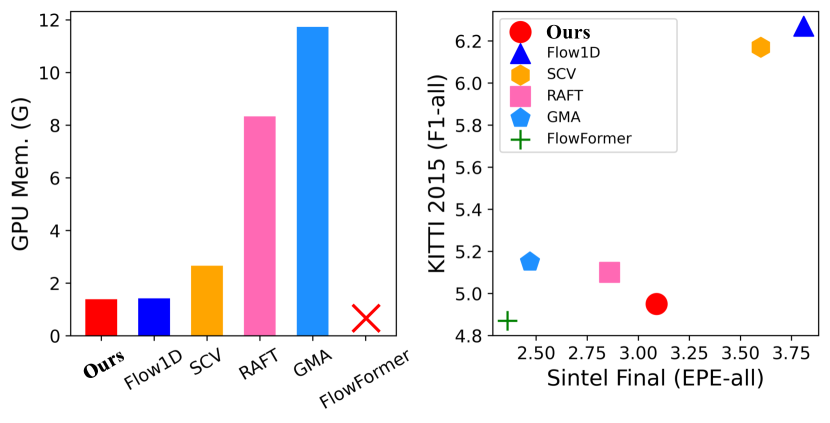
Figure 1: Comparison with state-of-the-art optical flow methods. Left: GPU memory consumption on 1080p ($1080\!\times\!1920$) resolution inputs. Right: Results on Sintel and KITTI benchmarks. Our MeFlow achieves the highest memory efficiency and competitive accuracy. The red cross $\times$ denotes that FlowFormer [9] causes an out-of-memory error on our 24G GPU.

A recent and notable work is RAFT [34] which computes all-pairs correlations to form a full 4D cost volume. As the full 4D cost volume can encode complete pairwise matching information, RAFT achieves impressive performance on several established benchmarks. However, the complexity of the 4D cost volume, i.e., $\mathcal{O}(H\!\times\!W\!\times\!H\!\times\!W)$, grows quadratically with input image resolution, preventing its application to very high-resolution images. To reduce the memory cost, SCV [15] proposes a sparse cost volume that only stores the top-k correlations for each pixel. However, this approach may miss true matches for textureless and ambiguous regions, and in turn yield a 21.0% performance degradation on KITTI compared to RAFT. Subsequently, Flow1D [39] constructs two 3D cost volumes to replace RAFT’s 4D cost volume. To construct two 3D cost volumes, Flow1D decomposes a 2D search space into two orthogonal 1D search spaces by attention, as shown in Fig. 2. However, global attention in Flow1D is position-sensitive, yielding miss detection of true matches with large motions. As a result, Flow1D struggles to handle large motions, shown in Fig. 3 and Tab. 6.

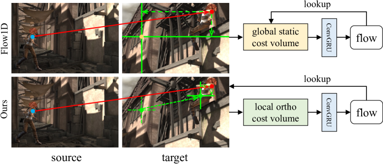
Figure 2: Comparison of our local orthogonal cost volume and the global static cost volume in Flow1D [39]. Flow1D only searches two static orthogonal lines (green lines) for every pixel in source image. In contrast, our method can dynamically search the entire 2D space based on the current updated flow (green point).

In this paper, we introduce a novel memory-efficient network for high-resolution optical flow estimation, named MeFlow. The core of MeFlow is a novel Local Orthogonal Cost Volume (LOV) that decomposes the 2D search space dynamically into two 1D orthogonal spaces. Unlike Flow1D which constructs global static cost volume, our LOV is a local dynamic cost volume that is built recurrently based on the current updated flow (shown in Fig. 2).

Our LOV is constructed via the following three steps (Fig. 4). First, we apply 1D local attention to the target feature to generate the vertically attended feature and horizontally attended feature. Since a pixel is more likely to belong to the same category as its neighboring pixels than those far away, this local attention can propagate reliable and effective information to the surroundings. Second, in each iteration, we index vertically attended feature and horizontally attended feature along the orthogonal direction based on the current flow estimation. Finally, we perform 1D correlation between these flow-indexed attended target feature and the source image feature to construct LOV, which can model 2D space correspondences.

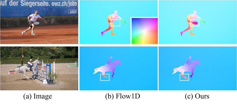
Figure 3: Comparisons with Flow1D [39] on DAVIS dataset. Flow1D struggles to handle large motions. In contrast, our method performs well in these regions. Flow visualization is based on the color wheel shown on the corner of the first flow map.

Different from RAFT’s multi-scale 4D cost volume and Flow1D’s two 3D cost volumes that only need to be constructed once before GRU iteration, our local orthogonal cost volume needs to be built for each GRU iteration. Therefore, properly setting the value of search radius $R$ is crucial for achieving both accuracy and efficiency. Increasing $R$ can model large motions, but it also increases the computational cost. To address this issue, we propose a novel radius-distribution multi-scale (RDMS) orthogonal lookup strategy (Fig. 5). We index finer-resolution (e.g., 1/8) attended target features within a smaller search range and coarser-resolution (e.g., 1/16 and 1/32) features in the outer search region. The proposed RDMS strategy can handle large motions with less computational cost compared to RAFT’s multi-scale 4D cost volume (Fig. 5).

The complexity of our LOV is $\mathcal{O}(H\!\times\!W\!\times\!(4R\!+\!2))$, where $R$ (default value is 8) denotes radius-distribution lookup radius. In comparison, the complexity of the cost volume in RAFT and Flow1D is $\mathcal{O}(H\!\times\!W\!\times\!H\!\times\!W)$ and $\mathcal{O}(H\!\times\!W\!\times\!(H\!+\!W))$ respectively. For high-resolution inputs, $4R\!+\!2\ll H\!+\!W\ll H\!\times\!W$ indicates that our LOV has a smaller peak memory usage in inference compared to Flow1D and RAFT.

We demonstrate the efficiency and effectiveness of our approach on the challenging datasets including Sintel [2], KITTI [22], as well as the high-resolution DAVIS datasets [23, 3]. Our approach consumes $6\times$ less memory than RAFT on 1080p resolution images and can handle real-world 4K images with only 5.4G memory usage. RAFT can not handle 4K images due to causing an out-of-memory error on our 24G GPU. Meanwhile, we achieved better results than RAFT on the KITTI benchmark. Our method also outperforms almost all memory-efficient methods, e.g., exceeding Flow1D by 21.1% and SCV by 19.8% on the KITTI benchmark.

Our major contributions can be summarized as follows:

• We propose a novel local orthogonal cost volume, which dynamically encodes the correspondences in 2D space into two 1D orthogonal spaces, enabling our method to scale well to very high-resolution inputs.

• We propose a new radius-distribution multi-scale lookup strategy to efficiently model the correspondences of large displacements.

• We design a memory-efficient flow network, named MeFlow, which achieves the highest memory efficiency among all published methods and outperforms almost all memory-efficient methods on the challenging Sintel and KITTI benchmarks.

2 Related Work

Deep Flow Methods

Deep convolutional neural networks have shown great success in optical flow estimate tasks. FlowNet [6] is an pioneer end-to-end CNN-based network for optical flow, which inspires a serial of subsequent works [13, 29, 10]. FlowNet2 [13] introduces a warping operation and stacks multiple basic models to improve model capacity and performance. To further reduce model size and inference time, several methods [30, 11, 12] propose the coarse-to-fine cost volume pyramid. However, these methods tend to miss fast-moving small objects in the coarse stage. To address this issue, RAFT [34] proposes to construct an all-pairs 4D cost volume, recurrently indexing the cost values and optimizing them in the convolution GRU block to update optical flow. RAFT achieves the state-of-the-art performance on optical flow benchmarks. Based on the RAFT architecture, some recurrent methods [14, 18, 48, 27, 19, 20, 26, 25] have been proposed to further improve the accuracy. For example, GMA [14] and KPAFlow [18] aggregate global or local motion features via attention mechanism to resolve ambiguities caused by occlusions, yielding the state-of-the-art performance. However, due to the use of the 4D cost volume ($H\!\times\!W\!\times\!H\!\times\!W$), the memory consumption of these two methods grows quadratically with the input resolution, which makes them very difficult to scale to high-resolution images.

Memory-Efficient Flow Methods

Several recent works have designed efficient cost volume representations to replace the original 4D cost volume in RAFT [34] for processing high-resolution images. For example, SCV [15] constructs a sparse cost volume by computing the top-k correlations for each pixel. Flow1D [39] constructs two 3D cost volumes in the vertical and horizontal directions respectively to represent 4D spatial correlation. Even though they improve memory efficiency, they suffer from nontrivial loss of accuracy compared to the original 4D cost volume in RAFT. DIP [49] introduces the idea of the conventional method Patchmatch into the end-to-end optical flow network. Benefiting from propagation and local search of Patchmatch which can effectively avoid the 4D cost volume construction, DIP can achieve high-precision results with a low memory cost. However, sequential ConvGRU modules (i.e., alternating the propagation block and the local search block) in DIP are time-consuming, yielding a $2.4\times$ slower speed than our method for 1080p ($1080\times 1920$) resolution images. Among these memory-efficient methods [15, 39, 49], our method achieves the highest efficiency in memory while achieving the state-of-the-art performance on the KITTI benchmark.

Attention mechanism

Attention has achieved great success in many vision tasks [16, 7, 8, 35, 4, 32, 14, 37, 40, 38] due to its ability to model long-range dependencies. For example, CCNet [8] proposes efficient criss-cross attention to aggregate contextual information. GMA [14] uses attention to aggregate global motion features, and GMFlow [40] exploits the cross attention to obtain discriminative features for matching. Flow1D [39] uses 1D cross attention for global feature propagation and then computes 1D correlation. However, such global propagation in Flow1D is position sensitive, yielding miss detection of true matches with large displacements. Instead, the local attention in our MeFlow can propagate more reliable and effective information.

3 MeFlow

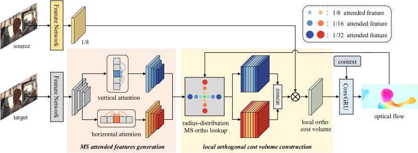
Figure 4: Overview of the proposed MeFlow. We apply vertical and horizontal attention to the multi-scale target features to generate multi-scale attended features. Then, in each iteration, we index the multi-scale vertically attended features and horizontally attended features along the horizontal and vertical direction respectively based on the current updated flow (green point). Specially, the proposed radius-distribution multi-scale (MS) orthogonal lookup can index finer-resolution features at small radius and coarser-resolution at large radius. Finally, we construct a dynamic orthogonal cost volume by performing 1D correlation between the source image feature and the dynamically indexed attended features.

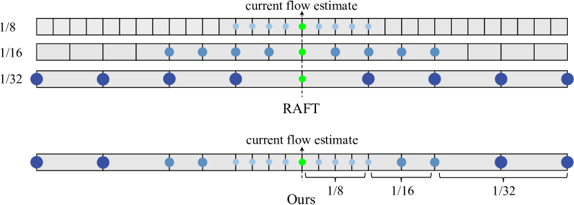
Figure 5: RAFT’s multi-scale strategy v.s. our radius-distribution multi-scale strategy.

Optical flow is essentially a 2D search problem, which has the quadratic complexity with respect to the 2D search window. Thus, directly searching in the 2D space could become computationally intractable for large displacements, limiting its application to high-resolution images which are ubiquitous in practical scenarios due to the popularity of high-definition cameras.

This section presents MeFlow, which can handle high-resolution images with a low memory cost by decomposing the 2D search space dynamically into two 1D orthogonal spaces. Our MeFlow mainly consists of two components: 1) Multi-scale Attended Features Generation and 2) Local Orthogonal Cost Volume Construction. Next, we will introduce the details of each component.

3.1 Multi-Scale Attended Features Generation

Given source and target images ${\textbf{I}}_{s}$ and ${\textbf{I}}_{t}$, we first extract $8\times$ downsampled features ${\textbf{F}}_{s},{\textbf{F}}_{t}\in\mathbb{R}^{H\times W\times D}$ with a weight-sharing feature network, where $H,W$ and $D$ denote height, width and feature dimension, respectively. Following RAFT [34], the feature network consists of 6 residual blocks, 2 at 1/2 resolution, 2 at 1/4 resolution, and 2 at 1/8 resolution.

To produce multi-scale attended target features, we apply one and two average pooling operations with a $2\times 2$ kernel size to the target feature ${\textbf{F}}_{t}$ to obtain 1/16 resolution target feature ${\textbf{F}}_{t}^{d1}$ and 1/32 resolution target feature ${\textbf{F}}_{t}^{d2}$ respectively. Then, we use vertical and horizontal attention (Fig. 4) on the these generated target features (i.e. ${\textbf{F}}_{t}$, ${\textbf{F}}_{t}^{d1}$, ${\textbf{F}}_{t}^{d2}$) to obtain vertically attended target features $\hat{\textbf{F}}_{t,v}$, $\hat{\textbf{F}}_{t,v}^{d1}$, $\hat{\textbf{F}}_{t,v}^{d2}$ and horizontally attended target features $\hat{\textbf{F}}_{t,h}$ $\hat{\textbf{F}}_{t,h}^{d1}$, $\hat{\textbf{F}}_{t,h}^{d2}$. In vertically attended target features, every feature at a point P contains feature information of a set of points which lie on the same column of P. Similarly, in horizontally attended target features, every feature at a point P contains feature information of a set of points which lie on the same row of P. Here, we detail the generation process of $\hat{\textbf{F}}_{t,v}$, and the generation process of other attended target features is similar.

Given the target feature ${\textbf{F}}_{t}$, we first apply two convolutional layers with $1\!\times\!1$ filters to ${\textbf{F}}_{t}$ to generate two feature maps Q and K, respectively, where Q, ${\textbf{K}}\in\mathbb{R}^{H\times W\times D}$. Then we unfold K with radius $R_{0}$ along the vertical direction, and the unfolded K is denoted as ${\textbf{K}}_{u}\in\mathbb{R}^{(2R_{0}+1)\times H\times W\times D}$. We generate correlation matrix ${\textbf{M}}\in\mathbb{R}^{(2R_{0}+1)\times H\times W}$ by affinity operation,

$$\begin{split}{\textbf{M}}(h,w)&=\frac{{\textbf{Q}}(h,w){{\textbf{K}}_{u}^{T}}(h,w)}{\sqrt{D}}\in\mathbb{R}^{2R_{0}+1},\\ \end{split}$$ (1)

where $\frac{1}{\sqrt{D}}$ is a normalization factor to avoid large values. Then, we normalize the first dimension of M with the softmax to obtain attention maps ${\textbf{A}}\in\mathbb{R}^{(2R_{0}+1)\times H\times W}$,

$$\begin{split}{\textbf{A}}&=softmax({\textbf{M}}).\end{split}$$ (2)

Finally, the attended target feature $\hat{\textbf{F}}_{t,v}$ is computed by vertically aggregating ${\textbf{F}}_{t}$,

$$\begin{split}\hat{\textbf{F}}_{t,v}(h,w)&=\sum_{r=-R_{0}}^{R_{0}}{\textbf{A}}(r,h,w){\textbf{F}}_{t}(h+r,w).\end{split}$$ (3)

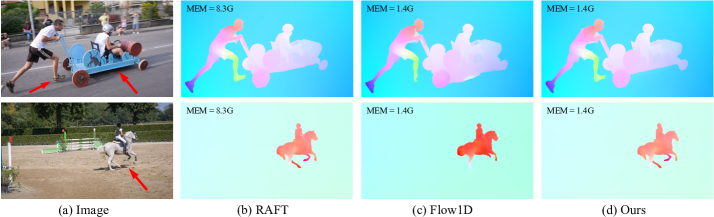
Figure 6: Comparisons on high-resolution ($1080\times 1920$) images from DAVIS. We achieve comparable results with RAFT [34] while consuming $6\times$ less memory. We achieve more accurate results than the SOTA memory-efficient Flow1D [39] (pointed by red arrows).

3.2 Local Orthogonal Cost Volume Construction

For each GRU iteration, we use the current optical flow to index a subset of multi-scale attended target features. Subsequently, we perform 1D correlation between these indexed target features and the source feature to construct a local orthogonal cost volume. Different from RAFT’s multi-scale 4D cost volume and Flow1D’s two 3D cost volumes that only need to be constructed once, our local orthogonal cost volume needs to be built for each GRU iteration. Thus, we propose a novel radius-distribution multi-scale strategy, which is more efficient than RAFT’s multi-scale strategy, shown in Fig. 5. Next, we will present the details of radius-distribution multi-scale strategy.

For a pixel at the position $(h,w)$ on the source image feature ${\textbf{F}}_{s}$, we find its corresponding position $(h^{\prime},w^{\prime})$ on the attended target image feature based on the current optical flow estimate ${\textbf{f}}=(f_{x},f_{y})$, i.e. $(h^{\prime},w^{\prime})=(h+f_{y},w+f_{x})$. Then, centered on the pixel position $(h^{\prime},w^{\prime})$, we index the multi-scale attended target features along the horizontal and vertical directions respectively. Specially, for the attended target features at 1/8, 1/16 and 1/32 resolution, the lookup radius is $R_{0}=4$, $R_{1}=2$ and $R_{3}=2$ respectively, and the total lookup radius is $R=R_{0}+R_{1}+R_{2}$ (Fig. 5). For example, with vertically attended target features $\hat{\textbf{F}}_{t,v}$, $\hat{\textbf{F}}_{t,v}^{d1}$ and $\hat{\textbf{F}}_{t,v}^{d2}$, we can calculate the horizontal cost volume ${\textbf{C}}_{h}$ along the horizontal direction,

$$\begin{split}{\textbf{C}}_{h}^{d0}(R\!+\!r_{0},h,w)&\!=\!\frac{1}{\sqrt{D}}{\textbf{F}}_{s}(h,w)\boldsymbol{\cdot}\hat{\textbf{F}}_{t,v}(h^{\prime},w^{\prime}\!+\!r_{0}),\\ {\textbf{C}}_{h}^{d1}(R\!+\!r_{1}\!/\!2,h,w)&\!=\!\frac{1}{\sqrt{D}}{\textbf{F}}_{s}(h,w)\boldsymbol{\cdot}\hat{\textbf{F}}_{t,v}^{d1}(h^{\prime}\!/\!2,w^{\prime}/2\!+\!r_{1}\!/\!2),\\ {\textbf{C}}_{h}^{d2}(R\!+\!r_{2}\!/\!4,h,w)&\!=\!\frac{1}{\sqrt{D}}{\textbf{F}}_{s}(h,w)\boldsymbol{\cdot}\hat{\textbf{F}}_{t,v}^{d2}(h^{\prime}\!/\!4,w^{\prime}/4\!+\!r_{2}\!/\!4),\\ {\textbf{C}}_{h}&=\text{Concat}\{{\textbf{C}}_{h}^{d0},{\textbf{C}}_{h}^{d1},{\textbf{C}}_{h}^{d2}\},\end{split}$$ (4)

where $\boldsymbol{\cdot}$ denotes the dot product, ${\textbf{C}}_{h}\in\mathbb{R}^{(2R+1)\times H\times W}$, and $r_{0}\!\in\!\{-4,-3,-2,-1,0,1,2,3,4\}$, $r_{1}\!\in\!\{-8,-6,6,8\}$, $r_{2}\!\in\!\{-16,-12,12,16\}$.

Model	Sintel (train)		KITTI (train)		Param (M)	$448\times 1024$		$1080\times 1920$
	Clean	Final	EPE	F1-all		Memory (G)	Time (ms)	Memory (G)	Time (ms)
Base ($(2r\!+\!1)^{2}$)	1.55	2.88	5.63	18.26	5.18	0.65	68	2.81	350
OC ($(2r\!+\!1)\!\times\!2$)	1.68	2.92	6.08	18.94	5.23	0.33	52	1.39	220
OC + OA	1.56	2.82	5.69	18.21	5.23	0.33	52	1.39	220
OC + OA + RDMS	1.49	2.75	5.31	16.65	5.23	0.33	65	1.39	260

Table 1: Ablation study. OC denotes orthogonal correlation, OA denotes orthogonal attention (i.e., vertical and horizontal attention), and RDMS denotes radius-distribution multi-scale lookup strategy. Base represents RAFT’s alternate implementation (lower memory cost). All models are trained on FlyingChairs and FlyingThings3D. The final model, OC+OA+RDMS, is denoted as MeFlow.

Similar to horizontal cost volume $\textbf{C}_{h}$, we perform vertical correlation on horizontally attended target features $\hat{\textbf{F}}_{t,h}$, $\hat{\textbf{F}}_{t,h}^{d1}$ and $\hat{\textbf{F}}_{t,h}^{d2}$ to obtain the vertical cost volume ${\textbf{C}}_{v}\in\mathbb{R}^{(2R+1)\times H\times W}$. Finally, we obtain the local orthogonal cost volume ${\textbf{C}}_{o}\in\mathbb{R}^{(4R+2)\times H\times W}$ by concatenating ${\textbf{C}}_{h}$ and ${\textbf{C}}_{v}$,

$$\begin{split}{\textbf{C}}_{o}&=\text{Concat}\{{\textbf{C}}_{h},{\textbf{C}}_{v}\}.\end{split}$$ (5)

The local orthogonal cost volume $\textbf{C}_{o}$ can model efficiently multi-scale 2D correspondences. Compared to RAFT’s alternate implementation, which needs to search 243 (i.e. $(2\times 4+1)^{2}\times 3$) target feature vectors for each position on the source image, our method only needs to search 34 (i.e. $4\times 8+2$) target feature vectors to model correspondences within the same scope, which is only 1/7 of RAFT (see Fig. 5).

3.3 Network Architecture

Fig. 4 presents the architecture of our MeFlow. Following RAFT [34], we extract $8\times$ downsampled features for source and target image by a feature network, and a context feature is also extracted from the source image with an additional context network. For brevity, we omit the context network. Next, we obtain target image features at three resolutions (i.e. 1/8, 1/16 and 1/32 resolution) through pooling operations, and perform vertical and horizontal attention on them respectively to generate multi-scale vertically attended features and horizontally attended features. In each iteration, we index multi-scale attended features along an orthogonal direction with the current flow estimation. Then we construct the local orthogonal cost volume by performing 1D correlation between the source image feature and the dynamically indexed attended target features. The local orthogonal cost volume, together with the current flow estimation and context feature, is then fed to a ConvGRU to update the current flow estimation.

Method	Sintel (train)		KITTI (train)		KITTI (test) F1-all	Param (M)	Memory (G)
	Clean	Final	EPE	F1-all			$448\times 1024$	$1080\times 1920$
RAFT [34]	1.43	2.71	5.04	17.40	5.10	5.26	0.48	8.33
FlowNet2 [13]	2.02	3.14	10.06	30.37	11.48	162.52	1.31	3.61
PWC-Net [29]	2.55	3.93	10.35	33.67	9.80	9.37	0.86	1.57
Flow1D [39]	1.98	3.27	6.69	22.95	6.27	5.73	0.34	1.42
MeFlow (Ours)	1.49	2.75	5.31	16.65	4.95	5.23	0.33	1.39

Table 2: Comparisons with existing representative methods. Memory and inference time are measured for $448\times 1024$ and $1080\times 1920$ resolutions on our RTX 3090 GPU, and the GRU-based iteration numbers are 12 for RAFT, Flow1D and our MeFlow. Bold: Best, Underscore: Second best.

3.4 Loss Function

Following RAFT [34], we supervised our network using the $l_{1}$ loss between the predicted and ground truth flow over the full sequence of predictions, {$\textbf{f}_{1}$,$\cdots$, $\mathbf{f}_{N}$}, with exponentially increasing weights. Given ground truth flow $\mathbf{f}_{gt}$, the loss is defined as,

$$\mathcal{L}=\sum_{i=1}^{N}\gamma^{N-i}||\mathbf{f}_{i}-\mathbf{f}_{gt}||_{1},$$ (6)

where we set $\gamma=0.8$ in our experiments.

4 Experiments

4.1 Experimental Setup

Datasets and evaluation setup. We evaluate our MeFlow on the Sintel [2], KITTI [22] and high-resolution DAVIS [23, 3] datasets. First, we pre-train our model on the FlyingChairs [6] and FlyingThings3D [21] datasets, and then evaluate the cross-dataset generalization ability on the Sintel and KITTI training sets. Second, we fine-tune our model on FlyingThings3D, Sintel, KITTI and HD1K, and then evaluate on the Sintel and KITTI test sets. For Sintel, we report the end-point-error (EPE) for evaluation. For KITTI, we report EPE and F1-all metrics as most comparison methods. F1-all represents the percentage of the outliers among all pixels. Finally, we evaluate the performance of our MeFlow on high-resolution (1080p and 4K) DAVIS images using the pre-trained model from Sintel to demonstrate that our method can scale up to very high-resolution images.

Implementation details. We implement our MeFlow in PyTorch and use AdamW [17] as the optimizer. Our convolutional backbone network is identical to RAFT’s model, except that our final feature dimension is 128, while RAFT’s is 256. Following the standard optical flow training procedure, we first train our model on FlyingChairs for 100K iterations with a batch size of 12 and then on FlyingThings3D for another 100K iterations with a batch size of 6. We then fine-tune our model on a combination of FlyingThings3D, Sintel, KITTI and HD1K for 100K iterations for Sintel evaluation and 50K iterations on KITTI for KITTI evaluation. We set the batch size to 6 for fine-tuning. We use 12 GRU-based iterations for training. For evaluation, we use 32 GRU-based iterations for Sintel and 24 GRU-based iterations for KITTI, respectively. For each iteration, the lookup radius $R$ on the multi-scale attended features is set to 8, which corresponds to 128 pixels in the original image resolution.

Method	KITTI test	$448\times 1024$		$1080\times 1920$
		Mem.(G)	Time(ms)	Mem.(G)	Time(ms)
SCV [15]	6.17	0.59	280	2.66	900
DIP [49]	4.21	0.67	180	2.90	620
Flow1D [39]	6.27	0.34	52	1.42	200
MeFlow (Ours)	4.95	0.33	65	1.39	260

Table 3: Comparisons with memory-efficient methods. Our method achieves the highest efficiency in memory.

4.2 Ablation Study

We perform ablation studies to validate the effectiveness and efficiency of the key components of our MeFlow. For all ablation studies, we train the models on FlyingChairs and FlyingThings3D, and evaluate on the Sintel and KITTI training set. For all experiments, memory and inference time are measured with 12 GRU-based iterations on our RTX 3090 GPU with 24G.

Method	KITTI test	$448\times 1024$		$1080\times 1920$
		Mem.(G)	Time(ms)	Mem.(G)	Time(ms)
RAFT [34]	5.10	0.48	64	8.33	300
GMA [14]	5.15	0.65	75	11.73	387
SepaFlow [46]	4.64	0.65	570	12.13	3948
GMFlow [40]	9.32	1.31	115	8.30	1242
SKFlow [33]	4.84	0.66	138	11.73	634
FlowFormer [9]	4.87	2.74	250	OOM	-
MeFlow (Ours)	4.95	0.33	65	1.39	260

Table 4: Comparisons with accuracy-oriented methods. For $1080\!\times\!1920$ resolution inputs, our method consumes $\mathbf{8\times}$ less memory than GMA and SKFlow.

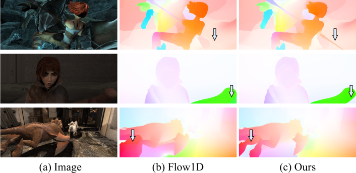
Figure 7: Qualitative comparisons on the Sintel test set. Our method can preserve more fine structure than Flow1D.

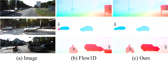
Figure 8: Qualitative comparisons on the KITTI test set. Our method performs well in large textureless regions.

Results of ablations are shown in Tab. 1. Following RAFT, the Base denotes the 2D lookup on target image feature in each iteration, and the lookup radius $r$ is set to 4. The proposed OC (orthogonal correlation) can greatly reduce memory consumption and speed up inference, especially on high-resolution images. The OC only indexes $(2r\!+\!1)\!\times\!2$ target feature in two 1D orthogonal directions for each pixel on the source feature. To complement information loss, we exploit OA (orthogonal attention) to propagate the feature information of the 2D space to the orthogonal space, which can significantly improve the overall performance at a negligible cost. To efficiently provide information of large displacements, we propose a new radius-distribution multi-scale lookup strategy, named RDMS. The propose OC+OA+RDMS, denoted as MeFlow, achieves the best performance.

Cost Volume	Method	Sintel (train, clean)
		EPE	EPE ($h$)	EPE ($v$)
$v$ attn, $h$ corr	Flow1D	3.10	1.66	2.12
	MeFlow	1.79	1.14	1.10
$h$ attn, $v$ corr	Flow1D	4.05	3.55	1.13
	MeFlow	1.79	1.37	0.85
concat both	Flow1D	1.98	1.48	0.94
	MeFlow	1.49	1.08	0.79

Table 5: Analysis on horizontal ($h$) and vertical ($v$) cost volumes. EPE ($h$) and EPE ($v$) represent the end-point-error of the horizontal and vertical flow component, respectively.

Method	Sintel (test, final)
	EPE	s0-10	s10-40	s40+
Flow1D	3.81	0.74	2.48	22.22
Ours	3.09	0.64 (14%$\uparrow$)	1.77 (29%$\uparrow$)	18.46(17%$\uparrow$)

Table 6: Comparisons with Flow1D in different ranges of optical flow regions. Our method performs better in large motion regions (s_0-10, s₄₀₊).

Method	Sintel (test)		KITTI (F1-all)
	Clean	Final	train	test
FlowNet2 [13]	4.16	5.74	(6.8)	11.48
LiteFlowNet2 [11]	3.48	4.69	(4.8)	7.74
PWC-Net+ [30]	3.45	4.60	(5.3)	7.72
HD3 [45]	4.79	4.67	(4.1)	6.55
IRR-PWC [12]	3.84	4.58	(5.3)	7.65
IRR-PWC-it [31]	2.19	3.55	-	5.73
VCN [43]	2.81	4.40	(4.1)	6.30
DICL [36]	2.12	3.44	(3.6)	6.31
MaskFlowNet [47]	2.52	4.17	-	6.10
RAFT [34]	1.61	2.86	(1.5)	5.10
GMA [14]	1.39	2.47	(1.2)	5.15
GMFlow [40]	1.74	2.90	-	9.32
GMFlow+ [41]	1.03	2.37	-	4.49
SKFlow [33]	1.28	2.23	(0.94)	4.84
FlowFormer [9]	1.18	2.36	(1.1)	4.87
DEQ-RAFT [1]	1.82	3.23	(1.4)	4.98
EMD-L [5]	1.32	2.51	-	4.51
SCV [15]	1.72	3.60	(2.1)	6.17
Flow1D [39]	2.24	3.81	(1.6)	6.27
MeFlow (Ours)	2.05	3.09	(1.6)	4.95

Table 7: Benchmark performance on Sintel and KITTI datasets. The numbers in parentheses are the results from fine-tuning the methods on the data.

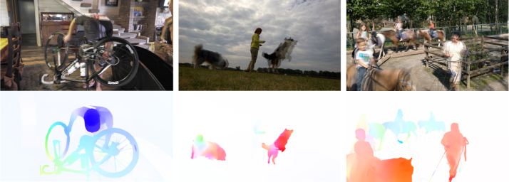
Figure 9: Optical flow prediction results on 4K ($2160\times 3840$) resolution images from DAVIS [23, 3] datasets. From top to bottom: overlapping images and optical flow results.

4.3 Comparison with Existing Methods

Comparison with existing cost volumes. We conduct comprehensive comparisons with existing representative cost volume construction methods to demonstrate the superiority of our local orthogonal cost volume method. Results are shown in Tab. 2. FlowNet2 [13] constructs a single-scale cost volume, PWC-Net [29] constructs a coarse-to-fine cost volume pyramid, RAFT [34] constructs an all-pairs 4D cost volume, and Flow1D [39] constructs two 3D cost volumes. We evaluate the cross-dataset generalization ability on Sintel and KITTI training sets and show benchmark results on KITTI. In this evaluation, our method achieves the best performance in terms of accuracy and memory consumption. In particular, our method outperforms PWC-Net by 49.5% and Flow1D by 21.1% on KITTI, and exhibits higher memory efficiency. For high-resolution $1080\times 1920$ images, our MeFlow can consume $6\times$ less memory than RAFT.

Comparison with memory-efficient methods. We compare our MeFlow with memory-efficient methods based on recurrent optimization, shown in Tab. 3. Our method outperforms SCV [15] and Flow1D [39] on KITTI. Our method is slightly inferior compared to DIP [49] in terms of accuracy but enjoys less memory consumption and inference time. Sequential ConvGRU in DIP is time-consuming, and our method yields a $2.4\times$ speedup than DIP for $1080\times 1920$ resolution images.

Comparison with accuracy-oriented methods. We compare our MeFlow with accuracy-oriented methods, shown in Tab. 4. Our method achieves competitive accuracy on the KITTI benchmark, and shows higher efficiency than these accuracy-oriented methods in terms of both memory consumption and inference speed. The superiority will be more significant for high-resolution images. For example, when the input image resolution is $1080\times 1920$, our method consumes $\mathbf{8\times}$ less memory than GMA [14] and SKFlow [33], and yields a $4.8\times$ speedup than GMFlow [40], $2.4\times$ speedup than SKFlow [33]. FlowFormer causes an out-of-memory error for $1080\times 1920$ resolution on our 24G GPU.

Analysis on horizontal and vertical cost volume. We decompose the orthogonal cost volume into horizontal cost volume ($v$ attn, $h$ corr) and vertical cost volume ($h$ attn, $v$ corr) and evaluate the corresponding performance, shown in Tab. 5. With only horizontal or vertical cost volume, our method still achieves comparable performance, which is even better than Flow1D [39] with both horizontal and vertical cost volumes. With the same cost volume setup, our method outperforms Flow1D by a large margin.

High-resolution performance. Our MeFlow can scale up well to very high-resolution images. As shown in Fig. 6, we show visual comparisons on the high-resolution ($1080\!\times\!1920$) DAVIS dataset. Our method achieves comparable results with RAFT while consuming $6\times$ less memory, and significantly better results than Flow1D while consuming similar memory. In Fig. 9, we also show visual results on 4K ($2160\!\times\!3840$) resolution images from DAVIS datasets. Our MeFlow can handle 4K images with only 5.4G memory usage. RAFT can not handle 4K images due to causing an out-of-memory error on our 24G GPU.

4.4 Benchmark Results

The results of our MeFlow on Sintel and KITTI benchmarks are shown in Tab. 7. Our method achieves comparable results with other methods. On Sintel and KITTI benchmark, our method is inferior to some accuracy-oriented methods such as SKFlow [33] and FlowFormer [9], but outperforms most existing methods such as PWC-Net+ [30], MaskFlowNet [47] and Flow1D [39]. Specially, our method outperforms the equally memory-efficient Flow1D by a large margin, e.g., exceeding Flow1D 21.1% on KITTI and 18.9% on Sintel (Final). We also show visual comparisons on the Sintel and KITTI test sets, shown in Fig. 7 and Fig. 8. Compared with Flow1D, our method can perform better in the fine structure and large textureless areas. Specially, Flow1D struggles to handle large motions since its two 3D cost volumes lose matching information for large displacements, as illustrated in Fig. 3 and Tab. 6. In contrast, our method can handle large motions (s_0-10, s₄₀₊) well.

5 Conclusion

The full 4D cost volume in RAFT and global matching in GMFlow achieve striking performance for optical flow estimation. However, their memory consumption grows quadratically with input resolution, making them impractical for high-resolution images. In this paper, we propose a novel local orthogonal cost volume that decomposes the 2D search space dynamically into two 1D orthogonal spaces by attention, enabling our method to scale well to high-resolution images. We further propose a new radius-distribution multi-scale lookup strategy to model the correspondences of large displacements. Our MeFlow achieves the highest memory efficiency among all methods and competitive accuracy compared to the state-of-the-art. We hope the proposed efficient local orthogonal cost volume will inspire future research on high-resolution optical flow estimation.

References

- Bai et al. [2022] Shaojie Bai, Zhengyang Geng, Yash Savani, and J Zico Kolter. Deep equilibrium optical flow estimation. In IEEE Conf. Comput. Vis. Pattern Recog., pages 620–630, 2022.
- Butler et al. [2012] Daniel J Butler, Jonas Wulff, Garrett B Stanley, and Michael J Black. A naturalistic open source movie for optical flow evaluation. In Eur. Conf. Comput. Vis., pages 611–625. Springer, 2012.
- Caelles et al. [2019] Sergi Caelles, Jordi Pont-Tuset, Federico Perazzi, Alberto Montes, Kevis-Kokitsi Maninis, and Luc Van Gool. The 2019 davis challenge on vos: Unsupervised multi-object segmentation. arXiv:1905.00737, 2019.
- Carion et al. [2020] Nicolas Carion, Francisco Massa, Gabriel Synnaeve, Nicolas Usunier, Alexander Kirillov, and Sergey Zagoruyko. End-to-end object detection with transformers. In Eur. Conf. Comput. Vis., pages 213–229. Springer, 2020.
- Deng et al. [2023] Changxing Deng, Ao Luo, Haibin Huang, Shaodan Ma, Jiangyu Liu, and Shuaicheng Liu. Explicit motion disentangling for efficient optical flow estimation. In Int. Conf. Comput. Vis., pages 9521–9530, 2023.
- Dosovitskiy et al. [2015] Alexey Dosovitskiy, Philipp Fischer, Eddy Ilg, Philip Hausser, Caner Hazirbas, Vladimir Golkov, Patrick Van Der Smagt, Daniel Cremers, and Thomas Brox. Flownet: Learning optical flow with convolutional networks. In Int. Conf. Comput. Vis., pages 2758–2766, 2015.
- Fu et al. [2019] Jun Fu, Jing Liu, Haijie Tian, Yong Li, Yongjun Bao, Zhiwei Fang, and Hanqing Lu. Dual attention network for scene segmentation. In IEEE Conf. Comput. Vis. Pattern Recog., pages 3146–3154, 2019.
- Huang et al. [2019] Zilong Huang, Xinggang Wang, Lichao Huang, Chang Huang, Yunchao Wei, and Wenyu Liu. Ccnet: Criss-cross attention for semantic segmentation. In Int. Conf. Comput. Vis., pages 603–612, 2019.
- Huang et al. [2022] Zhaoyang Huang, Xiaoyu Shi, Chao Zhang, Qiang Wang, Ka Chun Cheung, Hongwei Qin, Jifeng Dai, and Hongsheng Li. Flowformer: A transformer architecture for optical flow. In Eur. Conf. Comput. Vis., pages 668–685. Springer, 2022.
- [10] TW Hui, X Tang, and C Liteflownet Change Loy. A lightweight convolutional neural network for optical flow estimation. In IEEE Conf. Comput. Vis. Pattern Recog., pages 8981–8989.
- Hui et al. [2020] Tak-Wai Hui, Xiaoou Tang, and Chen Change Loy. A lightweight optical flow cnn—revisiting data fidelity and regularization. IEEE Trans. Pattern Anal. Mach. Intell., 43(8):2555–2569, 2020.
- Hur and Roth [2019] Junhwa Hur and Stefan Roth. Iterative residual refinement for joint optical flow and occlusion estimation. In IEEE Conf. Comput. Vis. Pattern Recog., pages 5754–5763, 2019.
- Ilg et al. [2017] Eddy Ilg, Nikolaus Mayer, Tonmoy Saikia, Margret Keuper, Alexey Dosovitskiy, and Thomas Brox. Flownet 2.0: Evolution of optical flow estimation with deep networks. In IEEE Conf. Comput. Vis. Pattern Recog., pages 2462–2470, 2017.
- Jiang et al. [2021a] Shihao Jiang, Dylan Campbell, Yao Lu, Hongdong Li, and Richard Hartley. Learning to estimate hidden motions with global motion aggregation. In Int. Conf. Comput. Vis., pages 9772–9781, 2021a.
- Jiang et al. [2021b] Shihao Jiang, Yao Lu, Hongdong Li, and Richard Hartley. Learning optical flow from a few matches. In IEEE Conf. Comput. Vis. Pattern Recog., pages 16592–16600, 2021b.
- Liu et al. [2021] Ze Liu, Yutong Lin, Yue Cao, Han Hu, Yixuan Wei, Zheng Zhang, Stephen Lin, and Baining Guo. Swin transformer: Hierarchical vision transformer using shifted windows. In Int. Conf. Comput. Vis., pages 10012–10022, 2021.
- Loshchilov and Hutter [2017] Ilya Loshchilov and Frank Hutter. Decoupled weight decay regularization. arXiv preprint arXiv:1711.05101, 2017.
- Luo et al. [2022a] Ao Luo, Fan Yang, Xin Li, and Shuaicheng Liu. Learning optical flow with kernel patch attention. In IEEE Conf. Comput. Vis. Pattern Recog., pages 8906–8915, 2022a.
- Luo et al. [2022b] Ao Luo, Fan Yang, Kunming Luo, Xin Li, Haoqiang Fan, and Shuaicheng Liu. Learning optical flow with adaptive graph reasoning. In AAAI, pages 1890–1898, 2022b.
- Luo et al. [2023] Ao Luo, Fan Yang, Xin Li, Lang Nie, Chunyu Lin, Haoqiang Fan, and Shuaicheng Liu. Gaflow: Incorporating gaussian attention into optical flow. In Int. Conf. Comput. Vis., pages 9642–9651, 2023.
- Mayer et al. [2016] Nikolaus Mayer, Eddy Ilg, Philip Hausser, Philipp Fischer, Daniel Cremers, Alexey Dosovitskiy, and Thomas Brox. A large dataset to train convolutional networks for disparity, optical flow, and scene flow estimation. In IEEE Conf. Comput. Vis. Pattern Recog., pages 4040–4048, 2016.
- Menze and Geiger [2015] Moritz Menze and Andreas Geiger. Object scene flow for autonomous vehicles. In IEEE Conf. Comput. Vis. Pattern Recog., pages 3061–3070, 2015.
- Pont-Tuset et al. [2017] Jordi Pont-Tuset, Federico Perazzi, Sergi Caelles, Pablo Arbeláez, Alexander Sorkine-Hornung, and Luc Van Gool. The 2017 davis challenge on video object segmentation. arXiv:1704.00675, 2017.
- Sevilla-Lara et al. [2019] Laura Sevilla-Lara, Yiyi Liao, Fatma Güney, Varun Jampani, Andreas Geiger, and Michael J Black. On the integration of optical flow and action recognition. In German conference on pattern recognition, pages 281–297. Springer, 2019.
- Shi et al. [2023a] Xiaoyu Shi, Zhaoyang Huang, Weikang Bian, Dasong Li, Manyuan Zhang, Ka Chun Cheung, Simon See, Hongwei Qin, Jifeng Dai, and Hongsheng Li. Videoflow: Exploiting temporal cues for multi-frame optical flow estimation. arXiv preprint arXiv:2303.08340, 2023a.
- Shi et al. [2023b] Xiaoyu Shi, Zhaoyang Huang, Dasong Li, Manyuan Zhang, Ka Chun Cheung, Simon See, Hongwei Qin, Jifeng Dai, and Hongsheng Li. Flowformer++: Masked cost volume autoencoding for pretraining optical flow estimation. In IEEE Conf. Comput. Vis. Pattern Recog., pages 1599–1610, 2023b.
- Sui et al. [2022] Xiuchao Sui, Shaohua Li, Xue Geng, Yan Wu, Xinxing Xu, Yong Liu, Rick Goh, and Hongyuan Zhu. Craft: Cross-attentional flow transformer for robust optical flow. In IEEE Conf. Comput. Vis. Pattern Recog., pages 17602–17611, 2022.
- Sun et al. [2018a] Chen Sun, Abhinav Shrivastava, Carl Vondrick, Kevin Murphy, Rahul Sukthankar, and Cordelia Schmid. Actor-centric relation network. In Eur. Conf. Comput. Vis., pages 318–334, 2018a.
- Sun et al. [2018b] Deqing Sun, Xiaodong Yang, Ming-Yu Liu, and Jan Kautz. Pwc-net: Cnns for optical flow using pyramid, warping, and cost volume. In IEEE Conf. Comput. Vis. Pattern Recog., pages 8934–8943, 2018b.
- Sun et al. [2019] Deqing Sun, Xiaodong Yang, Ming-Yu Liu, and Jan Kautz. Models matter, so does training: An empirical study of cnns for optical flow estimation. IEEE Trans. Pattern Anal. Mach. Intell., 42(6):1408–1423, 2019.
- Sun et al. [2022a] Deqing Sun, Charles Herrmann, Fitsum Reda, Michael Rubinstein, David J Fleet, and William T Freeman. Disentangling architecture and training for optical flow. In Eur. Conf. Comput. Vis., pages 165–182. Springer, 2022a.
- Sun et al. [2021] Jiaming Sun, Zehong Shen, Yuang Wang, Hujun Bao, and Xiaowei Zhou. Loftr: Detector-free local feature matching with transformers. In IEEE Conf. Comput. Vis. Pattern Recog., pages 8922–8931, 2021.
- Sun et al. [2022b] Shangkun Sun, Yuanqi Chen, Yu Zhu, Guodong Guo, and Ge Li. Skflow: Learning optical flow with super kernels. arXiv preprint arXiv:2205.14623, 2022b.
- Teed and Deng [2020] Zachary Teed and Jia Deng. Raft: Recurrent all-pairs field transforms for optical flow. In Eur. Conf. Comput. Vis., pages 402–419. Springer, 2020.
- Wang et al. [2020a] Huiyu Wang, Yukun Zhu, Bradley Green, Hartwig Adam, Alan Yuille, and Liang-Chieh Chen. Axial-deeplab: Stand-alone axial-attention for panoptic segmentation. In Eur. Conf. Comput. Vis., pages 108–126. Springer, 2020a.
- Wang et al. [2020b] Jianyuan Wang, Yiran Zhong, Yuchao Dai, Kaihao Zhang, Pan Ji, and Hongdong Li. Displacement-invariant matching cost learning for accurate optical flow estimation. Adv. Neural Inform. Process. Syst., 33:15220–15231, 2020b.
- Xu et al. [2022a] Gangwei Xu, Junda Cheng, Peng Guo, and Xin Yang. Attention concatenation volume for accurate and efficient stereo matching. In IEEE Conf. Comput. Vis. Pattern Recog., pages 12981–12990, 2022a.
- Xu et al. [2023a] Gangwei Xu, Yun Wang, Junda Cheng, Jinhui Tang, and Xin Yang. Accurate and efficient stereo matching via attention concatenation volume. IEEE Trans. Pattern Anal. Mach. Intell., 2023a.
- Xu et al. [2021] Haofei Xu, Jiaolong Yang, Jianfei Cai, Juyong Zhang, and Xin Tong. High-resolution optical flow from 1d attention and correlation. In Int. Conf. Comput. Vis., pages 10498–10507, 2021.
- Xu et al. [2022b] Haofei Xu, Jing Zhang, Jianfei Cai, Hamid Rezatofighi, and Dacheng Tao. Gmflow: Learning optical flow via global matching. In IEEE Conf. Comput. Vis. Pattern Recog., pages 8121–8130, 2022b.
- Xu et al. [2023b] Haofei Xu, Jing Zhang, Jianfei Cai, Hamid Rezatofighi, Fisher Yu, Dacheng Tao, and Andreas Geiger. Unifying flow, stereo and depth estimation. IEEE Trans. Pattern Anal. Mach. Intell., 2023b.
- Yang et al. [2021] Charig Yang, Hala Lamdouar, Erika Lu, Andrew Zisserman, and Weidi Xie. Self-supervised video object segmentation by motion grouping. In Int. Conf. Comput. Vis., pages 7177–7188, 2021.
- Yang and Ramanan [2019] Gengshan Yang and Deva Ramanan. Volumetric correspondence networks for optical flow. Adv. Neural Inform. Process. Syst., 32, 2019.
- Yang and Ramanan [2021] Gengshan Yang and Deva Ramanan. Learning to segment rigid motions from two frames. In IEEE Conf. Comput. Vis. Pattern Recog., pages 1266–1275, 2021.
- Yin et al. [2019] Zhichao Yin, Trevor Darrell, and Fisher Yu. Hierarchical discrete distribution decomposition for match density estimation. In IEEE Conf. Comput. Vis. Pattern Recog., pages 6044–6053, 2019.
- Zhang et al. [2021] Feihu Zhang, Oliver J Woodford, Victor Adrian Prisacariu, and Philip HS Torr. Separable flow: Learning motion cost volumes for optical flow estimation. In Int. Conf. Comput. Vis., pages 10807–10817, 2021.
- Zhao et al. [2020] Shengyu Zhao, Yilun Sheng, Yue Dong, Eric I Chang, Yan Xu, et al. Maskflownet: Asymmetric feature matching with learnable occlusion mask. In IEEE Conf. Comput. Vis. Pattern Recog., pages 6278–6287, 2020.
- Zhao et al. [2022] Shiyu Zhao, Long Zhao, Zhixing Zhang, Enyu Zhou, and Dimitris Metaxas. Global matching with overlapping attention for optical flow estimation. In IEEE Conf. Comput. Vis. Pattern Recog., pages 17592–17601, 2022.
- Zheng et al. [2022] Zihua Zheng, Ni Nie, Zhi Ling, Pengfei Xiong, Jiangyu Liu, Hao Wang, and Jiankun Li. Dip: Deep inverse patchmatch for high-resolution optical flow. In IEEE Conf. Comput. Vis. Pattern Recog., pages 8925–8934, 2022.