Computation of the optimal error exponent function for fixed-length lossy source coding in discrete memoryless sources

Abstract

The error exponent of fixed-length lossy source coding was established by Marton. Ahlswede showed that this exponent can be discontinuous at a rate $R$, depending on the source distribution $P$ and the distortion measure $d(x,y)$. The reason for the discontinuity in the error exponent is that there exists a distortion measure $d(x,y)$ and a distortion level $\Delta$ such that the rate-distortion function $R(\Delta|P)$ is neither concave nor quasi-concave with respect to $P$. Arimoto’s algorithm for computing the error exponent in lossy source coding is based on Blahut’s parametric representation of the error exponent. However, Blahut’s parametric representation is a lower convex envelope of Marton’s exponent, and the two do not generally agree. A major contribution of this paper is to provide a parametric representation that perfectly matches the inverse function of Marton’s exponent, thereby preventing the problems arising from the above-mentioned non-concavity of $R(\Delta|P)$. For fixed parameters, an optimal distribution can be obtained using Arimoto’s algorithm. By performing a nonconvex optimization over the parameters, the inverse function of Marton’s exponent is obtained.

I Introduction

The rate-distortion function for an independent binary source $P(0)=p$ and $P(1)=1-p$ with Hamming distortion measure is given by [1, Chapter 10.3]

$$R(\Delta|P)=\begin{cases}h(p)-h(\Delta),&0\leq\Delta\leq\min\{p,1-p\},\\ 0,&\Delta>\min\{p,1-p\},\end{cases}$$ (1)

where $h(p)=-p\log p-(1-p)\log(1-p)$ is the binary entropy function. Because (1) is quasi-concave in $P$, one might expect that so is in general. In [2], Ahlswede disproved this conjecture by giving a counterexample that for a fixed $\Delta$, $R(\Delta|P)$ as a function $P$ has a local maximum that is different from the global maximum. As a consequence, he showed that Marton’s optimal error exponent of fixed-length lossy source coding [3] can be discontinuous at some rate $R$ for a fixed $\Delta$ and $P$.

For a given information source, the rate-distortion function is usually not explicitly expressed, and is defined as the solution to a certain optimization problem. An algorithm for elegantly solving this optimization problem is given by Blahut [4] and, together with Arimoto’s algorithm [5] for computing the channel capacity of a discrete memoryless channel, is called the Arimoto-Blahut algorithm. Arimoto also gave an algorithm for computing the error exponent for lossy source coding [6], but his algorithm is based on Blahut’s suboptimal error exponent. Since Marton’s exponent is defined as a nonconvex optimization problem, standard convex optimization techniques are not straightforwardly applicable to compute it. An efficient algorithm for computing Marton’s exponent has been an open problem since Arimoto stated it in [6].

The main contribution of this paper is that we establish a parametric expression with two parameters that perfectly matches the inverse function of Marton’s exponent. When the parameters are fixed, such an expression involves only convex optimization, which can be computed efficiently by the Arimoto algorithm [6]. This implies that a nonconvex optimization over probability distributions is transformed into a nonconvex optimization over two parameters with a convex optimization over probability distributions. Using Ahlswede’s counterexample, we show that the parametric expression allows us to correctly draw the inverse function of Marton’s exponent.

II Preliminary

II-A The error exponent for lossy source coding

We begin with definitions of the rate-distortion function and error exponent of fixed-length lossy source coding. Consider a discrete memoryless source (DMS) with a source alphabet $\mathcal{X}$ and a reconstruction alphabet $\mathcal{Y}$. Assume $\mathcal{X}$ and $\mathcal{Y}$ are finite sets. The set of probability distributions on $\mathcal{X}$ is denoted by $\mathcal{P(X)}$. Fix a probability distribution on $\mathcal{X}$, denoted by $P\in\mathcal{P(X)}$. Let a letter-wise distortion measure denoted by $d(x,y)\geq 0$. Then, the rate-distortion function is given by

$$R(\Delta|P)=\min_{\genfrac{}{}{0.0pt}{}{q_{Y|X}\in\mathcal{P(Y|X)}:}{\mathrm{E}[d(X,Y)]\leq\Delta}}I(P,q_{Y|X}),$$ (2)

where

$$I(P,q_{Y|X})$$

$$=\sum_{x\in\mathcal{X}}\sum_{y\in\mathcal{Y}}P(x)q_{Y|X}(y|x)\log\frac{q_{Y|X}(y|x)}{\sum_{x^{\prime}\in\mathcal{X}}P(x^{\prime})q_{Y|X}(y|x^{\prime})}$$

is the mutual information between the source and its reconstruction, $\mathcal{P(Y|X)}$ is the set of conditional probability distributions on $\mathcal{Y}$ given $\mathcal{X}$. Here the expectation of $d(X,Y)$ is taken over the joint probability distributions $P(x)\cdot q_{Y|X}(y|x)$. We have $R(\Delta|P)=0$ if $\Delta\geq\Delta_{\max}:={\min_{y}}\sum_{x\in\mathcal{X}}P(x)d(x,y)$.

Marton proved that the following function is the optimal error exponent [3]. For a fixed $\Delta\in[0,\Delta_{\max}]$, her exponent is defined by

$$E_{\rm M}(R|\Delta,P)=\min_{\genfrac{}{}{0.0pt}{}{q_{X}\in\mathcal{P(X)}:}{R(\Delta|q_{X})\geq R}}D(q_{X}\|P)$$ (3)

for $0\leq R\leq R_{\max}(\Delta):=\max_{q_{X}\in\mathcal{P(X)}}R(\Delta|q_{X})$, where $D(\cdot\|\cdot)$ denotes the relative entropy. From its definition, it is clear that $E_{\rm M}(R|\Delta,P)$ satisfies the following properties.

Property 1

1. $E_{\rm M}(R|\Delta,P)=0$ if $R\leq R(\Delta|P)$.

2. For fixed $\Delta\geq 0$ and $P\in\mathcal{P(X)}$, $E_{\rm M}(R|\Delta,P)$ is a monotone non-decreasing function of $R\in[0,R_{\max}(\Delta)]$.

Arimoto’s computation algorithm for error exponent [6] is based on the parametric expression of Blahut’s exponent [7], defined by

$$E_{\rm B}(R|\Delta,P)$$

$$=\sup_{\rho\geq 0}\bigg{\{}\rho R-\sup_{\nu\geq 0}\Big{[}\max_{p_{Y}}E_{0,\rm s}^{(\rho,\nu)}(p_{Y}|P)-\rho\nu\Delta\Big{]}\bigg{\}}$$ (4)

for $0\leq\Delta\leq\Delta_{\rm max}$ and $0\leq R\leq R_{\max}(\Delta)$, where

$$E_{0,\rm s}^{(\rho,\nu)}(p_{Y}|P)$$

$$=-\log\sum_{x\in\mathcal{P(X)}}P(x)\bigg{\{}\sum_{y\in\mathcal{Y}}p_{Y}(y){\rm e}^{-\nu d(x,y)}\bigg{\}}^{-\rho}.$$ (5)

From (4), it is observed that $\rho R-\sup_{\nu\geq 0}\Big{[}\max_{p_{Y}}E_{0,\rm s}^{(\rho,\nu)}(p_{Y}|P)-\rho\nu\Delta\Big{]}$ is the supporting line to the curve $E_{\rm B}(R|\Delta,P)$ with slope $\rho$ and thus $E_{\rm B}(R|\Delta,P)$ is a convex function of $R$.

Remark 1

In the expression of Blahut’s exponent (4), $\max_{p_{Y}}E_{0,\rm s}^{(\rho,\nu)}(p_{Y}|P)$ is not necessarily concave in $\nu$ for fixed $\rho$ and $P$. Hence, the computation of Blahut’s exponent requires nonlinear optimization over $\nu$. See Section IV for a graph of an example of $\max_{p_{Y}}E_{0,\rm s}^{(\rho,\nu)}(p_{Y}|P)-\rho\nu\Delta$ with two local maxima.

An important relation between $E_{\rm M}(R|\Delta,P)$ and $E_{\rm B}(R|\Delta,P)$ is stated as follows:

Lemma 1

For any $P\in\mathcal{P(X)}$, distortion measure $d(x,y)$, $R\geq 0$, and $\Delta\geq 0$, $E_{\rm B}(R|\Delta,P)$ is a lower convex envelope of $E_{\rm M}(R|\Delta,P)$.

The proof of Lemma 1 is given in Section V-B.

To the best of the author’s knowledge, any computation method for Marton’s exponent has not been established. The reason why it is difficult to derive an algorithm for computing Marton’s exponent is that for a given distortion measure $d(x,y)$, $R(\Delta|P)$ is not necessarily concave with respect to (w.r.t.) $P$. Hence, the feasible region $\{q_{X}\in\mathcal{P(X)}\colon R(\Delta|q_{X})\geq R\}$ in (3) is not necessarily convex.

According to the standard approach to solving the optimization problem with equality and inequality constraints, we can introduce the Lagrange multipliers for the constraints and consider an unconstrained optimization. The Lagrange dual of the primal problem of (3) is given by

$$\sup_{\rho\geq 0}\min_{q_{X}\in\mathcal{P(X)}}\{D(q_{X}\|P)+\rho[R-R(\Delta|q_{X})]\}.$$ (6)

However, there may be a gap between the primal problem (3) and (6) since $R(\Delta|q_{X})$ is not necessarily concave in $q_{X}$. To circumvent this issue, we use the inverse function of Marton’s exponent. In the next subsection, we give the definition and the basic property of such an inverse function.

II-B Inverse Function of Marton’s Exponent

The inverse function of Marton’s error exponent is expressed by the following formula.

Definition 1

For $E\geq 0$ and $\Delta\geq 0$, we define

$$R_{\rm M}(E|\Delta,P)=\max_{\genfrac{}{}{0.0pt}{}{q_{X}\in\mathcal{P(X)}:}{D(q_{X}\|P)\leq E}}R(\Delta|q_{X}).$$ (7)

The idea of analyzing the inverse function of the error exponent was first introduced by Haroutunian et al. [9, 10]. They defined the rate-reliability-distortion function as the minimum rate at which the encoded messages can be reconstructed by the decoder with exponentially decreasing probabilities of error. They proved that the optimal rate-reliability-distortion function is given by (7).

Let us discuss some basic properties of the rate-reliability-distortion function $R_{\rm M}(E|\Delta,P)$. Fix $\Delta>0$ and $P\in\mathcal{P(X)}$. Hereafter, we assume that the distortion measure $d(x,y)$ satisfies

$$\max_{x\in\mathcal{X}}\min_{y\in\mathcal{Y}}d(x,y)=0,$$ (8)

$$d_{\rm max} =\max_{(x,y)\in\mathcal{X\times Y}}d(x,y)<\infty.$$ (9)

This assumption ensures Item d) of Property 2 given below.

Let the local maxima of $R(\Delta|q_{X})$ w.r.t. $q_{X}\in\mathcal{P(X)}$ denoted by $R_{1}\leq R_{2}\leq\cdots\leq R_{m}$. The largest local maximum $R_{m}=R_{\rm max}(\Delta)$ is the global maximum of $R(\Delta|q_{X})$. Let $\mathcal{Q}_{i}$, $i=1,2,\ldots,m$, be a subset of $\mathcal{P(X)}$ in which every distribution in $\mathcal{Q}_{i}$ achieves the local maximum $R_{i}$. That is, for each $i$, there exists an $\epsilon>0$ such that for any $q_{X}\in\mathcal{Q}_{i}$, $R(\Delta|q_{X})=R_{i}$ holds and for any $p_{X}$ with $\lVert p_{X}-q_{X}\rVert\leq\epsilon$ satisfies $R(\Delta|p_{X})\leq R_{i}$. Define $E_{i}=\min_{q_{X}\in\mathcal{Q}_{i}}D(q_{X}\|P)$ and denote $E_{m}$ by $E_{\rm max}$.

The function $R_{\rm M}(E|\Delta,P)$ satisfies the following basic properties:

Property 2

1. $R_{\rm M}(0|\Delta,P)=R(\Delta|P)$ holds.

2. $R_{\rm M}(E|\Delta,P)=R_{\max}(\Delta)$ for $E\geq E_{\rm max}$.

3. $R_{\rm M}(E|\Delta,P)$ is a monotonically non-decreasing function of $E\geq 0$ for fixed $\Delta\geq 0$ and $P$.

4. $R_{\rm M}(E|\Delta,P)$ is a continuous function of $E\geq 0$ for fixed $\Delta\geq 0$

Proof: Property 2 a) holds since $D(q_{X}\|P)=0$ implies $q_{X}=P$. Property 2 b) holds because if $E\geq E_{\rm max}$, we can choose an optimal $q_{X}$ that achieves the global maximum of $R(\Delta|q_{X})$. For Property 2 c), the monotonicity is obvious from the definition. See Section V-A for the proof of Property 2 d).

∎

Here, we divide the optimal distribution $q_{X}^{*}$ of the optimization problem $R_{\rm M}(E|\Delta,P)$ defined by (7) into two cases: one is achieved at the boundary and the other at an interior point of the feasible region. The optimal distribution $q_{X}^{*}$ satisfies $D(q_{X}^{*}\|P)=E$ in the former case and $D(q_{X}^{*}\|P)<E$ in the latter case. To distinguish between these two cases more clearly, we introduce the following function.

$$\widetilde{R}_{\rm M}(E|\Delta,P)=\max_{\genfrac{}{}{0.0pt}{}{q_{X}\in\mathcal{P(X)}:}{D(q_{X}\|P)=E}}R(\Delta|q_{X}).$$ (10)

For avoiding the set $\{q_{X}\in\mathcal{P(X)}:D(q_{X}\|P)=E\}$ to be empty, $\widetilde{R}_{\rm M}(E|\Delta,P)$ is defined for $E\in[0,E^{*}]$, where $E^{*}=-\log\min_{\genfrac{}{}{0.0pt}{}{x\in\mathcal{X}:}{P(x)>0}}P(x)$.

We have the following lemma.

Lemma 2

For $E\geq 0$, we have

$$R_{\rm M}(E|\Delta,P)=\max_{E^{\prime}\leq E}\widetilde{R}_{\rm M}(E^{\prime}|\Delta,P).$$ (11)

See Section V-B for the proof.

Consider an example when $m=4$ and $E_{1}<E_{3}<E_{2}<E_{4}$. Assume that all the local maxima $R_{i}$ are achieved by unique $q_{X}$’s so that $\mathcal{Q}_{i}=\{q_{X}^{(i)}\}$, $i=1,\ldots,m$ are singleton sets. Then, we have $E_{i}=D(q_{X}^{(i)}\|P)$. A sketch of $R_{\rm M}(E|\Delta,P)$ of this case is shown in Fig. 1, where $\widetilde{R}_{\rm M}(E|\Delta,P)$ is also shown to aid understanding. It follows from (11) that the graph of $R_{\rm M}(E|\Delta,P)$ is flat with zero slope if $\widetilde{R}_{\rm M}(E|\Delta,P)<R_{\rm M}(E|\Delta,P)$ holds and this occurs when $R_{\rm M}(E|\Delta,P)$ is attained by an interior point of the feasible region $\{q_{X}\in\mathcal{P(X)}:D(q_{X}||P)\leq E\}$.

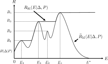
Figure 1: A graph of $R_{\rm M}(E|\Delta,P)$ (bold line) with the help of $\widetilde{R}_{\rm M}(E|\Delta,P)$ (dashed line).

The continuity property is an obvious advantage of treating with $R_{\rm M}(E|\Delta,P)$ instead of $E_{\rm M}(R|\Delta,P)$. The reason is that $E_{\rm M}(R|\Delta,P)$ may have a jump discontinuity at some $R$.

III Main Result

The main contribution of this paper is the establishment of a computation method for Marton’s exponent. Its derivation consists of three steps.

III-1 A parametric expression for the rate-distortion function

The function $R_{\rm M}(E|\Delta,P)$ is much easier to analyze than $E_{\rm M}(R|\Delta,P)$ because the feasible region in the right-hand side of (7) is convex. In (7), however, the objective function is the rate-distortion function, which is not necessarily convex. To circumvent this issue, we use the following parametric expression of $R(\Delta|q_{X})$. This is the first step.

Lemma 3

We have

$$R(\Delta|q_{X})=\sup_{\nu\geq 0}\Big{[}-\nu\Delta$$

$$\hskip 22.76219pt+\min_{p_{Y}\in\mathcal{P(Y)}}-\sum_{x}q_{X}(x)\log\sum_{y}p_{Y}(y)\mathrm{e}^{-\nu d(x,y)}\Big{]}.$$ (12)

One can refer [11, Corollary 8.5] for the proof.

We should mention that (12) is related to an important notion called the $d$-tilted information density [12], although this relation is not used in this paper. Denote the $\nu$ and $p_{Y}$ that attains (12) by $\nu^{*}$ and $p_{Y}^{*}$. Then,

$$\jmath_{X}(x,d):=-\log\sum_{y}p_{Y}^{*}(y){\rm e}^{-\nu^{*}(d(x,y)-\Delta)}$$ (13)

is called $d$-tilted information density and we observe that $R(\Delta|q_{X})={\rm E}_{q_{X}}[\jmath_{X}(X,d)]$ holds.

III-2 Minimax theorem

We substitute (12) into (7). Then, except for the maximization over $\nu\geq 0$, we have to evaluate the quantity defined by

$$\max_{\genfrac{}{}{0.0pt}{}{q_{X}\in\mathcal{P(X)}:}{D(q_{X}\|P)\leq E}}\min_{p_{Y}\in\mathcal{P(Y)}}-\sum_{x}q_{X}(x)\log\sum_{y}p_{Y}(y)\mathrm{e}^{-\nu d(x,y)}.$$ (14)

The second step is the exchange of the order of max and min in (14). For deriving an algorithm for computing $R_{\rm M}(E|\Delta,P)$, the saddle point (14) should be transformed into minimization or maximization problems. In order to derive such an expression, we exchange the order of maximization w.r.t. $q_{X}$ and minimization w.r.t. $p_{Y}$. The following lemma is essential for deriving the exact parametric expression for the inverse function of the error exponent.

Lemma 4

For any $E\geq 0$ and $\nu\geq 0$, we have

$$\max_{\genfrac{}{}{0.0pt}{}{q_{X}\in\mathcal{P(X)}:}{D(q_{X}\|P)\leq E}}\min_{p_{Y}\in\mathcal{P(Y)}}-\sum_{x}q_{X}(x)\log\sum_{y}p_{Y}(y)\mathrm{e}^{-\nu d(x,y)}$$

$$=\min_{p_{Y}\in\mathcal{P(Y)}}\max_{\genfrac{}{}{0.0pt}{}{q_{X}\in\mathcal{P(X)}:}{D(q_{X}\|P)\leq E}}-\sum_{x}q_{X}(x)\log\sum_{y}p_{Y}(y){\rm e}^{-\nu d(x,y)}$$ (15)

The validity of this exchange relies on Sion’s minimax theorem [13].

Theorem 1 (Sion [13])

Let $\mathcal{P}$ and $\mathcal{Q}$ be convex, compact spaces, and $f(p,q)$ a function on $\mathcal{P\times Q}$. If $f(p,q)$ is lower semicontinuous and quasi-convex on $p\in\mathcal{P}$ for any fixed $q\in\mathcal{Q}$ and $f(p,q)$ is upper semicontinuous and quasi-concave in $q\in\mathcal{Q}$ for any fixed $p\in\mathcal{P}$, then

$$\inf_{p\in\mathcal{P}}\sup_{q\in\mathcal{Q}}f(p,q)=\sup_{q\in\mathcal{Q}}\inf_{p\in\mathcal{P}}f(p,q).$$ (16)

Proof of Lemma 4: As stated above, the objective function of (14) is linear in $q_{X}$ and convex in $p_{Y}$. The set $\{q_{X}\in\mathcal{P(X)}:D(q_{X}\|P)\leq E\}$ is convex because $D(q_{X}\|P)$ is convex in $q_{X}$. Hence, we can apply Theorem 1 to (14). ∎

III-3 The second Lagrange multiplier

Next, we define the following functions:

Definition 2

For $\mu\geq 0,\nu\geq 0$, $p_{Y}\in\mathcal{P(Y)}$, and $P\in\mathcal{P(X)}$, we define

$$G^{(\nu)}(E,p_{Y}|P)$$

$$=\max_{\genfrac{}{}{0.0pt}{}{q_{X}\in\mathcal{P(X)}:}{D(q_{X}\|P)\leq E}}-\sum_{x}q_{X}(x)\log\sum_{y}p_{Y}(y){\rm e}^{-\nu d(x,y)},$$ (17)

$$G^{(\mu,\nu)}(p_{Y}|P)=\max_{q_{X}\in\mathcal{P(Y)}}\bigg{[}-\mu D(q_{X}\|P)$$

$$\hskip 22.76219pt-\sum_{x}q_{X}(x)\log\sum_{y}p_{Y}(y)\mathrm{e}^{-\nu d(x,y)}\bigg{]},$$ (18)

$$G^{(\mu,\nu)}(P)=\min_{p_{Y}\in\mathcal{P(Y)}}G^{(\mu,\nu)}(p_{Y}|P).$$ (19)

The last step is to transform (17), which is a constrained maximization, into an unconstrained maximization by introducing a Lagrange multiplier. For this purpose, we have defined (18). Then, (18) is explicitly obtained as follows:

Lemma 5

For $\mu,\nu\geq 0$, $p_{Y}\in\mathcal{P(Y)}$, and $P\in\mathcal{P(X)}$, we have

$$G^{(\mu,\nu)}(p_{Y}|P)$$

$$=\begin{cases}\mu\log\sum_{x}P(x)\left\{\sum_{y}p_{Y}(y)\mathrm{e}^{-\nu d(x,y)}\right\}^{-1/\mu}&\text{ if }\mu>0,\\ -\log\min_{x}\sum_{y}p_{Y}(y)\mathrm{e}^{-\nu d(x,y)}&\text{ if }\mu=0.\end{cases}$$ (20)

We have the following lemma.

Lemma 6

For $\nu\geq 0,E\geq 0,p_{Y}\in\mathcal{P(Y)}$, and $P\in\mathcal{P(X)}$, we have

$$G^{(\nu)}(E,p_{Y}|P)=\inf_{\mu\geq 0}\{\mu E+G^{(\mu,\nu)}(p_{Y}|P)\}.$$ (21)

The proofs of Lemmas 5 and 6 appear in Section V-B.

Eq. (21) is a parametric expression for (17). Finally, we obtain the following theorem.

Theorem 2

For any $P\in\mathcal{P(X)}$, $E\geq 0$, and $0\leq\Delta\leq\Delta_{\max}$, we have

$$R_{\rm M}(E|\Delta,P)=\sup_{\nu\geq 0}\inf_{\mu\geq 0}\left[-\nu\Delta+\mu E+G^{(\mu,\nu)}(P)\right].$$ (22)

Eq. (22) is valuable because it is an equation that is in perfect agreement with the inverse function of Marton’s optimal error exponent. To the best of our knowledge, such an exact parametric expression has not been known before.

Proof of Theorem 2: We have

$$R_{\rm M}(E|\Delta,P)$$

$$\stackrel{{\scriptstyle\rm(a)}}{{=}}\max_{\genfrac{}{}{0.0pt}{}{q_{X}\in\mathcal{P(X)}:}{D(q_{X}\|P)\leq E}}\sup_{\nu\geq 0}\Big{[}-\nu\Delta$$

$$\hskip 22.76219pt+\min_{p_{Y}\in\mathcal{P(Y)}}-\sum_{x}q_{X}(x)\log\sum_{y}p_{Y}(y)\mathrm{e}^{-\nu d(x,y)}\Big{]}$$

$$\stackrel{{\scriptstyle\rm(b)}}{{=}}\sup_{\nu\geq 0}\min_{p_{Y}\in\mathcal{P(Y)}}\max_{\genfrac{}{}{0.0pt}{}{q_{X}\in\mathcal{P(X)}:}{D(q_{X}\|P)\leq E}}\Big{[}-\nu\Delta$$

$$\hskip 22.76219pt-\sum_{x}q_{X}(x)\log\sum_{y}p_{Y}(y)\mathrm{e}^{-\nu d(x,y)}\Big{]}$$

$$\stackrel{{\scriptstyle\rm(c)}}{{=}}\sup_{\nu\geq 0}\min_{p_{Y}\in\mathcal{P(Y)}}\Big{[}-\nu\Delta+G^{(\nu)}(E,p_{Y}|P)\Big{]}$$

$$\stackrel{{\scriptstyle\rm(d)}}{{=}}\sup_{\nu\geq 0}\min_{p_{Y}\in\mathcal{P(Y)}}\Big{[}-\nu\Delta+\inf_{\mu\geq 0}\big{\{}\mu E+G^{(\mu,\nu)}(q_{Y}|P)\big{\}}\Big{]}$$

$$\stackrel{{\scriptstyle\rm(e)}}{{=}}\sup_{\nu\geq 0}\inf_{\mu\geq 0}\min_{p_{Y}\in\mathcal{P(Y)}}\Big{[}-\nu\Delta+\mu E+G^{(\mu,\nu)}(q_{Y}|P)\Big{]}$$

$$\stackrel{{\scriptstyle\rm(f)}}{{=}}\sup_{\nu\geq 0}\inf_{\mu\geq 0}\Big{[}-\nu\Delta+\mu E+G^{(\mu,\nu)}(P)\Big{]}.$$ (23)

Step (a) follows from Lemma 3, Step (b) follows from Lemma 4, Step (c) follows from Eq.(17), Step (d) follows from Eq.(21), Step (e) holds because the inf and min operations are interchangeable, and Step (f) follows from Eq.(19). ∎

Remark 2

The minimax theorem in Lemma 4 was the key step and the order of the above four steps is of crucial importance. From (7), we can define the Lagrange dual of $R_{\rm M}(E|\Delta,P)$ as

$$\hat{R}_{\rm M}(E|\Delta,P)$$

$$=\inf_{\mu\geq 0}\left\{\max_{q_{X}\in\mathcal{P(X)}:}[R(\Delta|q_{X})-\mu D(q_{X}\|P)]+\mu E\right\}.$$ (24)

However, the duality gap defined by $\hat{R}_{\rm M}(E|\Delta,P)-R_{\rm M}(E|\Delta,P)$ may be strictly positive, because of the nonconvex property of $R(\Delta|q_{X})$. The formulation (24) only leads to a suboptimal exponent. In fact, from (24), we have

$$\hat{R}_{\rm M}(E|\Delta,P)$$

$$=\inf_{\mu\geq 0}\left\{\sup_{\nu\geq 0}\left[G^{(\mu,\nu)}(P)-\nu\Delta\right]+\mu E\right\}.$$ (25)

The derivation can be done in a similar way to the proof of Theorem 2. Comparing (23) and (25) shows that the duality gap is represented by the order of the inf and sup operations in the parametric expressions.

Note that $G^{(\mu,\nu)}(p_{Y}|P)$ for $\mu>0$ in (20) is equal to (5) with $\rho=1/\mu$ multiplied by $-\mu$. Therefore, $\min_{p_{Y}}G^{(\mu,\nu)}(p_{Y}|P)$ is computed by Arimoto’s algorithm [6] with $\rho=1/\mu$ if $\mu>0$. If $\mu=0$, minimization of $G^{(\mu,\nu)}(p_{Y}|P)$ reduces to the following linear programming problem:

maximize $$c$$ (26)

subject to $$\sum_{y}p_{Y}(y)\mathrm{e}^{-\nu_{j}d(x,y)}\geq c,\quad^{\forall}x\in\mathcal{X},$$ (27)

$$p_{Y}(y)\geq 0,$$ (28)

$$\sum_{y\in\mathcal{P(Y)}}p_{Y}(y)=1,$$ (29)

where variables are $q_{Y}(y)$ and $c$. There are many solvers for linear programming. Their details are beyond the scope of this paper. The proposed algorithm is given in Algorithm 1 and Arimoto’s algorithm [6], which is used as a subroutine in Algorithm 1, is shown in Algorithm 2.

Algorithm 1 Proposed algorithm for computing the inverse function of the optimal error exponent in lossy source coding

1:procedure Computation_Inverse_of_Error_Exponent ($P,d,\Delta$)

2:     Set $N,M,K$ and $\varDelta\mu,\varDelta\nu,\varDelta E$ according to the precision.

3:     for $k=0$ to $K-1$ do

4:         $E_{k}=k(\varDelta E)$

5:         for $j=0$ to $M-1$ do

6:              $\nu_{j}=j(\varDelta\nu)$

7:              Solve (26) to (29) to obtain the optimal value $c^{*}$ and $G^{(0,\nu_{j})}(P)\leftarrow-\log c^{*}$.

8:              for $i=1$ to $N-1$ do

9:                  $\mu_{i}\leftarrow i(\varDelta\mu)$.

10:                  Execute Algorithm 2 with $\rho=1/\mu_{i}$, $\nu=\nu_{j}$ to obtain an optimal

11:                  distribution $p_{Y}^{*}$. Substitute $p_{Y}^{*}$ into (20) to obtain $g_{i,j}\leftarrow G^{(\mu_{i},\nu_{j})}(p_{Y}^{*}|P)$

12:              end for

13:              $a_{j,k}\leftarrow\displaystyle\min_{i\in\{0,\ldots,N-1\}}\{g_{i,j}+\mu_{j}E_{k}\}$

14:         end for

15:         $R_{\rm M}(E_{k}|\Delta,P)\leftarrow\displaystyle\max_{j\in\{0,\ldots,M-1\}}\{a_{j,k}-\nu_{j}\Delta\}$

16:     end for

17:end procedure

Remark 3

Since $G^{(\mu,\nu)}(P)$ lacks the convex property, the grid-based brute-force optimization over the two parameters $\mu$ and $\nu$ is a reasonable choice. We must emphasize the fact that before this paper, we had no efficient way to compute Marton’s exponent. A brute-force approach to finding (3) is to sample a large number of $q_{X}\in\mathcal{P(X)}$, computing $R(\Delta|q_{X})$ to check if $R(\Delta|q_{X})\geq R$, if so, computing $D(q_{X}\|P)$, and taking the maximum of $D(q_{X}\|P)$ to get an approximation for $E_{\rm M}(R|\Delta,P)$, which requires the computational cost to be exponential in $|\mathcal{X}|$. Compared to this, the computational cost for the two-dimensional search is not significant.

Algorithm 2 Arimoto algorithm for computing the error exponent of lossy source coding [6]

1:procedure Arimoto_Lossy_Source_Coding_Error_Exponent($\rho,\nu,P,d$)

2:     $\epsilon>0$, and ${\rm max\_itr}>0$ are given.

3:     $i\leftarrow 0$

4:     Choose initial output distribution $p_{Y}^{[0]}$ arbitrarily so that all elements are nonzero.

5:     repeat

$$q_{Y|X}^{[i]}(y|x)=\frac{p_{Y}^{[i]}(y)\mathrm{e}^{-\nu d(x,y)}}{\sum_{y\in\mathcal{Y}}p_{Y}^{[i]}(y)\mathrm{e}^{-\nu d(x,y)}}$$ (30)

$$p_{Y}^{[i+1]}(y)=\frac{\Big{[}{\displaystyle\sum_{x}}P(x){\rm e}^{\rho\nu d(x,y)}q_{Y|X}^{[i]}(y|x)^{1+\rho}\Big{]}^{\frac{1}{1+\rho}}}{{\displaystyle\sum_{y^{\prime}}}\Big{[}{\displaystyle\sum_{x}}P(x){\rm e}^{\rho\nu d(x,y^{\prime})}q_{Y|X}^{[i]}(y^{\prime}|x)^{1+\rho}\Big{]}^{\frac{1}{1+\rho}}}$$ (31)

$$i\leftarrow i+1$$ (32)

6:     until $\max_{y}\left\lvert p_{Y}^{[i]}(y)-p_{Y}^{[i-1]}(y)\right\rvert<\epsilon$ or $i>{\rm max\_itr}$

7:end procedure

IV Ahlswede’s Counterexample

The discussion about the continuity of Marton’s function was settled by Ahlswede [2]. In this section, using his counterexample, we show the case where $E_{\rm M}(R,\Delta|P)$ is discontinuous at an $R$.

Ahlswede’s counterexample is defined as follows: Let $\mathcal{Y}=\mathcal{X}$ and $\mathcal{X}$ is partitioned into $\mathcal{X}_{A}$ and $\mathcal{X}_{B}$. Define the distortion measure as

$$d(x,y)=\begin{cases}0,\text{ if }x=y\in\mathcal{X},\\ 1,\text{ if }x\neq y\text{ and }x,y\in\mathcal{X}_{A},\\ a,\text{ if }x\neq y\text{ and }x,y\in\mathcal{X}_{B},\\ b,\text{ otherwise. }\end{cases}$$ (33)

The constant $b$ is a sufficiently large value so that encoding a source output $x\in\mathcal{X}_{A}$ into $y\in\mathcal{X}_{B}$ or vice versa has a large penalty. The constant $a$ is determined later. It can be seen that the distortion measure (33) is not an odd situation and can be adapted to situations where it is necessary to distinguish almost perfectly whether $x$ is in $\mathcal{X}_{A}$ or $\mathcal{X}_{B}$.

Assume $|\mathcal{X}_{B}|=|\mathcal{X}_{A}|^{3}$, where $|\cdot|$ denotes the cardinality of a set. Let $Q_{A}$ and $Q_{B}$ be uniform distributions on $\mathcal{X}_{A}$ and $\mathcal{X}_{B}$, that is,

$$Q_{A}(x) =\begin{cases}1/|\mathcal{X}_{A}|,&\text{ if }x\in\mathcal{X}_{A},\\ 0,&\text{ if }x\in\mathcal{X}_{B},\end{cases}$$ (34)

$$Q_{B}(x) =\begin{cases}0,&\text{ if }x\in\mathcal{X}_{A},\\ 1/|\mathcal{X}_{B}|,&\text{ if }x\in\mathcal{X}_{B}.\end{cases}$$ (35)

For $\lambda\in[0,1]$, we denote $Q_{\lambda}=\lambda Q_{A}+(1-\lambda)Q_{B}$. The rate-distortion function of $Q_{A}$ and $Q_{B}$ are

$$R(\Delta|Q_{A}) =\log|\mathcal{X}_{A}|-h(\Delta)-\Delta\log(|\mathcal{X}_{A}|-1),$$ (36)

$$R(\Delta|Q_{B}) =\log|\mathcal{X}_{B}|-h(\textstyle\frac{\Delta}{a})-\frac{\Delta}{a}\log(|\mathcal{X}_{B}|-1).$$ (37)

To simplify the calculation, Ahlswede chose the parameters $a$ and $\Delta$ so that

$$\textstyle\frac{\Delta}{a} =1-\Delta,$$ (38)

$$\log|\mathcal{X}_{A}|-\Delta\log(|\mathcal{X}_{A}|-1)$$

$$=\log|\mathcal{X}_{B}|-(1-\Delta)\log(|\mathcal{X}_{B}|-1)$$ (39)

hold.

The conjecture that $R(\Delta|P)$ is quasi-convex in $P$ for any given $d(x,y)$ and $\Delta$ is disproved if $R(\Delta|P)$ is not quasi-convex on any subset of $\mathcal{P(X)}$ for some $d(x,y)$ and some $\Delta$. Using the distortion function (33) and the parameters $a,\Delta$ determined by (38), (39), Ahlswede analyzed the rate-distortion function $R(\Delta|P)$ for $P\in\{Q_{\lambda}=\lambda Q_{A}+(1-\lambda)Q_{B}:0\leq\lambda\leq 1\}\subset\mathcal{P(X)}$ and showed that if $|\mathcal{X}_{A}|$ is sufficiently large, $R(\Delta|Q_{\lambda})$ has local maximum different from the global maximum. This suggests that $R(\Delta|P)$ of this case is not quasi-concave in $P$.

In [2], no graph for $R(\Delta|P)$ was provided. We compute the rate-distortion function by the AB algorithm [4, 5] In Fig. 2, $R(\Delta|Q_{\lambda})$ as a function of $\lambda\in[0,1]$ is illustrated, where $|\mathcal{X}_{A}|=8$, $\Delta=0.254$, and $a=0.340$. The unit of rate $R$ is the bit in all graphs in this section. If $|\mathcal{X}|$ is smaller than $8$, the graph of $R(\Delta|Q_{\lambda})$ does not have a local maximum that is different from the global maximum. We observe $R(\Delta|Q_{\lambda})$ is bimodal with global maximum at $\lambda=\lambda^{*}=0.676$ and local maximum at $\lambda=\lambda_{1}=0.0746$.

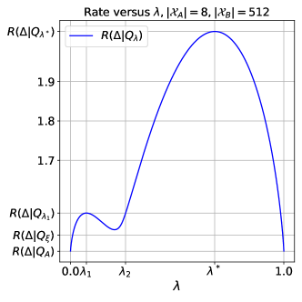
Figure 2: rate-distortion function $R(\Delta|Q_{\lambda})$ of Ahlswede’s counterexample with $|\mathcal{X}_{A}|=8$ as a function of $\lambda$. The unit of rate $R$ is the bit in all graphs in this section.

Next, let us draw the graph of the error exponent using the rate-distortion function in Fig. 2. We give the following theorem to evaluate the error exponent for Ahlswede’s counterexample.

Theorem 3

Assume the distortion measure $d(x,y)$ is given by (33) and let $P=Q_{\xi}$ for a fixed $\xi\in[0,1]$. Then, we have

$$E_{\rm M}(R|\Delta,Q_{\xi})=\min_{\genfrac{}{}{0.0pt}{}{\lambda\in[0,1]:}{R(\Delta|Q_{\lambda})\geq R}}D_{2}(\lambda\|\xi)$$ (40)

where $D_{2}(p\|q)=p\log\frac{p}{q}+(1-p)\log\frac{1-p}{1-q}$ is a binary divergence.

Before giving the proof, we state the following lemma due to Ahlswede [2].

Lemma 7

For any $P\in\mathcal{P(X)}$ with $\mathcal{X}=\mathcal{X}_{A}\cup\mathcal{X}_{B}$ where $\mathcal{X}_{A}$ and $\mathcal{X_{B}}$ are disjoint, define $\lambda=\sum_{x\in\mathcal{X}_{A}}P(x)$. We have

$$R(\Delta|\lambda Q_{A}+(1-\lambda)Q_{B})\geq R(\Delta|P).$$ (41)

See [2] for the proof.

Proof of Theorem 3: Let $q_{X}^{*}\in\mathcal{P(X)}$ be an optimal distribution that attains $E_{\rm M}(R|\Delta,Q_{\xi})=\min_{q_{X}:R(\Delta|q_{X})\geq R}D(q_{X}\|Q_{\xi}).$ Put $\lambda^{*}=\sum_{x\in\mathcal{X}_{A}}q_{X}^{*}(x)$. We will show that $q_{X}^{*}$ is expressed by $\lambda^{*}Q_{A}+(1-\lambda^{*})Q_{B}$.

Let $q_{A}^{*}(x)=q_{X}^{*}(x)/\lambda^{*}$ for $x\in\mathcal{X}_{A}$ and $q_{B}(x)=q_{X}^{*}(x)/(1-\lambda^{*})$ for $x\in\mathcal{X}_{B}$. Then, we have

$$D(q_{X}^{*}\|Q_{\xi})$$

$$=\sum_{x\in\mathcal{X}}q_{X}^{*}(x)\log\frac{q_{X}^{*}(x)}{Q_{\xi}(x)}$$

$$=\sum_{x\in\mathcal{X}_{A}}\lambda q_{A}^{*}(x)\log\frac{\lambda^{*}q_{A}^{*}(x)}{\frac{\xi}{|\mathcal{X}_{A}|}}$$

$$\quad+\sum_{x\in\mathcal{X}_{B}}(1-\lambda)q_{B}^{*}(x)\log\frac{(1-\lambda^{*})q_{B}^{*}(x)}{\frac{1-\xi}{|\mathcal{X}_{B}|}}$$

$$=\lambda^{*}\left\{\log\frac{\lambda^{*}|\mathcal{X}_{A}|}{\xi}+\sum_{x\in\mathcal{X}_{A}}q_{A}^{*}(x)\log q_{A}^{*}(x)\right\}$$

$$\quad+(1-\lambda^{*})\left\{\log\frac{(1-\lambda^{*})|\mathcal{X}_{B}|}{1-\xi}+\sum_{x\in\mathcal{X}_{B}}q_{B}^{*}(x)\log q_{B}^{*}(x)\right\}$$

$$\stackrel{{\scriptstyle(a)}}{{\geq}}\lambda^{*}\left\{\log\frac{\lambda^{*}|\mathcal{X}_{A}|}{\xi}-\log|\mathcal{X}_{A}|\right\}$$

$$\quad+(1-\lambda^{*})\left\{\log\frac{(1-\lambda^{*})|\mathcal{X}_{B}|}{1-\xi}-\log|\mathcal{X}_{B}|\right\}$$

$$=D_{2}(\lambda^{*}\|\xi)=D(\lambda^{*}Q_{A}+(1-\lambda^{*})Q_{B}\|Q_{\xi}),$$ (42)

Equality in (a) holds if and only if $q_{A}^{*}(x)=1/|\mathcal{X}_{A}|$ and $q_{B}^{*}(x)=1/|\mathcal{X}_{B}|$. From Lemma 7, we have $R(\Delta|\lambda^{*}Q_{A}+(1-\lambda^{*})Q_{B})\geq R(\Delta|q_{X}^{*})$ ($\geq R$). Therefore $\lambda^{*}Q_{A}+(1-\lambda^{*})Q_{B}$ is included in the feasible region $\{q_{X}:R(\Delta|q_{X})\geq R\}$. Since we assumed $q_{X}^{*}$ is optimal, we must have $q_{X}^{*}=\lambda^{*}Q_{A}+(1-\lambda^{*})Q_{B}$. This completes the proof. ∎

Theorem 3 ensures that the optimal error exponent can be computed as follows:

[Computation method of the error exponent for Ahlswede’s counterexample]

Let $N$ be a large positive integer and let $\lambda_{i}=i/N$ for $i=0,1,\ldots,N$. Compute $R_{i}=R(\Delta|Q_{\lambda_{i}})$ and $D_{i}=D_{2}(\lambda_{i}\|\xi)$. Then, arrange $(R_{i},D_{i})$ in ascending order of $R_{i}$. Put $E_{i}=\min_{j\geq i}D_{j}$. Then, by plotting $(R_{i},E_{i})$ for $i=0,1,\ldots,N$, we obtain the graph of $E=E_{\rm M}(R|\Delta,Q_{\xi})$ for $R(\Delta|Q_{\xi})\leq R\leq R_{\max}$. We can add a straight line segment $E=0$ for $0\leq R\leq R(\Delta|Q_{\xi})$.

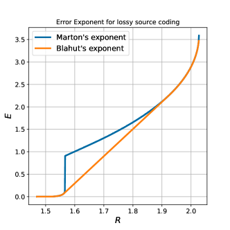
Figure 3: Marton’s and Blahut’s error exponents are illustrated as functions of $R$ for Ahlswede’s counterexample of Fig. 2, where $\Delta=0.254$ and $P=Q_{0.01}$.

Fig. 3 shows the error exponent for Ahlswede’s counterexample of Fig. 2. The probability distribution of the source is chosen as $P=Q_{\xi}$ with $\xi=0.01$. We observe that $E_{\rm M}(R|\Delta,P)=0$ for $R\leq R(\Delta|Q_{0.01})=1.510$ and $E_{\rm M}(R|\Delta,P)$ gradually increases for $1.510\leq R\leq R(\Delta|Q_{\lambda_{1}})=1.566$. At $R=1.566$, the curve jumps from $E=D(Q_{\lambda_{1}}\|Q_{\xi})=0.126$ to $E=D(Q_{\lambda_{2}}\|Q_{\xi})=0.904$, where $\lambda_{2}=0.258$ satisfies $R(\Delta|Q_{\lambda_{1}})=R(\Delta|Q_{\lambda_{2}})$. For $R(\Delta|Q_{\lambda_{1}})<R\leq R(\Delta|Q_{\lambda^{*}})$, the graph is expressed by $(R,E)=(R(\Delta|Q_{\lambda}),D(Q_{\lambda}\|Q_{\xi}))$ with $\lambda\in(\lambda_{2},\lambda^{*})$.

In Fig. 3, Blahut’s parametric expression (4) of error exponent is also plotted, where optimal distribution $p_{Y}^{*}$ for (4) is computed by Algorithm 2. This figure clearly shows that there is a gap between these two exponents.

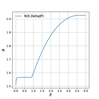
Figure 4: $R_{\rm M}(E|\Delta,P)$ for Ahlswede’s counterexample of Fig. 2.

Using the proposed method, we compute $R_{\rm M}(E|\Delta,P)$ for the same parameters for Fig. 3. The graph is shown in Fig. 4. It is confirmed that $R_{\rm M}(E|\Delta,P)$ is correctly computed. The inverse function is continuous in $E$ and if the inverse function takes a constant value $R_{0}$ for some finite interval $[E_{1},E_{2}]$, it means the error exponent jumps from $E_{1}$ to $E_{2}$ at $R=R_{0}$. Note that while Marton’s exponent in Fig 3 was computed based on Theorem 3, which holds only for Ahlswede’s counterexamples, the proposed method is applicable to any $P$, $d$, and $\Delta$ satisfying (8) and (9).

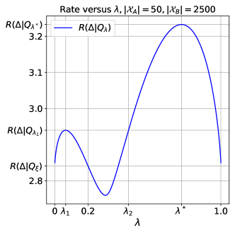
Figure 5: The rate-distortion function for the second example

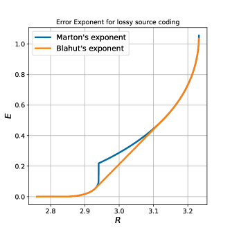
Figure 6: Error exponents for the second example

Here is another example to show the discontinuity of the optimal error exponent more clearly. Let $|\mathcal{X}_{A}|=50$ and $|\mathcal{X}_{B}|=|\mathcal{X}_{A}|^{2}$ and use the distortion measure (33) and determine the parameters $a=0.501$ and $\Delta=0.333$ to satisfy (38) and (39). The second example of Marton’s exponent is shown in Fig. 5. The global maximum is found at $\lambda^{*}=0.762$ and a local maximum at $\lambda=\lambda_{1}=0.065$. Then, the rate-distortion function of this case was computed by the Arimoto-Blahut algorithm. Marton’s and Blahut’s exponents are shown in Fig. 6, where $P=Q_{\xi}$ with $\xi=0.2$. We observe that Marton’s exponent jumps from $D(Q_{\lambda_{1}}\|Q_{0.2})=0.103$ to $D(Q_{\lambda_{2}}\|Q_{0.2})=0.220$ at $R=R(\Delta|Q_{\lambda_{1}})=R(\Delta|Q_{\lambda_{2}})=2.940$. In Fig. 7, $R_{\rm M}(E|\Delta,P)$ computed by the proposed method is drawn. We confirm that the graph is correctly computed.

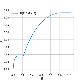
Figure 7: $R_{\rm M}(E|\Delta,P)$ for the second example

In Remark 1, it was stated that $\max_{p_{Y}}E_{0,s}^{(\rho,\nu)}(p_{Y}|P)$ is not necessarily concave in $\nu$. Here, we give an example to demonstrate that nonlinear optimization over $\nu$ is required to evaluate the Blahut’s exponent. Ahlswede’s counterexample with $|\mathcal{X}_{A}|=8$ and $|\mathcal{X}_{B}|=512$ is used and we put $\rho=2.25$. The graph in Fig. 8 shows $\max_{p_{Y}}E_{0,s}^{(\rho,\nu)}(p_{Y}|Q_{\lambda})-\rho\nu\Delta$ against $\nu$, where optimal $p_{Y}$ is computed by Algorithm 2. This figure clearly shows that there are two local maxima.

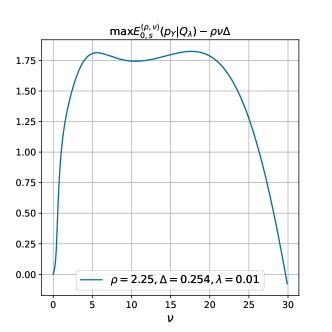
Figure 8: $\max_{p_{Y}}E_{0,s}^{(\rho,\nu)}(p_{Y}|Q_{\lambda})-\rho\nu\Delta$ as a function of $\nu$

V Proofs

This section gives the proofs of Property 2d) and Lemmas 1, 2, 5 and 6.

V-A Proof of Property 2d).

The continuity property of $R_{\rm M}(E|\Delta,P)$ is stated in Lemma 2 of [14]. However, the proof is not clear. In this section, we give a detailed proof of the continuity of $R_{\rm M}(E|\Delta,P)$.

We prove the continuity of $\widetilde{R}_{\rm M}(E|\Delta,P)$, which directly implies the continuity of $R_{\rm M}(E|\Delta,P)$. Before stating the proof, we give the following four lemmas necessary for the proof. The first and the second lemmas are the $L_{1}$ bounds on $R(\Delta|q)$ and $D(q||P)$ as functions of $q\in\mathcal{P(X)}$. The third and fourth lemmas are necessary to construct a delta-epsilon proof for Property 2d).

Lemma 8 (Palaiyanur and Sahai[15])

Suppose that the condition (8) is satisfied. Let $\tilde{d}=\min_{(x,y):d(x,y)>0}d(x,y)$. Then for any $p,q\in\mathcal{P(X)}$ such that $\lVert p-q\rVert_{1}\leq\tilde{d}/(4d_{\rm max})$ and $\Delta\geq 0$, we have

$$|R(\Delta|p)-R(\Delta|q)|\leq-\frac{7d_{\rm max}}{\tilde{d}}\lVert p-q\rVert_{1}\log\frac{\lVert p-q\rVert_{1}}{\lvert\mathcal{X}\rvert\lvert\mathcal{Y}\rvert}.$$ (43)

See [15] for the proof.

Next, we prove the following lemmas.

Lemma 9

Fix a $P\in\mathcal{P(X)}$. For any $p,q\in\mathcal{P(X)}$ such that $p(x)=q(x)=0$ if $P(x)=0$. If $\lVert p-q\rVert_{1}\leq\frac{1}{2}$, we have

$$\lvert D(p\|P)-D(q\|P)\rvert \leq-\lVert p-q\rVert_{1}\log\frac{\lVert p-q\rVert_{1}}{\lvert\mathcal{X}\rvert}$$

$$\quad-\lVert p-q\rVert_{1}\log\min_{\genfrac{}{}{0.0pt}{}{x\in\mathcal{X}:}{P(x)>0}}P(x)$$ (44)

Proof: Since $D(p\|P)=-H(p)-{\rm E}_{p}[\log P(X)]$ holds, $\lvert D(p\|P)-D(q\|P)\rvert$ is upper bounded by $|H(p)-H(q)|+|{\rm E}_{p}[\log P(X)]-{\rm E}_{q}[\log P(X)]|$. We use the $L_{1}$ bound on entropy [1, Theorem 17.3.3], i.e., $|H(p)-H(q)|\leq-\lVert p-q\rVert_{1}\log\frac{\lVert p-q\rVert_{1}}{|\mathcal{X}|}$ if $\lVert p-q\rVert_{1}\leq 1/2$. Let $r(x)=|p(x)-q(x)|$. The second term is upper bounded as follows.

$$|{\rm E}_{p}[\log P(X)]-{\rm E}_{q}[\log P(X)]|$$

$$=\left|\sum_{x\in\mathcal{X}}(p(x)-q(x))\log P(x)\right|$$

$$\leq-\sum_{x\in\mathcal{X}}r(x)\log P(x)$$

$$=-\lVert p-q\rVert_{1}\sum_{x\in\mathcal{X}}\frac{r(x)}{\lVert p-q\rVert_{1}}\log P(x)$$

$$\leq-\lVert p-q\rVert_{1}\log\min_{\genfrac{}{}{0.0pt}{}{x\in\mathcal{X}:}{P(x)>0}}P(x).$$ (45)

The proof is completed by adding the upper bounds of the two terms. ∎

Lemma 10

For any $\epsilon>0$ and any $p_{X}\in\mathcal{P(X)}$, there exists a $\xi=\xi(\epsilon)$ such that for any $q_{X}\in\mathcal{P(X)}$ with $\lVert p_{X}-q_{X}\rVert\leq\xi(\epsilon)$ satisfies $\lvert R(\Delta|p_{X})-R(\Delta|q_{X})\rvert\leq\epsilon$. This implies that for any $\epsilon>0$ and $p_{X}\in\mathcal{P(X)}$, there exists a $\xi=\xi(\epsilon)>0$ such that the following two inequalities hold.

$$\max_{\genfrac{}{}{0.0pt}{}{q_{X}\in\mathcal{P(X)}:}{\lVert p_{X}-q_{X}\rVert_{2}\leq\xi}}R(\Delta|q_{X})\leq R(\Delta|p_{X})+\epsilon,$$ (46)

$$\min_{\genfrac{}{}{0.0pt}{}{q_{X}\in\mathcal{P(X)}:}{\lVert p_{X}-q_{X}\rVert_{2}\leq\xi}}R(\Delta|q_{X})\geq R(\Delta|p_{X})-\epsilon.$$ (47)

Proof: By Lemma 8, there exists a $\xi^{\prime}(\epsilon)>0$ such that for any $p_{X},q_{X}\in\mathcal{P(X)}$ satisfying $\lVert p_{X}-q_{X}\rVert_{1}\leq\xi^{\prime}(\epsilon)$,

$$|R(\Delta|p_{X})-R(\Delta|q_{X})|\leq\epsilon$$ (48)

holds. Fix this $\xi^{\prime}(\epsilon)$ and put $\xi(\epsilon)=\xi^{\prime}(\epsilon)/\sqrt{|\mathcal{X}|}$. Then, due to the Cauchy-Schwartz inequality, for any $p_{X},q_{X}\in\mathcal{P(X)}$ satisfying $\lVert p_{X}-q_{X}\rVert_{2}\leq\xi(\epsilon)$, we have $\lVert p_{X}-q_{X}\rVert_{1}\leq\sqrt{|\mathcal{X}|}\,\lVert p_{X}-q_{X}\rVert_{2}\leq\xi^{\prime}(\epsilon)$. Hence, from (48), we have

$$R(\Delta|p_{X})-\epsilon\leq R(\Delta|q_{X})\leq R(\Delta|p_{X})+\epsilon.$$ (49)

for any $p_{X}$, $q_{X}\in\mathcal{P(X)}$ with $\lVert p_{X}-q_{X}\rVert_{2}\leq\delta(\epsilon)$. Taking the minimum and the maximum values of $R(\Delta|q_{X})$ w.r.t. $q_{X}$, we obtain (46) and (47). This completes the proof. ∎

Lemma 11

For any $E\in[0,E^{*}]$ and any $\xi>0$, there exists a $\delta(E,\xi)>0$ such that for any $p_{X}\in\mathcal{P(X)}$ satisfying

$$E-\delta(E,\xi)\leq D(p_{X}\|P)\leq E+\delta(E,\xi),$$ (50)

there exists a $q_{X}\in\mathcal{P(X)}$ satisfying

$$D(q_{X}\|P) =E,$$ (51)

$$\lVert p_{X}-q_{X}\rVert_{2} \leq\xi.$$ (52)

Proof: Fix $E\in[0,E^{*}]$ and $\xi>0$ arbitrarily. Assume, for the sake of contradiction, that for any positive integer $n$, there exists a $p_{X}^{(n)}$ satisfying

$$|D(p_{X}^{(n)}\|P)-E|\leq\delta_{n}$$ (53)

with $\delta_{n}=1/n$ such that for any $q_{X}\in\mathcal{P(X)}$ satisfying $D(q_{X}\|P)=E$, we have

$$\lVert p_{X}^{(n)}-q_{X}\rVert_{2}>\xi.$$ (54)

Since the space $\mathcal{P(X)}$ is a closed bounded subset of $\mathbb{R}^{|\mathcal{X}|}$, it follows from the Bolzano-Weierstrass theorem that the sequence $\{p_{X}^{(n)}\}$ has a subsequence converging to an element in $\mathcal{P(X)}$. That is, there exists $q_{X}^{*}\in\mathcal{P(X)}$ and $k_{n}$, $n=1,2,\ldots$ such that

$$\lVert p_{X}^{(k_{n})}-p_{X}^{*}\rVert_{2}\to 0,n\to\infty$$ (55)

For any $|\mathcal{X}|$-dimensional vector $r$, the Cauchy-Schwarz inequality gives $\lVert r\rVert_{1}\leq\sqrt{\lvert\mathcal{X}\rvert}\,\lVert r\rVert_{2}$. Thus, (55) implies

$$\|p_{X}^{(k_{n})}-p_{X}^{*}\|_{1}\to 0,\quad n\to\infty.$$ (56)

Note that $p_{X}$ for which $D(p_{X}\|P)$ is finite satisfies $p_{X}(x)=0$ if $P(x)=0$. Then, it follows from Lemma 9 and (56) that

$$|D(p_{X}^{(k_{n})}\|P)-D(p_{X}^{*}\|P)|\to 0,\quad n\to\infty.$$ (57)

From (53) and the continuity of $D(p_{X}\|P)$ in $p_{X}\in\mathcal{P(X)}$, we have

$$\lim_{n\to\infty}D(p_{X}^{(k_{n})}\|P)=D(p_{X}^{*}\|P)=E.$$ (58)

Then, by choosing $q_{X}=p_{X}^{*}$, we have $D(q_{X}\|P)=E$ and

$$\lVert p_{X}^{(n)}-q_{X}\rVert_{2}=\lVert p_{X}^{(n)}-p_{X}^{*}\rVert_{2}\to 0,\quad n\to\infty.$$ (59)

This is a contradiction. Hence the first assumption was wrong and the statement of the lemma holds. This completes the proof. ∎

Proof of Property 2d): We first prove the continuity of $\widetilde{R}(E|\Delta,P)$ in $E$. By Lemma 10, for any $\epsilon>0$, there exists a $\xi=\xi(\epsilon)$ such that any $p_{X}\in\mathcal{P(X)}$ satisfies (46) and (47). Fix this $\xi(\epsilon)$. For this choice of $\xi(\epsilon)$ and any $E\in[0,E_{*}]$, from Lemma 11 there exists a $\delta=\delta(E,\xi(\epsilon))>0$ such that for any $p_{X}\in\mathcal{P(X)}$ satisfying $|D(p_{X}\|P)-E|\leq\delta$ there exists a $q_{X}\in\mathcal{P(X)}$ satisfying $D(q_{X}\|P)=E$ and $\lVert p_{X}-q_{X}\rVert_{2}\leq\xi(\epsilon)$. Then, for any for any $E^{\prime}\in[E-\delta,E+\delta]$, the following chain of inequalities holds.

$$\widetilde{R}(E^{\prime}|\Delta,P)$$

$$\max_{\genfrac{}{}{0.0pt}{}{p_{X}\in\mathcal{P(X)}}{D(p_{X}\|P)=E^{\prime}}}R(\Delta|p_{X})$$

$$\stackrel{{\scriptstyle\rm(a)}}{{\leq}}\max_{\genfrac{}{}{0.0pt}{}{p_{X}\in\mathcal{P(X)}}{D(p_{X}\|P)=E^{\prime}}}\min_{\genfrac{}{}{0.0pt}{}{q_{X}\in\mathcal{P(X)}}{\lVert p_{X}-q_{X}\rVert_{2}\leq\xi(\epsilon)}}R(\Delta|q_{X})+\epsilon$$

$$\stackrel{{\scriptstyle\rm(b)}}{{\leq}}\max_{\begin{subarray}{c}p_{X}\in\mathcal{P(X)}\\ D(p_{X}\|P)=E^{\prime}\end{subarray}}\min_{\begin{subarray}{c}q_{X}\in\mathcal{P(X)}:\\ \lVert p_{X}-q_{X}\rVert_{2}\leq\xi(\epsilon)\\ D(q_{X}\|P)=E\end{subarray}}R(\Delta|q_{X})+\epsilon$$

$$\stackrel{{\scriptstyle\rm(c)}}{{\leq}}\max_{\begin{subarray}{c}p_{X}\in\mathcal{P(X)}\\ D(p_{X}\|P)=E^{\prime}\end{subarray}}\min_{\begin{subarray}{c}q_{X}\in\mathcal{P(X)}:\\ \lVert p_{X}-q_{X}\rVert_{2}\leq\xi(\epsilon)\\ D(q_{X}\|P)=E\end{subarray}}\widetilde{R}(E|\Delta,P)+\epsilon$$

$$\stackrel{{\scriptstyle\rm(d)}}{{=}}\widetilde{R}(E|\Delta,P)+\epsilon$$ (60)

Step (a) follows from (47). Step (b) holds because additional constraint on the minimization increases the minimum value. Step (c) follows from that the maximum value of $R(\Delta|q_{X})$ under the condition $D(q_{X}\|P)=E$ and a fixed $\Delta$ is given by $\tilde{R}(E|\Delta,P)$. Step (d) holds because for any $p_{X}$ satisfying $D(p_{X}||P)=E^{\prime}$, there exists $q_{X}\in\mathcal{P(X)}$ satisfying $D(p_{X}\|P)=E^{\prime}$, $D(q_{X}\|P)=E$, and $\lVert p_{X}-q_{X}\rVert_{2}\leq\xi(\epsilon)$ due to Lemma 11.

On the other hand, for any $E^{\prime}\in[E-\delta,E+\delta]$, we have the following chain of inequalities.

$$\widetilde{R}(E^{\prime}|\Delta,P)$$

$$\max_{\genfrac{}{}{0.0pt}{}{p_{X}\in\mathcal{P(X)}}{D(p_{X}\|P)=E^{\prime}}}R(\Delta|p_{X})$$

$$\stackrel{{\scriptstyle\rm(a)}}{{\geq}}\max_{\genfrac{}{}{0.0pt}{}{p_{X}\in\mathcal{P(X)}}{D(p_{X}\|P)=E^{\prime}}}\max_{\genfrac{}{}{0.0pt}{}{q_{X}\in\mathcal{P(X)}}{\lVert p_{X}-q_{X}\rVert\leq\xi(\epsilon)}}R(\Delta|q_{X})-\epsilon$$

$$\stackrel{{\scriptstyle\rm(b)}}{{\geq}}\max_{\begin{subarray}{c}p_{X}\in\mathcal{P(X)}\\ D(p_{X}\|P)=E^{\prime}\end{subarray}}\max_{\begin{subarray}{c}q_{X}\in\mathcal{P(X)}:\\ \lVert p_{X}-q_{X}\rVert\leq\xi(\epsilon)\\ D(q_{X}\|P)=E\end{subarray}}R(\Delta|q_{X})-\epsilon$$

$$\stackrel{{\scriptstyle\rm(c)}}{{=}}\max_{\begin{subarray}{c}q_{X}\in\mathcal{P(X)}:\\ D(q_{X}\|P)=E\end{subarray}}R(\Delta|q_{X})-\epsilon$$

$$=\widetilde{R}(E|\Delta,P)-\epsilon$$ (61)

Step (a) follows from (46). Step (b) holds because additional constraint on the maximization decreases the maximum value. Step (c) follows from that, by Lemma 11, for any $p_{X}$ satisfying $D(p_{X}\|P)=E^{\prime}$, there exists $q_{X}$ such that $D(q_{X}\|P)=E$ and $\lVert p_{X}-q_{X}\rVert\leq\xi(\epsilon)$ hold and that the objective function $R(\Delta|q_{X})$ is independent of $p_{X}$. Combining (60) and (61), we have

$$\lvert\widetilde{R}(E|\Delta,P)-\widetilde{R}(E^{\prime}|\Delta,P)\rvert<\epsilon.$$ (62)

This proves the continuity of $\widetilde{R}(E|\Delta,P)$. The continuity of $R(E|\Delta,P)$ follows directly from (11), which completes the proof. ∎

V-B Proofs of Lemmas

In this subsection, we give the proofs of Lemmas 1, 2, 5, and 6.

Proof of Lemma 1: Let $\rho$ be any non-negative number and $q_{X}^{*}$ be an optimal distribution that achieves $E_{\rm M}(R|\Delta,P)=\min_{q_{X}:R(\Delta|q_{X})\geq R}D(q_{X}\|P)$. Then, we have

$$E_{\rm M}(R|\Delta,P)=D(q_{X}^{*}\|P)$$

$$\stackrel{{\scriptstyle\rm(a)}}{{\geq}}\{D(q_{X}^{*}\|P)-\rho[R(\Delta|q_{X}^{*})-R]\}$$

$$\geq\min_{q_{X}:R(\Delta|q_{X})\geq R}\{D(q_{X}\|P)-\rho[R(\Delta|q_{X})-R]\}$$

$$\geq\min_{q_{X}\in\mathcal{P(Y)}}\{D(q_{X}\|P)-\rho[R(\Delta|q_{X})-R]\}$$

$$\stackrel{{\scriptstyle\rm(b)}}{{=}}\rho R+\min_{q_{X}\in\mathcal{P(Y)}}\Big{\{}D(q_{X}\|P)-\rho\sup_{\nu\geq 0}\Big{[}-\nu\Delta$$

$$\quad-\max_{p_{Y}}\sum_{x}q_{X}(x)\log p_{Y}(y){\rm e}^{-\nu d(x,y)}\Big{]}\Big{\}}$$

$$=\rho R+\inf_{\nu\geq 0}\min_{q_{X}}\max_{p_{Y}}\Big{[}\rho\nu\Delta+D(q_{X}\|P)$$

$$\hskip 56.9055pt+\rho\sum_{x}q_{X}(x)\log\sum_{y}p_{Y}(y){\rm e}^{-\nu d(x,y)}\Big{]}$$

$$\stackrel{{\scriptstyle\rm(c)}}{{=}}\rho R+\inf_{\nu\geq 0}\max_{p_{Y}}\min_{q_{X}}\Big{[}\rho\nu\Delta+D(q_{X}\|P)$$

$$\hskip 56.9055pt+\rho\sum_{x}q_{X}(x)\log\sum_{y}p_{Y}(y){\rm e}^{-\nu d(x,y)}\Big{]}$$

$$\stackrel{{\scriptstyle\rm(d)}}{{=}}\rho R+\inf_{\nu\geq 0}\bigg{[}\rho\nu\Delta$$

$$\quad+\max_{p_{Y}}-\log\sum_{x}P(x)\Big{\{}\sum_{y}p_{Y}(y){\rm e}^{-\nu d(x,y)}\Big{\}}^{-\rho}\bigg{]}.$$ (63)

Step (a) holds because $q^{*}_{X}$ satisfies $R(\Delta|q_{X})\geq R$. In Step (b), Eq.(12) is substituted. Step (c) follows from the minimax theorem. It holds because $D(q_{X}\|P)$ is a convex function of $q_{X}$ and $\sum_{x}q_{X}(x)\log p_{Y}(y){\rm e}^{-\nu d(x,y)}$ is linear in $q_{X}$ and concave in $p_{Y}$. Step (d) holds because we have

$$D(q_{X}\|P)+\rho\sum_{x}q_{X}(x)\log\sum_{y}p_{Y}(y){\rm e}^{-\nu d(x,y)}$$

$$=\sum_{x}q_{X}(x)\log\frac{q_{X}(x)}{P(x)\{\sum_{y}p_{Y}(y){\rm e}^{-\nu d(x,y)}\}^{-\rho}}$$

$$=\sum_{x}q_{X}(x)\log\frac{q_{X}(x)}{\frac{1}{K}P(x)\{\sum_{y}p_{Y}(y){\rm e}^{-\nu d(x,y)}\}^{-\rho}}-\log K$$

$$\stackrel{{\scriptstyle\rm(e)}}{{\geq}}-\log K,$$ (64)

where $K=\sum_{x\in\mathcal{X}}P(x)\{\sum_{y}p_{Y}(y){\rm e}^{-\nu d(x,y)}\}^{-\rho}$. In Step (e), equality holds when $q_{X}(x)=\frac{1}{K}P(x)\{\sum_{y}p_{Y}(y)\cdot{\rm e}^{-\nu d(x,y)}\}^{-\rho}$. Because Eq. (63) holds any $\rho\geq 0$, we have

$$E_{\rm M}(R|\Delta,P)$$

$$\geq\sup_{\rho\geq 0}\bigg{\{}\rho R+\inf_{\nu\geq 0}\bigg{[}\rho\nu\Delta$$

$$\quad+\max_{p_{Y}}-\log\sum_{x}P(x)\Big{\{}\sum_{y}p_{Y}(y){\rm e}^{-\nu d(x,y)}\Big{\}}^{-\rho}\bigg{]}\bigg{\}}$$

$$=E_{\rm B}(R|\Delta,P_{X}).$$ (65)

This completes the proof. ∎

Proof of Lemma 2: Let $\check{q}_{X}$ be a distribution that attains $R_{\rm M}(E|\Delta,P)$ and let $\check{E}=D(\check{q}_{X}\|P)$. Then we have

$$\max_{E^{\prime}\leq E}\widetilde{R}(E^{\prime}|\Delta,P)$$

$$\stackrel{{\scriptstyle\rm(a)}}{{\geq}}\widetilde{R}(\check{E}|\Delta,P)$$

$$=\max_{\genfrac{}{}{0.0pt}{}{q_{X}\in\mathcal{P(X)}:}{D(q_{X}\|P)=\check{E}}}R(\Delta|q_{X})$$

$$\stackrel{{\scriptstyle\rm(b)}}{{\geq}}R(\Delta|\check{q}_{X})=R_{\rm M}(E|\Delta,P).$$ (66)

Step (a) follows from that $\check{E}$ is smaller than or equal to $E$ because of the definition of $\check{E}$. Step (b) holds because $\check{q}_{X}$ satisfies $D(\check{q}_{X}\|P)=\check{E}$.

On the other hand, let $\widehat{E}^{\prime}$ and $\hat{q}_{X}$ be an $E^{\prime}$ and $q_{X}$ that attains $\max_{E^{\prime}\leq E}\max_{\genfrac{}{}{0.0pt}{}{q_{X}\in\mathcal{P(X)}:}{D(q_{X}\|P)=E^{\prime}}}R(\Delta|q_{X})$. Then we have

$$R_{\rm M}(E|\Delta,P)$$

$$=\max_{\genfrac{}{}{0.0pt}{}{q_{X}\in\mathcal{P(X)}:}{D(q_{X}\|P)\leq E}}R(\Delta|q_{X})$$

$$\stackrel{{\scriptstyle\rm(a)}}{{\geq}}\max_{\genfrac{}{}{0.0pt}{}{q_{X}\in\mathcal{P(X)}:}{D(q_{X}\|P)\leq\hat{E}^{\prime}}}R(\Delta|q_{X})$$

$$\stackrel{{\scriptstyle\rm(b)}}{{\geq}}R(\Delta|\hat{q}_{X})=\max_{E^{\prime}\leq E}\widetilde{R}(E^{\prime}|\Delta,P).$$ (67)

Step (a) follows from that $\hat{E}^{\prime}\leq E$ because of the definition. Step (b) follows from that $\hat{q}_{X}$ satisfies $D(\hat{q}_{X}\|P)=\widehat{E}^{\prime}$.

From (66) and (67), we have (11), completing the proof. ∎

Proof of Lemma 5: If $\mu=0$, we have

$$G^{(0,\nu)}(p_{Y}|P) =\max_{q_{X}}-\sum_{x}q_{X}(x)\log\sum_{y}p_{Y}(y){\rm e}^{-\nu d(x,y)}$$

$$=-\log\min_{x}\sum_{y}p_{Y}(y){\rm e}^{-\nu d(x,y)}.$$ (68)

The maximum is attained by $q_{X}(x)=1$ for $x=\arg\min_{x}\sum_{y}p_{Y}(y){\rm e}^{-\nu d(x,y)}$. If $\mu>0$, we have

$$G^{(\mu,\nu)}(p_{Y}|P)$$

$$=-\mu\min_{q_{X}}\left[\sum_{x}q_{X}(x)\log\frac{q_{X}(x)}{P(x)\left[\sum_{y}p_{Y}(y)\mathrm{e}^{-\nu d(x,y)}\right]^{-1/\mu}}\right]$$

$$=-\mu\min_{q_{X}}D(q_{X}\|q_{X}^{*})+\mu\log K$$

$$=\mu\log K,$$

where $q_{X}^{*}(x)=\frac{1}{K}P(x)\left[\sum_{y}p_{Y}(y)\mathrm{e}^{-\nu d(x,y)}\right]^{-1/\mu}$ and $K=\sum_{x}P(x)\left\{\sum_{y}q_{Y}(y)\mathrm{e}^{-\nu d(x,y)}\right\}^{-1/\mu}$. This completes the proof. ∎

Before describing the proof of Lemma 6, we show that the function $G^{(\nu)}(E,p_{Y}|P)$ satisfies the following property:

Property 3

For fixed $\nu\geq 0$, $p_{Y}$, and $P$, $G^{(\nu)}(E,p_{Y}|P)$ is a monotone non-decreasing and concave function of $E\geq 0$.

Proof of Property 3: Monotonicity is obvious from the definition. Let us prove the concavity. Choose $E_{0},E_{1}\geq 0$ arbitrarily. Set $E_{\alpha}=\alpha E_{1}+(1-\alpha)E_{0}$ for $\alpha\in[0,1]$. Let the optimal distribution that attains $G^{(\nu)}(p_{Y},E_{0}|P)$ and $G^{(\nu)}(p_{Y},E_{1}|P)$ be $q_{X}^{0}$ and $q_{X}^{1}$. Then we have $D(q_{X}^{i}\|P)\leq E_{i}$ for $i=0,1$. By the convexity of the KL divergence, we have $D(\alpha q_{X}^{1}+(1-\alpha)q_{X}^{0}\|P)\leq\alpha D(q_{X}^{1}\|P)+(1-\alpha)D(q_{X}^{0}\|P)\leq\alpha E_{0}+(1-\alpha)E_{1}=E_{\alpha}.$ Therefore we have

$$G^{(\mu)}(p_{Y}|E_{\alpha},P)$$

$$=\sup_{\genfrac{}{}{0.0pt}{}{q_{X}\in\mathcal{P(X)}:}{D(q_{X}\|P)\leq E_{\alpha}}}\Big{\{}-\sum_{x}q_{X}(x)\log\sum_{y}p_{Y}(y){\rm e}^{-\nu d(x,y)}\Big{\}}$$

$$\geq\left.-\sum_{x}q_{X}(x)\log\sum_{y}p_{Y}(y){\rm e}^{-\nu d(x,y)}\right|_{q_{X}=\alpha q_{X}^{1}+(1-\alpha)q_{X}^{0}}$$

$$=\alpha G^{(\nu)}(p_{Y},E_{1}|P)+(1-\alpha)G^{(\nu)}(p_{Y},E_{0}|P).$$ (69)

This completes the proof. ∎

Proof of Lemma 6: We prove that (i) for any $\mu\geq 0$ $G^{(\nu)}(E,p_{Y}|P)\leq G^{(\mu,\nu)}(p_{Y}|P)+\mu E$ holds and (ii) there exists a $\mu\geq 0$ such that $G^{(\nu)}(E,p_{Y}|P)\geq G^{(\mu,\nu)}(p_{Y}|P)+\mu E$ holds.

Part (i): For any $\mu\geq 0$, we have

$$G^{(\nu)}(p_{Y},E|P)$$

$$=\sup_{\genfrac{}{}{0.0pt}{}{q_{X}\in\mathcal{P(X)}:}{D(q_{X}\|P)\leq E}}\Big{\{}-\sum_{x}q_{X}(x)\log\sum_{y}p_{Y}(y){\rm e}^{-\nu d(x,y)}\Big{\}}$$

$$\stackrel{{\scriptstyle\rm(a)}}{{\leq}}\sup_{\genfrac{}{}{0.0pt}{}{q_{X}\in\mathcal{P(X)}:}{D(q_{X}\|P)\leq E}}\Big{\{}-\sum_{x}q_{X}(x)\log\sum_{y}p_{Y}(y){\rm e}^{-\nu d(x,y)}$$

$$\quad\quad+\mu(E-D(q_{X}\|P))\Big{\}}$$

$$\stackrel{{\scriptstyle\rm(b)}}{{\leq}}\sup_{q_{X}\in\mathcal{P(X)}:}\Big{\{}-\sum_{x}q_{X}(x)\log\sum_{y}p_{Y}(y){\rm e}^{-\nu d(x,y)}$$

$$\quad\quad+\mu(E-D(q_{X}\|P))\Big{\}}$$

$$=\mu E+G^{(\mu,\nu)}(p_{X}|P).$$ (70)

Step (a) holds because adding a positive term $\mu(E-D(q_{X}||P))$ to the objective function does not decrease the supremum. Step (b) holds because removing the restriction for the domain of the variable $q_{X}$ does not decrease the supremum. Thus Part (i) is proved.

Part (ii): From Property 3, for a fixed $E\geq 0$, there exist a $\mu\geq 0$ such that for any $E^{\prime}$ we have

$$G^{(\nu)}(p_{Y},E^{\prime}|P)\leq G^{(\nu)}(p_{Y},E|P)+\mu(E^{\prime}-E).$$ (71)

Fix this $\mu=\mu(E)$ and let $q_{X}^{\prime}$ be a probability distribution that attains the right-hand side of (18) for this choice of $\mu$. Put $E^{\prime}=D(q_{X}^{\prime}||P)$ for this $q_{X}^{\prime}$ and then we have

$$G^{(\nu)}(p_{Y},E|P)$$

$$\stackrel{{\scriptstyle\rm(a)}}{{\geq}}G^{(\nu)}(p_{Y},E^{\prime}|P)-\mu(D(q_{X}^{\prime}||P)-E)$$

$$\stackrel{{\scriptstyle\rm(b)}}{{\geq}}-\sum_{x}q_{X}^{\prime}(x)\log\sum_{y}p_{Y}(y){\rm e}^{-\nu d(x,y)}$$

$$\quad+\mu E-\mu D(q_{X}^{\prime}\|P)$$

$$\stackrel{{\scriptstyle\rm(c)}}{{=}}\mu E+G^{(\mu,\nu)}(p_{Y}|P).$$ (72)

Step (a) follows form (71) and the choice of $E^{\prime}$. Step (b) holds because $q_{X}^{\prime}$ satisfies $D(q_{X}^{\prime}||P)\leq E^{\prime}$ and therefore is a feasible variable for $G^{(\nu)}(p_{Y},E^{\prime}|P)$. Step (c) holds because of the choice of $q_{X}^{\prime}$. This proves Part (ii), which completes the proof. ∎

References

- [1] T. M. Cover and J. A. Thomas, Elements of Information Theory, 2nd ed. Wiley-Interscience, 2006.
- [2] R. Ahlswede, “External properties of rate-distortion functions,” IEEE Trans. Inform. Theory, vol. 36, no. 1, pp. 166–171, 1990.
- [3] D. R. Marton, “Error exponent for source coding with a fidelity criterion,” IEEE Trans. Inform. Theory, vol. 20, pp. 197–199, 1974.
- [4] R. Blahut, “Computation of channel capacity and rate distortion functions,” IEEE Trans. Inform. Theory, vol. 18, pp. 460–473, 1972.
- [5] S. Arimoto, “An algorithm for calculating the capacity of an arbitrary discrete memoryless channel,” IEEE Trans. Inform. Theory, vol. IT-18, pp. 14–20, 1972.
- [6] ——, “Computation of random coding exponent functions,” IEEE Trans. Inform. Theory, vol. IT-22, no. 6, pp. 665–671, 1976.
- [7] R. Blahut, “Hypothesis testing and information theory,” IEEE Trans. Inform. Theory, vol. 20, pp. 405 – 417, 1974.
- [8] E. Arıkan and N. Merhav, “Guessing subject to distortion,” IEEE Trans. Inform. Theory, vol. 44, no. 3, pp. 1041–1056, 1998.
- [9] E. Haroutunian and B. Mekoush, “Estimates of optimal rates of codes with given error probability exponent for certain sources,” in 6th Int. Symp. on Information Theory (in Russian), vol. 1, 1984, pp. 22–23.
- [10] A. N. Harutyunyan and E. A. Haroutunian, “On properties of rate-reliability-distortion functions,” IEEE Trans. Information Theory, vol. 50, no. 11, pp. 2768–2773, 2004.
- [11] I. Csiszár and J. Körner, Information theory, coding theorems for discrete memoryless systems. Academic Press, 1981.
- [12] V. Kostina and S. Verdú, “Fixed-length lossy compression in the finite blocklength regime,” IEEE Transactions on Information Theory, vol. 58, no. 6, pp. 3309–3338, 2012.
- [13] M. Sion, “On general minimax theorems,” Pacific J. Math, vol. 8, no. 1, pp. 171–176, 1958.
- [14] E. A. Haroutunian, A. N. Harutyunyan, and A. R. Ghazaryan, “On rate-reliability-distortion function for a robust descriptions system,” IEEE Trans. Information Theory, vol. 46, no. 7, pp. 2690–2697, 2000.
- [15] H. Palaiyanur and A. Sahai, “On the uniform continuity of the rate-distortion function,” in 2008 IEEE Int. Symp. Inform. Theory. IEEE, 2008, pp. 857–861.