MultiGPrompt for Multi-Task Pre-Training
and Prompting on Graphs

Abstract.

Graph Neural Networks (GNNs) have emerged as a mainstream technique for graph representation learning. However, their efficacy within an end-to-end supervised framework is significantly tied to the availability of task-specific labels. To mitigate labeling costs and enhance robustness in few-shot settings, pre-training on self-supervised tasks has emerged as a promising method, while prompting has been proposed to further narrow the objective gap between pretext and downstream tasks. Although there has been some initial exploration of prompt-based learning on graphs, they primarily leverage a single pretext task, resulting in a limited subset of general knowledge that could be learned from the pre-training data. Hence, in this paper, we propose MultiGPrompt, a novel multi-task pre-training and prompting framework to exploit multiple pretext tasks for more comprehensive pre-trained knowledge. First, in pre-training, we design a set of pretext tokens to synergize multiple pretext tasks. Second, we propose a dual-prompt mechanism consisting of composed and open prompts to leverage task-specific and global pre-training knowledge, to guide downstream tasks in few-shot settings. Finally, we conduct extensive experiments on six public datasets to evaluate and analyze MultiGPrompt.

1. Introduction

The Web has evolved into an universal data repository, linking an expansive array of entities to create vast and intricate graphs. Mining such widespread graph data has fueled a myriad of Web applications, ranging from Web mining (Xu et al., 2022; Agarwal et al., 2022) and social network analysis (Zhang et al., 2022; Zhou et al., 2023) to content recommendation (Qu et al., 2023; Zhu et al., 2023). Contemporary techniques for graph analysis predominantly rely on graph representation learning, particularly graph neural networks (GNNs) (Kipf and Welling, 2017; Veličković et al., 2018; Fang et al., 2023a, b; Yu et al., 2023a). Most GNNs operate on a message-passing framework, where each node updates its representation by iteratively receiving and aggregating messages from its neighbors (Wang et al., 2023a, 2022b; Anonymous, 2024b, a; Wang et al., 2023b; Li et al., 2023, 2024b), while more recent approaches have also explored transformer-based architectures (Yun et al., 2019; Hu et al., 2020a; Wu et al., 2024).

Pre-training. GNNs are conventionally trained in an end-to-end manner, which heavily depends on the availability of large-scale, task-specific labeled data. To reduce the dependency on labeled data, there has been a growing emphasis on pre-training GNNs (Hu et al., 2020b, c; Qiu et al., 2020; Lu et al., 2021; Yu et al., 2024a), following the success of pre-training in natural language and computer vision domains (Erhan et al., 2010; Dong et al., 2019; Bao et al., 2022). Pre-training GNNs involves optimizing self-supervised pretext tasks on graphs without task-specific labels. Such pretext tasks are designed to capture intrinsic graph properties, such as node and edge features (Hu et al., 2020c, b; You et al., 2020), node connectivity (Hamilton et al., 2017; Hu et al., 2020b; You et al., 2020; Lu et al., 2021), and local or global graph patterns (Veličković et al., 2018; You et al., 2020; Qiu et al., 2020; Hu et al., 2020c; Lu et al., 2021). Hence, pre-training yields a task-agnostic foundation that can be subsequently fine-tuned to a specific downstream task with a limited amount of labeled data. To further mitigate the inconsistency between pre-training and fine-tuning objectives (Liu et al., 2021b), prompt-based learning has been first proposed in language models (Brown et al., 2020). A prompt acts as an intermediary that reformulates the downstream task to align with pre-training, without the need to update the parameters of the pre-trained model. As a prompt entails much fewer parameters than the pre-trained model, it is especially amenable to few-shot settings where there are very limited task-specific labels.

Following the success of prompt-based learning, researchers have also begun to explore prompt-based or related parameter-efficient learning on graph data (Liu et al., 2023a; Sun et al., 2023, 2022; Tan et al., 2023; Fang et al., 2022; Li et al., 2024a; Yu et al., 2024b). However, most existing research in prompt-based graph learning only utilizes a single pretext task in pre-training. Not surprisingly, different pretext tasks capture different self-supervised signals from the graph. For example, link prediction tasks are more concerned with the connectivity or relationship between nodes (Sun et al., 2022), node/edge feature-based tasks focus more on the feature space (Tan et al., 2023), and subgraph-based tasks focus more on local or global information (Liu et al., 2023a; Yi et al., 2023). To cater to diverse downstream tasks, the pre-training step should aim to broadly extract knowledge from various aspects, such as node connectivity, node or edge features, and local or global graph patterns. Hence, it is ideal to incorporate multiple pretext tasks in pre-training in order to cover a comprehensive range of knowledge.

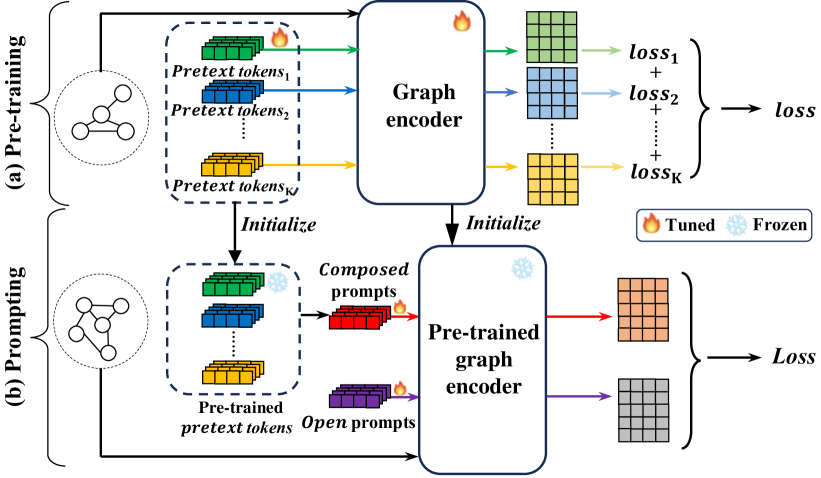
Figure 1. Illustration of MultiGPrompt. (a) Multi-task pre-training on graphs. (b) Prompting on downstream tasks.

Challenges. To address the limitation of a single pretext task, in this work we study multi-task pre-training for graphs and the effective transfer of multi-task knowledge to downstream few-shot tasks. The problem is non-trivial due to the following two challenges.

First, in the pre-training stage, how can we leverage diverse pretext tasks for graph models in a synergistic manner? A straightforward way is to sum the losses of multiple pretext tasks directly, which have been explored in language (Devlin et al., 2018; Su et al., 2021; Wu et al., 2021), vision (Mormont et al., 2020; Gong et al., 2021) and graph data (Hu et al., 2019, 2020b; Lu et al., 2021; Fan et al., 2023). However, several works on multi-task learning (Wu et al., 2020b; Yu et al., 2020; Wang et al., 2022c) observe frequent task interference when tasks are highly diverse, resulting in suboptimal pre-training. A recent work (Wang et al., 2022c) sheds light on more synergistic multi-task pre-training in language models via an improved transformer design, using an attention mask and weighted skip connection to reduce task interference. It largely remains an open problem for graph models.

Second, in the adaptation stage, how can we transfer both task-specific and global pre-trained knowledge to downstream tasks? Multiple pretext tasks further complicates the alignment of downstream objectives with the pre-trained model. On one hand, recent prompt-based learning on graphs (Liu et al., 2023a; Sun et al., 2022; Fang et al., 2022) only focus on the downstream adaptation to a single pretext task. On the other hand, for language models a prompt-aware attention module has been incorporated into the transformer architecture (Wang et al., 2022c) to focus on extracting task-specific information from pre-training, lacking a global view of the pre-trained knowledge.

Contributions. To address the above two challenges, we propose a novel framework called MultiGPrompt for multi-task pre-training and prompting for few-shot learning on graphs.

Toward the first challenge, we draw inspiration from multi-task prompt-aware language models (Wang et al., 2022c), and design a series of pretext tokens to synergize the pretext tasks during pre-training. As illustrated in Fig. 1(a), we associate each pretext task with one (or more) task-specific pretext tokens, which are used to reformulate the input of the pretext task. A pretext token is simply a learnable vector, and thus yields a learnable reformulation in a task-specific fashion. The reformulation guides multiple pretext tasks into a synergistic integration that enables collaboration, rather than interference, among the diverse tasks.

Towards the second challenge, we propose a dual-prompt mechanism, employing both a composed prompt and an open prompt to harness task-specific and global pre-training knowledge, respectively, as shown in Fig. 1(b). More specifically, a composed prompt is a learnable composition (e.g., a linear or neural network-based combination) of the pre-trained (frozen) pretext tokens, similar to the approach in language models (Wang et al., 2022c). As the composed prompt builds upon the pretext tokens, it is designed to query the pre-trained model for a precise mixture of information specific to each pretext task, focusing on task-specific pre-trained knowledge. However, it falls short of a global view to extract relevant inter-task knowledge (e.g., the relations or interactions between pretext tasks) from the whole pre-trained model. Hence, we propose the concept of open prompt, which aims to transfer global inter-task knowledge to complement the task-specific knowledge of the composed prompt.

To summarize, we make the following contributions in this work. (1) To the best of our knowledge, for the first time we propose MultiGPrompt, a multi-task pre-training and prompting framework for few-shot learning on graphs. (2) In pre-training, we introduce pretext tokens to reduce task interference, optimizing multiple pretext tasks in synergy. (3) In downstream adaptation, we propose a dual-prompt design with a composed prompt to extract task-specific pre-trained knowledge, as well as an open prompt to extract global inter-task knowledge. (4) We conduct extensive experiments on six public datasets, and the results demonstrate the superior performance of MultiGPrompt in comparison to the state-of-the-art approaches.

2. Related Work

Graph pre-training. GNN-based pre-training approaches (Hu et al., 2019, 2020b) leverage the intrinsic graph structures in a self-supervised manner, setting the stage for knowledge transfer to downstream tasks. This transfer can be achieved by a fine-tuning process that capitalizes on labeled data pertinent to each downstream task.

However, a gap emerges between the objectives of pre-training and fine-tuning (Liu et al., 2023b). On one hand, pre-training seeks to distill general knowledge from the graph without supervision. Conversely, fine-tuning tailors to specific supervisory signals aligned with the downstream tasks. This gap in objectives can hinder the transfer of knowledge, potentially hurting the downstream performance.

Graph prompt learning. Prompt-based learning has been effective in bridging the gap between pre-training and downstream objectives. Specifically, prompts can be tuned for each downstream task, steering each task toward the pre-trained model while keeping the pre-trained parameters frozen. Due to the parameter-efficient nature of prompt, it has been quickly popularized in favor of fine-tuning larger pre-trained models, or when the downstream task only has few-shot labels. Given the advantages, prompt-based learning has also been explored on graphs (Yu et al., 2024a; Liu et al., 2023a; Sun et al., 2022; Tan et al., 2023; Sun et al., 2023).

Specifically, GraphPrompt (Liu et al., 2023a) and ProG (Sun et al., 2023) attempt to unify pre-training and typical downstream tasks on graphs into a common template, and further introduce learnable prompts to guide the downstream tasks. Note that ProG requires a set of base classes in a typical meta-learning setup (Zhou et al., 2019; Wang et al., 2020), while GraphPrompt does not make use of base classes. In contrast, GPPT (Sun et al., 2022) and VNT (Tan et al., 2023) only focus on the node-level task. However, all these methods only employ a single pretext task, and thus lack a comprehensive coverage of pre-trained knowledge in different aspects.

Multi-task pre-training. To broaden and diversify beyond a single pretext task, multi-task pre-training methods have been proposed for graph data (Lu et al., 2021; Fan et al., 2023). However, on one hand, these methods directly aggregate multiple losses from diverse pretext tasks, resulting in task interference in the pre-training stage (Wu et al., 2020b; Wang et al., 2022c). On the other hand, they only perform fine-tuning for the downstream tasks in the adaptation stage, which is inadequate to align the multiple pretext tasks with the downstream objective. To mitigate these issues, a recent study (Wang et al., 2022c) employs prompts to integrate multiple pretext tasks and further guide downstream tasks. However, it is designed for language models, requiring specific modification to the transfomer architecture. Moreover, it lacks a global view over the multiple pretext tasks. Besides, there is a research on multi-modal prompts (Khattak et al., 2023; Dong et al., 2024), employing multiple prompts to different modality of data such as vision and language. It aims to align the representations from different modalities, which diverges from our multi-task objectives in pre-training.

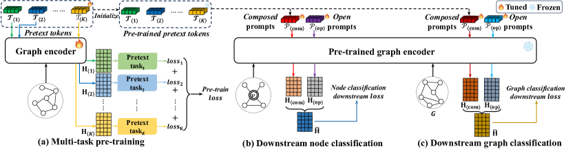
Figure 2. Overall framework of MultiGPrompt, consisting of two main stages: (a) Multi-task pre-training, and (b)/(c) Prompt-based learning for downstream few-shot tasks.

3. Preliminaries

In this work, our goal is to pre-train a graph encoder through self-supervised pretext tasks. Subsequently, the pre-trained encoder can be used for few-shot downstream tasks on graph data. We introduce related concepts and definitions in the following.

Graph. A graph is represented as $G=(V,E)$, with $V$ denoting the set of nodes and $E$ the set of edges. Equivalently, the graph can be represented by an adjacency matrix $\mathbf{A}$, such as $\mathbf{A}_{ij}=1$ iff $(v_{i},v_{j})\in E$, for any $v_{i},v_{j}\in V$. We further consider an input feature matrix for the nodes, given by $\mathbf{X}\in\mathbb{R}^{|V|\times d}$. For a node $v_{i}\in V$, its feature vector is represented as $\mathbf{x}_{i}\in\mathbb{R}^{d}$. For a dataset with multiple graphs, we use the notation $\mathcal{G}=\{G_{1},G_{2},\dots,G_{N}\}$.

Graph encoder. GNNs are popular choices of graph encoder, most of which employ a message-passing mechanism (Wu et al., 2020a). Specifically, each node in the graph aggregates messages from its neighboring nodes to update its own embedding. Multiple layers of neighborhood aggregation can be stacked, facilitating recursive message passing across the graph. Formally, let $\mathbf{H}^{l}$ be the embedding matrix of the graph at the $l$-th layer, where its $i$-th row, $\mathbf{h}_{i}^{l}$, corresponds to the embedding of node $v_{i}$. It is computed based on the embeddings from the preceding layer:

(1) $$\mathbf{H}^{l}=\textsc{MP}(\mathbf{H}^{l-1},\vec{A};\theta^{l}),$$

where $\textsc{MP}(\cdot)$ is a message passing function, $\theta^{l}$ denotes the learnable parameters of the graph encoder at the $l$-th layer. In particular, the initial embedding matrix $\mathbf{H}^{0}$, is simply given by the input feature matrix, i.e., $\mathbf{H}^{0}=\mathbf{X}$. The output after a total of $L$ layers is then $\mathbf{H}^{L}$; for brevity we simply write $\mathbf{H}$. We abstract the multi-layer encoding process as

(2) $$\mathbf{H}=\textsc{GraphEncoder}(\mathbf{X},\vec{A};\Theta),$$

where $\Theta=(\theta^{1},\ldots,\theta^{L})$ is the collection of weights across the layers.

The output embedding matrix $\mathbf{H}$ can then be fed into a loss function and optimized. In the pre-training stage, the loss can be defined with various self-supervised pretext tasks, such as DGI (Veličković et al., 2018), GraphCL (You et al., 2020) and link prediction (Liu et al., 2023a). In the downstream adaptation stage, the loss is computed based on labeled data.

Few-shot problem. For downstream tasks, we focus on few-shot learning for two graph-based tasks: node classification and graph classification. Specifically, for node classification within a graph $G=(V,E)$, let $C$ denote the set of node classes. For each node $v_{i}\in V$, its class label is $\ell_{i}\in C$. For graph classification over a set of graphs $\mathcal{G}$, we introduce $\mathcal{C}$ as the set of possible graph labels. Here, $L_{i}\in\mathcal{C}$ represents the class label for a specific graph $G_{i}\in\mathcal{G}$.

Under the few-shot setting, in either node or graph classification, there are only $m$ labeled examples (be it nodes or graphs) for each class, where $m$ is a small number (e.g., $m\leq 10$). This setup is commonly referred to as $m$-shot classification.

4. Proposed Approach

In this section, we present our proposed model MultiGPrompt.

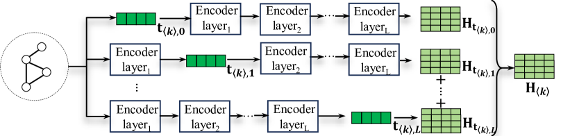
Figure 3. Application of pretext tokens to the graph encoder. $\vec{t}_{\langle k\rangle,l}$ represents the pretext token that modifies the $l$-th layer of the graph encoder for the $k$-th pretext task.

4.1. Overall Framework

We begin with the overall framework of MultiGPrompt in Fig. 2, which consists of two high-level stages: (a) multi-task pre-training on some label-free graphs, and (b)/(c) prompt-based learning for few-shot downstream tasks.

First, as shown in Fig. 2(a), our framework incorporates $K$ pretext tasks for multi-task pre-training. For the $k$-th pretext task, we employ a series of pretext tokens $\mathcal{T}_{[k]}$ to store task-specific information. The pretext tokens are learnable vectors that reformulate the input of the pretext task, which guide various pretext tasks into a synergistic integration to alleviate task interference.

Next, as shown in Fig. 2(b), we aim to transfer the pre-trained knowledge to different downstream tasks. We propose a dual-prompt mechanism with a series of composed prompts, $\mathcal{P}_{\langle\text{com}\rangle}$, and open prompts, $\mathcal{P}_{\langle\text{op}\rangle}$. The composed prompt is obtained by a learnable aggregation of the pretext tokens to leverage task-specific pre-trained knowledge. The open prompt is a learnable vector that learns global inter-task insights from the pre-trained model. Both are then used to reformulate the downstream input to the pre-trained model separately, and their respective output embeddings are combined and further fed into the downstream task loss.

4.2. Multi-task Pre-training

In this part, we discuss the first stage on multi-task pre-training. In general, any graph-based pretext tasks can be used in our framework. In our experiments, we leverage three well-known pretext tasks, namely, DGI (Veličković et al., 2018), GraphCL (You et al., 2020), and link prediction (Yu et al., 2023b). We aim to aggregate the losses of pretext tasks in a synergistic manner under the guidance of pretext tokens.

Pretext tokens. Assume we employ a total of $K$ pretext tasks for multi-task pre-training. Different pretext tasks focus on diverse aspects, and each has its unique loss function. Directly optimizing the sum of the $K$ losses leads to interference between tasks (Wu et al., 2020b; Yu et al., 2020; Wang et al., 2022c), and degrades the pre-training efficacy.

To avoid task interference, we leverage the concept of pretext tokens, which have been used to reformulate the task input in an earlier approach for pre-training language models (Wang et al., 2022c). In the context of graph, different layers of the graph encoder may have different emphasis on the representation, and thus carry variable significance to different pretext tasks. For instance, the input layer focuses on individual nodes’ features and thus are more important to node-level pretext tasks, while the hidden or output layers focus more on subgraph or graph features and thus are more important to local or graph-level tasks. Inspired by GraphPrompt+ (Yu et al., 2023b), for each pretext task, we apply a series of pretext tokens to modify the input, hidden and output layers of the graph encoder alike.

Specifically, consider a graph $G$, an encoder with a total of $L$ layers, and $K$ pretext tasks. As shown in Fig. 2(a), we put forth $K$ sets of pretext tokens, represented by $\mathcal{T}_{\langle 1\rangle},\mathcal{T}_{\langle 2\rangle},\ldots,\mathcal{T}_{\langle K\rangle}$. Each $\mathcal{T}_{\langle k\rangle}$ denotes a set of $L+1$ pretext tokens for the $k$-th pretext task, with one pretext token for each layer (including the input layer):

(3) $$\mathcal{T}_{\langle k\rangle}=\{\mathbf{t}_{\langle k\rangle,0},\mathbf{t}_{\langle k\rangle,1},\ldots,\mathbf{t}_{\langle k\rangle,L}\}.$$

That is, $\mathbf{t}_{\langle k\rangle,l}$ is a learnable vector representing the pretext token that modifies the $l$-th layer of the encoder for the $k$-th pretext task, for $1\leq k\leq K$ and $0\leq l\leq L$. This gives a total of $K\times(L+1)$ pretext tokens, and we illustrate how they are applied to modify different layers for one pretext task in Fig. 3.

Next, given any pretext token $\mathbf{t}$ in general, let $\mathbf{H}_{\mathbf{t}}$ denote the output from the graph encoder after applying the pretext token $\mathbf{t}$ to one of its layers, as follows.

(4) $$\mathbf{H_{\mathbf{t}}}=\textsc{GraphEncoder}_{\mathbf{t}}(\mathbf{X},\mathbf{A};\Theta),$$

where $\textsc{GraphEncoder}_{\mathbf{t}}(\cdot)$ indicate that one of its layers has been modified by $\mathbf{t}$. To be more specific, a pretext token $\mathbf{t}_{\langle k\rangle,l}$ will modify the $l$-th layer of the graph encoder into $\mathbf{t}_{\langle k\rangle,l}\odot\mathbf{H}^{l}$ with an element-wise multiplication, where we multiply the pretext token $\mathbf{t}_{\langle k\rangle,l}$ with each row of $\mathbf{H}^{l}$ element-wise. Subsequently, when $l<L$, the next layer will be generated as

(5) $$\mathbf{H}^{l+1}=\textsc{MP}(\mathbf{t}_{\langle k\rangle,l}\odot\mathbf{H}^{l},\vec{A};\theta^{l}).$$

Finally, for the $k$-th pretext task, we must generate one embedding matrix $\mathbf{H}_{\langle k\rangle}$ to calculate the task loss. However, with Eq. (4), each of the $L+1$ pretext tokens for the pretext task will generate its own embedding matrix. Thus, we further aggregate the $L+1$ embedding matrices to obtain the overall embedding matrix for the $k$-th task as

(6) $$\mathbf{H}_{\langle k\rangle}=\sum_{l=0}^{L}{\alpha_{l}}\mathbf{H}_{\mathbf{t}_{\langle k\rangle,l}},$$

where $\{{\alpha}_{l}:0\leq l\leq L\}$ are hyperparameters.

Pre-training loss. Equipped with a set of tailored pretext tokens for each pretext task, our multi-task pre-training can capture specific information pertinent to every pretext task in synergy. After obtaining the embedding matrix for the $k$-th pretext task in Eq. (6), we can calculate the corresponding task loss $\mathcal{L}_{\text{pre}_{\langle k\rangle}}(\mathbf{H}_{\langle k\rangle};\mathcal{T}_{\langle k\rangle},\Theta)$, where $\Theta$ represents the model weights of graph encoder. Note that $\mathbf{H}_{\langle k\rangle}$ is used to calculate the loss while $\mathcal{T}_{\langle k\rangle},\Theta$ are trainable parameters. Then, we aggregate the losses of all $K$ pretext tasks together into an overall loss for the multi-task pre-training stage:

(7) $$\mathcal{L}_{\text{pre}}(\mathcal{H};\mathcal{T},\Theta)=\sum_{k=1}^{K}\beta_{k}\mathcal{L}_{\text{pre}_{\langle k\rangle}}(\mathbf{H}_{\langle k\rangle};\mathcal{T}_{\langle k\rangle},\Theta),$$

where $\{\beta_{k}:1\leq k\leq K\}$ contains $K$ hyperparameters, $\mathcal{H}=\{\mathbf{H}_{\langle 1\rangle},\ldots,\mathbf{H}_{\langle K\rangle}\}$ represents the collection of task-specific embeddings, and $\mathcal{T}=\{\mathcal{T}_{\langle 1\rangle},\ldots,\mathcal{T}_{\langle K\rangle}\}$ denotes the collection of pretext token sets. The overall loss is optimized by updating the pretext tokens $\mathcal{T}$ and encoder weights $\Theta$. Note that the number of pretext tasks $K$ should be a small constant, with $K=3$ in our experiments.

4.3. Prompting for Downstream Tasks

To leverage not only task-specific pre-trained knowledge, but also global inter-task knowledge from the whole pre-trained model, we propose a dual-prompt mechanism with a set of composed prompts, $\mathcal{P}_{\langle\text{com}\rangle}$, and a set of open prompts, $\mathcal{P}_{\langle\text{op}\rangle}$. Composed prompts aim at transferring pretext task-specific knowledge to downstream tasks, through a learnable mixture of pretext tokens. Simultaneously, open prompts facilitate the transfer of global inter-task knowledge.

Both composed prompts and open prompts are applied to different layers of the pre-trained graph encoder in the same manner as pretext tokens, as illustrated in Fig. 3. That is, the set of composed prompts $\mathcal{P}_{\langle\text{com}\rangle}$ contains $L+1$ prompts, so does the set of open prompts $\mathcal{P}_{\langle\text{op}\rangle}$, as follows.

(8) $$\mathcal{P}_{\langle\text{com}\rangle} =\{\mathbf{p}_{{\langle\text{com}\rangle},0},\mathbf{p}_{{\langle\text{com}\rangle},1},\ldots,\mathbf{p}_{{\langle\text{com}\rangle},L}\}$$

(9) $$\mathcal{P}_{\langle\text{op}\rangle} =\{\mathbf{p}_{{\langle\text{op}\rangle},0},\mathbf{p}_{{\langle\text{op}\rangle},1},\ldots,\mathbf{p}_{{\langle\text{op}\rangle},L}\},$$

Each prompt $\mathbf{p}\in\mathcal{P}_{\langle\text{com}\rangle}$ or $\mathcal{P}_{\langle\text{op}\rangle}$ is a vector that modifies a specific layer of the pre-trained encoder. Similar to Eq. (10), let $\mathbf{H}_{\mathbf{p}}$ be the output from the pre-trained graph encoder after applying the prompt $\mathbf{p}$ to one of its layers, as follows.

(10) $$\mathbf{H_{\mathbf{p}}}=\textsc{GraphEncoder}_{\mathbf{p}}(\mathbf{X},\mathbf{A};\Theta_{\text{pre}}),$$

where $\Theta_{\text{pre}}$ contains pre-trained model weights that are frozen throughout the downstream stage. Then, define $\mathbf{H}_{\langle\text{com}\rangle}$ and $\mathbf{H}_{\langle\text{op}\rangle}$ as the final output of the pre-trained graph encoder after applying the composed prompts and open prompts, respectively. That is,

(11) $$\mathbf{H}_{\langle\text{com}\rangle}=\sum_{l=0}^{L}{\alpha_{l}}\mathbf{H}_{\mathbf{p}_{{\langle\text{com}\rangle},l}},\quad\mathbf{H}_{\langle\text{op}\rangle}=\sum_{l=0}^{L}{\alpha_{l}}\mathbf{H}_{\mathbf{p}_{{\langle\text{op}\rangle},l}},$$

where $\alpha_{l}$’s take the same values as those in Eq. (6).

In the following, we elaborate how a composed prompt and an open prompt is constructed.

Composed prompt. As given in Eq. (8), a composed prompt $\mathbf{p}_{{\langle\text{com}\rangle},l}\in\mathcal{P}_{\langle\text{com}\rangle}$ modifies the $l$-th layer of the pre-trained graph encoder, following the same fashion as Eq. (5). However, $\mathbf{p}_{{\langle\text{com}\rangle},l}$ is not directly learnable, but is instead a learnable composition of the $K$ pre-trained pretext tokens in the same layer, as given below.

(12) $$\mathbf{p}_{\langle\text{com}\rangle,l}=\textsc{Compose}(\mathbf{t}_{\langle 1\rangle,l},\mathbf{t}_{\langle 2\rangle,l},\ldots,\mathbf{t}_{\langle K\rangle,l};\Gamma),$$

where $\textsc{Compose}(\cdot)$ is a function to “compose” the $K$ pretext tokens together, such as a linear combination or neural network, and $\Gamma$ represents the learnable parameters of the function. Therefore, a composed prompt aims to learn a precise mixture of task-specific pre-trained knowledge.

Open prompt. Similar to a composed prompt, an open prompt $\mathbf{p}_{{\langle\text{op}\rangle},l}\in\mathcal{P}_{\langle\text{op}\rangle}$ modifies the $l$-th layer of the pre-trained graph encoder. Unlike the composed prompts, $\mathbf{p}_{{\langle\text{op}\rangle},l}$ is directly tuned, instead of being composed from the pretext tokens. In this way, an open prompt does not extract pre-trained knowledge specific to any pretext task, but focus on the global pre-trained model holistically.

Prompt tuning. Lastly, we generate a final embedding matrix to compute the downstream task loss. To leverage not only pretext task-specific knowledge but also global information from the pre-trained model, we incorporate the output embeddings from both the composed and open prompts given by Eq. (11). To this end, let us define an aggregation function $\textsc{Aggr}(\cdot)$, which gives the final embedding matrix $\mathbf{\tilde{H}}$ after applying the dual prompts to the pre-trained encoder, as follows.

(13) $$\mathbf{\tilde{H}}=\textsc{Aggr}(\mathbf{H}_{\langle\text{com}\rangle},\mathbf{H}_{\langle\text{op}\rangle};\Delta),$$

where $\Delta$ denotes learnable parameters of the aggregation function.

To tune the dual prompts for an arbitrary downstream task, the loss can be abstracted as $\mathcal{L}_{\text{down}}(\mathbf{\tilde{H}};\mathcal{P}_{\text{$\langle$op$\rangle$}},\Gamma,\Delta)$, where $\mathbf{\tilde{H}}$ is used to calculate the loss, and $\mathcal{P}_{\text{$\langle$op$\rangle$}},\Gamma,\Delta$ are tunable parameters associated with the prompts. Note that during prompt tuning, the pre-trained weights of the graph encoder and the pretext tokens are frozen without any tuning. Only $\mathcal{P}_{\text{$\langle$op$\rangle$}},\Gamma,\Delta$ are updated, which is much more parameter-efficient than fine-tuning the pre-trained model. Hence, our approach is particularly suitable for few-shot settings when the downstream task only offers a few labeled examples.

More concretely, in this work, we have experimented with two popular types of downstream task, namely, node classification and graph classification, and follow the same loss formulations in a previous work (Liu et al., 2023a). Details of the losses can be found in Appendix E.

5. Experiments

Table 1. Summary of datasets.

	Graphs	Graph classes	Avg. nodes	Avg. edges	Node features	Node classes	Task∗ (N/G)
Cora	1	-	2,708	5,429	1,433	7	N
Citeseer	1	-	3,327	4,732	3,703	6	N
PROTEINS	1,113	2	39.06	72.82	1	3	N, G
ENZYMES	600	6	32.63	62.14	18	3	N, G
BZR	405	2	35.75	38.36	3	-	G
COX2	467	2	41.22	43.45	3	-	G

^∗ indicates the type(s) of downstream task associated with each dataset: “N” for node classification and “G” for graph classification.

Table 2. Accuracy evaluation on few-shot node and graph classification.

Methods	Node classification				Graph classification
	Cora	Citeseer	PROTEINS	ENZYMES	BZR	COX2	PROTEINS	ENZYMES
GCN	28.57 $\pm$ 5.07	31.27 $\pm$ 04.53	43.31 $\pm$ 09.35	48.08 $\pm$ 04.71	56.33 $\pm$ 10.40	50.95 $\pm$ 23.48	50.56 $\pm$ 03.01	17.10 $\pm$ 3.53
GAT	28.40 $\pm$ 6.25	30.76 $\pm$ 05.40	31.79 $\pm$ 20.11	35.32 $\pm$ 18.72	50.69 $\pm$ 23.66	50.58 $\pm$ 26.16	50.59 $\pm$ 12.43	16.80 $\pm$ 2.97
DGI/InfoGraph	54.11 $\pm$ 9.60	45.00 $\pm$ 09.19	45.22 $\pm$ 11.09	48.05 $\pm$ 14.83	52.57 $\pm$ 18.14	54.62 $\pm$ 15.36	48.21 $\pm$ 12.35	21.69 $\pm$ 5.98
GraphCL	51.96 $\pm$ 9.43	43.12 $\pm$ 09.61	46.15 $\pm$ 10.94	48.88 $\pm$ 15.98	54.11 $\pm$ 16.63	54.29 $\pm$ 17.31	53.69 $\pm$ 11.92	21.57 $\pm$ 5.20
GPPT	15.37 $\pm$ 4.51	21.45 $\pm$ 03.45	35.15 $\pm$ 11.40	35.37 $\pm$ 09.37	-	-	-	-
GraphPrompt	54.25 $\pm$ 9.38	45.34 $\pm$ 10.53	47.22 $\pm$ 11.05	53.54 $\pm$ 15.46	54.60 $\pm$ 10.53	54.35 $\pm$ 14.78	54.73 $\pm$ 08.87	25.06 $\pm$ 7.56
MultiGPrompt	57.72 $\pm$ 9.94	54.74 $\pm$ 11.57	48.09 $\pm$ 11.49	54.47 $\pm$ 15.36	60.07 $\pm$ 12.48	56.17 $\pm$ 12.84	56.02 $\pm$ 08.27	26.63 $\pm$ 6.22

Results are reported in percent. The best method is bolded and the runner-up is underlined.

In this section, we undertake comprehensive experiments across six benchmark datasets, to evaluate the efficacy of the proposed MultiGPrompt on few-shot node and graph classification tasks. The datasets and code are available.

5.1. Experimental Setup

Datasets. We employ six benchmark datasets for evaluation. (1) Cora (McCallum et al., 2000) and (2) Citeseer (Sen et al., 2008) are both citation graphs. Each of them involves a single graph, where the nodes are publications and the edges are citations. As with previous work (Kipf and Welling, 2017; Veličković et al., 2018), we treat their edges as undirected. (3) PROTEINS (Borgwardt et al., 2005) comprises 1,113 protein graphs. Each node signifies a secondary structure, and the edges represent the neighboring relations between the structures, within the amino-acid sequence or in 3D space. (4) ENZYMES (Wang et al., 2022a), (5) BZR (Rossi and Ahmed, 2015), and (6) COX2 (Rossi and Ahmed, 2015) are collections of molecular graphs, describing the structures of 600 enzymes from the BRENDA enzyme database, 405 ligands pertinent to the benzodiazepine receptor, and 467 cyclooxygenase-2 inhibitors, respectively.

We summarize the characteristics of these datasets in Table 1, and provide a comprehensive description in Appendix A.

Baselines. We evaluate MultiGPrompt against a spectrum of state-of-the-art methods that can be broadly grouped into three primary categories, as follows.

(1) End-to-end graph neural networks: These include GCN (Kipf and Welling, 2017) and GAT (Veličković et al., 2018), which are trained in a supervised manner using the downstream labels directly, without pre-training.

(2) Graph pre-training models: We compare to DGI/InfoGraph (Veličković et al., 2018; Sun et al., 2019), and GraphCL (You et al., 2020). Specifically, the pre-training stage only uses label-free graphs, and the downstream adaptation stage further trains a classifier using few-shot labels while freezing the pre-trained weights.

(3) Graph prompt-based learning: GPPT (Sun et al., 2022) and GraphPrompt (Liu et al., 2023a) are included under this umbrella. They first leverage link prediction during pre-training, and unify downstream tasks into a common template as the pretext task. Both of them utilizes a single pretext task, and subsequently a single type of prompt in downstream adaptation. Note that GPPT is purposely designed to work with the downstream task of node classification, and cannot be directly applied to graph classification. Hence, in our experiments, we only employ GPPT for node classification.

We present more details of the baselines in Appendix B. It is worth noting that certain few-shot methodologies on graphs, such as Meta-GNN (Zhou et al., 2019), AMM-GNN (Wang et al., 2020), RALE (Liu et al., 2021a), VNT (Tan et al., 2023), and ProG (Sun et al., 2023), hinge on the meta-learning paradigm (Finn et al., 2017), requiring an additional set of labeled base classes in addition to the few-shot classes. Hence, they are not comparable to our framework.

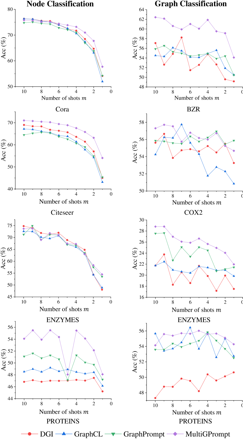
Figure 4. Impact of shots on node and graph classification.

Setup of downstream tasks. We conduct two types of downstream task, i.e., node classification and graph classification. The tasks are configured in a $m$-shot classification setup, i.e., for each class, we randomly draw $m$ examples (nodes or graphs) as supervision. In our main results, we use $m=1$ for node classification, and $m=5$ for graph classification. Nevertheless, we also vary the number of shots for $1\leq m\leq 10$, to show the robustness of our approach under different settings.

We repeat the sampling 100 times to construct 100 $m$-shot tasks for node classification as well as graph classification. For each task, we run with five different random seeds. Thus, there are a total of 500 results per type of task, and we report the average and standard deviation over the 500 results. Since the $m$-shot tasks are balanced classification, we simply evaluate the performance using accuracy, in line with previous works (Wang et al., 2020; Liu et al., 2021a, 2023a).

Note that, for datasets with both node and graph classification tasks, i.e., PROTEINS and ENZYMES, we only pre-train the graph encoder once for each dataset. Subsequently, we employ the same pre-trained model for both types of downstream task.

Parameter settings. For all baselines, we reuse the original authors’ code and their recommended settings, and further tune their hyper-parameters to ensure competitive performance. A more granular description of the implementations and settings, for both the baselines and our MultiGPrompt, is furnished in Appendix C.

5.2. Few-shot Performance Evaluation

We first report the performance of one-shot node classification and five-shot graph classification. Next, we study the impact of varying number of shots on the performance.

One-shot node classification. The results are presented in Table 2. We make the following observations. First, MultiGPrompt surpasses all baselines on all four datasets, indicating its advantage in the overall strategy of multi-task pre-training. We will further conduct a series of ablation studies in Sect. 5.3 to evaluate the importance of specific designs. Second, pre-training methods (DGI/InfoGraph, GraphCL) generally outperform supervised methods (GCN, GAT), as the former group leverage a pre-trained model, which highlights the importance of acquiring general knowledge from label-free graphs. Lastly, “pre-train, prompt” methods, such as GraphPrompt and our MultiGPrompt, can further outperform the pre-training approaches without prompts, demonstrating the advantage of prompt-based learning epsecially in few-shot settings.

Five-shot graph classification. We further conduct graph classification and also report the results in Table 2. The trends on graph classification are mostly consistent with those observed in the node classification results, underpinning the generality of MultiGPrompt (and more broadly, the paradigm of prompt-based learning) across both node- and graph-level tasks.

Impact of different shots. To delve deeper into the robustness of MultiGPrompt in different learning setups, we vary the the number of shots $m$ for both node and graph classification tasks. We present the performance of MultiGPrompt against a line-up of competitive baselines in Fig. 4, and make several observations.

First, MultiGPrompt largely performs better than the baselines, especially in low-shot settings (e.g., $m\leq 5$) when very limited labeled data are given. Second, when more shots are given (e.g., $m>5$), all methods perform better in general, which is expected. Nonetheless, the performance of MultiGPrompt remains competitive, if not better. Note that on certain datasets such as PROTEINS, the performance of most methods suffer from large variances. One potential reason is it has least node features (see Table 1), which exacerbate the difficulty of few-shot classification. Additionally, the graphs in PROTEINS tend to vary in size more significantly than other datasets, which may also contribute to the larger variances in the performance. Despite these issues, the performance of MultiGPrompt is still more robust than other methods.

Table 3. Ablation study on prompt design for multi-task pre-training.

Methods	Pretext	Composed	Open	Node classification				Graph classification
	token	prompt	prompt	Cora	Citeseer	PROTEINS	ENZYMES	BZR	COX2	PROTEINS	ENZYMES
Variant 1	$\times$	$\times$	$\times$	56.58	50.69	46.48	48.04	49.63	54.35	55.72	21.07
Variant 2	$\times$	$\times$	$\checkmark$	56.54	53.08	47.79	51.09	47.56	54.89	55.61	24.23
Variant 3	$\checkmark$	$\times$	$\times$	45.00	52.36	45.11	50.55	57.14	54.43	55.67	21.06
Variant 4	$\checkmark$	$\times$	$\checkmark$	56.59	50.63	47.64	50.52	57.52	55.21	55.12	24.30
Variant 5	$\checkmark$	$\checkmark$	$\times$	56.83	53.72	47.50	53.11	55.71	53.04	55.15	23.33
MultiGPrompt	$\checkmark$	$\checkmark$	$\checkmark$	57.72	54.74	48.09	54.47	60.07	56.17	56.02	26.63

Results are evaluated using classification accuracy, reported in percent. The best variant is bolded.

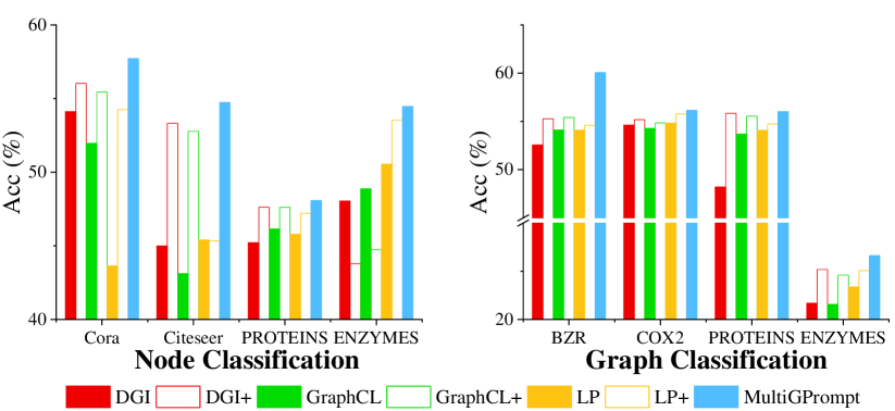
Figure 5. Ablation study on pretext tasks.

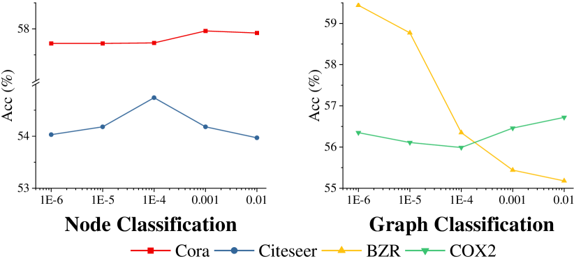
Figure 6. Impact of hyperparameter $\alpha_{0}$.

5.3. Ablation study

To thoroughly understand the impact of each component within MultiGPrompt, we conduct two ablation analyses. The initial analysis studies the effect of multiple pretext tasks, and the second analysis contrasts MultiGPrompt with variants employing different prompts.

We start with three basic variants that only utilize a single pretext task: using only DGI/InfoGraph (DGI), GraphCL, and link prediction (LP). These three basic variants employ a classifier during downstream fine-tuning, without prompting. We further compare three more advanced variants, namely, DGI+, GraphCL+ and LP+, which has the exact same architecture and dual-prompt design as the full model MultiGPrompt, but only utilize one pretext task. Referring to Fig. 5, we observe that MultiGPrompt consistently outperforms all variants using a single pretext task, with or without prompts, which underscores the value of leveraging multiple pretext tasks.

Next, for multi-task pre-training, we investigate several variants of MultiGPrompt by removing key designs in our dual prompts, including the use of pretext tokens, composed prompts and open prompts. These variants and their corresponding results are tabulated in Table 3. The outcomes corroborate that each individual design is instrumental, as analyzed below. First, employing pretext tokens and composed prompts is beneficial. Notably, Variant 5 typically outperforms Variants 1 and 3, which do not utilize a composed prompt. However, solely employing pretext tokens, as in Variant 3, does not give a stable improvement over Variant 1, implying that the pretext tokens work the best in conjunction with the composed prompts. (Note that composed prompts are built upon the pretext tokens and cannot work alone without the latter.) Second, omitting open prompts leads to diminished performance, as evident in the higher accuracy of Variants 2 and 4 against Variants 1 and 3. This shows the importance of leveraging global inter-task knowledge via open prompts. Lastly, the dual-prompt design, comprising both composed and open prompts, proves beneficial, helping MultiGPrompt achieve the most optimal performance.

5.4. Further Model Analysis

We conduct further analysis related to the hyperparameter selection and parameter efficiency of MultiGPrompt.

Hyperparameter selection. We assess the impact of $\alpha^{l}$’s, used in Eqs. (6) and (11), which adjust the balance between the pretext tokens or prompts across different layers. In our experiments, we only employ one message-passing layer in the graph encoder, i.e., $L=1$, giving us two hyperparameters $\alpha_{0}$ and $\alpha_{1}$. Note that $\alpha_{0}$ controls the importance of prompts on the input layer, whereas $\alpha_{1}$ controls that of the output layer of the graph encoder. We fix $\alpha_{1}=1$ while varying $\alpha_{0}$, and illustrate its impact in Fig. 6.

We observe that, for node classification, as $\alpha_{0}$ increases, the accuracy initially rises. Upon reaching a peak, the accuracy begins to gradually decline with further increases in $\alpha_{0}$. In contrast, for graph classification, it appears to follow a different trend. As $\alpha_{0}$ decreases, accuracy tends to improve. Overall, node classification tasks favor somewhat larger $\alpha_{0}$, while graph classification tasks lean toward smaller $\alpha_{0}$. This phenomenon could be attributed to the differences in node classification and graph classification. Being a node-level task, node classification naturally focuses more on the node’s input features, while graph classification is affected more by the global graph representation. Hence, node classification would place a higher weight on the input layer as controlled by $\alpha_{0}$, whereas graph classification would weigh the output layer more, which captures comparatively more global information across the graph after undergoing the message-passing layers.

Table 4. Comparison of the number of tunable parameters during the downstream adaptation stage.

Methods	Node classification		Graph classification
	Cora	Citeseer	BZR	COX2
GCN	368,640	949,504	1,280	1,280
DGI/InfoGraph	1,792	1,536	768	768
GraphCL	1,792	1,536	768	768
GraphPrompt	256	256	256	256
MultiGPrompt	522	522	522	522

Parameters efficiency. Lastly, we analyze the parameter efficiency of our approach MultiGPrompt in comparison to other representative methods. Specifically, we calculate the number of parameters that require updating or tuning during the downstream adaptation stage, and list the statistics in Table 4. For GCN, as it is trained end-to-end, all the model weights have to be updated, leading to the worst parameter efficiency. For DGI/InfoGraph and GraphCL, we only update the downstream classifier without updating the pre-trained model, resulting in a significant reduction in the number of tunable parameters. Finally, prompt-based methods GraphPrompt and MultiGPrompt are the most parameter efficient, as prompts are light-weight and contain fewer parameters than a typical classifier such as a fully connected layer. Note that, due to our dual-prompt design, MultiGPrompt needs to update more parameters than GraphPrompt in the downstream adaptation stage. However, the increase in the tunable parameters downstream is still insignificant compared to updating the classifier or the full model weights, and thus does not present a fundamental problem.

6. Conclusions

In this paper, we explored multi-task pre-training and prompting on graphs, aiming to encompass a comprehensive range of knowledge from diverse pretext tasks. Our proposed approach MultiGPrompt designs a series of pretext tokens to leverage multiple pretext tasks in a synergistic manner. Moreover, we introduced a dual-prompt mechanism with both composed prompts and open prompts, to utilize both pretext task-specific and global inter-task knowledge. Finally, we conducted extensive experiments on six public datasets and demonstrated that MultiGPrompt significantly outperforms various state-of-the-art baselines.

Appendices

A. Further Descriptions of Datasets

We provide further details of the datasets.

(1) Cora (McCallum et al., 2000) comprises 2,708 scientific publications, each categorized into one of seven classes. The citation network encompasses 5,429 links. Every publication in the dataset is depicted by a 0/1-valued word vector, indicating the absence/presence of the corresponding word from the dictionary, which consists of 1433 unique words.

(2) Citeseer (Sen et al., 2008) is composed of 3,312 scientific publications, each categorized into one of six classes. The citation network entails 4,732 links. Each publication in the dataset is characterized by a 0/1-valued word vector, indicating the absence/presence of the corresponding word from the dictionary, which encompasses 3,703 unique words.

(3) PROTEINS (Borgwardt et al., 2005) encompasses a collection of protein graphs, embodying various attributes including the amino acid sequence, conformation, structure, and distinctive features such as active sites of the proteins. In this collection, each node signifies the secondary structures, whereas each edge represents the neighboring relation either within the amino-acid sequence or in 3D space. The nodes are classified into three categories, while the graphs are divided into two classes.

(4) ENZYMES${}^{\ref{footnote:data}}$ (Wang et al., 2022a) constitutes a dataset comprising 600 enzymes, meticulously collected from the BRENDA enzyme database. These enzymes are meticulously categorized into 6 distinct classes in accordance with their top-level EC enzyme classification.

(5) BZR${}^{\ref{footnote:data}}$ (Rossi and Ahmed, 2015) encompasses a collection of 405 ligands, each associated with the benzodiazepine receptor and graphically represented as individual entities. The entire ligand set is bifurcated into 2 distinct categories.

(6) COX2${}^{\ref{footnote:data}}$ (Rossi and Ahmed, 2015) encompasses a dataset that includes 467 molecular structures, specifically of cyclooxygenase-2 inhibitors, wherein each node symbolizes an atom and each edge represents the chemical bond—be it single, double, triple, or aromatic—between atoms. The entirety of the molecules is categorized into two classes.

We conduct node classification on Cora, Citeseer, PROTEINS, and ENZYMES, by aggregating the graphs within a dataset into a larger graph. Additionally, graph classification is conducted on PROTEINS, COX2, ENZYMES, and BZR.

B. Further Descriptions of Baselines

In this section, we present more details for the baselines used in our experiments.

(1) End-to-end Graph Neural Networks

• GCN (Kipf and Welling, 2017): GCN employs a mean-pooling-based neighborhood aggregation approach to process messages from adjacent nodes.

• GAT (Veličković et al., 2018): GAT also leverages neighborhood aggregation for end-to-end node representation learning. However, during the aggregation process, it allocates varied weights to neighboring nodes through an attention mechanism.

(2) Graph Pre-training Models

• DGI (Veličković et al., 2018): DGI operates as a self-supervised pre-training method. It is predicated on the maximization of mutual information, aiming to enhance the consistency between locally augmented instances and their global counterparts.

• InfoGraph (Sun et al., 2019): Expanding upon DGI, InfoGraph is centered on graph-level tasks, aiming to maximize the alignment between node and graph embeddings.

• GraphCL (You et al., 2020): GraphCL leverages a variety of graph augmentations for self-supervised learning, tapping into various intrinsic properties of the graphs for pre-training.

(3) Graph Prompt Models

• GPPT (Sun et al., 2022): GPPT employs a GNN model, pre-trained on a link prediction task. A prompt module is designed to facilitate the downstream node classification task, which is converted to a link prediction format.

• GraphPrompt (Liu et al., 2023a): GraphPrompt employs subgraph similarity as a mechanism to unify different pretext and downstream tasks, including link prediction, node classification, and graph classification. A learnable prompt is subsequently tuned for each downstream task.

C. Implementation Details

Details of baselines. For all the baseline models, we utilize the codes officially disseminated by their respective authors. Each model is tuned in accordance with the settings recommended in their respective literature to ascertain optimal performance.

For the baseline GCN (Kipf and Welling, 2017), we employ a 3-layer architecture, and set the hidden dimensions to 256. For GAT (Veličković et al., 2018), we employ a 2-layer architecture and set the hidden dimension to 64. Additionally, we apply 8 attention heads in the first GAT layer.

For DGI (Veličković et al., 2018), we utilize a 1-layer GCN as the base model and set the hidden dimensions to 256. Additionally, we employ prelu as the activation function. For GraphCL (You et al., 2020), a 1-layer GCN is also employed as its base model, with the hidden dimensions set to 256. Specifically, we select edge dropping as the augmentations, with a default augmentation ratio of 0.2.

For GPPT (Sun et al., 2022), we utilize a 2-layer GraphSAGE as its base model, setting the hidden dimensions to 256. For base GraphSAGE, we also employ a mean aggregator. For GraphPrompt (Liu et al., 2023a), a 3-layer GCN is used as the base model for all datasets, with the hidden dimensions set to 256.

Details of MultiGPrompt. For our proposed MultiGPrompt, we utilize a 1-layer GCN as the base model for all datasets, with the hidden dimensions set to 256. We set $\alpha_{0}=0.0001$ for node classification tasks, while setting $\alpha_{0}=0$ for graph classification tasks. Meanwhile, $\alpha_{1}$ is set to $1$ for both tasks. The parameters $\beta_{1}$, $\beta_{2}$, and $\beta_{3}$ are set to $0.9$, $0.9$, and $0.1$, respectively.

D. Pretext Tasks

In our experiments, we employ three pretext tasks, i.e., DGI (Veličković et al., 2018), GraphCL (You et al., 2020) and link prediction (Liu et al., 2023a). Consider a pretext task $k$ and a graph $G$. $\mathcal{T}_{\langle k\rangle}$ serves as the pretext tokens for the task $k$. Define $\vec{h}_{{\langle k\rangle},v}$, a row of $\vec{H}_{\langle k\rangle}$, as node $v$’s representation specific to task $k$. Further let $\vec{h}_{\langle k\rangle,G}$ denote the representation of $G$ for task $k$, which is given by

(14) $$\mathbf{h}_{{\langle k\rangle},G}=\textsc{Readout}(\vec{H}_{{\langle k\rangle}}).$$

Then, the loss function of DGI can be expressed as follows.

(15) $$\begin{aligned} \sum_{G\in\mathcal{X}_{\text{pre}}}\frac{1}{|\mathcal{A}_{G}|+|\mathcal{B}_{G}|}(\sum_{a\in\mathcal{A}_{G}}\log[\text{sim}(\vec{h}_{\langle\text{DGI}\rangle,a},\vec{h}_{{\langle\text{DGI}\rangle},G})]+\\ \sum_{b\in\mathcal{B}_{G}}\log[1-\text{sim}(\vec{h}_{{\langle\text{DGI}\rangle},b},\vec{h}_{{\langle\text{DGI}\rangle},G})]),\end{aligned}$$

where $\mathcal{X}_{\text{pre}}$ is a set of pre-training graphs, and $\mathcal{A}_{G},\mathcal{B}_{G}$ represent the set of positive and negative instances for $G$, respectively.

Similarly, the pre-training loss for GraphCL (abbreviated as GCL) can be formulated as follows.

(16) $$-\sum_{G\in\mathcal{X}_{\text{pre}}}\ln\frac{\exp(\text{sim}(\mathbf{h}_{\langle\text{GCL}\rangle,a\in\mathcal{A}_{G}},\mathbf{h}_{{\langle\text{GCL}\rangle},v\in V_{G}})/\tau)}{\sum_{b\in\mathcal{B}_{G}}\exp(\text{sim}(\mathbf{h}_{{\langle\text{GCL}\rangle},b},\mathbf{h}_{\langle\text{GCL}\rangle,v\in V_{G}})/\tau)},$$

where $V_{G}$ denotes the set of nodes in graph $G$, and $\tau$ is a temperature hyperparameter.

Finally, let the $1$-hop subgraph of node $v$ be denoted as $S_{v}$. Then, the pre-training loss for link prediction (abbreviated as LP) can be formulated as follows.

(17) $$-\sum_{(v,a,b)\in\mathcal{X}_{\text{pre}}}\ln\frac{\exp(\text{sim}(\mathbf{h}_{{\langle\text{LP}\rangle},S_{v}},\mathbf{h}_{{\langle\text{LP}\rangle},S_{a}})/\tau)}{\sum{u\in\{a,b\}}\exp(\text{sim}(\mathbf{h}_{{\langle\text{LP}\rangle},S_{v}},\mathbf{h}_{{\langle\text{LP}\rangle},S_{b}})/\tau)},$$

where $\vec{h}_{{\langle\text{LP}\rangle},S_{v}}$ serves as the vector representation of $S_{v}$, which is calculated through a readout similar to Eq. (14). $\mathcal{X}_{\text{pre}}$ denotes the set of tuples sampled for link prediction (Liu et al., 2023a), where a tuple $(v,a,b)$ implies that $(v,a)$ is an edge (i.e., a positive example) and $(v,b)$ is not an edge (i.e., a negative example).

E. Prompt Tuning Loss

We resort to a loss based on node or graph similarity. Consider an node or graph classification task with a labeled training set $\mathcal{D}_{\text{down}}=\{(x_{1},y_{1}),(x_{2},y_{2}),\ldots\}$, where $x_{i}$ is either a node or a graph, and $y_{i}\in Y$ is $x_{i}$’s class label from a set of classes $Y$. Then, the prompt tuning loss is defined as $\mathcal{L}_{\text{down}}(\mathbf{\tilde{H}};\mathcal{P}_{\text{op}},\Gamma,\Delta)=$

(18) $$-\sum_{(x_{i},y_{i})\in\mathcal{D}_{\text{down}}}\ln\frac{\exp\left(\frac{1}{\tau}\text{sim}(\mathbf{\tilde{h}}_{x_{i}},\overline{\mathbf{\tilde{h}}}_{y_{i}})\right)}{\sum_{y\in Y}\exp\left(\frac{1}{\tau}\text{sim}(\mathbf{\tilde{h}}_{x_{i}},\overline{\mathbf{\tilde{h}}}_{y})\right)},$$

where $\mathbf{\tilde{h}}_{x_{i}}$ denotes the final embedding of node/graph $x_{i}$, and $\overline{\mathbf{\tilde{h}}}_{y}$ is the prototype embedding of class $y$, which is the mean representation of the training instances of class $y$. $\tau$ is a temperature hyperparameter. More specifically, for a node instance $v$, $\mathbf{\tilde{h}}_{v}$ is a row of $\vec{\tilde{H}}$; for a graph instance $G$, $\mathbf{\tilde{h}}_{G}=\textsc{Readout}(\vec{\tilde{H}})$.

F. Cross-Dataset Adaptation

Table 5. Accuracy evaluation on few-shot graph classification, in same- or cross-dataset scenarios.

Pretext	BZR		COX2
Downstream	BZR	COX2	BZR	COX2
InfoGraph	52.57$\pm$18.14	53.71$\pm$16.07	52.44$\pm$24.49	54.62$\pm$15.36
GraphCL	54.11$\pm$16.63	51.60$\pm$16.78	53.61$\pm$24.38	54.29$\pm$17.31
GraphPrompt	54.60$\pm$10.53	55.48$\pm$11.36	53.78$\pm$11.92	54.34$\pm$14.78
MultiGPrompt	60.07$\pm$12.48	55.81$\pm$13.08	59.58$\pm$13.03	56.17$\pm$12.84

To further analyze the robustness of MultiGPrompt, we conduct additional experiments using different datasets for pre-training and downstream tasks, in a so-called “cross-dataset” scenario. Specifically, we select the BZR and COX2 datasets, as they possess the same node attributes, which means the model pre-trained on one dataset can be directly applied to the other dataset. We respectively employ BZR and COX2 for pre-training, and perform downstream adaptation on these two datasets.

The results for 5-shot graph classification are reported in Table 5, for same-dataset scenarios (i.e., both pretext and downstream tasks on the same dataset), as well as cross-dataset scenarios (i.e., pretext tasks on BZR and downstream tasks on COX2, or vice versa). We observe that MultiGPrompt consistently surpasses other baselines even in the cross-dataset scenarios, demonstrating the robustness of the overall multi-task pre-training and prompting strategy. Moreover, the performance of MultiGPrompt in the cross-dataset setting shows negligible decrease from the performance in the same-dataset setting. This further demonstrates the efficacy of MultiGPrompt in adapting to diverse datasets.

References

- (1)
- Agarwal et al. (2022) Vibhor Agarwal, Sagar Joglekar, Anthony P Young, and Nishanth Sastry. 2022. GraphNLI: A Graph-based Natural Language Inference Model for Polarity Prediction in Online Debates. In the ACM Web Conference. 2729–2737.
- Anonymous (2024a) Anonymous. 2024a. Graph Lottery Ticket Automated. In International Conference on Learning Representations.
- Anonymous (2024b) Anonymous. 2024b. NuwaDynamics: Discovering and Updating in Causal Spatio-Temporal Modeling. In International Conference on Learning Representations.
- Bao et al. (2022) Hangbo Bao, Li Dong, Songhao Piao, and Furu Wei. 2022. BEiT: BERT Pre-Training of Image Transformers. In International Conference on Learning Representations.
- Borgwardt et al. (2005) Karsten M Borgwardt, Cheng Soon Ong, Stefan Schönauer, SVN Vishwanathan, Alex J Smola, and Hans-Peter Kriegel. 2005. Protein function prediction via graph kernels. Bioinformatics 21, suppl_1 (2005), i47–i56.
- Brown et al. (2020) Tom Brown, Benjamin Mann, Nick Ryder, Melanie Subbiah, Jared D Kaplan, Prafulla Dhariwal, Arvind Neelakantan, Pranav Shyam, Girish Sastry, Amanda Askell, et al. 2020. Language models are few-shot learners. Advances in neural information processing systems 33 (2020), 1877–1901.
- Devlin et al. (2018) Jacob Devlin, Ming-Wei Chang, Kenton Lee, and Kristina Toutanova. 2018. BERT: Pre-training of deep bidirectional transformers for language understanding. arXiv preprint arXiv:1810.04805 (2018).
- Dong et al. (2019) Li Dong, Nan Yang, Wenhui Wang, Furu Wei, Xiaodong Liu, Yu Wang, Jianfeng Gao, Ming Zhou, and Hsiao-Wuen Hon. 2019. Unified language model pre-training for natural language understanding and generation. Advances in Neural Information Processing Systems 32 (2019).
- Dong et al. (2024) Xue Dong, Xuemeng Song, Minghui Tian, and Linmei Hu. 2024. Prompt-based and weak-modality enhanced multimodal recommendation. Information Fusion 101 (2024).
- Erhan et al. (2010) Dumitru Erhan, Aaron Courville, Yoshua Bengio, and Pascal Vincent. 2010. Why does unsupervised pre-training help deep learning?. In International Conference on Artificial Intelligence and Statistics. 201–208.
- Fan et al. (2023) Ziwei Fan, Zhiwei Liu, Shelby Heinecke, Jianguo Zhang, Huan Wang, Caiming Xiong, and Philip S Yu. 2023. Zero-shot Item-based Recommendation via Multi-task Product Knowledge Graph Pre-Training. arXiv preprint arXiv:2305.07633 (2023).
- Fang et al. (2023a) Junfeng Fang, Wei Liu, Yuan Gao, Zemin Liu, An Zhang, Xiang Wang, and Xiangnan He. 2023a. Evaluating Post-hoc Explanations for Graph Neural Networks via Robustness Analysis. Advances in Neural Information Processing Systems 36 (2023).
- Fang et al. (2023b) Junfeng Fang, Xiang Wang, An Zhang, Zemin Liu, Xiangnan He, and Tat-Seng Chua. 2023b. Cooperative Explanations of Graph Neural Networks. In ACM International Conference on Web Search and Data Mining. 616–624.
- Fang et al. (2022) Taoran Fang, Yunchao Zhang, Yang Yang, Chunping Wang, and Lei Chen. 2022. Universal Prompt Tuning for Graph Neural Networks. arXiv preprint arXiv:2209.15240 (2022).
- Finn et al. (2017) Chelsea Finn, Pieter Abbeel, and Sergey Levine. 2017. Model-agnostic meta-learning for fast adaptation of deep networks. In International Conference on Machine Learning. 1126–1135.
- Gong et al. (2021) Haifan Gong, Guanqi Chen, Sishuo Liu, Yizhou Yu, and Guanbin Li. 2021. Cross-modal self-attention with multi-task pre-training for medical visual question answering. In International Conference on Multimedia Retrieval. 456–460.
- Hamilton et al. (2017) Will Hamilton, Zhitao Ying, and Jure Leskovec. 2017. Inductive representation learning on large graphs. Advances in Neural Information Processing Systems 30 (2017), 1024–1034.
- Hu et al. (2019) Weihua Hu, Bowen Liu, Joseph Gomes, Marinka Zitnik, Percy Liang, Vijay Pande, and Jure Leskovec. 2019. Strategies for pre-training graph neural networks. arXiv preprint arXiv:1905.12265 (2019).
- Hu et al. (2020c) Weihua Hu, Bowen Liu, Joseph Gomes, Marinka Zitnik, Percy Liang, Vijay Pande, and Jure Leskovec. 2020c. Strategies for Pre-training Graph Neural Networks. In International Conference on Learning Representations.
- Hu et al. (2020b) Ziniu Hu, Yuxiao Dong, Kuansan Wang, Kai-Wei Chang, and Yizhou Sun. 2020b. GPT-GNN: Generative pre-training of graph neural networks. In ACM SIGKDD International Conference on Knowledge Discovery & Data Mining. 1857–1867.
- Hu et al. (2020a) Ziniu Hu, Yuxiao Dong, Kuansan Wang, and Yizhou Sun. 2020a. Heterogeneous graph transformer. In the ACM Web Conference. 2704–2710.
- Khattak et al. (2023) Muhammad Uzair Khattak, Hanoona Abdul Rasheed, Muhammad Maaz, Salman H. Khan, and Fahad Shahbaz Khan. 2023. MaPLe: Multi-modal Prompt Learning. In IEEE/CVF Conference on Computer Vision and Pattern Recognition. 19113–19122.
- Kipf and Welling (2017) Thomas N Kipf and Max Welling. 2017. Semi-supervised classification with graph convolutional networks. In ICLR.
- Li et al. (2024a) Shengrui Li, Xueting Han, and Jing Bai. 2024a. AdapterGNN: Efficient Delta Tuning Improves Generalization Ability in Graph Neural Networks. In AAAI Conference on Artificial Intelligence.
- Li et al. (2023) Yibo Li, Xiao Wang, Hongrui Liu, and Chuan Shi. 2023. A generalized neural diffusion framework on graphs. arXiv preprint arXiv:2312.08616 (2023).
- Li et al. (2024b) Yibo Li, Xiao Wang, Yujie Xing, Shaohua Fan, Ruijia Wang, Yaoqi Liu, and Chuan Shi. 2024b. Graph Fairness Learning under Distribution Shifts. arXiv preprint arXiv:2401.16784 (2024).
- Liu et al. (2021b) Pengfei Liu, Weizhe Yuan, Jinlan Fu, Zhengbao Jiang, Hiroaki Hayashi, and Graham Neubig. 2021b. Pre-train, prompt, and predict: A systematic survey of prompting methods in natural language processing. arXiv preprint arXiv:2107.13586 (2021).
- Liu et al. (2023b) Pengfei Liu, Weizhe Yuan, Jinlan Fu, Zhengbao Jiang, Hiroaki Hayashi, and Graham Neubig. 2023b. Pre-train, prompt, and predict: A systematic survey of prompting methods in natural language processing. Comput. Surveys 55, 9 (2023), 1–35.
- Liu et al. (2021a) Zemin Liu, Yuan Fang, Chenghao Liu, and Steven CH Hoi. 2021a. Relative and absolute location embedding for few-shot node classification on graph. In AAAI Conference on Artificial Intelligence. 4267–4275.
- Liu et al. (2023a) Zemin Liu, Xingtong Yu, Yuan Fang, and Xinming Zhang. 2023a. GraphPrompt: Unifying pre-training and downstream tasks for graph neural networks. In the ACM Web Conference. 417–428.
- Lu et al. (2021) Yuanfu Lu, Xunqiang Jiang, Yuan Fang, and Chuan Shi. 2021. Learning to pre-train graph neural networks. In AAAI Conference on Artificial Intelligence, Vol. 35. 4276–4284.
- McCallum et al. (2000) Andrew Kachites McCallum, Kamal Nigam, Jason Rennie, and Kristie Seymore. 2000. Automating the construction of internet portals with machine learning. Information Retrieval 3 (2000), 127–163.
- Mormont et al. (2020) Romain Mormont, Pierre Geurts, and Raphaël Marée. 2020. Multi-task pre-training of deep neural networks for digital pathology. IEEE Journal of Biomedical and Health Informatics 25, 2 (2020), 412–421.
- Qiu et al. (2020) Jiezhong Qiu, Qibin Chen, Yuxiao Dong, Jing Zhang, Hongxia Yang, Ming Ding, Kuansan Wang, and Jie Tang. 2020. GCC: Graph contrastive coding for graph neural network pre-training. In ACM SIGKDD International Conference on Knowledge Discovery & Data Mining. 1150–1160.
- Qu et al. (2023) Liang Qu, Ningzhi Tang, Ruiqi Zheng, Quoc Viet Hung Nguyen, Zi Huang, Yuhui Shi, and Hongzhi Yin. 2023. Semi-decentralized Federated Ego Graph Learning for Recommendation. arXiv preprint arXiv:2302.10900 (2023).
- Rossi and Ahmed (2015) Ryan A. Rossi and Nesreen K. Ahmed. 2015. The Network Data Repository with Interactive Graph Analytics and Visualization. In AAAI. 4292–4293.
- Sen et al. (2008) Prithviraj Sen, Galileo Namata, Mustafa Bilgic, Lise Getoor, Brian Galligher, and Tina Eliassi-Rad. 2008. Collective classification in network data. AI Magazine 29, 3 (2008), 93–93.
- Su et al. (2021) Yixuan Su, Lei Shu, Elman Mansimov, Arshit Gupta, Deng Cai, Yi-An Lai, and Yi Zhang. 2021. Multi-task pre-training for plug-and-play task-oriented dialogue system. arXiv preprint arXiv:2109.14739 (2021).
- Sun et al. (2019) Fan-Yun Sun, Jordan Hoffmann, Vikas Verma, and Jian Tang. 2019. Infograph: Unsupervised and semi-supervised graph-level representation learning via mutual information maximization. arXiv preprint arXiv:1908.01000 (2019).
- Sun et al. (2022) Mingchen Sun, Kaixiong Zhou, Xin He, Ying Wang, and Xin Wang. 2022. GPPT: Graph pre-training and prompt tuning to generalize graph neural networks. In ACM SIGKDD Conference on Knowledge Discovery and Data Mining. 1717–1727.
- Sun et al. (2023) Xiangguo Sun, Hong Cheng, Jia Li, Bo Liu, and Jihong Guan. 2023. All in One: Multi-Task Prompting for Graph Neural Networks. In ACM SIGKDD Conference on Knowledge Discovery and Data Mining. 2120–2131.
- Tan et al. (2023) Zhen Tan, Ruocheng Guo, Kaize Ding, and Huan Liu. 2023. Virtual Node Tuning for Few-shot Node Classification. In ACM SIGKDD Conference on Knowledge Discovery and Data Mining. 2177–2188.
- Veličković et al. (2018) Petar Veličković, Guillem Cucurull, Arantxa Casanova, Adriana Romero, Pietro Lio, and Yoshua Bengio. 2018. Graph attention networks. In International Conference on Learning Representations.
- Wang et al. (2023a) Kun Wang, Guohao Li, Shilong Wang, Guibin Zhang, Kai Wang, Yang You, Xiaojiang Peng, Yuxuan Liang, and Yang Wang. 2023a. The snowflake hypothesis: Training deep GNN with one node one receptive field. arXiv preprint arXiv:2308.10051 (2023).
- Wang et al. (2023b) Kun Wang, Yuxuan Liang, Xinglin Li, Guohao Li, Bernard Ghanem, Roger Zimmermann, Zhengyang zhou, Huahui Yi, Yudong Zhang, and Yang Wang. 2023b. Brave the Wind and the Waves: Discovering Robust and Generalizable Graph Lottery Tickets. IEEE Transactions on Pattern Analysis and Machine Intelligence (2023).
- Wang et al. (2022b) Kun Wang, Yuxuan Liang, Pengkun Wang, Xu Wang, Pengfei Gu, Junfeng Fang, and Yang Wang. 2022b. Searching Lottery Tickets in Graph Neural Networks: A Dual Perspective. In International Conference on Learning Representations.
- Wang et al. (2020) Ning Wang, Minnan Luo, Kaize Ding, Lingling Zhang, Jundong Li, and Qinghua Zheng. 2020. Graph few-shot learning with attribute matching. In ACM International Conference on Information and Knowledge Management. 1545–1554.
- Wang et al. (2022a) Song Wang, Yushun Dong, Xiao Huang, Chen Chen, and Jundong Li. 2022a. FAITH: Few-Shot Graph Classification with Hierarchical Task Graphs. arXiv preprint arXiv:2205.02435 (2022).
- Wang et al. (2022c) Zeyuan Wang, Qiang Zhang, HU Shuang-Wei, Haoran Yu, Xurui Jin, Zhichen Gong, and Huajun Chen. 2022c. Multi-level Protein Structure Pre-training via Prompt Learning. In The Eleventh International Conference on Learning Representations.
- Wu et al. (2021) Ho-Hsiang Wu, Chieh-Chi Kao, Qingming Tang, Ming Sun, Brian McFee, Juan Pablo Bello, and Chao Wang. 2021. Multi-task self-supervised pre-training for music classification. In IEEE International Conference on Acoustics, Speech and Signal Processing. 556–560.
- Wu et al. (2020b) Sen Wu, Hongyang R Zhang, and Christopher Ré. 2020b. Understanding and improving information transfer in multi-task learning. arXiv preprint arXiv:2005.00944 (2020).
- Wu et al. (2024) Yuxia Wu, Yuan Fang, and Lizi Liao. 2024. On the Feasibility of Simple Transformer for Dynamic Graph Modeling. arXiv preprint arXiv:2401.14009 (2024).
- Wu et al. (2020a) Zonghan Wu, Shirui Pan, Fengwen Chen, Guodong Long, Chengqi Zhang, and S Yu Philip. 2020a. A comprehensive survey on graph neural networks. IEEE Transactions on Neural Networks and Learning Systems 32, 1 (2020), 4–24.
- Xu et al. (2022) Weizhi Xu, Junfei Wu, Qiang Liu, Shu Wu, and Liang Wang. 2022. Evidence-aware fake news detection with graph neural networks. In the ACM Web Conference. 2501–2510.
- Yi et al. (2023) Zixuan Yi, Iadh Ounis, and Craig Macdonald. 2023. Contrastive graph prompt-tuning for cross-domain recommendation. ACM Transactions on Information Systems (2023).
- You et al. (2020) Yuning You, Tianlong Chen, Yongduo Sui, Ting Chen, Zhangyang Wang, and Yang Shen. 2020. Graph contrastive learning with augmentations. Advances in Neural Information Processing Systems 33 (2020), 5812–5823.
- Yu et al. (2020) Tianhe Yu, Saurabh Kumar, Abhishek Gupta, Sergey Levine, Karol Hausman, and Chelsea Finn. 2020. Gradient surgery for multi-task learning. Advances in Neural Information Processing Systems 33 (2020), 5824–5836.
- Yu et al. (2024a) Xingtong Yu, Yuan Fang, Zemin Liu, Yuxia Wu, Zhihao Wen, Jianyuan Bo, Xinming Zhang, and Steven CH Hoi. 2024a. Few-Shot Learning on Graphs: from Meta-learning to Pre-training and Prompting. arXiv preprint arXiv:2402.01440 (2024).
- Yu et al. (2023b) Xingtong Yu, Zhenghao Liu, Yuan Fang, Zemin Liu, Sihong Chen, and Xinming Zhang. 2023b. Generalized Graph Prompt: Toward a Unification of Pre-Training and Downstream Tasks on Graphs. arXiv preprint arXiv:2311.15317 (2023).
- Yu et al. (2023a) Xingtong Yu, Zemin Liu, Yuan Fang, and Xinming Zhang. 2023a. Learning to count isomorphisms with graph neural networks. In AAAI Conference on Artificial Intelligence. 4845–4853.
- Yu et al. (2024b) Xingtong Yu, Zemin Liu, Yuan Fang, and Xinming Zhang. 2024b. HGPROMPT: Bridging Homogeneous and Heterogeneous Graphs for Few-shot Prompt Learning. In AAAI Conference on Artificial Intelligence.
- Yun et al. (2019) Seongjun Yun, Minbyul Jeong, Raehyun Kim, Jaewoo Kang, and Hyunwoo J Kim. 2019. Graph transformer networks. Advances in Neural Information Processing Systems 32 (2019).
- Zhang et al. (2022) Yanfu Zhang, Hongchang Gao, Jian Pei, and Heng Huang. 2022. Robust Self-Supervised Structural Graph Neural Network for Social Network Prediction. In the ACM Web Conference. 1352–1361.
- Zhou et al. (2019) Fan Zhou, Chengtai Cao, Kunpeng Zhang, Goce Trajcevski, Ting Zhong, and Ji Geng. 2019. Meta-GNN: On few-shot node classification in graph meta-learning. In ACM International Conference on Information and Knowledge Management. 2357–2360.
- Zhou et al. (2023) Zhilun Zhou, Yu Liu, Jingtao Ding, Depeng Jin, and Yong Li. 2023. Hierarchical knowledge graph learning enabled socioeconomic indicator prediction in location-based social network. In the ACM Web Conference. 122–132.
- Zhu et al. (2023) Ruitao Zhu, Detao Lv, Yao Yu, Ruihao Zhu, Zhenzhe Zheng, Ke Bu, Quan Lu, and Fan Wu. 2023. LINet: A Location and Intention-Aware Neural Network for Hotel Group Recommendation. In the ACM Web Conference. 779–789.