Inverse Design of Vitrimeric Polymers by Molecular Dynamics and Generative Modeling

Abstract

Vitrimer is a new class of sustainable polymers with the ability of self-healing through rearrangement of dynamic covalent adaptive networks. However, a limited choice of constituent molecules restricts their property space, prohibiting full realization of their potential applications. Through a combination of molecular dynamics (MD) simulations and machine learning (ML), particularly a novel graph variational autoencoder (VAE) model, we establish a method for generating novel vitrimers and guide their inverse design based on desired glass transition temperature ($T_{\mathrm{g}}$). We build the first vitrimer dataset of one million and calculate $T_{\mathrm{g}}$ on 8,424 of them by high-throughput MD simulations calibrated by a Gaussian process model. The proposed VAE employs dual graph encoders and a latent dimension overlapping scheme which allows for individual representation of multi-component vitrimers. By constructing a continuous latent space containing necessary information of vitrimers, we demonstrate high accuracy and efficiency of our framework in discovering novel vitrimers with desirable $T_{\mathrm{g}}$ beyond the training regime. The proposed vitrimers with reasonable synthesizability cover a wide range of $T_{\mathrm{g}}$ and broaden the potential widespread usage of vitrimeric materials.

Introduction

Polymers are ubiquitous in a large range of applications such as coating, packaging and structural materials. Highly crosslinked polymer networks, known as thermosets, present good mechanical properties, thermal stability and chemical resistance, but the irreversible crosslinking limits their reprocessability or recyclability upon damage. On the other hand, polymers with no crosslinks between linear polymer chains, known as thermoplastics, can be more readily reprocessed but typically lack the resistance to extreme environments afforded by thermosets due to their crosslinked network [1]. Healable polymers, particularly a new class called vitrimers, offer a potential solution to combine the recyclability of thermoplastics with the superior thermo-mechanical properties of thermosets [2]. The defining molecular feature of vitrimers are associative dynamic covalent adaptive networks (CANs) which allow the constituents of polymer chains to attach to and detach from each other while conserving crosslinking density under an external stimulus such as heat. This gives vitrimers the ability of self-healing without loss of viscosity [3] (Figure 1a). This exchange of constituents is termed a rearrangement reaction (Figure 1d), and polymer scientists have found multiple reaction chemistries on which to base vitrimers, including transesterification, disulfide exchange, and imine exchange [4]. However, available vitrimers have restricted thermo-mechanical properties due to limited commercially available monomers (i.e., building blocks) for synthesizing these polymers, which is a key impediment to widespread applications of vitrimers.

The structure-property relationships of polymers have been primarily investigated in a forward manner: given a set of polymers, one queries their properties by experiments and simulations [5, 6]. At the early stage, most of the novel polymers are discovered and synthesized based on chemical intuition in a trial-and-error fashion [7]. As chemical synthesis of polymers is expensive and time consuming, virtual specimen fabrication and characterization of desired chemical structures using molecular dynamics (MD) simulations may be employed to reduce the cost of experimentation. MD is a simulation technique situated at the interface of quantum mechanics and classical mechanics and has been widely employed to assist the discovery process [8]. Virtual characterization using MD has helped in gaining insights about the effect of polymer molecular structures on mechanical properties [9], glass transition temperature [10] and self-healing [11]. However, scaled computational screens assisted by MD or other simulation methods remain costly, even with the development of high-performance computing [12]. As a result, the searchable design space is limited to the order of $10^{3}$ to $10^{5}$ compositions.

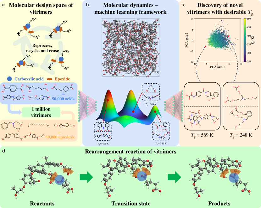
Figure 1: Schematic overview of this work. (a) A transesterification vitrimer comprises a carboxylic acid and an epoxide. The reversible covalent bond between acid and epoxide allows them to detach from and attach to each other, thus healing the polymer. The design space for vitrimers is defined as all possible combinations of 50,000 carboxylic acids and 50,000 epoxides and a vitrimer dataset is built by sampling from the design space. (b) We use calibrated MD simulations to calculate $T_{\mathrm{g}}$ on a subset of vitrimers. The vitrimer dataset and $T_{\mathrm{g}}$ are inputs to the VAE model. (c) By optimizing latent vectors according to desirable $T_{\mathrm{g}}$, novel vitrimers with $T_{\mathrm{g}}$ = 569 K and 248 K are discovered. (d) Schematic of rearrangement reaction in transesterification vitrimers where the carboxylic acid switches from one epoxide molecule to the other.

Advances in machine learning (ML) algorithms offer an opportunity to accelerate polymer discovery by learning from available data, revealing hidden patterns in material properties [13] and reducing the need for costly experiments and simulations [14]. Various ML methods have been employed to design organic molecules and polymers, including forward predictive models [15, 16, 17, 18], generative adversarial networks (GANs) [19, 20, 21], variational autoencoders (VAEs) [22, 23, 24, 25] and diffusion models [26, 27]. The trained ML models can be further used for high-throughput screening or conditioned upon physical properties to achieve the inverse design of polymers from properties of interest, such as glass transition temperature ($T_{\mathrm{g}}$)[16, 17], thermal conductivity[28, 29, 18], bandgap[25] and gas-separation properties [30, 18]. The success in these ML models depends on the choice of suitable representations, which is challenging due to the discrete and undefined degrees of freedom of molecules and polymers. To date, researchers have employed strings [31, 32], molecular fingerprints [33] and graphs [34] to represent and input molecules/monomers to ML models. In this work, we propose a graph VAE model employing dual graph encoders and overlapping latent dimensions [35, 36] which enable representation of multi-component vitrimers and controlled design of selective components simultaneously.

Last few years have seen an increased contribution to structures and properties databases of polymers and molecules such as ZINC15[37], ChemSpider[38] and PubChem[39]. However, a dataset of vitrimers to train such a deep generative model is lacking. Furthermore, part of the dataset needs to be associated with the property of interest ($T_{\mathrm{g}}$) to enable property-guided inverse design. To this end, we build the first vitrimer dataset derived from the online database ZINC15[37] and calculate $T_{\mathrm{g}}$ by calibrated MD simulations on a subset of vitrimers (Figure 1ab).

Leveraging this vitrimer dataset, we build an integrated MD-ML framework for discovery of bifunctional transesterification vitrimers with desirable properties specifically targeted $T_{\mathrm{g}}$ for the scope of this work (Figure 1b). Each vitrimer contains two reactive constituents (i.e., carboxylic acid and epoxide). Furthermore, the discrete nature of the molecules prohibits a smooth and continuous design space. For example, while molecules are interpretable to human, they are not interpretable to a numerical optimizer for design of vitrimers. To this end, we develop a VAE that receives as input a vitrimer represented by graphs and subgraphs of the constituents and produces a smooth and continuous latent space. In such a latent space, two similar vitrimers are located close to each other while an optimizer can traverse the space of all possible vitrimers. Our unique VAE framework offers both constituent-specific and joint latent spaces of the chemical constituents, i.e., continuous screening and optimization can be performed on just one or both of the constituents. This enables interpretability on the effects of optimizing over, e.g., acid only, epoxide only, or simultaneously acid and epoxide molecules. The efficacy of the framework is demonstrated by discovering novel vitrimers with $T_{\mathrm{g}}$ both within and well beyond the dataset. Specifically, while the $T_{\mathrm{g}}$ in the training data ranges from 250 K to 500 K, we discover vitrimers with $T_{\mathrm{g}}$ around 569 K and 248 K (Figure 1b). While we focus on transesterification vitrimers, the framework is sufficiently general to be applied to different types of vitrimers and their thermo-mechanical properties.

Results

Design space and data generation

We begin by creating a vitrimer dataset to train the VAE model. Since there are only a few available bifunctional transesterification vitrimers recorded in literature, we create a dataset of hypothetical vitrimers by combining carboxylic acids and epoxides. We first build two datasets by collecting available bifunctional carboxylic acids and epoxides from the online chemical compound database ZINC15 [37]. To further broaden the chemical space, we augment the datasets by adding hypothetical carboxylic acids and epoxides derived from available alcohols, olefins and phenols in the ZINC15 database. In both datasets, molecules satisfying all following rules are kept:

• Bifunctional constituents: carboxylic acid and epoxide-containing monomers have exactly two occurrences of their defining functional group (to restrict compositions to linear chains).

• Molecules with molecular weight smaller than 500 g/mol (to restrict the sizes of the molecular graphs and facilitate training of the graph VAE).

• Molecules with C, H, N, O elements only (to emulate the existing transesterification vitrimers).

After filtering, two datasets of around 322,000 carboxylic acids and 625,000 epoxides are constructed. To ensure synthesizability, we select the 50,000 acids and 50,000 epoxides with lowest synthetic accessibility (SA) scores [40] (i.e., those predicted to be easiest to synthesize). The final dataset is built by randomly sampling one million vitrimers from the design space of 2.5 billion possible combinations between the selected acids and epoxides, as shown in Figure 2a.

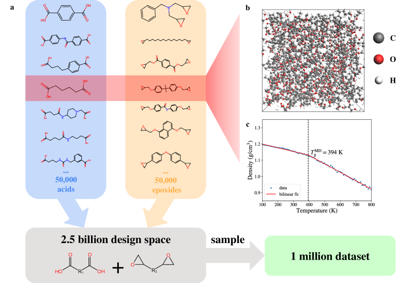
Figure 2: Schematic of the design space and data generation by MD simulations. (a) The vitrimer dataset is obtained by randomly sampling one million combinations between 50,000 bifunctional carboxylic acids and 50,000 epoxides derived from the ZINC15 database. (b) Snapshot of the annealed virtual specimen of the highlighted vitrimer (adipic acid and bisphenol A diglycidyl ether). (c) Density as a function of temperature obtained from MD simulations of the same vitrimer in (b). $T_{\mathrm{g}}$ is calculated as the intersection point of the bilinear fit.

To achieve property-guided inverse design, we further compute $T_{\mathrm{g}}$ of the vitrimers. Since MD simulations of the entire one-million dataset are computationally intractable, we calculate $T_{\mathrm{g}}$ of 8,424 vitrimers randomly sampled from the dataset. The quantity can cover a sufficient amount of vitrimers in the design space as well as keep the computational cost to a reasonable level. For each vitrimer, we create a virtual specimen then minimize and anneal the structure to remove local heterogeneities by slowly heating it to 800 K. A snapshot of the annealed system of an example vitrimer (adipic acid and bisphenol A diglycidyl ether) is shown in Figure 2b. The annealed structure is held at 800 K for an additional 50 ps and five specimens separated by 10 ps are obtained. To measure densities at different temperatures for $T_{\mathrm{g}}$ calculation, each specimen is cooled down from 800 K to 100 K linearly in steps of 10 K. By fitting a bilinear regression to the density-temperature profile, we calculate $T_{\mathrm{g}}$ as the intersection point of the two linear regressions (Figure 2c). Five replicate simulations are carried out from each specimen to reduce the noise due to the stochastic nature of MD. The distributions of average $T_{\mathrm{g}}$ and coefficient of variation (i.e., ratio of the standard deviation to the mean) in $T_{\mathrm{g}}$ of the vitrimers calculated by the five replicate MD simulations are shown in Supplementary Figures LABEL:tga and LABEL:tgb, respectively. The coefficients of variation in $T_{\mathrm{g}}$ of most of the vitrimers are below 0.1 with only a few around 0.15, indicating the low uncertainty in our MD simulations. Two vitrimer compositions with the corresponding density-temperature plots are presented in Supplementary Figures LABEL:tgc and LABEL:tgd, representing examples of vitrimers covering a wide range of $T_{\mathrm{g}}$. More details on MD simulations are provided in Supplementary Note LABEL:supp_md.

Due to the large difference in the cooling rate between MD simulations and experiments, MD-calculated $T_{\mathrm{g}}$ is typically overestimated compared with measurements from experiments. Compensating for this artifact, a previous work has achieved good correlation between MD-simulated $T_{\mathrm{g}}$ and experimental $T_{\mathrm{g}}$ on 315 polymers using ordinary least squares [41]. However, we find empirically that a simple two-parameter linear fit is insufficient to reduce the effect of larger noise in our MD simulations with smaller systems and fewer replicates. Instead, we employ a Gaussian process (GP) regression model to calibrate MD calculations against available experimental data. GP is a probabilistic model that uses a kernel (covariance) function to make probabilistic predictions based on the distance between the queried data point and a training set[42]. In order to construct a training dataset for the GP model, we gather 295 polymers from literature [43, 44], each with documented experimental $T_{\mathrm{g}}$. This data also includes available experimental data of three bifunctional transesterification vitrimers[11, 45, 46]. We calculate $T_{\mathrm{g}}$ for this experimental polymer dataset using the MD protocols described above and calculate the experiment-MD difference $\Delta T_{\mathrm{g}}$ for each of these polymers. To numerically represent both the polymers within the training set and the vitrimers to be calibrated as inputs for the GP model, we apply extended-connectivity fingerprints (ECFPs) [33] to the repeating units of the polymers, where asterisks (*) indicate connection points. We train the GP model to predict $\Delta T_{\mathrm{g}}$ from molecular fingerprints, as shown in Figure 3a. The calibrated $T_{\mathrm{g}}$ is defined as

$$T_{\mathrm{g}}=T_{\mathrm{g}}^{\mathrm{MD}}+\Delta T_{\mathrm{g}}^{\mathrm{GP}},$$ (1)

where $T_{\mathrm{g}}^{\mathrm{MD}}$ is the MD-calculated $T_{\mathrm{g}}$ and $\Delta T_{\mathrm{g}}^{\mathrm{GP}}$ is the experiment-MD $T_{\mathrm{g}}$ difference predicted by the GP model. More details on molecular fingerprints and the kernel function are provided in Supplementary Note LABEL:supp_gp.

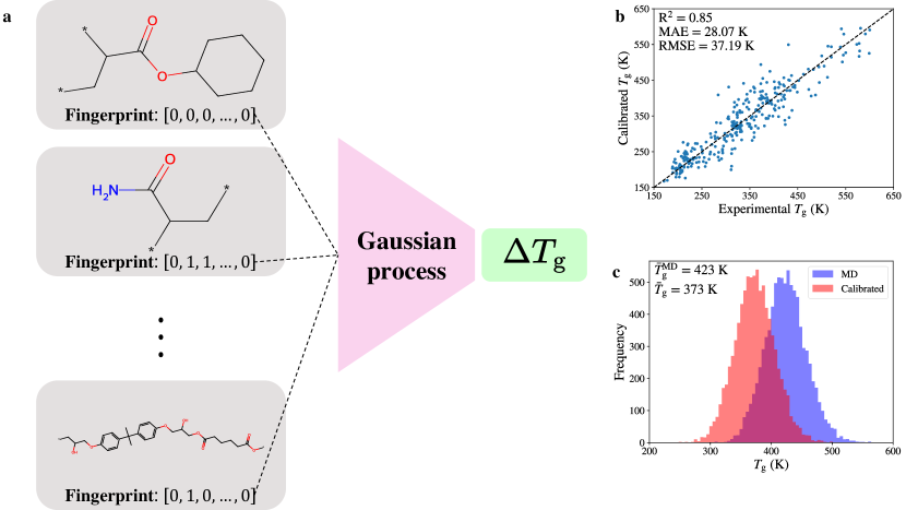
Figure 3: Calibration of the MD-calculated $T_{\mathrm{g}}$ by the GP regression model. (a) We train a GP model to predict the experiment-MD $T_{\mathrm{g}}$ difference from molecular fingerprints based on 295 polymers with recorded experimental $T_{\mathrm{g}}$ in literature. The trained GP model is applied to calibrate all vitrimers with MD-calculated $T_{\mathrm{g}}$ to predict their experimental $T_{\mathrm{g}}$. (b) Calibrated $T_{\mathrm{g}}$ vs. experimental $T_{\mathrm{g}}$ of all 295 polymers with leave-one-out cross validation. Each point is used as a test set which is not seen by the GP model. (c) The distributions of MD-calculated $T_{\mathrm{g}}$ before calibration and calibrated $T_{\mathrm{g}}$ by the GP model.

To evaluate the performance of our GP model, we implement leave-one-out cross validation (LOOCV). In this process, we train our GP model on all data points in the training set except one point and predict its calibrated $T_{\mathrm{g}}$. We repeat this process for all 295 polymers in the training set and compare the calibrated $T_{\mathrm{g}}$ with experimental $T_{\mathrm{g}}$ recorded in literature. An R² value of 0.85 between the calibrated $T_{\mathrm{g}}$ and experimental $T_{\mathrm{g}}$ is achieved (Figure 3b). For comparison, the results obtained by linear regression are presented in Supplementary Figure LABEL:othera. By utilizing the comprehensive GP model trained on the entire training dataset without LOOCV, we proceed to calibrate $T_{\mathrm{g}}$ of the vitrimer dataset calculated by MD simulations. The distributions of $T_{\mathrm{g}}$ of the vitrimers before and after GP calibration are shown in Figure 3c and both distributions approach Gaussian. The average $T_{\mathrm{g}}$ before and after calibration is 423 K and 373 K, respectively. Since the cooling rate in our MD simulations is 12 orders of magnitude higher than typical experiments, the difference of 50 K is consistent with the Williams–Landel–Ferry theory that estimates an increase in $T_{\mathrm{g}}$ of 3 to 5 K per order of magnitude increase in the cooling rate [47]. In this work, we denote $T_{\mathrm{g}}$ as the calibrated value from MD simulations, which serves as a proxy of the true experimental $T_{\mathrm{g}}$. It is also the input to the variational autoencoder and target of inverse design.

Variational autoencoder

The discrete nature of molecules makes it challenging for the generative model to learn a continuous latent space from discrete data of vitrimers. Any two molecules can have different degrees of freedom (e.g., number of atoms and bonds) and extra attention needs to be paid to the choice of representations. Here we adopt the hierarchical graph representation of molecules developed by a previous work [24]. A molecule is first represented as a graph $\mathcal{G}=(\mathcal{V},\mathcal{E})$ with atoms as nodes $\mathcal{V}$ and bonds as edges $\mathcal{E}$. We decompose the molecule $\mathcal{G}$ into $n$ motifs $\mathcal{M}_{1},...,\mathcal{M}_{n}$. Each motif $\mathcal{M}_{i}=(\mathcal{V}_{i},\mathcal{E}_{i})$ where $i\in\{1,...,n\}$ is a subgraph with atoms $\mathcal{V}_{i}$ and edges $\mathcal{E}_{i}$. The ensuing step involves a three-level hierarchical graph representation (see Supplementary Figure LABEL:hierarchical for a schematic illustration). The motif level $\mathcal{G}_{\mathcal{M}}$ establishes macroscopic connections in a tree-like structure, the attachment level $\mathcal{G}_{\mathcal{A}}$ encodes inter-motif connectivity via shared atoms, and the atom level $\mathcal{G}$ captures finer atomic relationships. More details about the hierarchical graph representation are presented in Supplementary Note LABEL:supp_repre.

We use a variational autoencoder (VAE) comprising two pairs of hierarchical encoders and decoders associated with the hierarchical representations of acid and epoxide molecules, respectively. A schematic of the framework is presented in Figure 4a. Each of the hierarchical encoder uses three message passing networks (MPNs) to encode the graphs from each of the three levels. The acid encoder $\mathcal{Q}^{\mathrm{a}}_{\phi^{\mathrm{a}}}$ (with trainable parameters $\phi^{\mathrm{a}}$) maps the molecular graph of the acid molecule $\mathcal{G}^{\mathrm{a}}$ into a pair of vectors $\boldsymbol{\mu}^{\mathrm{a}}\in\mathbb{R}^{d_{\mathrm{a}}}$ and $\log{\boldsymbol{\sigma}^{\mathrm{a}}}^{2}\in\mathbb{R}^{d_{\mathrm{a}}}$ of dimension $d_{\mathrm{a}}$, which are the mean and logarithm variance of a Gaussian distribution. Similarly, $\boldsymbol{\mu}^{\mathrm{e}}\in\mathbb{R}^{d_{\mathrm{e}}}$ and $\log{\boldsymbol{\sigma}^{\mathrm{e}}}^{2}\in\mathbb{R}^{d_{\mathrm{e}}}$ of dimension $d_{\mathrm{e}}$ are converted from the epoxide molecule $\mathcal{G}^{\mathrm{e}}$ by the epoxide encoder $\mathcal{Q}^{\mathrm{e}}_{\phi^{\mathrm{e}}}$.

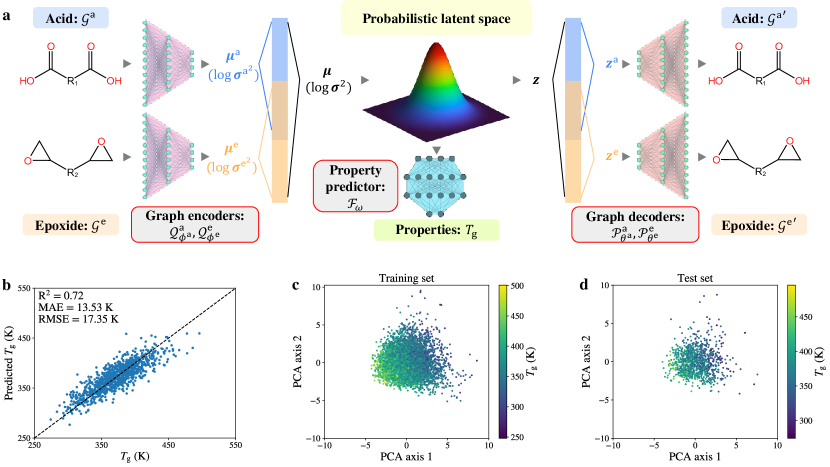
Figure 4: Illustration and performance of the VAE model. (a) The encoders convert acid and epoxide molecules into latent vectors $\boldsymbol{z}$ in a continuous latent space. The latent vectors $\boldsymbol{z}$ are further decoded into acid and epoxide molecules by the decoders. A property predictor is added to predict $T_{\mathrm{g}}$ from $\boldsymbol{z}$. The trainable components are highlighted by red borders. (b) Predicted $T_{\mathrm{g}}$ vs. true $T_{\mathrm{g}}$ of the test set. (c)(d) The distributions of latent vectors of labeled training set and test set visualized by principal component analysis (PCA).

We employ the attributed network embedding method [35, 36] to obtain the unified mean $\boldsymbol{\mu}$ and log variance $\log\boldsymbol{\sigma}^{2}$ of dimension $d$ embedding information of the acid and epoxide as well as their unified effects as follows. We define $d_{\mathrm{ae}}=d_{\mathrm{a}}+d_{\mathrm{e}}-d$ denoting the overlapping dimensions of $\boldsymbol{\mu}^{\mathrm{a}}$ and $\boldsymbol{\mu}^{\mathrm{e}}$ and calculate $\boldsymbol{\mu}$ by

$$\boldsymbol{\mu}=\underbrace{\begin{bmatrix}\mu_{1}^{\mathrm{a}}\\ \vdots\\ \mu_{d_{\mathrm{a}}-d_{\mathrm{ae}}}^{\mathrm{a}}\end{bmatrix}}_{\text{acid-specific}}\oplus\underbrace{\frac{1}{2}\left(\begin{bmatrix}\mu_{d_{\mathrm{a}}-d_{\mathrm{ae}}+1}^{\mathrm{a}}\\ \vdots\\ \mu_{d_{\mathrm{a}}}^{\mathrm{a}}\end{bmatrix}+\begin{bmatrix}\mu_{1}^{\mathrm{e}}\\ \vdots\\ \mu_{d_{\mathrm{ae}}}^{\mathrm{e}}\end{bmatrix}\right)}_{\text{shared}}\oplus\underbrace{\begin{bmatrix}\mu_{d_{\mathrm{ae}+1}}^{\mathrm{e}}\\ \vdots\\ \mu_{d_{\mathrm{e}}}^{\mathrm{e}}\end{bmatrix}}_{\text{epoxide-specific}},$$ (2)

where $\oplus$ denotes vector concatenation. The unified log variance vector $\log{\boldsymbol{\sigma}}^{2}$ is obtained similarly. Partially overlapping latent dimensions enables both independent and joint control as well as interpretability of embeddings of acid and epoxide. When exploring the latent space for new vitrimers later, it also allow us to change one part of the vitrimer but keep the other one unaltered.

The unified mean $\boldsymbol{\mu}$ and variance ${\boldsymbol{\sigma}}^{2}$ together describe a diagonal multivariate Gaussian distribution

$$\boldsymbol{z}\sim\mathcal{N}\left(\begin{bmatrix}\mu_{1},...,\mu_{d}\end{bmatrix}^{\intercal},\mathrm{diag}\left(\begin{bmatrix}\sigma_{1}^{2},...,\sigma_{d}^{2}\end{bmatrix}^{\intercal}\right)\right),$$ (3)

where $\boldsymbol{z}$ is the latent vector (representation) of dimension $d$ encoding necessary information of both input graphs $\mathcal{G}^{\mathrm{a}}$ and $\mathcal{G}^{\mathrm{e}}$. To keep differentiability and facilitate the training of VAE, the reparameterization trick [48] is used to sample the latent vector $\boldsymbol{z}$ from $\boldsymbol{\mu}$ and ${\boldsymbol{\sigma}}^{2}$ by

$$\boldsymbol{z}=\boldsymbol{\mu}+\boldsymbol{\epsilon}\odot\begin{bmatrix}\sigma_{1}^{2},...,\sigma_{d}^{2}\end{bmatrix}^{\intercal},$$ (4)

where $\boldsymbol{\epsilon}\sim\mathcal{N}(\boldsymbol{0},\boldsymbol{I})$ is a vector of dimension $d$ and $\odot$ denotes element-wise multiplication. The acid decoder $\mathcal{P}^{\mathrm{a}}_{\theta^{\mathrm{a}}}$ (with trainable parameters $\theta^{\mathrm{a}}$) is used to output the acid molecule ${\mathcal{G}^{\mathrm{a}}}^{\prime}$ from the acid-specific and shared dimensions of $\boldsymbol{z}$. Similarly, the epoxide decoder $\mathcal{P}^{\mathrm{e}}_{\theta^{\mathrm{e}}}$ is used to output the epoxide molecule ${\mathcal{G}^{\mathrm{e}}}^{\prime}$ from the epoxide-specific and shared dimensions of $\boldsymbol{z}$. More specifically, the decoders iteratively expand the graphs at three hierarchical levels. At step $t$, three multilayer perceptrons (MLPs) are used to predict the probability distributions of each motif node $\boldsymbol{p}_{\mathcal{M}_{t}}^{\prime}$, attachment node $\boldsymbol{p}_{\mathcal{A}_{t}}^{\prime}$ and atoms to be attached $\boldsymbol{p}_{(u,v)_{t}}^{\prime}$ (see Supplementary Note LABEL:supp_vae for more details). An additional MLP is used to predict the probability of backtracing $\boldsymbol{p}_{\mathrm{b}_{t}}^{\prime}$, i.e., when there will be no new neighbors to add to the motif node. Both decoders are optimized to accurately reconstruct the molecules, i.e., ${\mathcal{G}^{\mathrm{a}}}^{\prime}\approx\mathcal{G}^{\mathrm{a}}$ and ${\mathcal{G}^{\mathrm{e}}}^{\prime}\approx\mathcal{G}^{\mathrm{e}}$. Practically this is achieved by minimizing the error between all four predicted probability distributions with respect to the one-hot encoded ground truth, i.e., $\boldsymbol{p}_{\mathcal{M}_{t}}$, $\boldsymbol{p}_{\mathcal{A}_{t}}$, $\boldsymbol{p}_{(u,v)_{t}}$ and $\boldsymbol{p}_{\mathrm{b}_{t}}$ for $t=1,...,t_{\mathrm{max}}$ where $t_{\mathrm{max}}$ is the maximum number of iterations based on depth-first search of the input molecule (here for simplicity we omit superscripts a and e denoting acid and epoxide). Encoding input vitrimers as described here introduces an information bottleneck [49] within the latent representation. This bottleneck selectively retains necessary information required for accurate vitrimer reconstruction while largely reducing the dimensionality and complexity of original data. As a result, vitrimers with similar compositions occupy proximate positions in the latent space.

In order to achieve data-driven design and uncover novel vitrimers with the interested property, we establish a connection between the latent space and $T_{\mathrm{g}}$. This is accomplished by employing a neural network surrogate model that takes the latent vectors as inputs and outputs $T_{\mathrm{g}}$. Consequently, we modify the original VAE architecture and establish a projection from the latent space to $T_{\mathrm{g}}$ by incorporating the latent vectors $\boldsymbol{z}$ into a property prediction model $\mathcal{F}_{\omega}$ (with trainable parameters $\omega)$. Thereby, the predicted property is

$$T_{\mathrm{g}}^{\prime}=\mathcal{F}_{\omega}(\boldsymbol{z}).$$ (5)

We divide the training set into two datasets, one with $N$ vitrimers lacking property labels $\mathcal{D}=\{({\mathcal{G}^{\mathrm{a}}}^{(i)},{\mathcal{G}^{\mathrm{e}}}^{(i)}):i=1,...,N\}$, and one with $N_{\mathrm{prop}}$ vitrimer and $T_{\mathrm{g}}$ pairs $\mathcal{D}_{\mathrm{prop}}=\{({\mathcal{G}^{\mathrm{a}}}^{(i)},{\mathcal{G}^{\mathrm{e}}}^{(i)},T_{\mathrm{g}}^{(i)}):i=1,...,N_{\mathrm{prop}}\}$. Due to the large difference between $N$ and $N_{\mathrm{prop}}$ (999,000 vs. 7,424), we first train the VAE on an unsupervised basis with $\mathcal{D}$ and the property predictor is not optimized. Specifically,

$$\theta^{\mathrm{a}},\theta^{\mathrm{e}},\phi^{\mathrm{a}},\phi^{\mathrm{e}}\leftarrow\operatorname*{arg\,min}_{\theta^{\mathrm{a}},\theta^{\mathrm{e}},\phi^{\mathrm{a}},\phi^{\mathrm{e}}} \underbrace{\sum_{i=1}^{N}\left(\mathrm{CE}\left({\boldsymbol{p}_{\mathcal{M}}^{(i)}}^{\prime},\boldsymbol{p}_{\mathcal{M}}^{(i)}\right)+\mathrm{CE}\left({\boldsymbol{p}_{\mathcal{A}}^{(i)}}^{\prime},\boldsymbol{p}_{\mathcal{A}}^{(i)}\right)+\mathrm{CE}\left({\boldsymbol{p}_{(u,v)}^{(i)}}^{\prime},\boldsymbol{p}_{(u,v)}^{(i)}\right)+\mathrm{BCE}\left({\boldsymbol{p}_{\mathrm{b}}^{(i)}}^{\prime},\boldsymbol{p}_{\mathrm{b}}^{(i)}\right)\right)}_{\text{reconstruction loss}}$$

$$+ \underbrace{\lambda_{\mathrm{KL}}\frac{1}{N}\sum_{i=1}^{N}D_{\mathrm{KL}}\left(\mathcal{N}\left(\begin{bmatrix}\mu_{1}^{(i)},...,\mu_{d}^{(i)}\end{bmatrix}^{\intercal},\mathrm{diag}\left(\begin{bmatrix}{\sigma_{1}^{(i)}}^{2},...,{\sigma_{d}^{(i)}}^{2}\end{bmatrix}^{\intercal}\right)\right)\|\leavevmode\nobreak\ \mathcal{N}\left(\boldsymbol{0},\boldsymbol{I}\right)\right)}_{\text{Kullback\textendash Leibler divergence}},$$ (6)

where CE and BCE denote cross entropy loss and binary cross entropy loss [50], respectively. For simplicity, the subscript $t$ and superscripts a and e are omitted and all terms in reconstruction loss represent the sum over all decoding steps and over acid and epoxide. $\lambda_{\mathrm{KL}}>0$ is the regularization weight for Kullback–Leibler divergence. Training the VAE with $\mathcal{D}$ aims to construct well-trained encoders and decoders capable of accommodating a diverse array of vitrimers. The reconstruction loss ensures the accurate reconstruction of the encoded vitrimers with respect to both acid and epoxide molecules by the VAE. The Kullback–Leibler divergence (KLD)[51] is a statistical measure to quantify how different two distributions are from each other. Hence, by employing it as a loss term[48], we minimize the difference between the probability distribution of the latent space created by the encoder and the standard Gaussian distribution $\mathcal{N}(\boldsymbol{0},\boldsymbol{I})$. This helps in constructing a seamless and continuous latent space from which new samples can be generated using standard Gaussian distribution and allows us to discover and design novel vitrimers not present in the training set. The KLD is calculated as

$$D_{\mathrm{KL}}\left(\mathcal{N}\left(\begin{bmatrix}\mu_{1},...,\mu_{d}\end{bmatrix}^{\intercal},\mathrm{diag}\left(\begin{bmatrix}\sigma_{1}^{2},...,\sigma_{d}^{2}\end{bmatrix}^{\intercal}\right)\right)\|\leavevmode\nobreak\ \mathcal{N}\left(\boldsymbol{0},\boldsymbol{I}\right)\right)=\frac{1}{2}\sum_{j=1}^{d}[\mu_{j}^{2}+\sigma_{j}^{2}-\log(\sigma_{j}^{2})-1].$$ (7)

Subsequently, we use $\mathcal{D}_{\mathrm{prop}}$ to jointly train encoder, decoder and property predictor at the same time, i.e.,

$$\theta^{\mathrm{a}},\theta^{\mathrm{e}},\phi^{\mathrm{a}},\phi^{\mathrm{e}},{\color[rgb]{1,0,0}\omega}\leftarrow\operatorname*{arg\,min}_{\theta^{\mathrm{a}},\theta^{\mathrm{e}},\phi^{\mathrm{a}},\phi^{\mathrm{e}},{\color[rgb]{1,0,0}\omega}} \underbrace{\sum_{i=1}^{N_{\mathrm{prop}}}\left(\mathrm{CE}\left({\boldsymbol{p}_{\mathcal{M}}^{(i)}}^{\prime},\boldsymbol{p}_{\mathcal{M}}^{(i)}\right)+\mathrm{CE}\left({\boldsymbol{p}_{\mathcal{A}}^{(i)}}^{\prime},\boldsymbol{p}_{\mathcal{A}}^{(i)}\right)+\mathrm{CE}\left({\boldsymbol{p}_{(u,v)}^{(i)}}^{\prime},\boldsymbol{p}_{(u,v)}^{(i)}\right)+\mathrm{BCE}\left({\boldsymbol{p}_{\mathrm{b}}^{(i)}}^{\prime},\boldsymbol{p}_{\mathrm{b}}^{(i)}\right)\right)}_{\text{reconstruction loss}}$$

$$+ \underbrace{\lambda_{\mathrm{KL}}\frac{1}{N_{\mathrm{prop}}}\sum_{i=1}^{N_{\mathrm{prop}}}D_{\mathrm{KL}}\left(\mathcal{N}\left(\begin{bmatrix}\mu_{1}^{(i)},...,\mu_{d}^{(i)}\end{bmatrix}^{\intercal},\mathrm{diag}\left(\begin{bmatrix}{\sigma_{1}^{(i)}}^{2},...,{\sigma_{d}^{(i)}}^{2}\end{bmatrix}^{\intercal}\right)\right)\|\leavevmode\nobreak\ \mathcal{N}\left(\boldsymbol{0},\boldsymbol{I}\right)\right)}_{\text{Kullback\textendash Leibler divergence}}$$

$$+ \color[rgb]{1,0,0}\underbrace{\color[rgb]{0,0,0}\frac{1}{N_{\mathrm{prop}}}\sum_{i=1}^{N_{\mathrm{prop}}}\left({T_{\mathrm{g}}^{(i)}}^{\prime}-T_{\mathrm{g}}^{(i)}\right)^{2}}_{\text{property prediction loss}}.$$ (8)

The additional property prediction loss ensures accurate prediction of $T_{\mathrm{g}}$ from latent vectors. This joint training process reorganizes the latent space and places vitrimers with similar $T_{\mathrm{g}}$ in close proximity to each other. More details about hierarchical encoder and decoder, network architecture, training protocols and hyperparameters are presented in Supplementary Notes LABEL:supp_repre and LABEL:supp_vae.

Performance of the VAE

We first evaluate the ability of the VAE to reconstruct a given vitrimer. We encode the vitrimers in the test set into mean vectors of latent distribution $\boldsymbol{\mu}$ then decode $\boldsymbol{\mu}$ back to vitrimers. The ratio of successfully reconstructed (i.e., both carboxylic acid and epoxide decoded from $\boldsymbol{\mu}$ are identical to input molecules) is 85.4%, which demonstrates well-trained encoders and decoders capable of accommodating and reconstructing various vitrimers. Examples of ten vitrimers from the test set and the corresponding reconstructions are presented in Supplementary Figure LABEL:reconstruct. Eight vitrimers are perfectly reconstructed, while one component of vitrimers is decoded into different but similar molecules in the two unsuccessful examples.

We then assess the performance of the VAE to generate vitrimers. We sample 1,000 latent vectors $\boldsymbol{z}$ from standard Gaussian distribution and decode them into the carboxylic acid and epoxide molecules constituting vitrimers. 85.2% of the sampled vitrimers are valid, i.e., the composing acid and epoxide molecules are chemically valid and contain exactly two carboxylic acid and epoxide groups. Even though the decoders are not explicitly coded to only output carboxylic acids and epoxides (e.g., by making the decoders build up molecules based on two carboxylic acid and epoxide groups), most of the randomly sampled latent vectors are decoded to molecules containing the desired functionality. Examples of sampled vitrimers are shown in Supplementary Figure LABEL:sample. Components of the three invalid sampled vitrimers are also carboxylic acids and epoxides but do not have exactly two functional groups.

Apart from validity, we are also interested in the novelty and uniqueness of the generated vitrimers, which are defined as the ratio of sampled vitrimers which are not present in the training set and the expected fraction of unique vitrimers per sampled vitrimers, respectively. Results show that all of the 1,000 vitrimers sampled from the latent space are novel and unique, which greatly benefits the discovery of vitrimers by exploring the latent space.

We further examine the effect of joint training with the small dataset $\mathcal{D}_{\mathrm{prop}}$ containing a limited number of labeled vitrimers. All four metrics of the model before and after joint training are presented in Supplementary Table LABEL:metrics. The improved reconstruction accuracy and sample validity show that the second-step joint training enhances the performance of the model and that the encoders and decoders are not biased to the limited data in $\mathcal{D}_{\mathrm{prop}}$.

The property predictor maps latent space encoded from vitrimers to $T_{\mathrm{g}}$ and serves as a surrogate model for estimating $T_{\mathrm{g}}$ without the need for costly MD simulations. We evaluate the predictive power of the property predictor network by encoding the vitrimers in the test set into mean vectors $\boldsymbol{\mu}$ and predicting the associated $T_{\mathrm{g}}$. The predicted $T_{\mathrm{g}}$ and true $T_{\mathrm{g}}$ are compared in Figure 4b. A mean absolute error of 13.53 K indicates accurate prediction of $T_{\mathrm{g}}$ by the property predictor which facilitates the inverse design process.

The VAE jointly trained with the property predictor organizes the latent space such that vitrimers exhibiting similar properties are positioned in the vicinity of each other. We examine the distribution of latent vectors and corresponding $T_{\mathrm{g}}$ of the labeled datasets using principal component analysis (PCA). As shown in Figures 4c and 4d, the distribution of all latent vectors shows an obvious gradient in both training and test sets, where vitrimers with higher $T_{\mathrm{g}}$ cluster in the lower left region. Such a well-structured latent space based on properties benefits the inverse design process. For comparison, the latent space before joint training is presented in Supplementary Figure LABEL:unjoint. The much less obvious trend confirms the effect of joint training on latent space organization.

Interpretable exploration of the latent space

The well trained, continuous latent space enables us to discover new vitrimers by exploring the latent space through modifications of latent vectors $\boldsymbol{z}$. For example, we start with the latent vector $\boldsymbol{z}_{0}$ of a known vitrimer (adipic acid and bisphenol A diglycidyl ether) as origin and sample latent vectors in the neighborhood by perturbing $\boldsymbol{z}_{0}$. Previous works that employ multi-component VAEs (i.e., VAEs with multiple encoders and decoders) simply add embedding or mean (log variance) vectors from encoders to derive the unified latent vector $\boldsymbol{z}$ [30]. The effect of different components is not considered individually and a change in $\boldsymbol{z}$ leads to potential changes in all components. The partially overlapping latent dimensions (Equation 2) allow us to explore the vicinity of the origin $\boldsymbol{z}_{0}$ along different axes by adding noise to acid-specific latent dimensions (first $d_{\mathrm{a}}$ dimensions of $\boldsymbol{z}_{0}$), epoxide-specific latent dimensions (last $d_{\mathrm{e}}$ dimensions of $\boldsymbol{z}_{0}$) and all latent dimensions of $\boldsymbol{z}_{0}$ (details are provided in Supplementary Note LABEL:supp_explore). Consequently, novel vitrimers with changes in only acid, only epoxide and both components are identified by decoding the latent vectors modified along three axes, as shown in Figures 5a-c. The decoded vitrimers present variety in molecular structures without significant changes in $T_{\mathrm{g}}$ (Figure 5f) due to limited search region in latent space, which opens an opportunity to tailor a specific vitrimer to its novel variants with different molecular structures but preserve certain property similarity.

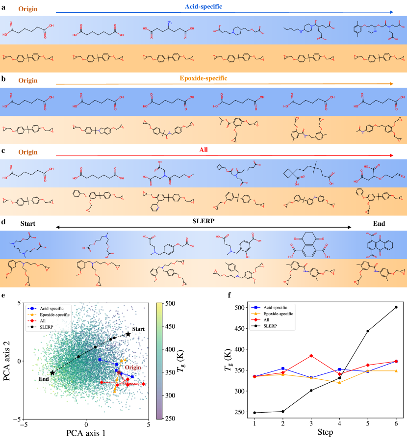
Figure 5: Exploration in the latent space to discover novel vitrimers. (a)(b)(c) Starting with a known vitrimer as origin (adipic acid and bisphenol A diglycidyl ether), vitrimers are discovered by perturbing its latent vector in (a) acid-specific dimensions, (b) epoxide-specific dimensions and (c) all dimensions. (d) Novel vitrimers identified along the interpolation path between two vitrimers in the training set. (e) The distribution of discovered vitrimers is visualized in the latent space by PCA. (f) $T_{\mathrm{g}}$ of discovered vitrimers by the four methods as functions of steps which indicate the increasing distances from the origin (start) vitrimer (step 1). All presented $T_{\mathrm{g}}$ values of are validated by MD simulations and GP calibration.

Besides neighborhood search, we perform an interpolation between two points in the latent space and identify a series of new vitrimers along the path. Figure 5d presents an example of spherical interpolation (SLERP) [52] between vitrimers with highest and lowest $T_{\mathrm{g}}$ in the training set. As opposed to linear interpolation (LERP), we use SLERP because Gaussian distribution in high dimensions closely follows the surface of a hypersphere. The decoded vitrimers show a smooth transition from the low-$T_{\mathrm{g}}$ vitrimer with linear structure to the high-$T_{\mathrm{g}}$ vitrimer with more aromatic nature. The continuous transition between molecular structures and $T_{\mathrm{g}}$ (Figure 5f) evidences the smoothness of the latent space with associated $T_{\mathrm{g}}$. More details on spherical and linear interpolation schemes are presented in Supplementary Note LABEL:supp_explore.

Inverse design by Bayesian optimization

The VAE together with the property predictor succeeds in learning the hidden relationships between latent space and $T_{\mathrm{g}}$ of vitrimers, which allows us to tailor vitrimer compositions to desirable $T_{\mathrm{g}}$ even beyond the training regime. Although we have achieved forward projection from the vitrimer space (or latent space) to property space, the inverse mapping is more challenging due to the fact that multiple distinct vitrimers could have a similar $T_{\mathrm{g}}$. To achieve inverse design of vitrimers with optimal or desirable $T_{\mathrm{g}}$, we employ batch Bayesian optimization to identify the latent vectors $\boldsymbol{z}$ that have the potential to be decoded into vitrimers with target $T_{\mathrm{g}}$. The proposed candidates are further validated by MD simulations with GP calibration, and the optimal solutions with desirable true $T_{\mathrm{g}}$ are found. Due to the discrete nature of molecules, the latent vectors proposed by the optimization process may lead to invalid molecules. Furthermore, since the discrete molecules are projected onto a continuous latent space by the VAE, it is inevitable that multiple distinct latent vectors in the neighborhood can be decoded into the same vitrimer but are associated with different $T_{\mathrm{g}}$ predicted by the property predictor. This severely limits the accuracy and efficiency of the optimization process. To this end, we add an additional decoding-encoding step before passing $\boldsymbol{z}$ to the property predictor to predict $T_{\mathrm{g}}$ (see Supplementary Figure LABEL:boflowa). More specifically, when evaluating the $T_{\mathrm{g}}$ of a point of interest $\boldsymbol{z}$ in the latent space during the optimization process, $\boldsymbol{z}$ is first decoded into a carboxylic acid and an epoxide. If both molecules are valid, they are passed to the encoders to obtain the reconstructed mean vector $\boldsymbol{\mu}_{\mathrm{recon}}$, which is further passed to the property predictor to evaluate the $T_{\mathrm{g}}$. In this way, the Bayesian optimization algorithm is able to search for the potential candidates with desirable $T_{\mathrm{g}}$ efficiently without proposing the same vitrimer for a large number of iterations. More details about Bayesian optimization are provided in Supplementary Note LABEL:supp_bo.

To demonstrate the effectiveness of our inverse design framework, we use Bayesian optimization to discover novel vitrimers with three different objectives: maximum $T_{\mathrm{g}}$, $T_{\mathrm{g}}=373\leavevmode\nobreak\ \mathrm{K}$ and $T_{\mathrm{g}}=248\leavevmode\nobreak\ \mathrm{K}$. For each target, four examples of discovered vitrimers are presented in Figure 6. For the first target (maximum $T_{\mathrm{g}}$), our VAE model generates novel vitrimers with MD-validated $T_{\mathrm{g}}$ beyond the upper bound of $T_{\mathrm{g}}$ in the training data (500 K) and thereby expands the limits in thermal properties of bifunctional transesterification vitrimers. The Bayesian optimization procedures are able to probe the latent space outside of the training domain and propose novel vitrimers with extreme properties, which is difficult for traditional forward modeling methods to find. For the second target, the Bayesian optimization algorithm effectively searches the latent space and successfully proposes vitrimers with the exact target $T_{\mathrm{g}}$ of 373 K. The corresponding latent vectors are spread out in the latent space and the vitrimer compositions present significant molecular variety. For the third target which is the lower bound of the training domain (248 K), the proposed vitrimers (especially carboxylic acids) are more similar to each other and occupy a small region in the latent space. This can be attributed to the fact that there are not many linear molecules with more aliphatic nature in the 50,000 acids or epoxides making the training set. As a result, the distribution of these vitrimers with low $T_{\mathrm{g}}$ is insufficiently captured by the VAE and the proposed candidates of low-$T_{\mathrm{g}}$ vitrimers are restrained by the limited training data.

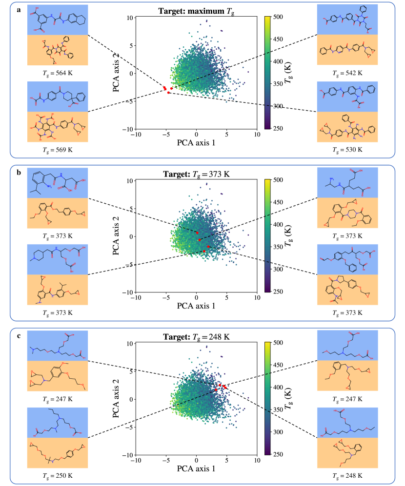
Figure 6: Novel vitrimers with different target $T_{\mathrm{g}}$ by inverse design based on Bayesian optimization and their locations in the latent space visualized by PCA. (a) Maximum $T_{\mathrm{g}}$. (b) Target $T_{\mathrm{g}}=373\leavevmode\nobreak\ \mathrm{K}$. (c) Target $T_{\mathrm{g}}=248\leavevmode\nobreak\ \mathrm{K}$. All presented $T_{\mathrm{g}}$ values of proposed vitrimers are validated by MD simulations and GP calibration.

More examples of novel vitrimers discovered by Bayesian optimization and their synthetic accessibility (SA) scores are presented in Supplementary Figure LABEL:morebo. For the first target, all ten proposed vitrimers have validated $T_{\mathrm{g}}$ larger than 500 K, which indicates the effective extrapolation beyond the training domain by our framework. For the other two targets of finding vitrimers with exact target $T_{\mathrm{g}}$, the discovered vitrimers present $T_{\mathrm{g}}$ within a range of 2 K around the target and maintain considerable molecular diversity, proving the high accuracy in the inverse design process. We compare $T_{\mathrm{g}}$ of the designed vitrimers with nine commonly used polymers in Supplementary Figure LABEL:tgbarchart. Our proposed vitrimers cover a wide range of $T_{\mathrm{g}}$ suitable for various applications from coating materials to aerospace polymers. With further tuning of the target, our framework has the potential to discover vitrimer compositions with any $T_{\mathrm{g}}$ within an expanded range and expedite the widespread applications of sustainable polymers in various industries.

We carry out further analysis based on the molecular descriptors of ten proposed vitrimers for each target. The molecular descriptors except density are calculated from the vitrimer repeating units (Supplementary Figure LABEL:crosslink with $n=1$) by the Modred package [53]. Density of each vitrimer at 300 K is calculated by MD simulations. The relevant descriptors of designed low, medium and high temperature vitrimers are presented in Supplementary Figure LABEL:descriptor. The vitrimers with higher $T_{\mathrm{g}}$ have larger average molecular weight, higher density, more heavy atoms and multiple bonds and fewer rotatable bonds. Consequently, the chains in these vitrimers are more rigid and less mobile, which agrees with the common knowledge of structure-$T_{\mathrm{g}}$ relationships in polymers.

Discussion

We develop an integrated MD-ML framework for inverse design of bifunctional transesterification vitrimers with desirable $T_{\mathrm{g}}$. A diverse vitrimer dataset is built for the first time from the ZINC15 database [37]. High-throughput MD simulations with a GP calibration model are employed to calculate $T_{\mathrm{g}}$ on a subset of vitrimers. The dataset is used to train a VAE model with dual graph encoders and decoders which enables representation and design of the desired vitrimer components. This further provides flexibility in exploring the latent space along different axes for novel vitrimers. We demonstrate the high accuracy and efficiency of our framework in discovering novel vitrimers with three different targets of $T_{\mathrm{g}}$ even beyond the training distribution. The proposed vitrimers achieve both molecular variety and desirable $T_{\mathrm{g}}$ within 2 K range around the target, which make them ideal candidates for sustainable polymers for different applications. With slight modifications on the VAE architecture, the proposed framework can be extended to a wide range of properties (for example, Young’s modulus, thermal conductivity, and topology freezing temperature) and other types of polymers. The complete workflow of design and validation opens an opportunity for high-fidelity inverse design of multi-component polymeric materials.

Methods

Details of MD simulations (Section LABEL:supp_md), GP calibration model (Section LABEL:supp_gp), hierarchical representation of molecules (Section LABEL:supp_repre), VAE architecture and training protocols (Section LABEL:supp_vae), VAE performance (Section LABEL:supp_performance), exploration of the latent space (Section LABEL:supp_explore), Bayesian optimization (Section LABEL:supp_bo) and analysis of proposed vitrimers (Section LABEL:supp_analysis) are provided in Supplementary Information.

Data and code availability

All generated vitrimer data (molecules in SMILES, density-temperature profiles and calculated $T_{\mathrm{g}}$), code and data used for the GP calibration model and code used for the VAE framework and Bayesian optimization will be made openly available at the time of publication.

Authors contributions

Y.Z.: Methodology, Software, Validation, Data Curation, Visualization, Writing, Reviewing and Editing; P.T.: Methodology, Software, Reviewing and Editing; J.A.S: Methodology, Software, Reviewing and Editing; Z.L.: Software, Reviewing and Editing; S.Z.: Reviewing and Editing; B.H.N.: Reviewing and Editing, Supervision; S.K.: Conceptualization, Methodology, Reviewing and Editing, Supervision; A.V.: Conceptualization, Methodology, Reviewing and Editing, Supervision.

Competing interests

J.A.S., Z.L., S.Z. and B.H.N. are employees of Microsoft Corporation. Y.Z., P.T., S.K. and A.V. declare no competing interests.

References

- [1] Young, R. J. & Lovell, P. A. Introduction to polymers (CRC press, 2011).
- [2] Krishnakumar, B. et al. Vitrimers: Associative dynamic covalent adaptive networks in thermoset polymers. \JournalTitleChemical Engineering Journal 385, 123820 (2020).
- [3] Montarnal, D., Capelot, M., Tournilhac, F. & Leibler, L. Silica-like malleable materials from permanent organic networks. \JournalTitleScience 334, 965–968 (2011).
- [4] Jin, Y., Lei, Z., Taynton, P., Huang, S. & Zhang, W. Malleable and recyclable thermosets: the next generation of plastics. \JournalTitleMatter 1, 1456–1493 (2019).
- [5] Valavala, P. & Odegard, G. Modeling techniques for determination of mechanical properties of polymer nanocomposites. \JournalTitleReviews on Advanced Materials Science 9, 34–44 (2005).
- [6] Vashisth, A., Ashraf, C., Bakis, C. E. & van Duin, A. C. Effect of chemical structure on thermo-mechanical properties of epoxy polymers: Comparison of accelerated reaxff simulations and experiments. \JournalTitlePolymer 158, 354–363 (2018).
- [7] Hoogenboom, R., Meier, M. A. & Schubert, U. S. Combinatorial methods, automated synthesis and high-throughput screening in polymer research: past and present. \JournalTitleMacromolecular rapid communications 24, 15–32 (2003).
- [8] Hansson, T., Oostenbrink, C. & van Gunsteren, W. Molecular dynamics simulations. \JournalTitleCurrent opinion in structural biology 12, 190–196 (2002).
- [9] Vashisth, A., Ashraf, C., Zhang, W., Bakis, C. E. & Van Duin, A. C. Accelerated reaxff simulations for describing the reactive cross-linking of polymers. \JournalTitleThe Journal of Physical Chemistry A 122, 6633–6642 (2018).
- [10] Yu, K.-q., Li, Z.-s. & Sun, J. Polymer structures and glass transition: A molecular dynamics simulation study. \JournalTitleMacromolecular theory and simulations 10, 624–633 (2001).
- [11] Kamble, M. et al. Reversing fatigue in carbon-fiber reinforced vitrimer composites. \JournalTitleCarbon 187, 108–114 (2022).
- [12] Kranenburg, J. M., Tweedie, C. A., van Vliet, K. J. & Schubert, U. S. Challenges and progress in high-throughput screening of polymer mechanical properties by indentation. \JournalTitleAdvanced Materials 21, 3551–3561 (2009).
- [13] Guo, K., Yang, Z., Yu, C.-H. & Buehler, M. J. Artificial intelligence and machine learning in design of mechanical materials. \JournalTitleMaterials Horizons 8, 1153–1172 (2021).
- [14] Barnett, J. W. et al. Designing exceptional gas-separation polymer membranes using machine learning. \JournalTitleScience advances 6, eaaz4301 (2020).
- [15] Jørgensen, P. B. et al. Machine learning-based screening of complex molecules for polymer solar cells. \JournalTitleThe Journal of chemical physics 148 (2018).
- [16] Tao, L., Chen, G. & Li, Y. Machine learning discovery of high-temperature polymers. \JournalTitlePatterns 2 (2021).
- [17] Tao, L., Varshney, V. & Li, Y. Benchmarking machine learning models for polymer informatics: an example of glass transition temperature. \JournalTitleJournal of Chemical Information and Modeling 61, 5395–5413 (2021).
- [18] Yang, J., Tao, L., He, J., McCutcheon, J. R. & Li, Y. Machine learning enables interpretable discovery of innovative polymers for gas separation membranes. \JournalTitleScience Advances 8, eabn9545 (2022).
- [19] Kadurin, A., Nikolenko, S., Khrabrov, K., Aliper, A. & Zhavoronkov, A. drugan: an advanced generative adversarial autoencoder model for de novo generation of new molecules with desired molecular properties in silico. \JournalTitleMolecular pharmaceutics 14, 3098–3104 (2017).
- [20] Sanchez-Lengeling, B., Outeiral, C., Guimaraes, G. L. & Aspuru-Guzik, A. Optimizing distributions over molecular space. an objective-reinforced generative adversarial network for inverse-design chemistry (organic). \JournalTitleChemRxiv (2017).
- [21] Prykhodko, O. et al. A de novo molecular generation method using latent vector based generative adversarial network. \JournalTitleJournal of Cheminformatics 11, 1–13 (2019).
- [22] Gómez-Bombarelli, R. et al. Automatic chemical design using a data-driven continuous representation of molecules. \JournalTitleACS central science 4, 268–276 (2018).
- [23] Jin, W., Barzilay, R. & Jaakkola, T. Junction tree variational autoencoder for molecular graph generation. In International conference on machine learning, 2323–2332 (PMLR, 2018).
- [24] Jin, W., Barzilay, R. & Jaakkola, T. Hierarchical generation of molecular graphs using structural motifs. In International conference on machine learning, 4839–4848 (PMLR, 2020).
- [25] Batra, R. et al. Polymers for extreme conditions designed using syntax-directed variational autoencoders. \JournalTitleChemistry of Materials 32, 10489–10500 (2020).
- [26] Xu, M. et al. Geodiff: A geometric diffusion model for molecular conformation generation. \JournalTitlearXiv preprint arXiv:2203.02923 (2022).
- [27] Hoogeboom, E., Satorras, V. G., Vignac, C. & Welling, M. Equivariant diffusion for molecule generation in 3d. In International conference on machine learning, 8867–8887 (PMLR, 2022).
- [28] Wu, S. et al. Machine-learning-assisted discovery of polymers with high thermal conductivity using a molecular design algorithm. \JournalTitleNpj Computational Materials 5, 66 (2019).
- [29] Zhu, M.-X., Song, H.-G., Yu, Q.-C., Chen, J.-M. & Zhang, H.-Y. Machine-learning-driven discovery of polymers molecular structures with high thermal conductivity. \JournalTitleInternational Journal of Heat and Mass Transfer 162, 120381 (2020).
- [30] Yao, Z. et al. Inverse design of nanoporous crystalline reticular materials with deep generative models. \JournalTitleNature Machine Intelligence 3, 76–86 (2021).
- [31] Weininger, D. Smiles, a chemical language and information system. 1. introduction to methodology and encoding rules. \JournalTitleJournal of chemical information and computer sciences 28, 31–36 (1988).
- [32] Krenn, M., Häse, F., Nigam, A., Friederich, P. & Aspuru-Guzik, A. Self-referencing embedded strings (selfies): A 100% robust molecular string representation. \JournalTitleMachine Learning: Science and Technology 1, 045024 (2020).
- [33] Rogers, D. & Hahn, M. Extended-connectivity fingerprints. \JournalTitleJournal of chemical information and modeling 50, 742–754 (2010).
- [34] Kearnes, S., McCloskey, K., Berndl, M., Pande, V. & Riley, P. Molecular graph convolutions: moving beyond fingerprints. \JournalTitleJournal of computer-aided molecular design 30, 595–608 (2016).
- [35] Lerique, S., Abitbol, J. L. & Karsai, M. Joint embedding of structure and features via graph convolutional networks. \JournalTitleApplied Network Science 5, 1–24 (2020).
- [36] Zheng, L., Karapiperis, K., Kumar, S. & Kochmann, D. M. Unifying the design space and optimizing linear and nonlinear truss metamaterials by generative modeling. \JournalTitleNature Communications 14, 7563 (2023).
- [37] Sterling, T. & Irwin, J. J. Zinc 15–ligand discovery for everyone. \JournalTitleJournal of chemical information and modeling 55, 2324–2337 (2015).
- [38] Pence, H. E. & Williams, A. Chemspider: an online chemical information resource (2010).
- [39] Kim, S. et al. Pubchem 2023 update. \JournalTitleNucleic acids research 51, D1373–D1380 (2023).
- [40] Ertl, P. & Schuffenhauer, A. Estimation of synthetic accessibility score of drug-like molecules based on molecular complexity and fragment contributions. \JournalTitleJournal of cheminformatics 1, 1–11 (2009).
- [41] Afzal, M. A. F. et al. High-throughput molecular dynamics simulations and validation of thermophysical properties of polymers for various applications. \JournalTitleACS Applied Polymer Materials 3, 620–630 (2020).
- [42] Deringer, V. L. et al. Gaussian process regression for materials and molecules. \JournalTitleChemical Reviews 121, 10073–10141 (2021).
- [43] Bicerano, J. Prediction of polymer properties (cRc Press, 2002).
- [44] Chemical retrieval on the web (crow). http://www.polymerdatabase.com/.
- [45] Ran, Y., Zheng, L.-J. & Zeng, J.-B. Dynamic crosslinking: An efficient approach to fabricate epoxy vitrimer. \JournalTitleMaterials 14, 919 (2021).
- [46] Wu, J. et al. Natural glycyrrhizic acid: improving stress relaxation rate and glass transition temperature simultaneously in epoxy vitrimers. \JournalTitleGreen Chemistry 23, 5647–5655 (2021).
- [47] Ediger, M. D., Angell, C. A. & Nagel, S. R. Supercooled liquids and glasses. \JournalTitleThe journal of physical chemistry 100, 13200–13212 (1996).
- [48] Kingma, D. P. & Welling, M. Auto-encoding variational bayes. \JournalTitlearXiv preprint arXiv:1312.6114 (2013).
- [49] Tishby, N., Pereira, F. C. & Bialek, W. The information bottleneck method. \JournalTitlearXiv preprint physics/0004057 (2000).
- [50] Good, I. J. Rational decisions. \JournalTitleJournal of the Royal Statistical Society: Series B (Methodological) 14, 107–114 (1952).
- [51] Kullback, S. & Leibler, R. A. On information and sufficiency. \JournalTitleThe annals of mathematical statistics 22, 79–86 (1951).
- [52] Shoemake, K. Animating rotation with quaternion curves. In Proceedings of the 12th annual conference on Computer graphics and interactive techniques, 245–254 (1985).
- [53] Moriwaki, H., Tian, Y.-S., Kawashita, N. & Takagi, T. Mordred: a molecular descriptor calculator. \JournalTitleJournal of cheminformatics 10, 1–14 (2018).